Colorizing Monochromatic Radiance Fields

Abstract

Though Neural Radiance Fields (NeRF) can produce colorful 3D representations of the world by using a set of 2D images, such ability becomes non-existent when only monochromatic images are provided. Since color is necessary in representing the world, reproducing color from monochromatic radiance fields becomes crucial. To achieve this goal, instead of manipulating the monochromatic radiance fields directly, we consider it as a representation-prediction task in the Lab color space. By first constructing the luminance and density representation using monochromatic images, our prediction stage can recreate color representation on the basis of an image colorization module. We then reproduce a colorful implicit model through the representation of luminance, density, and color. Extensive experiments have been conducted to validate the effectiveness of our approaches. Our project page: https://liquidammonia.github.io/color-nerf.

Introduction

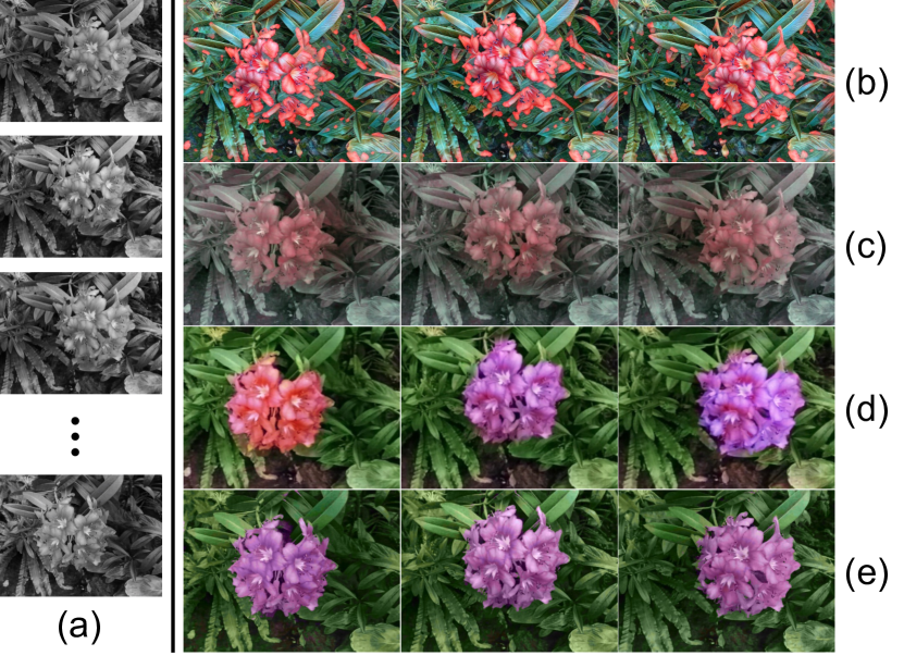
Figure 1: With multi-view monochromatic images (a) as inputs, (b-e) are three novel views synthesised by NeRF models. Existing color editing NeRFs (b) ARF (Zhang et al. 2022) and (c) CLIP-NeRF (Wang et al. 2022a) could not guarantee pixel-wise color adherence, while using “colorize-then-fuse” solution (d) CT² (Weng et al. 2022)+NeRF) suffers from color inconsistency across different views. The proposed ColorNeRF (e) can generate a more plausible and vivid colorized NeRF compared to previous models.

Neural Radiance Fields (NeRF) (Mildenhall et al. 2020) is able to create a colorful 3D representation of the world by using a set of 2D images. Can this created implicit 3D model still be colorful when only monochromatic images are available?

The answer is frustrating. The original design of NeRF is unable to create a colorful appearance from monochrome, and colorizing the monochromatic radiance fields using external forces seems to be the only option. Colorization is a classical problem being studied for more than a decade (Cheng, Yang, and Sheng 2015; Ironi, Cohen-Or, and Lischinski 2005; Levin, Lischinski, and Weiss 2004; Luan et al. 2007), with various applications in artistic creation, and legacy photo restoration. During its evolution on images/videos, there are two common standards that a good colorization scheme should follow: 1) plausibility, which requires the colorized results to demonstrate visually reasonable appearance (Iizuka, Simo-Serra, and Ishikawa 2016; Larsson, Maire, and Shakhnarovich 2016); 2) vividness, which ensures the high level of saturation for colorized results (Weng et al. 2022; Wu et al. 2021; Zhang, Isola, and Efros 2016; Zhang et al. 2017). These standards should be applied to colorizing monochromatic radiance fields as well, but how to achieve this remains an open problem.

Directly manipulating radiance fields seems to be a straightforward way to achieve this goal of colorization. One solution is to regard the color as a kind of “style” and then transfer the style into radiance fields (Zhang et al. 2022). However, as displayed in Fig. 1(b), since such a strategy cannot guarantee pixel-wise color adherence, the color can only distribute on radiance fields irregularly, thus violating the plausibility standard. A different approach involves manipulating the color attributes in radiance fields directly (Tojo and Umetani 2022; Wang et al. 2022a). This technique is intended for replacing colors by identifying the current color attributes and replacing them with new ones. However, it is not applicable to monochromatic radiance fields where there are no existing color attributes. As displayed in Fig. 1(c), the inability to perceive color palettes when using “direct manipulating” approaches (Wang et al. 2022a) on monochromatic radiance fields leaves rendered results below the vividness standard.

Another alternative is the “colorize-then-fuse” solution, i.e, first colorize monochromatic images and then fuse them for radiance field construction. However, without considering the view-dependent correlation, the examples colorized by image-based approaches cannot guarantee color consistency in the constructed radiance fields, as displayed in Fig. 1(d), which also obviously violates the plausibility standard. However, despite the unsatisfactory plausibility across views, this paradigm indeed achieves better vividness than directly manipulating radiance fields, compared with Fig. 1(b) and Fig. 1(c). This is partly because of the operation on complementing the missing color channels (Huang, Zhao, and Liao 2022; Zhang, Isola, and Efros 2016; Wu et al. 2021) in the CIE Lab color space as a channel-prediction task (Iizuka, Simo-Serra, and Ishikawa 2016; Weng et al. 2022; Zhang, Isola, and Efros 2016), i.e., inferring the missing a and b channels from the given L channel (monochromatic image). As opposed to producing three-channel RGB outputs, such an operation allows the neural network to focus only on the generation of two color channels (Anwar et al. 2020), which reduces computational costs and uncertainty during colorization.

Based on the above observations, in this paper, we propose ColorNeRF, to colorize monochromatic radiance fields by predicting the missing representation of color channels. As displayed in Fig. 2, ColorNeRF first builds luminance and density radiance fields by solely using monochromatic images and then infers the color representation for channel $a$ and $b$. Instead of building the radiance fields via directly altering in the image domain like the “colorize-then-fuse” paradigm, we inject color knowledge into the predicted representations from an off-the-shelf colorization module (Weng et al. 2022) based on a newly proposed query-based colorization strategy. By gradually imposing changes on the predicted representation, our model can finally maintain color consistency for better plausibility. A histogram-guided purification module and a classification-based color injection module are further proposed to better address color plausibility and enhance the vividness.

To sum up, ColorNeRF is the first approach that achieves rendering plausible and vivid radiance fields from monochromatic images via the following contributions:

• a representation prediction paradigm tailored to recreate colors for monochromatic radiance fields;

• a query-based colorization strategy and a histogram-guided purification module for maintaining strong plausibility, and

• a classification-based color injection module for achieving high vividness in colorized results.

Extensive experiments on LLFF dataset (Mildenhall et al. 2019) and our own captured scenes demonstrate that ColorNeRF achieves state-of-the-art results with better plausibility and vividness in quantitative and qualitative measurements. We also show the colorful NeRF generated from real monochromatic inputs, e.g., monochrome photography and classical movies.

Related work

Image colorization.

Several methods have been proposed to address the plausibility and vividness in colorization. Automatic colorization methods use a single monochromatic image as the input. It is a highly ill-posed task while requires estimating two missing color channels from one monochormatic channel. Early approaches rely on the local freature extraction (Guadarrama et al. 2017; Larsson, Maire, and Shakhnarovich 2016; Zhang, Isola, and Efros 2016). Later, better colorization can be achieved via the generative models (Cao et al. 2017; Vitoria, Raad, and Ballester 2020). Several other studies (Geonung et al. 2022; Wu et al. 2021; Zhao et al. 2020) have focused on utilizing external prior knowledge from other low-level vision tasks. Other works focus on how to inject multi-modal user-guided features to conduct conditional colorization. For example, stroke-based approaches (Yun et al. 2023; Zhang, Isola, and Efros 2016; Zhang et al. 2017) and text-based methods (Chang et al. 2022; Chen et al. 2018; Huang, Zhao, and Liao 2022) are proposed to adopt necessary attention features. In terms of image/video-based colorization, the above methods have pushed the boundaries for plausibility and vividness, but still cannot achieve these two goals for monochromatic radiance fields used to implicitly represent 3D space, which we hope to achieve in this paper.

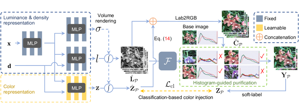
Figure 2: The overall pipeline of the proposed ColorNeRF. With rays from multiple viewpoints as inputs, luminance and density representation is first constructed with supervision over the ground truth monochromatic images, yielding monochromatic image patches $\hat{\mathbf{L}}_{\mathcal{P}}$. Then we predict color with an off-the-shelf 2D colorization module $\mathcal{F}(\cdot)$, followed by our histogram-guided purification module to enhance plausibility. Lastly, we inject the color information in $\mathbf{Z}_{\mathcal{P}}$ to the color representation with our classification-based color injection module. The final output $\hat{\mathbf{C}}_{\mathcal{P}}$ is calculated by the concatenation of $\hat{\mathbf{L}}_{\mathcal{P}}$ and $\hat{\mathbf{Y}}_{\mathcal{P}}$, followed by the $Lab$ to RGB conversion.

Manipulating colors for NeRF.

NeRF (Mildenhall et al. 2020) is poised to be an effective paradigm to implicitly represent the 3D world. The recent advances show that radiance fields can be robustly constructed when noise (Pearl, Treibitz, and Korman 2022), occlusion (Martin-Brualla et al. 2021), or even blurring phenomena (Ma et al. 2022) are encountered. However, the exploration for constructing plausible and vivid radiance fields from monochromatic images is still left unresolved. A number of existing approaches can change the color rendered from NeRF. For example, the approaches (Zhang et al. 2022; Wang et al. 2022b)) for stylization can conduct the change by transferring the styles from external sources to radiance fields. However, the transferred styles actually distribute in radiance fields irregularly. Recently, several methods are proposed to directly edit the color of radiance fields by extracting the color palette (Tojo and Umetani 2022; Gong et al. 2023; Kuang et al. 2022) or from external models (Fan et al. 2022; Kobayashi, Matsumoto, and Sitzmann 2022; Niemeyer and Geiger 2021; Wang et al. 2022a; Liu et al. 2021). However, as they rely on established color attributes to distinguish regions to be colorized, they cannot colorize monochromatic radiance fields, which is another issue to be addressed in this paper.

Preliminaries

Colorization for images.

The image colorization task is usually conducted in the CIE Lab space (Iizuka, Simo-Serra, and Ishikawa 2016; Weng et al. 2022; Zhang, Isola, and Efros 2016) instead of the RGB space, as this color space is device-independent and robust in approximating human vision. The L channel represents perceptual lightness and ab represents human perceptual colors. When Lab color space is employed, the monochromatic image can be considered as an image with a single L channel. Thus, the colorization of a monochromatic image can be regarded as transferring the prediction of missing color represented by information in a and b channels, when only L channel is provided, formulated as follows:

$$\mathbf{C}_{\mathrm{lab}}=\mathrm{concat}\{\mathbf{L},\mathcal{F}(\mathbf{L})\},$$ (1)

where $\mathcal{F}(\cdot)$ denotes the estimation of a and b channels and $\mathbf{C}_{\mathrm{lab}}$ is the estimated results with complete three channels in the $Lab$ color space.

Neural radiance fields.

NeRF (Mildenhall et al. 2020) utilizes multilayer perceptron (MLP) to implicitly represent 3D scene. Taking a point’s 3D coordinate $\mathbf{x}\in\mathbb{R}^{3}$ as input, MLP $\Theta_{\sigma}(\cdot)$ first yields density $\mathbf{\sigma}$ and points encoding $\mathbf{w}$. MLP $\Theta_{\mathrm{C}}(\cdot,\cdot)$ subsequently takes $\mathbf{w}$ and view direction $\mathbf{d}\in[-\pi,\pi]^{2}$ as inputs and predicts $\mathbf{c}\in\mathbb{R}^{3}$, denoting the RGB color, summarized as:

$$(\mathbf{w},\mathbf{\sigma}) =\Theta_{\sigma}(\mathbf{x}),$$ (2)

$$\mathbf{c} =\Theta_{\mathrm{C}}(\mathbf{w},\mathbf{d}).$$ (3)

In the volume rendering stage, given a camera ray $\mathbf{r}(t)=\mathbf{o}+t\mathbf{d}$, where $t\in[t_{\mathrm{near}},t_{\mathrm{far}}]$ is the depth, $\mathbf{o}$ is the camera origin; NeRF calculates the perceptual color $\mathbf{C}(\mathbf{r})$ of the ray using quadrature of $M$ sampled points:

$$\mathbf{C}(\mathbf{r})=\sum^{M}_{m=1}T(m)(1-\mathrm{exp}(-\sigma_{m}\delta_{m}))\mathbf{c}_{m},$$ (4)

where $T(m)=\mathrm{exp}(-\sum^{m-1}_{l=1}\sigma_{l}\delta_{l})$ and $\delta_{m}=t_{m+1}-t_{m}$ are intervals of adjacent sampled points, $(\mathbf{c}_{m},\sigma_{m})$ are generated by neural networks. NeRF has a “one-scene-per-model” property, i.e, a NeRF model is solely optimized on a collection of images and their poses from one scene using photometric re-rendering loss:

$$\mathcal{L}_{\mathrm{photometric}}=\sum_{\mathbf{r}\in\mathcal{R}}||\mathbf{C}(\mathbf{r})-\hat{\mathbf{C}}(\mathbf{r})||^{2}_{2},$$ (5)

where $\mathcal{R}$ is the set of sampled rays, $\mathbf{C}(\mathbf{r})$ and $\hat{\mathbf{C}}(\mathbf{r})$ are the ground truth and predicted values, respectively.

Given RGB images, NeRF is capable of converting image-level details into a colorful implicit 3D representation by using Eq. (5), while it cannot create color attributes if they are not available from input images. Thus, feeding monochromatic images widely observed in our lives (e.g., monochrome photography and classical movies) to NeRF can only lead to monochromatic radiance fields. Colorizing such monochromatic radiance fields with high plausibility and vividness is the problem to be solved next.

Proposed method

The overall pipeline of ColorNeRF is summarized in Fig. 2. According to the analysis in Fig. 1, we follow the paradigm established in image colorization (Iizuka, Simo-Serra, and Ishikawa 2016; Weng et al. 2022; Zhang, Isola, and Efros 2016) by first constructing a luminance and density representation with monochromatic images and then predicting the missing representation of a and b channels. After volume rendering, monochromatic image patches are first sent to the colorization module, the results are gradually injected using a query-based colorization strategy, followed by our histogram-guided purification module to remove outliers. The purified image patches are used to supervise the prediction of color representation with a proposed classification-based color injection module.

We utilize patch sampling scheme similar to GRAF (Schwarz et al. 2020) throughout model training. Specifically, in the training process, the $K\times K$ image patch $\mathcal{P}(\mathbf{u},s)$ is defined by:

$$\mathcal{P}(\mathbf{u},s)\!=\!\left\{(sx+u,sy+v)|x,y\in\{-\frac{K}{2},...,\frac{K}{2}-1\}\right\},$$ (6)

where $\mathbf{u}=(u,v)$ is the center of the image patch, $s$ controls the perception field of the sampled patch. The corresponding 3D rays are determined by $\mathcal{P}(\mathbf{u},s)$. With this sampling scheme, the patches from volume rendering become semantically meaningful, and hence could be fed to an external model for further processing.

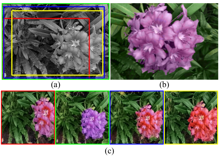
Figure 3: Our query-based injection strategy could generate plausible results from inconsistent colors. (a) is the input monochromatic image with different sampled patches (denoted as rectangles); (b) is the final output of our model with consistent color; (c) are the results from CT² (Weng et al. 2022), corresponding to image patches in (a).

Luminance and density representation

We first construct the representation for luminance and density, and then fix them during color representation prediction. The luminance and density representation can be simply defined as:

$$l=\Theta_{\mathrm{M}}(\mathbf{w},\mathbf{d}),$$ (7)

where $l$ is the rendered monochromatic output, $\Theta_{\mathrm{M}}(\cdot,\cdot)$ is the mapping network in luminance and density representation. COLMAP (Schönberger and Frahm 2016; Schönberger et al. 2016) is used for pose estimation during mapping defined by Eq. (7). Due to that COLMAP’s proper functioning requires monochromatic images, our setting does not affect its performance. We first supervise the luminance and density representation using photometric loss similar to Eq. (5),

$$\mathcal{L}_{\mathrm{photometric}}=\sum_{\mathbf{p}\in\mathcal{P}}||\mathbf{L}_{\mathcal{P}}(\mathbf{p})-\hat{\mathbf{L}}_{\mathcal{P}}(\mathbf{p})||^{2}_{2},$$ (8)

where $\mathbf{p}=p(\mathbf{r})$ is the pixel corresponding to the ray $\mathbf{r}$.

Color representation prediction

With the luminance and density representation obtained in Eq. (7), we aim at predicting the color representation via the mapping network $\Theta_{\mathrm{Z}}(\cdot,\cdot)$ below,

$$\mathbf{z}=\Theta_{\mathrm{Z}}(\mathbf{w},\mathbf{d}),$$ (9)

where $\mathbf{z}$ denotes the predicted representation for $ab$ channels. The difficulty encountered by the mapping correlation in Eq. (9) comes from the lack of color supervision during representation construction. Thus, incorporating color knowledge into predicted representation, while preserving the plausibility and vividness of the results, is crucial.

Query-based colorization.

Our approach could utilize color information from different off-the-shelf colorization models. Without losing generality, we obtain color knowledge from a state-of-the-art automatic colorization work CT² (Weng et al. 2022). For maintaining higher plausibility, rather than colorizing images ahead of representation prediction (i.e, the “colorize-then-fuse” paradigm), where each image pixel in a camera pose is assigned with a fixed color before optimization, we propose a query-based colorization strategy by first querying the colorization module with the rendered luminance samples and then dynamically injecting color knowledge into the predicted representation. Such a query strategy colorizes each pixel in a camera pose multiple times and incorporates various possible colors into our color representation. As displayed in Fig. 3, though the sampled image patches in one image are assigned with different colors during each iteration (Fig. 3(c)), such seeming variation can in turn help to reach plausible and consistent results by averaging over different colors (Fig. 3(b)).

Our query-based colorization can be conducted in a simple way. After sampling each batch of rays corresponding to image patch $\mathcal{P}(\mathbf{u},s)$, we first render the monochromatic image patch $\hat{\mathbf{L}}_{\mathcal{P}}$ based on the luminance and density representation. Then we colorize this monochromatic image patch by feeding it into the colorization module as follows:

$$\mathbf{B}_{\mathcal{P}}=\mathcal{F}(\hat{\mathbf{L}}_{\mathcal{P}}),$$ (10)

where $\mathcal{F}(\cdot)$ denotes the colorization module and $\mathbf{B}_{\mathcal{P}}$ denotes the colorized image patch.

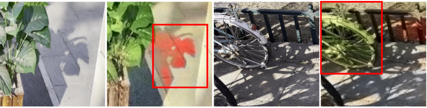
Figure 4: Outliers from colorized image patches. For both examples, the left is the reference image and the right is the colorized image with outliers, marked by red rectangles.

Histogram-guided purification.

The query-based colorization has been able to produce plausible colorized samples across different views. However, due to incorrect understanding of the scene, the colorization module sometimes yield outliers with different layout or illumination that may undermine the colorization process, demonstrated in Fig. 4.

We propose to purify such outliers by histogram similarity comparison. Before training, we sample patches with $s=0.7$ and generate base color images $\mathbf{b}$. With large perceptual field, $\mathbf{b}$ capture full semantics of the scene, so few outliers occur. In the training epochs, we sample $\mathcal{P}$ with $s\in[0.3,0.7]$ to colorize the details. After acquiring the colorized patches $\mathbf{B}_{\mathcal{P}}$, we calculate the histogram similarity between $\mathbf{B}_{\mathcal{P}}$ and $\mathbf{b}$:

$$d(\mathbf{B}_{\mathcal{P}})=\frac{\sum_{j}(\Delta_{H}(\mathbf{b})\odot\Delta_{H}(\mathbf{B}_{\mathcal{P}}))}{\sqrt{\sum_{j}(\Delta_{H}(\mathbf{b}))^{2}\cdot\sum_{j}(\Delta_{H}(\mathbf{B}_{\mathcal{P}}))^{2}}},$$ (11)

where $\odot$ denotes element-wise multiplication and $\Delta_{H}(\cdot)$ is the normalized color histogram of a given image. $j$ is histogram bin index.

As demonstrated in Fig. 2, by comparing $\Delta_{H}(\mathbf{B}_{\mathcal{P}})$ with $\Delta_{H}(\mathbf{b})$, the purification module can exclude outliers deviating from samples based on the selection scheme as follows:

$$\mathcal{H}(\mathbf{B}_{\mathcal{P}})=\left\{\begin{array}[]{rc}1,&\mathop{\max}(d(\mathbf{B}_{\mathcal{P}}))>T,\\ 0,&\mathrm{otherwise}.\end{array}\right.$$ (12)

We empirically choose $5$ base images with $T=0.80$ in our experiments, $\mathop{\max}(d(\mathbf{B}_{\mathcal{P}}))$ denotes the highest similarity score with the base images. The histogram-guided purification is formulated as $\mathbf{Y}_{\mathcal{P}}=\mathcal{H}(\mathbf{B}_{\mathcal{P}})\odot\mathbf{B}_{\mathcal{P}}$, where $\mathbf{Y}_{\mathcal{P}}$ denotes the purified color image patches. With ample plausible color information, we further propose a color injection module, aiming to produce vivid results by properly injecting $\mathbf{Y}_{\mathcal{P}}$ to the color representation $\Theta_{\mathrm{Z}}$.

Classification-based color injection.

The color injection can be achieved by minimizing the photometric loss similar to Eq. (5), which transfers color information from the colorization module to the predicted representation by measuring the differences in their output. Despite the effectiveness of photometric loss in reconstructing radiance fields, it is incapable of producing vivid color (Zhang, Isola, and Efros 2016), since the extensive color distribution inevitably collapses into its mean value during the computation of photometric loss, which renders grayish and less vivid samples from predicted representations.

We propose to preserve extensive color distribution by considering color injection as a classification task. To fit the classification objective, we first quantize the possible $ab$ space with grid size 10 and keep $Q=313$ colors which are in-gamut, denoted as $\omega_{q}\in\mathbb{R}^{2}$, where $q\in\{1,2,\ldots,Q\}$ is the index of quantized $ab$ candidates. We change the output channel of the color representation $\Theta_{Z}(\cdot)$ to $Q$ channels as probability scores of the possible color labels. For each sampling patch $\mathcal{P}$, we predict a probability distribution of quantized $ab$ colors, denoted as $\hat{\mathbf{Z}}_{\mathcal{P}}\in[0,1]^{K\times K\times Q}$.

To supervise $\hat{\mathbf{Z}}_{\mathcal{P}}$ with $\mathbf{Y}_{\mathcal{P}}$, for each pixel $\mathbf{p}$, we find $5$ quantized colors closest to $\mathbf{Y}_{\mathcal{P}}(\mathbf{p})$ using the nearest neighbor algorithm, and use their distances as weights to generate the soft label $\mathbf{Z}_{\mathcal{P}}(\mathbf{p})$, such soft-label operation is denoted as $\mathcal{S}(\cdot)$, i.e, $\mathbf{Z}_{\mathcal{P}}(\mathbf{p})=\mathcal{S}(\mathbf{Y}_{\mathcal{P}}(\mathbf{p}))$.

We formulate the color classification loss as follows:

$$\mathcal{L}_{\mathrm{cl}}=-\!\!\!\sum_{\mathbf{p}\in\mathcal{P},q}\!\!(\log(\hat{\mathbf{Z}}_{\mathcal{P}}^{q}(\mathbf{p}))-\log(\mathbf{Z}_{\mathcal{P}}^{q}(\mathbf{p}))\mathbf{Z}_{\mathcal{P}}^{q}(\mathbf{p}).$$ (13)

In the inference stage, we simply choose the color with the largest possibility score from $Q$ candidates, and take the $ab$ values of that color as our prediction:

$$\hat{\mathbf{Y}}_{\mathcal{P}}(\mathbf{p})=\mathbf{\omega}_{q},\mathrm{where}\,\,q=\mathop{\arg\max}\limits_{q}\,\hat{\mathbf{Z}}_{\mathcal{P}}^{q}(\mathbf{p}),$$ (14)

and $\mathbf{Z}_{\mathcal{P}}^{q}(\mathbf{p})$ is the probability score for $\omega_{q}$ color. We formulate the final results in RGB channel (denoted as $\hat{\mathbf{C}}_{\mathcal{P}}$) by concatenating $\hat{\mathbf{Y}}_{\mathcal{P}}$ with $\hat{\mathbf{L}}_{\mathcal{P}}$ and converting the output from $Lab$ to RGB color space: $\hat{\mathbf{C}}_{\mathcal{P}}=\mathrm{Lab2RGB}(\mathrm{concat}\{\hat{\mathbf{L}}_{\mathcal{P}},\hat{\mathbf{Y}}_{\mathcal{P}}\}).$

Implementation details

We implement our pipeline using PyTorch. We integrate the colorization modules based on their released implementation, and freeze their model weights along training. Following the design in NeRF (Mildenhall et al. 2020), an eight-layer MLP with 256 channels is used for points encoding, and the luminance and color MLPs have two layers with 128 channels for directional encoding. Along each ray, we sample 64 points to train a “coarse” network and 64 additional importance sampling points to train a “fine” network. An image patch with $K=128$ size is sampled in a batch. Positional encoding is applied to input location and direction similar to NeRF (Mildenhall et al. 2020). We optimize our model for 30 epochs on one NVIDIA TITAN RTX GPU.

Table 1: Quantitative comparison results on synthetic monochromatic data. $\uparrow$ ($\downarrow$) means higher (lower) is better. The best performances are highlighted in bold.

Category	Method	PSNR$\uparrow$	SSIM$\uparrow$	LPIPS$\downarrow$	Colorful$\uparrow$	$\Delta$ Colorful$\downarrow$
Comparison	Vid (Lei and Chen 2019)+NeRF	17.78	0.63	0.31	12.88	23.59
Comparison	ARF (Zhang et al. 2022)	17.82	0.54	0.37	36.33	N/A
Comparison	CLIP-NeRF (Wang et al. 2022a)	17.76	0.76	0.31	30.92	12.18
Comparison	CT2 (Weng et al. 2022)+NeRF	18.90	0.80	0.32	48.52	18.24
Ablation	w/o histogram-guided purification	17.74	0.77	0.25	54.41	19.20
Ablation	w/o classification-based color injection	19.22	0.81	0.22	49.28	12.82
Ours	ColorNeRF	20.76	0.81	0.21	55.40	12.15

Experiments

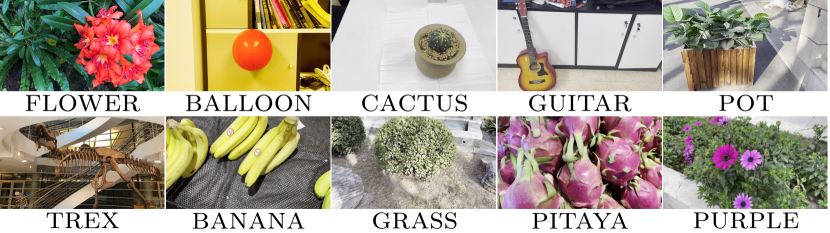
Figure 5: One image sample for each scene in our dataset. The names of the scenes are listed below the image.

Dataset.

To conduct quantitative evaluation, we first employ synthetic monochromatic data. Two samples from the conventional LLFF dataset (Mildenhall et al. 2019) are employed (flower and trex). We additionally capture 8 scenes by following the instructions of LLFF (Mildenhall et al. 2019), and each scene consists of $30$ to $50$ viewpoints. A sample of each scene can be found in Fig. 5. During the experiments, the samples in the above scenes are transformed into their monochromatic counterparts, and their original colorful version is used as the ground truth. To evaluate whether ColorNeRF is effective for real monochromatic data (without ground truth color) directly produced by imaging devices. We further capture a scene using the spike camera, a novel type of neuromorphic sensor recording scene radiance as colorless neural spikes, which can be integrated to monochromatic images (Huang et al. 2022). In addition, two multi-view scenes collected from old movies are employed to demonstrate our potential in rejuvenating old digital archives. All scenes are first processed by COLMAP (Schönberger and Frahm 2016; Schönberger et al. 2016) for pose estimation. Synthetic data are used for quantitative and qualitative evaluations.

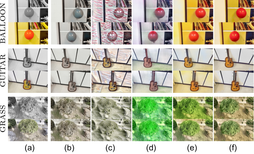
Figure 6: Qualitative comparison with selected baselines. In each scene, (a) is the monochormatic input and reference image (not used in training); (b-f) show two novel synthesised views of the compared methods. (b): Vid (Lei and Chen 2019) + NeRF; (c): ARF (Zhang et al. 2022); (d): CLIP-NeRF (Wang et al. 2022a); (e): CT² (Weng et al. 2022)+NeRF; (f) ColorNeRF (ours).

Baselines.

We compare ColorNeRF against the following baselines: 1) CLIP-NeRF (Wang et al. 2022a), a 3D object manipulation method with color editing ability; 2) ARF (Zhang et al. 2022), a style transfer NeRF method using a ground truth image as the reference style image; 3) CT² (Weng et al. 2022)+NeRF, results using the “colorize-then-fuse” paradigm with the same colorization model CT² (Weng et al. 2022) used in our pipeline; 4) Vid (Lei and Chen 2019)+NeRF, results using the “colorize-then-fuse” paradigm with state-of-the-art automatic video colorization work (Lei and Chen 2019). We do not compare with palette-based color editing NeRFs (Tojo and Umetani 2022), since their palette extraction module (Tan, Echevarria, and Gingold 2018; Tan, Lien, and Gingold 2017) could not extract palette from monochromatic images.

Error metrics.

We measure the performance of our colorized results following the conventionally used metrics in colorization and implicit radiance fields. PSNR (Huynh-Thu and Ghanbari 2008), SSIM (Wang et al. 2004) and LPIPS (Zhang et al. 2018) are used to measure the image quality of the results; Colorful Score (Hasler and Süsstrunk 2003) reflects the vividness of the colorized images. The absolute colorfulness score difference ($\Delta$ Colorful) of the ground truth images and predicted ones could also show how close predictions are to ground truth in terms of vividness.

While pixel-level metrics, such as PSNR and SSIM, are commonly utilized for quantitative evaluation, it has been recognized that these metrics may not accurately reflect the true performance of colorization techniques (Messaoud, Forsyth, and Schwing 2018; Su, Chu, and Huang 2020; Wu et al. 2021). Hence, in order to validate the performance of the compared methods, a user study is conducted.

Quantitative experiments.

The quantitative results on synthetic monochromatic data are reported in Table 1. Our model achieves better performance in all metrics. CT² (Weng et al. 2022)+NeRF has the second-best performance, but their major drawbacks lie in the inconsistency observed in Fig. 6. ARF (Zhang et al. 2022) utilizes a ground truth image as the style image, hence it is unsuitable to compare with other methods on colorfulness metrics.

Novel view synthesis.

In Fig. 6, we show the novel view synthesis results on our model and the compared baselines. It is clear that our model could yield the most plausible and vivid colorization results. In Vid (Lei and Chen 2019)+NeRF, the video colorization module fails to colorize vivid results, probably due to it is over-fitted on its training dataset and has a major domain gap with real-world custom scenes. ARF (Zhang et al. 2022) focuses mainly on extracting the pattern in the style image, it could get artistic results, but the results are not plausible since the geometry of the scenes are influenced by the style patterns. CLIP-NeRF (Wang et al. 2022a) could not extract color information from monochromatic images. Hence it yields less vivid results. In CT² (Weng et al. 2022)+NeRF, the results are not plausible since the color is flickering when the view direction changes. We refer the readers to the project page for more comprehensive results in our dataset with higher resolution and more synthesised views.

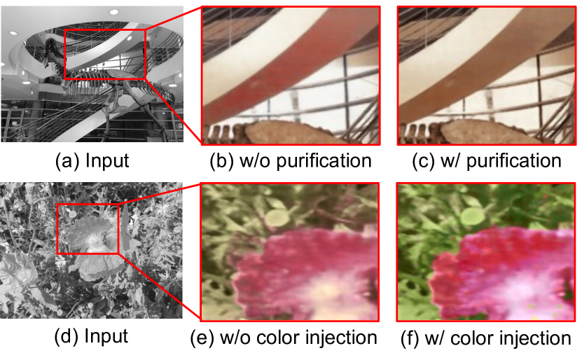
Figure 7: Ablation study. Comparison between (b) and (c) shows the histogram-guided purification module could purify undesired color; comparison between (e) and (f) exhibits the classification-based color injection module produces more vivid outputs.

Table 2: User study results. Higher score means better performance, and the best scores are highlighted in bold. Our model exhibits superior performance in terms of plausibility and vividness compared to other methods. (a): Vid (Lei and Chen 2019)+NeRF; (b): ARF (Zhang et al. 2022); (c): CLIP-NeRF (Wang et al. 2022a); (d): CT² (Weng et al. 2022)+NeRF; (e): ColorNeRF (ours).

Method	(a)	(b)	(c)	(d)	(e)
Plausibility	1.70	2.23	3.10	3.25	4.26
Vividness	3.00	2.35	2.55	3.40	4.67

Ablation study.

The quantitative and qualitative ablation results are presented in Table 1 and Fig. 7, respectively. The absence of the histogram-based purification module in quantitative experiments results in a high Colorful score, but the $\Delta$ Colorful score is also high, indicating the presence of undesired colors, such as the red area in Fig. 7(b). On the other hand, the omission of the classification-based color injection in the ablation experiments leads to a decrease in the Colorful score, indicating a less vivid performance, e.g., the yellowish leaves in Fig. 7(e).

User study.

In addition to quantitative and qualitative comparisons, we conduct user study experiments to assess whether our results are preferred by human observers. The experiment set is composed of the 10 scenes in synthetic monochromatic data. For each scene, we provide 3 synthesised novel views colorized by 5 different methods: Vid (Lei and Chen 2019)+NeRF, ARF (Zhang et al. 2022), CLIP-NeRF (Wang et al. 2022a), CT² (Weng et al. 2022)+NeRF and Ours. Participants are asked to score 1-5 (higher means better performance) on the results in terms of plausibility and vividness. The order of displayed methods is shuffled in each scene. Each experiment is completed by 50 participants. Results in Table 2 show our method outperforms other methods in terms of plausibility and vividness.

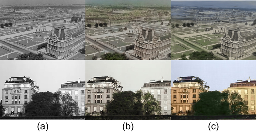
Figure 8: Qualitative comparison with Vid (Lei and Chen 2019) + NeRF on two old movie clips. (a): input; (b): Vid (Lei and Chen 2019) + NeRF; (c): ColorNeRF (ours). Please refer to the project page for animation results.

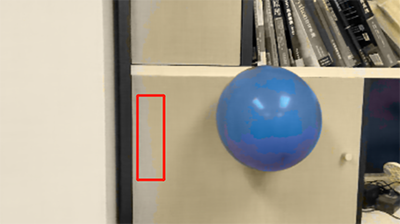
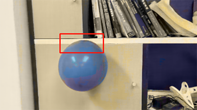
Figure 9: Three novel views of ColorNeRF using color information from L-CoDer (Chang et al. 2022) on balloon scene are shown. The text guidance used in L-CoDer is “Blue balloon on white wall”.

Results on real data.

We show the results of our model on real monochromatic data in Fig. 8, which also demonstrate our model’s applications on creating colors for rejuvenating old digital archives in the form of radiance fields.

Conclusions

In this paper, we introduce ColorNeRF, a novel approach capable of generating plausible and vivid radiance fields from monochromatic images. Our approach employs a representation prediction framework, incorporating a query-based colorization module, a histogram-guided purification module, and a classification-based color injection module, to ensure the plausibility and vividness of the results. Extensive experiments are conducted to validate the advantages and broad applications of our model.

Limitations and future work.

Theoretically, an arbitrary colorization network could be incorporated with ColorNeRF. In Fig. 9, we show the novel views generated by ColorNeRF using language-guided colorization model L-CoDer (Chang et al. 2022). Although our model produces plausible and vivid outcomes, there are some undesired artifacts in the results. This is resulted from the inferior performance of L-CoDer (Chang et al. 2022) under cases with uncertain background colors, which also demonstrates that the effectiveness of ColorNeRF is contingent upon the performance of the external colorization module. The advancement of 2D colorization models is expected to mitigate this issue by generating more plausible results.

References

- Anwar et al. (2020) Anwar, S.; Tahir, M.; Li, C.; Mian, A.; Khan, F. S.; and Muzaffar, A. W. 2020. Image colorization: A survey and dataset. arXiv preprint arXiv:2008.10774.
- Cao et al. (2017) Cao, Y.; Zhou, Z.; Zhang, W.; and Yu, Y. 2017. Unsupervised diverse colorization via generative adversarial networks. In Machine Learning and Knowledge Discovery in Databases: European Conference.
- Chang et al. (2022) Chang, Z.; Weng, S.; Li, Y.; Li, S.; and Shi, B. 2022. L-CoDer: Language-based colorization with color-object decoupling transformer. In Proc. of European Conference on Computer Vision.
- Chen et al. (2018) Chen, J.; Shen, Y.; Gao, J.; Liu, J.; and Liu, X. 2018. Language-based image editing with recurrent attentive models. In Proc. of Computer Vision and Pattern Recognition.
- Cheng, Yang, and Sheng (2015) Cheng, Z.; Yang, Q.; and Sheng, B. 2015. Deep colorization. In Proc. of International Conference on Computer Vision.
- Fan et al. (2022) Fan, Z.; Wang, P.; Jiang, Y.; Gong, X.; Xu, D.; and Wang, Z. 2022. NeRF-SOS: Any-view self-supervised object segmentation on complex scenes. CoRR, abs/2209.08776.
- Geonung et al. (2022) Geonung, K.; Kyoungkook, K.; Seongtae, K.; Hwayoon, L.; Sehoon, K.; Jonghyun, K.; Seung-Hwan, B.; and Sunghyun, C. 2022. BigColor: Colorization using a generative color prior for natural images. In Proc. of European Conference on Computer Vision.
- Gong et al. (2023) Gong, B.; Wang, Y.; Han, X.; and Dou, Q. 2023. RecolorNeRF: Layer decomposed radiance fields for efficient color editing of 3D scenes. Proc. of ACM International Conference on Multimedia.
- Guadarrama et al. (2017) Guadarrama, S.; Dahl, R.; Bieber, D.; Shlens, J.; Norouzi, M.; and Murphy, K. 2017. PixColor: Pixel recursive colorization. In Proc. of British Machine Vision Conference.
- Hasler and Süsstrunk (2003) Hasler, D.; and Süsstrunk, S. 2003. Measuring colorfulness in natural images. In Human Vision and Electronic Imaging VIII.
- Huang et al. (2022) Huang, T.; Zheng, Y.; Yu, Z.; Chen, R.; Li, Y.; Xiong, R.; Ma, L.; Zhao, J.; Dong, S.; Zhu, L.; et al. 2022. 1000 faster camera and machine vision with ordinary devices. Engineering.
- Huang, Zhao, and Liao (2022) Huang, Z.; Zhao, N.; and Liao, J. 2022. Unicolor: A unified framework for multi-modal colorization with transformer. ACM Transactions on Graphics.
- Huynh-Thu and Ghanbari (2008) Huynh-Thu, Q.; and Ghanbari, M. 2008. Scope of validity of PSNR in image/video quality assessment. Electronics letters.
- Iizuka, Simo-Serra, and Ishikawa (2016) Iizuka, S.; Simo-Serra, E.; and Ishikawa, H. 2016. Let there be color!: Joint end-to-end learning of global and local image priors for automatic image colorization with simultaneous classification. ACM Transactions on Graphics.
- Ironi, Cohen-Or, and Lischinski (2005) Ironi, R.; Cohen-Or, D.; and Lischinski, D. 2005. Colorization by example. Rendering techniques.
- Kobayashi, Matsumoto, and Sitzmann (2022) Kobayashi, S.; Matsumoto, E.; and Sitzmann, V. 2022. Decomposing NeRF for editing via feature field distillation. In Proc. of Neural Information Processing Systems.
- Kuang et al. (2022) Kuang, Z.; Luan, F.; Bi, S.; Shu, Z.; Wetzstein, G.; and Sunkavalli, K. 2022. PaletteNeRF: Palette-based appearance editing of neural radiance fields. Proc. of Computer Vision and Pattern Recognition.
- Larsson, Maire, and Shakhnarovich (2016) Larsson, G.; Maire, M.; and Shakhnarovich, G. 2016. Learning representations for automatic colorization. In Proc. of European Conference on Computer Vision.
- Lei and Chen (2019) Lei, C.; and Chen, Q. 2019. Fully automatic video colorization with self-regularization and diversity. In Proc. of Computer Vision and Pattern Recognition.
- Levin, Lischinski, and Weiss (2004) Levin, A.; Lischinski, D.; and Weiss, Y. 2004. Colorization using optimization. Proc. of ACM SIGGRAPH.
- Liu et al. (2021) Liu, S.; Zhang, X.; Zhang, Z.; Zhang, R.; Zhu, J.-Y.; and Russell, B. 2021. Editing conditional radiance fields. arXiv:2105.06466.
- Luan et al. (2007) Luan, Q.; Wen, F.; Cohen-Or, D.; Liang, L.; Xu, Y.-Q.; and Shum, H.-Y. 2007. Natural image colorization. In Proceedings of the 18th Eurographics conference on Rendering Techniques.
- Ma et al. (2022) Ma, L.; Li, X.; Liao, J.; Zhang, Q.; Wang, X.; Wang, J.; and Sander, P. V. 2022. Deblur-NeRF: Neural radiance fields from blurry images. In Proc. of Computer Vision and Pattern Recognition.
- Martin-Brualla et al. (2021) Martin-Brualla, R.; Radwan, N.; Sajjadi, M. S. M.; Barron, J. T.; Dosovitskiy, A.; and Duckworth, D. 2021. NeRF in the Wild: Neural radiance fields for unconstrained photo collections. In Proc. of Computer Vision and Pattern Recognition.
- Messaoud, Forsyth, and Schwing (2018) Messaoud, S.; Forsyth, D.; and Schwing, A. G. 2018. Structural consistency and controllability for diverse colorization. In Proc. of European Conference on Computer Vision.
- Mildenhall et al. (2019) Mildenhall, B.; Srinivasan, P. P.; Ortiz-Cayon, R.; Kalantari, N. K.; Ramamoorthi, R.; Ng, R.; and Kar, A. 2019. Local light field fusion: Practical view synthesis with prescriptive sampling guidelines. ACM Transactions on Graphics.
- Mildenhall et al. (2020) Mildenhall, B.; Srinivasan, P. P.; Tancik, M.; Barron, J. T.; Ramamoorthi, R.; and Ng, R. 2020. NeRF: Representing scenes as neural radiance fields for view synthesis. In Proc. of European Conference on Computer Vision.
- Niemeyer and Geiger (2021) Niemeyer, M.; and Geiger, A. 2021. GIRAFFE: Representing scenes as compositional generative neural feature Fields. In Proc. of Computer Vision and Pattern Recognition.
- Pearl, Treibitz, and Korman (2022) Pearl, N.; Treibitz, T.; and Korman, S. 2022. NAN: Noise-aware NeRFs for burst-denoising. In Proc. of Computer Vision and Pattern Recognition.
- Schönberger and Frahm (2016) Schönberger, J. L.; and Frahm, J.-M. 2016. Structure-from-motion revisited. In Proc. of Computer Vision and Pattern Recognition.
- Schönberger et al. (2016) Schönberger, J. L.; Zheng, E.; Pollefeys, M.; and Frahm, J.-M. 2016. Pixelwise view selection for unstructured multi-view stereo. In Proc. of European Conference on Computer Vision.
- Schwarz et al. (2020) Schwarz, K.; Liao, Y.; Niemeyer, M.; and Geiger, A. 2020. GRAF: Generative radiance fields for 3D-aware image synthesis. In Proc. of Neural Information Processing Systems.
- Su, Chu, and Huang (2020) Su, J.-W.; Chu, H.-K.; and Huang, J.-B. 2020. Instance-aware image colorization. In Proc. of Computer Vision and Pattern Recognition.
- Tan, Echevarria, and Gingold (2018) Tan, J.; Echevarria, J. I.; and Gingold, Y. I. 2018. Efficient palette-based decomposition and recoloring of images via RGBXY-space geometry. ACM Transactions on Graphics.
- Tan, Lien, and Gingold (2017) Tan, J.; Lien, J.; and Gingold, Y. I. 2017. Decomposing images into layers via RGB-space geometry. ACM Transactions on Graphics.
- Tojo and Umetani (2022) Tojo, K.; and Umetani, N. 2022. Recolorable posterization of volumetric radiance fields using visibility-weighted palette extraction. Computer Graphics Forum.
- Vitoria, Raad, and Ballester (2020) Vitoria, P.; Raad, L.; and Ballester, C. 2020. ChromaGAN: Adversarial picture colorization with semantic class distribution. In Proc. of IEEE Winter Conference on Applications of Computer Vision.
- Wang et al. (2022a) Wang, C.; Chai, M.; He, M.; Chen, D.; and Liao, J. 2022a. CLIP-NeRF: Text-and-image driven manipulation of neural radiance fields. In Proc. of Computer Vision and Pattern Recognition.
- Wang et al. (2022b) Wang, C.; Jiang, R.; Chai, M.; He, M.; Chen, D.; and Liao, J. 2022b. NeRF-Art: Text-driven neural radiance fields stylization. arXiv preprint arXiv:2212.08070.
- Wang et al. (2004) Wang, Z.; Bovik, A. C.; Sheikh, H. R.; and Simoncelli, E. P. 2004. Image quality assessment: from error visibility to structural similarity. IEEE Transactions on Image Processing.
- Weng et al. (2022) Weng, S.; Sun, J.; Li, Y.; Li, S.; and Shi, B. 2022. CT: Colorization transformer via color tokens. In Proc. of European Conference on Computer Vision.
- Wu et al. (2021) Wu, Y.; Wang, X.; Li, Y.; Zhang, H.; Zhao, X.; and Shan, Y. 2021. Towards vivid and diverse image colorization with generative color prior. In Proc. of International Conference on Computer Vision.
- Yun et al. (2023) Yun, J.; Lee, S.; Park, M.; and Choo, J. 2023. iColoriT: Towards propagating local hints to the right region in interactive colorization by leveraging vision transformer. In Proc. of IEEE Winter Conference on Applications of Computer Vision.
- Zhang et al. (2022) Zhang, K.; Kolkin, N.; Bi, S.; Luan, F.; Xu, Z.; Shechtman, E.; and Snavely, N. 2022. ARF: Artistic radiance fields. In Proc. of European Conference on Computer Vision.
- Zhang, Isola, and Efros (2016) Zhang, R.; Isola, P.; and Efros, A. A. 2016. Colorful image colorization. In Proc. of European Conference on Computer Vision.
- Zhang et al. (2018) Zhang, R.; Isola, P.; Efros, A. A.; Shechtman, E.; and Wang, O. 2018. The unreasonable effectiveness of deep features as a perceptual metric. In Proc. of Computer Vision and Pattern Recognition.
- Zhang et al. (2017) Zhang, R.; Zhu, J.-Y.; Isola, P.; Geng, X.; Lin, A. S.; Yu, T.; and Efros, A. A. 2017. Real-time user-guided image colorization with learned deep priors. ACM Transactions on Graphics.
- Zhao et al. (2020) Zhao, J.; Han, J.; Shao, L.; and Snoek, C. G. 2020. Pixelated semantic colorization. International Journal of Computer Vision.