Second-order flows for approaching stationary points of a class of non-convex energies via convex-splitting schemes

Abstract

The use of accelerated gradient flows is an emerging field in optimization, scientific computing and beyond. This paper contributes to the theoretical underpinnings of a recently-introduced computational paradigm known as second-order flows, which demonstrate significant performance particularly for the minimization of non-convex energy functionals defined on Sobolev spaces, and are characterized by novel dissipative hyperbolic partial differential equations. Our approach hinges upon convex-splitting schemes, a tool which is not only pivotal for clarifying the well-posedness of second-order flows, but also yields a versatile array of robust numerical schemes through temporal and spatial discretization. We prove the convergence to stationary points of such schemes in the semi-discrete setting. Further, we establish their convergence to time-continuous solutions as the time-step tends to zero, and perform a comprehensive error analysis in the fully discrete case. Finally, these algorithms undergo thorough testing and validation in approaching stationary points of non-convex variational models in applied sciences, such as the Ginzburg-Landau energy in phase-field modeling and a specific case of the Landau-de Gennes energy of the Q-tensor model for liquid crystals.

Keywords: non-convex functional, second-order flow, dissipative hyperbolic equation, convex-splitting scheme, error analysis, Ginzburg-Landau energy, Landau-de Gennes model

2020 Mathematics Subject Classification: 35Q90, 35L71, 65M15, 65K10

1 Introduction

Second-order flows is a concept proposed in [11], referring to certain dissipative second-order hyperbolic PDEs, which serves as a compelling alternative to gradient flows for approaching minimizers of variational problems. (Non-convex) variational models and partial differential equations (PDEs) are central topics in scientific computing and applied mathematics, offering useful mathematical tools to describe a variety of complex phenomena across multiple disciplines. The current paper is motivated to develop robust and efficient optimization methods based on second-order flows for a class of non-convex variational problems, e.g., the Ginzburg-Landau energy in phase-field modelings and the Landau-de Gennes energy of the Q-tensor model for liquid crystals.

These variational models, while distinct in their physical contexts and implications, are grounded in a common mathematical framework. Let $H$ be a Hilbert space of the vector-valued function $\mathbf{u}:\Omega\subset\mathbb{R}^{d}\rightarrow\mathbb{R}^{N}(d=1,2,3)$, where $\Omega$ is a bounded domain. The goal is to find a function $\mathbf{u}_{g}\in H$ that minimizes an energy functional $E$, formulated as

$$E_{g}:=E(\mathbf{u}_{g})=\min_{\mathbf{u}\in H}E(\mathbf{u}),$$ (1.1)

with the energy functional given by

$$E(\mathbf{u})=\int_{\Omega}\left(\frac{1}{2}|\nabla\mathbf{u}|^{2}+F(\mathbf{u})\right)\,d\mathbf{x},$$ (1.2)

where $\nabla$ denotes the gradient operator, and $|\nabla\mathbf{u}|^{2}=\sum_{i=1}^{N}\sum_{j=1}^{d}\left(\frac{\partial u_{i}}{\partial x_{j}}\right)^{2}$. This paper focuses on a typical nonlinear potential $F$ of the form

$$F(\mathbf{u})=\frac{\alpha}{4}|\mathbf{u}|^{4}-\frac{\beta}{2}|\mathbf{u}|^{2}+\gamma$$

with constants $\alpha,\beta,\gamma$ all positive. The associated Euler-Lagrange equation for this variational problem is

$$-\Delta\mathbf{u}+f(\mathbf{u})=0\quad\text{in }\Omega,$$ (1.3)

where $\Delta\mathbf{u}$ represents the Laplacian of $\mathbf{u}$, and $f(\mathbf{u})=\alpha|\mathbf{u}|^{2}\mathbf{u}-\beta\mathbf{u}$ is derived from the variation of the nonlinear potential term $F(\mathbf{u})$. The boundary conditions for the equation (1.3) are determined by the specific characterization of the space $H$ and the nature of the domain $\Omega$. The existence of a minimizer is a straightforward exercise using the direct method in the calculus of variations, see, e.g., [46].

Gradient flow methods have been quite popular to tackle this type of problems [18, 19, 33, 34, 31, 10], owing to their obvious advantages: (i) only the gradient information (or first-order variational derivative) of the objective functional $E(\mathbf{u})$ is required, which enables easy implementation through various discretization strategies; (ii) the energy stability is often preserved due to the dissipative mechanism. Notably, employing the $L^{2}$-gradient flow of the energy (1.2) leads to the derivation of a parabolic equation, which can be expressed as:

$$\partial_{t}\mathbf{u}=\Delta\mathbf{u}-f(\mathbf{u}),\quad\text{for }\mathbf{x}\in\Omega,\,t>0,$$ (1.4)

subject to suitable boundary conditions on $\partial\Omega\times\{t\,|\,t\geq 0\}$. This equation is reminiscent of the well-known Allen-Cahn equation, a representative equation of phase field type models. The Allen-Cahn equation arises from standard energetic variational approaches, e.g. the Onsager maximum dissipation principle, primarily to describe the evolution of phase transitions and interfacial dynamics in materials science [2, 13, 12, 39, 40]. We would like to point out that the use of Allen-Cahn equation in modeling real-world phase transitions differs from its application as a computational strategy for solving energy minimization problems. Another note is that, the adoption of the $H^{-1}$-gradient flow for the same energy functional, given its inherent property of mass (concentration) preservation, leads to a different setting compared to the $L^{2}$ gradient flow. While our primary focus in this work remains on the $L^{2}$-metric gradients of energy functionals, the general methodology may be analogous to gradients with other metric in energy minimization.

The idea of second-order flows is rooted in a recent topic in convex optimization. Considering some cost function $J:H\to\mathbb{R}$ for minimization, second-order dynamics of the following type have been of high interest in the literature [20, 47, 4, 3]

$$\ddot{\mathbf{u}}+\eta(t)\dot{\mathbf{u}} =-\nabla J(\mathbf{u}),$$ (1.5)

where $\eta(t)>0$ is a damping coefficient. When $J(\mathbf{u})$ is a convex function over finite dimensional spaces, i.e., (1.5) is a system of ordinary differential equations (ODEs), such a formulation is known to offer distinct advantages referring to the recent progress of second-order inertial dynamics in optimization. This was mainly sparked by the work of Su et al. [47], which established a connection between second-order ODEs and Nesterov’s accelerated gradient method [37]. Subsequent research, including studies [4, 55, 38, 9, 3], has continued to explore the theoretical and practical aspects of these second-order ODEs. In this work we focus on second-order flows particular for the PDE cases. The study of second-order flows faces additional complexities, particularly in their theoretical understanding and numerical analysis, due to the fact that $\nabla J(\mathbf{u})$ involves spatial differential operators, see, e.g., [16]. In a recent work [11], the authors have introduced two distinct types of second-order flows as strategies for minimizing a constrained non-convex energy given by the Gross-Pitaevskii functional, which is a fundamental model for simulating the ground states of rotating Bose-Einstein condensates (BECs). The newly introduced second-order flow methods, incorporating both explicit and semi-implicit temporal discretizations, have demonstrated notable improvements over gradient flow type approaches in terms of computational efficiency.

Investigating the analytical aspects, numerical methods, and application of second-order flows for (non-convex) variational problems offers an intriguing and largely unexploited area of research. Despite some of the initial treatment as explored in [16], and progress on numerical efficiency made in the previous work [11], a comprehensive theoretical and numerical understanding of second-order flows, especially in the context of non-convex variational problems, remains a challenging open topic. That motivates the current work, where we try to go one step further towards non-convex variational problems with second-order flows. In particular, we wish to establish some foundations for their numerical analysis and convergence to stationary points. A full convergence analysis is particularly challenging with non-convex energies, where even in the finite-dimensional setting the use of some form of Łojasiewicz-type inequalities is required [8]. In the PDE setting, the adequate notion is that of Łojasiewicz-Simon inequalities, which were first introduced in [44] and have been applied to semilinear second-order dissipative equations in [27], among others. However, for the specific energies (1.2) that we consider here, the vectorial setting and strength of the nonlinearities prevent such methods from being directly applicable.

When taking $H=H_{0}^{1}(\Omega,\mathbb{R}^{N})$ and formulating a second-order flow to approach a minimizer or stationary point of $E(\mathbf{u})$ in (1.2), we are led to the following dissipative hyperbolic PDE:

$$\partial_{tt}\mathbf{u}+\eta(t)\partial_{t}\mathbf{u} =\Delta\mathbf{u}-f(\mathbf{u}),\quad x\in\Omega,\,t>0,$$ (1.6)

with initial data $\mathbf{u}(\cdot,0)=\mathbf{u}^{0}$ and $\partial_{t}\mathbf{u}(\cdot,0)=\mathbf{v}^{0}$ in $\Omega$. For simplicity, we consider homogeneous Dirichlet boundary conditions on $\partial\Omega\times\{t\,|\,t\geq 0\}$. By the growth assumed for $F$ and the Sobolev embedding we have $f(\mathbf{u})\in L^{2}(\Omega,\mathbb{R}^{N})$, which implies that $E$ is Fréchet differentiable. Hence, we denote by $\delta_{u}$ the Fréchet derivative and introduce the chemical potential $\mu$ corresponding to $E$,

$$\mu:=\delta_{\mathbf{u}}E=-\Delta\mathbf{u}+f(\mathbf{u})\in H^{-1}(\Omega,\mathbb{R}^{N}),$$

to obtain that the damped hyperbolic PDE (1.6) can be reformulated as the system

$$\partial_{t}\mathbf{v} =-\mu-\eta(t)\mathbf{v}.$$ (1.7)

$$\partial_{t}\mathbf{u} =\mathbf{v}.$$ (1.8)

Building on insights from [11], we note a fundamental distinction between the gradient flow (1.4), which exhibits energy-decaying properties for the energy $E$, and the second-order flow (1.6) that dissipates the following pseudo-energy:

$$\mathcal{E}(\mathbf{u},\mathbf{v})=E(\mathbf{u})+\frac{1}{2}\|\mathbf{v}\|_{L^{2}}^{2}.$$ (1.9)

This is an easy exercise if we take a Lyapunov analysis to the pseudo-energy, see e.g. [4].

In our previous work [11], a semi-implicit scheme with a stabilization factor was applied to discretizing second-order flows, achieving remarkable computational efficiency. However, this approach lacks rigorous theoretical support, such as unconditional energy stability and convergence analysis. The aim of this paper is to develop robust numerical schemes with theoretical guarantees for second-order flows. One of the main challenges in the numerical analysis of these nonlinear hyperbolic PDEs is due to the nonconvexity of the energy functional $E:H\to\mathbb{R}$. The convex-splitting method is a relatively mature tool in this regard, renowned for its ability to ensure energy stability and unique solvability, independent of the temporal and spatial step sizes. This method was popularized by Eyre [22] and widely employed in various contexts, such as phase field models [23, 15], thin film epitaxy models [43], phase field crystal models [29, 52], and modified phase field crystal models [50, 6, 7].

Inspired by these successful examples in the literature, we adopt the convex-splitting approach in our study, representing a novel attempt in the numerical discretization of second-order flows, more specifically, the hyperbolic PDEs described in (1.6). Comprehensive theoretical and numerical analysis is provided. We start with a time-discrete, space-continuous first-order convex-splitting scheme, proving its strict pseudo-energy decay and convergence (up to subsequences) to a stationary point of $E$. Next, by establishing of timestep-independent estimates, we demonstrate that the solutions obtained from this scheme converge to solutions of the original PDE in (1.6). Leveraging this convergence, we subsequently establish the unique existence of global smooth solution for (1.6).

We then propose and analyze two distinct fully discrete convex-splitting schemes, both utilizing the finite element method for spatial discretization: One with first-order accuracy in time, and the other achieving second-order accuracy. Both schemes are proved to be unconditionally energy stable and unconditionally uniquely solvable, regardless of the chosen temporal and spatial step sizes. Furthermore, by utilizing a discrete Gagliardo–Nirenberg type inequality within the finite element space, we establish uniform $L^{\infty}(0,T;L^{\infty}(\Omega;\mathbb{R}^{N}))$ boundedness for the numerical solutions. These stability properties enable us to establish optimal error estimates for the numerical solution. Notably, the second-order scheme presents additional challenges in ensuring second-order convergence, which we address through a higher-order consistency analysis, inspired by the work in [7]. This approach, featuring the introduction of an intermediate variable for a more refined analysis, enables us to rigorously prove the temporal second-order error accuracy of our scheme. In the end, the proposed numerical schemes are tested and verified with our motivated non-convex variational models in applied sciences. These examples confirm the accuracy and effectiveness of both schemes. Their performance particularly underscores the advantages of employing second-order flows as a minimization strategy for complex, non-convex energy functionals.

During the preparation of the manuscript, we are aware of the viscous Cahn–Hilliard equation [24, 25, 53] and the MPFC model [45, 41, 50, 6, 7]. We would distinguish our model with the established phase field ones in the literature, as the latter are tailored for simulating specific physical processes. When $\eta(t)$ in (1.6) is a constant, though it delivers some similarity to those damped hyperbolic equations, the application context and objectives of our study are quite different. Precisely, our research employs second-order flows as artificial dynamics, targeting the minimization of the energy functionals in (1.2). Moreover, while the existing models typically incorporate higher-order spatial derivatives, exhibiting higher spatial regularity in the solutions, our investigation into hyperbolic Allen-Cahn type equations, as represented by (1.6), confronts the absence of such regularity, adding certain challenges to the analysis. Additionally, these models are designed to satisfy mass conservation properties, a feature not shared by the variational problems considered in this paper. Thus, the distinction in both the mathematical structure and the intended application underscores the unique contribution and novel perspective of our work.

The rest of the paper is structured as follows. Section 2 is dedicated to establishing the well-posedness of this PDE using a first-order, time-discrete, and space-continuous convex-splitting scheme. As a by-product, it is proven that these type of semi-discrete schemes lead to subsequential convergence to a stationary point of the nonconvex energy (1.2). Section 3 introduces two fully discrete schemes, demonstrating their unconditional solvability and energy stability, and provide error estimates under appropriate regularity conditions for the PDE solution. Section 4 presents numerical results to validate the efficiency and accuracy of our proposed schemes. Finally, some concluding remarks are given in Section 5.

We delineate below the notation and definitions employed throughout this paper.

For matrices $A,B\in\mathbb{R}^{m\times n}$, the notation $A:B$ referred to as the matrix dot product, is defined as follows:

$$A:B\stackrel{{\scriptstyle\text{ def }}}{{=}}\mathrm{trace}(A^{T}B)=\sum_{1\leq i\leq m}\sum_{1\leq j\leq n}A_{ij}B_{ij}.$$

For vectors $\mathbf{u},\mathbf{v}\in\mathbb{R}^{N}$, their dot product is defined as

$$\mathbf{u}\cdot\mathbf{v}\stackrel{{\scriptstyle\text{ def }}}{{=}}\sum_{i=1}^{N}u_{i}v_{i}.$$

We use $(\cdot,\cdot)$ to denote the standard $L^{2}$-inner product for all $\mathbf{u},\mathbf{v}\in L^{2}(\Omega;\mathbb{R}^{N})$ as

$$(\mathbf{u},\mathbf{v}):=\int_{\Omega}\mathbf{u}(\mathbf{x})\cdot\mathbf{v}(\mathbf{x})d\mathbf{x}.$$

Furthermore, $a(\mathbf{u},\mathbf{v})$ :=$(\nabla\mathbf{u},\nabla\mathbf{v})=\int_{\Omega}\nabla\mathbf{u}(\mathbf{x}):\nabla\mathbf{v}(\mathbf{x})d\mathbf{x}$, where $\nabla\mathbf{u}$ for a function $\mathbf{u}:\Omega\subset\mathbb{R}^{d}\to\mathbb{R}^{N}$ is defined as

$$\nabla\mathbf{u}(\mathbf{x})=\big{(}\nabla u_{1}(\mathbf{x}),\nabla u_{2}(\mathbf{x}),\ldots,\nabla u_{N}(\mathbf{x})\big{)}^{T}\in\mathbb{R}^{N\times d}.$$

For brevity, we will often omit the domain $\Omega$ and vector space $\mathbb{R}^{N}$ when referring to Bochner spaces $L^{p}(0,T;X(\Omega,\mathbb{R}^{N}))$ throughout this paper. For instance, $L^{p}(0,T;X(\Omega,\mathbb{R}^{N}))$ will be denoted as $L^{p}(0,T;X)$. This notation assumes the domain and vector space are clear from the context.

2 Convergence to stationary points and well-posedness of the PDE via a convex splitting scheme

In this section, we introduce a semi-discrete convex-splitting scheme and construct a sequence based on the solutions derived from this scheme to approximate the solution of the hyperbolic PDE as given in (1.6). First, by utilizing the properties of these time-discrete solutions, we prove subsequential convergence of the semi-discrete trajectory of the second-order flows to a stationary point of the energy. Then, by making the time-step converge to zero and taking initial values $\mathbf{u}^{0},\mathbf{u}^{1}\in H^{2}(\Omega,\mathbb{R}^{N})$, the well-posedness of the PDE solution they approximate is proved. Given that our goal is a numerical scheme for approaching stationary points of some functionals, the regularity of initial values is not an issue.

Throughout this section, we assume that $\Omega$ has a $C^{2}$ boundary to apply $H^{2}$ regularity results up to the boundary. This assumption could be relaxed to convex domains with Lipschitz boundary by using more refined versions of such estimates (see, e.g., [26]).

2.1 A first-order semi-discrete convex-splitting scheme and its convergence

The scheme we introduce is based on the observation that the energy functional $E$ can be effectively decomposed into the subtraction of two convex functionals, namely $E=E_{c}-E_{e}$. A typical decomposition is given by

$$E_{c}=\int_{\Omega}\left(\frac{1}{2}|\nabla\mathbf{u}|^{2}+\frac{\alpha}{4}|\mathbf{u}|^{4}+\gamma\right)d\mathbf{x},\quad E_{e}=\frac{\beta}{2}\int_{\Omega}|\mathbf{u}|^{2}d\mathbf{x}.$$

Building on this decomposition and fixing a timestep $\tau>0$ and a sequence of damping coefficients $\eta^{k}>0$, we introduce the following first-order convex-splitting scheme for (1.7)-(1.8):

$$\mathbf{v}^{k+1}-\mathbf{v}^{k} =-\tau{\mu}^{k+1}-\tau\eta^{k+1}\mathbf{v}^{k+1},$$ (2.1)

$${\mu}^{k+1} =\delta_{\mathbf{u}}E_{c}(\mathbf{u}^{k+1})-\delta_{\mathbf{u}}E_{e}(\mathbf{u}^{k}),$$ (2.2)

$$\mathbf{u}^{k+1}-\mathbf{u}^{k} =\tau\mathbf{v}^{k+1}.$$ (2.3)

By taking the $L^{2}$ inner product of (2.1) with $\mathbf{v}^{k+1}$ and of (2.3) with $\mu^{k+1}$, and then combining these results, the following pseudo-energy stability property arises:

$$\mathcal{E}(\mathbf{u}^{k+1},\mathbf{v}^{k+1})-\mathcal{E}(\mathbf{u}^{k},\mathbf{v}^{k}) \leq\left(\delta_{\mathbf{u}}E_{c}(\mathbf{u}^{k+1})-\delta_{\mathbf{u}}E_{e}(\mathbf{u}^{k}),\mathbf{u}^{k+1}-\mathbf{u}^{k}\right)+\left(\mathbf{v}^{k+1},\mathbf{v}^{k+1}-\mathbf{v}^{k}\right)$$

$$=\left({\mu}^{k+1},\tau\mathbf{v}^{k+1}\right)+\left(\mathbf{v}^{k+1},\mathbf{v}^{k+1}-\mathbf{v}^{k}\right)$$

$$=-\tau\eta^{k+1}\|\mathbf{v}^{k+1}\|_{L^{2}}^{2}\leq 0,$$ (2.4)

where we use the convexity of $E_{c}$ and $E_{e}$ with respect to $\mathbf{u}$ and $\frac{1}{2}\|\mathbf{v}\|_{L^{2}}^{2}$ with respect to $\mathbf{v}$. Similarly, we decompose $F$ into $F_{c}=\frac{\alpha}{4}|\mathbf{u}|^{4}+\gamma$ and $F_{e}=\frac{\beta}{2}|\mathbf{u}|^{2}$, and use the notation $f_{c}=F_{c}^{\prime}$ and $f_{e}=F_{e}^{\prime}$. To facilitate subsequent analysis, we recast the spatially continuous, temporally discrete scheme (2.1)-(2.3) as

$$\frac{\mathbf{u}^{k+1}-2\mathbf{u}^{k}+\mathbf{u}^{k-1}}{\tau^{2}}+\eta^{k+1}\frac{\mathbf{u}^{k+1}-\mathbf{u}^{k}}{\tau} =\Delta\mathbf{u}^{k+1}-\left(f_{c}(\mathbf{u}^{k+1})-f_{e}(\mathbf{u}^{k})\right).$$ (2.5)

Here we set $\mathbf{v}^{0}\equiv\mathbf{0}$, or equivalently, $\mathbf{u}^{-1}\equiv\mathbf{u}^{0}$.

Remark 2.1.

For the sake of simplicity, we assume throughout this article that the initial value of $\partial_{t}\mathbf{u}$ in the PDE (1.6) is $\partial_{t}\mathbf{u}(\cdot,0)=\mathbf{v}^{0}\equiv\mathbf{0}$. This assumption also ensures that the flow trajectory is contained within the energy sub-level set $\{\mathbf{u}\in H:E(\mathbf{u})\leq E(\mathbf{u}^{0})\}$, providing some local stability for energy minimization. It is worth noting that the findings and conclusions drawn in this article would remain valid if $\mathbf{v}^{0}\neq\mathbf{0}$ were chosen in appropriate spaces.

The forthcoming analysis, which ensures unique energy-stable solutions for the proposed scheme, is summarized by the following theorem:

Theorem 2.2.

(Unconditional unique solvability) Given any $\tau>0$ and initial conditions $\mathbf{u}^{k},\mathbf{u}^{k-1}\in H_{0}^{1}(\Omega,\mathbb{R}^{N})$, there exists a unique solution $\mathbf{u}^{k+1}\in H^{2}(\Omega,\mathbb{R}^{N})\cap H_{0}^{1}(\Omega,\mathbb{R}^{N})$ for the scheme represented by (2.1)-(2.3) with $\mathbf{v}^{k}:=\frac{\mathbf{u}^{k}-\mathbf{u}^{k-1}}{\tau}$, or equivalently, the scheme (2.5). This unique solution ensures the following inequality related to pseudo-energy decay:

$$\mathcal{E}(\mathbf{u}^{k+1},\mathbf{v}^{k+1})+\tau\eta^{k+1}\|\mathbf{v}^{k+1}\|_{L^{2}}^{2}\leq\mathcal{E}(\mathbf{u}^{k},\mathbf{v}^{k}),$$ (2.6)

where $\mathcal{E}$ is the pseudo-energy defined in equation (1.9). Moreover, assuming that $\eta^{k}>0$ is bounded above, these solutions satisfy

$$\|\mathbf{u}^{k+1}\|_{H^{2}}\leq C(\tau)\quad\text{ for all }k\geq 1,$$ (2.7)

with $C(\tau)$ independent of $k$.

Proof.

Starting with $\mathbf{u}^{k},\mathbf{u}^{k-1}\in H_{0}^{1}(\Omega,\mathbb{R}^{N})$, we define

$$G^{k}(\mathbf{u}):=\frac{\eta^{k+1}+\frac{1}{\tau}}{2\tau}\|\mathbf{u}-\mathbf{u}^{k}\|_{L^{2}}^{2}-\frac{1}{\tau}\left(\mathbf{u}-\mathbf{u}^{k},\mathbf{v}^{k}\right)+\frac{1}{2}\|\nabla\mathbf{u}\|_{L^{2}}^{2}+\int_{\Omega}F_{c}(\mathbf{u})d\mathbf{x}-\left(\mathbf{u},f_{e}(\mathbf{u}^{k})\right).$$

This functional $G^{k}$ is shown to be strictly convex and coercive on $H_{0}^{1}(\Omega,\mathbb{R}^{N})$, implying the existence of a unique minimizer, denoted as $\mathbf{u}^{k+1}\in H_{0}^{1}(\Omega,\mathbb{R}^{N})$. Furthermore, $\mathbf{u}^{k+1}$ is the unique minimizer of $G^{k}$ if and only if it is the unique weak solution to (2.5), i.e.,

$$\left(\frac{\mathbf{u}^{k+1}-2\mathbf{u}^{k}+\mathbf{u}^{k-1}}{\tau^{2}},\xi\right)+\eta^{k+1}\left(\frac{\mathbf{u}^{k+1}-\mathbf{u}^{k}}{\tau},\xi\right)=a(\mathbf{u}^{k+1},\xi)-\left(f_{c}(\mathbf{u}^{k+1})-f_{e}(\mathbf{u}^{k}),\xi\right),$$

$$\forall\xi\in H_{0}^{1}(\Omega,\mathbb{R}^{N}).$$

The energy stability property given in the inequality (2.6) follows from the calculations detailed in (2.4). To show $H^{2}$ regularity, let us rewrite (2.5) in strong form as

$$-\Delta\mathbf{u}^{k+1}+\left(\frac{1}{\tau^{2}}+\frac{\eta^{k+1}}{\tau}\right)\mathbf{u}^{k+1} =-f_{c}(\mathbf{u}^{k+1})+f_{e}(\mathbf{u}^{k})+\frac{2\mathbf{u}^{k}-\mathbf{u}^{k-1}}{\tau^{2}}+\eta^{k+1}\frac{\mathbf{u}^{k}}{\tau}$$ (2.8)

$$=:R_{\tau}(\eta^{k+1},\mathbf{u}^{k-1},\mathbf{u}^{k},\mathbf{u}^{k+1}),$$

with $R_{\tau}:\mathbb{R}^{+}\times(\mathbb{R}^{d})^{3}\to\mathbb{R}^{d}$ satisfying

$$\big{|}R_{\tau}(b,\mathbf{w}_{1},\mathbf{w}_{2},\mathbf{w}_{3})\big{|}\leq C_{b}(\tau)\left(|\mathbf{w}_{1}|+|\mathbf{w}_{2}|+|\mathbf{w}_{3}|^{3}\right)$$

with $C_{b}(\tau)\to+\infty$ as $\tau\to 0$ for fixed $b\in\mathbb{R}^{+}$ and $C_{b}(\tau)$ bounded from above for fixed $\tau$ as $b\to 0$. Moreover, by (2.4) and a Sobolev-Poincaré inequality for $H^{1}_{0}(\Omega,\mathbb{R}^{N})$ and since $d\leq 3$ we have for all $k$

$$\|\mathbf{u}^{k}\|_{L^{6}}\leq C\|\nabla\mathbf{u}^{k}\|_{L^{2}}\leq C\mathcal{E}(\mathbf{u}^{k},\mathbf{v}^{k})\leq C\mathcal{E}(\mathbf{u}^{0},\mathbf{v}^{0})\quad\text{ for all }k\geq 1,$$

and there exist $\tau$ dependent constants $C(\tau)$ such that

$$\big{\|}R_{\tau}(\eta^{k+1},\mathbf{u}^{k-1},\mathbf{u}^{k},\mathbf{u}^{k+1})\big{\|}_{L^{2}}\leq C(\tau)\quad\text{ for all }k\geq 1,$$

where again $C(\tau)\to+\infty$ as $\tau\to 0$. Moreover, we also have

$$\|\mathbf{u}^{k}\|_{L^{2}}\leq C\mathcal{E}(\mathbf{u}^{0},\mathbf{v}^{0})\quad\text{ for all }k\geq 0.$$

With all this, we can consider (2.8) as an equation for $\mathbf{u}^{k+1}$ with fixed right hand side given as $R_{\tau}(\eta^{k+1},\mathbf{u}^{k-1},\mathbf{u}^{k},\mathbf{u}^{k+1})$, which in fact also decouples it into $N$ scalar equations. In that setting noticing that the coefficient $1/\tau^{2}+\eta^{k+1}/\tau$ in (2.8) is positive and bounded above uniformly in $k$ for fixed $\tau$, we can apply a standard $H^{2}$ regularity theorem such as [21, Sec. 6.3.2, Thm. 4] to arrive at (2.7). ∎

We now prove a result of subsequential convergence of the solutions of (2.5) to a stationary point of $E=E_{c}+E_{e}$, which aligns with the goal for introducing the second-order flows. The strategy hinges on exploiting the pseudo-energy decay estimate (2.6), which becomes weaker the smaller the damping coefficients $\eta^{k}$ are chosen. In our result, we are able to handle the case in which these converge to zero at a speed of $O(1/k)$ or slower. This choice is particularly relevant, because it corresponds to the choices in Nesterov’s accelerated gradient descent, see [47]. Such acceleration and its time-continuous counterpart, when used for general convex energies, lead to optimal convergence rates which are not guaranteed by either gradient descent or the heavy ball method (i.e. with constant damping). In the time-continuous setting and for nonconvex energies, stronger results of convergence of the whole trajectory to a stationary point typically hinge on the use of Łojasiewicz-Simon inequalities. A prominent example is the approach in [27, Thm. 1.2] which in fact applies (if extended to the vector-valued setting) to global solutions of (1.6), but only with $d=2$ and constant damping coefficient $\eta$.

Theorem 2.3.

(Subsequential convergence to a stationary point) For every fixed $\tau>0$, assume that the damping coefficients $\eta^{k}$ satisfy

$$\frac{\omega}{k}\leq\eta^{k}\leq\omega_{0}\quad\text{ for some }\omega,\omega_{0}>0.$$ (2.9)

Then, a subsequence of the $\mathbf{u}^{k}$ converges strongly in $H^{1}(\Omega,\mathbb{R}^{N})$ to a stationary point of $E$.

Proof.

Rearranging (2.4) as

$$\tau\eta^{k+1}\|\mathbf{v}^{k+1}\|^{2}_{L^{2}}\leq\mathcal{E}(\mathbf{u}^{k},\mathbf{v}^{k})-\mathcal{E}(\mathbf{u}^{k+1},\mathbf{v}^{k+1})\quad\text{ for all }k\geq 0,$$ (2.10)

and summing over these for $k=0,\ldots,\ell-1$ for any $\ell\in\mathbb{N}$, we get

$$\tau\sum_{k=1}^{\ell}\eta^{k}\|\mathbf{v}^{k}\|^{2}_{L^{2}}\leq\mathcal{E}(\mathbf{u}^{0},\mathbf{v}^{0})-\mathcal{E}(\mathbf{u}^{\ell},\mathbf{v}^{\ell})\leq\mathcal{E}(\mathbf{u}^{0},\mathbf{v}^{0}).$$

The left hand side is an nondecreasing sequence of positive real numbers bounded above so it must converge to some limit, that is,

$$\sum_{k=1}^{\infty}\eta^{k}\|\mathbf{v}^{k}\|^{2}_{L^{2}}<+\infty.$$ (2.11)

Now, let us define a sequence of nonnegative numbers by

$$c_{k}:=\|\mathbf{v}^{k}\|^{2}_{L^{2}}+\|\mathbf{v}^{k+1}\|^{2}_{L^{2}}\quad\text{for all }\,k\geq 1,$$

and notice that by (2.9) we have

$$\frac{c_{k}}{k+1}=\frac{\|\mathbf{v}^{k}\|^{2}_{L^{2}}}{k+1}+\frac{\|\mathbf{v}^{k+1}\|^{2}_{L^{2}}}{k+1}<\frac{\|\mathbf{v}^{k}\|^{2}_{L^{2}}}{k}+\frac{\|\mathbf{v}^{k+1}\|^{2}_{L^{2}}}{k+1}\leq\frac{\eta^{k}}{\omega}\|\mathbf{v}^{k}\|^{2}_{L^{2}}+\frac{\eta^{k+1}}{\omega}\|\mathbf{v}^{k+1}\|^{2}_{L^{2}}.$$

This estimate and (2.11) imply

$$\sum_{k=1}^{\infty}\frac{c_{k}}{k+1}\leq\frac{2}{\omega}\sum_{k=1}^{\infty}\eta^{k}\|\mathbf{v}^{k}\|^{2}_{L^{2}}<+\infty.$$ (2.12)

We claim that $\liminf_{k}c_{k}=0$. If it was not the case, it would mean that there exist $c>0$ and $k_{0}\in\mathbb{N}$ such that

$$\frac{c_{k}}{k+1}\geq\frac{c}{k+1}\quad\text{for all }\,k\geq k_{0},$$

but this would contradict (2.12), because the sequence $1/(k+1)$ is not summable. Hence, we obtain a subsequence $k_{\ell}$ such that

$$c_{k_{\ell}}=\|\mathbf{v}^{k_{\ell}}\|^{2}_{L^{2}}+\|\mathbf{v}^{k_{\ell}+1}\|^{2}_{L^{2}}\xrightarrow[\ell\to\infty]{}0,\ \text{ so }\ \|\mathbf{v}^{k_{\ell}}\|^{2}_{L^{2}}\xrightarrow[\ell\to\infty]{}0\ \text{ and }\ \|\mathbf{v}^{k_{\ell}+1}\|^{2}_{L^{2}}\xrightarrow[\ell\to\infty]{}0,$$

implying that

$$\mathbf{v}^{k_{\ell}}\xrightarrow[\ell\to\infty]{}0\;\text{ and }\;\mathbf{v}^{k_{\ell}+1}\xrightarrow[\ell\to\infty]{}0\quad\text{ strongly in }L^{2}(\Omega,\mathbb{R}^{N}).$$ (2.13)

On the other hand, by (2.7) we have that the sequences $\mathbf{u}^{k_{\ell}+1}$, $\mathbf{v}^{k_{\ell}}=(\mathbf{u}^{k_{\ell}}-\mathbf{u}^{k_{\ell}-1})/\tau$ and $\mathbf{v}^{k_{\ell}+1}=(\mathbf{u}^{k_{\ell}+1}-\mathbf{u}^{k_{\ell}})/\tau$ are bounded in $H^{2}(\Omega,\mathbb{R}^{N})$, so using the Banach-Alaoglu theorem and the compact embedding $H^{2}(\Omega,\mathbb{R}^{N})\subset H^{1}(\Omega,\mathbb{R}^{N})$ we can find a further common subsequence $k_{\ell_{m}}$ and three limit functions $\mathbf{u}^{\infty},\mathbf{v}_{0}^{\infty},\mathbf{v}_{1}^{\infty}\in H^{2}(\Omega,\mathbb{R}^{N})\cap H^{1}_{0}(\Omega,\mathbb{R}^{N})$ such that

$$\mathbf{u}^{k_{\ell_{m}}+1}\xrightarrow[m\to\infty]{}\mathbf{u}^{\infty},\;\ \mathbf{v}^{k_{\ell_{m}}}\xrightarrow[m\to\infty]{}\mathbf{v}_{0}^{\infty},\;\text{ and }\;\mathbf{v}^{k_{\ell_{m}}+1}\xrightarrow[m\to\infty]{}\mathbf{v}_{1}^{\infty}\quad\text{ strongly in }H^{1}(\Omega,\mathbb{R}^{N}),$$ (2.14)

which combined with (2.13) means that we must have $\mathbf{v}_{0}^{\infty}=\mathbf{v}_{1}^{\infty}=0$. We can then pass to the limit of this subsequence in the weak formulation of (2.1)-(2.3) or (2.5) (taking into account the definition of $\mathbf{v}^{k}$), to end up with

$$\int_{\Omega}\big{(}\delta_{\mathbf{u}}E_{c}(\mathbf{u}^{\infty}) -\delta_{\mathbf{u}}E_{e}(\mathbf{u}^{\infty})\big{)}\mathbf{z}\,d\mathbf{x}$$

$$=\int_{\Omega}\nabla\mathbf{u}^{\infty}\nabla\mathbf{z}+f_{c}(\mathbf{u}^{\infty})\mathbf{z}-f_{e}(\mathbf{u}^{\infty})\mathbf{z}\,d\mathbf{x}=0\quad\text{for all }\mathbf{z}\in H^{1}_{0}(\Omega,\mathbb{R}^{N}),$$

which is the stationarity condition for $E$ at $\mathbf{u}^{\infty}$ with respect to perturbations in $H^{1}_{0}(\Omega,\mathbb{R}^{N})$. ∎

Remark 2.4.

For numerical computations, a straightforward first-order timestepping scheme like (2.1)-(2.3) is clearly not the best possible choice. A more advantageous option is to use second-order schemes providing better accuracy without a significant increase of computational effort. This is the case for the fully discrete scheme (3.3)-(3.4), for which we prove improved error estimates in Section 3. The same scheme can also be formulated in the semi-discrete setting, leading to

$$\kappa_{\tau}\mathbf{v}^{k+\frac{1}{2}}+\eta^{k+\frac{1}{2}}\mathbf{v}^{k+\frac{1}{2}}-\Delta\mathbf{u}^{k+\frac{1}{2}}+\alpha\chi(\mathbf{u}^{k+1},\mathbf{u}^{k})-\beta\widetilde{\mathbf{u}}^{k-\frac{1}{2}}=0,$$

$$\mathbf{v}^{k+\frac{1}{2}}=\kappa_{\tau}\mathbf{u}^{k+\frac{1}{2}}=0,$$

where

$$\kappa_{\tau}\mathbf{z}^{k+\frac{1}{2}}=\frac{\mathbf{z}^{k+1}-\mathbf{z}^{k}}{\tau},\quad\mathbf{z}^{k+\frac{1}{2}}=\frac{\mathbf{z}^{k}+\mathbf{z}^{k+1}}{2},\quad\widetilde{\mathbf{z}}^{k-\frac{1}{2}}=\frac{3}{2}\mathbf{z}^{k}-\frac{1}{2}\mathbf{z}^{k-1},$$

$$\chi(\mathbf{z}^{k+1},\mathbf{z}^{k})=\frac{1}{2}\left(\left|\mathbf{z}^{k+1}\right|^{2}+\left|\mathbf{z}^{k}\right|^{2}\right)\mathbf{z}^{k+\frac{1}{2}},\quad\eta^{k+\frac{1}{2}}=\frac{\eta^{k}+\eta^{k+1}}{2}.$$

Based on the continuous analogue of the energy stability property proved in Lemma 3.12 and methods of $H^{2}$ regularity and compactness analogous to those used in Theorem 2.3, one can also obtain subsequential convergence of the iterates of this semi-discrete second-order scheme to a stationary point of $E$.

2.2 Timestep-independent estimates

We now provide several elementary estimates that will be needed to recover solutions of the hyperbolic PDE (1.6) by letting the timestep $\tau\to 0$.

Lemma 2.5.

Let $\mathbf{u}\in H_{0}^{1}(\Omega,\mathbb{R}^{N})$. Then, the following bounds for the energy functional $E$ hold:

$$C\left\|\mathbf{u}\right\|_{H^{1}}^{2}+C^{\star}\leq E(\mathbf{u})\leq\widetilde{C}\left\|\mathbf{u}\right\|_{H^{1}}^{4},$$

where $C,\widetilde{C}>0$ and $C^{\star}\in\mathbb{R}$ are constants depending only on $\Omega$, $\alpha$, $\beta$ and $\gamma$.

Proof.

The upper bound of $E(\mathbf{u})$ is derived using the Sobolev inequality, which since $\Omega$ is bounded provides us with $\left\|\mathbf{u}\right\|_{L^{4}}\leq C\left\|\mathbf{u}\right\|_{H^{1}}$ for some constant $C>0$. For the lower bound, we employ Poincaré’s inequality, which ensures $\|\nabla\mathbf{u}\|_{L^{2}}\geq C\left\|\mathbf{u}\right\|_{H^{1}}$. Additionally, we can express the integral of $F(\mathbf{u})$ over $\Omega$ as follows:

$$\int_{\Omega}F(\mathbf{u})d\mathbf{x} =\int_{\Omega}\left(\frac{\alpha}{4}|\mathbf{u}|^{4}-\frac{\beta}{2}|\mathbf{u}|^{2}+\gamma\right)d\mathbf{x}=\int_{\Omega}\frac{\alpha}{4}\left(|\mathbf{u}|^{2}-\frac{\beta}{\alpha}\right)^{2}+\left(\gamma-\frac{\beta^{2}}{4\alpha}\right)d\mathbf{x}.$$

By taking $C^{\star}=\left(\gamma-\frac{\beta^{2}}{4\alpha}\right)\int_{\Omega}1d\mathbf{x}$, we obtain the second inequality of the lemma, thereby concluding the proof. ∎

Lemma 2.6.

Assume $\mathbf{u}^{0}\in H_{0}^{1}(\Omega,\mathbb{R}^{N})$. Then, for all $1\leq k\leq\ell$, it holds that

$$\max_{1\leq k\leq\ell}\left(\|\mathbf{u}^{k}\|_{H^{1}}+\|\mathbf{v}^{k}\|_{L^{2}}+\left\|\frac{\mathbf{v}^{k}-\mathbf{v}^{k-1}}{\tau}\right\|_{H^{-1}}\right)\leq C,$$ (2.15)

where $C>0$ is a constant independent of $\tau$ but dependent on $\left\|\mathbf{u}^{0}\right\|_{H^{1}}$.

Proof.

Applying Lemma 2.5 and using the non-increasing property of the pseudo-energy $\mathcal{E}$ and the choice $\mathbf{v}^{0}\equiv 0$, we establish the following inequalities:

$$C\|\mathbf{u}^{k}\|_{H^{1}}^{2}+C^{\star}\leq\mathcal{E}(\mathbf{u}^{k},\mathbf{v}^{k})\leq\mathcal{E}(\mathbf{u}^{0},\mathbf{v}^{0})=E(\mathbf{u}^{0})\leq\widetilde{C}\|\mathbf{u}^{0}\|_{H^{1}}^{4},$$

from which the first bound on $\|\mathbf{u}^{k}\|_{H^{1}}$ is obtained.

Employing the decay property given in (2.6) and recalling the definition of pseudo-energy $\mathcal{E}$ and again the choice $\mathbf{v}^{0}\equiv 0$ and Lemma 2.5, we deduce

$$\frac{1}{2}\|\mathbf{v}^{k}\|_{L^{2}}^{2}\leq E(\mathbf{u}^{0})-E(\mathbf{u}^{k})\leq E(\mathbf{u}^{0})\leq\widetilde{C}\left\|\mathbf{u}^{0}\right\|_{H^{1}}^{4},$$

leading to the second bound on $\left\|\mathbf{v}^{k}\right\|_{L^{2}}$.

For the third bound, equation (2.5) and $\eta_{k}$ being bounded above allows us to estimate

$$\left\|\frac{\mathbf{v}^{k+1}-\mathbf{v}^{k}}{\tau}\right\|_{H^{-1}} \leq\|\Delta\mathbf{u}^{k+1}\|_{H^{-1}}+\alpha\big{\|}|\mathbf{u}^{k+1}|^{2}\mathbf{u}^{k+1}\big{\|}_{H^{-1}}+\beta\|\mathbf{u}^{k}\|_{H^{-1}}+\eta^{k+1}\|\mathbf{v}^{k+1}\|_{H^{-1}}$$

$$\leq\|\nabla\mathbf{u}^{k+1}\|_{L^{2}}+\alpha\big{\|}|\mathbf{u}^{k+1}|^{2}\mathbf{u}^{k+1}\big{\|}_{L^{2}}+\beta\|\mathbf{u}^{k}\|_{L^{2}}+\eta^{k+1}\|\mathbf{v}^{k+1}\|_{L^{2}}$$

$$\leq C\left(\|\mathbf{u}^{k+1}\|_{H^{1}}+\|\mathbf{u}^{k+1}\|_{H^{1}}^{3}+\|\mathbf{u}^{k}\|_{L^{2}}+\|\mathbf{v}^{k+1}\|_{L^{2}}\right),$$ (2.16)

thereby concluding the proof. ∎

Lemma 2.7.

Assume $\mathbf{u}^{0}\in H^{2}(\Omega,\mathbb{R}^{N})\cap H_{0}^{1}(\Omega,\mathbb{R}^{N})$. Then, for all $1\leq k\leq\ell$, it holds that

$$\max_{1\leq k\leq\ell}\left(\|\mathbf{u}^{k}\|_{H^{2}}+\|\mathbf{v}^{k}\|_{H^{1}}+\left\|\frac{\mathbf{v}^{k}-\mathbf{v}^{k-1}}{\tau}\right\|_{L^{2}}\right)\leq C(T),$$ (2.17)

where $C(T)>0$ is a constant independent of $\tau$ but dependent on $\|\mathbf{u}^{0}\|_{H^{2}}$ and $T$.

Proof.

We start by taking the inner product of equation (2.5) with $-\Delta(\mathbf{u}^{k+1}-\mathbf{u}^{k})\in L^{2}(\Omega,\mathbb{R}^{N})$, which yields:

$$-\frac{1}{\tau^{2}}\left(\mathbf{u}^{k+1}-2\mathbf{u}^{k}+\mathbf{u}^{k-1},\Delta(\mathbf{u}^{k+1}-\mathbf{u}^{k})\right)-\frac{\eta^{k+1}}{\tau}\left(\mathbf{u}^{k+1}-\mathbf{u}^{k},\Delta(\mathbf{u}^{k+1}-\mathbf{u}^{k})\right)$$

$$=-\left(\Delta\mathbf{u}^{k+1},\Delta(\mathbf{u}^{k+1}-\mathbf{u}^{k})\right)+\left(f_{c}(\mathbf{u}^{k+1})-f_{e}(\mathbf{u}^{k}),\Delta(\mathbf{u}^{k+1}-\mathbf{u}^{k})\right).$$ (2.18)

The first three terms can be handled as

$$-\frac{1}{\tau^{2}}\left(\mathbf{u}^{k+1}-2\mathbf{u}^{k}+\mathbf{u}^{k-1},\Delta(\mathbf{u}^{k+1}-\mathbf{u}^{k})\right)$$

$$\qquad\qquad=\frac{1}{2}\left(\|\nabla\mathbf{v}^{k+1}\|_{L^{2}}^{2}-\|\nabla\mathbf{v}^{k}\|_{L^{2}}^{2}+\|\nabla(\mathbf{v}^{k+1}-\mathbf{v}^{k})\|_{L^{2}}^{2}\right),$$ (2.19)

$$-\frac{\eta^{k+1}}{\tau}\left(\mathbf{u}^{k+1}-\mathbf{u}^{k},\Delta(\mathbf{u}^{k+1}-\mathbf{u}^{k})\right)=\tau\eta^{k+1}\|\nabla\mathbf{v}^{k+1}\|_{L^{2}}^{2},$$ (2.20)

and

$$\left(\Delta\mathbf{u}^{k+1},\Delta(\mathbf{u}^{k+1}-\mathbf{u}^{k})\right)\geq\frac{1}{2}\left(\|\Delta\mathbf{u}^{k+1}\|_{L^{2}}^{2}-\|\Delta\mathbf{u}^{k}\|_{L^{2}}^{2}\right).$$ (2.21)

For the nonlinear terms, we have

$$\left(f_{c}(\mathbf{u}^{k+1})-f_{e}(\mathbf{u}^{k}),\Delta(\mathbf{u}^{k+1}-\mathbf{u}^{k})\right)$$

$$\qquad\leq\tau\left(\alpha\left(|\mathbf{u}^{k+1}|^{2}\nabla\mathbf{u}^{k+1}+\mathbf{u}^{k+1}(\mathbf{u}^{k+1})^{T}\nabla\mathbf{u}^{k+1}\right)-\beta\nabla\mathbf{u}^{k},\nabla\mathbf{v}^{k+1}\right)$$

$$\qquad\leq C\tau\|\mathbf{u}^{k+1}\|_{L^{\infty}}^{4}\|\nabla\mathbf{u}^{k+1}\|_{L^{2}}^{2}+C\tau\|\nabla\mathbf{u}^{k}\|_{L^{2}}^{2}+\tau\|\nabla\mathbf{v}^{k+1}\|_{L^{2}}^{2}.$$ (2.22)

Utilizing the Gagliardo-Nirenberg inequality $\|\mathbf{u}\|_{L^{\infty}}\leq C\|\mathbf{u}\|_{H^{2}}^{\theta}\|\mathbf{u}\|_{L^{6}}^{1-\theta}$ (see, for example, [1, Thm. 5.9]) where $\theta=\frac{d}{2(6-d)}\leq\frac{1}{2}$ ($d\leq 3$), we obtain

$$\|\mathbf{u}^{k+1}\|_{L^{\infty}}^{4}\leq C\|\mathbf{u}^{k+1}\|_{H^{2}}^{4\theta}\|\mathbf{u}^{k+1}\|_{L^{6}}^{4(1-\theta)}\leq C\|\mathbf{u}^{k+1}\|_{H^{2}}^{2}\|\mathbf{u}^{k+1}\|_{H^{1}}^{2}.$$

Incorporating this into (2.22), considering the uniform boundedness of $\|\mathbf{u}^{k}\|_{H^{1}}$ and $\|\mathbf{u}^{k+1}\|_{H^{1}}$, and using the $H^{2}$ regularity estimate

$$\|\mathbf{u}^{k+1}\|_{H^{2}}\leq C\big{(}\|\Delta\mathbf{u}^{k+1}\|_{L^{2}}+\|\mathbf{u}^{k+1}\|_{L^{2}}\big{)},$$

we derive

$$\left(f_{c}(\mathbf{u}^{k+1})-f_{e}(\mathbf{u}^{k}),\Delta(\mathbf{u}^{k+1}-\mathbf{u}^{k})\right)\leq C\tau\|\Delta\mathbf{u}^{k+1}\|_{L^{2}}^{2}+\tau\|\nabla\mathbf{v}^{k+1}\|_{L^{2}}^{2}+C\tau.$$ (2.23)

Defining $F_{1}^{k}:=\frac{1}{2}\|\Delta\mathbf{u}^{k}\|_{L^{2}}^{2}+\frac{1}{2}\|\nabla\mathbf{v}^{k}\|_{L^{2}}^{2}$, and consolidating (2.18)-(2.23), we obtain

$$F_{1}^{k+1}-F_{1}^{k}\leq C\tau\|\Delta\mathbf{u}^{k+1}\|_{L^{2}}^{2}+\tau\|\nabla\mathbf{v}^{k+1}\|_{L^{2}}^{2}+C\tau\leq C\tau F_{1}^{k+1}+C\tau.$$

Summing over $k$ and recognizing that $F_{1}^{0}\leq C\left\|\mathbf{u}^{0}\right\|_{H^{2}}^{2}$ (given $\mathbf{v}^{0}\equiv 0$), we infer

$$F_{1}^{k}\leq C\left(\left\|\mathbf{u}^{0}\right\|_{H^{2}}^{2}+T\right)+C\tau\sum_{j=1}^{k}F_{1}^{j}.$$

Utilizing the discrete Gronwall inequality (see, for example, [17, Lem. 100]) yields $F_{1}^{k}\leq C(T)$. This substantiates the first two estimates in equation (2.17). The third estimate emerges from a calculation analogous to that in (2.16). ∎

2.3 Existence and uniqueness of the PDE solution

Armed with the foundational results in the last section, we are ready to prove the existence and uniqueness of a global strong solution to the equation under consideration.

Theorem 2.8.

Let $\mathbf{u}^{0}\in H^{2}(\Omega,\mathbb{R}^{N})\cap H_{0}^{1}(\Omega,\mathbb{R}^{N})$ and $T\in\mathbb{R}^{+}$. Then with initial conditions $\mathbf{u}(\cdot,0)\equiv\mathbf{u}^{0}$ and $\partial_{t}\mathbf{u}(\cdot,0)\equiv\mathbf{0}$, there exists a unique

$$\mathbf{u}\in L^{\infty}(0,T;H^{2}\cap H_{0}^{1})\cap W^{1,\infty}(0,T;H^{1})\cap W^{2,\infty}(0,T;L^{2})$$ (2.24)

which satisfies equation (1.6).

Proof.

Existence: The proof of existence utilizes the basic idea of Rothe’s method [42], which is based on constructing numerical solutions and leveraging the corresponding a priori estimates.

We denote $\mathbf{a}^{k}=\frac{\mathbf{v}^{k}-\mathbf{v}^{k-1}}{\tau}$ and introduce $\mathbf{u}_{\tau}$, $\mathbf{v}_{\tau}$, and $\mathbf{a}_{\tau}$ as the piecewise affine interpolants of the sequences $\{\mathbf{u}^{i}\}$, $\{\mathbf{v}^{i}\}$, and $\{\mathbf{a}^{i}\}$, respectively, defined over the time partition $\{i\tau\}$. Furthermore, $\bar{\gamma}_{\tau}$ and $\hat{\gamma}_{\tau}$ represent piecewise constant interpolants of the sequences $\{\gamma^{i}\}$ and $\{\gamma^{i-1}\}$. This leads to the relationships $\frac{\partial^{-}}{\partial t}\mathbf{u}_{\tau}(\cdot,t)=\bar{\mathbf{v}}_{\tau}(\cdot,t)$ and $\frac{\partial^{-}}{\partial t}\mathbf{v}_{\tau}(\cdot,t)=\bar{\mathbf{a}}_{\tau}(\cdot,t)$, where $\frac{\partial^{-}}{\partial t}$ denotes the left-hand derivative.

Based on equation (2.5), we arrive at

$$\int_{\Omega}\left\{\left(\frac{\partial^{-}}{\partial t}\mathbf{v}_{\tau}+\bar{\eta}_{\tau}\bar{\mathbf{v}}_{\tau}+f_{c}(\bar{\mathbf{u}}_{\tau})-f_{e}(\hat{\mathbf{u}}_{\tau})\right)\cdot\varphi+\nabla\bar{\mathbf{u}}_{\tau}:\nabla\varphi\right\}d\mathbf{x}=0,$$ (2.25)

for all $\varphi\in H_{0}^{1}(\Omega;\mathbb{R}^{N})$, applicable for all $\tau>0$ and $t\in(0,T)$. Drawing upon Lemma 2.7, we establish uniform boundedness as follows:

$$\left\|\mathbf{u}_{\tau}(\cdot,t)\right\|_{H^{2}}+\left\|\mathbf{v}_{\tau}(\cdot,t)\right\|_{H^{1}}+\left\|\mathbf{a}_{\tau}(\cdot,t)\right\|_{L^{2}}\leq C,$$ (2.26)

$$\|\bar{\mathbf{u}}_{\tau}(\cdot,t)\|_{H^{2}}+\|\hat{\mathbf{u}}_{\tau}(\cdot,t)\|_{H^{2}}+|\bar{\eta}_{\tau}|\left\|\bar{\mathbf{v}}_{\tau}(\cdot,t)\right\|_{H^{1}}+\left\|\bar{\mathbf{a}}_{\tau}(\cdot,t)\right\|_{L^{2}}\leq C,$$ (2.27)

$$\left\|\mathbf{u}_{\tau}(\cdot,t)-\bar{\mathbf{u}}_{\tau}(\cdot,t)\right\|_{H^{1}}+\left\|\mathbf{u}_{\tau}(\cdot,t)-\hat{\mathbf{u}}_{\tau}(\cdot,t)\right\|_{H^{1}}+\left\|\mathbf{v}_{\tau}(\cdot,t)-\bar{\mathbf{v}}_{\tau}(\cdot,t)\right\|_{L^{2}}$$

$$\qquad\qquad\qquad\qquad\qquad\qquad+\left\||\mathbf{u}_{\tau}(\cdot,t)|^{2}\mathbf{u}_{\tau}(\cdot,t)-|\bar{\mathbf{u}}_{\tau}(\cdot,t)|^{2}\bar{\mathbf{u}}_{\tau}(\cdot,t)\right\|_{L^{2}}\leq C\tau,$$ (2.28)

for all $\tau>0$, $t\in(0,T)$, and

$$\left\|\mathbf{u}_{\tau}(\cdot,t)-\mathbf{u}_{\tau}\left(\cdot,t^{\prime}\right)\right\|_{H^{1}}+\left\|\mathbf{v}_{\tau}(\cdot,t)-\mathbf{v}_{\tau}\left(\cdot,t^{\prime}\right)\right\|_{L^{2}}\leq C\left|t-t^{\prime}\right|,$$ (2.29)

for all $\tau>0$, $t,t^{\prime}\in(0,T)$. Utilizing methods similar to those in the proof of Lemma 3 in [32], we deduce the existence of a function $\mathbf{u}\in L^{\infty}(0,T;H^{2})$ with

$$\frac{d\mathbf{u}}{dt}\in L^{\infty}(0,T;H^{1}),\quad\frac{d^{2}\mathbf{u}}{dt^{2}}\in L^{\infty}(0,T;L^{2}),$$

such that

$$\mathbf{u}_{\tau}\rightarrow\mathbf{u}\quad\text{ in }\quad C(0,T;H^{1}),\quad\mathbf{v}_{\tau}\rightarrow\frac{d\mathbf{u}}{dt}\quad\text{ in }\quad C(0,T;L^{2}).$$ (2.30)

Integrating equation (2.25) over the interval $(0,t)$, we obtain

$$\left(\mathbf{v}_{\tau},\varphi\right)-\left(\mathbf{v}^{0},\varphi\right)+\int_{0}^{t}\left(\bar{\eta}_{\tau}\bar{\mathbf{v}}_{\tau},\varphi\right)+a\left(\bar{\mathbf{u}}_{\tau},\varphi\right)+\left(\alpha|\bar{\mathbf{u}}_{\tau}|^{2}\bar{\mathbf{u}}_{\tau}-\beta\hat{\mathbf{u}}_{\tau},\varphi\right)\mathrm{d}\tau=0.$$

Employing (2.28) and (2.30), and passing to the limit as $\tau\rightarrow 0$, we have

$$\left(\mathbf{v},\varphi\right)-\left(\mathbf{v}^{0},\varphi\right)+\int_{0}^{t}\left(\eta\mathbf{v},\varphi\right)+a\left(\mathbf{u},\varphi\right)+\left(\alpha|\mathbf{u}|^{2}\mathbf{u}-\beta\mathbf{u},\varphi\right)\mathrm{d}\tau=0.$$ (2.31)

Differentiating equation (2.31) with respect to time $t$, we obtain equation (1.6). Notably, $\mathbf{u}^{0}=\mathbf{u}_{\tau}(\cdot,0)\rightarrow\mathbf{u}(\cdot,0)$ and $\mathbf{0}=\mathbf{v}^{0}=\mathbf{v}_{\tau}(\cdot,0)\rightarrow\partial_{t}\mathbf{u}(\cdot,0)$, ensuring that the initial condition is satisfied.

Uniqueness: Let $\mathbf{u}^{(1)}$ and $\mathbf{u}^{(2)}$ be two strong solutions with the same initial data. Setting $\tilde{\mathbf{u}}=\mathbf{u}^{(1)}-\mathbf{u}^{(2)}$, we substitute $\mathbf{u}^{(1)}$ and $\mathbf{u}^{(2)}$ into equation (1.6) separately and then subtract the resultant equations to generate a new equation involving $\tilde{\mathbf{u}}$. By taking the inner product of this equation with the test function $\tilde{\mathbf{v}}=\partial_{t}\tilde{\mathbf{u}}$, followed by integration by parts and constraining the nonlinearity through uniform bounds, we reach a formulation which allows for applying Gronwall’s inequality. Given that both $\tilde{\mathbf{u}}$ and $\tilde{\mathbf{v}}$ start from zero, it dictates that $\tilde{\mathbf{u}}$ remains identically zero throughout, thus proving the uniqueness. For the detailed steps and calculations for this proof we refer to [49, Thm. 5.3], where similar arguments and techniques are employed in a closely related context. ∎

Remark 2.9.

For initial values with lower regularity, such as $\mathbf{u}^{0}\in H_{0}^{1}(\Omega,\mathbb{R}^{N})$, the methodology can be adapted to prove the existence of a weak solution to equation (1.6). However, the direct application of the uniqueness argument appears infeasible since the weak solution $\mathbf{u}$ lacks $L^{\infty}$ bound in this scenario. Instead, for the uniqueness analysis, the test function can be taken as $\varrho(t)$, defined by:

$$\varrho(t)=\begin{cases}\int_{t}^{s}\tilde{\mathbf{u}}(\tau)\,d\tau&\text{if }t_{0}\leq t\leq s,\\ 0&\text{if }s\leq t\leq T.\end{cases}$$

This adjustment leads to a uniqueness proof given initial values of lower regularity.

Remark 2.10.

The theoretical analysis presented in this section and numerical analysis to follow also hold for inhomogeneous Dirichlet boundary conditions. For these conditions, we consider the solution space to be a linear manifold $H=H_{0}^{1}(\Omega,\mathbb{R}^{N})+M$, where the set $M$ comprises functions that specifically satisfy the inhomogeneous boundary conditions on $\partial\Omega$.

3 Fully discrete convex-splitting schemes and error estimates

In this section, we present two fully discrete convex-splitting schemes for the second-order flow described by Equation (1.6). Specifically, we study two types convex-splitting schemes via temporal discretization: a first-order scheme, previously utilized to establish the well-posedness of the PDE, and a second-order scheme. For spatial discretization, we adopt a finite element approach. Error analysis for both schemes is provided to quantify their numerical accuracy. It is noted that the following content assumes $\Omega$ to be a convex polygonal or polyhedral domain.

For spatial discretization, the finite element method is employed. Let $0=t_{0}<t_{1}<\cdots<t_{\ell}=T$ be a uniform partition of $[0,T]$, with $\tau=t_{i}-t_{i-1},i=$ $1,\ldots,\ell$. Suppose $\mathcal{Q}_{h}=\{K\}$ is a conforming, shape-regular, quasi-uniform family of triangulations of the domain $\Omega$, where $h$ represents the maximum size of the elements in the mesh. For $q\in\mathbb{Z}^{+}$, we define the sets $\mathcal{M}_{q}^{h}$ and $\mathcal{M}_{q,0}^{h}$ such that

$$\mathcal{M}_{q}^{h}:=\left\{\xi\in C^{0}(\Omega,\mathbb{R}^{N})\,;\,\xi|_{K}\in\mathcal{P}_{q}(K),\,\forall K\in\mathcal{Q}_{h}\right\}\subset H^{1}(\Omega,\mathbb{R}^{N}),$$

and $\mathcal{M}_{q,0}^{h}:=\mathcal{M}_{q}^{h}\cap H_{0}^{1}(\Omega,\mathbb{R}^{N})$, and denote $\mathcal{M}_{q,0}^{h}$ by $S_{h}$.

If the domain $\Omega$ is specifically rectangular or cuboidal, the use of tensor product elements remains feasible and effective. The validity of key principles and methodologies, such as interpolant and inverse estimates, extends to these configurations when using tensor product elements. Consequently, all conclusions and analyses in this section retain their applicability for rectangular or cuboidal domains when tensor product elements are utilized.

3.1 The two proposed fully discrete schemes and their error analysis

We now introduce two fully discrete schemes for robust and precise numerical solutions: a first-order and a second-order temporal convex-splitting scheme, both integrated with finite element spatial discretization.

The First-order Scheme: For all $0\leq k\leq\ell-1$, given $\mathbf{u}_{h}^{k},\mathbf{v}_{h}^{k}\in S_{h}$, find $\mathbf{u}_{h}^{k+1},\mathbf{v}_{h}^{k+1}\in S_{h}$ such that:

$$(\delta_{\tau}\mathbf{v}_{h}^{k+1},\xi)+\eta^{k+1}(\mathbf{v}_{h}^{k+1},\xi)+a(\mathbf{u}_{h}^{k+1},\xi)+\left(\alpha\left|\mathbf{u}_{h}^{k+1}\right|^{2}\mathbf{u}_{h}^{k+1}-\beta\mathbf{u}_{h}^{k},\xi\right)=0\quad\forall\xi\in S_{h},$$ (3.1)

$$(\delta_{\tau}\mathbf{u}_{h}^{k+1},\zeta)-(\mathbf{v}_{h}^{k+1},\zeta)=0\quad\forall\zeta\in S_{h},$$ (3.2)

where $\delta_{\tau}\psi^{k+1}=\frac{\psi^{k+1}-\psi^{k}}{\tau}$. The initial conditions are set as $\mathbf{u}_{h}^{0}=R_{h}\mathbf{u}_{0}$ and $\mathbf{v}_{h}^{0}\equiv\mathbf{0}$. In this context, $R_{h}$ denotes the Ritz projection operator, as specified in Definition 3.2 that follows.

The Second-order Scheme: For all $0\leq k\leq\ell-1$, given $\mathbf{v}^{k}_{h},\mathbf{u}^{k-1}_{h},\mathbf{u}^{k}_{h}\in S_{h}$, find $\mathbf{v}^{k+1}_{h},\mathbf{u}^{k+1}_{h}\in S_{h}$ such that

$$(\kappa_{\tau}\mathbf{v}_{h}^{k+\frac{1}{2}},\xi)+\eta^{k+\frac{1}{2}}(\mathbf{v}_{h}^{k+\frac{1}{2}},\xi)+a(\mathbf{u}_{h}^{k+\frac{1}{2}},\xi)+\left(\alpha\chi(\mathbf{u}_{h}^{k+1},\mathbf{u}_{h}^{k})-\beta\widetilde{\mathbf{u}}_{h}^{k-\frac{1}{2}},\xi\right)=0\quad\forall\xi\in S_{h},$$ (3.3)

$$(\kappa_{\tau}\mathbf{u}_{h}^{k+\frac{1}{2}},\zeta)-(\mathbf{v}_{h}^{k+\frac{1}{2}},\zeta)=0\quad\forall\zeta\in S_{h},$$ (3.4)

where

$$\kappa_{\tau}\psi^{k+\frac{1}{2}}=\frac{\psi^{k+1}-\psi^{k}}{\tau},\quad\psi^{k+\frac{1}{2}}=\frac{\psi^{k}+\psi^{k+1}}{2},\quad\widetilde{\psi}^{k-\frac{1}{2}}=\frac{3}{2}\psi^{k}-\frac{1}{2}\psi^{k-1},$$

$$\chi(\psi^{k+1},\psi^{k})=\frac{1}{2}\left(\left|\psi^{k+1}\right|^{2}+\left|\psi^{k}\right|^{2}\right)\psi^{k+\frac{1}{2}},\quad\eta^{k+\frac{1}{2}}=\frac{\eta(t_{k})+\eta(t_{k+1})}{2}.$$

The initial conditions are set as $\mathbf{u}_{h}^{-1}=\mathbf{u}_{h}^{0}=R_{h}\mathbf{u}_{0}$ and $\mathbf{v}_{h}^{0}\equiv\mathbf{0}$.

We state here the error estimates for both of the above convex-splitting schemes.

Theorem 3.1.

Assume that the solution $\mathbf{u}$ of (1.6) satisfies

$$\mathbf{u}\in L^{\infty}\left(0,T;W^{1,6}\right)\cap H^{2}\left(0,T;H^{q+1}\right)\cap H^{3}\left(0,T;L^{2}\right).$$ (3.5)

Then for all $h,\tau>0$ there exists a constant $C(T)>0$, independent of $h$ and $\tau$, ensuring that for the First-order Scheme, the error is estimated by:

$$\max_{1\leq k\leq\ell}\left\|\mathbf{u}(t_{k},\cdot)-\mathbf{u}_{h}^{k}\right\|_{L^{2}}\leq C(T)\left({\tau}+{h}^{q+1}\right).$$ (3.6)

Furthermore, when the solution of (1.6) additionally admits higher regularity as

$$\mathbf{u}\in H^{4}\left(0,T;L^{2}\right),$$ (3.7)

then for the Second-order Scheme, the error estimate improves to:

$$\max_{1\leq k\leq\ell}\left\|\mathbf{u}(t_{k},\cdot)-\mathbf{u}_{h}^{k}\right\|_{L^{2}}\leq C(T)\left({\tau}^{2}+{h}^{q+1}\right).$$ (3.8)

The convergence analysis follows a similar strategy for both the first-order and second-order schemes. We start by taking the inner product of the error equation with the discrete time derivative of the numerical error. For the nonlinear error term, a discrete Gagliardo-Nirenberg inequality is applied to bound the $L^{\infty}$ norms of the numerical error function. Summing from $k=1$ to $\ell$ and applying Gronwall’s inequality, we obtain the error estimates.

However, the analysis for second-order schemes inherently poses more challenges due to the increased intricacy of nonlinear terms. Particularly for the second-order scheme presented in this study, extending the analysis to ensure second-order accuracy in convergence is nontrivial. While the first-order scheme allows for a straightforward unification of two equations for error analysis, the second-order scheme demands a more nuanced approach. This complexity arises primarily from the numerical error between the centered difference of $\mathbf{u}$ and the midpoint average of $\mathbf{v}$, potentially affecting temporal accuracy. To address these challenges, our methodology incorporates a higher-order consistency analysis through asymptotic expansion tailored to the second-order scheme. An intermediate variable is thus introduced for a more nuanced analysis: a higher-order approximation of the Ritz projection $R_{h}\partial_{t}\mathbf{u}$ of $\partial_{t}\mathbf{u}$, denoted as $I_{h}\partial_{t}\mathbf{u}$. Through this refined analytical approach, we successfully prove temporal second-order error accuracy of the scheme.

3.2 Preliminaries

In this subsection, we introduce several definitions and lemmas crucial to our subsequent analysis.

Definition 3.2 (Ritz Projection).

The operator $R_{h}:H^{1}(\Omega,\mathbb{R}^{N})\rightarrow S_{h}$ is referred to as the Ritz projection and is defined by:

$$\left(\nabla(R_{h}\psi-\psi),\nabla\xi\right)=0,\quad\forall\xi\in S_{h},$$

where $\psi\in H^{1}_{0}(\Omega,\mathbb{R}^{N})$.

Lemma 3.3.

The Ritz Projection $R_{h}$ satisfies the following estimate for all $\psi\in H^{q}(\Omega,\mathbb{R}^{N})\cap H^{1}_{0}(\Omega,\mathbb{R}^{N})$,

$$\left\|\psi-R_{h}\psi\right\|_{L^{2}}+h\left\|\nabla\left(\psi-R_{h}\psi\right)\right\|_{L^{2}}\leq Ch^{q}\|\psi\|_{H^{q}}.$$

Proof.

See Lemma 1.1 in [48]. ∎

Definition 3.4 (Discrete Laplacian).

We define the discrete Laplacian, $\Delta_{h}:S_{h}\rightarrow S_{h}$, as follows: for all $\psi_{h}\in S_{h}$, with $\Delta_{h}\psi_{h}\in S_{h}$ we denote the unique solution to the problem

$$\left(\Delta_{h}\psi_{h},\xi\right)=-a\left(\psi_{h},\xi\right),\quad\text{ for all }\;\xi\in S_{h}.$$ (3.9)

In particular, setting $\xi=\Delta_{h}\psi_{h}$ in (3.9), we obtain

$$\left\|\Delta_{h}\psi_{h}\right\|_{L^{2}}^{2}=-a\left(\psi_{h},\Delta_{h}\psi_{h}\right)$$

Lemma 3.5 (Discrete Gagliardo-Nirenberg Inequality).

[28, 35]: For all $\psi_{h}\in S_{h}$, there is a constant $C>0$ such that for $d=2,3$

$$\left\|\psi_{h}\right\|_{L^{\infty}}\leq C\left\|\Delta_{h}\psi_{h}\right\|_{L^{2}}^{\frac{d}{2(6-d)}}\left\|\psi_{h}\right\|_{L^{6}}^{\frac{3(4-d)}{2(6-d)}}+C\left\|\psi_{h}\right\|_{L^{6}}.$$ (3.10)

Proof.

The proof of this lemma can be found in Lemma 4.4 of [28] and Theorem 2.8 of [35].∎

3.3 Numerical analysis of the first-order scheme (3.1)-(3.2)

3.3.1 Unconditional unique solvability and a priori estimates

The fully discrete first-order convex-splitting scheme, given by (3.1)-(3.2), inherits several desirable properties from the semi-discrete scheme, which were discussed in Section 2. We summarize these properties in the following lemmas:

Theorem 3.6 (Unconditional unique solvability).

The fully discrete first-order convex-splitting scheme (3.1)-(3.2) is uniquely solvable for all $\tau>0$ and $h>0$.

Proof.

Consider the functional $G_{h}^{k}$ on $S_{h}$ defined as:

$$G_{h}^{k}(\mathbf{u}_{h}):= \frac{\eta^{k+1}+\frac{1}{\tau}}{2\tau}\left\|\mathbf{u}_{h}-\mathbf{u}_{h}^{k}\right\|_{L^{2}}^{2}-\frac{1}{\tau}\left(\mathbf{u}_{h}-\mathbf{u}_{h}^{k},\mathbf{v}_{h}^{k}\right)$$

$$\quad+\frac{1}{2}\left\|\nabla\mathbf{u}_{h}\right\|_{L^{2}}^{2}+\frac{\alpha}{4}\left\|\mathbf{u}_{h}\right\|^{4}_{L^{4}}-\frac{\beta}{2}\left(\mathbf{u}_{h},(\mathbf{u}_{h}^{k})^{2}\right),$$ (3.11)

The unique solvability follows from the properties of $G_{h}^{k}$, analogous to the arguments used in the proof of Theorem 2.2. Specifically, $G_{h}^{k}$ inherits the coercivity and strict convexity from the continuous functional $G^{k}$, and minimizing $G_{h}^{k}$ leads to the unique solution of (3.1)-(3.2).∎

Lemma 3.7 (Unconditional energy stability).

Let $\left(\mathbf{u}_{h}^{k+1},\mathbf{v}_{h}^{k+1}\right)\in S_{h}\times S_{h}$ be the unique solution of the scheme (3.1)-(3.2). Then the following pseudo-energy decay holds for all $\tau>0$ and $h>0$:

$$\mathcal{E}\left(\mathbf{u}_{h}^{k+1},\mathbf{v}_{h}^{k+1}\right)-\mathcal{E}\left(\mathbf{u}_{h}^{k},\mathbf{v}_{h}^{k}\right)\leq-\tau\eta^{k+1}\|\mathbf{v}_{h}^{k+1}\|_{L^{2}}^{2},$$ (3.12)

for all $0\leq k\leq\ell-1$, where $\mathcal{E}$ is defined in (1.9).

Proof.

The proof can be established similarly to that of (2.6). ∎

Lemma 3.8.

Let $\left(\mathbf{u}_{h}^{k+1},\mathbf{v}_{h}^{k+1}\right)\in S_{h}\times S_{h}$ be the unique solution of the scheme (3.1)-(3.2). Then the following estimates hold

$$\max_{0\leq k\leq\ell}\left(\|\mathbf{u}_{h}^{k}\|_{H^{1}}+\|\mathbf{v}_{h}^{k}\|_{L^{2}}\right)\leq C,$$

where $C>0$ is independent of $\tau$ and $h$.

Proof.

These estimates can be directly obtained from the analysis in Lemma 2.6 of Section 2. ∎

Lemma 3.9.

Consider the unique solution $\left(\mathbf{u}_{h}^{k+1},\mathbf{v}_{h}^{k+1}\right)$ in $S_{h}\times S_{h}$ for the numerical scheme represented by equations (3.1)-(3.2). The following estimates hold:

$$\max_{0\leq k\leq\ell}\left(\|\Delta_{h}\mathbf{u}_{h}^{k}\|_{L^{2}}+\|\mathbf{v}_{h}^{k}\|_{H^{1}}+\|\mathbf{u}_{h}^{k}\|_{L^{\infty}}\right)\leq C(T),$$ (3.13)

where the constant $C(T)$ depends on $T$, but not on $\tau$ and $h$.

Proof.

We begin by setting $\zeta=\xi=-\Delta_{h}(\mathbf{u}_{h}^{k+1}-\mathbf{u}_{h}^{k})$ in equations (3.1) and (3.2). Combining these equations and following the procedure outlined in the proof of Theorem 2.7, we arrive at the first two estimates in equation (3.13). The third estimate is subsequently derived by applying the Discrete Gagliardo-Nirenberg Inequality, as stated in equation (3.10). ∎

3.3.2 Error Estimates for the Fully Discrete First-order Scheme

We define the following for all integer $k\in[0,\ell]$ that $t_{k}:=k\tau$, $\mathbf{u}^{k}:=\mathbf{u}\left(t_{k}\right)$, and

$$\delta_{\tau}^{2}\psi^{k+1}:=\frac{\psi^{k+1}-2\psi^{k}+\psi^{k-1}}{\tau^{2}},\quad\sigma_{1}^{\mathbf{u},k+1}:=\delta_{\tau}R_{h}\mathbf{u}^{k+1}-\delta_{\tau}\mathbf{u}^{k+1},\quad\sigma_{2}^{\mathbf{u},k+1}:=\delta_{\tau}\mathbf{u}^{k+1}-\partial_{t}\mathbf{u}^{k+1},$$

$$\varsigma_{1}^{\mathbf{u},k+1}:=\delta_{\tau}^{2}R_{h}\mathbf{u}^{k+1}-\delta_{\tau}^{2}\mathbf{u}^{k+1},\quad\varsigma_{2}^{\mathbf{u},k+1}:=\delta_{\tau}^{2}\mathbf{u}^{k+1}-\partial_{t}^{2}\mathbf{u}^{k+1}.$$

Then, the solution of PDE (1.6), evaluated at $t_{k+1}$, satisfies for all $\xi\in S_{h}$,

$$\left(\delta_{\tau}^{2}R_{h}\mathbf{u}^{k+1},\xi\right)+\eta^{k+1}\left(\delta_{\tau}R_{h}\mathbf{u}^{k+1},\xi\right)+a\left(R_{h}\mathbf{u}^{k+1},\xi\right)$$ (3.14)

$$\quad=-\left(\alpha\left|\mathbf{u}^{k+1}\right|^{2}\mathbf{u}^{k+1}-\beta\mathbf{u}^{k+1},\xi\right)+\eta^{k+1}\left(\sigma_{1}^{\mathbf{u},k+1}+\sigma_{2}^{\mathbf{u},k+1},\xi\right)+\left(\varsigma_{1}^{\mathbf{u},k+1}+\varsigma_{2}^{\mathbf{u},k+1},\xi\right),$$

where $R_{h}\mathbf{u}^{-1}=R_{h}\mathbf{u}^{0}$. Restating the fully discrete first-order convex-splitting scheme (3.1)-(3.2), for all $\xi\in S_{h}$, we have

$$\left(\delta_{\tau}^{2}\mathbf{u}_{h}^{k+1},\xi\right)+\eta^{k+1}\left(\delta_{\tau}\mathbf{u}_{h}^{k+1},\xi\right)+a\left(\mathbf{u}_{h}^{k+1},\xi\right)=-\left(\alpha\left|\mathbf{u}_{h}^{k+1}\right|^{2}\mathbf{u}_{h}^{k+1}-\beta\mathbf{u}_{h}^{k},\xi\right),$$ (3.15)

where $\mathbf{u}_{h}^{-1}=\mathbf{u}_{h}^{0}=R_{h}\mathbf{u}^{0}$. Now, let us define the notation $\mathcal{D}_{h}^{\mathbf{u},k}:=R_{h}\mathbf{u}^{k}-\mathbf{u}_{h}^{k}$ and $\mathcal{D}_{a}^{\mathbf{u},{k}}:=\mathbf{u}^{k}-R_{h}\mathbf{u}^{k}$, we have that $\|\mathcal{D}_{a}^{\mathbf{u},{k}}\|_{L^{2}}\leq Ch^{q+1}\left\|\mathbf{u}\right\|_{H^{q+1}}$ based on the definition of $R_{h}$. Subtracting (3.15) from (3.14) and setting $\xi=\delta_{\tau}\mathcal{D}_{h}^{\mathbf{u},k+1}$, we obtain the following system of equations for all integer $0\leq k\leq\ell-1$,

$$\left(\delta_{\tau}^{2}\mathcal{D}_{h}^{\mathbf{u},k+1},\delta_{\tau}\mathcal{D}_{h}^{\mathbf{u},k+1}\right)+\eta^{k+1}\left\|\delta_{\tau}\mathcal{D}_{h}^{\mathbf{u},k+1}\right\|_{L^{2}}^{2}+a\left(\mathcal{D}_{h}^{\mathbf{u},k+1},\delta_{\tau}\mathcal{D}_{h}^{\mathbf{u},k+1}\right)$$ (3.16)

$$\quad=-\alpha\left(\left|\mathbf{u}^{k+1}\right|^{2}\mathbf{u}^{k+1}-\left|\mathbf{u}_{h}^{k+1}\right|^{2}\mathbf{u}_{h}^{k+1},\delta_{\tau}\mathcal{D}_{h}^{\mathbf{u},k+1}\right)+\beta\left(\mathbf{u}^{k+1}-\mathbf{u}_{h}^{k},\delta_{\tau}\mathcal{D}_{h}^{\mathbf{u},k+1}\right)$$

$$\qquad+\eta^{k+1}\left(\sigma_{1}^{\mathbf{u},k+1}+\sigma_{2}^{\mathbf{u},k+1},\delta_{\tau}\mathcal{D}_{h}^{\mathbf{u},k+1}\right)+\left(\varsigma_{1}^{\mathbf{u},k+1}+\varsigma_{2}^{\mathbf{u},k+1},\delta_{\tau}\mathcal{D}_{h}^{\mathbf{u},k+1}\right).$$

Lemma 3.10.

Suppose that $\mathbf{u}$ is the solution of (1.6), with regularities (3.5). Then for all $h,\tau>0$, there exists a constant $C>0$, independent of $h$ and $\tau$ and $T$, such that for $0\leq k\leq\ell-1$

$$\left\|\sigma_{1}^{\mathbf{u},k+1}+\sigma_{2}^{\mathbf{u},k+1}\right\|_{L^{2}}^{2}\leq C\left(\frac{h^{2q+2}}{\tau}\int_{t_{k}}^{t_{k+1}}\left\|\partial_{s}\mathbf{u}(s)\right\|_{H^{q+1}}^{2}ds+\tau\int_{t_{k}}^{t_{k+1}}\left\|\partial_{s}^{2}\mathbf{u}(s)\right\|_{L^{2}}^{2}ds\right),$$

$$\left\|\varsigma_{1}^{\mathbf{u},k+1}+\varsigma_{2}^{\mathbf{u},k+1}\right\|_{L^{2}}^{2}\leq C\frac{h^{2q+2}}{\tau}\left(\int_{t_{k}}^{t_{k+1}}\left\|\partial_{s}^{2}\mathbf{u}(s)\right\|_{H^{q+1}}^{2}ds+\left(1-\delta_{0,k}\right)\int_{t_{k-1}}^{t_{k}}\left\|\partial_{s}^{2}\mathbf{u}(s)\right\|_{H^{q+1}}^{2}ds\right)$$

$$+C\tau\left(\int_{t_{k}}^{t_{k+1}}\left\|\partial_{s}^{3}\mathbf{u}(s)\right\|_{L^{2}}^{2}ds+\left(1-\delta_{0,k}\right)\int_{t_{k-1}}^{t_{k}}\left\|\partial_{s}^{3}\mathbf{u}(s)\right\|_{L^{2}}^{2}ds\right),$$

where $\delta_{n,m}$ is the Kronecker delta.

Proof.

The proof of each of the inequalities above is a direct application of Taylor’s theorem with integral remainder. We suppress the details for the sake of brevity. ∎

Proof of (3.6) in Theorem 3.1

Proof.

To establish the error estimate (3.6), we begin by dissecting each term in (3.16). The left-hand side components can be estimated as follows:

$$\left(\delta_{\tau}^{2}\mathcal{D}_{h}^{\mathbf{u},k+1},\delta_{\tau}\mathcal{D}_{h}^{\mathbf{u},k+1}\right) \geq\frac{1}{2\tau}\left(\|\delta_{\tau}\mathcal{D}_{h}^{\mathbf{u},k+1}\|_{L^{2}}^{2}-\|\delta_{\tau}\mathcal{D}_{h}^{\mathbf{u},k}\|_{L^{2}}^{2}\right),$$

$$\eta^{k+1}\|\delta_{\tau}\mathcal{D}_{h}^{\mathbf{u},k+1}\|_{L^{2}}^{2} \geq 0,$$

$$a\left(\mathcal{D}_{h}^{\mathbf{u},k+1},\delta_{\tau}\mathcal{D}_{h}^{\mathbf{u},k+1}\right) \geq\frac{1}{2\tau}\left(\|\nabla\mathcal{D}_{h}^{\mathbf{u},k+1}\|_{L^{2}}^{2}-\|\nabla\mathcal{D}_{h}^{\mathbf{u},k}\|_{L^{2}}^{2}\right).$$

For the right-hand side, leveraging the regularity assumptions of $\mathbf{u}$ and $L^{\infty}$ boundedness of $\mathbf{u}_{h}^{k}$, and invoking Cauchy’s and Young’s inequalities, we derive the estimates:

$$\left|\beta\left(\mathbf{u}^{k+1}-\mathbf{u}_{h}^{k},\delta_{\tau}\mathcal{D}_{h}^{\mathbf{u},k+1}\right)\right|\leq\ C\left(\tau\int_{t_{k}}^{t_{k+1}}\|\partial_{s}\mathbf{u}(s)\|_{L^{2}}^{2}ds+h^{2q+2}\|\mathbf{u}^{k}\|_{H^{q+1}}^{2}\right)$$

$$+\|\mathcal{D}_{h}^{\mathbf{u},k}\|_{L^{2}}^{2}+\frac{1}{2}\|\delta_{\tau}\mathcal{D}_{h}^{\mathbf{u},k+1}\|_{L^{2}}^{2},$$

$$\left|\alpha\left(|\mathbf{u}^{k+1}|^{2}\mathbf{u}^{k+1}-|\mathbf{u}_{h}^{k+1}|^{2}\mathbf{u}_{h}^{k+1},\delta_{\tau}\mathcal{D}_{h}^{\mathbf{u},k+1}\right)\right|\leq\ Ch^{2q+2}\|\mathbf{u}^{k+1}\|_{H^{q+1}}^{2}$$

$$+C\|\mathcal{D}_{h}^{\mathbf{u},k+1}\|_{L^{2}}^{2}+\frac{1}{2}\|\delta_{\tau}\mathcal{D}_{h}^{\mathbf{u},k+1}\|_{L^{2}}^{2},$$

$$\eta^{k+1}\left|\left(\sigma_{1}^{\mathbf{u},k+1}+\sigma_{2}^{\mathbf{u},k+1},\delta_{\tau}\mathcal{D}_{h}^{\mathbf{u},k+1}\right)\right|\leq C\|\sigma_{1}^{\mathbf{u},k+1}+\sigma_{2}^{\mathbf{u},k+1}\|_{L^{2}}^{2}+\frac{1}{2}\|\delta_{\tau}\mathcal{D}_{h}^{\mathbf{u},k+1}\|_{L^{2}}^{2},$$

$$\left|\left(\varsigma_{1}^{\mathbf{u},k+1}+\varsigma_{2}^{\mathbf{u},k+1},\delta_{\tau}\mathcal{D}_{h}^{\mathbf{u},k+1}\right)\right|\leq \frac{1}{2}\|\varsigma_{1}^{\mathbf{u},k+1}+\varsigma_{2}^{\mathbf{u},k+1}\|_{L^{2}}^{2}+\frac{1}{2}\|\delta_{\tau}\mathcal{D}_{h}^{\mathbf{u},k+1}\|_{L^{2}}^{2}.$$

We then define a modified energy functional for the error function as:

$$F_{2}^{k}:=\frac{1}{2}\|\delta_{\tau}\mathcal{D}_{h}^{\mathbf{u},k}\|_{L^{2}}^{2}+\frac{1}{2}\|\nabla\mathcal{D}_{h}^{\mathbf{u},k}\|_{L^{2}}^{2}.$$

Utilizing the derived inequalities, we deduce:

$$F_{2}^{k+1}-F_{2}^{k}\leq\tau C\left(\|\delta_{\tau}\mathcal{D}_{h}^{\mathbf{u},k+1}\|_{L^{2}}^{2}+\|\nabla\mathcal{D}_{h}^{\mathbf{u},k+1}\|_{L^{2}}^{2}+\|\nabla\mathcal{D}_{h}^{\mathbf{u},k}\|_{L^{2}}^{2}\right)+R^{k+1},$$

where

$$R^{k+1}=\ C\left(\tau\int_{t_{k}}^{t_{k+1}}\|\partial_{s}\mathbf{u}(s)\|_{L^{2}}^{2}ds+h^{2q+2}\left(\|\mathbf{u}^{k}\|_{H^{q+1}}^{2}+\|\mathbf{u}^{k+1}\|_{H^{q+1}}^{2}\right)\right.$$

$$\left.+\|\sigma_{1}^{\mathbf{u},k+1}+\sigma_{2}^{\mathbf{u},k+1}\|_{L^{2}}^{2}+\|\varsigma_{1}^{\mathbf{u},k+1}+\varsigma_{2}^{\mathbf{u},k+1}\|_{L^{2}}^{2}\right).$$

Summing over $k$ and applying the regularity assumptions of $\mathbf{u}$ and estimates from Lemma (3.10), we obtain:

$$C\tau\sum_{k=0}^{\ell-1}R^{k+1}\leq C(\tau+h^{q+1})^{2}.$$

Given $F_{2}^{0}=0$, we derive the bound for $F_{2}^{k}$:

$$F_{2}^{k}\leq\tau C\sum_{j=1}^{k}\left(\|\delta_{\tau}\mathcal{D}_{h}^{\mathbf{u},j}\|_{L^{2}}^{2}+\|\nabla\mathcal{D}_{h}^{\mathbf{u},j}\|_{L^{2}}^{2}\right)+C\left(\tau+h^{q+1}\right)^{2}.$$

Applying a discrete Gronwall inequality, we conclude: $F_{2}^{k}\leq C(T)(\tau+h^{q+1})^{2}$, where $C(T)$ is a positive constant dependent on $T$ but independent of $h$ and $\tau$. Therefore:

$$\|\mathbf{u}_{h}^{k}-\mathbf{u}^{k}\|_{L^{2}}^{2}\leq C\left(\|\mathcal{D}_{h}^{\mathbf{u},k}\|_{L^{2}}^{2}+\|\mathcal{D}_{a}^{\mathbf{u},k}\|_{L^{2}}^{2}\right)\leq CF_{2}^{k}+Ch^{2q+2}\leq C(T)(\tau+h^{q+1})^{2},$$

finalizing the proof of the error estimate (3.6). ∎

3.4 Numerical analysis of the second-order scheme (3.3)-(3.4)

3.4.1 Unconditional unique solvability and a priori estimates

Lemma 3.11 (Unconditional unique solvability).

The fully discrete second-order convex-splitting scheme (3.3)-(3.4) is uniquely solvable for all $\tau>0$ and $h>0$.

Proof.

The proof proceeds similarly to that of Theorem 2.2, employing the nonlinear functional $\mathcal{G}_{h}^{k}$ defined for all $\mathbf{u}_{h}\in S_{h}$:

$$\mathcal{G}_{h}^{k}\left(\mathbf{u}_{h}\right):=\ \frac{1}{2}\left\|\mathbf{u}_{h}-\mathbf{u}_{h}^{k}\right\|_{L^{2}}^{2}-\frac{2}{\eta^{k+\frac{1}{2}}+\frac{2}{\tau}}\left(\mathbf{u}_{h}-\mathbf{u}_{h}^{k},\mathbf{v}_{h}^{k}\right)$$

$$+\frac{\tau}{\eta^{k+\frac{1}{2}}+\frac{2}{\tau}}\left(\frac{1}{4}\left\|\nabla\mathbf{u}_{h}\right\|_{L^{2}}^{2}+\beta\left(\mathbf{u}_{h},-\widetilde{\mathbf{u}}_{h}^{k-\frac{1}{2}}\right)-\frac{1}{2}a\left(\mathbf{u}_{h},\mathbf{u}_{h}^{k}\right)\right.$$

$$\left.+\frac{\alpha}{4}\left(\frac{1}{4}\left\|\mathbf{u}_{h}\right\|_{L^{4}}^{4}+\frac{1}{3}\left(\left|\mathbf{u}_{h}\right|^{2}\mathbf{u}_{h},\mathbf{u}_{h}^{k}\right)+\frac{1}{2}\left(\left|\mathbf{u}_{h}\right|^{2},\left|\mathbf{u}_{h}^{k}\right|^{2}\right)+\left(\mathbf{u}_{h},\left|\mathbf{u}_{h}^{k}\right|^{2}\mathbf{u}_{h}^{k}\right)\right)\right).$$

The coercivity and strict convexity of $\mathcal{G}_{h}^{k}$, along with the equivalence of minimizing $\mathcal{G}_{h}^{k}$ to solving (3.3)-(3.4), assure the unique solvability. The proof details, following a similar argument in Theorem 2.2, are omitted for brevity. ∎

Lemma 3.12.

Let $\left(\mathbf{u}_{h}^{k+1},\mathbf{v}_{h}^{k+1}\right)\in S_{h}\times S_{h}$ be the unique solution to the scheme (3.3)-(3.4). Then for all $\tau>0$ and $h>0$, the following modified energy stability holds:

$$\widetilde{\mathcal{E}}\left(\mathbf{u}_{h}^{k+1},\mathbf{u}_{h}^{k},\mathbf{v}_{h}^{k+1}\right)+\tau\eta^{k+\frac{1}{2}}\left\|\mathbf{v}_{h}^{k+\frac{1}{2}}\right\|_{L^{2}}^{2}+\frac{1}{4}\left\|\mathbf{u}_{h}^{k+1}-2\mathbf{u}_{h}^{k}+\mathbf{u}_{h}^{k-1}\right\|_{L^{2}}^{2}=\widetilde{\mathcal{E}}\left(\mathbf{u}_{h}^{k},\mathbf{u}_{h}^{k-1},\mathbf{v}_{h}^{k}\right),$$ (3.17)

where

$$\widetilde{\mathcal{E}}\left(\mathbf{u}_{h}^{\ell},\mathbf{u}_{h}^{\ell-1},\mathbf{v}_{h}^{\ell}\right):=\mathcal{E}\left(\mathbf{u}_{h}^{\ell},\mathbf{v}_{h}^{\ell}\right)+\frac{1}{4}\left\|\mathbf{u}_{h}^{\ell}-\mathbf{u}_{h}^{\ell-1}\right\|_{L^{2}}^{2}.$$

Proof.

We begin by defining the intermediate variable $\mu^{k+\frac{1}{2}}$:

$$\mu^{k+\frac{1}{2}}=\Delta_{h}\mathbf{u}_{h}^{k+\frac{1}{2}}+\alpha\chi(\mathbf{u}_{h}^{k+1},\mathbf{u}_{h}^{k})-\beta\widetilde{\mathbf{u}}_{h}^{k-\frac{1}{2}}.$$

Then we set $\xi=\mathbf{v}_{h}^{k+\frac{1}{2}}$ in (3.3), which yields:

$$\frac{1}{2}\left\|\mathbf{v}_{h}^{k+1}\right\|_{L^{2}}^{2}-\frac{1}{2}\left\|\mathbf{v}_{h}^{k}\right\|_{L^{2}}^{2}+\tau\eta^{k+\frac{1}{2}}(\mathbf{v}_{h}^{k+\frac{1}{2}},\mathbf{v}_{h}^{k+\frac{1}{2}})+\tau\left(\mu^{k+\frac{1}{2}},\mathbf{v}_{h}^{k+\frac{1}{2}}\right)=0.$$ (3.18)

Next, setting $\zeta=\mu^{k+\frac{1}{2}}$ in (3.4), we obtain:

$$\tau\left(\mathbf{v}_{h}^{k+\frac{1}{2}},\mu_{h}^{k+\frac{1}{2}}\right) =\left(\mathbf{u}_{h}^{k+1}-\mathbf{u}_{h}^{k},\mu_{h}^{k+\frac{1}{2}}\right)$$

$$=\frac{1}{2}\|\nabla\mathbf{u}_{h}^{k+1}\|_{L^{2}}^{2}-\frac{1}{2}\|\nabla\mathbf{u}_{h}^{k}\|_{L^{2}}^{2}+\frac{\alpha}{4}\left\|\mathbf{u}_{h}^{k+1}\right\|_{L^{4}}^{4}-\frac{\alpha}{4}\left\|\mathbf{u}_{h}^{k}\right\|_{L^{4}}^{4}$$

$$\quad-\frac{\beta}{2}\|\mathbf{u}_{h}^{k+1}\|_{L^{2}}^{2}+\frac{1}{4}\|\mathbf{u}_{h}^{k+1}-\mathbf{u}_{h}^{k}\|_{L^{2}}^{2}+\frac{\beta}{2}\|\mathbf{u}_{h}^{k}\|_{L^{2}}^{2}-\frac{1}{4}\|\mathbf{u}_{h}^{k}-\mathbf{u}_{h}^{k-1}\|_{L^{2}}^{2}$$

$$\quad+\frac{1}{4}\|\mathbf{u}_{h}^{k+1}-2\mathbf{u}_{h}^{k}+\mathbf{u}_{h}^{k-1}\|_{L^{2}}^{2}.$$ (3.19)

By integrating (3.19) into (3.18) and considering the definition of $\widetilde{\mathcal{E}}$, we arrive at the modified energy stability result (3.17). This completes the proof. ∎

Lemma 3.13.

Let $\left(\mathbf{u}_{h}^{k+1},\mathbf{v}_{h}^{k+1}\right)\in S_{h}\times S_{h}$ be the unique solution to the scheme defined by Equations (3.3)-(3.4). Then the following estimates hold for all $\tau,h>0$:

$$\max_{0\leq k\leq\ell}\left(\|\mathbf{u}_{h}^{k}\|_{H^{1}}+\|\mathbf{v}_{h}^{k}\|_{L^{2}}\right)\leq C.$$

Proof.

Using the identity in (3.17), the results can be proved similarly as in Lemma 2.6. ∎

Lemma 3.14.

Let $\left(\mathbf{u}_{h}^{k+1},\mathbf{v}_{h}^{k+1}\right)\in S_{h}\times S_{h}$ be the unique solution to the numerical scheme defined by Equations (3.3)-(3.4). Then, for every $\tau,h>0$, the following estimates hold:

$$\max_{0\leq k\leq\ell}\left(\|\Delta_{h}\mathbf{u}_{h}^{k}\|_{L^{2}}+\|\mathbf{v}_{h}^{k}\|_{H^{1}}+\|\mathbf{u}_{h}^{k}\|_{L^{\infty}}\right)\leq C(T),$$ (3.20)

where $C(T)$ is a constant dependent on $T$ but independent of $\tau$ and $h$.

Proof.

We begin by taking $\xi=-\Delta_{h}\left(\mathbf{u}_{h}^{k+1}-\mathbf{u}_{h}^{k}\right)$ in (3.1) and $\zeta=-\Delta_{h}\left(\mathbf{v}_{h}^{k+1}-\mathbf{v}_{h}^{k}\right)$ in (3.2). By combining these equations and utilizing the definition of the discrete Laplacian from (3.9), we obtain the following expression:

$$-\left(\mathbf{v}_{h}^{k+1}-\mathbf{v}_{h}^{k},\Delta_{h}\mathbf{v}_{h}^{k+\frac{1}{2}}\right)-\frac{\eta^{k+1}}{\tau}\left(\mathbf{u}_{h}^{k+1}-\mathbf{u}_{h}^{k},\Delta_{h}\left(\mathbf{u}_{h}^{k+1}-\mathbf{u}_{h}^{k}\right)\right)-\left(\Delta_{h}\mathbf{u}_{h}^{k+\frac{1}{2}},\Delta_{h}\left(\mathbf{u}_{h}^{k+1}-\mathbf{u}_{h}^{k}\right)\right)$$

$$\quad=\left(\frac{1}{4}\left(\left|\mathbf{u}_{h}^{k+1}\right|^{2}\mathbf{u}_{h}^{k+1}+3(\mathbf{u}_{h}^{k+1})^{2}\mathbf{u}_{h}^{k}+3\mathbf{u}_{h}^{k+1}(\mathbf{u}_{h}^{k})^{2}+(\mathbf{u}_{h}^{k})^{3}\right),\Delta_{h}\left(\mathbf{u}_{h}^{k+1}-\mathbf{u}_{h}^{k}\right)\right)$$

$$\quad\quad-\left(\frac{3}{2}\mathbf{u}_{h}^{k}-\frac{1}{2}\mathbf{u}_{h}^{k-1},\Delta_{h}\left(\mathbf{u}_{h}^{k+1}-\mathbf{u}_{h}^{k}\right)\right).$$ (3.21)

We then follow a methodology analogous to that employed in the proof of Lemma 3.9 to derive the desired estimates. ∎

3.4.2 Error estimate of the second-order scheme

We define the following notations: for all real number $k\in[0,\ell]$,

$$t_{k}:=k\tau,\quad\mathbf{u}^{k}:=\mathbf{u}\left(t_{k}\right),\quad\mathbf{v}^{k}:=\partial_{t}\mathbf{u}\left(t_{k}\right),\quad\mathcal{D}_{a}^{\mathbf{u},k}:=\mathbf{u}^{k}-R_{h}\mathbf{u}^{k},\quad I_{h}\mathbf{v}^{k}:=R_{h}\partial_{t}\mathbf{u}^{k}-\frac{\tau^{2}}{12}R_{h}\partial_{t}^{3}\mathbf{u}^{k}.$$

And for all integer $k\in[0,\ell-1]$,

$$\varsigma_{1}^{k+\frac{1}{2}}:=\kappa_{\tau}I_{h}\mathbf{v}^{k+\frac{1}{2}}-\left(\kappa_{\tau}\mathbf{v}^{k+\frac{1}{2}}-\frac{\tau^{2}}{12}\kappa_{\tau}\partial_{t}^{3}\mathbf{u}^{k+\frac{1}{2}}\right),\quad\varsigma_{2}^{k+\frac{1}{2}}:=\kappa_{\tau}\mathbf{v}^{k+\frac{1}{2}}-\frac{\tau^{2}}{12}\kappa_{\tau}\partial_{t}^{3}\mathbf{u}^{k+\frac{1}{2}}-\partial_{t}\mathbf{v}^{k+\frac{1}{2}},$$

$$\varsigma_{3}^{k+\frac{1}{2}}:=\kappa_{\tau}R_{h}\mathbf{u}^{k+\frac{1}{2}}-I_{h}\mathbf{v}^{k+\frac{1}{2}},\quad\sigma_{1}^{k+\frac{1}{2}}:=\kappa_{\tau}R_{h}\mathbf{u}^{k+\frac{1}{2}}-\kappa_{\tau}\mathbf{u}^{k+\frac{1}{2}},\quad\sigma_{2}^{k+\frac{1}{2}}:=\kappa_{\tau}\mathbf{u}^{k+\frac{1}{2}}-\partial_{t}\mathbf{u}^{k+\frac{1}{2}},$$

$$\sigma_{3}^{k+\frac{1}{2}}:=\frac{1}{2}\mathbf{u}^{k+1}+\frac{1}{2}\mathbf{u}^{k}-\mathbf{u}^{k+\frac{1}{2}},\quad\sigma_{4}^{k+\frac{1}{2}}:=\chi\left(\mathbf{u}^{k+1},\mathbf{u}^{k}\right)-\left(\mathbf{u}^{k+\frac{1}{2}}\right)^{3}.$$

Here we continue to use the notations $\sigma$ and $\varsigma$ as defined previously, which now pertain to the error terms in the second-order analysis. Then the solution of PDE (1.6), evaluated at the half-integer time steps $t_{k+\frac{1}{2}}$, satisfies

$$\left(\kappa_{\tau}I_{h}\mathbf{v}^{k+\frac{1}{2}},\xi\right)+\eta^{k+\frac{1}{2}}\left(\kappa_{\tau}R_{h}\mathbf{u}^{k+\frac{1}{2}},\xi\right)= \left(\varsigma_{1}^{k+\frac{1}{2}}+\varsigma_{2}^{k+\frac{1}{2}},\xi\right)+\eta^{k+\frac{1}{2}}\left(\sigma_{1}^{k+\frac{1}{2}}+\sigma_{2}^{k+\frac{1}{2}},\xi\right)$$

$$-a\left(\frac{1}{2}R_{h}\mathbf{u}^{k+1}+\frac{1}{2}R_{h}\mathbf{u}^{k},\xi\right)+\beta\left(\mathbf{u}^{k+\frac{1}{2}},\xi\right)$$

$$-\alpha\left(\chi\left(\mathbf{u}^{k+1},\mathbf{u}^{k}\right),\xi\right)+\left(\Delta\sigma_{3}^{k+\frac{1}{2}},\xi\right)+\alpha\left(\sigma_{4}^{k+\frac{1}{2}},\xi\right),$$ (3.22)

$$\left(\kappa_{\tau}R_{h}\mathbf{u}^{k+\frac{1}{2}},\zeta\right)-\left(I_{h}\mathbf{v}^{k+\frac{1}{2}},\zeta\right)= \left(\varsigma_{3}^{k+\frac{1}{2}},\zeta\right),$$ (3.23)

for all $\xi,\zeta\in S_{h}$. Restating the fully discrete splitting scheme, (3.3)-(3.4), we have, for allreal number $k\in[0,\ell-1]$, and for all $\xi,\zeta\in S_{h}$,

$$\left(\kappa_{\tau}\mathbf{v}_{h}^{k+\frac{1}{2}},\xi\right)+\eta^{k+\frac{1}{2}}\left(\kappa_{\tau}\mathbf{u}_{h}^{k+\frac{1}{2}},\xi\right) =-a\left(\mathbf{u}_{h}^{k+\frac{1}{2}},\xi\right)-\left(\alpha\chi\left(\mathbf{u}_{h}^{k+1},\mathbf{u}_{h}^{k}\right)-\beta\widetilde{\mathbf{u}}_{h}^{k-\frac{1}{2}},\xi\right),$$ (3.24)

$$\left(\kappa_{\tau}\mathbf{u}_{h}^{k+\frac{1}{2}},\zeta\right)-\left(\mathbf{v}_{h}^{k+\frac{1}{2}},\zeta\right) =0.$$ (3.25)

Now let us define the following additional error terms,

$$\mathcal{D}_{h}^{\mathbf{u},k}:=R_{h}\mathbf{u}^{k}-\mathbf{u}_{h}^{k},\quad\mathcal{D}_{h}^{\mathbf{v},k}:=I_{h}\mathbf{v}^{k}-\mathbf{v}_{h}^{k},\quad\mathcal{D}^{\mathbf{u},k}:=\mathbf{u}^{k}-\mathbf{u}_{h}^{k},$$

$$\sigma_{5}^{k+\frac{1}{2}}:=\chi\left(\mathbf{u}_{h}^{k+1},\mathbf{u}_{h}^{k}\right)-\chi\left(\mathbf{u}^{k+1},\mathbf{u}^{k}\right),\quad\sigma_{6}^{k+\frac{1}{2}}:=\mathbf{u}^{k+\frac{1}{2}}-\widetilde{\mathbf{u}}_{h}^{k-\frac{1}{2}}=\mathbf{u}^{k+\frac{1}{2}}-\frac{3}{2}\mathbf{u}^{k}_{h}+\frac{1}{2}\mathbf{u}_{h}^{k-1}.$$

Subtracting (3.24)-(3.25) from (3.22)-(3.23) and setting $\xi=\kappa_{\tau}\mathcal{D}_{h}^{\mathbf{u},k+\frac{1}{2}}$, and $\zeta=\kappa_{\tau}\mathcal{D}_{h}^{\mathbf{v},k+\frac{1}{2}}$, and combine together yields, for $k\in[0,\ell-1]$,

$$\left(\kappa_{\tau}\mathcal{D}_{h}^{\mathbf{v},k+\frac{1}{2}},\mathcal{D}_{h}^{\mathbf{v},k+\frac{1}{2}}+\varsigma_{3}^{k+\frac{1}{2}}\right)+\eta^{k+\frac{1}{2}}\left\|\kappa_{\tau}\mathcal{D}_{h}^{\mathbf{u},k+\frac{1}{2}}\right\|_{L^{2}}^{2}+\frac{1}{2}a\left(\mathcal{D}_{h}^{\mathbf{u},k+1}+\mathcal{D}_{h}^{\mathbf{u},k},\kappa_{\tau}\mathcal{D}_{h}^{\mathbf{u},k+\frac{1}{2}}\right)$$

$$= \left(\varsigma_{1}^{k+\frac{1}{2}}+\varsigma_{2}^{k+\frac{1}{2}},\kappa_{\tau}\mathcal{D}_{h}^{\mathbf{u},k+\frac{1}{2}}\right)+\eta^{k+\frac{1}{2}}\left(\sigma_{1}^{k+\frac{1}{2}}+\sigma_{2}^{k+\frac{1}{2}},\kappa_{\tau}\mathcal{D}_{h}^{\mathbf{u},k+\frac{1}{2}}\right)$$

$$+\left(\Delta\sigma_{3}^{k+\frac{1}{2}},\kappa_{\tau}\mathcal{D}_{h}^{\mathbf{u},k+\frac{1}{2}}\right)+\left(\alpha\sigma_{4}^{k+\frac{1}{2}}+\alpha\sigma_{5}^{k+\frac{1}{2}}+\beta\sigma_{6}^{k+\frac{1}{2}},\kappa_{\tau}\mathcal{D}_{h}^{\mathbf{u},k+\frac{1}{2}}\right).$$ (3.26)

Proof of (3.8) in Theorem 3.1.

Proof.

To prove the error estimate (3.8), we begin by analyzing (3.26) using Cauchy’s and Young’s inequalities, resulting in:

$$\frac{1}{2\tau}\left(\left\|\mathcal{D}_{h}^{\mathbf{v},k+1}\right\|_{L^{2}}^{2}-\left\|\mathcal{D}_{h}^{\mathbf{v},k}\right\|_{L^{2}}^{2}\right)+\frac{1}{2\tau}\left(\left\|\nabla\mathcal{D}_{h}^{\mathbf{u},k+1}\right\|_{L^{2}}^{2}-\left\|\nabla\mathcal{D}_{h}^{\mathbf{u},k}\right\|_{L^{2}}^{2}\right)$$

$$\leq \left\|\mathcal{D}_{h}^{\mathbf{v},k+1}\right\|_{L^{2}}^{2}+\left\|\mathcal{D}_{h}^{\mathbf{v},k}\right\|_{L^{2}}^{2}+\left\|\varsigma_{1}^{k+\frac{1}{2}}+\varsigma_{2}^{k+\frac{1}{2}}\right\|_{L^{2}}^{2}+\left\|\eta^{k+\frac{1}{2}}\left(\sigma_{1}^{k+\frac{1}{2}}+\sigma_{2}^{k+\frac{1}{2}}\right)\right\|_{L^{2}}^{2}$$

$$+\left\|\Delta\sigma_{3}^{k+\frac{1}{2}}\right\|_{L^{2}}^{2}+\left\|\alpha\sigma_{4}^{k+\frac{1}{2}}+\alpha\sigma_{5}^{k+\frac{1}{2}}+\beta\sigma_{6}^{k+\frac{1}{2}}\right\|_{L^{2}}^{2}+4\left\|\mathcal{D}_{h}^{\mathbf{v},k+\frac{1}{2}}\right\|_{L^{2}}^{2}+\frac{C}{\tau^{2}}\left\|\varsigma_{3}^{k+\frac{1}{2}}\right\|_{L^{2}}^{2}$$ (3.27)

Introducing a modified energy functional for the error function: $F_{3}^{k}=\frac{1}{2}\|\mathcal{D}_{h}^{\mathbf{v},k}\|_{L^{2}}^{2}+\frac{1}{2}\|\nabla\mathcal{D}_{h}^{\mathbf{u},k}\|_{L^{2}}^{2}$, and noting that $F_{3}^{0}=0$, we apply the regularity assumptions and error estimates from Lemmas A.1 and A.2 to obtain:

$$F_{3}^{k}\leq C\tau\sum_{j=0}^{k}\left(\|\nabla\mathcal{D}_{h}^{\mathbf{u},j}\|_{L^{2}}^{2}+\|\mathcal{D}_{h}^{\mathbf{v},j}\|_{L^{2}}^{2}\right)+C\left(\tau^{2}+h^{q+1}\right)^{2}.$$

Applying a discrete Gronwall inequality, we deduce: $F_{3}^{k}\leq C(T)\left(\tau^{2}+h^{q+1}\right)^{2},$ where $C(T)$ is a positive constant dependent on $T$ in an exponential manner, but independent of $h$ and $\tau$. Therefore:

$$\|\mathcal{D}^{\mathbf{u},k}\|_{L^{2}}^{2}\leq C\left(\|\mathcal{D}_{h}^{\mathbf{u},k}\|_{L^{2}}^{2}+\|\mathcal{D}_{a}^{\mathbf{u},k}\|_{L^{2}}^{2}\right)\leq CF_{3}^{k}+Ch^{2q+2}\leq C(T)\left(\tau^{2}+h^{q+1}\right)^{2}.$$

This completes the proof of the error estimate (3.8) in Theorem 3.1. ∎

4 Applications and numerical results

We test in the second-order flows framework with applications which motivate our work, to verify the effectiveness and efficiency of the proposed numerical algorithms. These experiments were exclusively conducted on 2D square domains, employing bilinear elements for spatial discretization. The computational tests were performed on a workstation equipped with a 2.0GHz CPU (X86-2A2) with 8 cores. All codes were written in MATLAB language without parallel implementation.

In every iteration, we solve a coupled nonlinear system using Newton’s method. The initial guess for the k-th iteration in Newton’s method is set as $2\mathbf{u}^{k}-\mathbf{u}^{k-1}$, and the iteration terminates when the residual dropped below $10^{-10}$.

To ensure consistency in our comparisons across different numerical schemes, the same termination criteria are applied. The iterative process halts when both the following conditions are concurrently met:

1. Euler-lagrange equation residual:

$$\left\|\Delta_{h}\mathbf{u}-f(\mathbf{u})\right\|_{\infty}<\varepsilon_{r}.$$ (4.1)

2. Discretized velocity:

$$\frac{\left\|\mathbf{u}_{h}^{n}-\mathbf{u}_{h}^{n-1}\right\|_{\infty}}{\tau}<\varepsilon_{v}.$$ (4.2)

Here both $0<\varepsilon_{r}\ll 1$ and $0<\varepsilon_{v}\ll 1$ are small numbers. These criteria are grounded in the energy decay properties outlined in (3.12) and (3.17)). They ensure that the discretized modified energy decay rate, given by $\frac{1}{\tau}\left(\mathcal{E}\left(\mathbf{u}_{h}^{k+1},\mathbf{v}_{h}^{k+1}\right)-\mathcal{E}\left(\mathbf{u}_{h}^{k},\mathbf{v}_{h}^{k}\right)\right)$, approaches almost $0$ using the thresholds.

4.1 Ginzburg-Landau free energy

In the first subsection of our numerical experiments, our goal is to validate our second-order flow algorithms through comprehensive testing. We start with the case of scalar-valued functions. To this end, we examine a minimization problem governed by the scalar Ginzburg-Landau free energy functional, expressed as follows:

$$E(u)=\int_{\Omega}\left(\frac{1}{2}|\nabla u|^{2}+\frac{1}{4\epsilon^{2}}(u^{2}-1)^{2}\right)d\mathbf{x},$$ (4.3)

where $\epsilon>0$ represents a potentially very small parameter. In this context, our second-order flow model takes the form:

$$\begin{cases}\partial_{tt}u+\eta(t)\partial_{t}u=\Delta u-\frac{1}{\epsilon^{2}}(u^{3}-u),&\text{in }[0,T]\times\Omega,\\ u(0)=u_{0},\quad\partial_{t}u(0)=0,&\text{in }\Omega,\\ u=0&\text{on }[0,T]\times\partial\Omega.\end{cases}$$ (4.4)

Example 4.1.

We verify the convergence rates of the two proposed schemes. Our chosen domain is $\Omega=[0,1]\times[0,1]$, the initial condition is specified as $u_{0}(x,y)=x\cdot(1.0-x)\cdot y\cdot(1.0-y)$, and the final time is set as $T=1$. For our parameters, we select $\eta=3/t$ and $\epsilon=0.1$.

For the first-order convex-splitting scheme (3.1)-(3.2), we define the time step refinement as $\tau=0.1h^{2}$. For the second-order convex-splitting scheme (3.3)-(3.4), it is set as $\tau=0.002h$. These refinement paths are chosen independently of CFL-type stability constraints because the schemes are proved to be unconditionally stable. Note that the expected global error for both methods should align with $\mathcal{D}\left(T\right)=\mathcal{O}\left(h^{2}\right)$. The fine details can be found in [29, 43, 6]. The essential idea is to compare solutions at successively finer resolutions: $h=h_{c}$ represents a coarser resolution, while $h=h_{f}$ indicates a finer one.

We select mesh spacings as $h=\frac{1}{16},\frac{1}{32},\frac{1}{64},\frac{1}{128}$, and $\frac{1}{256}$, where each subsequent spacing is half the size of the previous one. From Table 1, the scheme (3.1)-(3.2) showcases time-accuracy of the first order, that is, $\mathcal{D}_{1}\left(T\right)=\mathcal{O}(\tau)+\mathcal{O}\left(h^{2}\right)$. In contrast, as shown in Table 2, (3.3)-(3.4) exhibits a time-accuracy of the second order, specifically, $\mathcal{D}_{2}\left(T\right)=\mathcal{O}\left(\tau^{2}\right)+\mathcal{O}\left(h^{2}\right)$.

Table 1: Convergence results for the first-order convex-splitting scheme (3.1)-(3.2) with parameters $\epsilon=0.1$, $\eta=3/t$, and $T=1$. Time step sizes follow the quadratic refinement path $\tau=0.1h^{2}$. The tests confirm the predicted global error of $\mathcal{O}(\tau)+\mathcal{O}\left(h^{2}\right)=\mathcal{O}\left(h^{2}\right)$.

$h_{c}$	$h_{f}$	$\left\|u_{h_{f}}-u_{h_{c}}\right\|_{L^{2}}$	Rate
1/16	1/32	$8.9666\times 10^{-5}$	-
1/32	1/64	$2.3159\times 10^{-5}$	1.953
1/64	1/128	$5.9011\times 10^{-6}$	1.9725
1/128	1/256	$1.4823\times 10^{-6}$	1.9931

Table 2: Convergence results for the second-order convex-splitting scheme (3.3)-(3.4) with parameters $\epsilon=0.1$, $\eta=3/t$, and $T=1$. Time step sizes follow the linear refinement path $\tau=0.002h$. The tests confirm the predicted global error of $\mathcal{O}(\tau^{2})+\mathcal{O}\left(h^{2}\right)=\mathcal{O}\left(h^{2}\right)$.

$h_{c}$	$h_{f}$	$\left\|u_{h_{f}}-u_{h_{c}}\right\|_{L^{2}}$	Rate
1/16	1/32	$6.7595\times 10^{-3}$	-
1/32	1/64	$1.8272\times 10^{-3}$	1.8873
1/64	1/128	$4.6997\times 10^{-4}$	1.9590
1/128	1/256	$1.2048\times 10^{-4}$	1.9638

Example 4.2.

We adopt the same initial conditions and parameters specified in Example 4.1, and set the spatial size $h=1/64$, to compare various numerical schemes for computing the ground state solution. In addition to our primary focus on the two convex-splliting schemes, we compare with four alternative schemes: two first-order schemes, namely Forward Euler (B.1)-(B.2) and Backward Euler (B.3)-(B.4), as well as two second-order schemes, the Semi-Implicit (B.5) and Crank-Nicolson method (B.7)-(B.8) . Detailed formulations of these alternative schemes are provided in B.1.

For all the schemes, we employ a uniform stopping criterion (4.1)-(4.2) with $\varepsilon_{r}=10^{-3}$ and $\varepsilon_{v}=10^{-3}$. The maximum allowed termination time is set to $T=500$, correspondingly, the maximum number of iterations is set to $500/\tau$. Table 3 and Table 4 summarize the performances of the first-order and second-order schemes, respectively. These tables detail the number of iterations (iter), the average number of inner iterations (iters) (i.e., the average number of iterations required to solve the nonlinear equations at each time step), the computed energy, and the consumed CPU time (cpu).

Numerical observations indicate that the Forward Euler scheme maintains stability only with very small time steps ($\tau=0.001$) and fails to converge when larger steps are applied. We have not displayed this limitation in Table 3. In contrast, both the Backward Euler and the first-order convex-splitting schemes exhibit robust stability over a diverse range of time step sizes. Notably, the first-order convex splitting scheme shows its unique advantages over the backward Euler scheme. As evidenced in Table 3, for time step sizes $\tau=1$ and $\tau=10$, although the backward Euler scheme reaches the stopping criteria, it converges to a solution with a higher energy. This discrepancy arises because the Backward Euler method does not guarantee the decay of pseudo energy, as depicted in Figure 1(a). Conversely, the first-order convex-splitting method consistently ensures the decay of pseudo energy (refer to Figure 1(b)), aligning with the theoretical results presented in Lemma 3.7.

Furthermore, Table 4 underscores the superior performance of the second-order convex splitting scheme when compared to both the Crank-Nicolson and Semi-Implicit schemes. This superiority stems from the unconditional unique solvability and unconditional energy stability inherent in the convex splitting schemes—a contrast to the Crank-Nicolson scheme, which does not assure unconditional unique solvability, and the Semi-Implicit scheme, which becomes unstable with larger time steps.

These findings underscore the distinctive benefits of convex-splitting schemes, particularly their simultaneous achievement of unconditional unique solvability and unconditional energy stability, highlighting their significance over other numerical methods.

Table 3: Results for First-order schemes: Example 4.2.

scheme	$\tau$	iter(iters)	energy	maxres	cpu(s)
Backward Euler	10	3 (3.33)	25.0000	$1.41\times 10^{-7}$	0.40
Convex-splitting 1st	10	12 (4.22)	15.6982	$2.39\times 10^{-5}$	1.02
Backward Euler	1	18 (3.17)	24.9979	$3.13\times 10^{-7}$	1.49
Convex-splitting 1st	1	13 (3.62)	15.6982	$1.60\times 10^{-5}$	1.82
Backward Euler	0.1	28 (2.82)	15.6982	$2.19\times 10^{-6}$	2.24
Convex-splitting 1st	0.1	32 (2.81)	15.6982	$1.48\times 10^{-6}$	2.44
Backward Euler	0.01	251 (1.99)	15.6983	$1.94\times 10^{-5}$	17.52
Convex-splitting 1st	0.01	257 (1.99)	15.6982	$1.12\times 10^{-5}$	16.66
Forward Euler	0.001	2763	15.6982	$3.23\times 10^{-6}$	85.32
Backward Euler	0.001	2766 (1.61)	15.6982	$3.17\times 10^{-6}$	155.40
Convex-splitting 1st	0.001	2768 (1.61)	15.6982	$2.83\times 10^{-6}$	153.69

Table 4: Results for Second-order schemes: Example 4.2.

scheme	$\tau$	iter(iters)	energy	maxres	cpu(s)
Convex-splitting 2nd	10	18 (4.67)	15.6982	$3.63\times 10^{-5}$	1.56
Crank-Nicolson	10	50 (7.56)	15.7947	$1.95\times 10^{-3}$	7.22
Convex-splitting 2nd	1	36 (4.00)	15.6982	$2.63\times 10^{-5}$	3.30
Crank-Nicolson	1	500 (4.96)	15.7031	$8.16\times 10^{-4}$	54.76
Semi-Implicit	0.1	5000	15.6982	$3.53\times 10^{-4}$	166.43
Convex-splitting 2nd	0.1	37 (3.16)	15.6982	$4.34\times 10^{-6}$	3.86
Crank-Nicolson	0.1	32 (3.31)	15.6982	$7.27\times 10^{-6}$	2.90
Semi-Implicit	0.01	277	15.6982	$3.78\times 10^{-6}$	8.95
Convex-splitting 2nd	0.01	277 (2.13)	15.6982	$3.83\times 10^{-6}$	16.69
Crank-Nicolson	0.01	277 (2.16)	15.6982	$3.69\times 10^{-6}$	16.99
Semi-Implicit	0.001	2767	15.6982	$3.49\times 10^{-6}$	91.46
Convex-splitting 2nd	0.001	2767 (2.00)	15.6982	$3.49\times 10^{-6}$	166.78
Crank-Nicolson	0.001	2767 (2.00)	15.6982	$3.48\times 10^{-6}$	144.14

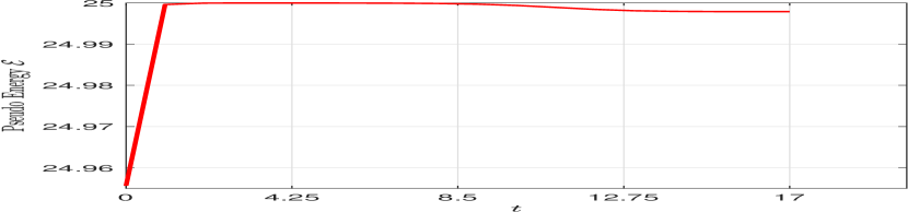
(a) Backward-Euler scheme

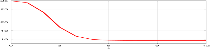
(b) First-order Convex-splitting scheme

Figure 1: Pseudo-energy decay comparison: Backward Euler scheme (B.3)-(B.4) vs. First-order Convex-splitting scheme (3.1)-(3.2) for $\tau=1$ in Example 4.2.

In the following two examples of this subsection, we compare the numerical efficiency of the proposed second-order flow methods with those of the gradient flow methods. The gradient flow and its corresponding convex-splitting schemes are provided in B.2.

Example 4.3.

We consider a computational domain of $[0,2\pi]\times[0,2\pi]$ with an initial value $u_{0}(x,y)=tanh(x-2y)\cdot sin(x)\cdot cos(x)$. Notably, this initial value is distinct from the ground state. We select a parameter value of $\epsilon=0.05$ and adhere to the previously mentioned stopping criteria (4.1)-(4.2), where both $\varepsilon_{r}$ and $\varepsilon_{v}$ are fixed at $10^{-3}$. Four distinct computational strategies are employed in this experiment: the first-order and second-order convex-splitting schemes for gradient flow (GF-CS-1st and GF-CS-2nd, respectively) and for second-order flow (SF-CS-1st and SF-CS-2nd, respectively). The time step size is chosen to be $\tau=0.1$ for second-order schemes and $\tau=0.01$ for first-order schemes, with a spatial grid size of $h=1/128$.

As depicted in Figure 2, we implement the first-order and second-order convex-splitting schemes to the gradient and second-order flows, respectively, and assess their impact on the rate of energy decay. It was observed that the second-order flow methods exhibits certain advantage over the gradient flow methods in terms of energy decay rate, although gradient flow methods have already been quite efficient in this scenario.

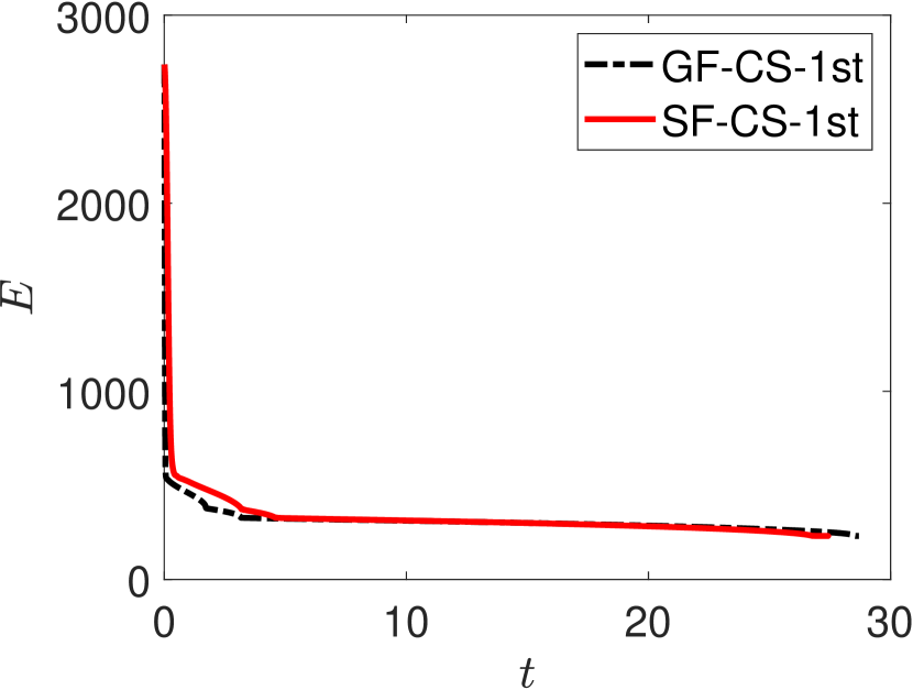
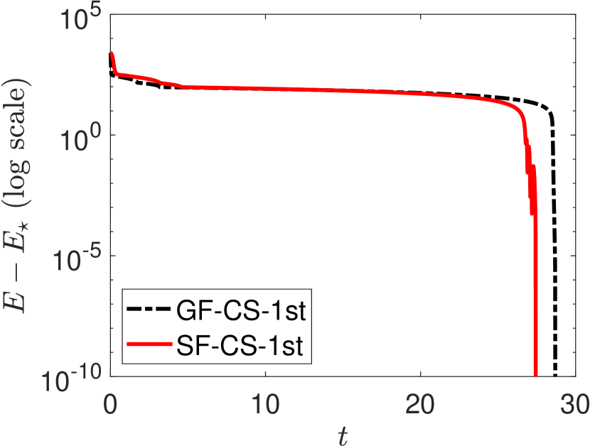
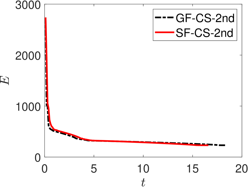
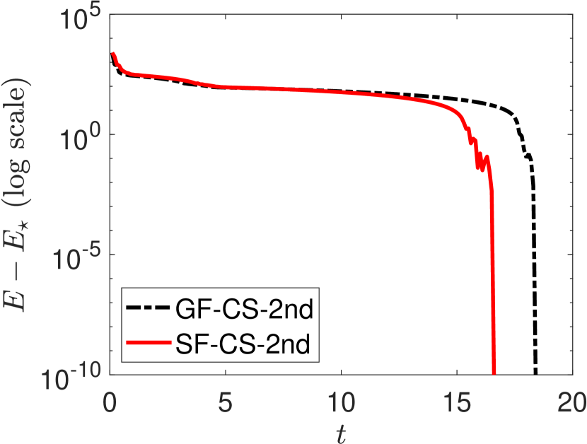
Figure 2: Comparison of energy evolution (left column) and energy level convergence (right column) over iterations for Example 4.3 (an isotropic case) using Gradient Flow (GF-CS-1st $\&$ GF-CS-2nd) and Second-order Flow (SF-CS-1st $\&$ SF-CS-2nd) methodologies. Within the figures, $E$ denotes the calculated energy, while $E_{\star}$ signifies the minimum energy achieved throughout the iterations.

Example 4.4.

We consider an anisotropic variant of the original Ginzburg-Landau energy (4.3). The anisotropic energy functional, $E_{aniso}(u)$, is defined by:

$$E_{aniso}(u)=\int_{\Omega}\left(\frac{1}{2}\left(k_{x}(\partial_{x}u)^{2}+k_{y}(\partial_{y}u)^{2}\right)+\frac{1}{4\epsilon^{2}}(u^{2}-1)^{2}\right)dx.$$ (4.5)

In this formulation, we set $k_{x}=\frac{1}{100}$ and $k_{y}=1$ to have a clear anisotropy. All other parameters are aligned with those used in Example 4.3. The experiment compare the rate of energy decay between the Gradient Flow and Second-order Flow. Given the lower computational efficiency and higher computational cost of the first-order schemes observed in example 4.3, in this more complex scenario, we only compared the results of the second-order schemes and did not evaluate the first-order schemes.

As depicted in Figure 3, the trajectories clearly indicate the superior performance of a second-order flow method over its gradient flow counterpart. The energy reduction pace is notably faster than the gradient flow method, underlining the enhanced efficiency of the second-order flow, especially in an anisotropic context.

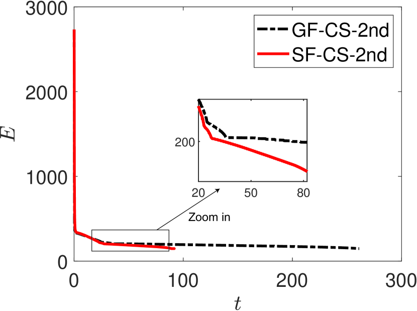
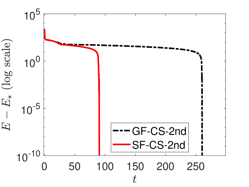
Figure 3: Comparison of energy evolution (left column) and energy discrepancy (right column) over iterations for Example 4.4 (an anisotropic case) using Gradient Flow (GF-CS-2nd) and Second-order Flow (SF-CS-2nd) methodologies.

Remark 4.1.

This anisotropic term reduces the uniform convexity of the quadratic term in the energy functional, which makes gradient flow methods not so efficient as in the isotropic case. This example highlights the advantages of the second-order flows, which accelerate the minimization algorithm when the convexity of the energy functional is challenged. Notice that the theoretical results established in this paper are also valid for the anisotropic form energy functional.

4.2 Landau–de Gennes (LdG) model

The LdG model is widely recognized for its role in characterizing liquid crystal ordering, treating the free energy as a functional of the $\mathbf{Q}$-tensor field, as detailed in various studies [10, 30, 51, 54]. For two-dimensional nematic liquid crystals, the LdG free energy functional is delineated as follows [54]:

$$J(\mathbf{Q})=\int\left\{\frac{1}{2}|\nabla\mathbf{Q}|^{2}+\vartheta F(\mathbf{Q})\right\}\,\mathrm{d}\mathbf{r},$$

where $\vartheta$ is a positive parameter, and the one-constant approximation [5] has been assumed, leading to the isotropic term $|\nabla\mathbf{Q}|^{2}$. The $\mathbf{Q}$-tensor at a point $\mathbf{r}=(x,y)$ represents the orientational order of the liquid crystals and is characterized by a $2\times 2$ traceless and symmetric matrix:

$$\mathbf{Q}=\begin{pmatrix}p_{1}&p_{2}\\ p_{2}&-p_{1}\end{pmatrix}.$$

The square of the Frobenius norm of $\nabla\mathbf{Q}$ is computed as $|\nabla\mathbf{Q}|^{2}=2\left(|\nabla p_{1}|^{2}+|\nabla p_{2}|^{2}\right)$. The bulk free energy, or Landau function $F(\mathbf{Q})$, is most often taken to be of the general form [36]:

$$F(\mathbf{Q})=\frac{a}{4}\operatorname{tr}\left(\mathbf{Q}^{2}\right)-\frac{b}{6}\operatorname{tr}\left(\mathbf{Q}^{3}\right)+\frac{c}{8}\left(\operatorname{tr}\left(\mathbf{Q}^{2}\right)\right)^{2},$$

in which $a$ signifies the reduced temperature difference, $b\geq 0$ and $c>0$. For our experiments, we consider the particular case

$$F(\mathbf{Q})=\frac{a}{4}\operatorname{tr}\left(\mathbf{Q}^{2}\right)+\frac{1}{8}\left(\operatorname{tr}\left(\mathbf{Q}^{2}\right)\right)^{2}=\frac{a}{2}(|p_{1}|^{2}+|p_{2}|^{2})+\frac{1}{2}(|p_{1}|^{2}+|p_{2}|^{2})^{2}.$$

We then introduce $\mathbf{u}=\begin{bmatrix}p_{1}\\ p_{2}\end{bmatrix}$, with the magnitude $|\mathbf{u}|=\sqrt{|p_{1}|^{2}+|p_{2}|^{2}}$. Consequently, the energy functional in terms of $\mathbf{u}$ is expressed as:

$$E(\mathbf{u}) =\int_{\Omega}\left\{|\nabla\mathbf{u}|^{2}+\vartheta\left(\frac{a}{2}|\mathbf{u}|^{2}+\frac{1}{2}|\mathbf{u}|^{4}\right)\right\}\mathrm{d}\mathbf{r}.$$ (4.6)

It follows that $J(\mathbf{Q})$ is equivalent to $E(\mathbf{u})$. The objective is to find stable liquid crystal configurations by minimizing the energy functional $E(\mathbf{u})$, subject to certain boundary conditions. This problem formulation aligns with the energy minimization problem described in Equation (1.1). After a steady state solution is found, the generally nonuniform, undiagonalized $\mathbf{Q}(\mathbf{r})$ can be analyzed by computing its eigenvalues,

$$S(\mathbf{r})/2=\pm\sqrt{p_{1}(\mathbf{r})^{2}+p_{2}(\mathbf{r})^{2}}.$$

A nematic region has $|S(\mathbf{r})|/S_{0}=1$ and isotropic state $|S(\mathbf{r})|/S_{0}=0$. The nematic field director is given by the eigenvector of $\mathbf{Q}(\mathbf{r})$ (for example, corresponding to the positive eigenvalue),

$$\mathbf{n}(\mathbf{r})=\left(\sqrt{1/2+p_{1}(\mathbf{r})/|S(\mathbf{r})|},\sigma(\mathbf{r})\sqrt{1/2-p_{1}(\mathbf{r})/|S(\mathbf{r})|}\right),$$

with $\sigma(\mathbf{r})=\mathbf{1}_{\left\{p_{2}\geq 0\right\}}(\mathbf{r})-\mathbf{1}_{\left\{p_{2}<0\right\}}(\mathbf{r})$ and $\mathbf{1}$ the indicator function.

Example 4.5.

To ensure the system in the nematic phase, we select a low temperature setting with $a=-1.672$. The domain $\Omega=[-1,1]\times[-1,1]$ is selected for square confinement. For the Dirichlet boundary conditions, we impose

$$\mathbf{u}(x,y=\pm 1)=\frac{\sqrt{2|a|}}{2}\begin{pmatrix}1&0\\ 0&-1\end{pmatrix},\quad\mathbf{u}(x=\pm 1,y)=\frac{\sqrt{2|a|}}{2}\begin{pmatrix}-1&0\\ 0&1\end{pmatrix}.$$

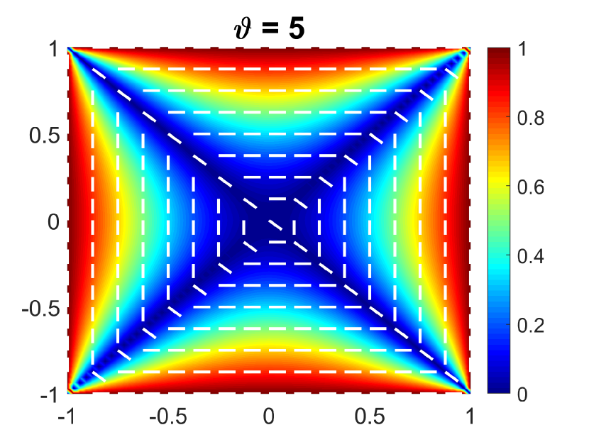
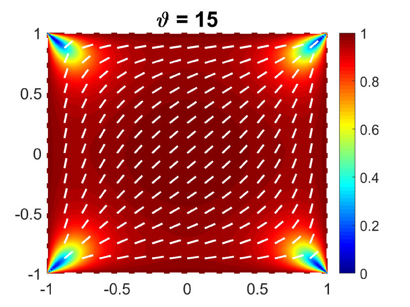
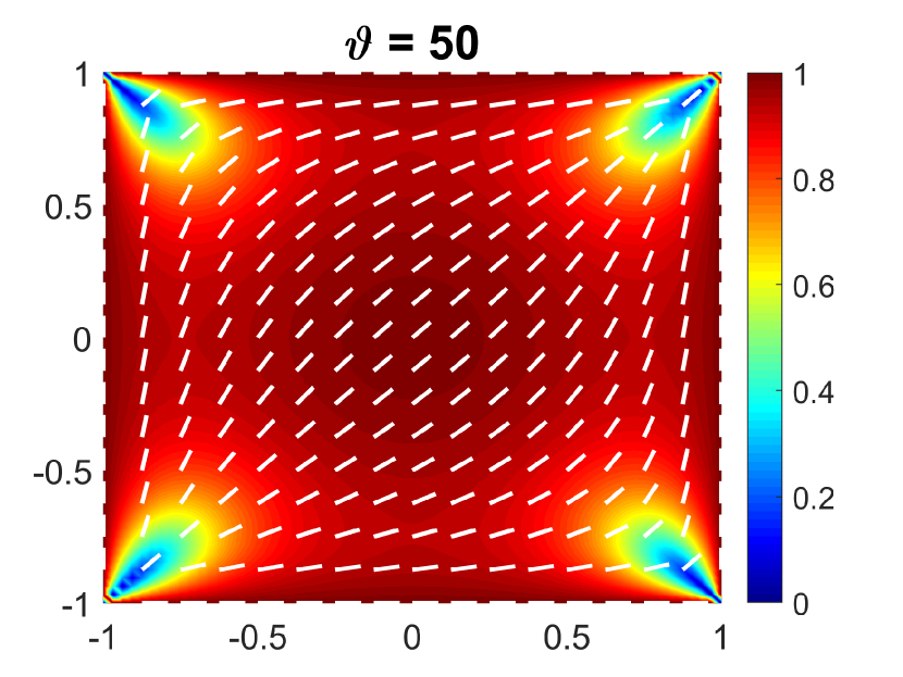
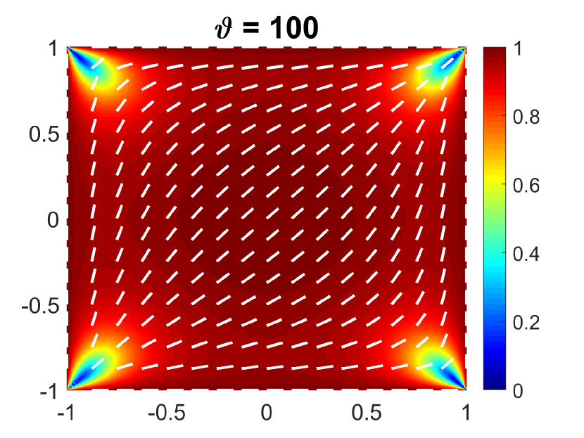
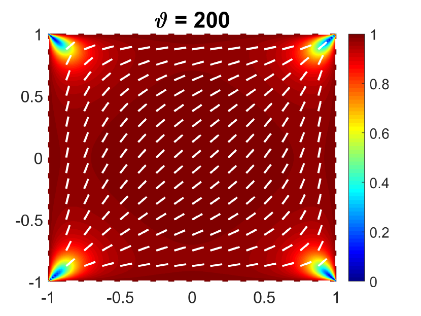
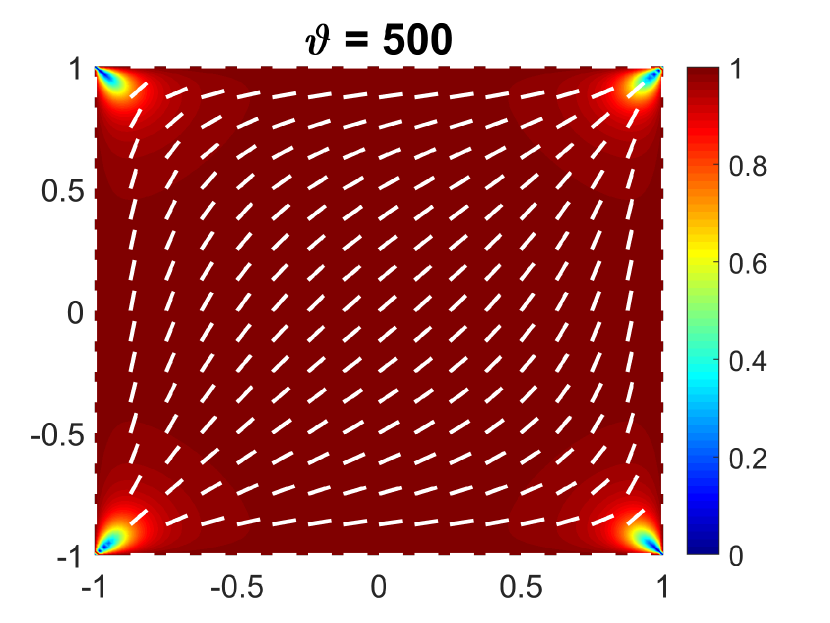
Figure 4: Stable liquid crystal configurations at varying $\vartheta$ values (5, 15, 50, 100, 200, 500), computed via the second-order flow method. The color gradient indicates the relative intensity of directional ordering, quantified as $|S(\mathbf{r})|/S_{0}$. The white bars depict the directional vectors of the nematic field, $\mathbf{n}(\mathbf{r})$.

The chosen boundary conditions for the Q-tensor, aligning the nematic director parallel to the square boundary lines, represents a common approach in the modeling of liquid crystals confined within geometries [14]. To compute the stationary points of the LdG free energy, the second-order flow method is applied, utilizing the scheme outlined in equations (3.3) to (3.4). We select a time step size of $\tau=0.1$, initiate our simulations with random initial conditions, and specify the tolerances for the stopping criteria in (4.1)-(4.2) as $\varepsilon_{r}=10^{-10}$ and $\varepsilon_{v}=10^{-10}$. The results depict stable liquid crystal configurations for varying values of $\vartheta$. Specifically, for $\vartheta$ values of 5, 15, and 50, we use a grid size of $h=1/64$, while for $\vartheta$ values of 100, 200, and 500, we opt for a finer grid size of $h=1/128$. The computed configurations are presented in Figure 4.

5 Conclusion

In this paper, we have strived to develop numerical analysis for the recently proposed computational framework of second-order flows for non-convex variational problems. As an initial step in this direction, we have established a convergence analysis of numerical discretizations via convex-splitting schemes, which we have used to define two different numerical schemes, with first and second order timestepping respectively. Starting with semi-discrete formulations, we have proved their subsequential convergence to a stationary point of the original non-convex energy and, by making the timestep vanish, used them to establish well-posedness of the ensuing second-order flows. On the fully discrete level, we have proved convergence and error estimates with the expected rates for both numerical schemes.

Through several illustrative numerical examples, we have verified the accuracy and convergence of both schemes. Notably, the two schemes exhibit unconditional pseudo-energy stability and unconditional unique solvability simultaneously, highlighting their advantages over other numerical schemes. Furthermore, we have again witnessed that second-order flows, as the minimization strategy for non-convex variational problems, show their efficiency especially notable when dealing with functional of increased complexity and non-convexity. Their versatility has also been affirmed through the application to the tensor-valued Landau–de Gennes model.

This investigation, however, is not conclusive; it rather paves the way to deepen our exploration along this direction. Interesting aspects from the optimization point of view, like the convergence of complete trajectories and associated convergence rates to stationary points, are on the agenda of our next steps.

Acknowledgements

The work of H. Chen and G. Dong was supported by NSFC grant 12001194. The work of W. Liu was partially supported by the Ministry of Education of Singapore under its AcRF Tier 2 funding MOE-T2EP20122-0002 (A-8000962-00-00) and partially supported by NSFC grant 12101252 and the Guangdong Basic and Applied Basic Research Foundation grant 2022A1515010351 through South China Normal University. The work of H. Chen and Z. Xie was supported by NSFC grant 12171148. The authors acknowledge some helpful discussions with Prof. Chen Wang on the error analysis of the numerical schemes.

Appendix A Error estimates of quantities for the second-order scheme

Lemma A.1.

Suppose that $\mathbf{u}$ is the real solution of (1.6), with regularities (3.5) and (3.7). Then, for all $h,\tau>0$, there exists $C>0$, independent of $h$ and $\tau$, such that for $0\leq k\leq\ell-1$

$$\left\|\sigma_{1}^{k+\frac{1}{2}}\right\|_{L^{2}}^{2}\leq C\frac{h^{2q+2}}{\tau}\int_{t_{k}}^{t_{k+1}}\left\|\partial_{s}\mathbf{u}(s)\right\|_{H^{q+1}}^{2}ds,$$ (A.1)

$$\left\|\sigma_{2}^{k+\frac{1}{2}}\right\|_{L^{2}}^{2}\leq C\tau^{3}\int_{t_{k}}^{t_{k+1}}\left\|\partial_{s}^{3}\mathbf{u}(s)\right\|_{L^{2}}^{2}ds,$$ (A.2)

$$\left\|\varsigma_{1}^{k+\frac{1}{2}}\right\|_{L^{2}}^{2}\leq C\frac{h^{2q+2}}{\tau}\int_{t_{k}}^{t_{k+1}}\left\|\partial_{s}^{2}\mathbf{u}(s)\right\|_{H^{q+1}}^{2}ds+C\tau^{3}\int_{t_{k}}^{t_{k+1}}\left\|\partial_{s}^{4}\mathbf{u}(s)\right\|_{L^{2}}^{2}ds,$$ (A.3)

$$\left\|\varsigma_{2}^{k+\frac{1}{2}}\right\|_{L^{2}}^{2}\leq C\tau^{3}\int_{t_{k}}^{t_{k+1}}\left\|\partial_{s}^{4}\mathbf{u}(s)\right\|_{L^{2}}^{2}ds,$$ (A.4)

$$\left\|\varsigma_{3}^{k+\frac{1}{2}}\right\|_{L^{2}}^{2}\leq C\tau^{5}\int_{t_{k}}^{t_{k+1}}\left\|\partial_{s}^{4}\mathbf{u}(s)\right\|_{L^{2}}^{2}ds,$$ (A.5)

$$\left\|\frac{1}{2}\mathbf{u}^{k+1}+\frac{1}{2}\mathbf{u}^{k}-\mathbf{u}^{k+\frac{1}{2}}\right\|_{L^{2}}^{2}\leq C\tau^{3}\int_{t_{k}}^{t_{k+1}}\left\|\partial_{s}^{2}\mathbf{u}(s)\right\|_{L^{2}}^{2}ds,$$ (A.6)

$$\left\|\Delta\sigma_{3}^{k+\frac{1}{2}}\right\|_{L^{2}}^{2}\leq C\tau^{3}\int_{t_{k}}^{t_{k+1}}\left\|\partial_{s}^{2}\Delta\mathbf{u}(s)\right\|_{L^{2}}^{2}ds,$$ (A.7)

$$\left\|\frac{1}{2}(\mathbf{u}^{k+1})^{2}+\frac{1}{2}(\mathbf{u}^{k})^{2}-(\mathbf{u}^{k+\frac{1}{2}})^{2}\right\|_{L^{2}}^{2}\leq C\tau^{3}\int_{t_{k}}^{t_{k+1}}\left\|\partial_{s}^{2}\mathbf{u}^{2}(s)\right\|_{L^{2}}^{2}ds,$$ (A.8)

and for $1\leq k\leq\ell-1$

$$\left\|\mathbf{u}^{k+\frac{1}{2}}-\frac{3}{2}\mathbf{u}^{k}-\frac{1}{2}\mathbf{u}^{k-1}\right\|_{L^{2}}^{2}\leq C\tau^{3}\int_{t_{k-1}}^{t_{k+1}}\left\|\partial_{s}^{2}\mathbf{u}(s)\right\|_{L^{2}}^{2}\mathrm{~{}d}s.$$ (A.9)

Proof.

The proof of each of the inequalities above is a direct application of Taylor’s theorem with integral remainder. We suppress the details for the sake of brevity. ∎

Lemma A.2.

Suppose that $\mathbf{u}$ is the real solution of (1.6), with regularities (3.5) and (3.7). Then, for all $h,\tau>0$, there exists $C>0$, independent of $h$ and $\tau$, such that for $0\leq k\leq\ell-1$

$$\left\|\sigma_{4}^{k+\frac{1}{2}}\right\|_{L^{2}}^{2}\leq C\tau^{3}\int_{t_{k}}^{t_{k+1}}\left\|\partial_{s}^{2}\mathbf{u}(s)\right\|_{L^{2}}^{2}+\left\|\partial_{s}^{2}\mathbf{u}^{2}(s)\right\|_{L^{2}}^{2}ds,$$ (A.10)

$$\left\|\sigma_{5}^{k+\frac{1}{2}}\right\|_{L^{2}}^{2}\leq C\left(\left\|\mathcal{D}^{\mathbf{u},k+1}\right\|_{L^{2}}^{2}+\left\|\mathcal{D}^{\mathbf{u},k}\right\|_{L^{2}}^{2}\right),$$ (A.11)

$$\left\|\sigma_{6}^{k+\frac{1}{2}}\right\|_{L^{2}}^{2}\leq (1-\delta_{0,k})C\tau^{3}\int_{t_{k-1}}^{t_{k}}\left\|\partial_{s}^{2}\mathbf{u}(s)\right\|_{L^{2}}^{2}ds+C\tau^{3}\int_{t_{k}}^{t_{k+1}}\left\|\partial_{s}^{2}\mathbf{u}(s)\right\|_{L^{2}}^{2}ds$$

$$+C\left\|\mathcal{D}^{\mathbf{u},k}\right\|_{L^{2}}^{2}+(1-\delta_{0,k})C\left\|\mathcal{D}^{\mathbf{u},k-1}\right\|_{L^{2}}^{2},$$ (A.12)

where $\delta_{n,m}$ is the Kronecker delta.

Proof.

Proof of estimate (A.10).

By utilizing the triangle inequality and Young’s inequality, we obtain

$$\left\|\sigma_{4}^{k+\frac{1}{2}}\right\|_{L^{2}}\leq\left\|\frac{(\mathbf{u}^{k+1})^{2}+(\mathbf{u}^{k})^{2}}{2}\left(\frac{\mathbf{u}^{k+1}+\mathbf{u}^{k}}{2}-\mathbf{u}^{k+\frac{1}{2}}\right)\right.+\left.\mathbf{u}^{k+\frac{1}{2}}\left(\frac{(\mathbf{u}^{k+1})^{2}+(\mathbf{u}^{k})^{2}}{2}-(\mathbf{u}^{k+\frac{1}{2}})^{2}\right)\right\|_{L^{2}}$$

$$\leq \frac{1}{2}\left\|(\mathbf{u}^{k+1})^{2}+(\mathbf{u}^{k})^{2}\right\|_{L^{\infty}}\left\|\frac{1}{2}\mathbf{u}^{k+1}+\frac{1}{2}\mathbf{u}^{k}-\mathbf{u}^{k+\frac{1}{2}}\right\|_{L^{2}}+\left\|\mathbf{u}^{k+\frac{1}{2}}\right\|_{L^{\infty}}\left\|\frac{1}{2}(\mathbf{u}^{k+1})^{2}+\frac{1}{2}(\mathbf{u}^{k})^{2}-(\mathbf{u}^{k+\frac{1}{2}})^{2}\right\|_{L^{2}}.$$

Using the assumed regularities (3.5) and (3.7) of the PDE solution, and invoking the truncation error estimates (A.6) and (A.8), the result follows.

Proof of estimate (A.11).

We commence by expanding the expression in detail as follows:

$$4\sigma_{5}^{k+\frac{1}{2}}= 4\chi\left(\mathbf{u}_{h}^{k+1},\mathbf{u}_{h}^{k}\right)-4\chi\left(\mathbf{u}^{k+1},\mathbf{u}^{k}\right)$$

$$= \left\{\left(\mathbf{u}_{h}^{k+1}\right)^{2}+\left(\mathbf{u}_{h}^{k}\right)^{2}+\left(\mathbf{u}_{h}^{k+1}+\mathbf{u}^{k+1}\right)\left(\mathbf{u}^{k+1}+\mathbf{u}^{k}\right)\right\}\left(\mathbf{u}_{h}^{k+1}-\mathbf{u}^{k+1}\right)$$

$$+\left\{\left(\mathbf{u}_{h}^{k+1}\right)^{2}+\left(\mathbf{u}_{h}^{k}\right)^{2}+\left(\mathbf{u}_{h}^{k}+\mathbf{u}^{k}\right)\left(\mathbf{u}^{k+1}+\mathbf{u}^{k}\right)\right\}\left(\mathbf{u}_{h}^{k}-\mathbf{u}^{k}\right).$$

Next, invoking the assumed regularities (3.7) of the PDE solution, and utilizing the properties of $f$, we obtain, for $k=0,1,\ldots,\ell$,,

$$\left\|\sigma_{5}^{k+\frac{1}{2}}\right\|_{L^{2}}\leq C\left\|1+(\mathbf{u}_{h}^{k})^{2}+(\mathbf{u}^{k})^{2}+(\mathbf{u}_{h}^{k+1})^{2}+(\mathbf{u}^{k+1})^{2}\right\|_{L^{\infty}}\left(\left\|\mathcal{D}^{\mathbf{u},k+1}\right\|_{L^{2}}+\left\|\mathcal{D}^{\mathbf{u},k}\right\|_{L^{2}}\right).$$

Proof of estimate (A.12).

For $k=0$, we have

$$\left\|\sigma_{6}^{1/2}\right\|_{L^{2}}^{2}\leq\left\|\left(\mathbf{u}^{\frac{1}{2}}-\mathbf{u}_{0}-\frac{\tau}{2}\partial_{t}\mathbf{u}(0)\right)\right\|_{L^{2}}^{2}+\left\|\left(\mathbf{u}_{0}-\mathbf{u}_{h}^{0}\right)\right\|_{L^{2}}^{2}\leq C\tau^{3}\int_{t_{0}}^{t_{\frac{1}{2}}}\left\|\partial_{s}^{2}\mathbf{u}(s)\right\|_{L^{2}}^{2}\mathrm{~{}d}s+C\left\|\mathcal{D}^{\mathbf{u},0}\right\|_{L^{2}}^{2}.$$

For $0\leqslant k\leqslant\ell-1$, using the truncation error (A.9), we obtain

$$\left\|\sigma_{6}^{k+\frac{1}{2}}\right\|_{L^{2}}^{2}\leq C\tau^{3}\int_{t_{k-1}}^{t_{k+1}}\left\|\partial_{s}^{2}\mathbf{u}(s)\right\|_{L^{2}}^{2}\mathrm{~{}d}s+C\left\|\mathcal{E}^{\mathbf{u},k}\right\|_{L^{2}}^{2}+C\left\|\mathcal{E}^{\mathbf{u},k-1}\right\|_{L^{2}}^{2}.$$

∎

Appendix B Other numerical methods

B.1 Additional numerical schemes for second-order flow

Forward Euler Scheme

$$(\mathbf{v}_{h}^{k+1}-\mathbf{v}_{h}^{k},\xi)+\tau\eta^{k}(\mathbf{v}_{h}^{k},\xi)+\tau\left(a(\mathbf{u}_{h}^{k},\xi)+(f(\mathbf{u}_{h}^{k}),\xi)\right)=0,\quad\forall\xi\in S_{h},$$ (B.1)

$$(\mathbf{u}_{h}^{k+1}-\mathbf{u}_{h}^{k},\zeta)-\tau(\mathbf{v}_{h}^{k+1},\zeta)=0,\quad\forall\zeta\in S_{h},$$ (B.2)

with initial conditions $\mathbf{u}_{h}^{0}=R_{h}\mathbf{u}_{0}$ and $\mathbf{v}_{h}^{0}\equiv\mathbf{0}$.

Backward Euler Scheme

$$(\mathbf{v}_{h}^{k+1}-\mathbf{v}_{h}^{k},\xi)+\tau\eta^{k+1}(\mathbf{v}_{h}^{k+1},\xi)+\tau\left(a(\mathbf{u}_{h}^{k+1},\xi)+(f(\mathbf{u}_{h}^{k+1}),\xi)\right)=0,\quad\forall\xi\in S_{h},$$ (B.3)

$$(\mathbf{u}_{h}^{k+1}-\mathbf{u}_{h}^{k},\zeta)-\tau(\mathbf{v}_{h}^{k+1},\zeta)=0,\quad\forall\zeta\in S_{h},$$ (B.4)

with initial conditions $\mathbf{u}_{h}^{0}=R_{h}\mathbf{u}_{0}$ and $\mathbf{v}_{h}^{0}\equiv\mathbf{0}$.

Semi-implicit Scheme

$$(\mathbf{u}_{h}^{k+1}-2\mathbf{u}_{h}^{k}+\mathbf{u}_{h}^{k-1},\xi) +\frac{\tau\eta^{k+\frac{1}{2}}}{2}(\mathbf{u}_{h}^{k+1}-\mathbf{u}_{h}^{k-1},\xi)$$

$$+\tau^{2}\left(a\left(\frac{\mathbf{u}_{h}^{k+1}+\mathbf{u}_{h}^{k-1}}{2},\xi\right)+(f(\mathbf{u}_{h}^{k}),\xi)\right)=0,\quad\forall\xi\in S_{h},$$ (B.5)

with the initial conditions $\mathbf{u}_{h}^{0}=R_{h}\mathbf{u}_{0}$ and $\mathbf{v}_{h}^{0}\equiv\mathbf{0}$. For the first step, the scheme is given by

$$(\mathbf{u}_{h}^{1},\xi)=(\mathbf{u}_{h}^{0},\xi)-\frac{\tau^{2}}{2}\left(a(\mathbf{u}_{h}^{0},\xi)+(f(\mathbf{u}_{h}^{0}),\xi)\right),\quad\forall\xi\in S_{h}.$$ (B.6)

Crank-Nicolson Scheme

$$(\mathbf{v}_{h}^{k+1}-\mathbf{v}_{h}^{k},\xi)+\tau\eta^{k+\frac{1}{2}}(\mathbf{v}_{h}^{k+\frac{1}{2}},\xi)$$

$$\qquad+\tau\left(a(\mathbf{u}_{h}^{k+\frac{1}{2}},\xi)+\left(\frac{F(\mathbf{u}_{h}^{k+1})-F(\mathbf{u}_{h}^{k})}{\mathbf{u}_{h}^{k+1}-\mathbf{u}_{h}^{k}},\xi\right)\right)=0,\quad\forall\xi\in S_{h},$$ (B.7)

$$(\mathbf{u}_{h}^{k+1}-\mathbf{u}_{h}^{k},\zeta)-\tau(\mathbf{v}_{h}^{k+\frac{1}{2}},\zeta)=0,\quad\forall\zeta\in S_{h},$$ (B.8)

with initial conditions $\mathbf{u}_{h}^{-1}=\mathbf{u}_{h}^{0}=R_{h}\mathbf{u}_{0}$ and $\mathbf{v}_{h}^{0}\equiv\mathbf{0}$.

B.2 Gradient flow and its convex-splitting schemes

In this section, we describe gradient flow methods for computing the ground state solution defined in (1.1).

$$\begin{cases}\partial_{t}{\mathbf{u}}=\Delta\mathbf{u}-f(\mathbf{u}),&\text{ in }[0,T]\times\Omega,\\ \mathbf{u}(0)=\mathbf{u}_{0},&\text{ in }\Omega,\\ \mathbf{u}=0,&\text{ on }[0,T]\times\partial\Omega\end{cases}.$$ (B.9)

Likewise, for the gradient flow (B.9), we introduce a first-order and a second-order fully discrete convex-splitting scheme respectively as follows:

First-order Convex-splitting scheme for Gradient Flow

Given $\mathbf{u}_{h}^{k},\mathbf{v}_{h}^{k}\in S_{h}$, find $\mathbf{u}_{h}^{k+1},\mathbf{v}_{h}^{k+1}\in S_{h}$ such that:

$$(\mathbf{u}_{h}^{k+1}-\mathbf{u}_{h}^{k},\xi)+\tau\left(a(\mathbf{u}_{h}^{k+1},\xi)+(f_{c}(\mathbf{u}_{h}^{k+1})-f_{e}(\mathbf{u}_{h}^{k}),\xi)\right)=0\quad\forall\xi\in S_{h},$$ (B.10)

Here, $\tau>0$ is the time step size, and the initial conditions are given by $\mathbf{u}_{h}^{0}=R_{h}\mathbf{u}_{0}$.

Second-order Convex-splitting scheme for Gradient Flow

Given $\mathbf{u}_{h}^{k},\mathbf{v}_{h}^{k}\in S_{h}$, find $\mathbf{u}_{h}^{k+1},\mathbf{v}_{h}^{k+1}\in S_{h}$ such that:

$$(\mathbf{u}_{h}^{k+1}-\mathbf{u}_{h}^{k},\xi)+\tau\left(a(\mathbf{u}_{h}^{k+\frac{1}{2}},\xi)+\left(\chi(\mathbf{u}_{h}^{k+1},\mathbf{u}_{h}^{k})-f_{e}(\widetilde{\mathbf{u}}_{h}^{k-\frac{1}{2}}),\xi\right)\right)=0\quad\forall\xi\in S_{h},$$ (B.11)

where

$$\chi\left(\phi,\psi\right)=\int_{0}^{1}f_{c}(\theta\phi+(1-\theta)\psi)d\theta=\frac{F_{c}(\phi)-F_{c}(\psi)}{\phi-\psi}\quad\text{and}\quad\widetilde{\mathbf{u}}_{h}^{k-\frac{1}{2}}=\frac{3}{2}\mathbf{u}_{h}^{k}-\frac{1}{2}\mathbf{u}_{h}^{k-1}.$$

The initial condition is setting as $\mathbf{u}_{h}^{-1}=\mathbf{u}_{h}^{0}=R_{h}\mathbf{u}_{0}$.

References

- [1] R. A. Adams and J. J. F. Fournier. Sobolev spaces, volume 140 of Pure and Applied Mathematics (Amsterdam). Elsevier/Academic Press, Amsterdam, second edition, 2003.
- [2] D. M. Anderson, G. B. McFadden, and A. A. Wheeler. Diffuse-interface methods in fluid mechanics. Annu. Rev. Fluid Mech., 30(1):139–165, 1998.
- [3] H. Attouch, R. Boţ, and E. Csetnek. Fast optimization via inertial dynamics with closed-loop damping. J. Eur. Math. Soc., 25(5):1985–2056, 2023.
- [4] H. Attouch, Z. Chbani, J. Peypouquet, and P. Redont. Fast convergence of inertial dynamics and algorithms with asymptotic vanishing viscosity. Math. Program., 168(1):123–175, 2018.
- [5] J. M. Ball. Mathematics and liquid crystals. Mol. Cryst. Liq. Cryst., 647(1):1–27, 2017.
- [6] A. Baskaran, Z. Hu, J. S. Lowengrub, C. Wang, S. M. Wise, and P. Zhou. Energy stable and efficient finite-difference nonlinear multigrid schemes for the modified phase field crystal equation. J. Comput. Phys., 250:270–292, 2013.
- [7] A. Baskaran, J. S. Lowengrub, C. Wang, and S. M. Wise. Convergence analysis of a second order convex splitting scheme for the modified phase field crystal equation. SIAM J. Numer. Anal., 51(5):2851–2873, 2013.
- [8] P. Bégout, J. Bolte, and M. A. Jendoubi. On damped second-order gradient systems. J. Differential Equations, 259(7):3115–3143, 2015.
- [9] R. Boţ, G. Dong, P. Elbau, and O. Scherzer. Convergence rates of first- and higher-order dynamics for solving linear ill-posed problems. Found. Comput. Math., 22:1567–1629, 2022.
- [10] Y. Cai, J. Shen, and X. Xu. A stable scheme and its convergence analysis for a 2D dynamic -tensor model of nematic liquid crystals. Math. Models Methods Appl. Sci., 27(08):1459–1488, 2017.
- [11] H. Chen, G. Dong, W. Liu, and Z. Xie. Second-order flows for computing the ground states of rotating Bose-Einstein condensates. J. Comput. Phys., 475:111872, 2023.
- [12] L.-Q. Chen. Phase-field models for microstructure evolution. Annu. Rev. Mater. Res., 32(1):113–140, 2002.
- [13] L. Q. Chen and J. Shen. Applications of semi-implicit Fourier-spectral method to phase field equations. Comput. Phys. Commun., 108:147–158, 1998.
- [14] P. de Gennes and J. Prost. The Physics of Liquid Crystals. Oxford University Press, Oxford, UK, 2 edition, 1993.
- [15] A. E. Diegel, X. H. Feng, and S. M. Wise. Analysis of a mixed finite element method for a Cahn–Hilliard–Darcy–Stokes system. SIAM J. Numer. Anal., 53(1):127–152, 2015.
- [16] G. Dong, M. Hintermueller, and Y. Zhang. A class of second-order geometric quasilinear hyperbolic PDEs and their application in imaging. SIAM J. Imaging Sci., 14(2):645–688, 2021.
- [17] S. S. Dragomir. Some Gronwall type inequalities and applications. Nova Science Publishers, Inc., Hauppauge, NY, 2003.
- [18] Q. Du, C. Liu, and X. Wang. A phase field approach in the numerical study of the elastic bending energy for vesicle membranes. J. Comput. Phys., 198(2):450–468, 2004.
- [19] Q. Du, C. Liu, and X. Wang. Simulating the deformation of vesicle membranes under elastic bending energy in three dimensions. J. Comput. Phys., 212(2):757–777, 2006.
- [20] S. Edvardsson, M. Gulliksson, and J. Persson. The dynamical functional particle method: An approach for boundary value problems. J. Appl. Mech., 79(2):021012, 2012.
- [21] L. C. Evans. Partial Differential Equations, volume 19 of Graduate Studies in Mathematics. American Mathematical Society, second edition, 2010.
- [22] D. J. Eyre. Unconditionally gradient stable time marching the Cahn-Hilliard equation. In J. W. Bullard, R. Kalia, M. Stoneham, and L. Q. Chen, editors, Computational and Mathematical Models of Microstructural Evolution, volume 529 of Mater. Res. Soc. Symp. Proc., pages 39–46. Cambridge University Press, 1998.
- [23] X. Feng and S. Wise. Analysis of a Darcy–Cahn–Hilliard diffuse interface model for the hele-shaw flow and its fully discrete finite element approximation. SIAM J. Numer. Anal., 50(3):1320–1343, 2012.
- [24] P. Galenko. Phase-field model with relaxation of the diffusion flux in nonequilibrium solidification of a binary system. Phys. Lett. A, 287:190–197, 2001.
- [25] P. Galenko and D. Jou. Diffuse-interface model for rapid phase transformations in nonequilibrium systems. Phys. Rev. E, 71(4):046125, 2005.
- [26] P. Grisvard. Elliptic problems in nonsmooth domains, volume 24 of Monographs and Studies in Mathematics. Pitman (Advanced Publishing Program), Boston, MA, 1985.
- [27] A. Haraux and M. A. Jendoubi. Convergence of bounded weak solutions of the wave equation with dissipation and analytic nonlinearity. Calc. Var. Partial Differential Equations, 9(2):95–124, 1999.
- [28] J. G. Heywood and R. Rannacher. Finite element approximation of the nonstationary Navier–Stokes problem. I. Regularity of solutions and second-order error estimates for spatial discretization. SIAM J. Numer. Anal., 19(2):275–311, 1982.
- [29] Z. Hu, S. M. Wise, C. Wang, and J. S. Lowengrub. Stable and efficient finite-difference nonlinear-multigrid schemes for the phase field crystal equation. J. Comput. Phys., 228(15):5323–5339, 2009.
- [30] T. Huang and N. Zhao. On the regularity of weak small solution of a gradient flow of the Landau–de Gennes energy. Proc. Amer. Math. Soc., 147(4):1687–1698, 2019.
- [31] G. Iyer, X. Xu, and A. D. Zarnescu. Dynamic cubic instability in a 2D Q-tensor model for liquid crystals. Math. Models Methods Appl. Sci., 25(08):1477–1517, 2015.
- [32] J. Kačur. Application of Rothe’s method to perturbed linear hyperbolic equations and variational inequalities. Czechoslov. Math. J., 34(1):92–106, 1984.
- [33] C. Liu, Z. Qiao, and Q. Zhang. Two-phase segmentation for intensity inhomogeneous images by the Allen–Cahn local binary fitting model. SIAM J. Sci. Comput., 44(1):B177–B196, 2022.
- [34] C. Liu, Z. Qiao, and Q. Zhang. Multi-phase image segmentation by the Allen–Cahn Chan–Vese model. Comput. Math. Appl., 141:207–220, 2023.
- [35] Y. Liu, W. Chen, C. Wang, and S. M. Wise. Error analysis of a mixed finite element method for a Cahn–Hilliard–Hele–Shaw system. Numer. Math., 135:679–709, 2017.
- [36] N. J. Mottram and C. J. Newton. Introduction to Q-tensor theory. Preprint arXiv:1409.3542 [cond-mat.soft], 2022.
- [37] Y. Nesterov. A method of solving a convex programming problem with convergence rate . Sov. Math. Dokl., 27(2):372–376, 1983.
- [38] M. Ögren and M. Gulliksson. A numerical damped oscillator approach to constrained Schrödinger equations. Eur. J. Phys., 41:065406, 2020.
- [39] L. Onsager. Reciprocal relations in irreversible processes. I. Phys. Rev., 37(4):405, 1931.
- [40] L. Onsager. Reciprocal relations in irreversible processes. II. Phys. Rev., 38(12):2265, 1931.
- [41] N. Provatas, J. Dantzig, B. Athreya, P. Chan, P. Stefanovic, N. Goldenfeld, and K. Elder. Using the phase-field crystal method in the multi-scale modeling of microstructure evolution. JOM, 59:83–90, 2007.
- [42] E. Rothe. Zweidimensionale parabolische randwertaufgaben als grenzfall eindimensionaler randwertaufgaben. Math. Ann., 102(1):650–670, 1930.
- [43] J. Shen, C. Wang, X. Wang, and S. M. Wise. Second-order convex splitting schemes for gradient flows with ehrlich–schwoebel type energy: application to thin film epitaxy. SIAM J. Numer. Anal., 50(1):105–125, 2012.
- [44] L. Simon. Asymptotics for a class of nonlinear evolution equations, with applications to geometric problems. Ann. Math. (2), 118(3):525–571, 1983.
- [45] P. Stefanovic, M. Haataja, and N. Provatas. Phase-field crystals with elastic interactions. Phys. Rev. Lett., 96(22):225504, 2006.
- [46] M. Struwe. Variational Methods: Applications to Nonlinear Partial Differential Equations and Hamiltonian Systems. Springer Berlin, Heidelberg, 4th edition, 2008.
- [47] W. Su, S. Boyd, and E. J. Candès. A differential equation for modeling Nesterov’s accelerated gradient method: Theory and insights. J. Mach. Learn. Res., 17(153):1–43, 2016.
- [48] V. Thomée. Galerkin Finite Element Methods for Parabolic Problems. Springer Berlin, Heidelberg, 2nd edition, 2006.
- [49] C. Wang and S. M. Wise. Global smooth solutions of the three-dimensional modified phase field crystal equation. Methods Appl. Anal., 17(2):191–212, 2010.
- [50] C. Wang and S. M. Wise. An energy stable and convergent finite-difference scheme for the modified phase field crystal equation. SIAM J. Numer. Anal., 49(3):945–969, 2011.
- [51] Y. Wang, G. Canevari, and A. Majumdar. Order reconstruction for nematics on squares with isotropic inclusions: A Landau–de Gennes study. SIAM J. Appl. Math., 79(4):1314–1340, 2019.
- [52] S. M. Wise, C. Wang, and J. S. Lowengrub. An energy-stable and convergent finite-difference scheme for the phase field crystal equation. SIAM J. Numer. Anal., 47(3):2269–2288, 2009.
- [53] X. Yang, J. Zhao, and X. He. Linear, second order and unconditionally energy stable schemes for the viscous Cahn–Hilliard equation with hyperbolic relaxation using the invariant energy quadratization method. J. Comput. Appl. Math., 343:80–97, 2018.
- [54] J. Yin, Y. Wang, J. Z. Chen, P. Zhang, and L. Zhang. Construction of a pathway map on a complicated energy landscape. Phys. Rev. Lett., 124(9):090601, 2020.
- [55] Y. Zhang and H. Bernard. On the second-order asymptotical regularization of linear ill-posed inverse problems. Appl. Anal., 99:1000–1025, 2020.