Intrinsic anomalous and crystal Hall effects in altermagnets

Abstract

We construct the tight-binding model of the altermagnet in the presence of a finite spin-orbit interaction. As a concrete example, we have studied the collinear FeSb₂. The Fe ions form two sublattices with opposite spin polarization. Inclusion of the intra-sublattice hopping amplitudes up to the next-to-nearest neighbor results in the generic model free of accidental degeneracies. The zero spin-orbit interaction limit is achieved by elimination of spin dependent hopping amplitudes. The additional band degeneracies in this limit are shown to coincide with the prediction of spin symmetry. The minimal one-orbital model gives rise to four bands due to two sublattices and two spin orientations. We have constructed a simplified two-band description valid in the limit of large exchange splitting. Close to the center of the Brillouin Zone, it reduces to the $\mathbf{k}\cdot\mathbf{p}$-type Hamiltonian. Based on this Hamiltonian, we have computed the intrinsic contribution to the anomalous Hall conductivity. In a metallic limit, the result can be expressed analytically in terms of the two-kinds of spin splitting: one associated with the altermagnetism, and the other originating from the spin orbit interaction.

I Introduction

Altermagnetism is a novel form of a collinear magnetism, distinct from both ferromagnetism and antiferromagnetism [1, 2, 3, 4, 5, 6, 7, 8]. For instance, in altermagnet, zero net magnetization does not rule out a well-defined band spin polarization [9]. The latter arises from the combination of the antiferromagnetic order and the nontrivial orbital wave function of the electronic states residing at the two magnetic sublattices, $A$ and $B$.

The spin polarization in altermagnets is distinct from the more commonly known spin splitting induced by the spin-orbit (SO) interaction in noncentrosymmetric materials. In the latter, a more familiar situation is that the time-reversal symmetry ($\mathcal{T}$) is preserved while the parity ($\mathcal{P}$) is broken. In contrast, in the altermagnets $\mathcal{T}$ is broken by magnetism and the parity $\mathcal{P}$ is often preserved. In common antiferromagnet the $\mathcal{T}$ breaking may be compensated by a translation ($\boldsymbol{\tau}$) that exchanges the magnetic sublattices. As a result, spin states form the degenerate Kramers doublets related by the $\boldsymbol{\tau}\mathcal{T}\mathcal{P}$ antiunitary symmetry operation, and no spin polarization of electronic bands arises.

In an altermagnet, the localized magnetic moments have a distinct orbital form factor of a nontrivial symmetry corresponding to the orbital momentum, $l=2$ or $l=4$ [10]. Therefore, the $\boldsymbol{\tau}\mathcal{T}$ fails to be a symmetry. Instead, because of a nontrivial magnetic form factor, $l>0$ both $\boldsymbol{\tau}$ and $\mathcal{T}$ have to be combined with a rotation to form symmetry operations. Any rotation sends the generic electron momentum, $\mathbf{k}$ to another momentum $\neq-\mathbf{k}$. As a consequence, such a rotation combined with $\boldsymbol{\tau}$ and/or $\mathcal{T}$ relates the spin states at distinct momenta. Therefore, it allows for a finite spin band splitting at a generic electron momentum.

Clearly, such a spin splitting is unrelated to the SO interaction and is a hallmark of altermagnetism. It, therefore most directly manifests itself in a nonrelativistic density functional theory (DFT), where the SO interaction is set to zero. In the absence of the SO interactions, the system might possess symmetries that act differently on spin and orbital degrees of freedom. These symmetries lead to extra spin degeneracies that appear as accidental from the point of view of a standard magnetic point group classification. An extended spin symmetry classification has been recently proposed to describe the spectrum degeneracies of collinear magnets in a nonrelativistic limit [11]. It has been shown to be equivalent to the usual magnetic group classification with the (staggered) magnetization transforming as a pseudoscalar rather than a pseudovector that flips under antiunitary symmetry operations [12].

The observation of the robust anomalous Hall effect (AHE) in altermagnets such as RuO₂ [1, 13] highlights the decisive role of the antiunitary symmetries in this class of magnets. Here for definiteness, we focus on the FeSb₂ altermagnet in a configuration with an orthorhombic unit cell containing two distinct and oppositely spin-polarized Fe atoms with $Pnn^{\prime}m^{\prime}$ magnetic space group. These two sets of oppositely spin polarized iron atoms are located at the $A$ and $B$ sublattices, see Fig. 1.

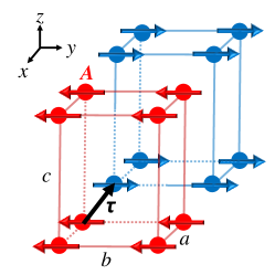
Figure 1: The schematic structure of the FeSb₂ crystal in the orthorhombic configuration that gives rise to the altermagnetism. The Fe atoms at the two magnetic sublattices, $A$ and $B$ are shown by the red and blue spheres. The magnetization on Fe atoms shown by red and blue arrows is (anti)-aligned with the easy $\hat{y}$ axis. The Sb (not shown) form a cage for Fe atoms distorted differently at the two sublattices.

Although $\mathcal{T}$ symmetry is broken, the combined $\mathcal{T}C_{2z}$ operation remains the symmetry with and without the SO interaction. Here $C_{2x_{i}}$ denotes a two-fold rotation around the $x_{i}=x,y,z$ coordinate axis. The antiunitary symmetry, $\mathcal{T}C_{2z}$ imposes the restrictions, $\sigma_{xy}=\sigma_{yx}$, $\sigma_{xz}=-\sigma_{zx}$ and $\sigma_{yz}=-\sigma_{zy}$ on the conductivity tensor, $\sigma$. This implies at most the transport anisotropy in the $xy$-plane in the form of the planar Hall effect, yet no AHE as $\sigma^{H}_{xy}=(\sigma_{xy}-\sigma_{yx})/2=0$. In contrast, unless forbidden by other symmetries $\mathcal{T}C_{2z}$ makes the Hall conductivity, $\sigma^{H}_{xz}$ and $\sigma^{H}_{yz}$ symmetry allowed. We investigate the necessary conditions as well as the way to compute the anomalous Hall response for a particular class of altermagnets.

In some phenomena such as a characteristic $\pi$-transitions in altermagnet Josephson junction, the SO interaction is inessential [14]. However, this is not so for AHE as well as other transport and optical phenomena. Our approach to AHE is to include the SO interaction from the start. To this end, we deduce a minimal tight-binding model constrained by the nontranslation symmetry operations forming a magnetic symmetry (factor) group, $\mathcal{G}_{M}$. Half of the elements of $\mathcal{G}_{M}$ constitute a unitary subgroup, $\mathcal{G}$. At finite SO interaction and for the magnetization collinear with the $\hat{y}$ direction, $\mathcal{G}=\{E,\mathcal{P},\boldsymbol{\tau}C_{2x},\boldsymbol{\tau}\sigma_{x}\}$, where $E$ is identity operation, $\sigma_{x}=\mathcal{P}C_{2x}$ is a mirror in $yz$-plane. The remaining half of the elements of $\mathcal{G}_{M}$ consists of the antiunitary operations, $\mathcal{T}C_{2z}\mathcal{G}$. Symbolically, $\mathcal{G}_{M}=\mathcal{G}+\mathcal{T}C_{2z}\mathcal{G}$.

The spins of conduction electrons couple to the local staggered magnetization. To model this coupling we introduce the exchange field, $\pm B_{ex}\hat{y}$ alternating between the two sublattices. Hence, the exchange field causes the energy spin splitting, $2B_{ex}$ of the localized electron states. Any model of the band structure has to be constrained by the symmetry. We now list these constraints.

When both the SO interaction and the magnetization are set to zero, the bands become doubly degenerate due to the full spin SU(2) invariance. In this, most symmetric situation the symmetry may give rise to the extra degeneracies not related to the spin for $\mathbf{k}\in\mathcal{K}_{0}$. In our problem, for the symmetry group $\mathcal{G}_{M}$, the set $\mathcal{K}_{0}$ includes the $k_{y}=\pi$ plane, as well as the two lines, $k_{x}=0$, $k_{z}=\pi$ and $k_{x}=\pi$, $k_{z}=0$. The total degeneracy including spin at $\mathbf{k}\in\mathcal{K}_{0}$ is four. This extra degeneracy is a consequence of the antiunitary symmetries. It follows straightforwardly by applying the Wigner criterion to the single-valued representations.

At the other extreme, when both SO interaction and the exchange field are present the $\mathcal{G}_{M}$ symmetry gives rise to the double degeneracy for momenta $\mathbf{k}\in\mathcal{K}_{\mathrm{SO}}$. For the $\mathcal{G}_{M}$ symmetry group, $\mathcal{K}_{\mathrm{SO}}=\mathcal{K}_{0}$. The total degeneracy at $\mathbf{k}\in\mathcal{K}_{\mathrm{SO}}$ is two. And, again it follows from the Wigner criterion, this time applied to the the double-valued representations.

In the intermediate situation when SO interaction is zero, while the exchange is finite the application of the spin symmetries results in the double degeneracy surviving the exchange field for $\mathbf{k}\in\mathcal{K}_{\mathrm{alt}}$. In addition to $\mathcal{K}_{\mathrm{SO}}$, $\mathcal{K}_{\mathrm{alt}}$ includes the two planes, $k_{x}=0$ and $k_{y}=0$. The degeneracies at $\mathbf{k}\in\mathcal{K}_{\mathrm{alt}}-\mathcal{K}_{\mathrm{SO}}$ appear as accidental from the point of view of a standard symmetry analysis. They, in fact, are systematic within the extended spin symmetry analysis. We point out, however, that within our approach the standard classification is sufficient to identify the set, $\mathcal{K}_{\mathrm{alt}}$.

We consider a single orbital model which generically gives rise to the four bands originating from the two sublattices and the two spin components. The model, in principle, does not assume the exchange splitting to be larger than the SO interaction. Yet, when this is the case the calculation of the Hall coefficient greatly simplifies. If $2B_{ex}$ is the dominant energy scale, the original four bands split into two pairs of bands that are vastly separated in energy. In both cases, we can safely ignore the on-site SO coupling compared to the exchange splitting.

The paper is organized as follows. In Sec. II we construct the minimal tight-binding model capturing the essential features of the SO coupled altermagnet with $\mathcal{G}_{M}$ symmetry group. Next, we check the consistency of the resulting band structure with the general symmetry requirements in Sec. III. The AHE is computed for an effective two-band model valid at large exchange splitting in Sec. IV. Finally, we summarize the results in Sec. V. In this section, we give a broader perspective including the most obvious future research directions that become accessible as a result of this work.

II Single orbital tight-binding model

We construct the simplest tight-binding model of itinerant electrons to incorporate the SO coupling in an altermagnet. We start with the atomic limit by looking at the effect of the lattice on electronic states localized at a given lattice site. The exchange splitting, $2B_{ex}$ is assumed to be much larger than the spin splitting induced by the SO interaction locally at a given site. It makes it reasonable to ignore the local effect of the SO interaction. In contrast, we do study in detail the effect of SO interaction on the hopping amplitudes to the neighboring sites in the following sections.

In the absence of the local SO interaction the spin and orbital degrees of freedom at a given site are decoupled. We, hence can momentarily ignore the spin and discuss the localized orbital wave-functions. The symmorphic symmetry operations acting within a given sublattice form an Abelian subgroup. The Sb ions forming a cage around Fe sites lift the orbital degeneracy. Hence we are allowed to focus on a single orbital wave-function at the $A$ and $B$ sublattices, $\phi_{A(B)}(\mathbf{r})$.

The nonsymmorphic $\boldsymbol{\tau}C_{2x}$ symmetry implies the relationship $\phi_{B}(\mathbf{r})=\phi_{A}(C_{2x}^{-1}\mathbf{r})$. At finite $B_{ex}$ the two sets of degenerate pseudospin states possessing the same orbital wave function $\phi_{A(B)}(\mathbf{r})$ are $\{\phi_{A}(\mathbf{r})\chi_{+},\phi_{B}(\mathbf{r})\chi_{-}\}$ and $\{\phi_{B}(\mathbf{r})\chi_{+},\phi_{A}(\mathbf{r})\chi_{-}\}$. Here $\chi_{\pm}$ are spinors for the states polarized along $\pm\hat{y}$ direction fixed by the staggered magnetization, $\hat{s}_{y}\chi_{\pm}=\pm\chi_{\pm}$, where $\hat{\mathbf{s}}$ is electron spin operator. Specifically, $\chi_{\pm}=(\bar{\chi}_{\uparrow}\pm i\bar{\chi}_{\downarrow})/\sqrt{2}$, where $\hat{s}_{z}\bar{\chi}_{\uparrow(\downarrow)}=\pm\bar{\chi}_{\uparrow(\downarrow)}$. These relations define the transformation matrix, $\chi_{s}=\sum_{\sigma=\uparrow,\downarrow}S_{\sigma s}\bar{\chi}_{\sigma}$.

Figure 2: (a) The symmetry-allowed hybridization of the $s$ and $d_{xy}$ orbitals at Fe sites. The hybridized wave functions at the $A$ and $B$ sublattices are related by the nonsymmorphic $\boldsymbol{\tau}C_{2x}$ symmetry operation. As a result, the hybridized orbital wave function at the two sublattices are distinct. (b) The consequence of the difference in the orbital wave function for the two sublattices is a finite $A^{\prime}$ in Eq. (16) causing a spin splitting even at zero SO interaction. The projection of the crystal structure on the $xy$-plane is shown.

It is crucial for the altermagnetism that the functional form of the $\phi_{A}(\mathbf{r})$ and $\phi_{B}(\mathbf{r})$ orbital wave functions of the two members in each degenerate doublet may differ. Indeed the on-site symmetry allows the orbitals of the same parity that are both even or odd with respect to $C_{2z}$ to hybridize. This makes room for the hybridization of orbitals transforming differently under $C_{2x}$. For instance, the hybridization of $s$- and $d_{xy}$-orbitals gives rise to distinct orbital wave functions at the two sublatices, see Fig. 2a. This point is further elaborated upon in Sec. II.2.

When the two degenerate doublets are split by a strong $B_{ex}$ the effective two-band model may suffice to describe the band structure. Here, however, we retain all four bands in order to address the regime of the exchange splitting comparable to the band width. Besides, it allows us to clarify the limitations of the effective two-band description. Technically, we have to work with the full space in order to explore all the limitations imposed by symmetry.

These considerations naturally lead us to the tight-binding four band model of the form,

$$\mathcal{H}=\sum_{\mathbf{k}}\Psi_{\mathbf{k}\alpha}^{\dagger}\hat{H}_{\alpha\beta}(\mathbf{k})\Psi_{\mathbf{k}\beta}\,,$$ (1)

expressed in terms of the generalized Nambu spinor,

$$\Psi^{\dagger}_{\mathbf{k}}=\left[\psi^{\dagger}_{\mathbf{k}A+},\psi^{\dagger}_{\mathbf{k}B+},\psi^{\dagger}_{\mathbf{k}A-},\psi^{\dagger}_{\mathbf{k}B-}\right]\,.$$ (2)

When applied to vacuum, $|0\rangle$, $\psi^{\dagger}_{\mathbf{k}As}$ and $\psi^{\dagger}_{\mathbf{k}Bs}$ create the electronic Bloch states localized at the $A$- and $B$-sublattices, respectively with the $s=\pm$ spin projection on the magnetization direction. Specifically,

$$\psi^{\dagger}_{\mathbf{k}As}|0\rangle =\frac{1}{\sqrt{N}}\sum_{\mathbf{R}\in A}e^{i\mathbf{k}\mathbf{R}}\phi_{A}(\mathbf{r}-\mathbf{R})\chi_{s}\,,$$ (3a)

$$\psi^{\dagger}_{\mathbf{k}Bs}|0\rangle =\frac{1}{\sqrt{N}}\sum_{\mathbf{R}\in A}e^{i\mathbf{k}\mathbf{R}}\phi_{B}(\mathbf{r}-\mathbf{R}-\boldsymbol{\tau})\chi_{s}\,,$$ (3b)

where $N$ Fe ions of the $A$-sublattice are located at the cites of the orthorhombic lattice, $\mathbf{R}=n_{x}a\hat{x}+n_{y}b\hat{y}+n_{z}c\hat{z}$ defined by the three integers, $n_{x,y,z}$. Hereinafter, the distances along the three crystallographic directions are measured in units of $a$, $b$ and $c$, respectively. Correspondingly, the momentum components $k_{x,y,z}$ are measured in units of $a^{-1}$, $b^{-1}$ and $c^{-1}$.

To parametrize the Hamiltonian in Eq. (1) we introduce the two sets of Pauli matrices, $\boldsymbol{\varkappa}$ and $\boldsymbol{\sigma}$ acting in sublattice and spin spaces, respectively. The unit matrices acting in these spaces are denoted as $\varkappa_{0}$ and $\sigma_{0}$, respectively. We write $\hat{H}(\mathbf{k})=\hat{H}_{ex}(\mathbf{k})+\hat{H}_{TB}(\mathbf{k})$, where the exchange part is $\hat{H}_{ex}=B_{ex}\varkappa_{z}\sigma_{z}$. The tight-binding part is split into the intra- and inter-sublattice hopping matrix elements, $\hat{H}_{TB}(\mathbf{k})=\hat{H}^{a}(\mathbf{k})+\hat{H}^{e}(\mathbf{k})$, respectively. Furthermore, the minimal generic model free of accidental degeneracies includes the nearest neighbor hopping processes contribution to $\hat{H}^{e}(\mathbf{k})$, and the contribution of the next nearest hopping processes within the same sublattice to $\hat{H}^{a}(\mathbf{k})=\hat{H}^{a}_{n}(\mathbf{k})+\hat{H}^{a}_{nn}(\mathbf{k})$. Below we obtain the generic form of these terms constrained by the $\mathcal{G}_{M}$ symmetry.

II.1 Nearest neighbor inter-sublattice hopping processes

We start with the analysis of $\hat{H}^{e}(\mathbf{k})$ part of the tight-binding Hamiltonian. The real space hopping matrix elements of the full microscopic space periodic Hamiltonian, $H$ are introduced in a standard way,

$$\bar{T}^{\sigma^{\prime}\sigma}_{BA}(\boldsymbol{\tau}_{\mathbf{n}})=\langle\phi_{B}(\mathbf{r}-\boldsymbol{\tau}_{\mathbf{n}})\bar{\chi}_{\sigma^{\prime}}|H|\phi_{A}(\mathbf{r})\bar{\chi}_{\sigma}\rangle\,.$$ (4)

A given $A$ site has eight neighboring sites to hop to in the $B$-sublattice with the hopping vectors, $\boldsymbol{\tau}_{\mathbf{n}}=(1/2)(n_{x}\hat{x}+n_{y}\hat{y}+n_{z}\hat{z})$ fixed by the choice of $n_{x,y,z}=\pm 1$. In particular, $\boldsymbol{\tau}_{\mathbf{n}}=\boldsymbol{\tau}$ for $n_{x}=n_{y}=n_{z}=1$. It is convenient to represent the spin dependence of amplitude Eq. (4) in the form,

$$\hat{\bar{T}}_{BA}(\boldsymbol{\tau}_{\mathbf{n}})=t_{0}(\boldsymbol{\tau}_{\mathbf{n}})\sigma_{0}+\mathbf{t}(\boldsymbol{\tau}_{\mathbf{n}})\cdot\boldsymbol{\sigma}\,.$$ (5)

We are interested in the hopping matrix elements in the $\chi_{s}$ basis, $T^{s^{\prime}s}_{BA}(\boldsymbol{\tau}_{\mathbf{n}})$ defined similarly to Eq. (4). The two are related by the transformation, $\hat{T}_{BA}(\boldsymbol{\tau}_{\mathbf{n}})=S^{-1}\hat{\bar{T}}_{BA}(\boldsymbol{\tau}_{\mathbf{n}})S$. It follows that $\hat{T}_{BA}(\boldsymbol{\tau}_{\mathbf{n}})$ is obtained from Eq. (5) by cyclic transformation of $\{\sigma_{x},\sigma_{y},\sigma_{z}\}$ into $\{\sigma_{y},\sigma_{z},\sigma_{x}\}$.

In Eq. (5) the second spin-dependent term describes the effect of SO interaction. Our strategy to deal with the zero SO limit is, therefore, to set the vector part of Eq. (5) to zero, $\mathbf{t}(\boldsymbol{\tau}_{\mathbf{n}})=0$. Strictly speaking, one has to eliminate the terms that do not commute with the exchange interaction. Yet, as we show explicitly this distinction makes no difference. In Sec. III we explicitly demonstrate that the spectral degeneracies obtained in this way are exactly the same as predicted by the extended spin symmetry approach.

We now turn to the constrains imposed on the matrix elements Eq. (4) by $\mathcal{G}_{M}$ symmetry. The parity symmetry $\mathcal{P}$ imposes the condition,

$$\hat{\bar{T}}_{BA}(\boldsymbol{\tau}_{\mathbf{n}})=\hat{\bar{T}}_{BA}(-\boldsymbol{\tau}_{\mathbf{n}})\,.$$ (6)

The unitary symmetry $\boldsymbol{\tau}C_{2x}$ imposes the constrain,

$$\hat{\bar{T}}_{BA}(\boldsymbol{\tau}_{\mathbf{n}})=\sigma_{x}[\hat{\bar{T}}_{BA}(C_{2x}\boldsymbol{\tau}_{\mathbf{n}})]^{\dagger}\sigma_{x}\,.$$ (7)

The antiunitary symmetry $C_{2z}\mathcal{T}$ leads to the condition,

$$\hat{\bar{T}}_{BA}(\boldsymbol{\tau}_{\mathbf{n}})=\sigma_{x}[\hat{\bar{T}}_{BA}(C_{2z}\boldsymbol{\tau}_{\mathbf{n}})]^{*}\sigma_{x}\,.$$ (8)

Applying the set of the three equations (6), (7) and (8) to Eq. (5) yields the following constrains,

$$t_{0,x}(\boldsymbol{\tau}_{\mathbf{n}})\!=\!t_{0,x}(-\boldsymbol{\tau}_{\mathbf{n}})\!=\!t^{*}_{0,x}(C_{2x}\boldsymbol{\tau}_{\mathbf{n}})\!=\!t^{*}_{0,x}(C_{2z}\boldsymbol{\tau}_{\mathbf{n}}),$$ (9a)

$$t_{z}(\boldsymbol{\tau}_{\mathbf{n}})=t_{z}(-\tau_{i})=-t^{*}_{z}(C_{2x}\boldsymbol{\tau}_{\mathbf{n}})=-t^{*}_{z}(C_{2z}\boldsymbol{\tau}_{\mathbf{n}})\,,$$ (9b)

$$t_{y}(\boldsymbol{\tau}_{\mathbf{n}})=0\,.$$ (9c)

Equation (9) implies that the $\mathcal{G}_{M}$ reduces the 32 complex parameters in Eq. (4) down to 3. We take for these parameters, $t_{0}=t_{0}(\boldsymbol{\tau})$, $t_{x}=t_{x}(\boldsymbol{\tau})$ and $t_{z}=t_{z}(\boldsymbol{\tau})$. All the other hopping amplitudes follow from Eq. (9) as summarized in Tab. 1.

Table 1: The nearest neighbor inter-sublattice hopping parameters constrained by Eq. (9). The four out of eight hopping vectors, $\boldsymbol{\tau}_{\mathbf{n}}=\mathbf{n}/2$ are sufficient in view of Eq. (6), and $\boldsymbol{\tau}_{-\mathbf{n}}=-\boldsymbol{\tau}_{\mathbf{n}}$. The Bravais lattice vector, $\Delta\mathbf{R}(\boldsymbol{\tau}_{\mathbf{n}})$ is introduced in Eq. (11). For the neighboring sites that are not shown it is given by, $\Delta\mathbf{R}(-\boldsymbol{\tau}_{\mathbf{n}})=-\hat{x}-\hat{y}-\hat{z}-\Delta\mathbf{R}(\boldsymbol{\tau}_{\mathbf{n}})$.

$\mathbf{n}$	$(1,1,1)$	$(-1,1,1)$	$(1,-1,1)$	$(1,1,-1)$
$t_{0,x}(\mathbf{\tau}_{\mathbf{n}})$	$t_{0,x}$	$t^{*}_{0,x}$	$t_{0,x}$	$t^{*}_{0,x}$
$t_{z}(\mathbf{\tau}_{\mathbf{n}})$	$t_{z}$	$-t^{*}_{z}$	$t_{z}$	$-t^{*}_{z}$
$\Delta\mathbf{R}$	$0$	$-\hat{x}$	$-\hat{y}$	$-\hat{z}$

The tight-binding Hamiltonian resulting from the inter-sublattice hopping processes,

$$\hat{H}_{e}(\mathbf{k})=\varkappa_{-}\hat{T}_{BA}(\mathbf{k})+\varkappa_{+}\hat{T}^{\dagger}_{BA}(\mathbf{k})\,,$$ (10)

where $\varkappa_{\pm}=(\varkappa_{x}\pm i\varkappa_{y})/2$, and the hopping amplitude in the Fourier space are determined by the substitution of Eqs. (3) into the hopping integral, Eq. (4),

$$\hat{T}_{BA}(\mathbf{k})=\sum_{\boldsymbol{\tau}_{\mathbf{n}}}e^{-i\mathbf{k}\Delta\mathbf{R}(\boldsymbol{\tau}_{\mathbf{n}})}S^{-1}\hat{\bar{T}}_{BA}(\boldsymbol{\tau}_{\mathbf{n}})S\,,$$ (11)

where $\Delta\mathbf{R}(\boldsymbol{\tau}_{\mathbf{n}})$ is the Bravais lattice vector connecting the unit cells hosting the neighboring sites at $A$ and $B$ sublattices.

Table 2: The next nearest neighbor intra-sublattice hopping parameters constrained by the symmetry. The six out of twelve amplitudes are shown. The rest follows from the symmetry of all the amplitudes under reversal of $\Delta\mathbf{R}$.

$\Delta\mathbf{R}$	$\hat{x}+\hat{y}$	$\hat{x}-\hat{y}$	$\hat{y}+\hat{z}$	$\hat{y}-\hat{z}$	$\hat{z}+\hat{x}$	$\hat{z}-\hat{x}$
$T_{A}(\Delta\mathbf{R})$	$A_{+}$	$A_{-}$	$A_{1}$	$A_{1}$	$A_{2}$	$A_{2}$
$T_{B}(\Delta\mathbf{R})$	$A_{-}$	$A_{+}$	$A_{1}$	$A_{1}$	$A_{2}$	$A_{2}$

As the hopping amplitudes are parametrized as in Eq. (5), Eq. (11) yields

$$t_{0,x,z}(\mathbf{k})=\sum_{\boldsymbol{\tau}_{\mathbf{n}}}e^{-i\mathbf{k}\Delta\mathbf{R}(\boldsymbol{\tau}_{\mathbf{n}})}t_{0,x,z}(\boldsymbol{\tau}_{\mathbf{n}})\,.$$ (12)

The quantities needed to express the amplitudes, Eq. (12) are given in the Tab. 1. The resulting expressions read

$$t_{0,x} (\mathbf{k})=\left(1+e^{ik_{y}}\right)$$

$$\times \left\{t_{0,x}\left[1+e^{i(k_{x}+k_{z})}\right]+t^{*}_{0,x}\left(e^{ik_{x}}+e^{ik_{z}}\right)\right\}\,,$$ (13a)

$$t_{z}(\mathbf{k}) =\left(1+e^{ik_{y}}\right)$$

$$\times \left\{t_{z}\left[1+e^{i(k_{x}+k_{z})}\right]-t^{*}_{z}\left(e^{ik_{x}}+e^{ik_{z}}\right)\right\}\,.$$ (13b)

Equations (10) through (13) fix the inter-sublattice contribution to the tight-binding Hamiltonian, $\hat{H}_{e}(\mathbf{k})$.

II.2 Intra-sublattice hopping processes

We now turn to the intra-sublattice part of the tight-binding Hamiltonian, $\hat{H}^{a}(\mathbf{k})$. Consider first the nearest neighbor hopping amplitudes, $\hat{H}^{a}_{n}(\mathbf{k})$. Since we have just accounted for the SO coupling, at this level we consider only the spin-independent components of hopping amplitudes. The symmetry arguments similar to the presented above results in the nearest-neighbor contribution of the form, $\hat{H}^{a}_{n}(\mathbf{k})=\varkappa_{0}\sigma_{0}H^{a}_{n}(\mathbf{k})$ with

$$H^{a}_{n}(\mathbf{k})=a_{x}\cos k_{x}+a_{y}\cos k_{y}+a_{z}\cos k_{z}\,,$$ (14)

where $a_{x,y,z}$ are three real parameters.

In the limit of small SO interaction, the Hamiltonian in Eq.(14) produces the same spin degeneracy at all $\mathbf{k}$-points. Clearly, such degeneracy is accidental, and Eq. (14) is not generic enough. It makes it necessary to consider the next-nearest neighbors hopping amplitudes. We again neglect any spin dependent contributions, and focus on the spin scalar part of the hopping amplitude,

$$T_{A}(\mathbf{R}_{m})=\frac{1}{2}\sum_{\sigma}\langle\phi_{A}(\mathbf{r}-\mathbf{R}_{m})\bar{\chi}_{\sigma}|H|\phi_{A}(\mathbf{r})\bar{\chi}_{\sigma}\rangle\,$$ (15)

with the similar definition for $T_{B}(\mathbf{R}_{m})$. In equation (15) the vector $\mathbf{R}_{m}$ can take one of the twelve possible values, $m_{1}\hat{x}+m_{2}\hat{y}$, $m_{1}\hat{y}+m_{2}\hat{z}$ and $m_{1}\hat{z}+m_{2}\hat{z}$ for $m_{1,2}=\pm 1$. In this case the symmetry reduces the twenty four real parameters down to four, see Tab. 2. We denote, $T_{A}(\hat{x}\pm\hat{y})=A_{\pm}$, $T_{B}(\hat{x}\pm\hat{y})=A_{\mp}$, with all the rest of the amplitudes being equal on the two sublattices.

The feature essential for the altermagnetism is $A_{+}\neq A_{-}$. This allows for the spin polarization to be controlled by the staggered magnetization and not by the SO interaction. In what follows we retain only the essential part of the next to nearest neighbor interaction by setting, $A_{+}=-A_{-}=A^{\prime}$. As a result we have the following contribution,

$$\hat{H}^{a}_{nn}(\mathbf{k})=A^{\prime}\varkappa_{z}f_{2}(\mathbf{k})$$ (16)

expressed via the function,

$$f_{2}(\mathbf{k})=2\left[\cos(k_{x}+k_{y})-\cos(k_{x}-k_{y})\right]\,.$$ (17)

When combined Eqs. (14) and (16) define the intra-sublattice part of the Hamiltonian, $\hat{H}^{a}(\mathbf{k})$.

Qualitatively, the emergence of the finite spin splitting at zero SO interaction results from the difference in the orbital wave function for the two sublattices as shown in Fig. 2b.

II.3 Effective two-band model

To clarify the role of the SO interaction in transport we study the limit of a large exchange field. When the exchange splitting exceeds the bandwidth the two subspaces, $V_{+}=\{\phi_{A}(\mathbf{r})\chi_{+},\phi_{B}(\mathbf{r})\chi_{-}\}$ and $V_{-}=\{\phi_{A}(\mathbf{r})\chi_{-},\phi_{B}(\mathbf{r})\chi_{+}\}$ approximately decouple. Neglecting all the terms of the Hamiltonian, $\hat{H}(\mathbf{k})$ that mix the two spaces we have the following two effective Hamiltonians,

$$H_{u(d)}\!=\!\begin{bmatrix}H_{n}^{a}\!\pm\!B_{ex}\!+\!A^{\prime}\!f_{2}(\mathbf{k})&t_{z}^{*}(\mathbf{k})\mp it_{x}^{*}(\mathbf{k})\\ t_{z}(\mathbf{k})\pm it_{x}(\mathbf{k})&H_{n}^{a}\!\pm\!B_{ex}\!-\!A^{\prime}\!f_{2}(\mathbf{k})\end{bmatrix}$$ (18)

acting in the $V_{\pm}$-subspaces, respectively. The two Hamiltonians, $H_{u(d)}$ are very similar, and it is enough to focus on one of them, say $H_{u}$.

III Symmetries and band degeneracies

It is crucial to make sure that our model satisfies all the symmetry requirements. The set of momenta, $\mathcal{K}_{\mathrm{SO}}$ at which bands are doubly degenerate at finite exchange and SO interactions has been spelled out in Ref. [9]. The reason we sketch the alternative derivation is to identify the degeneracies also in the spin SU(2) invariant limit imposed by the $\mathcal{G}_{M}$ symmetry. This limit is of interest for us here as it sets an additional constrains our model has to satisfy.

III.1 General symmetry imposed constrains

In the present problem, the Wigner criterion states that for a given $\mathbf{k}$ one has to compute the sum to distinguish between the three cases,

$$\sum^{\prime}_{g\in\mathcal{G}}\chi^{\mathbf{k}}\left[(C_{2z}g)^{2}\right]=\begin{cases}+[\mathbf{k}]\mathcal{T}^{2}&\mathrm{case\,(a)}\\ -[\mathbf{k}]\mathcal{T}^{2}&\mathrm{case\,(b)}\\ 0&\mathrm{case\,(c)}\end{cases}\,.$$ (19)

In the case (a) the antiunitary operation, $C_{2z}\mathcal{T}$ does not cause the extra degeneracy, and in cases (b) and (c) it does. The band degeneracy, in addition, requires that there are elements $g\in\mathcal{G}$ such that $C_{2z}g$ reverses the momentum [15, 16]. The summation in Eq. (19) only runs over $[\mathbf{k}]$ such elements. The $\chi^{\mathbf{k}}$ is the irreducible character of the group of $\mathbf{k}$, $\mathcal{G}_{\mathbf{k}}$.

Consider for illustration the generic point in the $k_{y}=\pi$ plane, $\mathbf{k}=(k_{x},\pi,k_{z})$. For generic $k_{x}$ and $k_{z}$, the group $\mathcal{G}_{\mathbf{k}}$ contains just the translations, $\mathbf{R}$. The sum in Eq. (19) contains just a single term, $g=\mathbf{\tau}C_{2x}$, $[\mathbf{k}]=1$. And since this operation squares to $(C_{2z}\mathbf{\tau}C_{2x})^{2}=-\mathbf{R}_{y}C_{2y}^{2}$ with $\mathbf{R}_{y}=\hat{y}$, the sum in the Wigner criterion is trivially evaluated,

$$\chi^{\mathbf{k}}\left[(C_{2z}g)^{2}\right]=-\mathcal{T}^{2}\,.$$ (20)

Indeed, $C_{2y}^{2}=\mathcal{T}^{2}=\mp 1$ for (half)-integer spin, and according to Bloch theorem, $\chi^{\mathbf{k}}(\mathbf{R})=\exp(-i\mathbf{k}\mathbf{R})$. Based on Eq. (20) we conclude that the degeneracy of Bloch bands at $k_{y}=\pi$ doubles due to the $C_{2z}\mathcal{T}$ antiunitary symmetry both for the SU(2) invariant and finite SO interaction cases. Similar analysis shows that this statement holds true for all $\mathbf{k}\in\mathcal{K}_{\mathrm{SO}}$.

III.2 The symmetry, and the tight-binding model

We now benchmark our model Hamiltonian, Eq. (1) with the generic symmetry requirements outlined in Sec. III.1. The term $\hat{H}_{n}^{a}(\mathbf{k})\propto\varkappa_{0}\sigma_{0}$, Eq. (14) does not affect the degeneracies and for better clarity, we focus on $\hat{H}^{\prime}=\hat{H}-\hat{H}_{n}^{a}$ instead. Clearly, in the absence of the SO interaction the spin states $|\pm\rangle$ decouple,

$$\hat{H}^{\prime}(\mathbf{k})=\begin{bmatrix}M_{+}(\mathbf{k})&0\\ 0&M_{-}(\mathbf{k})\end{bmatrix}\,,$$ (21)

where according to Eqs. (16),

$$M_{\pm}=\begin{bmatrix}\pm B_{ex}+A^{\prime}f_{2}(\mathbf{k})&t_{0}^{*}(\mathbf{k})\\ t_{0}(\mathbf{k})&\mp B_{e}-A^{\prime}f_{2}(\mathbf{k})\end{bmatrix}\,.$$ (22)

We now explore the band degeneracies of the SO free Hamiltonian, Eq. (21). The spectrum contains four branches, $E_{1,2}=\pm\sqrt{(B_{ex}+A^{\prime}f_{2}(\mathbf{k}))^{2}+|t_{0}(\mathbf{k})|^{2}}$ for the $M_{+}$ branch and $E_{3,4}=\pm\sqrt{(B_{ex}-A^{\prime}f_{2}(\mathbf{k}))^{2}+|t_{0}(\mathbf{k})|^{2}}$ for the $M_{-}$ branch.

In the limit of $B_{ex}=0$ and zero SO interaction the system is spin SU(2) invariant. Wigner criterion gives the degeneracies beyond the trivial spin up/down one for $\mathbf{k}\in\mathcal{K}_{SO}$. This is exactly what follows from the above dispersion relations. Indeed, at $B_{ex}=0$ we have $E_{1(2)}=E_{3(4)}$ and the extra degeneracy implies $f_{2}=f_{1}=0$ which only happens for $\mathbf{k}\in\mathcal{K}_{SO}$.

Next we set $B_{ex}\neq 0$. Even though we are still in the limit of zero SO interaction the problem is not spin SU(2) invariant. Naively, based on the discussion in Sec. III.1 one expects spin degeneracy again at $\mathbf{k}\in\mathcal{K}_{SO}$. From our dispersion relations we see that the degeneracy that does not depend on a particular value of $B_{ex}$ requires $f_{2}=0$. This relationship is satisfied for $\mathbf{k}\in\mathcal{K}_{\mathrm{alt}}$. The set, $\mathcal{K}_{SO}$ is a proper subset of $\mathcal{K}_{\mathrm{alt}}$. The extra degeneracy not accounted for by our Wigner criterion emerges as the actual group of symmetry operations, referred to as spin symmetry group by Ref.[9] is larger than $\mathcal{G}_{M}$.

Finally, when both $B_{ex}$ and the SO interaction are non-zero, $t_{x}\neq 0$ and/or $t_{z}\neq 0$ the double degeneracy survives only at $\mathbf{k}\in\mathcal{K}_{\mathrm{SO}}$ in accordance with the Wigner criterion. In our particular model this follows from Eq. (13) and vanishing of $f_{1}(\mathbf{k})$ at $\mathbf{k}\in\mathcal{K}_{\mathrm{SO}}$ only.

IV Anomalous Hall effect

Here we apply the effective Hamiltonian Eq. (18) to study the Hall response of the SO coupled altermagnet. In this work we limit the consideration to the intrinsic contribution. The standard expression for the intrinsic part of the anomalous Hall effect [17, 18],

$$\sigma^{H}_{ij}=e^{2}\sum^{\prime}_{b\mathbf{k}}\Omega^{b}_{ij}(\mathbf{k})$$ (23)

relates it to the Berry curvature antisymmetric tensor $\Omega^{b}_{ij}$. At zero temperature the primed summation in Eq. (23) runs over all occupied Bloch momenta at all the partially or fully filled bands, labeled by $b$. The Berry curvature tensor is defined as $\Omega^{b}_{ij}(\mathbf{k})=-2\mathrm{Im}\langle\partial_{k_{i}}u_{b}(\mathbf{k})|\partial_{k_{i}}u_{b}(\mathbf{k})\rangle$, where $u_{b}(\mathbf{k})$ are periodic parts of the Bloch functions, at the band $b$ and momentum $\mathbf{k}$.

To get an understanding of what parts of the Hamiltonian, Eq. (18) are essential, we parametrize it via the set $\boldsymbol{\rho}$ of Pauli matrices operating in the $V_{+}$ space in a standard way,

$$H^{e}_{u}(\mathbf{k})=-\mathbf{h}(\mathbf{k})\cdot\boldsymbol{\rho}\,.$$ (24)

Since only the wave functions and not the spectrum enters the expression for the Berry curvature [Eq. (23)] in Eq. (24) we have set to zero the exchange field and the nearest neighbor intra-sublattice hopping terms, $B_{ex}=0$ and $H_{n}^{a}=0$.

Such terms, however are the most important in determining the region of summation in Eq. (23). Indeed, at a given momentum, $\mathbf{k}$ the two bands arising from the effective Hamiltonian, Eq. (18), produce the opposite Berry curvature. Therefore, the momenta that contribute to the Hall conductivity in Eq. (23) are such that the lower band is occupied and the upper band is empty. In other words the integration region in Eq. (23) is squeezed in between the two Fermi surfaces of the above two bands.

It is, therefore sufficient to present the Bloch periodic part of the wave-function of the lower of the two bands in the form,

$$|u_{h}(\mathbf{k})\rangle=\begin{pmatrix}\cos(\theta_{\mathbf{k}}/2)\\ \sin(\theta_{\mathbf{k}}/2)e^{i\varphi_{\mathbf{k}}+i\mathbf{k}\boldsymbol{\tau}}\end{pmatrix}\,,$$ (25)

where $\theta_{\mathbf{k}}$ and $\varphi_{\mathbf{k}}$ are the spherical angles fixing the direction of $\mathbf{h}$ in Eq. (24). The extra-phase $\mathbf{k}\boldsymbol{\tau}$ in the spinor, Eq. (25) is needed as per our definition of the Bloch states, Eq. (3), the periodic part of the wave function at the $B$ sites is phase shifted by $\mathbf{k}\boldsymbol{\tau}$ with respect to the A sites.

We consider the set of parameters resulting in a small Fermi surface centered at the $\Gamma$ point. This allows us to work with the $\mathbf{k}\cdot\mathbf{p}$ Hamiltonian by the series expansion of our effective Hamiltonian, Eq. (24). In terms of the real and imaginary parts, $t_{x,z}^{r,i}$ of the SO parameters, $t_{x,z}$ the two independent expansion parameters of the SO interaction are $t_{1}=t_{z}^{i}+t_{x}^{r}$ and $t_{2}=t_{z}^{r}-t_{x}^{i}$. Accordingly, we keep only the leading terms in both of them to arrive at the Hamiltonian,

$$h_{x}=2t_{2}k_{x}k_{z}\,,h_{y}=-8t_{1}\,,h_{z}=4A^{\prime}k_{x}k_{y}\,.$$ (26)

We start with the $\sigma^{H}_{xy}$. The straightforward calculation of the Berry curvature based on Eqs. (25) and (26) yields

$$\frac{\Omega_{xy}(\mathbf{k})}{a^{2}}=\frac{A^{\prime}ak_{x}\left(a^{4}k_{x}^{2}k_{z}^{2}t_{2}^{2}+8ak_{z}t_{1}t_{2}+16t_{1}^{2}\right)}{\left[k_{x}^{2}\left(4A^{\prime 2}a^{2}k_{y}^{2}+a^{2}k_{z}^{2}t_{2}^{2}\right)+16t_{1}^{2}\right]^{3/2}},$$ (27)

where we have restored the original units of the momentum, and assumed $a_{x,y,z}=a$ for simplicity. The Berry curvature, Eq. (27) integrates to zero, and $\sigma^{H}_{xy}=0$. To see this notice that $\Omega_{xy}(\mathbf{k})$ is odd in $k_{x}$. In contrast, the integration region in Eq. (23) is symmetric in all three components of $\mathbf{k}$. This, in turn follows from the symmetry of the energy spectrum of the Hamiltonian Eq. (18). Indeed, $H^{a}_{n}(\mathbf{k})$, Eq. (14) is even in each of the three momentum components. It can be checked based on Eqs. (13) and (16) that the same is true for $|t_{z}(\mathbf{k})+it_{z}(\mathbf{k})|^{2}$ and $|A^{\prime}f_{2}(\mathbf{k})|^{2}$, respectively. This shows that the spectrum of Eq. (18) possesses the aforementioned symmetry.

Similar arguments leads to $\sigma^{H}_{xz}=0$. The nonzero $\sigma^{H}_{yz}$ arises from the Berry curvature,

$$\Omega_{yz}(\mathbf{k})=\frac{8A^{\prime}a^{4}k_{x}^{2}t_{1}t_{2}}{\left[a^{2}k_{x}^{2}\left(4A^{\prime 2}a^{2}k_{y}^{2}+a^{2}k_{z}^{2}t_{2}^{2}\right)+16t_{1}^{2}\right]^{3/2}}\,.$$ (28)

Here we have omitted the terms that vanish upon the momentum integration. Such terms results from the extra phase $\mathbf{k}\boldsymbol{\tau}$ added to the spinor Eq. (25).

Figure 3: (a) The closed loop traversed by the $\mathbf{k}$ in the $yz$-plane at some fixed, $k_{x}\neq 0$. (b) As the vector, $\mathbf{k}$ follows the loop in panel (a), the vector $\mathbf{h}(\mathbf{k})$ defining the effective Hamiltonian, Eq. (24) and given by Eq. (26) encloses a loop in the space of $\mathbf{h}$ coordinates that subtends a finite solid angle, provided $A^{\prime}\neq 0$ and SO interaction is finite. This loop is the same for $\pm k_{x}$. Hence $\sigma^{H}_{yz}$ is finite.

In general, the calculation of the Hall conductivity has to be done numerically. Here as an illustration, we consider the metallic regime with the Fermi energy set by $B_{ex}$ and $H_{n}^{a}$ being considerably larger than the SO interaction. In this regime the integration volume in Eq. (23) is a tiny fraction of the volume enclosed by the Fermi surface. Furthermore, we assume that $t_{2}$ parameter dominates the energy splitting. In this case we have for the intrinsic Hall contribution,

$$\sigma^{H}_{yz}=\frac{4\pi e^{2}}{3}(k_{F}a)^{4}\frac{A^{\prime}}{v_{F}}\frac{t_{2}}{t_{1}}\,.$$ (29)

As is clear from the expression for the Berry curvature Eq. (28), the final result is obtained only for a finite $A^{\prime}$ and sufficiently generic SO interaction $t_{1,2}\neq 0$. The intra-sublattice nearest neighbor hopping terms $\propto A^{\prime}$ ensure the spin polarization at zero SO interaction. It is necessary, and yet insufficient condition for a finite anomalous Hall. Only in combination with the generic SO coupling a nontrivial winding of the spin texture in the Brillouin Zone results in a finite AHE.

This point can be understood also geometrically by following the evolution of the $\mathbf{h}(\mathbf{k})$ vector, Eq. (26) as $\mathbf{k}$ encloses a loop in the $yz$-plane defined by some fixed $k_{x}$. Such loop is shown in Fig. 3. It makes the $\mathbf{h}$ vector to transverse the closed loop in the space of $\mathbf{h}$ coordinates that subtends a finite solid angle. This latter loop is encircled in the same sense for both signs of $k_{x}$. This explains why both the SO coupling and the $A^{\prime}$ are needed for a finite AHE as well as relative positive sign of the contributions of positive and negative $k_{x}$.

The Hall effect as expressed by Eq. (29) does not have a well defined parity in $B_{ex}$. As $B_{ex}$ flips the sign the upper and lower bands defined in Eq. (18) switch. Per definitions used in writing Eq. (18) the parameter $A^{\prime}$ is the same for both bands. However the SO coupling $t_{x}$ changes sign. This means that the previous considerations have to be modified by changing $t_{1}$ and $t_{2}$ into $t^{\prime}_{1}=t_{z}^{i}-t_{x}^{r}$ and $t^{\prime}_{2}=t_{z}^{r}+t_{x}^{i}$. The parameters, $t_{1,2}$ and $t^{\prime}_{1,2}$ are generically unrelated. Therefore, the Hall conductivity does not have a well defined parity with respect to $B_{ex}$. As a result, it splits into odd and even components in $B_{ex}$. According to the classification of [1] these two components define AHE and crystal Hall effect, respectively. In the present model we have both contributions.

V Summary and Outlook

In this work, we have computed the intrinsic anomalous Hall effect of an altermagnet based on the minimal symmetry-constrained tight-binding model. Our method is based on the standard magnetic symmetry group. Strictly speaking, it applies only to finite SO interaction. To circumvent this limitation we eliminate all the terms describing the spin-flipping processes to reach the zero SO interaction limit. The resulting Hamiltonian produces the same spectrum degeneracies as required by the spin symmetry extended to include the operations acting differently on the spin and orbital degrees of freedom.

The model is free of accidental degeneracies only if the next-to-nearest neighbor intra-sublattice hopping processes are included. As the orbital structure of the states localized at the two sublattices is different these processes cause a well-defined spin polarization at zero SO coupling. Since the magnetism considered here is collinear the spin polarization alone does not produce a finite AHE. Our approach is perfectly sufficient to capture the most generic form of the SO coupling. We have shown that in combination with the spin polarization due to the staggered magnetization, it produces a finite AHE.

The considerations presented here are limited to the intrinsic contribution to AHE. Our model is general, and yet simple enough to serve as a starting point to explore the extrinsic contributions to AHE. One can expect the extrinsic contribution to dominate in the metallic regime where the Fermi energy exceeds the SO-induced gap.

References

- Šmejkal et al. [2020] L. Šmejkal, R. González-Hernández, T. Jungwirth, and J. Sinova, Crystal time-reversal symmetry breaking and spontaneous Hall effect in collinear antiferromagnets, Science Advances 6, eaaz8809 (2020), https://www.science.org/doi/pdf/10.1126/sciadv.aaz8809 .
- Reichlová et al. [2021] H. Reichlová, R. L. Seeger, R. González-Hernández, I. Kounta, R. Schlitz, D. Kriegner, P. Ritzinger, M. Lammel, M. Leiviskä, V. Petříček, P. Doležal, E. Schmoranzerová, A. Bad’ura, A. Thomas, V. Baltz, L. Michez, J. Sinova, S. T. B. Goennenwein, T. Jungwirth, and L. Šmejkal, Macroscopic time reversal symmetry breaking by staggered spin-momentum interaction (2021), arXiv:2012.15651 [cond-mat.mes-hall] .
- Šmejkal et al. [2022a] L. Šmejkal, J. Sinova, and T. Jungwirth, Emerging research landscape of altermagnetism, Phys. Rev. X 12, 040501 (2022a).
- Mazin [2022] I. Mazin (The PRX Editors), Editorial: Altermagnetism—a new punch line of fundamental magnetism, Phys. Rev. X 12, 040002 (2022).
- Maier and Okamoto [2023] T. A. Maier and S. Okamoto, Weak-coupling theory of neutron scattering as a probe of altermagnetism, Phys. Rev. B 108, L100402 (2023).
- Steward et al. [2023] C. R. W. Steward, R. M. Fernandes, and J. Schmalian, Dynamic paramagnon-polarons in altermagnets, Phys. Rev. B 108, 144418 (2023).
- Mazin [2023] I. I. Mazin, Altermagnetism in MnTe: Origin, predicted manifestations, and routes to detwinning, Phys. Rev. B 107, L100418 (2023).
- Fernandes et al. [2024] R. M. Fernandes, V. S. de Carvalho, T. Birol, and R. G. Pereira, Topological transition from nodal to nodeless Zeeman splitting in altermagnets, Physical Review B 109, 10.1103/physrevb.109.024404 (2024).
- Mazin et al. [2021] I. I. Mazin, K. Koepernik, M. D. Johannes, R. González-Hernández, and L. Šmejkal, Prediction of unconventional magnetism in doped FeSb2, Proceedings of the National Academy of Sciences 118, e2108924118 (2021), https://www.pnas.org/doi/pdf/10.1073/pnas.2108924118 .
- Hayami and Kusunose [2018] S. Hayami and H. Kusunose, Microscopic description of electric and magnetic toroidal multipoles in hybrid orbitals, Journal of the Physical Society of Japan 87, 033709 (2018), https://doi.org/10.7566/JPSJ.87.033709 .
- Šmejkal et al. [2022b] L. Šmejkal, J. Sinova, and T. Jungwirth, Beyond conventional ferromagnetism and antiferromagnetism: A phase with nonrelativistic spin and crystal rotation symmetry, Phys. Rev. X 12, 031042 (2022b).
- Turek [2022] I. Turek, Altermagnetism and magnetic groups with pseudoscalar electron spin, Phys. Rev. B 106, 094432 (2022).
- Feng et al. [2022] Z. Feng, X. Zhou, L. Šmejkal, L. Wu, Z. Zhu, H. Guo, R. González-Hernández, X. Wang, H. Yan, P. Qin, X. Zhang, H. Wu, H. Chen, Z. Meng, L. Liu, Z. Xia, J. Sinova, T. Jungwirth, and Z. Liu, An anomalous Hall effect in altermagnetic ruthenium dioxide, Nature Electronics 5, 735 (2022).
- Ouassou et al. [2023] J. A. Ouassou, A. Brataas, and J. Linder, dc josephson effect in altermagnets, Phys. Rev. Lett. 131, 076003 (2023).
- Inui et al. [1990] T. Inui, Y. Tanabe, and Y. Onodera, Group Theory and Its Applications in Physics, Springer Series in Solid-State Sciences, Vol. 78 (Springer-Verlag, 1990).
- Liao [2012] B. Liao, Nonsymmorphic symmetries and their consequences (2012).
- Sinitsyn et al. [2007] N. A. Sinitsyn, A. H. MacDonald, T. Jungwirth, V. K. Dugaev, and J. Sinova, Anomalous Hall effect in a two-dimensional dirac band: The link between the kubo-streda formula and the semiclassical boltzmann equation approach, Phys. Rev. B 75, 045315 (2007).
- Xiao et al. [2010] D. Xiao, M.-C. Chang, and Q. Niu, Berry phase effects on electronic properties, Rev. Mod. Phys. 82, 1959 (2010).