Holographic dual effective field theory for an SYK model

Abstract

We derive an emergent holographic dual description for an SYK model, where the renormalization group (RG) flows of collective bi-local fields appear manifestly in the bulk effective action with an emergent extradimension. This holographic dual effective field theory reproduces $1/N$ quantum corrections given by the Schwarzian action when we take the UV limit in the bulk effective action. Going into the IR regime in the extradimension, we observe that the field theoretic $1/N$, $1/N^{2}$, … quantum corrections are resummed in the all-loop order and reorganized to form a holographic dual effective field theory in a large $N$ fashion living on the one-higher dimensional spacetime.

Taking the large $N$ limit in the holographic dual effective field theory, we obtain nonlinearly coupled second-order bulk differential equations of motion for the three bi-local order-parameter fields of fermion self-energy, Green’s function, and polarization function. Here, both UV and IR boundary conditions are derived self-consistently from the boundary effective action. We solve these highly intertwined nonlinear differential equations based on the so called matching method. Our ansatz for the bi-local order-parameter fields coincide with the conformally invariant solution of the field theoretic large $N$ limit in the UV limit, but their overall coefficients RG-flow along the extradimensional space, respectively, reflecting effects of higher-order quantum corrections. As a result, we find an insulating behavior, where the self-energy diverges at IR.

To confirm this insulating physics, we investigate thermodynamics. We obtain an effective free energy functional in terms of such bi-local dual order-parameter fields, which satisfy the Hamilton-Jacobi equation of the holographic dual effective field theory. Based on the insulating solution, we find that the density of states vanishes at IR. This indicates that the RG flows of the collective dual order-parameter fields give rise to deviation from the Bekenstein-Hawking entropy behavior of the field theoretic large $N$ limit.

I Introduction

Black hole entropy problem [1, 2, 3, 4, 5, 6, 7] is at the heart of holographic duality conjecture between strongly coupled (weakly correlated) quntum field theories and semiclassical (quantum) gravity descriptions [8, 9, 10, 11, 12, 13, 14]. The Bekenstein-Hawking entropy formula, i.e., the area law of the black hole entropy [1, 2, 3, 4, 5] is modified by quantum gravity corrections [15, 16]. Not only ‘bulk’ gravitational path integrals in anti-de Sitter space ($AdS$) but also ‘boundary’ conformal field theory calculations are shown to give the same entropy formula, that is, the leading area law plus universal subleading logarithmic correction, higher-order perturbative corrections in the $1/N_{c}$ expansion, and even non-perturbative quantum corrections [17, 18, 19, 20, 21, 22, 23].

Various types of $AdS$ black holes [24] with more than mass, for example, charge or angular momentum turn out to show that an extremal $AdS_{2}$ black hole emerges from a higher dimensional $AdS_{D+1}$ with $D\geq 2$ [15, 16]. As a result, the entropy of the higher dimensional AdS black hole is essentially given by that of the extremal $AdS_{2}$ black hole. Recent gravitational path integral calculations confirmed this result but with corrections to the original entropy formula of the $AdS_{2}$ black hole, where the Kaluza-Klein reduction for the higher dimensional gravity theory gives rise to Jackiw–Teitelboim (JT) effective gravity theory modified by Kaluza-Klein modes [25, 26]. On the other hand, it is not clear how most entropy contributions of higher dimensional conformal field theories can be realized or ‘localized’ into the one-dimensional subsector of them, i.e., the ‘nearly’ conformal quantum mechanics.

Effective ‘conformal’, more precisely, scale-invariant quantum mechanics theory has been proposed in the vicinity of quantum critical points of strongly coupled quantum field theories, referred to as dynamical mean-field theory (DMFT) in the context of many body theory [27]. For example, suppose metal-insulator Mott transitions. Here, not only Fermi-surface electrons but also whole electrons deep inside the Fermi surface are involved with the Mott localization, regarded to be genuine nature of strong correlations. In the vicinity of the metal-insulator transition, ‘almost’ localized electrons start to show their emergent magnetic moments, not showing Pauli paramagnetism but exhibiting the Curie-like behavior. These emergent localized magnetic moments are such low lying critical degrees of freedom, responsible for effective critical quantum mechanics. Until now, it is not clear how strongly coupled quantum field theories above one spacetime dimension RG-flow into such ‘conformal’ quantum mechanics near quantum criticality although the DMFT framework is justified in the infinite dimension limit.

Recently, we could obtain an effective $AdS_{2}$ extremal black hole type geometry in the IR from the $AdS_{3}$ geometry in the UV [28]. Here, we derived an effective holographic dual description for the Gross–Neveu model in two spacetime dimensions, considering Wilsonian RG transformations. The RG flows of all the coupling functions manifest in the level of an effective bulk action, where the RG scale plays the role of an emergent extradimension [29, 30, 31, 32, 33, 34, 35, 36, 37, 38]. We found an RG flow from a weakly-coupled chiral-symmetric UV fixed point to a strongly-correlated chiral-symmetry broken IR fixed point, where the renormalized velocity of Dirac fermions vanishes most rapidly and effective critical quantum mechanics appears in the IR. We translated these RG flows of the coupling functions into those of emergent metric tensors and extract out geometrical properties of the emergent holographic spacetime constructed from the UV- and IR-regional solutions. Interestingly, we obtained the ‘volume’ law of entanglement entropy in the Ryu-Takayanagi formula, which implies appearance of an $AdS_{2}$ black hole type solution even at zero temperature. We critically discussed our field theoretic interpretation for this solution in terms of potentially gapless multi-particle excitation spectra.

In this study, we derive an effective holographic dual description directly from a quantum mechanics theory. Here, we consider an SYK (Sachdev–Ye–Kitaev) model [39, 40, 41, 42, 43]. Historically, it was proposed as an effective lattice model for an insulating phase of Si:P, i.e., P doped Si, where randomly doped Ps give rise to emergent localized magnetic moments in Si and their random positions cause random Heisenberg spin-exchange interactions between such localized magnetic moments [44, 45]. This corresponds to a complex SYK model or an SY model. To avoid a spin glass solution given by replica symmetry breaking, the Majorana fermion representation of spin has been considered, referred to as the SYK model, resulting in a conformal invariant saddle-point solution in the large $N$ limit [39, 40, 41, 42, 43]. Here, $N$ is the flavor number of Majorana fermion fields.

Recently, the stability of this conformal invariant saddle-point solution was investigated, where Nambu-Goldstone bosons are described by an effective Schwarzian action [40, 46, 47, 48, 49, 50, 51]. These low lying excitations live in the $Diff(1)/SL(2,R)$ coset space, where $Diff(1)$ represents one-dimensional reparametrization symmetry for time (Diffeomorphism invariance before symmetry breaking) and $SL(2,R)$ denotes the invariant subgroup of the conformal invariant saddle-point (symmetry broken) solution. It turns out that $1/N$ quantum corrections given by such collective modes destroy the conformal invariance. As a result, the finite residual entroy given by the saddle-point solution turns out to vanish, and accordingly, the finite density of states also disappears by such quantum corrections.

Although the Schwarzian effective action can be derived from the JT gravity [40, 46, 47, 48, 49, 50], it is not clear how the JT gravity description [52, 53, 54, 55] is dual to the SYK quantum mechanics. Indeed, it turns out that there exist additional corrections beyond the Schwarzian effective field theory in the SYK quantum mechanics [56]. In this respect it is desirable to derive an effective holographic dual description directly from the SYK quantum mechanics theory. Here, we do not ask the mother theory of the SYK effective model Hamiltonian. It is quite a difficult problem to reveal the general path way from higher-dimensional strongly coupled conformal field theories to emergent conformal quantum mechanics theory.

We derive an emergent holographic dual description for an SYK model, where the renormalization group (RG) flows of collective bi-local fields appear manifestly in the bulk effective action with an emergent extradimension. This holographic dual effective field theory reproduces $1/N$ quantum corrections given by the Schwarzian action when we take the UV limit in the bulk effective action. Going into the IR regime in the extradimension, we observe that the field theoretic $1/N$, $1/N^{2}$, … quantum corrections are resummed in the all-loop order and reorganized to form a holographic dual effective field theory in a large $N$ fashion living on the one-higher dimensional spacetime.

Taking the large $N$ limit in the holographic dual effective field theory, we obtain nonlinearly coupled second-order bulk differential equations of motion for the three bi-local order-parameter fields of fermion self-energy, Green’s function, and polarization function. Here, both UV and IR boundary conditions are derived self-consistently from the boundary effective action. We solve these highly intertwined nonlinear differential equations based on the so called matching method. Our ansatz for the bi-local order-parameter fields coincide with the conformally invariant solution of the field theoretic large $N$ limit in the UV limit, but their overall coefficients RG-flow along the extradimensional space, respectively, reflecting effects of higher-order quantum corrections. As a result, we find an insulating behavior, where the self-energy diverges at IR.

To confirm this insulating physics, we investigate thermodynamics. We obtain an effective free energy functional in terms of such bi-local dual order-parameter fields, which satisfy the Hamilton-Jacobi equation of the holographic dual effective field theory. Based on the insulating solution, we find that the density of states vanishes at IR. This indicates that the RG flows of the collective dual order-parameter fields give rise to deviation from the Bekenstein-Hawking entropy behavior of the field theoretic large $N$ limit.

II Emergent dual holographic description for an SYK model

II.1 A review on the SYK model in the replica symmetric ansatz

We consider an SYK model in the replica symmetric ansatz as follows

$$\mathcal{Z}_{R}=\int D\Sigma(\tau-\tau^{\prime})DG(\tau-\tau^{\prime})D\eta_{\alpha}(\tau)\exp\Big{[}-R\int_{0}^{\beta}d\tau\int_{0}^{\beta}d\tau^{\prime}\Big{\{}\eta_{\alpha}(\tau)\delta(\tau-\tau^{\prime})\partial_{\tau^{\prime}}\eta_{\alpha}(\tau^{\prime})$$

$$+q_{d}\Gamma_{J}\Sigma(\tau-\tau^{\prime})\Big{(}\eta_{\alpha}(\tau)\eta_{\alpha}(\tau^{\prime})-NG(\tau^{\prime}-\tau)\Big{)}-Nq_{d}\Gamma_{J}\Big{(}G(\tau-\tau^{\prime})G(\tau^{\prime}-\tau)\Big{)}^{2}\Big{\}}\Big{]}.$$ (1)

Here, $R$ is the replica index to keep the identity, $\ln Z=\lim_{R\rightarrow 0}\frac{Z^{R}-1}{R}$, where $Z^{R}$ is replaced with $\mathcal{Z}_{R}$. $\eta_{\alpha}(\tau)$ is a Majorana fermion field with its flavor index $\alpha$, running from $1$ to $N$. $\Sigma(\tau-\tau^{\prime})$ is a Lagrange multiplier field to keep the constraint of $G(\tau^{\prime}-\tau)=\frac{1}{N}\sum_{\alpha=1}^{N}\eta_{\alpha}(\tau)\eta_{\alpha}(\tau^{\prime})$, where the Einstein convention has been used in the effective action. Introducing this expression into the last term, we obtain the SYK model. It is clear that the bi-local (in-time) collective field $\Sigma(\tau-\tau^{\prime})$ ($G(\tau-\tau^{\prime})$) plays the role of the self-energy (Green’s function) of the Majorana fermions in this effective partition function.

Performing the Hubbard-Stratonovich transformation for the last interaction term, we obtain

$$\mathcal{Z}_{R}=\int D\Sigma(\tau-\tau^{\prime})D\Pi(\tau-\tau^{\prime})DG(\tau-\tau^{\prime})D\eta_{\alpha}(\tau)\exp\Big{[}-R\int_{0}^{\beta}d\tau\int_{0}^{\beta}d\tau^{\prime}\Big{\{}\eta_{\alpha}(\tau)\delta(\tau-\tau^{\prime})\partial_{\tau^{\prime}}\eta_{\alpha}(\tau^{\prime})$$

$$+q_{d}\Gamma_{J}\Sigma(\tau-\tau^{\prime})\Big{(}\eta_{\alpha}(\tau)\eta_{\alpha}(\tau^{\prime})-NG(\tau^{\prime}-\tau)\Big{)}+Nq_{d}\Gamma_{J}\Pi(\tau^{\prime}-\tau)G(\tau-\tau^{\prime})G(\tau^{\prime}-\tau)+\frac{Nq_{d}\Gamma_{J}}{4}\Pi^{2}(\tau^{\prime}-\tau)\Big{\}}\Big{]}.$$ (2)

Here, the collective bi-local field $\Pi(\tau^{\prime}-\tau)$ corresponds to a polarization function, taking most singular corrections at the free fermion fixed point in the large $N$ limit. This will be clarified below.

Performing the path integral for Majorana fermion fields, we obtain

$$\mathcal{Z}_{SYK}=\int D\Sigma(\tau-\tau^{\prime})D\Pi(\tau-\tau^{\prime})DG(\tau-\tau^{\prime})\exp\Big{[}-N\int_{0}^{\beta}d\tau\int_{0}^{\beta}d\tau^{\prime}\Big{\{}-\frac{1}{2}\ln\Big{(}\delta(\tau-\tau^{\prime})\partial_{\tau^{\prime}}+q_{d}\Gamma_{J}\Sigma(\tau-\tau^{\prime})\Big{)}$$

$$-q_{d}\Gamma_{J}\Sigma(\tau-\tau^{\prime})G(\tau^{\prime}-\tau)+q_{d}\Gamma_{J}\Pi(\tau^{\prime}-\tau)G(\tau-\tau^{\prime})G(\tau^{\prime}-\tau)+\frac{q_{d}\Gamma_{J}}{4}\Pi^{2}(\tau^{\prime}-\tau)\Big{\}}\Big{]}.$$ (3)

Here, we set $R=1$ for simplicity. Taking the large $N$ limit, we consider the saddle-point approximation. As a result, we find that the Green’s function, the self-energy, and the polarization function should satisfy

$$\Big{(}\delta(\tau-\tau^{\prime\prime})\partial_{\tau^{\prime\prime}}+q_{d}\Gamma_{J}\Sigma(\tau-\tau^{\prime\prime})\Big{)}G(\tau^{\prime\prime}-\tau^{\prime})=-\frac{1}{2}\delta(\tau-\tau^{\prime}),$$

$$\Sigma(\tau-\tau^{\prime})=2\Pi(\tau^{\prime}-\tau)G(\tau-\tau^{\prime}),~{}~{}~{}~{}~{}\Pi(\tau^{\prime}-\tau)=-2G(\tau^{\prime}-\tau)G(\tau-\tau^{\prime}).$$

It turns out that the first-order time-derivative term is irrelevant in the long-time limit. As a result, the saddle-point solution is given by

$$q_{d}\Gamma_{J}\Sigma(\tau-\tau^{\prime\prime})G(\tau^{\prime\prime}-\tau^{\prime})=-\frac{1}{2}\delta(\tau-\tau^{\prime}),~{}~{}~{}\Sigma(\tau-\tau^{\prime})=2\Pi(\tau^{\prime}-\tau)G(\tau-\tau^{\prime}),~{}~{}~{}\Pi(\tau^{\prime}-\tau)=-2G(\tau^{\prime}-\tau)G(\tau-\tau^{\prime}).$$

It is not so difficult to check out that these coupled equations are invariant under the SL(2,R) transformation. The SL(2,R) invariant saddle-point solution is given by

$$\Sigma(\tau-\tau^{\prime})=\mbox{sgn}(\tau-\tau^{\prime})\frac{\mathcal{C}_{\Sigma}}{|\tau-\tau^{\prime}|^{\Delta_{\Sigma}}},~{}~{}~{}G(\tau-\tau^{\prime})=\mbox{sgn}(\tau-\tau^{\prime})\frac{\mathcal{C}_{G}}{|\tau-\tau^{\prime}|^{\Delta_{G}}},~{}~{}~{}\Pi(\tau-\tau^{\prime})=\frac{\mathcal{C}_{\Pi}}{|\tau-\tau^{\prime}|^{\Delta_{\Pi}}}.$$

Here, both the critical exponents of $\Delta_{\Sigma}$, $\Delta_{G}$, and $\Delta_{\Pi}$ and the coefficients of $\mathcal{C}_{\Sigma}$, $\mathcal{C}_{G}$, and $\mathcal{C}_{\Pi}$ can be determined by these self-consistent equations. In this study, we investigate possible non-perturbative quantum corrections to this solution based on our holographic dual effective field theory.

To invetigate the stability of this conformally invariant fixed point, we consider quantum corrections as follows

$$\Sigma(\tau-\tau^{\prime})\longrightarrow\Sigma(\tau-\tau^{\prime})+\delta\Sigma(\tau-\tau^{\prime}),$$ (4)

$$\Pi(\tau-\tau^{\prime})\longrightarrow\Pi(\tau-\tau^{\prime})+\delta\Pi(\tau-\tau^{\prime}),$$ (5)

$$G(\tau-\tau^{\prime})\longrightarrow G(\tau-\tau^{\prime})+\delta G(\tau-\tau^{\prime}).$$ (6)

Here, $\Sigma(\tau-\tau^{\prime})$, $\Pi(\tau-\tau^{\prime})$, and $G(\tau-\tau^{\prime})$ are collective dual ‘order-parameter’ fields to be determined self-consistently through their ‘Landau-Ginzburg’ self-consistent equations, which take into account effects of quantum fluctuations from $\delta\Sigma(\tau-\tau^{\prime})$, $\delta\Pi(\tau-\tau^{\prime})$, and $\delta G(\tau-\tau^{\prime})$ in the Gaussian order.

Introducing these fluctuations into Eq. (3) and expanding the log-term up to the second order in $\delta\Sigma(\tau-\tau^{\prime})$, we find

$$\mathcal{Z}_{SYK}[\Sigma(\tau-\tau^{\prime}),\Pi(\tau-\tau^{\prime}),G(\tau-\tau^{\prime})]=\int D\delta\Sigma(\tau-\tau^{\prime})D\delta\Pi(\tau-\tau^{\prime})D\delta G(\tau-\tau^{\prime})\exp\Big{[}-N\int_{0}^{\beta}d\tau\int_{0}^{\beta}d\tau^{\prime}\Big{\{}-\frac{1}{2}\ln\Big{(}-\frac{1}{2}\mathcal{G}^{-1}(\tau-\tau^{\prime})\Big{)}$$

$$-q_{d}\Gamma_{J}\Sigma(\tau-\tau^{\prime})G(\tau^{\prime}-\tau)+q_{d}\Gamma_{J}\Pi(\tau^{\prime}-\tau)G(\tau-\tau^{\prime})G(\tau^{\prime}-\tau)+\frac{q_{d}\Gamma_{J}}{4}\Pi^{2}(\tau^{\prime}-\tau)$$

$$+q_{d}\Gamma_{J}\delta\Sigma(\tau-\tau^{\prime})\Big{(}\mathcal{G}(\tau^{\prime}-\tau)-G(\tau^{\prime}-\tau)\Big{)}+(q_{d}\Gamma_{J})^{2}\int_{0}^{\beta}d\tau^{\prime\prime}\delta\Sigma(\tau-\tau^{\prime})\Big{(}\int_{0}^{\beta}d\tau^{\prime\prime\prime}\mathcal{G}(\tau^{\prime}-\tau^{\prime\prime\prime})\mathcal{G}(\tau^{\prime\prime\prime}-\tau^{\prime\prime})\Big{)}\delta\Sigma(\tau^{\prime\prime}-\tau)$$

$$-q_{d}\Gamma_{J}\Big{(}\Sigma(\tau-\tau^{\prime})-2\Pi(\tau^{\prime}-\tau)G(\tau^{\prime}-\tau)\Big{)}\delta G(\tau^{\prime}-\tau)+q_{d}\Gamma_{J}\delta\Pi(\tau^{\prime}-\tau)\Big{(}G(\tau-\tau^{\prime})G(\tau^{\prime}-\tau)+\frac{1}{2}\Pi(\tau^{\prime}-\tau)\Big{)}$$

$$-q_{d}\Gamma_{J}\delta\Sigma(\tau-\tau^{\prime})\delta G(\tau^{\prime}-\tau)+q_{d}\Gamma_{J}\Pi(\tau^{\prime}-\tau)\delta G(\tau-\tau^{\prime})\delta G(\tau^{\prime}-\tau)+2q_{d}\Gamma_{J}\delta\Pi(\tau^{\prime}-\tau)\delta G(\tau-\tau^{\prime})G(\tau^{\prime}-\tau)+\frac{q_{d}\Gamma_{J}}{4}\delta\Pi^{2}(\tau^{\prime}-\tau)\Big{\}}\Big{]}.$$ (7)

Here, $\mathcal{G}(\tau-\tau^{\prime})$ is the fermion Green’s function, given by

$$\Big{(}\delta(\tau-\tau^{\prime\prime})\partial_{\tau^{\prime\prime}}+q_{d}\Gamma_{J}\Sigma(\tau-\tau^{\prime\prime})\Big{)}\mathcal{G}(\tau^{\prime\prime}-\tau^{\prime})=-\frac{1}{2}\delta(\tau-\tau^{\prime}),$$ (8)

where $\Sigma(\tau-\tau^{\prime\prime})$ is the self-energy correction including quantum fluctuations beyond the previous saddle-point approximation.

Performing the path integrals for quantum fluctuations ($\int D\delta\Sigma(\tau-\tau^{\prime})D\delta\Pi(\tau-\tau^{\prime})D\delta G(\tau-\tau^{\prime})$), we obtain an effective potential with quantum corrections for $\Sigma(\tau-\tau^{\prime})$, $\Pi(\tau-\tau^{\prime})$, and $G(\tau-\tau^{\prime})$. In appendix section A, we perform the path integrals for such Gaussian quantum fluctuations and obtain an effective potential with quantum corrections. We point out that this effective potential determines collective dual order-parameter fields in a self-consistent way beyond the introduction of $1/N$ quantum corrections into the large $N$ saddle-point solution. In this study, we will not try to solve these complex self-consistent equations. Instead, we generalize this framework to take into account even more higher-order quantum corrections, manifesting RG flows of the collective dual order-parameter fields in the bulk effective action.

II.2 Emergent dual holographic description for an SYK model

Based on the self-consistent construction in the previous subsection, we propose an effective holographic dual field theory as follows

$$\mathcal{Z}_{SYK}=\int D\Sigma(\tau-\tau^{\prime},z)D\Pi(\tau-\tau^{\prime},z)DG(\tau-\tau^{\prime},z)D\eta_{\alpha}(\tau)\exp\Big{[}-\int_{0}^{\beta}d\tau\int_{0}^{\beta}d\tau^{\prime}\Big{\{}\eta_{\alpha}(\tau)\delta(\tau-\tau^{\prime})\partial_{\tau^{\prime}}\eta_{\alpha}(\tau^{\prime})$$

$$+q_{d}\Gamma_{J}\Sigma(\tau-\tau^{\prime},z_{f})\Big{(}\eta_{\alpha}(\tau)\eta_{\alpha}(\tau^{\prime})-NG(\tau^{\prime}-\tau,z_{f})\Big{)}+Nq_{d}\Gamma_{J}\Pi(\tau^{\prime}-\tau,0)G(\tau-\tau^{\prime},0)G(\tau^{\prime}-\tau,0)+\frac{Nq_{d}\Gamma_{J}}{4}\Pi^{2}(\tau^{\prime}-\tau,0)\Big{\}}$$

$$-N\int_{0}^{z_{f}}dz\int_{0}^{\beta}d\tau\int_{0}^{\beta}d\tau^{\prime}\Big{\{}q_{d}\Gamma_{J}\mathcal{G}(\tau^{\prime}-\tau,z)\Big{(}\partial_{z}\Sigma(\tau-\tau^{\prime},z)\Big{)}-q_{d}\Gamma_{J}\Big{(}\partial_{z}\Sigma(\tau-\tau^{\prime},z)\Big{)}\Big{(}\partial_{z}G(\tau^{\prime}-\tau,z)\Big{)}$$

$$+(q_{d}\Gamma_{J})^{2}\int_{0}^{\beta}d\tau^{\prime\prime}\int_{0}^{\beta}d\tau^{\prime\prime\prime}\Big{(}\partial_{z}\Sigma(\tau-\tau^{\prime},z)\Big{)}\mathcal{G}(\tau^{\prime}-\tau^{\prime\prime\prime},z)\mathcal{G}(\tau^{\prime\prime\prime}-\tau^{\prime\prime},z)\Big{(}\partial_{z}\Sigma(\tau^{\prime\prime}-\tau,z)\Big{)}$$

$$+2q_{d}\Gamma_{J}\Pi(\tau^{\prime}-\tau,z)\Big{(}\partial_{z}G(\tau-\tau^{\prime},z)\Big{)}G(\tau^{\prime}-\tau,z)+q_{d}\Gamma_{J}\Big{(}\partial_{z}\Pi(\tau^{\prime}-\tau,z)\Big{)}G(\tau-\tau^{\prime},z)G(\tau^{\prime}-\tau,z)+\frac{q_{d}\Gamma_{J}}{2}\Big{(}\partial_{z}\Pi(\tau^{\prime}-\tau,z)\Big{)}\Pi(\tau^{\prime}-\tau,z)$$

$$+2q_{d}\Gamma_{J}\Big{(}\partial_{z}\Pi(\tau^{\prime}-\tau,z)\Big{)}\Big{(}\partial_{z}G(\tau-\tau^{\prime},z)\Big{)}G(\tau^{\prime}-\tau,z)+q_{d}\Gamma_{J}\Pi(\tau^{\prime}-\tau,z)\Big{(}\partial_{z}G(\tau-\tau^{\prime},z)\Big{)}\Big{(}\partial_{z}G(\tau^{\prime}-\tau,z)\Big{)}+\frac{q_{d}\Gamma_{J}}{4}\Big{(}\partial_{z}\Pi(\tau^{\prime}-\tau,z)\Big{)}^{2}$$

$$-\frac{1}{2}\ln\Big{(}-\frac{1}{2}[\mathcal{G}(\tau-\tau^{\prime},z)]^{-1}\Big{)}\Big{\}}\Big{]}.$$ (9)

Here, $\mathcal{G}(\tau-\tau^{\prime},z)$ is the Majorana fermion Green’s function, given by

$$\Big{(}\delta(\tau-\tau^{\prime\prime})\partial_{\tau^{\prime\prime}}+q_{d}\Gamma_{J}\Sigma(\tau-\tau^{\prime\prime},z)\Big{)}\mathcal{G}(\tau^{\prime\prime}-\tau^{\prime},z)=-\frac{1}{2}\delta(\tau-\tau^{\prime}).$$ (10)

$z$ denotes the coordinate of an extradimension, identified with an RG scale. Accordingly, $z_{f}$ indicates an IR boundary. Taking the $z_{f}=0$ case, we obtain

$$\mathcal{Z}_{SYK}=\int D\Sigma(\tau-\tau^{\prime},0)D\Pi(\tau-\tau^{\prime},0)DG(\tau-\tau^{\prime},0)D\eta_{\alpha}(\tau)\exp\Big{[}-\int_{0}^{\beta}d\tau\int_{0}^{\beta}d\tau^{\prime}\Big{\{}\eta_{\alpha}(\tau)\delta(\tau-\tau^{\prime})\partial_{\tau^{\prime}}\eta_{\alpha}(\tau^{\prime})$$

$$+q_{d}\Gamma_{J}\Sigma(\tau-\tau^{\prime},0)\Big{(}\eta_{\alpha}(\tau)\eta_{\alpha}(\tau^{\prime})-NG(\tau^{\prime}-\tau,0)\Big{)}+Nq_{d}\Gamma_{J}\Pi(\tau^{\prime}-\tau,0)G(\tau-\tau^{\prime},0)G(\tau^{\prime}-\tau,0)+\frac{Nq_{d}\Gamma_{J}}{4}\Pi^{2}(\tau^{\prime}-\tau,0)\Big{\}}\Big{]},$$

which reproduces the effective description of the SYK model Eq. (3), also the saddle-point analysis in the large $N$ limit.

To understand the role of this emergent extradimension in the bulk effective action, we consider the $z_{f}\rightarrow 0$ limit instead of $z_{f}=0$. We introduce an expansion for each collective dual order-parameter field in the first order with resect to $z$ as follows

$$\Sigma(\tau-\tau^{\prime},z)=\Sigma_{0}(\tau-\tau^{\prime})+z\Sigma_{1}(\tau-\tau^{\prime}),$$ (11)

$$\Pi(\tau-\tau^{\prime},z)=\Pi_{0}(\tau-\tau^{\prime})+z\Pi_{1}(\tau-\tau^{\prime}),$$ (12)

$$G(\tau-\tau^{\prime},z)=G_{0}(\tau-\tau^{\prime})+zG_{1}(\tau-\tau^{\prime}).$$ (13)

The Majorana fermion Green’s function is also expanded as $\mathcal{G}(\tau-\tau^{\prime},z)=\mathcal{G}_{0}(\tau-\tau^{\prime})+z\mathcal{G}_{1}(\tau-\tau^{\prime})$, where $\mathcal{G}_{0}(\tau-\tau^{\prime})$ and $\mathcal{G}_{1}(\tau-\tau^{\prime})$ are given by

$$\Big{(}\delta(\tau-\tau^{\prime\prime})\partial_{\tau^{\prime\prime}}+q_{d}\Gamma_{J}\Sigma_{0}(\tau-\tau^{\prime\prime})\Big{)}\mathcal{G}_{0}(\tau^{\prime\prime}-\tau^{\prime})=-\frac{1}{2}\delta(\tau-\tau^{\prime}),$$ (14)

$$\Big{(}\delta(\tau-\tau^{\prime\prime})\partial_{\tau^{\prime\prime}}+q_{d}\Gamma_{J}\Sigma_{0}(\tau-\tau^{\prime\prime})\Big{)}\mathcal{G}_{1}(\tau^{\prime\prime}-\tau^{\prime})=-q_{d}\Gamma_{J}\Sigma_{1}(\tau-\tau^{\prime\prime})\mathcal{G}_{0}(\tau^{\prime\prime}-\tau^{\prime}),$$ (15)

respectively.

Inserting these expansions into Eq. (9) and keeping all terms up to the first order in $z$, we obtain

$$\mathcal{Z}_{SYK}=\int D\Sigma_{0}(\tau-\tau^{\prime})D\Pi_{0}(\tau-\tau^{\prime})DG_{0}(\tau-\tau^{\prime})D\Sigma_{1}(\tau-\tau^{\prime})D\Pi_{1}(\tau-\tau^{\prime})DG_{1}(\tau-\tau^{\prime})D\eta_{\alpha}(\tau)$$

$$\exp\Big{[}-\int_{0}^{\beta}d\tau\int_{0}^{\beta}d\tau^{\prime}\Big{\{}\eta_{\alpha}(\tau)\delta(\tau-\tau^{\prime})\partial_{\tau^{\prime}}\eta_{\alpha}(\tau^{\prime})+q_{d}\Gamma_{J}\Sigma_{0}(\tau-\tau^{\prime})\Big{(}\eta_{\alpha}(\tau)\eta_{\alpha}(\tau^{\prime})-NG_{0}(\tau^{\prime}-\tau)\Big{)}$$

$$+Nq_{d}\Gamma_{J}\Pi_{0}(\tau^{\prime}-\tau)G_{0}(\tau-\tau^{\prime})G_{0}(\tau^{\prime}-\tau)+\frac{Nq_{d}\Gamma_{J}}{4}\Pi_{0}^{2}(\tau^{\prime}-\tau)+zq_{d}\Gamma_{J}\Sigma_{1}(\tau-\tau^{\prime})\Big{(}\eta_{\alpha}(\tau)\eta_{\alpha}(\tau^{\prime})-NG_{1}(\tau^{\prime}-\tau)\Big{)}\Big{\}}$$

$$-zN\int_{0}^{\beta}d\tau\int_{0}^{\beta}d\tau^{\prime}\Big{\{}-\frac{1}{2}\ln\Big{(}-\frac{1}{2}[\mathcal{G}_{0}(\tau-\tau^{\prime})]^{-1}\Big{)}+q_{d}\Gamma_{J}\Big{(}\mathcal{G}_{0}(\tau^{\prime}-\tau)-G_{0}(\tau^{\prime}-\tau)\Big{)}\Sigma_{1}(\tau-\tau^{\prime})$$

$$+(q_{d}\Gamma_{J})^{2}\int_{0}^{\beta}d\tau^{\prime\prime}\int_{0}^{\beta}d\tau^{\prime\prime\prime}\Sigma_{1}(\tau-\tau^{\prime})\mathcal{G}_{0}(\tau^{\prime}-\tau^{\prime\prime\prime})\mathcal{G}_{0}(\tau^{\prime\prime\prime}-\tau^{\prime\prime})\Sigma_{1}(\tau^{\prime\prime}-\tau)$$

$$-q_{d}\Gamma_{J}\Big{(}\Sigma_{0}(\tau-\tau^{\prime})-2\Pi_{0}(\tau^{\prime}-\tau)G_{0}(\tau-\tau^{\prime})\Big{)}G_{1}(\tau^{\prime}-\tau)+q_{d}\Gamma_{J}\Pi_{1}(\tau^{\prime}-\tau)\Big{(}G_{0}(\tau-\tau^{\prime})G_{0}(\tau^{\prime}-\tau)+\frac{1}{2}\Pi_{0}(\tau^{\prime}-\tau)\Big{)}$$

$$+2q_{d}\Gamma_{J}\Pi_{1}(\tau^{\prime}-\tau,)G_{1}(\tau-\tau^{\prime})G_{0}(\tau^{\prime}-\tau)+q_{d}\Gamma_{J}\Pi_{0}(\tau^{\prime}-\tau)G_{1}(\tau-\tau^{\prime})G_{1}(\tau^{\prime}-\tau)+\frac{q_{d}\Gamma_{J}}{4}\Pi_{1}^{2}(\tau^{\prime}-\tau,z)\Big{\}}\Big{]},$$ (16)

where the bulk part is given by the order of $z$. Comparing this expression with Eq. (7), we observe the following correspondence

$$\Sigma_{1}(\tau-\tau^{\prime})\leftrightarrow\delta\Sigma(\tau-\tau^{\prime}),~{}~{}~{}~{}~{}\Pi_{1}(\tau-\tau^{\prime})\leftrightarrow\delta\Pi(\tau-\tau^{\prime}),~{}~{}~{}~{}~{}G_{1}(\tau-\tau^{\prime})\leftrightarrow\delta G(\tau-\tau^{\prime}),$$ (17)

where $\Sigma_{0}(\tau-\tau^{\prime})$, $\Pi_{0}(\tau-\tau^{\prime})$, and $G_{0}(\tau-\tau^{\prime})$ were regarded as background fields in the large $N$ limit, determined self-consistently with the introduction of quantum corrections from $\int D\Sigma_{1}(\tau-\tau^{\prime})D\Pi_{1}(\tau-\tau^{\prime})DG_{1}(\tau-\tau^{\prime})$. In other words, the perturbation structure of Eq. (9) is identical to that of Eq. (7).

One may criticize that there exist additional terms in Eq. (16) that do not appear in Eq. (7). In particular, there do not exist Majorana fermion terms in Eq. (7), where such fermion degrees of freedom have been integrated out completely. The origin of this difference is that Majorana fermion fields in Eq. (16) are integrated out only partially in the Wilsonian RG transformation [28, 29, 30, 31, 32, 33, 34, 35, 36, 37, 38]. In this respect the infinitesimal number $z$ corresponds to the infinitesimal variation of the cutoff $d\Lambda$, where the Majorana fermion fields between $\Lambda$ and $\Lambda-d\Lambda$ are integrated out and other Majorana fermion degrees of freedom remain untact. Repeating these RG transformations until the IR cutoff $z_{f}$ is reached, we obtain the holographic dual effective field theory Eq. (9).

II.3 Non-perturbative nature of the holographic dual effective field theory

To verify the non-perturbative nature of the holographic dual effective field theory, we discretize the continuum coordinate $z$ of the extradimension as follows

$$\mathcal{Z}_{SYK}=\int\Pi_{k=0}^{f}D\Sigma_{k}(\tau-\tau^{\prime})D\Pi_{k}(\tau-\tau^{\prime})DG_{k}(\tau-\tau^{\prime})D\eta_{\alpha}(\tau)\exp\Big{[}-\int_{0}^{\beta}d\tau\int_{0}^{\beta}d\tau^{\prime}\Big{\{}\eta_{\alpha}(\tau)\delta(\tau-\tau^{\prime})\partial_{\tau^{\prime}}\eta_{\alpha}(\tau^{\prime})$$

$$+q_{d}\Gamma_{J}\Sigma_{f}(\tau-\tau^{\prime})\Big{(}\eta_{\alpha}(\tau)\eta_{\alpha}(\tau^{\prime})-NG_{f}(\tau^{\prime}-\tau)\Big{)}+Nq_{d}\Gamma_{J}\Pi_{0}(\tau^{\prime}-\tau)G_{0}(\tau-\tau^{\prime})G_{0}(\tau^{\prime}-\tau)+\frac{Nq_{d}\Gamma_{J}}{4}\Pi_{0}^{2}(\tau^{\prime}-\tau)\Big{\}}$$

$$-\sum_{k=1}^{f}\mathcal{S}_{k-1}[\Sigma_{k-1}(\tau-\tau^{\prime}),\Pi_{k-1}(\tau-\tau^{\prime}),G_{k-1}(\tau-\tau^{\prime}),\Sigma_{k}(\tau-\tau^{\prime}),\Pi_{k}(\tau-\tau^{\prime}),G_{k}(\tau-\tau^{\prime})]\Big{]}.$$ (18)

Here, the $k^{th}$ effective action is given by

$$\mathcal{S}_{k-1}[\Sigma_{k-1}(\tau-\tau^{\prime}),\Pi_{k-1}(\tau-\tau^{\prime}),G_{k-1}(\tau-\tau^{\prime}),\Sigma_{k}(\tau-\tau^{\prime}),\Pi_{k}(\tau-\tau^{\prime}),G_{k}(\tau-\tau^{\prime})]$$

$$=N\Delta z\int_{0}^{\beta}d\tau\int_{0}^{\beta}d\tau^{\prime}\Big{\{}q_{d}\Gamma_{J}\mathcal{G}_{k-1}(\tau^{\prime}-\tau)\Big{(}\frac{\Sigma_{k}(\tau-\tau^{\prime})-\Sigma_{k-1}(\tau-\tau^{\prime})}{\Delta z}\Big{)}-q_{d}\Gamma_{J}\Big{(}\frac{\Sigma_{k}(\tau-\tau^{\prime})-\Sigma_{k-1}(\tau-\tau^{\prime})}{\Delta z}\Big{)}\Big{(}\frac{G_{k}(\tau^{\prime}-\tau)-G_{k-1}(\tau^{\prime}-\tau)}{\Delta z}\Big{)}$$

$$+(q_{d}\Gamma_{J})^{2}\int_{0}^{\beta}d\tau^{\prime\prime}\int_{0}^{\beta}d\tau^{\prime\prime\prime}\Big{(}\frac{\Sigma_{k}(\tau-\tau^{\prime})-\Sigma_{k-1}(\tau-\tau^{\prime})}{\Delta z}\Big{)}\mathcal{G}_{k-1}(\tau^{\prime}-\tau^{\prime\prime\prime})\mathcal{G}_{k-1}(\tau^{\prime\prime\prime}-\tau^{\prime\prime})\Big{(}\frac{\Sigma_{k}(\tau^{\prime\prime}-\tau)-\Sigma_{k-1}(\tau^{\prime\prime}-\tau)}{\Delta z}\Big{)}$$

$$+2q_{d}\Gamma_{J}\Pi_{k}(\tau^{\prime}-\tau)\Big{(}\frac{G_{k}(\tau-\tau^{\prime})-G_{k-1}(\tau-\tau^{\prime})}{\Delta z}\Big{)}G_{k-1}(\tau^{\prime}-\tau)+q_{d}\Gamma_{J}\Big{(}\frac{\Pi_{k}(\tau^{\prime}-\tau)-\Pi_{k-1}(\tau^{\prime}-\tau)}{\Delta z}\Big{)}G_{k-1}(\tau-\tau^{\prime})G_{k-1}(\tau^{\prime}-\tau)$$

$$+\frac{q_{d}\Gamma_{J}}{2}\Big{(}\frac{\Pi_{k}(\tau^{\prime}-\tau)-\Pi_{k-1}(\tau^{\prime}-\tau)}{\Delta z}\Big{)}\Pi_{k-1}(\tau^{\prime}-\tau)+2q_{d}\Gamma_{J}\Big{(}\frac{\Pi_{k}(\tau^{\prime}-\tau)-\Pi_{k-1}(\tau^{\prime}-\tau)}{\Delta z}\Big{)}\Big{(}\frac{G_{k}(\tau-\tau^{\prime})-G_{k-1}(\tau-\tau^{\prime})}{\Delta z}\Big{)}G_{k-1}(\tau^{\prime}-\tau)$$

$$+q_{d}\Gamma_{J}\Pi_{k-1}(\tau^{\prime}-\tau)\Big{(}\frac{G_{k}(\tau-\tau^{\prime})-G_{k-1}(\tau-\tau^{\prime})}{\Delta z}\Big{)}\Big{(}\frac{G_{k}(\tau^{\prime}-\tau)-G_{k-1}(\tau^{\prime}-\tau)}{\Delta z}\Big{)}+\frac{q_{d}\Gamma_{J}}{4}\Big{(}\frac{\Pi_{k}(\tau^{\prime}-\tau)-\Pi_{k-1}(\tau^{\prime}-\tau)}{\Delta z}\Big{)}^{2}$$

$$-\frac{1}{2}\ln\Big{(}-\frac{1}{2}[\mathcal{G}_{k-1}(\tau-\tau^{\prime})]^{-1}\Big{)}\Big{\}}.$$ (19)

Then, $k$ corresponds to the RG iteration step, well discussed in Refs. [28, 29, 30, 31, 32, 33, 34, 35, 36, 37, 38]. The Majorana fermion Green’s function is given by

$$\Big{(}\delta(\tau-\tau^{\prime\prime})\partial_{\tau^{\prime\prime}}+q_{d}\Gamma_{J}\Sigma_{k-1}(\tau-\tau^{\prime\prime})\Big{)}\mathcal{G}_{k-1}(\tau^{\prime\prime}-\tau^{\prime})=-\frac{1}{2}\delta(\tau-\tau^{\prime}).$$ (20)

Taking $f=1$ in the above, we obtain

$$\mathcal{Z}_{SYK}=\int D\Sigma_{0}(\tau-\tau^{\prime})D\Pi_{0}(\tau-\tau^{\prime})DG_{0}(\tau-\tau^{\prime})D\Sigma_{1}(\tau-\tau^{\prime})D\Pi_{1}(\tau-\tau^{\prime})DG_{1}(\tau-\tau^{\prime})D\eta_{\alpha}(\tau)$$

$$\exp\Big{[}-\int_{0}^{\beta}d\tau\int_{0}^{\beta}d\tau^{\prime}\Big{\{}\eta_{\alpha}(\tau)\delta(\tau-\tau^{\prime})\partial_{\tau^{\prime}}\eta_{\alpha}(\tau^{\prime})+q_{d}\Gamma_{J}\Sigma_{1}(\tau-\tau^{\prime})\Big{(}\eta_{\alpha}(\tau)\eta_{\alpha}(\tau^{\prime})-NG_{1}(\tau^{\prime}-\tau)\Big{)}$$

$$+Nq_{d}\Gamma_{J}\Pi_{0}(\tau^{\prime}-\tau)G_{0}(\tau-\tau^{\prime})G_{0}(\tau^{\prime}-\tau)+\frac{Nq_{d}\Gamma_{J}}{4}\Pi_{0}^{2}(\tau^{\prime}-\tau)\Big{\}}$$

$$-\mathcal{S}_{0}[\Sigma_{0}(\tau-\tau^{\prime}),\Pi_{0}(\tau-\tau^{\prime}),G_{0}(\tau-\tau^{\prime}),\Sigma_{1}(\tau-\tau^{\prime}),\Pi_{1}(\tau-\tau^{\prime}),G_{1}(\tau-\tau^{\prime})]\Big{]}.$$ (21)

This effective field theory reproduces Eq. (16) in the previous subsection as expected. In other words, $1/N$ quantum corrections are taken into account, performing the path integrals of $\int D\Sigma_{1}(\tau-\tau^{\prime})D\Pi_{1}(\tau-\tau^{\prime})DG_{1}(\tau-\tau^{\prime})$.

To introduce both $1/N$ and $1/N^{2}$ corrections, we take $f=2$ in Eq. (18). Then, we obtain

$$\mathcal{Z}_{SYK}=\int D\Sigma_{0}(\tau-\tau^{\prime})D\Pi_{0}(\tau-\tau^{\prime})DG_{0}(\tau-\tau^{\prime})D\Sigma_{1}(\tau-\tau^{\prime})D\Pi_{1}(\tau-\tau^{\prime})DG_{1}(\tau-\tau^{\prime})D\Sigma_{2}(\tau-\tau^{\prime})D\Pi_{2}(\tau-\tau^{\prime})DG_{2}(\tau-\tau^{\prime})D\eta_{\alpha}(\tau)$$

$$\exp\Big{[}-\int_{0}^{\beta}d\tau\int_{0}^{\beta}d\tau^{\prime}\Big{\{}\eta_{\alpha}(\tau)\delta(\tau-\tau^{\prime})\partial_{\tau^{\prime}}\eta_{\alpha}(\tau^{\prime})+q_{d}\Gamma_{J}\Sigma_{2}(\tau-\tau^{\prime})\Big{(}\eta_{\alpha}(\tau)\eta_{\alpha}(\tau^{\prime})-NG_{2}(\tau^{\prime}-\tau)\Big{)}$$

$$+Nq_{d}\Gamma_{J}\Pi_{0}(\tau^{\prime}-\tau)G_{0}(\tau-\tau^{\prime})G_{0}(\tau^{\prime}-\tau)+\frac{Nq_{d}\Gamma_{J}}{4}\Pi_{0}^{2}(\tau^{\prime}-\tau)\Big{\}}$$

$$-\mathcal{S}_{0}[\Sigma_{0}(\tau-\tau^{\prime}),\Pi_{0}(\tau-\tau^{\prime}),G_{0}(\tau-\tau^{\prime}),\Sigma_{1}(\tau-\tau^{\prime}),\Pi_{1}(\tau-\tau^{\prime}),G_{1}(\tau-\tau^{\prime})]$$

$$-\mathcal{S}_{1}[\Sigma_{1}(\tau-\tau^{\prime}),\Pi_{1}(\tau-\tau^{\prime}),G_{1}(\tau-\tau^{\prime}),\Sigma_{2}(\tau-\tau^{\prime}),\Pi_{2}(\tau-\tau^{\prime}),G_{2}(\tau-\tau^{\prime})]\Big{]}.$$ (22)

Although it is quite complex to show resulting quantum corrections after the path integrals, it is straightforward to see that $\int D\Sigma_{1}(\tau-\tau^{\prime})D\Pi_{1}(\tau-\tau^{\prime})DG_{1}(\tau-\tau^{\prime})$ and $\int D\Sigma_{2}(\tau-\tau^{\prime})D\Pi_{2}(\tau-\tau^{\prime})DG_{2}(\tau-\tau^{\prime})$ give rise to $1/N$ and $1/N^{2}$ corrections, respectively. We refer [36] for explicit demonstration of such higher-order quantum corrections. In this respect we claim that our Wilsonian RG transformations reorganize $1/N$, $1/N^{2}$, … quantum corrections to be resummed as the holographic dual effective field theory in a large $N$ fashion.

II.4 Equations of motion

Now, we perform the saddle-point analysis in the large $N$ limit. We emphasize that this large $N$ analysis in the holographic dual effective field theory should be distinguished from the field theoretic large $N$ limit in the SYK model since all order expansions are taken into account and resummed through the Wilsonian RG transformation in a nonperturbative way [28, 29, 30, 31, 32, 33, 34, 35, 36, 37, 38], as discussed in the previous subsection.

We clean up both the boundary action and the bulk effective action in Eq. (9) to obtain

$$\mathcal{Z}_{SYK}=\int D\Sigma(\tau-\tau^{\prime},z)D\Pi(\tau-\tau^{\prime},z)DG(\tau-\tau^{\prime},z)D\eta_{\alpha}(\tau)\exp\Big{[}-\int_{0}^{\beta}d\tau\int_{0}^{\beta}d\tau^{\prime}\Big{\{}\eta_{\alpha}(\tau)\delta(\tau-\tau^{\prime})\partial_{\tau^{\prime}}\eta_{\alpha}(\tau^{\prime})$$

$$+q_{d}\Gamma_{J}\Sigma(\tau-\tau^{\prime},z_{f})\Big{(}\eta_{\alpha}(\tau)\eta_{\alpha}(\tau^{\prime})-NG(\tau^{\prime}-\tau,z_{f})\Big{)}+Nq_{d}\Gamma_{J}\Pi(\tau^{\prime}-\tau,z_{f})G(\tau-\tau^{\prime},z_{f})G(\tau^{\prime}-\tau,z_{f})+\frac{Nq_{d}\Gamma_{J}}{4}\Pi^{2}(\tau^{\prime}-\tau,z_{f})\Big{\}}$$

$$-N\int_{0}^{z_{f}}dz\int_{0}^{\beta}d\tau\int_{0}^{\beta}d\tau^{\prime}\Big{\{}q_{d}\Gamma_{J}\mathcal{G}(\tau^{\prime}-\tau,z)\Big{(}\partial_{z}\Sigma(\tau-\tau^{\prime},z)\Big{)}-q_{d}\Gamma_{J}\Big{(}\partial_{z}\Sigma(\tau-\tau^{\prime},z)\Big{)}\Big{(}\partial_{z}G(\tau^{\prime}-\tau,z)\Big{)}$$

$$+(q_{d}\Gamma_{J})^{2}\int_{0}^{\beta}d\tau^{\prime\prime}\int_{0}^{\beta}d\tau^{\prime\prime\prime}\Big{(}\partial_{z}\Sigma(\tau-\tau^{\prime},z)\Big{)}\mathcal{G}(\tau^{\prime}-\tau^{\prime\prime\prime},z)\mathcal{G}(\tau^{\prime\prime\prime}-\tau^{\prime\prime},z)\Big{(}\partial_{z}\Sigma(\tau^{\prime\prime}-\tau,z)\Big{)}$$

$$+q_{d}\Gamma_{J}\Big{(}\Pi(\tau^{\prime}-\tau,z)-4G(\tau-\tau^{\prime},z)G(\tau^{\prime}-\tau,z)\Big{)}\Big{(}\partial_{z}G(\tau-\tau^{\prime},z)\Big{)}\Big{(}\partial_{z}G(\tau^{\prime}-\tau,z)\Big{)}$$

$$+\frac{q_{d}\Gamma_{J}}{4}\Big{(}\partial_{z}\Pi(\tau^{\prime}-\tau,z)+4\Big{(}\partial_{z}G(\tau-\tau^{\prime},z)\Big{)}G(\tau^{\prime}-\tau,z)\Big{)}^{2}-\frac{1}{2}\ln\Big{(}-\frac{1}{2}[\mathcal{G}(\tau-\tau^{\prime},z)]^{-1}\Big{)}\Big{\}}\Big{]}.$$ (23)

We point out that the boundary action is written in terms of all IR degrees of freedom, i.e., $z=z_{f}$, where UV terms are canceled out by the linear $z-$derivative terms of the bulk effective action through the integration by part.

To consider the Hamiltonian formulation in the next subsection, we shift the $\Pi(\tau^{\prime}-\tau,z)$ field into

$$\Pi(\tau^{\prime}-\tau,z)\longrightarrow\Pi(\tau^{\prime}-\tau,z)-2G(\tau-\tau^{\prime},z)G(\tau^{\prime}-\tau,z).$$ (24)

As a result, the above expression of the partition function reads

$$\mathcal{Z}_{SYK}=\int D\Sigma(\tau-\tau^{\prime},z)D\Pi(\tau-\tau^{\prime},z)DG(\tau-\tau^{\prime},z)D\eta_{\alpha}(\tau)\exp\Big{[}-\int_{0}^{\beta}d\tau\int_{0}^{\beta}d\tau^{\prime}\Big{\{}\eta_{\alpha}(\tau)\delta(\tau-\tau^{\prime})\partial_{\tau^{\prime}}\eta_{\alpha}(\tau^{\prime})$$

$$+q_{d}\Gamma_{J}\Sigma(\tau-\tau^{\prime},z_{f})\Big{(}\eta_{\alpha}(\tau)\eta_{\alpha}(\tau^{\prime})-NG(\tau^{\prime}-\tau,z_{f})\Big{)}-Nq_{d}\Gamma_{J}\Big{(}G(\tau-\tau^{\prime},z_{f})G(\tau^{\prime}-\tau,z_{f})\Big{)}^{2}+\frac{Nq_{d}\Gamma_{J}}{4}\Pi^{2}(\tau^{\prime}-\tau,z_{f})\Big{\}}$$

$$-N\int_{0}^{z_{f}}dz\int_{0}^{\beta}d\tau\int_{0}^{\beta}d\tau^{\prime}\Big{\{}q_{d}\Gamma_{J}\mathcal{G}(\tau^{\prime}-\tau,z)\Big{(}\partial_{z}\Sigma(\tau-\tau^{\prime},z)\Big{)}-q_{d}\Gamma_{J}\Big{(}\partial_{z}\Sigma(\tau-\tau^{\prime},z)\Big{)}\Big{(}\partial_{z}G(\tau^{\prime}-\tau,z)\Big{)}$$

$$+(q_{d}\Gamma_{J})^{2}\int_{0}^{\beta}d\tau^{\prime\prime}\int_{0}^{\beta}d\tau^{\prime\prime\prime}\Big{(}\partial_{z}\Sigma(\tau-\tau^{\prime},z)\Big{)}\mathcal{G}(\tau^{\prime}-\tau^{\prime\prime\prime},z)\mathcal{G}(\tau^{\prime\prime\prime}-\tau^{\prime\prime},z)\Big{(}\partial_{z}\Sigma(\tau^{\prime\prime}-\tau,z)\Big{)}$$

$$+q_{d}\Gamma_{J}\Big{(}\Pi(\tau^{\prime}-\tau,z)-6G(\tau-\tau^{\prime},z)G(\tau^{\prime}-\tau,z)\Big{)}\Big{(}\partial_{z}G(\tau-\tau^{\prime},z)\Big{)}\Big{(}\partial_{z}G(\tau^{\prime}-\tau,z)\Big{)}+\frac{q_{d}\Gamma_{J}}{4}\Big{(}\partial_{z}\Pi(\tau^{\prime}-\tau,z)\Big{)}^{2}$$

$$-\frac{1}{2}\ln\Big{(}-\frac{1}{2}[\mathcal{G}(\tau-\tau^{\prime},z)]^{-1}\Big{)}\Big{\}}\Big{]}.$$ (25)

Taking variations of the bulk effective action with respect to $\Sigma(\tau-\tau^{\prime},z)$, $G(\tau-\tau^{\prime},z)$, and $\Pi(\tau^{\prime}-\tau,z)$, it is straightforward to find Lagrange equations of motion as follows

$$2q_{d}\Gamma_{J}\int_{0}^{\beta}d\tau_{1}\int_{0}^{\beta}d\tau_{2}\mathcal{G}(\tau-\tau_{1},z)\mathcal{G}(\tau_{1}-\tau_{2},z)\Big{(}\partial_{z}^{2}\Sigma(\tau_{2}-\tau^{\prime},z)\Big{)}$$

$$+4(q_{d}\Gamma_{J})^{2}\int_{0}^{\beta}d\tau_{1}\int_{0}^{\beta}d\tau_{2}\int_{0}^{\beta}d\tau_{3}\int_{0}^{\beta}d\tau_{4}\Big{(}\partial_{z}\Sigma(\tau-\tau_{1},z)\Big{)}\mathcal{G}(\tau_{1}-\tau_{2},z)\mathcal{G}(\tau_{2}-\tau_{3},z)\mathcal{G}(\tau_{3}-\tau_{4},z)\Big{(}\partial_{z}\Sigma(\tau_{4}-\tau^{\prime},z)\Big{)}$$

$$=\mathcal{G}(\tau-\tau^{\prime},z)+\partial_{z}^{2}G(\tau-\tau^{\prime},z),$$ (26)

$$\Big{(}\Pi(\tau^{\prime}-\tau,z)-6G(\tau-\tau^{\prime},z)G(\tau^{\prime}-\tau,z)\Big{)}\Big{(}\partial_{z}^{2}G(\tau-\tau^{\prime},z)\Big{)}+\Big{(}\partial_{z}\Pi(\tau^{\prime}-\tau,z)-6G(\tau-\tau^{\prime},z)\partial_{z}G(\tau^{\prime}-\tau,z)\Big{)}\Big{(}\partial_{z}G(\tau-\tau^{\prime},z)\Big{)}$$

$$=\frac{1}{2}\Big{(}\partial_{z}^{2}\Sigma(\tau-\tau^{\prime},z)\Big{)},$$ (27)

$$\partial_{z}^{2}\Pi(\tau^{\prime}-\tau,z)=2\Big{(}\partial_{z}G(\tau-\tau^{\prime},z)\Big{)}\Big{(}\partial_{z}G(\tau^{\prime}-\tau,z)\Big{)},$$ (28)

respectively.

II.5 Boundary conditions

To solve the three nonlinearly coupled second-order differential equations (26), (27), and (28), we need three types of UV and IR boundary conditions. These boundary conditions are given by an effective boundary action. To determine the effective boundary action, we introduce the Hamiltonian formulation as

$$\mathcal{Z}_{SYK}=\int D\Sigma(\tau-\tau^{\prime},z)D\Pi_{\Sigma}(\tau-\tau^{\prime},z)D\Pi(\tau-\tau^{\prime},z)D\Pi_{\Pi}(\tau-\tau^{\prime},z)DG(\tau-\tau^{\prime},z)D\Pi_{G}(\tau-\tau^{\prime},z)D\eta_{\alpha}(\tau)$$

$$\exp\Bigg{[}-\int_{0}^{\beta}d\tau\int_{0}^{\beta}d\tau^{\prime}\Bigg{\{}\eta_{\alpha}(\tau)\delta(\tau-\tau^{\prime})\partial_{\tau^{\prime}}\eta_{\alpha}(\tau^{\prime})+q_{d}\Gamma_{J}\Sigma(\tau-\tau^{\prime},z_{f})\Big{(}\eta_{\alpha}(\tau)\eta_{\alpha}(\tau^{\prime})-NG(\tau^{\prime}-\tau,z_{f})\Big{)}-Nq_{d}\Gamma_{J}\Big{(}G(\tau-\tau^{\prime},z_{f})G(\tau^{\prime}-\tau,z_{f})\Big{)}^{2}$$

$$+\frac{Nq_{d}\Gamma_{J}}{4}\Pi^{2}(\tau^{\prime}-\tau,z_{f})\Bigg{\}}-Nq_{d}\Gamma_{J}\int_{0}^{z_{f}}dz\int_{0}^{\beta}d\tau\int_{0}^{\beta}d\tau^{\prime}\Bigg{\{}\mathcal{G}(\tau^{\prime}-\tau,z)\Big{(}\partial_{z}\Sigma(\tau-\tau^{\prime},z)\Big{)}+\Pi_{\Sigma}(\tau^{\prime}-\tau,z)\Big{(}\partial_{z}\Sigma(\tau-\tau^{\prime},z)\Big{)}$$

$$-\frac{1}{4}\int_{0}^{\beta}d\tau^{\prime\prime}\Pi_{\Sigma}(\tau-\tau^{\prime},z)\Big{\{}q_{d}\Gamma_{J}\int_{0}^{\beta}d\tau^{\prime\prime\prime}\mathcal{G}(\tau^{\prime}-\tau^{\prime\prime\prime},z)\mathcal{G}(\tau^{\prime\prime\prime}-\tau^{\prime\prime},z)-\frac{1}{4}\Big{(}\Pi(\tau^{\prime}-\tau^{\prime\prime},z)-6G(\tau^{\prime\prime}-\tau^{\prime},z)G(\tau^{\prime}-\tau^{\prime\prime},z)\Big{)}^{-1}\Big{\}}^{-1}\Pi_{\Sigma}(\tau^{\prime\prime}-\tau,z)$$

$$+\Pi_{G}(\tau^{\prime}-\tau,z)\Big{\{}\frac{1}{2}\partial_{z}\Sigma(\tau-\tau^{\prime},z)-\Big{(}\Pi(\tau^{\prime}-\tau,z)-6G(\tau-\tau^{\prime},z)G(\tau^{\prime}-\tau,z)\Big{)}\partial_{z}G(\tau-\tau^{\prime},z)\Big{\}}$$

$$-\frac{1}{4}\Pi_{G}(\tau-\tau^{\prime},z)\Big{(}\Pi(\tau^{\prime}-\tau,z)-6G(\tau-\tau^{\prime},z)G(\tau^{\prime}-\tau,z)\Big{)}\Pi_{G}(\tau^{\prime}-\tau,z)$$

$$+\Pi_{\Pi}(\tau-\tau^{\prime},z)\Big{(}\partial_{z}\Pi(\tau^{\prime}-\tau,z)\Big{)}-[\Pi_{\Pi}(\tau-\tau^{\prime},z)]^{2}-\frac{1}{2q_{d}\Gamma_{J}}\ln\Big{(}-\frac{1}{2}[\mathcal{G}(\tau-\tau^{\prime},z)]^{-1}\Big{)}\Bigg{\}}\Bigg{]}.$$ (29)

Here, $\Pi_{\Sigma}(\tau-\tau^{\prime},z)$, $\Pi_{\Pi}(\tau-\tau^{\prime},z)$, and $\Pi_{G}(\tau-\tau^{\prime},z)$ are the canonical momentum of $\Sigma(\tau-\tau^{\prime},z)$, $\Pi(\tau-\tau^{\prime},z)$, and $G(\tau-\tau^{\prime},z)$, respectively. These canonical momenta are given by one sector of the Hamilton equation of motion,

$$\Pi_{\Sigma}(\tau-\tau^{\prime},z)=2\int_{0}^{\beta}d\tau^{\prime\prime\prime}\Big{\{}q_{d}\Gamma_{J}\int_{0}^{\beta}d\tau^{\prime\prime}\mathcal{G}(\tau-\tau^{\prime\prime},z)\mathcal{G}(\tau^{\prime\prime}-\tau^{\prime\prime\prime},z)-\frac{1}{4}\Big{(}\Pi(\tau-\tau^{\prime\prime\prime},z)-6G(\tau^{\prime\prime\prime}-\tau,z)G(\tau-\tau^{\prime\prime\prime},z)\Big{)}^{-1}\Big{\}}\Big{(}\partial_{z}\Sigma(\tau^{\prime\prime\prime}-\tau^{\prime},z)\Big{)},$$

(30)

$$\Pi_{G}(\tau-\tau^{\prime},z)=-2\partial_{z}G(\tau-\tau^{\prime},z)+\int_{0}^{\beta}d\tau^{\prime\prime}\Big{(}\Pi(\tau-\tau^{\prime\prime},z)-6G(\tau-\tau^{\prime\prime},z)G(\tau^{\prime\prime}-\tau,z)\Big{)}^{-1}\Big{(}\partial_{z}\Sigma(\tau^{\prime\prime}-\tau^{\prime},z)\Big{)},$$ (31)

$$\Pi_{\Pi}(\tau-\tau^{\prime},z)=\frac{1}{2}\partial_{z}\Pi(\tau-\tau^{\prime},z),$$ (32)

respectively, which will be utilized to determine the boundary conditions below. Performing the Gaussian integrals for these canonical momenta, we reproduce the Lagrangian formulation Eq. (25).

The above Hamiltonian formulation gives rise to the effective boundary action as follows

$$\mathcal{S}_{eff}=\int_{0}^{\beta}d\tau\int_{0}^{\beta}d\tau^{\prime}\Big{\{}\eta_{\alpha}(\tau)\delta(\tau-\tau^{\prime})\partial_{\tau^{\prime}}\eta_{\alpha}(\tau^{\prime})+q_{d}\Gamma_{J}\Sigma(\tau-\tau^{\prime},z_{f})\Big{(}\eta_{\alpha}(\tau)\eta_{\alpha}(\tau^{\prime})-NG(\tau^{\prime}-\tau,z_{f})\Big{)}-Nq_{d}\Gamma_{J}[G(\tau-\tau^{\prime},z_{f})G(\tau^{\prime}-\tau,z_{f})]^{2}$$

$$+\frac{Nq_{d}\Gamma_{J}}{4}\Pi^{2}(\tau^{\prime}-\tau,z_{f})\Big{\}}+Nq_{d}\Gamma_{J}\int_{0}^{\beta}d\tau\int_{0}^{\beta}d\tau^{\prime}\Big{\{}\Big{(}\Pi_{\Sigma}(\tau^{\prime}-\tau,z_{f})+\frac{1}{2}\Pi_{G}(\tau^{\prime}-\tau,z_{f})+\mathcal{G}(\tau^{\prime}-\tau,z_{f})\Big{)}\Sigma(\tau-\tau^{\prime},z_{f})$$

$$-\Big{(}\Pi(\tau^{\prime}-\tau,z_{f})-6G(\tau-\tau^{\prime},z_{f})G(\tau^{\prime}-\tau,z_{f})\Big{)}\Pi_{G}(\tau^{\prime}-\tau,z_{f})G(\tau-\tau^{\prime},z_{f})+\Pi_{\Pi}(\tau-\tau^{\prime},z_{f})\Pi(\tau^{\prime}-\tau,z_{f})$$

$$-\Big{(}\Pi_{\Sigma}(\tau^{\prime}-\tau,0)+\frac{1}{2}\Pi_{G}(\tau^{\prime}-\tau,0)+\mathcal{G}(\tau^{\prime}-\tau,0)\Big{)}\Sigma(\tau-\tau^{\prime},0)+\Big{(}\Pi(\tau^{\prime}-\tau,0)-6G(\tau-\tau^{\prime},0)G(\tau^{\prime}-\tau,0)\Big{)}\Pi_{G}(\tau^{\prime}-\tau,0)G(\tau-\tau^{\prime},0)$$

$$-\Pi_{\Pi}(\tau-\tau^{\prime},0)\Pi(\tau^{\prime}-\tau,0)\Big{\}}.$$ (33)

Here, the second part comes from the $z-$linear derivative terms of the bulk effective action through the integration by part, where most bulk terms do not contribute, resulting from the equations of motion.

Taking variations of the boundary effective action with respect to $\Sigma(\tau-\tau^{\prime},z_{f})$, $G(\tau-\tau^{\prime},z_{f})$, and $\Pi(\tau-\tau^{\prime},z_{f})$, we obtain

$$\Pi_{\Sigma}(\tau-\tau^{\prime},z_{f})+\frac{1}{2}\Pi_{G}(\tau-\tau^{\prime},z_{f})+\mathcal{G}(\tau-\tau^{\prime},z_{f})+2q_{d}\Gamma_{J}\int_{0}^{\beta}d\tau^{\prime\prime}\mathcal{G}(\tau-\tau^{\prime\prime},z_{f})\mathcal{G}(\tau^{\prime\prime}-\tau^{\prime},z_{f})\Sigma(\tau^{\prime}-\tau,z_{f})=G(\tau-\tau^{\prime},z_{f})+\mathcal{G}(\tau-\tau^{\prime},z_{f}),$$

(34)

$$-\Big{(}\Pi(\tau^{\prime}-\tau,z_{f})-18G(\tau-\tau^{\prime},z_{f})G(\tau^{\prime}-\tau,z_{f})\Big{)}\Pi_{G}(\tau-\tau^{\prime},z_{f})=\Sigma(\tau-\tau^{\prime},z_{f})+4G(\tau-\tau^{\prime},z_{f})[G(\tau^{\prime}-\tau,z_{f})]^{2},$$ (35)

$$\Pi_{\Pi}(\tau-\tau^{\prime},z_{f})=-\frac{1}{2}\Pi(\tau-\tau^{\prime},z_{f})+\frac{1}{2}\Pi_{G}(\tau-\tau^{\prime},z_{f})G(\tau^{\prime}-\tau,z_{f}).$$ (36)

Recalling Eqs. (30), (31), and (32), we determine three types of the IR boundary conditions as follows

$$2q_{d}\Gamma_{J}\int_{0}^{\beta}d\tau_{1}\int_{0}^{\beta}d\tau_{2}\int_{0}^{\beta}d\tau_{3}\Big{(}\Pi(\tau-\tau_{1},z_{f})-6G(\tau-\tau_{1},z_{f})G(\tau_{1}-\tau,z_{f})\Big{)}\mathcal{G}(\tau_{1}-\tau_{2},z_{f})\mathcal{G}(\tau_{2}-\tau_{3},z_{f})\Big{(}\partial_{z_{f}}\Sigma(\tau_{3}-\tau^{\prime},z_{f})\Big{)}$$

$$-\int_{0}^{\beta}d\tau_{1}\Big{(}\Pi(\tau-\tau_{1},z_{f})-6G(\tau-\tau_{1},z_{f})G(\tau_{1}-\tau,z_{f})\Big{)}\Big{(}\partial_{z_{f}}G(\tau_{1}-\tau^{\prime},z_{f})-2q_{d}\Gamma_{J}\int_{0}^{\beta}d\tau_{2}\int_{0}^{\beta}d\tau_{3}\mathcal{G}(\tau_{1}-\tau_{2},z_{f})\mathcal{G}(\tau_{2}-\tau_{3},z_{f})\Sigma(\tau_{3}-\tau^{\prime},z_{f})\Big{)}$$

$$=\int_{0}^{\beta}d\tau_{1}\Big{(}\Pi(\tau-\tau_{1},z_{f})-6G(\tau-\tau_{1},z_{f})G(\tau_{1}-\tau,z_{f})\Big{)}G(\tau_{1}-\tau^{\prime},z_{f}),$$ (37)

$$2\Big{(}\Pi(\tau^{\prime}-\tau,z_{f})-18G(\tau-\tau^{\prime},z_{f})G(\tau^{\prime}-\tau,z_{f})\Big{)}\partial_{z_{f}}G(\tau-\tau^{\prime},z_{f})$$

$$-\frac{1}{2}\Big{(}\Pi(\tau^{\prime}-\tau,z_{f})-18G(\tau-\tau^{\prime},z_{f})G(\tau^{\prime}-\tau,z_{f})\Big{)}\int_{0}^{\beta}d\tau^{\prime\prime}\Big{(}\Pi(\tau-\tau^{\prime\prime},z_{f})-6G(\tau-\tau^{\prime\prime},z_{f})G(\tau^{\prime\prime}-\tau,z_{f})\Big{)}^{-1}\Big{(}\partial_{z_{f}}\Sigma(\tau^{\prime\prime}-\tau^{\prime},z_{f})\Big{)}$$

$$=\Sigma(\tau-\tau^{\prime},z_{f})+4G(\tau-\tau^{\prime},z_{f})[G(\tau^{\prime}-\tau,z_{f})]^{2},$$ (38)

$$\int_{0}^{\beta}d\tau^{\prime\prime}\Big{(}\Pi(\tau-\tau^{\prime\prime},z_{f})-6G(\tau-\tau^{\prime\prime},z_{f})G(\tau^{\prime\prime}-\tau,z_{f})\Big{)}\Big{(}\partial_{z_{f}}\Pi(\tau^{\prime\prime}-\tau^{\prime},z_{f})+\Pi(\tau^{\prime\prime}-\tau^{\prime},z_{f})+2G(\tau^{\prime\prime}-\tau^{\prime},z_{f})\partial_{z_{f}}G(\tau^{\prime}-\tau^{\prime\prime},z_{f})\Big{)}$$

$$=G(\tau-\tau^{\prime},z_{f})\Big{(}\partial_{z_{f}}\Sigma(\tau^{\prime}-\tau,z_{f})\Big{)}.$$ (39)

Taking variations of the boundary effective action with respect to $\Sigma(\tau-\tau^{\prime},0)$, $G(\tau-\tau^{\prime},0)$, and $\Pi(\tau-\tau^{\prime},0)$, we obtain

$$\Pi_{\Sigma}(\tau-\tau^{\prime},0)+\frac{1}{2}\Pi_{G}(\tau-\tau^{\prime},0)+\mathcal{G}(\tau-\tau^{\prime},0)+2q_{d}\Gamma_{J}\int_{0}^{\beta}d\tau_{1}\int_{0}^{\beta}d\tau_{2}\mathcal{G}(\tau-\tau_{1},0)\mathcal{G}(\tau_{1}-\tau_{2},0)\Sigma(\tau_{2}-\tau^{\prime},0)=0,$$ (40)

$$\Big{(}\Pi(\tau^{\prime}-\tau,0)-18G(\tau-\tau^{\prime},0)G(\tau^{\prime}-\tau,0)\Big{)}\Pi_{G}(\tau-\tau^{\prime},0)=0,$$ (41)

$$\Pi_{\Pi}(\tau-\tau^{\prime},0)=\frac{1}{2}\Pi_{G}(\tau^{\prime}-\tau,0)G(\tau-\tau^{\prime},0).$$ (42)

Considering $\Pi(\tau^{\prime}-\tau,0)\not=18G(\tau-\tau^{\prime},0)G(\tau^{\prime}-\tau,0)$, we obtain

$$\Pi_{\Sigma}(\tau-\tau^{\prime},0)+\mathcal{G}(\tau-\tau^{\prime},0)+2q_{d}\Gamma_{J}\int_{0}^{\beta}d\tau_{1}\int_{0}^{\beta}d\tau_{2}\mathcal{G}(\tau-\tau_{1},0)\mathcal{G}(\tau_{1}-\tau_{2},0)\Sigma(\tau_{2}-\tau^{\prime},0)=0,$$ (43)

$$\Pi_{G}(\tau-\tau^{\prime},0)=0,$$ (44)

$$\Pi_{\Pi}(\tau-\tau^{\prime},0)=0.$$ (45)

Similarly to the case of the IR boundary conditions, we obtain three UV boundary conditions as follows

$$\frac{1}{2}[\partial_{z}\Sigma(\tau-\tau^{\prime},z)]_{z=0}=2q_{d}\Gamma_{J}\int_{0}^{\beta}d\tau_{1}\int_{0}^{\beta}d\tau_{2}\int_{0}^{\beta}d\tau_{3}\Big{(}\Pi(\tau-\tau_{1},0)-6G(\tau_{1}-\tau,0)G(\tau-\tau_{1},0)\Big{)}\mathcal{G}(\tau_{1}-\tau_{2},0)\mathcal{G}(\tau_{2}-\tau_{3},0)[\partial_{z}\Sigma(\tau_{3}-\tau^{\prime},z)]_{z=0}$$

$$+\int_{0}^{\beta}d\tau_{1}\Big{(}\Pi(\tau-\tau_{1},0)-6G(\tau_{1}-\tau,0)G(\tau-\tau_{1},0)\Big{)}\Big{(}\mathcal{G}(\tau_{1}-\tau^{\prime},0)+2q_{d}\Gamma_{J}\int_{0}^{\beta}d\tau_{2}\int_{0}^{\beta}d\tau_{3}\mathcal{G}(\tau_{1}-\tau_{2},0)\mathcal{G}(\tau_{2}-\tau_{3},0)\Sigma(\tau_{3}-\tau^{\prime},0)\Big{)},$$ (46)

$$2\int_{0}^{\beta}d\tau^{\prime\prime}\Big{(}\Pi(\tau-\tau^{\prime\prime},0)-6G(\tau-\tau^{\prime\prime},0)G(\tau^{\prime\prime}-\tau,0)\Big{)}[\partial_{z}G(\tau^{\prime\prime}-\tau^{\prime},z)]_{z=0}=[\partial_{z}\Sigma(\tau-\tau^{\prime},z)]_{z=0},$$ (47)

$$[\partial_{z}\Pi(\tau-\tau^{\prime},z)]_{z=0}=0.$$ (48)

II.6 Renormalized effective action

To figure out thermodynamics at IR, we have to find an onshell effective action. We recall the effective partition function as

$$\mathcal{Z}_{SYK}=\int D\Sigma(\tau-\tau^{\prime},z)D\Pi_{\Sigma}(\tau-\tau^{\prime},z)D\Pi(\tau-\tau^{\prime},z)D\Pi_{\Pi}(\tau-\tau^{\prime},z)DG(\tau-\tau^{\prime},z)D\Pi_{G}(\tau-\tau^{\prime},z)$$

$$\exp\Bigg{[}-Nq_{d}\Gamma_{J}\int_{0}^{\beta}d\tau\int_{0}^{\beta}d\tau^{\prime}\Bigg{\{}\mathcal{V}_{eff}(\tau-\tau^{\prime},z_{f})-\Sigma(\tau-\tau^{\prime},z_{f})G(\tau^{\prime}-\tau,z_{f})-\Big{(}G(\tau-\tau^{\prime},z_{f})G(\tau^{\prime}-\tau,z_{f})\Big{)}^{2}+\frac{1}{4}\Pi^{2}(\tau^{\prime}-\tau,z_{f})\Bigg{\}}$$

$$-Nq_{d}\Gamma_{J}\int_{0}^{z_{f}}dz\int_{0}^{\beta}d\tau\int_{0}^{\beta}d\tau^{\prime}\Bigg{\{}\mathcal{G}(\tau^{\prime}-\tau,z)\Big{(}\partial_{z}\Sigma(\tau-\tau^{\prime},z)\Big{)}+\Pi_{\Sigma}(\tau^{\prime}-\tau,z)\Big{(}\partial_{z}\Sigma(\tau-\tau^{\prime},z)\Big{)}$$

$$-\frac{1}{4}\int_{0}^{\beta}d\tau^{\prime\prime}\Pi_{\Sigma}(\tau-\tau^{\prime},z)\Big{\{}q_{d}\Gamma_{J}\int_{0}^{\beta}d\tau^{\prime\prime\prime}\mathcal{G}(\tau^{\prime}-\tau^{\prime\prime\prime},z)\mathcal{G}(\tau^{\prime\prime\prime}-\tau^{\prime\prime},z)-\frac{1}{4}\Big{(}\Pi(\tau^{\prime}-\tau^{\prime\prime},z)-6G(\tau^{\prime\prime}-\tau^{\prime},z)G(\tau^{\prime}-\tau^{\prime\prime},z)\Big{)}^{-1}\Big{\}}^{-1}\Pi_{\Sigma}(\tau^{\prime\prime}-\tau,z)$$

$$+\Pi_{G}(\tau^{\prime}-\tau,z)\Big{\{}\frac{1}{2}\partial_{z}\Sigma(\tau-\tau^{\prime},z)-\Big{(}\Pi(\tau^{\prime}-\tau,z)-6G(\tau-\tau^{\prime},z)G(\tau^{\prime}-\tau,z)\Big{)}\partial_{z}G(\tau-\tau^{\prime},z)\Big{\}}$$

$$-\frac{1}{4}\Pi_{G}(\tau-\tau^{\prime},z)\Big{(}\Pi(\tau^{\prime}-\tau,z)-6G(\tau-\tau^{\prime},z)G(\tau^{\prime}-\tau,z)\Big{)}\Pi_{G}(\tau^{\prime}-\tau,z)+\Pi_{\Pi}(\tau-\tau^{\prime},z)\Big{(}\partial_{z}\Pi(\tau^{\prime}-\tau,z)\Big{)}-[\Pi_{\Pi}(\tau-\tau^{\prime},z)]^{2}+\mathcal{V}_{eff}(\tau-\tau^{\prime},z)\Bigg{\}}\Bigg{]},$$

where Majorana fermion fields have been integrated out to give the effective potential $\mathcal{V}_{eff}(\tau-\tau^{\prime},z)$ as

$$\int_{0}^{\beta}d\tau\int_{0}^{\beta}d\tau^{\prime}\mathcal{V}_{eff}(\tau-\tau^{\prime},z)$$

$$=-\frac{1}{Nq_{d}\Gamma_{J}}\ln\int D\eta_{\alpha}(\tau)\exp\Big{[}-\int_{0}^{\beta}d\tau\int_{0}^{\beta}d\tau^{\prime}\Big{\{}\eta_{\alpha}(\tau)\delta(\tau-\tau^{\prime})\partial_{\tau^{\prime}}\eta_{\alpha}(\tau^{\prime})+q_{d}\Gamma_{J}\Sigma(\tau-\tau^{\prime},z)\eta_{\alpha}(\tau)\eta_{\alpha}(\tau^{\prime})\Big{\}}\Big{]}$$

$$=-\int_{0}^{\beta}d\tau\int_{0}^{\beta}d\tau^{\prime}\frac{1}{2q_{d}\Gamma_{J}}\ln\Big{(}-\frac{1}{2}[\mathcal{G}(\tau-\tau^{\prime},z)]^{-1}\Big{)}.$$ (50)

Then, the renormalized ‘free energy’ $-\ln\mathcal{Z}_{SYK}$ has to be RG-invariant, satisfying

$$\frac{d}{dz_{f}}\ln\mathcal{Z}_{SYK}$$

$$=\Big{\{}[\partial_{z_{f}}\Sigma(\tau-\tau^{\prime},z_{f})]\frac{\partial}{\partial\Sigma(\tau-\tau^{\prime},z_{f})}+[\partial_{z_{f}}G(\tau-\tau^{\prime},z_{f})]\frac{\partial}{\partial G(\tau-\tau^{\prime},z_{f})}+[\partial_{z_{f}}\Pi(\tau-\tau^{\prime},z_{f})]\frac{\partial}{\partial\Pi(\tau-\tau^{\prime},z_{f})}+\frac{\partial}{\partial z_{f}}\Big{\}}\ln\mathcal{Z}_{SYK}$$

$$=0.$$ (51)

Explicit calculations give rise to the following Hamilton-Jacobi equation

$$\Big{\{}[\partial_{z_{f}}\Sigma(\tau-\tau^{\prime},z_{f})]\frac{\partial}{\partial\Sigma(\tau-\tau^{\prime},z_{f})}+[\partial_{z_{f}}G(\tau-\tau^{\prime},z_{f})]\frac{\partial}{\partial G(\tau-\tau^{\prime},z_{f})}+[\partial_{z_{f}}\Pi(\tau-\tau^{\prime},z_{f})]\frac{\partial}{\partial\Pi(\tau-\tau^{\prime},z_{f})}+\frac{\partial}{\partial z_{f}}\Big{\}}\mathcal{V}_{eff}(\tau-\tau^{\prime},z_{f})$$

$$-[\partial_{z_{f}}\Sigma(\tau-\tau^{\prime},z_{f})]G(\tau^{\prime}-\tau,z_{f})-[\partial_{z_{f}}G(\tau-\tau^{\prime},z_{f})]\Big{(}\Sigma(\tau^{\prime}-\tau,z_{f})+4G^{2}(\tau^{\prime}-\tau,z_{f})G(\tau-\tau^{\prime},z_{f})\Big{)}+\frac{1}{2}[\partial_{z_{f}}\Pi(\tau-\tau^{\prime},z_{f})]\Pi(\tau^{\prime}-\tau,z_{f})$$

$$+\mathcal{G}(\tau^{\prime}-\tau,z_{f})\Big{(}\partial_{z_{f}}\Sigma(\tau-\tau^{\prime},z_{f})\Big{)}+\Pi_{\Sigma}(\tau^{\prime}-\tau,z_{f})\Big{(}\partial_{z_{f}}\Sigma(\tau-\tau^{\prime},z_{f})\Big{)}$$

$$-\frac{1}{4}\int_{0}^{\beta}d\tau^{\prime\prime}\Pi_{\Sigma}(\tau-\tau^{\prime},z_{f})\Big{\{}q_{d}\Gamma_{J}\int_{0}^{\beta}d\tau^{\prime\prime\prime}\mathcal{G}(\tau^{\prime}-\tau^{\prime\prime\prime},z_{f})\mathcal{G}(\tau^{\prime\prime\prime}-\tau^{\prime\prime},z_{f})-\frac{1}{4}\Big{(}\Pi(\tau^{\prime}-\tau^{\prime\prime},z_{f})-6G(\tau^{\prime\prime}-\tau^{\prime},z_{f})G(\tau^{\prime}-\tau^{\prime\prime},z_{f})\Big{)}^{-1}\Big{\}}^{-1}\Pi_{\Sigma}(\tau^{\prime\prime}-\tau,z_{f})$$

$$+\Pi_{G}(\tau^{\prime}-\tau,z_{f})\Big{\{}\frac{1}{2}\partial_{z_{f}}\Sigma(\tau-\tau^{\prime},z_{f})-\Big{(}\Pi(\tau^{\prime}-\tau,z_{f})-6G(\tau-\tau^{\prime},z_{f})G(\tau^{\prime}-\tau,z_{f})\Big{)}\partial_{z_{f}}G(\tau-\tau^{\prime},z_{f})\Big{\}}$$

$$-\frac{1}{4}\Pi_{G}(\tau-\tau^{\prime},z_{f})\Big{(}\Pi(\tau^{\prime}-\tau,z_{f})-6G(\tau-\tau^{\prime},z_{f})G(\tau^{\prime}-\tau,z_{f})\Big{)}\Pi_{G}(\tau^{\prime}-\tau,z_{f})$$

$$+\Pi_{\Pi}(\tau-\tau^{\prime},z_{f})\Big{(}\partial_{z_{f}}\Pi(\tau^{\prime}-\tau,z_{f})\Big{)}-[\Pi_{\Pi}(\tau-\tau^{\prime},z_{f})]^{2}+\mathcal{V}_{eff}(\tau-\tau^{\prime},z_{f})=0.$$ (52)

In principle, the onshell effective action has to satify the Hamilton-Jacobi equation [57]. On the other hand, the three types of the canonical momenta have been introduced in rather a complicated way, and thus it is not straightforward to extract out the information of the onshell effective action from this Hamilton-Jacobi equation. In this respect we consider the so called local RG equation [58, 59], given by

$$\frac{d\mathcal{S}_{eff}}{dz_{f}}=\Big{\{}[\partial_{z_{f}}\Sigma(\tau-\tau^{\prime},z_{f})]\frac{\partial}{\partial\Sigma(\tau-\tau^{\prime},z_{f})}+[\partial_{z_{f}}G(\tau-\tau^{\prime},z_{f})]\frac{\partial}{\partial G(\tau-\tau^{\prime},z_{f})}+[\partial_{z_{f}}\Pi(\tau-\tau^{\prime},z_{f})]\frac{\partial}{\partial\Pi(\tau-\tau^{\prime},z_{f})}+\frac{\partial}{\partial z_{f}}\Big{\}}\mathcal{S}_{eff}=\mathcal{A}.$$

(53)

Here, $\mathcal{S}_{eff}$ is the onshell effective action, and $\mathcal{A}$ is the Weyl anomaly [59], to be determined below.

We propose that the holographic IR boundary effective action Eq. (33) is the onshell effective action to satisfy this local RG equation. Precisely, it is given by

$$\mathcal{S}_{eff}=Nq_{d}\Gamma_{J}\int_{0}^{\beta}d\tau\int_{0}^{\beta}d\tau^{\prime}\Big{\{}\mathcal{V}_{eff}(\tau-\tau^{\prime},z_{f})-\Sigma(\tau-\tau^{\prime},z_{f})G(\tau^{\prime}-\tau,z_{f})-\Big{(}G(\tau-\tau^{\prime},z_{f})G(\tau^{\prime}-\tau,z_{f})\Big{)}^{2}+\frac{1}{4}\Pi^{2}(\tau^{\prime}-\tau,z_{f})\Big{\}}$$

$$+Nq_{d}\Gamma_{J}\int_{0}^{\beta}d\tau\int_{0}^{\beta}d\tau^{\prime}\Big{\{}\Big{(}\Pi_{\Sigma}(\tau^{\prime}-\tau,z_{f})+\frac{1}{2}\Pi_{G}(\tau^{\prime}-\tau,z_{f})+\mathcal{G}(\tau^{\prime}-\tau,z_{f})\Big{)}\Sigma(\tau-\tau^{\prime},z_{f})+\Pi_{\Pi}(\tau-\tau^{\prime},z_{f})\Pi(\tau^{\prime}-\tau,z_{f})$$

$$-\Big{(}\Pi(\tau^{\prime}-\tau,z_{f})-6G(\tau-\tau^{\prime},z_{f})G(\tau^{\prime}-\tau,z_{f})\Big{)}\Pi_{G}(\tau^{\prime}-\tau,z_{f})G(\tau-\tau^{\prime},z_{f})\Big{\}}.$$ (54)

Inserting this effective action into Eq. (53), we obtain

$$\Big{\{}[\partial_{z_{f}}\Sigma(\tau-\tau^{\prime},z_{f})]\frac{\partial}{\partial\Sigma(\tau-\tau^{\prime},z_{f})}+[\partial_{z_{f}}G(\tau-\tau^{\prime},z_{f})]\frac{\partial}{\partial G(\tau-\tau^{\prime},z_{f})}+[\partial_{z_{f}}\Pi(\tau-\tau^{\prime},z_{f})]\frac{\partial}{\partial\Pi(\tau-\tau^{\prime},z_{f})}+\frac{\partial}{\partial z_{f}}\Big{\}}\mathcal{V}_{eff}(\tau-\tau^{\prime},z_{f})$$

$$+[\partial_{z_{f}}\Sigma(\tau-\tau^{\prime},z_{f})]\Big{(}-G(\tau^{\prime}-\tau,z_{f})+\Pi_{\Sigma}(\tau^{\prime}-\tau,z_{f})+\frac{1}{2}\Pi_{G}(\tau^{\prime}-\tau,z_{f})+\mathcal{G}(\tau^{\prime}-\tau,z_{f})+\frac{\partial\mathcal{G}(\tau^{\prime}-\tau,z_{f})}{\partial\Sigma(\tau-\tau^{\prime},z_{f})}\Sigma(\tau-\tau^{\prime},z_{f})\Big{)}$$

$$+[\partial_{z_{f}}G(\tau-\tau^{\prime},z_{f})]\Big{(}-\Sigma(\tau-\tau^{\prime},z_{f})-4\Big{(}G(\tau-\tau^{\prime},z_{f})G^{2}(\tau^{\prime}-\tau,z_{f})\Big{)}-\Big{(}\Pi(\tau-\tau^{\prime},z_{f})-18G^{2}(\tau-\tau^{\prime},z_{f})\Big{)}\Pi_{G}(\tau^{\prime}-\tau,z_{f})\Big{)}$$

$$+[\partial_{z_{f}}\Pi(\tau-\tau^{\prime},z_{f})]\Big{(}\frac{1}{2}\Pi(\tau^{\prime}-\tau,z_{f})+\Pi_{\Pi}(\tau-\tau^{\prime},z_{f})-\Pi_{G}(\tau^{\prime}-\tau,z_{f})G(\tau-\tau^{\prime},z_{f})\Big{)}=\mathcal{A}.$$ (55)

This local RG equation can be simplified based on the IR boundary conditions introduced before. Here, we recall them as

$$\frac{\partial\mathcal{V}_{eff}(\tau-\tau^{\prime},z_{f})}{\partial\Sigma(\tau-\tau^{\prime},z_{f})}-G(\tau^{\prime}-\tau,z_{f})+\Pi_{\Sigma}(\tau^{\prime}-\tau,z_{f})+\frac{1}{2}\Pi_{G}(\tau^{\prime}-\tau,z_{f})+\mathcal{G}(\tau^{\prime}-\tau,z_{f})+\frac{\partial\mathcal{G}(\tau^{\prime}-\tau,z_{f})}{\partial\Sigma(\tau-\tau^{\prime},z_{f})}\Sigma(\tau-\tau^{\prime},z_{f})=0,$$ (56)

$$\frac{\partial\mathcal{V}_{eff}(\tau-\tau^{\prime},z_{f})}{\partial G(\tau^{\prime}-\tau,z_{f})}-\Sigma(\tau-\tau^{\prime},z_{f})-4\Big{(}G(\tau-\tau^{\prime},z_{f})G^{2}(\tau^{\prime}-\tau,z_{f})\Big{)}-\Big{(}\Pi(\tau-\tau^{\prime},z_{f})-18G^{2}(\tau-\tau^{\prime},z_{f})\Big{)}\Pi_{G}(\tau^{\prime}-\tau,z_{f})=0,$$ (57)

$$\frac{\partial\mathcal{V}_{eff}(\tau-\tau^{\prime},z_{f})}{\partial\Pi(\tau^{\prime}-\tau,z_{f})}+\frac{1}{2}\Pi(\tau^{\prime}-\tau,z_{f})+\Pi_{\Pi}(\tau-\tau^{\prime},z_{f})-\Pi_{G}(\tau^{\prime}-\tau,z_{f})G(\tau-\tau^{\prime},z_{f})=0.$$ (58)

As a result, we obtain

$$\frac{\partial}{\partial z_{f}}\mathcal{V}_{eff}(\tau-\tau^{\prime},z_{f})=\mathcal{A}.$$ (59)

To determine the Weyl anomaly, we recall the Hamilton-Jacobi equation (52) in the following way

$$\Big{\{}[\partial_{z_{f}}\Sigma(\tau-\tau^{\prime},z_{f})]\frac{\partial}{\partial\Sigma(\tau-\tau^{\prime},z_{f})}+[\partial_{z_{f}}G(\tau-\tau^{\prime},z_{f})]\frac{\partial}{\partial G(\tau-\tau^{\prime},z_{f})}+[\partial_{z_{f}}\Pi(\tau-\tau^{\prime},z_{f})]\frac{\partial}{\partial\Pi(\tau-\tau^{\prime},z_{f})}+\frac{\partial}{\partial z_{f}}\Big{\}}\mathcal{V}_{eff}(\tau-\tau^{\prime},z_{f})$$

$$+[\partial_{z_{f}}\Sigma(\tau-\tau^{\prime},z_{f})]\Big{(}-G(\tau^{\prime}-\tau,z_{f})+\Pi_{\Sigma}(\tau^{\prime}-\tau,z_{f})+\frac{1}{2}\Pi_{G}(\tau^{\prime}-\tau,z_{f})+\mathcal{G}(\tau^{\prime}-\tau,z_{f})\Big{)}$$

$$+[\partial_{z_{f}}G(\tau-\tau^{\prime},z_{f})]\Big{\{}-\Sigma(\tau-\tau^{\prime},z_{f})-4\Big{(}G(\tau-\tau^{\prime},z_{f})G^{2}(\tau^{\prime}-\tau,z_{f})\Big{)}-\Big{(}\Pi(\tau-\tau^{\prime},z_{f})-6G^{2}(\tau-\tau^{\prime},z_{f})\Big{)}\Pi_{G}(\tau^{\prime}-\tau,z_{f})\Big{\}}$$

$$+[\partial_{z_{f}}\Pi(\tau-\tau^{\prime},z_{f})]\Big{(}\frac{1}{2}\Pi(\tau^{\prime}-\tau,z_{f})+\Pi_{\Pi}(\tau-\tau^{\prime},z_{f})\Big{)}$$

$$-\frac{1}{4}\int_{0}^{\beta}d\tau^{\prime\prime}\Pi_{\Sigma}(\tau-\tau^{\prime},z_{f})\Big{\{}q_{d}\Gamma_{J}\int_{0}^{\beta}d\tau^{\prime\prime\prime}\mathcal{G}(\tau^{\prime}-\tau^{\prime\prime\prime},z_{f})\mathcal{G}(\tau^{\prime\prime\prime}-\tau^{\prime\prime},z_{f})-\frac{1}{4}\Big{(}\Pi(\tau^{\prime}-\tau^{\prime\prime},z_{f})-6G(\tau^{\prime\prime}-\tau^{\prime},z_{f})G(\tau^{\prime}-\tau^{\prime\prime},z_{f})\Big{)}^{-1}\Big{\}}^{-1}\Pi_{\Sigma}(\tau^{\prime\prime}-\tau,z_{f})$$

$$-\frac{1}{4}\Pi_{G}(\tau-\tau^{\prime},z_{f})\Big{(}\Pi(\tau^{\prime}-\tau,z_{f})-6G(\tau-\tau^{\prime},z_{f})G(\tau^{\prime}-\tau,z_{f})\Big{)}\Pi_{G}(\tau^{\prime}-\tau,z_{f})-[\Pi_{\Pi}(\tau-\tau^{\prime},z_{f})]^{2}+\mathcal{V}_{eff}(\tau-\tau^{\prime},z_{f})=0.$$ (60)

Comparing this Hamilton-Jacobi equation with the local RG equation (55), we determine the Weyl anomaly as follows

$$[\partial_{z_{f}}\Sigma(\tau-\tau^{\prime},z_{f})]\frac{\partial\mathcal{G}(\tau^{\prime}-\tau,z_{f})}{\partial\Sigma(\tau-\tau^{\prime},z_{f})}\Sigma(\tau-\tau^{\prime},z_{f})-\Big{(}G(\tau-\tau^{\prime},z_{f})[\partial_{z_{f}}\Pi(\tau-\tau^{\prime},z_{f})]-12G^{2}(\tau-\tau^{\prime},z_{f})[\partial_{z_{f}}G(\tau-\tau^{\prime},z_{f})]\Big{)}\Pi_{G}(\tau^{\prime}-\tau,z_{f})$$

$$+\frac{1}{4}\int_{0}^{\beta}d\tau^{\prime\prime}\Pi_{\Sigma}(\tau-\tau^{\prime},z_{f})\Big{\{}q_{d}\Gamma_{J}\int_{0}^{\beta}d\tau^{\prime\prime\prime}\mathcal{G}(\tau^{\prime}-\tau^{\prime\prime\prime},z_{f})\mathcal{G}(\tau^{\prime\prime\prime}-\tau^{\prime\prime},z_{f})-\frac{1}{4}\Big{(}\Pi(\tau^{\prime}-\tau^{\prime\prime},z_{f})-6G(\tau^{\prime\prime}-\tau^{\prime},z_{f})G(\tau^{\prime}-\tau^{\prime\prime},z_{f})\Big{)}^{-1}\Big{\}}^{-1}\Pi_{\Sigma}(\tau^{\prime\prime}-\tau,z_{f})$$

$$+\frac{1}{4}\Pi_{G}(\tau-\tau^{\prime},z_{f})\Big{(}\Pi(\tau^{\prime}-\tau,z_{f})-6G(\tau-\tau^{\prime},z_{f})G(\tau^{\prime}-\tau,z_{f})\Big{)}\Pi_{G}(\tau^{\prime}-\tau,z_{f})+[\Pi_{\Pi}(\tau-\tau^{\prime},z_{f})]^{2}-\mathcal{V}_{eff}(\tau-\tau^{\prime},z_{f})=\mathcal{A}.$$ (61)

Considering Eq. (59) in the above, we observe that this equation is reduced to be the Hamilton-Jacobi equation (52), where the IR boundary equations (56)–(58) have been applied. This analysis confirms self-consistency of the present theoretical framework. In other words, the Hamilton-Jacobi equation, the local RG equation, the IR boundary conditions, and the renormalized IR boundary effective action are all self-consistent. Based on the renormalized effective free energy Eq. (54), we show that quantum fluctuations result in vanishing density of states.

III Conformal ansatz

III.1 Conformal vacuum solution

We are ready to solve Eqs. (26), (27), and (28) with their IR boundary conditions (85), (87), and (86) and UV boundary ones (88), (90), and (89). However, these equations are quite complicated and still not easy to solve. It is natural to start from the conformal ansatz as follows

$$\Sigma(\tau-\tau^{\prime},z)=\mbox{sgn}(\tau-\tau^{\prime})\frac{\mathcal{C}_{\Sigma}(z)}{|\tau-\tau^{\prime}|^{\Delta_{\Sigma}(z)}},$$ (62)

$$G(\tau-\tau^{\prime},z)=\mbox{sgn}(\tau-\tau^{\prime})\frac{\mathcal{C}_{G}(z)}{|\tau-\tau^{\prime}|^{\Delta_{G}(z)}},$$ (63)

$$\Pi(\tau-\tau^{\prime},z)=\frac{\mathcal{C}_{\Pi}(z)}{|\tau-\tau^{\prime}|^{\Delta_{\Pi}(z)}}.$$ (64)

Let’s first consider the UV boundary $z=0$, which corresponds to the case that there are no quantum corrections to the field theoretic large $N$ solution of the SYK model. In this case we know the answer, which gives rise to a finite entropy contribution even at zero temperature [39, 40, 41, 42, 43]. Now, we consider the $z\rightarrow 0$ limit, where the field theoretic $1/N$ quantum corrections are taken into account self-consistently. As a result, the conformal invariance breaks down, where the density of states vanishes [40, 46, 47, 48, 49, 50, 51] to exhibit a pseudogap behavior as discussed in the introduction.

Within the above ansatz, we catch the breakdown of the conformal invariance by the RG flows of $\mathcal{C}_{\Sigma}(z)$, $\mathcal{C}_{G}(z)$, and $\mathcal{C}_{\Pi}(z)$. Here, the critical exponents of $\Delta_{\Sigma}(z)$, $\Delta_{G}(z)$, and $\Delta_{\Pi}(z)$ turn out not to RG-flow. In other words, they do not depend on $z$.

One may introduce this conformal vacuum solution into Eqs. (26), (27), and (28) with their IR boundary conditions (85), (87), and (86) and UV boundary ones (88), (90), and (89). Here, we start from the first, considering an effective action in terms of such RG-flow variables as $\mathcal{C}_{\Sigma}(z)$, $\mathcal{C}_{G}(z)$, and $\mathcal{C}_{\Pi}(z)$. Introducing this conformal ansatz into the holographic dual effective field theory Eq. (9), we obtain the following expression

$$\mathcal{Z}_{SYK}=\int D\mathcal{C}_{\Sigma}(z)D\mathcal{C}_{\Pi}(z)D\mathcal{C}_{G}(z)\exp\Big{[}-N\int_{-\infty}^{\infty}d\omega\Big{\{}-\frac{1}{2}\ln\Big{(}q_{d}\Gamma_{J}\mbox{sgn}(\omega)|\omega|^{\Delta_{\Sigma}-1}F(\Delta_{\Sigma})\mathcal{C}_{\Sigma}(z_{f})\Big{)}$$

$$-q_{d}\Gamma_{J}|\omega|^{\Delta_{\Sigma}+\Delta_{G}-2}F(\Delta_{\Sigma})F(\Delta_{G})\mathcal{C}_{\Sigma}(z_{f})\mathcal{C}_{G}(z_{f})+q_{d}\Gamma_{J}|\omega|^{\Delta_{\Pi}+2\Delta_{G}-2}F(\Delta_{\Pi})F(2\Delta_{G})\mathcal{C}_{\Pi}(0)\mathcal{C}_{G}^{2}(0)+\frac{q_{d}\Gamma_{J}}{4}|\omega|^{2\Delta_{\Pi}-2}F^{2}(\Delta_{\Pi})\mathcal{C}_{\Pi}^{2}(0)\Big{\}}$$

$$-N\int_{0}^{z_{f}}dz\int_{-\infty}^{\infty}d\omega\Big{\{}-\frac{1}{2}[\partial_{z}\ln\mathcal{C}_{\Sigma}(z)]+\frac{1}{4}[\partial_{z}\ln\mathcal{C}_{\Sigma}(z)]^{2}-q_{d}\Gamma_{J}|\omega|^{\Delta_{\Sigma}+\Delta_{G}-2}F(\Delta_{\Sigma})F(\Delta_{G})[\partial_{z}\mathcal{C}_{\Sigma}(z)][\partial_{z}\mathcal{C}_{G}(z)]$$

$$+2q_{d}\Gamma_{J}|\omega|^{\Delta_{\Pi}+2\Delta_{G}-2}F(\Delta_{\Pi})F(2\Delta_{G})\mathcal{C}_{\Pi}(z)\mathcal{C}_{G}(z)[\partial_{z}\mathcal{C}_{G}(z)]+q_{d}\Gamma_{J}|\omega|^{\Delta_{\Pi}+2\Delta_{G}-2}F(\Delta_{\Pi})F(2\Delta_{G})\mathcal{C}_{G}^{2}(z)[\partial_{z}\mathcal{C}_{\Pi}(z)]$$

$$+\frac{q_{d}\Gamma_{J}}{2}|\omega|^{2\Delta_{\Pi}-2}F^{2}(\Delta_{\Pi})\mathcal{C}_{\Pi}(z)[\partial_{z}\mathcal{C}_{\Pi}(z)]+2q_{d}\Gamma_{J}|\omega|^{\Delta_{\Pi}+2\Delta_{G}-2}F(\Delta_{\Pi})F(2\Delta_{G})[\partial_{z}\mathcal{C}_{\Pi}(z)]\mathcal{C}_{G}(z)[\partial_{z}\mathcal{C}_{G}(z)]$$

$$+q_{d}\Gamma_{J}|\omega|^{\Delta_{\Pi}+2\Delta_{G}-2}F(\Delta_{\Pi})F(2\Delta_{G})\mathcal{C}_{\Pi}(z)[\partial_{z}\mathcal{C}_{G}(z)]^{2}+\frac{q_{d}\Gamma_{J}}{4}|\omega|^{2\Delta_{\Pi}-2}F^{2}(\Delta_{\Pi})[\partial_{z}\mathcal{C}_{\Pi}(z)]^{2}$$

$$-\frac{1}{2}\ln\Big{(}q_{d}\Gamma_{J}\mbox{sgn}(\omega)|\omega|^{\Delta_{\Sigma}-1}F(\Delta_{\Sigma})\mathcal{C}_{\Sigma}(z)\Big{)}\Big{\}}\Big{]}.$$ (65)

Here, we performed the Fourier transformations for the collective bi-local fields as follows

$$\Sigma(i\omega,z)=\int_{-\infty}^{\infty}d\tau e^{i\omega\tau}\Sigma(\tau,z)=F(\Delta_{\Sigma})\mathcal{C}_{\Sigma}(z)\mbox{sgn}(\omega)|\omega|^{\Delta_{\Sigma}-1},$$ (66)

$$G(i\omega,z)=\int_{-\infty}^{\infty}d\tau e^{i\omega\tau}G(\tau,z)=F(\Delta_{G})\mathcal{C}_{G}(z)\mbox{sgn}(\omega)|\omega|^{\Delta_{G}-1},$$ (67)

$$\Pi(i\omega,z)=\int_{-\infty}^{\infty}d\tau e^{i\omega\tau}\Pi(\tau,z)=\tilde{F}(\Delta_{\Pi})\mathcal{C}_{\Pi}(z)|\omega|^{\Delta_{\Pi}-1},$$ (68)

where

$$F(y)=\int_{-\infty}^{\infty}dx\frac{\mbox{sgn}(x)e^{ix}}{|x|^{y}}=i2^{1-y}\sqrt{\pi}\frac{\Gamma(1-\frac{1}{2}y)}{\Gamma(\frac{1}{2}+\frac{1}{2}y)},$$ (69)

$$\tilde{F}(y)=\int_{-\infty}^{\infty}dx\frac{e^{ix}}{|x|^{y}}=\frac{\pi\sec\left(\frac{\pi y}{2}\right)}{\Gamma(y)},~{}~{}\mbox{if}~{}-1<\Re(y)<1.$$ (70)

If $y=1$ in $\tilde{F}(y)$, we obtain

$$\tilde{F}(y)=2\log(2)-\gamma-\frac{1}{2}.$$ (71)

Here, we used Eq. (213) for regularization.

A natural procedure is to minimize the effective action functional, taking variations with respect to $\mathcal{C}_{\Sigma}(z)$, $\mathcal{C}_{G}(z)$, and $\mathcal{C}_{\Pi}(z)$. The resulting Lagrange equations of motion for $\mathcal{C}_{\Sigma}(z)$, $\mathcal{C}_{G}(z)$, and $\mathcal{C}_{\Pi}(z)$ have to be satisfied, regardless of the frequency. In this respect the frequency dependence in the effective action should disappear. As a result, we have three constraints for the three critical exponents as follows

$$\Delta_{\Sigma}+\Delta_{G}-2=0,$$ (72)

$$\Delta_{\Pi}+2\Delta_{G}-2=0,$$ (73)

$$\Delta_{\Pi}-1=0.$$ (74)

These equations give

$$\Delta_{\Sigma}=\frac{3}{2},~{}~{}~{}~{}~{}\Delta_{G}=\frac{1}{2},~{}~{}~{}~{}~{}\Delta_{\Pi}=1,$$ (75)

consistent with the saddle-point solution in the large $N$ limit. As a result, the above expression reads

$$\mathcal{Z}_{SYK}=\int D\mathcal{C}_{\Sigma}(z)D\mathcal{C}_{\Pi}(z)D\mathcal{C}_{G}(z)\exp\Big{[}-N\int_{-\infty}^{\infty}d\omega\Big{\{}-\frac{1}{2}\ln\Big{(}q_{d}\Gamma_{J}\mbox{sgn}(\omega)\sqrt{|\omega|}F(\Delta_{\Sigma})\mathcal{C}_{\Sigma}(z_{f})\Big{)}$$

$$-q_{d}\Gamma_{J}F(\Delta_{\Sigma})F(\Delta_{G})\mathcal{C}_{\Sigma}(z_{f})\mathcal{C}_{G}(z_{f})+q_{d}\Gamma_{J}F(\Delta_{\Pi})F(2\Delta_{G})\mathcal{C}_{\Pi}(0)\mathcal{C}_{G}^{2}(0)+\frac{q_{d}\Gamma_{J}}{4}F^{2}(\Delta_{\Pi})\mathcal{C}_{\Pi}^{2}(0)\Big{\}}$$

$$-N\int_{0}^{z_{f}}dz\int_{-\infty}^{\infty}d\omega\Big{\{}-\frac{1}{2}[\partial_{z}\ln\mathcal{C}_{\Sigma}(z)]+\frac{1}{4}[\partial_{z}\ln\mathcal{C}_{\Sigma}(z)]^{2}-q_{d}\Gamma_{J}F(\Delta_{\Sigma})F(\Delta_{G})[\partial_{z}\mathcal{C}_{\Sigma}(z)][\partial_{z}\mathcal{C}_{G}(z)]$$

$$+2q_{d}\Gamma_{J}F(\Delta_{\Pi})F(2\Delta_{G})\mathcal{C}_{\Pi}(z)\mathcal{C}_{G}(z)[\partial_{z}\mathcal{C}_{G}(z)]+q_{d}\Gamma_{J}F(\Delta_{\Pi})F(2\Delta_{G})\mathcal{C}_{G}^{2}(z)[\partial_{z}\mathcal{C}_{\Pi}(z)]+\frac{q_{d}\Gamma_{J}}{2}F^{2}(\Delta_{\Pi})\mathcal{C}_{\Pi}(z)[\partial_{z}\mathcal{C}_{\Pi}(z)]$$

$$+2q_{d}\Gamma_{J}F(\Delta_{\Pi})F(2\Delta_{G})[\partial_{z}\mathcal{C}_{\Pi}(z)]\mathcal{C}_{G}(z)[\partial_{z}\mathcal{C}_{G}(z)]+q_{d}\Gamma_{J}F(\Delta_{\Pi})F(2\Delta_{G})\mathcal{C}_{\Pi}(z)[\partial_{z}\mathcal{C}_{G}(z)]^{2}+\frac{q_{d}\Gamma_{J}}{4}F^{2}(\Delta_{\Pi})[\partial_{z}\mathcal{C}_{\Pi}(z)]^{2}$$

$$-\frac{1}{2}\ln\Big{(}q_{d}\Gamma_{J}\mbox{sgn}(\omega)\sqrt{|\omega|}F(\Delta_{\Sigma})\mathcal{C}_{\Sigma}(z)\Big{)}\Big{\}}\Big{]}.$$ (76)

The frequency dependence does not arise in $\mathcal{C}_{\Sigma}(z)$, $\mathcal{C}_{G}(z)$, and $\mathcal{C}_{\Pi}(z)$ although $\mbox{sgn}(\omega)\sqrt{|\omega|}$ is shown inside the $log$.

It is straightforward to obtain the following Lagrange equations of motion

$$\frac{\partial_{z}^{2}\mathcal{C}_{\Sigma}(z)}{\mathcal{C}_{\Sigma}^{2}(z)}-\frac{[\partial_{z}\mathcal{C}_{\Sigma}(z)]^{2}}{\mathcal{C}_{\Sigma}^{3}(z)}-2q_{d}\Gamma_{J}F(\Delta_{\Sigma})F(\Delta_{G})[\partial_{z}^{2}\mathcal{C}_{G}(z)]+\frac{1}{\mathcal{C}_{\Sigma}(z)}=0,$$ (77)

$$\mathcal{C}_{\Pi}(z)[\partial_{z}^{2}\mathcal{C}_{G}(z)]+[\partial_{z}\mathcal{C}_{\Pi}(z)][\partial_{z}\mathcal{C}_{G}(z)]+[\partial_{z}^{2}\mathcal{C}_{\Pi}(z)]\mathcal{C}_{G}(z)-\frac{1}{2}\frac{F(\Delta_{\Sigma})F(\Delta_{G})}{F(\Delta_{\Pi})F(2\Delta_{G})}[\partial_{z}^{2}\mathcal{C}_{\Sigma}(z)]=0,$$ (78)

$$\partial_{z}^{2}\mathcal{C}_{\Pi}(z)+4\frac{F(2\Delta_{G})}{F(\Delta_{\Pi})}\mathcal{C}_{G}(z)[\partial_{z}^{2}\mathcal{C}_{G}(z)]+2\frac{F(2\Delta_{G})}{F(\Delta_{\Pi})}[\partial_{z}\mathcal{C}_{G}(z)]^{2}=0.$$ (79)

We point out that these expressions are not the same as those by inserting the conformal ansatz into Eqs. (26), (27), and (28). This will be clarified below.

To find both the UV and IR boundary conditions consistent with these equations of motion, it is necessary to consider the Hamiltonian formulation. The above expression of the partition function gives rise to the following effective Lagrangian in the Hamiltonian formulation

$$L_{eff}=-\frac{1}{2}\ln\Big{(}F(\Delta_{\Sigma})\mathcal{C}_{\Sigma}(z_{f})\Big{)}-q_{d}\Gamma_{J}F(\Delta_{\Sigma})F(\Delta_{G})\mathcal{C}_{\Sigma}(z_{f})\mathcal{C}_{G}(z_{f})+q_{d}\Gamma_{J}F(\Delta_{\Pi})F(2\Delta_{G})\mathcal{C}_{\Pi}(z_{f})\mathcal{C}_{G}^{2}(z_{f})+\frac{q_{d}\Gamma_{J}}{4}F^{2}(\Delta_{\Pi})\mathcal{C}_{\Pi}^{2}(z_{f})$$

$$-\frac{1}{2}\ln\mathcal{C}_{\Sigma}(z_{f})+\frac{1}{2}\ln\mathcal{C}_{\Sigma}(0)+\int_{0}^{z_{f}}dz\Bigg{\{}\Pi_{\mathcal{C}_{\Sigma}}(z)\partial_{z}\mathcal{C}_{\Sigma}(z)-\Bigg{(}\frac{1}{\mathcal{C}_{\Sigma}^{2}(z)}-\frac{q_{d}\Gamma_{J}\frac{F^{2}(\Delta_{\Sigma})F^{2}(\Delta_{G})}{F(\Delta_{\Pi})F(2\Delta_{G})}}{\mathcal{C}_{\Pi}(z)-4\frac{F(2\Delta_{G})}{F(\Delta_{\Pi})}\mathcal{C}_{G}^{2}(z)}\Bigg{)}^{-1}\Pi_{\mathcal{C}_{\Sigma}}^{2}(z)$$

$$+\Pi_{\mathcal{C}_{\Pi}}(z)\Bigg{(}\partial_{z}\mathcal{C}_{\Pi}(z)+4\frac{F(2\Delta_{G})}{F(\Delta_{\Pi})}\mathcal{C}_{G}(z)[\partial_{z}\mathcal{C}_{G}(z)]\Bigg{)}-\frac{1}{q_{d}\Gamma_{J}}\frac{1}{F^{2}(\Delta_{\Pi})}\Pi_{\mathcal{C}_{\Pi}(z)}^{2}(z)$$

$$+\Pi_{\mathcal{C}_{G}}(z)\Bigg{(}\partial_{z}\mathcal{C}_{G}(z)-\frac{1}{2}\frac{\frac{F(\Delta_{\Sigma})F(\Delta_{G})}{F(\Delta_{\Pi})F(2\Delta_{G})}}{\mathcal{C}_{\Pi}(z)-4\frac{F(2\Delta_{G})}{F(\Delta_{\Pi})}\mathcal{C}_{G}^{2}(z)}\partial_{z}\mathcal{C}_{\Sigma}(z)\Bigg{)}-\frac{1}{4q_{d}\Gamma_{J}}\frac{1}{F(\Delta_{\Pi})F(2\Delta_{G})}\Bigg{(}\mathcal{C}_{\Pi}(z)-4\frac{F(2\Delta_{G})}{F(\Delta_{\Pi})}\mathcal{C}_{G}^{2}(z)\Bigg{)}^{-1}\Pi_{\mathcal{C}_{G}}^{2}(z)$$

$$-\frac{1}{2}\ln\Big{(}F(\Delta_{\Sigma})\mathcal{C}_{\Sigma}(z)\Big{)}\Bigg{\}}.$$ (80)

$\Pi_{\mathcal{C}_{\Sigma}}(z)$, $\Pi_{\mathcal{C}_{\Pi}}(z)$, and $\Pi_{\mathcal{C}_{G}}(z)$ are the canonical momentum to $\mathcal{C}_{\Sigma}(z)$, $\mathcal{C}_{\Pi}(z)$, and $\mathcal{C}_{G}(z)$, respectively. They are given by the Hamiltonian equation of motion as follows

$$\Pi_{\mathcal{C}_{\Sigma}}(z)=\frac{1}{2}\Bigg{(}\frac{1}{\mathcal{C}_{\Sigma}^{2}(z)}-\frac{q_{d}\Gamma_{J}\frac{F^{2}(\Delta_{\Sigma})F^{2}(\Delta_{G})}{F(\Delta_{\Pi})F(2\Delta_{G})}}{\mathcal{C}_{\Pi}(z)-4\frac{F(2\Delta_{G})}{F(\Delta_{\Pi})}\mathcal{C}_{G}^{2}(z)}\Bigg{)}\partial_{z}\mathcal{C}_{\Sigma}(z),$$ (81)

$$\Pi_{\mathcal{C}_{\Pi}}(z)=\frac{q_{d}\Gamma_{J}}{2}F^{2}(\Delta_{\Pi})\Bigg{(}\partial_{z}\mathcal{C}_{\Pi}(z)+4\frac{F(2\Delta_{G})}{F(\Delta_{\Pi})}\mathcal{C}_{G}(z)[\partial_{z}\mathcal{C}_{G}(z)]\Bigg{)},$$ (82)

$$\Pi_{\mathcal{C}_{G}}(z)=2q_{d}\Gamma_{J}F(\Delta_{\Pi})F(2\Delta_{G})\Bigg{(}\mathcal{C}_{\Pi}(z)-4\frac{F(2\Delta_{G})}{F(\Delta_{\Pi})}\mathcal{C}_{G}^{2}(z)\Bigg{)}\Bigg{(}\partial_{z}\mathcal{C}_{G}(z)-\frac{1}{2}\frac{\frac{F(\Delta_{\Sigma})F(\Delta_{G})}{F(\Delta_{\Pi})F(2\Delta_{G})}}{\mathcal{C}_{\Pi}(z)-4\frac{F(2\Delta_{G})}{F(\Delta_{\Pi})}\mathcal{C}_{G}^{2}(z)}\partial_{z}\mathcal{C}_{\Sigma}(z)\Bigg{)}.$$ (83)

It is straightforward to find the boundary effective Lagrangian from the above effective Lagrangian as follows

$$L_{bdry.}=-\ln\mathcal{C}_{\Sigma}(z_{f})-q_{d}\Gamma_{J}F(\Delta_{\Sigma})F(\Delta_{G})\mathcal{C}_{\Sigma}(z_{f})\mathcal{C}_{G}(z_{f})+q_{d}\Gamma_{J}F(\Delta_{\Pi})F(2\Delta_{G})\mathcal{C}_{\Pi}(z_{f})\mathcal{C}_{G}^{2}(z_{f})+\frac{q_{d}\Gamma_{J}}{4}F^{2}(\Delta_{\Pi})\mathcal{C}_{\Pi}^{2}(z_{f})$$

$$+\Pi_{\mathcal{C}_{\Sigma}}(z_{f})\mathcal{C}_{\Sigma}(z_{f})+\Pi_{\mathcal{C}_{\Pi}}(z_{f})\Bigg{(}\mathcal{C}_{\Pi}(z_{f})+2\frac{F(2\Delta_{G})}{F(\Delta_{\Pi})}\mathcal{C}_{G}^{2}(z_{f})\Bigg{)}+\Pi_{\mathcal{C}_{G}}(z_{f})\Bigg{(}\mathcal{C}_{G}(z_{f})-\frac{1}{2}\frac{\frac{F(\Delta_{\Sigma})F(\Delta_{G})}{F(\Delta_{\Pi})F(2\Delta_{G})}}{\mathcal{C}_{\Pi}(z_{f})-4\frac{F(2\Delta_{G})}{F(\Delta_{\Pi})}\mathcal{C}_{G}^{2}(z_{f})}\mathcal{C}_{\Sigma}(z_{f})\Bigg{)}$$

$$+\frac{1}{2}\ln\mathcal{C}_{\Sigma}(0)-\Pi_{\mathcal{C}_{\Sigma}}(0)\mathcal{C}_{\Sigma}(0)-\Pi_{\mathcal{C}_{\Pi}}(0)\Bigg{(}\mathcal{C}_{\Pi}(0)+2\frac{F(2\Delta_{G})}{F(\Delta_{\Pi})}\mathcal{C}_{G}^{2}(0)\Bigg{)}-\Pi_{\mathcal{C}_{G}}(0)\Bigg{(}\mathcal{C}_{G}(0)-\frac{1}{2}\frac{\frac{F(\Delta_{\Sigma})F(\Delta_{G})}{F(\Delta_{\Pi})F(2\Delta_{G})}}{\mathcal{C}_{\Pi}(0)-4\frac{F(2\Delta_{G})}{F(\Delta_{\Pi})}\mathcal{C}_{G}^{2}(0)}\mathcal{C}_{\Sigma}(0)\Bigg{)}.$$ (84)

Following the same strategy as discussed in the previous section, we obtain the IR boundary condition as

$$\partial_{z_{f}}\mathcal{C}_{\Sigma}(z_{f})-2\mathcal{C}_{\Sigma}(z_{f})-2q_{d}\Gamma_{J}F(\Delta_{\Sigma})F(\Delta_{G})\Big{(}\mathcal{C}_{G}(z_{f})+\partial_{z_{f}}\mathcal{C}_{G}(z_{f})\Big{)}\mathcal{C}_{\Sigma}^{2}(z_{f})=0,$$ (85)

$$\partial_{z_{f}}\mathcal{C}_{\Pi}(z_{f})+4\mathcal{C}_{G}(z_{f})\partial_{z_{f}}\mathcal{C}_{G}(z_{f})+\mathcal{C}_{\Pi}(z_{f})+2\mathcal{C}_{G}^{2}(z_{f})+2\frac{F(\Delta_{\Sigma})F(\Delta_{G})}{F^{2}(\Delta_{\Pi})}\mathcal{C}_{\Sigma}(z_{f})\Bigg{(}\partial_{z_{f}}\mathcal{C}_{G}(z_{f})-\frac{1}{2}\frac{\frac{F(\Delta_{\Sigma})F(\Delta_{G})}{F(\Delta_{\Pi})F(2\Delta_{G})}}{\mathcal{C}_{\Pi}(z_{f})-4\mathcal{C}_{G}^{2}(z_{f})}\partial_{z_{f}}\mathcal{C}_{\Sigma}(z_{f})\Bigg{)}=0,$$ (86)

$$\Bigg{(}\mathcal{C}_{\Pi}(z_{f})-4\mathcal{C}_{G}^{2}(z_{f})-4\frac{F(\Delta_{\Sigma})F(\Delta_{G})}{F^{2}(\Delta_{\Pi})}\frac{\mathcal{C}_{G}(z_{f})\mathcal{C}_{\Sigma}(z_{f})}{\mathcal{C}_{\Pi}(z_{f})-4\mathcal{C}_{G}^{2}(z_{f})}\Bigg{)}\Bigg{(}\partial_{z_{f}}\mathcal{C}_{G}(z_{f})-\frac{1}{2}\frac{\frac{F(\Delta_{\Sigma})F(\Delta_{G})}{F(\Delta_{\Pi})F(2\Delta_{G})}}{\mathcal{C}_{\Pi}(z_{f})-4\mathcal{C}_{G}^{2}(z_{f})}\partial_{z_{f}}\mathcal{C}_{\Sigma}(z_{f})\Bigg{)}$$

$$-\frac{1}{2}\frac{F(\Delta_{\Sigma})F(\Delta_{G})}{F(\Delta_{\Pi})F(2\Delta_{G})}\mathcal{C}_{\Sigma}(z_{f})+\mathcal{C}_{\Pi}(z_{f})\mathcal{C}_{G}(z_{f})+\mathcal{C}_{G}(z_{f})\Big{(}\partial_{z_{f}}\mathcal{C}_{\Pi}(z_{f})+4\mathcal{C}_{G}(z_{f})\partial_{z_{f}}\mathcal{C}_{G}(z_{f})\Big{)}=0,$$ (87)

and the UV one as

$$1=\Bigg{(}\frac{1}{\mathcal{C}_{\Sigma}(0)}-q_{d}\Gamma_{J}\frac{F^{2}(\Delta_{\Sigma})F^{2}(\Delta_{G})}{F(\Delta_{\Pi})F(2\Delta_{G})}\frac{\mathcal{C}_{\Sigma}(0)}{\mathcal{C}_{\Pi}(0)-4\mathcal{C}_{G}^{2}(0)}\Bigg{)}[\partial_{z}\mathcal{C}_{\Sigma}(z)]_{z=0},$$ (88)

$$[\partial_{z}\mathcal{C}_{\Pi}(z)]_{z=0}+4\mathcal{C}_{G}(0)[\partial_{z}\mathcal{C}_{G}(z)]_{z=0}=0,$$ (89)

$$[\partial_{z}\mathcal{C}_{G}(z)]_{z=0}-\frac{1}{2}\frac{\frac{F(\Delta_{\Sigma})F(\Delta_{G})}{F(\Delta_{\Pi})F(2\Delta_{G})}}{\mathcal{C}_{\Pi}(0)-4\mathcal{C}_{G}^{2}(0)}[\partial_{z}\mathcal{C}_{\Sigma}(z)]_{z=0}=0.$$ (90)

These equations of motion with the IR and UV boundary conditions are not the same as those discussed in the previous section. Of course, they are related by a simple transformation. Integrating over all the canonical momentum fields in the above effective Lagrangian, we obtain the following expression

$$L_{eff}=-\frac{1}{2}\ln\Big{(}F(\Delta_{\Sigma})\mathcal{C}_{\Sigma}(z_{f})\Big{)}-q_{d}\Gamma_{J}F(\Delta_{\Sigma})F(\Delta_{G})\mathcal{C}_{\Sigma}(z_{f})\mathcal{C}_{G}(z_{f})+q_{d}\Gamma_{J}F(\Delta_{\Pi})F(2\Delta_{G})\mathcal{C}_{\Pi}(z_{f})\mathcal{C}_{G}^{2}(z_{f})+\frac{q_{d}\Gamma_{J}}{4}F^{2}(\Delta_{\Pi})\mathcal{C}_{\Pi}^{2}(z_{f})$$

$$-\frac{1}{2}\ln\mathcal{C}_{\Sigma}(z_{f})+\frac{1}{2}\ln\mathcal{C}_{\Sigma}(0)+\int_{0}^{z_{f}}dz\Bigg{\{}\frac{1}{4}\Bigg{(}\frac{1}{\mathcal{C}_{\Sigma}^{2}(z)}-\frac{q_{d}\Gamma_{J}\frac{F^{2}(\Delta_{\Sigma})F^{2}(\Delta_{G})}{F(\Delta_{\Pi})F(2\Delta_{G})}}{\mathcal{C}_{\Pi}(z)-4\frac{F(2\Delta_{G})}{F(\Delta_{\Pi})}\mathcal{C}_{G}^{2}(z)}\Bigg{)}[\partial_{z}\mathcal{C}_{\Sigma}(z)]^{2}+\frac{q_{d}\Gamma_{J}}{4}F^{2}(\Delta_{\Pi})\Bigg{(}\partial_{z}\mathcal{C}_{\Pi}(z)+4\frac{F(2\Delta_{G})}{F(\Delta_{\Pi})}\mathcal{C}_{G}(z)[\partial_{z}\mathcal{C}_{G}(z)]\Bigg{)}^{2}$$

$$+q_{d}\Gamma_{J}F(\Delta_{\Pi})F(2\Delta_{G})\Bigg{(}\mathcal{C}_{\Pi}(z)-4\frac{F(2\Delta_{G})}{F(\Delta_{\Pi})}\mathcal{C}_{G}^{2}(z)\Bigg{)}\Bigg{(}\partial_{z}\mathcal{C}_{G}(z)-\frac{1}{2}\frac{\frac{F(\Delta_{\Sigma})F(\Delta_{G})}{F(\Delta_{\Pi})F(2\Delta_{G})}}{\mathcal{C}_{\Pi}(z)-4\frac{F(2\Delta_{G})}{F(\Delta_{\Pi})}\mathcal{C}_{G}^{2}(z)}\partial_{z}\mathcal{C}_{\Sigma}(z)\Bigg{)}^{2}-\frac{1}{2}\ln\Big{(}F(\Delta_{\Sigma})\mathcal{C}_{\Sigma}(z)\Big{)}\Bigg{\}}.$$ (91)

Then, we consider a shift transformation for $\mathcal{C}_{\Pi}(z)$ as

$$\mathcal{C}_{\Pi}(z)\longrightarrow\mathcal{C}_{\Pi}(z)-2\frac{F(2\Delta_{G})}{F(\Delta_{\Pi})}\mathcal{C}_{G}^{2}(z).$$ (92)

As a result, we obtain

$$L_{eff}=-\ln\Big{(}F(\Delta_{\Sigma})\mathcal{C}_{\Sigma}(z_{f})\Big{)}-q_{d}\Gamma_{J}F(\Delta_{\Sigma})F(\Delta_{G})\mathcal{C}_{\Sigma}(z_{f})\mathcal{C}_{G}(z_{f})-q_{d}\Gamma_{J}F^{2}(2\Delta_{G})\mathcal{C}_{G}^{4}(z_{f})+\frac{q_{d}\Gamma_{J}}{4}F^{2}(\Delta_{\Pi})\mathcal{C}_{\Pi}^{2}(z_{f})+\frac{1}{2}\ln\mathcal{C}_{\Sigma}(0)$$

$$+\int_{0}^{z_{f}}dz\Big{\{}\frac{1}{4}\frac{1}{\mathcal{C}_{\Sigma}^{2}(z)}[\partial_{z}\mathcal{C}_{\Sigma}(z)]^{2}-q_{d}\Gamma_{J}F(\Delta_{\Sigma})F(\Delta_{G})[\partial_{z}\mathcal{C}_{G}(z)][\partial_{z}\mathcal{C}_{\Sigma}(z)]$$

$$+q_{d}\Gamma_{J}F(\Delta_{\Pi})F(2\Delta_{G})\Big{(}\mathcal{C}_{\Pi}(z)-6\frac{F(2\Delta_{G})}{F(\Delta_{\Pi})}\mathcal{C}_{G}^{2}(z)\Big{)}[\partial_{z}\mathcal{C}_{G}(z)]^{2}+\frac{q_{d}\Gamma_{J}}{4}F^{2}(\Delta_{\Pi})[\partial_{z}\mathcal{C}_{\Pi}(z)]^{2}-\frac{1}{2}\ln\Big{(}F(\Delta_{\Sigma})\mathcal{C}_{\Sigma}(z)\Big{)}\Big{\}}.$$ (93)

This is the effective Lagrangian of the previous section within the conformal ansatz.

The resulting equations of motion are given by

$$\mathcal{C}_{\Sigma}(z)\partial_{z}^{2}\mathcal{C}_{\Sigma}(z)-[\partial_{z}\mathcal{C}_{\Sigma}(z)]^{2}+\mathcal{C}_{\Sigma}^{2}(z)=2q_{d}\Gamma_{J}F(\Delta_{\Sigma})F(\Delta_{G})\mathcal{C}_{\Sigma}^{3}(z)\partial_{z}^{2}\mathcal{C}_{G}(z),$$ (94)

$$\Big{(}\mathcal{C}_{\Pi}(z)-6\mathcal{C}_{G}^{2}(z)\Big{)}\partial_{z}^{2}\mathcal{C}_{G}(z)+\Big{(}\partial_{z}\mathcal{C}_{\Pi}(z)-6\mathcal{C}_{G}(z)\partial_{z}\mathcal{C}_{G}(z)\Big{)}\partial_{z}\mathcal{C}_{G}(z)=\frac{1}{2}\frac{F(\Delta_{\Sigma})F(\Delta_{G})}{F(\Delta_{\Pi})F(2\Delta_{G})}\partial_{z}^{2}\mathcal{C}_{\Sigma}(z),$$ (95)

$$\partial_{z}^{2}\mathcal{C}_{\Pi}(z)=2[\partial_{z}\mathcal{C}_{G}(z)]^{2}.$$ (96)

These equations can be found from those of the present section by taking the shift transformation. One can find both the IR and UV boundary conditions in the same fashion, not shown here.

III.2 RG flows based on the matching method

For convenience, we introduce $X(\zeta)=\mathcal{C}_{\Sigma}(\zeta)$, $Y(\zeta)=\mathcal{C}_{G}(\zeta)$, and $Z(\zeta)=\mathcal{C}_{\Pi}(\zeta)$, where $\zeta=\frac{z}{\Lambda}$ is a ‘normalized’ coordinate of the extradimension. Here, $\Lambda=z_{f}$ is the IR cutoff scale. UV and IR boundary conditions are given by $x_{0}=X(0)$, $y_{0}=Y(0)$, $z_{0}=Z(0)$ and $x_{f}=X(1)$, $y_{f}=Y(1)$, $z_{f}=Z(1)$, respectively, which satisfy their UV and IR boundary equations. Then, the bulk equations of motion given by (77)–(79) or ‘equivalently’, Eqs. (26)–(28) with the near conformal-solution ansatz can be rewritten as follows

$$X^{\prime\prime}(\zeta)=-\frac{2\left(4Y(\zeta)^{2}X^{\prime}(\zeta)^{2}-Z(\zeta)X^{\prime}(\zeta)^{2}+2\alpha X(\zeta)^{3}Y(\zeta)Y^{\prime}(\zeta)^{2}-\alpha X(\zeta)^{3}Y^{\prime}(\zeta)Z^{\prime}(\zeta)-4\Lambda^{2}X(\zeta)^{2}Y(\zeta)^{2}+\Lambda^{2}X(\zeta)^{2}Z(\zeta)\right)}{X(\zeta)\left(\alpha a_{0}X(\zeta)^{2}-8Y(\zeta)^{2}+2Z(\zeta)\right)},$$ (97)

$$Y^{\prime\prime}(\zeta)=\frac{a_{0}X^{\prime}(\zeta)^{2}-a_{0}\Lambda^{2}X(\zeta)^{2}+4X(\zeta)Y(\zeta)Y^{\prime}(\zeta)^{2}-2X(\zeta)Y^{\prime}(\zeta)Z^{\prime}(\zeta)}{X(\zeta)\left(\alpha a_{0}X(\zeta)^{2}-8Y(\zeta)^{2}+2Z(\zeta)\right)},$$ (98)

$$Z^{\prime\prime}(\zeta)=-\frac{2\left(2a_{0}Y(\zeta)X^{\prime}(\zeta)^{2}+\alpha a_{0}X(\zeta)^{3}Y^{\prime}(\zeta)^{2}-2a_{0}\Lambda^{2}X(\zeta)^{2}Y(\zeta)-4X(\zeta)Y(\zeta)Y^{\prime}(\zeta)Z^{\prime}(\zeta)+2X(\zeta)Z(\zeta)Y^{\prime}(\zeta)^{2}\right)}{X(\zeta)\left(\alpha a_{0}X(\zeta)^{2}-8Y(\zeta)^{2}+2Z(\zeta)\right)}.$$ (99)

Here, the ^′ symbol denotes a derivative with respect to the argument. We also introduced $\alpha=-2q_{d}\Gamma_{J}F(\Delta_{\Sigma})F(\Delta_{G})$ and $a_{0}=\frac{F(\Delta_{\Sigma})F(\Delta_{G})}{F(\Delta_{\Pi})F(2\Delta_{G})}$ based on the near conformal-solution ansatz.

To solve these coupled nonlinear differential equations, we resort to the following recursion equations

$$X^{(n+1)^{{}^{\prime\prime}}}=-\frac{2\left(2\alpha X^{(n)^{3}}Y^{(n)}Y^{(n)^{\prime 2}}-\alpha X^{(n)^{3}}Y^{(n)^{\prime}}Z^{(n)^{\prime}}-4\Lambda^{2}X^{(n)^{2}}Y^{(n)^{2}}+\Lambda^{2}X^{(n)^{2}}Z^{(n)}+\left(4Y^{(n)^{2}}-Z^{(n)}\right)X^{(n+1)^{\prime 2}}\right)}{X^{(n)}\left(\alpha a_{0}X^{(n)^{2}}-8Y^{(n)^{2}}+2Z^{(n)}\right)},$$ (100)

$$Y^{(n+1)^{{}^{\prime\prime}}}=\frac{a_{0}X^{(n)^{\prime 2}}-a_{0}\Lambda^{2}X^{(n)^{2}}-2X^{(n)}Z^{(n)^{\prime}}Y^{(n+1)^{{}^{\prime}}}+4X^{(n)}Y^{(n)}Y^{(n+1)^{\prime 2}}}{X^{(n)}\left(\alpha a_{0}X^{(n)^{2}}-8Y^{(n)^{2}}+2Z^{(n)}\right)},$$ (101)

$$Z^{(n+1)^{{}^{\prime\prime}}}=-\frac{2\left(2a_{0}Y^{(n)}X^{(n)^{\prime 2}}+\alpha a_{0}X^{(n)^{3}}Y^{(n)^{\prime 2}}-2a_{0}\Lambda^{2}X^{(n)^{2}}Y^{(n)}+2X^{(n)}Z^{(n)}Y^{(n)^{\prime 2}}-4X^{(n)}Y^{(n)}Y^{(n)^{\prime}}Z^{(n+1)^{{}^{\prime}}}\right)}{X^{(n)}\left(\alpha a_{0}X^{(n)^{2}}-8Y^{(n)^{2}}+2Z^{(n)}\right)}.$$ (102)

These second-order coupled differential equations are supported by the UV boundary conditions,

$$X^{(0)}=\mathit{x}_{0},\;\;Y^{(0)}=\mathit{y}_{0},\;\;Z^{(0)}=\mathit{z}_{0},\;\;X^{(0)^{\prime}}=\mathit{x}_{\text{id}},\;\;Y^{(0)^{\prime}}=\mathit{y}_{\text{id}},\;\;Z^{(0)^{\prime}}=\mathit{z}_{\text{id}},$$ (103)

and the IR boundary ones,

$$X^{(0)}=\mathit{x}_{f},\;\;Y^{(0)}=\mathit{y}_{f},\;\;Z^{(0)}=\mathit{z}_{f},\;\;X^{(0)^{\prime}}=\mathit{x}_{\text{fd}},\;\;Y^{(0)^{\prime}}=\mathit{y}_{\text{fd}},\;\;Z^{(0)^{\prime}}=\mathit{z}_{\text{fd}},$$ (104)

respectively. These UV and IR boundary conditions have to satisfy the UV and IR boundary equations, respectively, in addition to the matching condition, to be clarified below.

Previously, we used this recursion-equation technique to solve complex coupled nonlinear differential equations [28]. The strategy is to find a solution when $n=0$ and to show that the $n=0$ solution near UV (and IR) is an asymptotically nice solution. The $n=0$ solutions of Eqs. (100)– (102) near the UV boundary are

$$X_{uv}(\zeta)=\mathit{x}_{0}-\mathcal{A}_{1}\log\left(\cosh\left(\mathcal{A}_{2}\zeta\right)-\mathcal{A}_{3}\sinh\left(\mathcal{A}_{2}\zeta\right)\right),$$ (105)

$$Y_{uv}(\zeta)=\mathcal{A}_{6}\left(-\log\left(\mathcal{A}_{5}\sinh\left(\mathcal{A}_{4}\zeta\right)+\cosh\left(\mathcal{A}_{4}\zeta\right)\right)\right)+\frac{\zeta\mathit{z}_{\text{id}}}{4\mathit{y}_{0}}+\mathit{y}_{0},$$ (106)

$$Z_{uv}(\zeta)=\mathcal{A}_{7}\zeta+\mathcal{A}_{8}\left(1-e^{\mathcal{A}_{9}\zeta}\right)+\mathit{z}_{0},$$ (107)

where all coefficients are given by

$$\mathcal{A}_{1}=\frac{\mathit{x}_{0}\left(\alpha a_{0}\mathit{x}_{0}^{2}-8\mathit{y}_{0}^{2}+2\mathit{z}_{0}\right)}{2\left(\mathit{z}_{0}-4\mathit{y}_{0}^{2}\right)},~{}~{}~{}~{}~{}\mathcal{A}_{2}=\frac{2\sqrt{\mathit{x}_{0}^{2}\left(\mathit{z}_{0}-4\mathit{y}_{0}^{2}\right)\left(2\alpha\mathit{x}_{0}\mathit{y}_{0}\mathit{y}_{\text{id}}^{2}-\alpha\mathit{x}_{0}\mathit{y}_{\text{id}}\mathit{z}_{\text{id}}-4\Lambda^{2}\mathit{y}_{0}^{2}+\Lambda^{2}\mathit{z}_{0}\right)}}{\mathit{x}_{0}\left(\alpha a_{0}\mathit{x}_{0}^{2}-8\mathit{y}_{0}^{2}+2\mathit{z}_{0}\right)},$$

$$\mathcal{A}_{3}=\mathit{x}_{\text{id}}\sqrt{\frac{\mathit{z}_{0}-4\mathit{y}_{0}^{2}}{\mathit{x}_{0}^{2}\left(2\alpha\mathit{x}_{0}\mathit{y}_{0}\mathit{y}_{\text{id}}^{2}-\alpha\mathit{x}_{0}\mathit{y}_{\text{id}}\mathit{z}_{\text{id}}-4\Lambda^{2}\mathit{y}_{0}^{2}+\Lambda^{2}\mathit{z}_{0}\right)}},~{}~{}~{}~{}~{}\mathcal{A}_{4}=\sqrt{\frac{4a_{0}\mathit{y}_{0}\left(\Lambda^{2}\mathit{x}_{0}^{2}-\mathit{x}_{\text{id}}^{2}\right)+\mathit{x}_{0}\mathit{z}_{\text{id}}^{2}}{\mathit{x}_{0}\left(\alpha a_{0}\mathit{x}_{0}^{2}-8\mathit{y}_{0}^{2}+2\mathit{z}_{0}\right){}^{2}}},$$

$$\mathcal{A}_{5}=\frac{\mathit{z}_{\text{id}}-4\mathit{y}_{0}\mathit{y}_{\text{id}}}{\left(\alpha a_{0}\mathit{x}_{0}^{2}-8\mathit{y}_{0}^{2}+2\mathit{z}_{0}\right)\sqrt{\frac{4a_{0}\mathit{y}_{0}\left(\Lambda^{2}\mathit{x}_{0}^{2}-\mathit{x}_{\text{id}}^{2}\right)+\mathit{x}_{0}\mathit{z}_{\text{id}}^{2}}{\mathit{x}_{0}\left(\alpha a_{0}\mathit{x}_{0}^{2}-8\mathit{y}_{0}^{2}+2\mathit{z}_{0}\right){}^{2}}}},~{}~{}~{}\mathcal{A}_{6}=\frac{\alpha a_{0}\mathit{x}_{0}^{2}-8\mathit{y}_{0}^{2}+2\mathit{z}_{0}}{4\mathit{y}_{0}},~{}~{}~{}\mathcal{A}_{7}=\frac{a_{0}\left(\alpha\mathit{x}_{0}^{3}\mathit{y}_{\text{id}}^{2}+2\mathit{y}_{0}\mathit{x}_{\text{id}}^{2}-2\Lambda^{2}\mathit{x}_{0}^{2}\mathit{y}_{0}\right)+2\mathit{x}_{0}\mathit{z}_{0}\mathit{y}_{\text{id}}^{2}}{4\mathit{x}_{0}\mathit{y}_{0}\mathit{y}_{\text{id}}},$$

$$\mathcal{A}_{8}=\frac{\left(\alpha a_{0}\mathit{x}_{0}^{2}-8\mathit{y}_{0}^{2}+2\mathit{z}_{0}\right)\left(a_{0}\left(\alpha\mathit{x}_{0}^{3}\mathit{y}_{\text{id}}^{2}+2\mathit{y}_{0}\mathit{x}_{\text{id}}^{2}-2\Lambda^{2}\mathit{x}_{0}^{2}\mathit{y}_{0}\right)+2\mathit{x}_{0}\mathit{y}_{\text{id}}\left(\mathit{z}_{0}\mathit{y}_{\text{id}}-2\mathit{y}_{0}\mathit{z}_{\text{id}}\right)\right)}{32\mathit{x}_{0}\mathit{y}_{0}^{2}\mathit{y}_{\text{id}}^{2}},~{}~{}~{}~{}~{}\mathcal{A}_{9}=\frac{8\mathit{y}_{0}\mathit{y}_{\text{id}}}{\alpha a_{0}\mathit{x}_{0}^{2}-8\mathit{y}_{0}^{2}+2\mathit{z}_{0}}.$$

The $n=0$ solutions of Eqs. (100)– (102) near the IR boundary are

$$X_{ir}(\zeta)=\mathit{x}_{f}-\mathcal{B}_{1}\log\left(\mathcal{B}_{3}\sinh\left((1-\zeta)\mathcal{B}_{2}\right)+\cosh\left((1-\zeta)\mathcal{B}_{2}\right)\right),$$ (108)

$$Y_{ir}(\zeta)=-\frac{(1-\zeta)\mathit{z}_{\text{fd}}}{4\mathit{y}_{f}}+\mathit{y}_{f}+\mathcal{B}_{4}\left(-\log\left(\cosh\left((1-\zeta)\mathcal{B}_{5}\right)-\mathcal{B}_{6}\sinh\left((1-\zeta)\mathcal{B}_{5}\right)\right)\right),$$ (109)

$$Z_{ir}(\zeta)=\mathit{z}_{f}+(1-\zeta)\mathcal{B}_{7}+\mathcal{B}_{8}\left(1-e^{(1-\zeta)\left(-\mathcal{B}_{9}\right)}\right),$$ (110)

where all coefficients are given by

$$\mathcal{B}_{1}=\frac{\mathit{x}_{f}\left(\alpha a_{0}\mathit{x}_{f}^{2}-8\mathit{y}_{f}^{2}+2\mathit{z}_{f}\right)}{2\left(4\mathit{y}_{f}^{2}-\mathit{z}_{f}\right)},~{}~{}~{}~{}~{}\mathcal{B}_{2}=\frac{2\sqrt{\mathit{x}_{f}^{2}\left(4\mathit{y}_{f}^{2}-\mathit{z}_{f}\right)\left(2\alpha\mathit{x}_{f}\mathit{y}_{f}\mathit{y}_{\text{fd}}^{2}-\alpha\mathit{x}_{f}\mathit{y}_{\text{fd}}\mathit{z}_{\text{fd}}-4\Lambda^{2}\mathit{y}_{f}^{2}+\Lambda^{2}\mathit{z}_{f}\right)}}{\mathit{x}_{f}\left(\alpha a_{0}\mathit{x}_{f}^{2}-8\mathit{y}_{f}^{2}+2\mathit{z}_{f}\right)},$$

$$\mathcal{B}_{3}=\frac{\mathit{x}_{\text{fd}}\sqrt{4\mathit{y}_{f}^{2}-\mathit{z}_{f}}}{\sqrt{\mathit{x}_{f}^{2}\left(2\alpha\mathit{x}_{f}\mathit{y}_{f}\mathit{y}_{\text{fd}}^{2}-\alpha\mathit{x}_{f}\mathit{y}_{\text{fd}}\mathit{z}_{\text{fd}}-4\Lambda^{2}\mathit{y}_{f}^{2}+\Lambda^{2}\mathit{z}_{f}\right)}},~{}~{}~{}~{}~{}\mathcal{B}_{4}=\frac{\alpha a_{0}\mathit{x}_{f}^{2}-8\mathit{y}_{f}^{2}+2\mathit{z}_{f}}{4\mathit{y}_{f}},$$

$$\mathcal{B}_{5}=\sqrt{\frac{4a_{0}\mathit{y}_{f}\left(\Lambda^{2}\mathit{x}_{f}^{2}-\mathit{x}_{\text{fd}}^{2}\right)+\mathit{x}_{f}\mathit{z}_{\text{fd}}^{2}}{\mathit{x}_{f}\left(\alpha a_{0}\mathit{x}_{f}^{2}-8\mathit{y}_{f}^{2}+2\mathit{z}_{f}\right){}^{2}}},~{}~{}~{}\mathcal{B}_{6}=\frac{\left(\mathit{z}_{\text{fd}}-4\mathit{y}_{f}\mathit{y}_{\text{fd}}\right)\sqrt{\frac{\mathit{x}_{f}\left(\alpha a_{0}\mathit{x}_{f}^{2}-8\mathit{y}_{f}^{2}+2\mathit{z}_{f}\right){}^{2}}{a_{0}\mathit{y}_{f}\left(\Lambda^{2}\mathit{x}_{f}^{2}-\mathit{x}_{\text{fd}}^{2}\right)+\mathit{x}_{f}\mathit{z}_{\text{fd}}^{2}}}}{2\left(\alpha a_{0}\mathit{x}_{f}^{2}-8\mathit{y}_{f}^{2}+2\mathit{z}_{f}\right)},~{}~{}~{}\mathcal{B}_{7}=\frac{a_{0}\left(2\mathit{y}_{f}\left(\Lambda^{2}\mathit{x}_{f}^{2}-\mathit{x}_{\text{fd}}^{2}\right)-\alpha\mathit{x}_{f}^{3}\mathit{y}_{\text{fd}}^{2}\right)-2\mathit{x}_{f}\mathit{z}_{f}\mathit{y}_{\text{fd}}^{2}}{4\mathit{x}_{f}\mathit{y}_{f}\mathit{y}_{\text{fd}}},$$

$$\mathcal{B}_{8}=\frac{\left(\alpha a_{0}\mathit{x}_{f}^{2}-8\mathit{y}_{f}^{2}+2\mathit{z}_{f}\right)\left(a_{0}\left(\alpha\mathit{x}_{f}^{3}\mathit{y}_{\text{fd}}^{2}+2\mathit{y}_{f}\mathit{x}_{\text{fd}}^{2}-2\Lambda^{2}\mathit{x}_{f}^{2}\mathit{y}_{f}\right)+2\mathit{x}_{f}\mathit{y}_{\text{fd}}\left(\mathit{z}_{f}\mathit{y}_{\text{fd}}-2\mathit{y}_{f}\mathit{z}_{\text{fd}}\right)\right)}{32\mathit{x}_{f}\mathit{y}_{f}^{2}\mathit{y}_{\text{fd}}^{2}},~{}~{}~{}~{}~{}\mathcal{B}_{9}=\frac{8\mathit{y}_{f}\mathit{y}_{\text{fd}}}{\alpha a_{0}\mathit{x}_{f}^{2}-8\mathit{y}_{f}^{2}+2\mathit{z}_{f}}.$$

To justify this solution, we compare it with the solution of the full differential equation (97) near the UV boundary $\zeta\sim 0$. The blue curve in Fig. 1 is the plot of Eq. (105), obtained by the iteration method. The red curve in Fig. 1 is the numerical result of Eq. (97). Here, we check out this comparison with some arbitrary UV boundary values, $\mathit{x}_{0}=2$, $\mathit{y}_{0}=0.2$, $\mathit{z}_{0}=-0.3$, $\mathit{x}_{\text{id}}=-0.1$, $\mathit{y}_{\text{id}}=2$, $\mathit{z}_{\text{id}}=3$, $\alpha=0.1$, $\Lambda=10$, and $a_{0}=-0.001$. As $\zeta\rightarrow 0$, two curves become identical. One can also confirm that such two methods give idential solutions in the IR limit $\zeta\rightarrow 1$, not shown here.

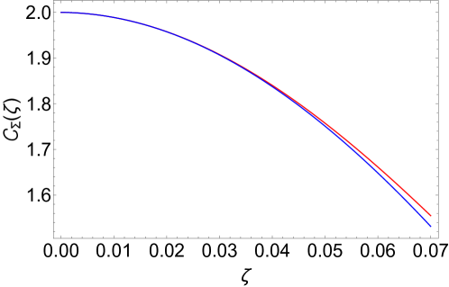
Figure 1: Comparison between the iteration solution of Eq. (100) and the solution of the full differential equation (97) near the UV boundary $\zeta\sim 0$.

The UV boundary conditions given by Eqs. (88)–(90) result in

$$\mathit{x}_{\text{id}}=-\Lambda\frac{2\mathit{x}_{0}\left(4\mathit{y}_{0}^{2}-\mathit{z}_{0}\right)}{\alpha a_{0}\mathit{x}_{0}^{2}-8\mathit{y}_{0}^{2}+2\mathit{z}_{0}},~{}~{}~{}~{}~{}\mathit{y}_{\text{id}}=\Lambda\frac{a_{0}\mathit{x}_{0}}{\alpha a_{0}\mathit{x}_{0}^{2}-8\mathit{y}_{0}^{2}+2\mathit{z}_{0}},~{}~{}~{}~{}~{}\mathit{z}_{\text{id}}=-\Lambda\frac{4a_{0}\mathit{x}_{0}\mathit{y}_{0}}{\alpha a_{0}\mathit{x}_{0}^{2}-8\mathit{y}_{0}^{2}+2\mathit{z}_{0}}.$$

Introducing these results into Eqs. (105)–(107), we obtain the UV solution as

$$X_{uv}(\zeta)=\mathit{x}_{0}-F_{0}\log\left(F_{2}\sinh\left(\zeta F_{1}\Lambda\right)+\cosh\left(\zeta F_{1}\Lambda\right)\right),$$ (111)

$$Y_{uv}(\zeta)=\mathit{y}_{0}-\Lambda F_{3}\zeta-F_{4}\log\left(\cosh\left(\zeta F_{5}\Lambda\right)-F_{6}\sinh\left(\zeta F_{5}\Lambda\right)\right),$$ (112)

$$Z_{uv}(\zeta)=\mathit{z}_{0}+F_{7}\Lambda\zeta-F_{8}\left(1-e^{\zeta F_{9}\Lambda}\right),$$ (113)

where all coefficients are given by

$$F_{0}=\frac{\mathit{x}_{0}\left(\alpha a_{0}\mathit{x}_{0}^{2}-8\mathit{y}_{0}^{2}+2\mathit{z}_{0}\right)}{2\left(\mathit{z}_{0}-4\mathit{y}_{0}^{2}\right)},~{}~{}~{}F_{1}=\frac{2\sqrt{\mathit{x}_{0}^{2}\left(\mathit{z}_{0}-4\mathit{y}_{0}^{2}\right)\left(\frac{6\alpha a_{0}^{2}\mathit{x}_{0}^{3}\mathit{y}_{0}}{\left(\alpha a_{0}\mathit{x}_{0}^{2}-8\mathit{y}_{0}^{2}+2\mathit{z}_{0}\right)^{2}}-4\mathit{y}_{0}^{2}+\mathit{z}_{0}\right)}}{\mathit{x}_{0}\left(\alpha a_{0}\mathit{x}_{0}^{2}-8\mathit{y}_{0}^{2}+2\mathit{z}_{0}\right)},~{}~{}~{}F_{2}=\frac{\left(2\mathit{x}_{0}\left(4\mathit{y}_{0}^{2}-\mathit{z}_{0}\right)\right)\sqrt{\frac{\mathit{z}_{0}-4\mathit{y}_{0}^{2}}{\mathit{x}_{0}^{2}\left(\frac{6\alpha a_{0}^{2}\mathit{x}_{0}^{3}\mathit{y}_{0}}{\left(\alpha a_{0}\mathit{x}_{0}^{2}-8\mathit{y}_{0}^{2}+2\mathit{z}_{0}\right)^{2}}-4\mathit{y}_{0}^{2}+\mathit{z}_{0}\right)}}}{\alpha a_{0}\mathit{x}_{0}^{2}-8\mathit{y}_{0}^{2}+2\mathit{z}_{0}},$$

$$F_{3}=\frac{a_{0}\mathit{x}_{0}}{\alpha a_{0}\mathit{x}_{0}^{2}-8\mathit{y}_{0}^{2}+2\mathit{z}_{0}},~{}~{}~{}F_{4}=\frac{\alpha a_{0}\mathit{x}_{0}^{2}-8\mathit{y}_{0}^{2}+2\mathit{z}_{0}}{4\mathit{y}_{0}},~{}~{}~{}F_{5}=\frac{2\sqrt{a_{0}^{2}\mathit{x}_{0}^{2}\mathit{y}_{0}\left(\alpha^{2}a_{0}\mathit{x}_{0}^{3}+4\left(-4\alpha\mathit{x}_{0}\mathit{y}_{0}^{2}+\alpha\mathit{x}_{0}\mathit{z}_{0}+\mathit{y}_{0}\right)\right)}}{\left(\alpha a_{0}\mathit{x}_{0}^{2}-8\mathit{y}_{0}^{2}+2\mathit{z}_{0}\right)^{2}},$$

$$F_{6}=4a_{0}\mathit{x}_{0}\mathit{y}_{0}\sqrt{\frac{1}{a_{0}^{2}\mathit{x}_{0}^{2}\mathit{y}_{0}\left(\alpha^{2}a_{0}\mathit{x}_{0}^{3}+4\left(-4\alpha\mathit{x}_{0}\mathit{y}_{0}^{2}+\alpha\mathit{x}_{0}\mathit{z}_{0}+\mathit{y}_{0}\right)\right)}},~{}~{}~{}F_{7}=\frac{a_{0}\mathit{x}_{0}\left(\alpha a_{0}\mathit{x}_{0}^{2}\left(2\alpha\mathit{x}_{0}\mathit{y}_{0}-1\right)-2\left(4\alpha\mathit{x}_{0}\mathit{y}_{0}\left(4\mathit{y}_{0}^{2}-\mathit{z}_{0}\right)+\mathit{z}_{0}\right)\right)}{4\mathit{y}_{0}\left(-\alpha a_{0}\mathit{x}_{0}^{2}+8\mathit{y}_{0}^{2}-2\mathit{z}_{0}\right)},$$

$$F_{8}=\frac{\left(-\alpha a_{0}\mathit{x}_{0}^{2}+8\mathit{y}_{0}^{2}-2\mathit{z}_{0}\right)\left(\alpha a_{0}\mathit{x}_{0}^{2}\left(1-2\alpha\mathit{x}_{0}\mathit{y}_{0}\right)+2\left(16\alpha\mathit{x}_{0}\mathit{y}_{0}^{3}-4\alpha\mathit{x}_{0}\mathit{y}_{0}\mathit{z}_{0}+8\mathit{y}_{0}^{2}+\mathit{z}_{0}\right)\right)}{32\mathit{y}_{0}^{2}},~{}~{}~{}F_{9}=\frac{8a_{0}\mathit{x}_{0}\mathit{y}_{0}}{\left(\alpha a_{0}\mathit{x}_{0}^{2}-8\mathit{y}_{0}^{2}+2\mathit{z}_{0}\right)^{2}}.$$

The IR boundary conditions given by Eqs. (85)–(87) result in

$$\mathit{x}_{\text{fd}} = \Lambda\frac{\mathit{x}_{f}\left(4\mathit{y}_{f}^{2}-\mathit{z}_{f}\right)\left(a_{0}\mathit{x}_{f}\left(16\alpha\mathit{x}_{f}\mathit{y}_{f}^{4}-4\alpha\mathit{x}_{f}\mathit{y}_{f}^{2}\left(\mathit{z}_{f}+3\right)+\alpha\mathit{x}_{f}\mathit{z}_{f}+8\mathit{y}_{f}\left(\mathit{z}_{f}+2\right)-32\mathit{y}_{f}^{3}\right)+2\left(4\mathit{y}_{f}^{2}-\mathit{z}_{f}\right)\left(2\mathit{y}_{f}^{2}\left(\alpha\mathit{x}_{f}\mathit{y}_{f}-4\right)+\mathit{z}_{f}\left(2-\alpha\mathit{x}_{f}\mathit{y}_{f}\right)\right)\right)}{\left(2a_{0}\mathit{x}_{f}\mathit{y}_{f}\left(4\mathit{y}_{f}^{2}-\mathit{z}_{f}-2\right)+\left(\mathit{z}_{f}-4\mathit{y}_{f}^{2}\right)^{2}\right)\left(\alpha a_{0}\mathit{x}_{f}^{2}-8\mathit{y}_{f}^{2}+2\mathit{z}_{f}\right)},$$

$$\mathit{y}_{\text{fd}} = \Lambda\frac{-2a_{0}^{2}\mathit{x}_{f}^{2}\mathit{y}_{f}\left(4\mathit{y}_{f}^{2}-\mathit{z}_{f}-2\right)\left(\alpha\mathit{x}_{f}\mathit{y}_{f}-2\right)-a_{0}\mathit{x}_{f}\left(\mathit{z}_{f}-4\mathit{y}_{f}^{2}\right)^{2}\left(\alpha\mathit{x}_{f}\mathit{y}_{f}-3\right)+4\mathit{y}_{f}^{3}\left(\mathit{z}_{f}-4\mathit{y}_{f}^{2}\right)^{2}}{\left(2a_{0}\mathit{x}_{f}\mathit{y}_{f}\left(4\mathit{y}_{f}^{2}-\mathit{z}_{f}-2\right)+\left(\mathit{z}_{f}-4\mathit{y}_{f}^{2}\right)^{2}\right)\left(\alpha a_{0}\mathit{x}_{f}^{2}-8\mathit{y}_{f}^{2}+2\mathit{z}_{f}\right)},$$

$$\mathit{z}_{\text{fd}} = \Lambda\frac{a_{0}A\mathit{x}_{f}\left(4\mathit{y}_{f}^{2}-\mathit{z}_{f}\right)+2a_{0}^{2}B\mathit{x}_{f}^{2}+\alpha a_{0}^{3}\mathit{x}_{f}^{4}\left(4\mathit{y}_{f}^{2}-\mathit{z}_{f}\right)+2\mathit{z}_{f}\left(2\mathit{y}_{f}^{2}-\mathit{z}_{f}\right)\left(\mathit{z}_{f}-4\mathit{y}_{f}^{2}\right){}^{2}}{\left(2a_{0}\mathit{x}_{f}\mathit{y}_{f}\left(4\mathit{y}_{f}^{2}-\mathit{z}_{f}-2\right)+\left(\mathit{z}_{f}-4\mathit{y}_{f}^{2}\right){}^{2}\right)\left(\alpha a_{0}\mathit{x}_{f}^{2}-8\mathit{y}_{f}^{2}+2\mathit{z}_{f}\right)},$$

where $A=8\mathit{y}_{f}^{3}\left(\alpha\mathit{x}_{f}\mathit{y}_{f}-8\right)+2\mathit{y}_{f}\mathit{z}_{f}\left(-3\alpha\mathit{x}_{f}\mathit{y}_{f}+8\mathit{y}_{f}^{2}+2\right)+\mathit{z}_{f}^{2}\left(\alpha\mathit{x}_{f}-4\mathit{y}_{f}\right)$ and $B=16\alpha\mathit{x}_{f}\mathit{y}_{f}^{5}-4\alpha\mathit{x}_{f}\mathit{y}_{f}^{3}\left(2\mathit{z}_{f}+1\right)+\alpha\mathit{x}_{f}\mathit{y}_{f}\mathit{z}_{f}\left(\mathit{z}_{f}+2\right)+16\mathit{y}_{f}^{2}\left(\mathit{z}_{f}+1\right)-48\mathit{y}_{f}^{4}-\mathit{z}_{f}^{2}$. Introducing these results into Eqs. (108)–(110), we obtain the IR solution as the UV one, not shown here.

To solve these three coupled nonlinear second-order differential equations, we consider the matching method as follows:

1. $X(\zeta)$, $Y(\zeta)$, and $Z(\zeta)$: We say $X(\zeta)$ ($Y(\zeta)$ and $Z(\zeta)$) near UV boundary as $X_{uv}(\zeta)$ ($Y_{uv}(\zeta)$ and $Z_{uv}(\zeta)$) and $X(\zeta)$ ($Y(\zeta)$ and $Z(\zeta)$) near IR boundary as $X_{ir}(\zeta)$ ($Y_{ir}(\zeta)$ and $Z_{ir}(\zeta)$). Then, we consider the matching condition at $x_{1}$ ($x_{2}$ and $x_{3}$), given by (1) $X_{uv}(x_{1})=X_{ir}(x_{1})$ ($Y_{uv}(x_{2})=Y_{ir}(x_{2})$ and $Z_{uv}(x_{3})=Z_{ir}(x_{3})$), (2) $\partial_{\zeta}X_{uv}(\zeta)\Big{|}_{\zeta=x_{1}}=\partial_{\zeta}X_{ir}(\zeta)\Big{|}_{\zeta=x_{1}}$ ($\partial_{\zeta}Y_{uv}(\zeta)\Big{|}_{\zeta=x_{2}}=\partial_{\zeta}Y_{ir}(\zeta)\Big{|}_{\zeta=x_{2}}$ and $\partial_{\zeta}Z_{uv}(\zeta)\Big{|}_{\zeta=x_{3}}=\partial_{\zeta}Z_{ir}(\zeta)\Big{|}_{\zeta=x_{3}}$), and (3) $\partial_{\zeta}^{2}X_{uv}(\zeta)\Big{|}_{\zeta=x_{1}}=\partial_{\zeta}^{2}X_{ir}(\zeta)\Big{|}_{\zeta=x_{1}}$ ($\partial_{\zeta}^{2}Y_{uv}(\zeta)\Big{|}_{\zeta=x_{2}}=\partial_{\zeta}^{2}Y_{ir}(\zeta)\Big{|}_{\zeta=x_{2}}$ and $\partial_{\zeta}^{2}Z_{uv}(\zeta)\Big{|}_{\zeta=x_{3}}=\partial_{\zeta}^{2}Z_{ir}(\zeta)\Big{|}_{\zeta=x_{3}}$).

2. Solving these three equations, we obtain $x_{1}$ ($x_{2}$ and $x_{3}$) and determine $x_{0}$ ($y_{0}$ and $z_{0}$) and $x_{f}$ ($y_{f}$ and $z_{f}$) in a self-consistent way.

3. In general, we find that the matching point occurs near either UV or IR boundary. Counting the power of $\Lambda$ in the four constrained conditions, $\partial_{\zeta}X_{uv}(\zeta)\Big{|}_{\zeta=x_{1}}=\partial_{\zeta}X_{ir}(\zeta)\Big{|}_{\zeta=x_{1}}$ and $\partial_{\zeta}^{2}X_{uv}(\zeta)\Big{|}_{\zeta=x_{1}}=\partial_{\zeta}^{2}X_{ir}(\zeta)\Big{|}_{\zeta=x_{1}}$ ($\partial_{\zeta}Y_{uv}(\zeta)\Big{|}_{\zeta=x_{2}}=\partial_{\zeta}Y_{ir}(\zeta)\Big{|}_{\zeta=x_{2}}$ and $\partial_{\zeta}^{2}Y_{uv}(\zeta)\Big{|}_{\zeta=x_{2}}=\partial_{\zeta}^{2}Y_{ir}(\zeta)\Big{|}_{\zeta=x_{2}}$), we obtain $\sim(z_{f}-4y_{f}^{2})\Lambda^{3}$ in the leading order and $\sim(z_{0}-4y_{0}^{2})\Lambda^{2}$ in the subleading one. As a result, we find $z_{0}=4y_{0}^{2}$ and $z_{f}=4y_{f}^{2}$. These equations simplify the procedure significantly.

4. After tedious and lengthy calculations, the three matching points are given by $x_{1}=\frac{\gamma_{1}}{\Lambda}+\frac{\gamma_{2}}{\Lambda^{2}}$, $x_{2}=\frac{\gamma_{3}}{\Lambda^{3/2}}$, and $x_{3}=1-\frac{\gamma_{4}}{\Lambda}-\frac{\gamma_{5}}{\Lambda^{2}}$, respectively. Here, we obtain $\gamma_{i}\sim\mathcal{O}(1)$ to be specified below.

Taking into account $z_{0}=4y_{0}^{2}$ and $z_{f}=4y_{f}^{2}$, we simplify both UV and IR solutions (Eqs. (108)–(110) & Eqs. (111)–(113)). The UV solution is

$$X_{uv}(\zeta)=\mathit{x}_{0}-\frac{6\Lambda^{2}\mathit{y}_{0}}{\alpha^{2}a_{0}\mathit{x}_{0}^{2}}\zeta^{2},$$ (114)

$$Y_{uv}(\zeta)=\mathit{y}_{0}-\frac{\zeta\Lambda}{\alpha\mathit{x}_{0}}-\frac{\alpha a_{0}\mathit{x}_{0}^{2}}{4\mathit{y}_{0}}\log(\cosh(\zeta T)-R\sinh(\zeta T)),$$ (115)

$$Z_{uv}(\zeta)=\frac{\alpha a_{0}\mathit{x}_{0}^{2}\left(24\mathit{y}_{0}^{2}-\alpha a_{0}\mathit{x}_{0}^{2}\left(2\alpha\mathit{x}_{0}\mathit{y}_{0}-1\right)\right)}{32\mathit{y}_{0}^{2}}\left(1-e^{\frac{8\zeta\Lambda\mathit{y}_{0}}{\alpha^{2}a_{0}\mathit{x}_{0}^{3}}}\right)+\frac{a_{0}\zeta\Lambda\mathit{x}_{0}\left(1-2\alpha\mathit{x}_{0}\mathit{y}_{0}\right)}{4\mathit{y}_{0}}+\frac{2\zeta\Lambda\mathit{y}_{0}}{\alpha\mathit{x}_{0}}+4\mathit{y}_{0}^{2},$$ (116)

where

$$T=\frac{2\Lambda\sqrt{a_{0}^{2}\mathit{x}_{0}^{2}\mathit{y}_{0}\left(\alpha^{2}a_{0}\mathit{x}_{0}^{3}+4\mathit{y}_{0}\right)}}{\alpha^{2}a_{0}^{2}\mathit{x}_{0}^{4}},~{}~{}~{}~{}~{}R=4a_{0}\mathit{x}_{0}\mathit{y}_{0}\sqrt{\frac{1}{\alpha^{2}a_{0}^{3}\mathit{x}_{0}^{5}\mathit{y}_{0}+4a_{0}^{2}\mathit{x}_{0}^{2}\mathit{y}_{0}^{2}}}.$$

The IR solution is

$$X_{ir}(\zeta)\approx\frac{12\mathit{y}_{f}\left(\alpha\Lambda\mathfrak{X}_{d}\mathit{y}_{f}-2\right)}{\alpha^{2}a_{0}\mathfrak{X}_{d}^{2}}(1-\zeta)^{2}+\Lambda\mathfrak{X}_{d},$$ (117)

$$Y_{ir}(\zeta)\approx\mathit{y}_{f}+\frac{\alpha\Lambda\mathfrak{X}_{d}\mathit{y}_{f}+4}{2\alpha\mathfrak{X}_{d}}(1-\zeta)-\frac{\alpha a_{0}\Lambda^{2}\mathfrak{X}_{d}^{2}}{4\mathit{y}_{f}}\log(\cosh((1-\zeta)V)-W\sinh((1-\zeta)V)),$$ (118)

$$Z_{ir}(\zeta)\approx G\left(1-\exp\left(\frac{8\mathit{y}_{f}\left(\alpha\Lambda\mathfrak{X}_{d}\mathit{y}_{f}-2\right)}{\alpha^{2}a_{0}\Lambda^{2}\mathfrak{X}_{d}^{3}}(1-\zeta)\right)\right)+4\mathit{y}_{f}^{2}+(1-\zeta)Q.$$ (119)

Here, we introduced $\mathit{x}_{f}=\Lambda\mathfrak{X}_{d}$ for convenience. In these expressions, $V$, $W$, $Q$, and $G$ are given by

$$V = 2\sqrt{\frac{\mathit{y}_{f}\left(\alpha^{2}a_{0}\Lambda^{3}\mathfrak{X}_{d}^{3}+\alpha^{2}\Lambda^{2}\mathfrak{X}_{d}^{2}\mathit{y}_{f}^{3}+8\alpha\Lambda\mathfrak{X}_{d}\mathit{y}_{f}^{2}+16\mathit{y}_{f}\right)}{\alpha^{4}a_{0}^{2}\Lambda^{4}\mathfrak{X}_{d}^{6}}},~{}~{}~{}~{}~{}W=\frac{\mathit{y}_{f}\left(\alpha\Lambda\mathfrak{X}_{d}\mathit{y}_{f}-8\right)\sqrt{\frac{\alpha^{4}a_{0}^{2}\Lambda^{4}\mathfrak{X}_{d}^{6}}{\alpha^{2}a_{0}\Lambda^{3}\mathfrak{X}_{d}^{3}\mathit{y}_{f}+4\alpha^{2}\Lambda^{2}\mathfrak{X}_{d}^{2}\mathit{y}_{f}^{4}+32\alpha\Lambda\mathfrak{X}_{d}\mathit{y}_{f}^{3}+64\mathit{y}_{f}^{2}}}}{\alpha^{2}a_{0}\Lambda^{2}\mathfrak{X}_{d}^{3}},$$

$$Q = \frac{a_{0}\Lambda^{2}\mathfrak{X}_{d}\left(\alpha\Lambda\mathfrak{X}_{d}\mathit{y}_{f}\left(\alpha\Lambda\mathfrak{X}_{d}\mathit{y}_{f}-6\right)+4\right)}{4\mathit{y}_{f}\left(\alpha\Lambda\mathfrak{X}_{d}\mathit{y}_{f}-2\right)}+2\mathit{y}_{f}\left(\Lambda\mathit{y}_{f}-\frac{2}{\alpha\mathfrak{X}_{d}}\right),~{}~{}~{}~{}~{}G=\frac{\alpha a_{0}\Lambda^{2}\mathfrak{X}_{d}^{2}\left(\frac{\alpha a_{0}\Lambda^{2}\mathfrak{X}_{d}^{2}\left(\alpha\Lambda\mathfrak{X}_{d}\mathit{y}_{f}\left(\alpha\Lambda\mathfrak{X}_{d}\mathit{y}_{f}-6\right)+4\right)}{\mathit{y}_{f}^{2}}-48\alpha\Lambda\mathfrak{X}_{d}\mathit{y}_{f}+96\right)}{32\left(\alpha\Lambda\mathfrak{X}_{d}\mathit{y}_{f}-2\right)^{2}},$$

respectively.

After lengthy but straightforward computations at sufficiently large $\Lambda$, we obtain the UV solution

$$\mathit{x}_{0}=x_{p}+\frac{\epsilon_{0}}{\Lambda},~{}~{}~{}~{}~{}\mathit{y}_{0}=\frac{1}{8}\left(\sqrt{\alpha^{4}a_{0}^{2}x_{0}^{6}-8\alpha a_{0}x_{0}^{2}}+\alpha^{2}a_{0}x_{0}^{3}\right),~{}~{}~{}~{}~{}\mathit{z}_{0}=4\mathit{y}_{0}^{2},$$ (120)

$$x_{p}=\frac{2\sqrt[4]{3}}{\alpha^{3/4}\sqrt[4]{-a_{0}}}-\frac{\sqrt{41722\sqrt{42}+484599}}{4\sqrt{\Lambda}3^{3/4}\sqrt{34}\alpha^{3/4}\sqrt[4]{-a_{0}}},$$ (121)

$$\epsilon_{0}=\frac{3\alpha^{13/2}a_{0}^{3}x_{0}^{9}+10\sqrt{3}\sqrt{-a_{0}}\sqrt{\alpha a_{0}x_{0}^{2}\left(\alpha^{3}a_{0}x_{0}^{4}-8\right)}+20\sqrt{3}\alpha^{2}\left(-a_{0}\right)^{3/2}x_{0}^{3}+3\alpha^{7/2}a_{0}^{2}x_{0}^{5}\left(\alpha x_{0}\sqrt{\alpha a_{0}x_{0}^{2}\left(\alpha^{3}a_{0}x_{0}^{4}-8\right)}+8\right)}{12\sqrt{\alpha}a_{0}\left(3\alpha^{3}a_{0}x_{0}^{4}+8\right)},$$ (122)

and the IR solution

$$\mathit{x}_{f}=\Lambda\mathfrak{X}_{d},~{}~{}~{}~{}~{}\mathit{z}_{f}=4\mathit{y}_{f}^{2},~{}~{}~{}~{}~{}\mathit{y}_{f}=\frac{\sqrt[4]{-a_{0}}}{2\sqrt[4]{3}\sqrt[4]{\alpha}}+\frac{\delta_{1}}{\Lambda},$$ (123)

$$\mathfrak{X}_{d}=\frac{\sqrt{-a_{0}}\left(-12\alpha^{4}\mathit{x}_{0}^{4}\mathit{y}_{f}^{6}+4\alpha^{2}\mathit{x}_{0}^{2}\mathit{y}_{0}\mathit{y}_{f}^{3}\left(\alpha\mathit{x}_{0}\mathit{y}_{f}-6\right)+\mathit{y}_{0}^{2}\left(\alpha^{2}\mathit{x}_{0}^{2}\mathit{y}_{f}^{2}+4\alpha\mathit{x}_{0}\mathit{y}_{f}-12\right)\right)}{\Lambda^{2}\left(16\sqrt{3}\alpha^{3/2}\mathit{y}_{0}^{2}\mathit{y}_{f}^{3}\right)}+\frac{2\sqrt{3}\mathit{y}_{f}}{\sqrt{\alpha}\sqrt{-a_{0}}}+\frac{-\frac{\alpha\mathit{x}_{0}^{2}\mathit{y}_{f}^{2}}{\mathit{y}_{0}}-\frac{1}{\alpha\mathit{y}_{f}}+\frac{\mathit{x}_{0}}{2}}{\Lambda},$$ (124)

$$\delta_{1}=\frac{a_{0}\left(18\alpha^{2}\sqrt{-a_{0}}x_{0}^{2}y_{f}^{3}-9\alpha\sqrt{-a_{0}}x_{0}\mathit{y}_{0}y_{f}+\mathit{y}_{0}\left(19\sqrt{-a_{0}}+140\sqrt{3}\sqrt{\alpha}y_{f}^{2}\right)\right)+54\alpha\mathit{y}_{0}y_{f}^{3}\left(8\sqrt{-a_{0}}y_{f}-8\sqrt{-a_{0}}\mathit{y}_{0}+\sqrt{3}\sqrt{\alpha}y_{f}^{3}\right)}{36\left(\sqrt{3}\sqrt{\alpha}a_{0}\mathit{y}_{0}y_{f}-12\alpha\sqrt{-a_{0}}\mathit{y}_{0}y_{f}^{3}\right)},$$ (125)

respectively. These two solutions meet at

$$x_{1}=\frac{\gamma_{1}}{\Lambda}+\frac{\gamma_{2}}{\Lambda^{2}},~{}~{}~{}~{}~{}x_{2}=\frac{\gamma_{3}}{\Lambda^{3/2}},~{}~{}~{}~{}~{}x_{3}=1-\frac{\gamma_{4}}{\Lambda}-\frac{\gamma_{5}}{\Lambda^{2}},$$

$$\gamma_{1}=\frac{2\alpha\mathit{x}_{0}^{2}\mathit{y}_{f}^{2}}{\mathit{y}_{0}\mathfrak{X}_{d}},~{}~{}~{}~{}~{}\gamma_{2}=-\frac{4\left(\alpha^{2}\mathit{x}_{0}^{4}\mathit{y}_{f}^{4}+\mathit{x}_{0}^{2}\mathit{y}_{0}\mathit{y}_{f}\right)}{\mathit{y}_{0}^{2}\mathfrak{X}_{d}^{2}},~{}~{}~{}~{}~{}\gamma_{3}=-\frac{a_{0}\alpha^{2}x_{0}^{7/2}}{24}\sqrt{\frac{6a_{0}ky_{f}^{2}-81\sqrt{\alpha}\sqrt{-a_{0}}\mathit{y}_{0}y_{f}^{5}\left(\alpha x_{0}^{2}\left(33y_{f}-32\mathit{y}_{0}\right)+32\epsilon_{0}\right)-\sqrt{3}a_{0}^{2}x_{0}^{2}\mathit{y}_{0}}{x_{0}^{2}\mathit{y}_{0}^{2}y_{f}^{3}\left(12\sqrt{\alpha}\sqrt{-a_{0}}y_{f}^{2}-\sqrt{3}a_{0}\right)\left(3\alpha^{2}a_{0}x_{0}^{3}-36\mathit{y}_{0}\right)}},$$

(129)

$$\gamma_{4}=1,~{}~{}~{}~{}~{}\gamma_{5}=20-\frac{\sqrt{3}\epsilon_{0}\left(\sqrt{\alpha a_{0}x_{0}^{2}\left(\alpha^{3}a_{0}x_{0}^{4}-8\right)}+2\alpha^{2}a_{0}x_{0}^{3}\right)}{\sqrt{\alpha}\sqrt{-a_{0}}x_{0}^{2}},$$

$$k=18\sqrt{-a_{0}}\alpha^{5/2}x_{0}^{4}y_{f}^{3}-9\sqrt{-a_{0}}\alpha^{3/2}x_{0}^{3}\mathit{y}_{0}y_{f}-16\sqrt{\alpha}\sqrt{-a_{0}}x_{0}^{2}\mathit{y}_{0}+4\sqrt{3}\mathit{y}_{0}y_{f}\left(2\alpha x_{0}^{2}\left(8y_{f}-9\mathit{y}_{0}\right)+9\epsilon_{0}\right).$$

Finally, we are ready to discuss the RG flows of $\mathcal{C}_{\Sigma}(\zeta)$, $\mathcal{C}_{G}(\zeta)$, and $\mathcal{C}_{\Pi}(\zeta)$. The blue curve in Fig. 2 (b) is a plot of the UV solution Eq. (115) while the red one is a plot of the IR solution Eq. (117). The matching point is obtained by Eq. (III.2), which occurs near the UV boundary. Similarly, the RG flow of $\mathcal{C}_{G}(\zeta)$ is given in Fig. 3, where the matching point is realized near the UV boundary. The RG flow of $\mathcal{C}_{\Pi}(\zeta)$ is given in Fig. 4. In this case, the matching point appears near the IR boundary. It is quite interesting to observe $\mathcal{C}_{\Sigma}(1)\sim\mathcal{O}(\Lambda)$ while $\mathcal{C}_{G}(1)\sim\mathcal{O}(1)$ and $\mathcal{C}_{\Pi}(1)\sim\mathcal{O}(1)$. In other words, the renormalized self-energy diverges at IR, which indicates that the conformal solution becomes unstable and an excitation gap is formed. As a result, we obtain an insulating behavior, which will be more clarified in the density of states below.

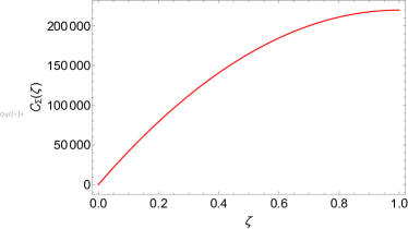
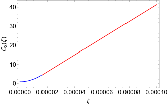
Figure 2: RG flow of $\mathcal{C}_{\Sigma}(\zeta)$. (a) $\mathcal{C}_{\Sigma}(\zeta)$ vs. $\zeta$ overall. (b) $\mathcal{C}_{\Sigma}(\zeta)$ vs. $\zeta$ zoomed near UV. Here, we set $a_{0}=-0.01$, $\Lambda=500000$, and $\alpha=20$.

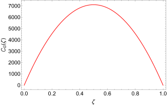
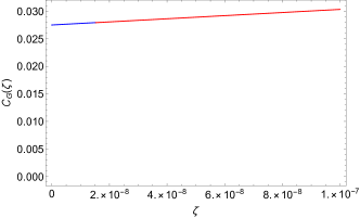
Figure 3: RG flow of $\mathcal{C}_{G}(\zeta)$. (a) $\mathcal{C}_{G}(\zeta)$ vs. $\zeta$ overall. (b) $\mathcal{C}_{G}(\zeta)$ vs. $\zeta$ zoomed near UV. Here, we set $a_{0}=-0.01$, $\Lambda=500000$, and $\alpha=20$.

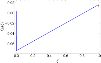
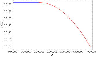
Figure 4: RG flow of $\mathcal{C}_{\Pi}(\zeta)$. (a) $\mathcal{C}_{\Pi}(\zeta)$ vs. $\zeta$ overall. (b) $\mathcal{C}_{\Pi}(\zeta)$ vs. $\zeta$ zoomed near IR. Here, we set $a_{0}=-0.01$, $\Lambda=500000$, and $\alpha=20$.

III.3 Thermodynamics

To verify the holographic dual effective field theory for an SYK model, we investigate thermodynamics. In particular, we show that the finite density of states due to the finite residual entropy in the field theoretic large $N$ limit vanishes in the large $N$ limit of the holographic dual effective field theory.

It is straightforward to generalize the conformal ansatz at zero temperature to that at finite temperatures, given by [39, 40, 41, 42, 43]

$$\Sigma(\tau^{\prime}-\tau,z)=\mathcal{C}_{\Sigma}(z)\mbox{sgn}(\tau-\tau^{\prime})\Big{|}\frac{\pi\beta^{-1}}{\sin[\pi\beta^{-1}(\tau-\tau^{\prime})]}\Big{|}^{\Delta_{\Sigma}},$$

$$G(\tau^{\prime}-\tau,z)=\mathcal{C}_{G}(z)\mbox{sgn}(\tau-\tau^{\prime})\Big{|}\frac{\pi\beta^{-1}}{\sin[\pi\beta^{-1}(\tau-\tau^{\prime})]}\Big{|}^{\Delta_{G}},$$

$$\Pi(\tau^{\prime}-\tau,z)=\mathcal{C}_{\Pi}(z)\Big{|}\frac{\pi\beta^{-1}}{\sin[\pi\beta^{-1}(\tau-\tau^{\prime})]}\Big{|}^{\Delta_{\Pi}}.$$ (130)

Inserting this finite-temperature ansatz into Eqs. (26), (27), and (28), we obtain the same differential equations (94), (95), and (96) for the RG flows of $\mathcal{C}_{\Sigma}(z)$, $\mathcal{C}_{G}(z)$, and $\mathcal{C}_{\Pi}(z)$ and the same UV and IR boundary conditions as those at zero temperature, where the conformal dimensions of $\Delta_{\Sigma}=\frac{3}{2}$, $\Delta_{G}=\frac{1}{2}$, and $\Delta_{\Pi}=1$ remain unchanged. In appendix B, we confirm this statement based on our explicit calculations.

To find the free energy, we perform the Fourier transformations for all the collective bi-local fields as follows

$$\Sigma(i\omega_{n},z)=\int_{0}^{\beta}d\tau e^{i\omega_{n}\tau}\Sigma(\tau,z)=\mbox{sgn}(\omega_{n})F(i\omega_{n};\beta,\Delta_{\Sigma})\mathcal{C}_{\Sigma}(z),$$ (131)

$$G(i\omega_{n},z)=\int_{0}^{\beta}d\tau e^{i\omega_{n}\tau}G(\tau,z)=\mbox{sgn}(\omega_{n})F(i\omega_{n};\beta,\Delta_{G})\mathcal{C}_{G}(z),$$ (132)

$$\Pi(i\omega_{n},z)=\int_{0}^{\beta}d\tau e^{i\omega_{n}\tau}\Pi(\tau,z)=\tilde{F}(i\omega_{n};\beta,\Delta_{\Pi})\mathcal{C}_{\Pi}(z),$$ (133)

where

$$F(i\omega_{n};\beta,y)=\int_{0}^{\beta}d\tau e^{i\omega_{n}\tau}\mbox{sgn}(\omega_{n}\tau)\Big{|}\frac{\pi\beta^{-1}}{\sin[\pi\beta^{-1}\tau]}\Big{|}^{y},$$ (134)

$$\tilde{F}(i\omega_{n};\beta,y)=\int_{0}^{\beta}d\tau e^{i\omega_{n}\tau}\Big{|}\frac{\pi\beta^{-1}}{\sin[\pi\beta^{-1}\tau]}\Big{|}^{y}.$$ (135)

Here, $\omega_{n}=(2n+1)\pi/\beta$ ($\omega_{n}=2n\pi/\beta$) is the fermionic (bosonic) Matsubara frequency with integer $n$.

Introducing these Fourier-transformed representations into Eq. (9), we obtain

$$\mathcal{Z}_{SYK}=\int D\mathcal{C}_{\Sigma}(z)D\mathcal{C}_{\Pi}(z)D\mathcal{C}_{G}(z)\exp\Big{[}-N\sum_{i\omega_{n}}\Big{\{}-\frac{1}{2}\ln\Big{(}q_{d}\Gamma_{J}\mbox{sgn}(\omega_{n})F(i\omega_{n};\beta,\Delta_{\Sigma})\mathcal{C}_{\Sigma}(z_{f})\Big{)}$$

$$-q_{d}\Gamma_{J}F(i\omega_{n};\beta,\Delta_{\Sigma})F(i\omega_{n};\beta,\Delta_{G})\mathcal{C}_{\Sigma}(z_{f})\mathcal{C}_{G}(z_{f})+q_{d}\Gamma_{J}F(i\omega_{n};\beta,\Delta_{\Pi})F(i\omega_{n};\beta,2\Delta_{G})\mathcal{C}_{\Pi}(0)\mathcal{C}_{G}^{2}(0)+\frac{q_{d}\Gamma_{J}}{4}F^{2}(i\omega_{n};\beta,\Delta_{\Pi})\mathcal{C}_{\Pi}^{2}(0)\Big{\}}$$

$$-N\sum_{i\omega_{n}}\int_{0}^{z_{f}}dz\Big{\{}-\frac{1}{2}[\partial_{z}\ln\mathcal{C}_{\Sigma}(z)]+\frac{1}{4}[\partial_{z}\ln\mathcal{C}_{\Sigma}(z)]^{2}-q_{d}\Gamma_{J}F(i\omega_{n};\beta,\Delta_{\Sigma})F(i\omega_{n};\beta,\Delta_{G})[\partial_{z}\mathcal{C}_{\Sigma}(z)][\partial_{z}\mathcal{C}_{G}(z)]$$

$$+2q_{d}\Gamma_{J}F(i\omega_{n};\beta,\Delta_{\Pi})F(i\omega_{n};\beta,2\Delta_{G})\mathcal{C}_{\Pi}(z)\mathcal{C}_{G}(z)[\partial_{z}\mathcal{C}_{G}(z)]+q_{d}\Gamma_{J}F(i\omega_{n};\beta,\Delta_{\Pi})F(i\omega_{n};\beta,2\Delta_{G})\mathcal{C}_{G}^{2}(z)[\partial_{z}\mathcal{C}_{\Pi}(z)]+\frac{q_{d}\Gamma_{J}}{2}F^{2}(i\omega_{n};\beta,\Delta_{\Pi})\mathcal{C}_{\Pi}(z)[\partial_{z}\mathcal{C}_{\Pi}(z)]$$

$$+2q_{d}\Gamma_{J}F(i\omega_{n};\beta,\Delta_{\Pi})F(i\omega_{n};\beta,2\Delta_{G})[\partial_{z}\mathcal{C}_{\Pi}(z)]\mathcal{C}_{G}(z)[\partial_{z}\mathcal{C}_{G}(z)]+q_{d}\Gamma_{J}F(i\omega_{n};\beta,\Delta_{\Pi})F(i\omega_{n};\beta,2\Delta_{G})\mathcal{C}_{\Pi}(z)[\partial_{z}\mathcal{C}_{G}(z)]^{2}+\frac{q_{d}\Gamma_{J}}{4}F^{2}(i\omega_{n};\beta,\Delta_{\Pi})[\partial_{z}\mathcal{C}_{\Pi}(z)]^{2}$$

$$-\frac{1}{2}\ln\Big{(}q_{d}\Gamma_{J}\mbox{sgn}(\omega_{n})F(i\omega_{n};\beta,\Delta_{\Sigma})\mathcal{C}_{\Sigma}(z)\Big{)}\Big{\}}\Big{]}.$$ (136)

As discussed before, we extremize this effective action to take variations with respect to $\mathcal{C}_{\Sigma}(z)$, $\mathcal{C}_{\Pi}(z)$, and $\mathcal{C}_{G}(z)$. To make the resulting three coupled equations be satisfied, regardless of the frequency, we enforce three constraint equations, which fix the critical exponents. As discussed in appendix B, such critical exponents remain unchanged.

To find the onshell effective action, we derive the Hamiltonian formulation from the above expression as follows

$$\mathcal{Z}_{SYK}=\int D\mathcal{C}_{\Sigma}(z)D\Pi_{\mathcal{C}_{\Sigma}}(z)D\mathcal{C}_{\Pi}(z)D\Pi_{\mathcal{C}_{\Pi}}(z)D\mathcal{C}_{G}(z)D\Pi_{\mathcal{C}_{G}}(z)\exp\Bigg{[}-N\sum_{i\omega_{n}}\Bigg{\{}-\frac{1}{2}\ln\Big{(}q_{d}\Gamma_{J}\mbox{sgn}(\omega_{n})F(i\omega_{n};\beta,\Delta_{\Sigma})\mathcal{C}_{\Sigma}(z_{f})\Big{)}$$

$$-q_{d}\Gamma_{J}F(i\omega_{n};\beta,\Delta_{\Sigma})F(i\omega_{n};\beta,\Delta_{G})\mathcal{C}_{\Sigma}(z_{f})\mathcal{C}_{G}(z_{f})+q_{d}\Gamma_{J}F(i\omega_{n};\beta,\Delta_{\Pi})F(i\omega_{n};\beta,2\Delta_{G})\mathcal{C}_{\Pi}(z_{f})\mathcal{C}_{G}^{2}(z_{f})+\frac{q_{d}\Gamma_{J}}{4}F^{2}(i\omega_{n};\beta,\Delta_{\Pi})\mathcal{C}_{\Pi}^{2}(z_{f})$$

$$-\frac{1}{2}\ln\mathcal{C}_{\Sigma}(z_{f})+\frac{1}{2}\ln\mathcal{C}_{\Sigma}(0)\Bigg{\}}-N\sum_{i\omega_{n}}\int_{0}^{z_{f}}dz\Bigg{\{}\Pi_{\mathcal{C}_{\Sigma}}(z)\partial_{z}\mathcal{C}_{\Sigma}(z)-\Bigg{(}\frac{1}{\mathcal{C}_{\Sigma}^{2}(z)}-\frac{q_{d}\Gamma_{J}\frac{F^{2}(i\omega_{n};\beta,\Delta_{\Sigma})F^{2}(i\omega_{n};\beta,\Delta_{G})}{F(i\omega_{n};\beta,\Delta_{\Pi})F(i\omega_{n};\beta,2\Delta_{G})}}{\mathcal{C}_{\Pi}(z)-4\frac{F(i\omega_{n};\beta,2\Delta_{G})}{F(i\omega_{n};\beta,\Delta_{\Pi})}\mathcal{C}_{G}^{2}(z)}\Bigg{)}^{-1}\Pi_{\mathcal{C}_{\Sigma}}^{2}(z)$$

$$+\Pi_{\mathcal{C}_{G}}(z)\Bigg{(}\partial_{z}\mathcal{C}_{G}(z)-\frac{1}{2}\frac{\frac{F(i\omega_{n};\beta,\Delta_{\Sigma})F(i\omega_{n};\beta,\Delta_{G})}{F(i\omega_{n};\beta,\Delta_{\Pi})F(i\omega_{n};\beta,2\Delta_{G})}}{\mathcal{C}_{\Pi}(z)-4\frac{F(i\omega_{n};\beta,2\Delta_{G})}{F(i\omega_{n};\beta,\Delta_{\Pi})}\mathcal{C}_{G}^{2}(z)}\partial_{z}\mathcal{C}_{\Sigma}(z)\Bigg{)}-\frac{1}{4q_{d}\Gamma_{J}}\frac{\Bigg{(}\mathcal{C}_{\Pi}(z)-4\frac{F(i\omega_{n};\beta,2\Delta_{G})}{F(i\omega_{n};\beta,\Delta_{\Pi})}\mathcal{C}_{G}^{2}(z)\Bigg{)}^{-1}}{F(i\omega_{n};\beta,\Delta_{\Pi})F(i\omega_{n};\beta,2\Delta_{G})}\Pi_{\mathcal{C}_{G}}^{2}(z)$$

$$+\Pi_{\mathcal{C}_{\Pi}}(z)\Bigg{(}\partial_{z}\mathcal{C}_{\Pi}(z)+4\frac{F(i\omega_{n};\beta,2\Delta_{G})}{F(i\omega_{n};\beta,\Delta_{\Pi})}\mathcal{C}_{G}(z)[\partial_{z}\mathcal{C}_{G}(z)]\Bigg{)}-\frac{1}{q_{d}\Gamma_{J}}\frac{1}{F^{2}(i\omega_{n};\beta,\Delta_{\Pi})}\Pi_{\mathcal{C}_{\Pi}(z)}^{2}(z)-\frac{1}{2}\ln\Big{(}q_{d}\Gamma_{J}F(i\omega_{n};\beta,\Delta_{\Sigma})\mathcal{C}_{\Sigma}(z)\Big{)}\Bigg{\}}\Bigg{]}.$$ (137)

Most bulk terms do not contribute to the onshell free energy in the large $N-$limit of this holographic dual effective field theory, where equations of motion are taken into account. As a result, we obtain

$$F_{eff}(\beta)=\frac{N}{\beta}\sum_{i\omega_{n}}\Big{\{}-\frac{1}{2}\ln\Big{(}q_{d}\Gamma_{J}\mbox{sgn}(\omega_{n})F(i\omega_{n};\beta,\Delta_{\Sigma})\mathcal{C}_{\Sigma}(z_{f})\Big{)}-q_{d}\Gamma_{J}F(i\omega_{n};\beta,\Delta_{\Sigma})F(i\omega_{n};\beta,\Delta_{G})\mathcal{C}_{\Sigma}(z_{f})\mathcal{C}_{G}(z_{f})$$

$$+q_{d}\Gamma_{J}F(i\omega_{n};\beta,\Delta_{\Pi})F(i\omega_{n};\beta,2\Delta_{G})\mathcal{C}_{\Pi}(z_{f})\mathcal{C}_{G}^{2}(z_{f})+\frac{q_{d}\Gamma_{J}}{4}F^{2}(i\omega_{n};\beta,\Delta_{\Pi})\mathcal{C}_{\Pi}^{2}(z_{f})-\frac{1}{2}\ln\mathcal{C}_{\Sigma}(z_{f})+\frac{1}{2}\ln\mathcal{C}_{\Sigma}(0)\Big{\}}$$

$$+\frac{N}{\beta}\sum_{i\omega_{n}}\Bigg{\{}\Pi_{\mathcal{C}_{\Sigma}}(z_{f})\mathcal{C}_{\Sigma}(z_{f})+\Pi_{\mathcal{C}_{\Pi}}(z_{f})\Bigg{(}\mathcal{C}_{\Pi}(z_{f})+2\frac{F(i\omega_{n};\beta,2\Delta_{G})}{F(i\omega_{n};\beta,\Delta_{\Pi})}\mathcal{C}_{G}^{2}(z_{f})\Bigg{)}+\Pi_{\mathcal{C}_{G}}(z_{f})\Bigg{(}\mathcal{C}_{G}(z_{f})-\frac{1}{2}\frac{\frac{F(i\omega_{n};\beta,\Delta_{\Sigma})F(i\omega_{n};\beta,\Delta_{G})}{F(i\omega_{n};\beta,\Delta_{\Pi})F(i\omega_{n};\beta,2\Delta_{G})}}{\mathcal{C}_{\Pi}(z_{f})-4\frac{F(i\omega_{n};\beta,2\Delta_{G})}{F(i\omega_{n};\beta,\Delta_{\Pi})}\mathcal{C}_{G}^{2}(z_{f})}\mathcal{C}_{\Sigma}(z_{f})\Bigg{)}$$

$$-\Pi_{\mathcal{C}_{\Sigma}}(0)\mathcal{C}_{\Sigma}(0)-\Pi_{\mathcal{C}_{\Pi}}(0)\Bigg{(}\mathcal{C}_{\Pi}(0)+2\frac{F(i\omega_{n};\beta,2\Delta_{G})}{F(i\omega_{n};\beta,\Delta_{\Pi})}\mathcal{C}_{G}^{2}(0)\Bigg{)}-\Pi_{\mathcal{C}_{G}}(0)\Bigg{(}\mathcal{C}_{G}(0)-\frac{1}{2}\frac{\frac{F(i\omega_{n};\beta,\Delta_{\Sigma})F(i\omega_{n};\beta,\Delta_{G})}{F(i\omega_{n};\beta,\Delta_{\Pi})F(i\omega_{n};\beta,2\Delta_{G})}}{\mathcal{C}_{\Pi}(0)-4\frac{F(i\omega_{n};\beta,2\Delta_{G})}{F(i\omega_{n};\beta,\Delta_{\Pi})}\mathcal{C}_{G}^{2}(0)}\mathcal{C}_{\Sigma}(0)\Bigg{)}\Bigg{\}}.$$ (138)

The three canonical momentums, $\Pi_{\mathcal{C}_{\Sigma}}(z_{f})$, $\Pi_{\mathcal{C}_{\Pi}}(z_{f})$, and $\Pi_{\mathcal{C}_{G}}(z_{f})$ ($\Pi_{\mathcal{C}_{\Sigma}}(0)$, $\Pi_{\mathcal{C}_{\Pi}}(0)$, and $\Pi_{\mathcal{C}_{G}}(0)$) can be represented by their conjugate fields, respectively. Recalling the IR boundary condition,

$$\Pi_{\mathcal{C}_{\Sigma}}(z_{f})=\frac{1}{2}\Bigg{(}\frac{1}{\mathcal{C}_{\Sigma}^{2}(z_{f})}-\frac{q_{d}\Gamma_{J}\frac{F^{2}(i\omega_{n};\beta,\Delta_{\Sigma})F^{2}(i\omega_{n};\beta,\Delta_{G})}{F(i\omega_{n};\beta,\Delta_{\Pi})F(i\omega_{n};\beta,2\Delta_{G})}}{\mathcal{C}_{\Pi}(z_{f})-4\frac{F(i\omega_{n};\beta,2\Delta_{G})}{F(i\omega_{n};\beta,\Delta_{\Pi})}\mathcal{C}_{G}^{2}(z_{f})}\Bigg{)}\partial_{z_{f}}\mathcal{C}_{\Sigma}(z_{f}),$$ (139)

$$\Pi_{\mathcal{C}_{\Pi}}(z_{f})=\frac{q_{d}\Gamma_{J}}{2}F^{2}(i\omega_{n};\beta,\Delta_{\Pi})\Bigg{(}\partial_{z_{f}}\mathcal{C}_{\Pi}(z_{f})+4\frac{F(i\omega_{n};\beta,2\Delta_{G})}{F(i\omega_{n};\beta,\Delta_{\Pi})}\mathcal{C}_{G}(z_{f})[\partial_{z_{f}}\mathcal{C}_{G}(z_{f})]\Bigg{)},$$ (140)

$$\Pi_{\mathcal{C}_{G}}(z_{f})=2q_{d}\Gamma_{J}F(i\omega_{n};\beta,\Delta_{\Pi})F(i\omega_{n};\beta,2\Delta_{G})\Bigg{(}\mathcal{C}_{\Pi}(z_{f})-4\frac{F(i\omega_{n};\beta,2\Delta_{G})}{F(i\omega_{n};\beta,\Delta_{\Pi})}\mathcal{C}_{G}^{2}(z_{f})\Bigg{)}\Bigg{(}\partial_{z_{f}}\mathcal{C}_{G}(z_{f})-\frac{1}{2}\frac{\frac{F(i\omega_{n};\beta,\Delta_{\Sigma})F(i\omega_{n};\beta,\Delta_{G})}{F(i\omega_{n};\beta,\Delta_{\Pi})F(i\omega_{n};\beta,2\Delta_{G})}}{\mathcal{C}_{\Pi}(z_{f})-4\frac{F(i\omega_{n};\beta,2\Delta_{G})}{F(i\omega_{n};\beta,\Delta_{\Pi})}\mathcal{C}_{G}^{2}(z_{f})}\partial_{z_{f}}\mathcal{C}_{\Sigma}(z_{f})\Bigg{)},$$

and the UV one,

$$\Pi_{\mathcal{C}_{\Pi}}(0)=0,~{}~{}~{}~{}~{}\Pi_{\mathcal{C}_{G}}(0)=0,~{}~{}~{}~{}~{}\Pi_{\mathcal{C}_{\Sigma}}(0)=\frac{1}{2}\frac{1}{\mathcal{C}_{\Sigma}(0)},$$ (142)

we obtain the onshell effective free energy functional as follows

$$F_{eff}(\beta)=\frac{N}{\beta}\sum_{i\omega_{n}}\Bigg{\{}-\frac{1}{2}\ln\Big{(}q_{d}\Gamma_{J}\mbox{sgn}(\omega_{n})F(i\omega_{n};\beta,\Delta_{\Sigma})\mathcal{C}_{\Sigma}(z_{f})\Big{)}-q_{d}\Gamma_{J}F(i\omega_{n};\beta,\Delta_{\Sigma})F(i\omega_{n};\beta,\Delta_{G})\mathcal{C}_{\Sigma}(z_{f})\mathcal{C}_{G}(z_{f})$$

$$+q_{d}\Gamma_{J}F(i\omega_{n};\beta,\Delta_{\Pi})F(i\omega_{n};\beta,2\Delta_{G})\mathcal{C}_{\Pi}(z_{f})\mathcal{C}_{G}^{2}(z_{f})+\frac{q_{d}\Gamma_{J}}{4}F^{2}(i\omega_{n};\beta,\Delta_{\Pi})\mathcal{C}_{\Pi}^{2}(z_{f})-\frac{1}{2}\ln\mathcal{C}_{\Sigma}(z_{f})+\frac{1}{2}\ln\mathcal{C}_{\Sigma}(0)\Bigg{\}}$$

$$+\frac{N}{\beta}\sum_{i\omega_{n}}\Bigg{\{}\frac{1}{2}\Bigg{(}\frac{1}{\mathcal{C}_{\Sigma}^{2}(z_{f})}-\frac{q_{d}\Gamma_{J}\frac{F^{2}(i\omega_{n};\beta,\Delta_{\Sigma})F^{2}(i\omega_{n};\beta,\Delta_{G})}{F(i\omega_{n};\beta,\Delta_{\Pi})F(i\omega_{n};\beta,2\Delta_{G})}}{\mathcal{C}_{\Pi}(z_{f})-4\frac{F(i\omega_{n};\beta,2\Delta_{G})}{F(i\omega_{n};\beta,\Delta_{\Pi})}\mathcal{C}_{G}^{2}(z_{f})}\Bigg{)}\mathcal{C}_{\Sigma}(z_{f})\partial_{z_{f}}\mathcal{C}_{\Sigma}(z_{f})$$

$$+\frac{q_{d}\Gamma_{J}}{2}F^{2}(i\omega_{n};\beta,\Delta_{\Pi})\Bigg{(}\mathcal{C}_{\Pi}(z_{f})+2\frac{F(i\omega_{n};\beta,2\Delta_{G})}{F(i\omega_{n};\beta,\Delta_{\Pi})}\mathcal{C}_{G}^{2}(z_{f})\Bigg{)}\Bigg{(}\partial_{z_{f}}\mathcal{C}_{\Pi}(z_{f})+4\frac{F(i\omega_{n};\beta,2\Delta_{G})}{F(i\omega_{n};\beta,\Delta_{\Pi})}\mathcal{C}_{G}(z_{f})[\partial_{z_{f}}\mathcal{C}_{G}(z_{f})]\Bigg{)}$$

$$+2q_{d}\Gamma_{J}F(i\omega_{n};\beta,\Delta_{\Pi})F(i\omega_{n};\beta,2\Delta_{G})\Bigg{(}\mathcal{C}_{\Pi}(z_{f})-4\frac{F(i\omega_{n};\beta,2\Delta_{G})}{F(i\omega_{n};\beta,\Delta_{\Pi})}\mathcal{C}_{G}^{2}(z_{f})\Bigg{)}\Bigg{(}\mathcal{C}_{G}(z_{f})$$

$$-\frac{1}{2}\frac{\frac{F(i\omega_{n};\beta,\Delta_{\Sigma})F(i\omega_{n};\beta,\Delta_{G})}{F(i\omega_{n};\beta,\Delta_{\Pi})F(i\omega_{n};\beta,2\Delta_{G})}}{\mathcal{C}_{\Pi}(z_{f})-4\frac{F(i\omega_{n};\beta,2\Delta_{G})}{F(i\omega_{n};\beta,\Delta_{\Pi})}\mathcal{C}_{G}^{2}(z_{f})}\mathcal{C}_{\Sigma}(z_{f})\Bigg{)}\Bigg{(}\partial_{z_{f}}\mathcal{C}_{G}(z_{f})-\frac{1}{2}\frac{\frac{F(i\omega_{n};\beta,\Delta_{\Sigma})F(i\omega_{n};\beta,\Delta_{G})}{F(i\omega_{n};\beta,\Delta_{\Pi})F(i\omega_{n};\beta,2\Delta_{G})}}{\mathcal{C}_{\Pi}(z_{f})-4\frac{F(i\omega_{n};\beta,2\Delta_{G})}{F(i\omega_{n};\beta,\Delta_{\Pi})}\mathcal{C}_{G}^{2}(z_{f})}\partial_{z_{f}}\mathcal{C}_{\Sigma}(z_{f})\Bigg{)}-\frac{1}{2}\Bigg{\}}.$$ (143)

Here, we recall the field theoretic large$-N$ free energy for comparison, given by

$$F_{eff}^{(0)}(\beta)=\frac{N}{\beta}\sum_{i\omega_{n}}\Big{\{}-\frac{1}{2}\ln\Big{(}q_{d}\Gamma_{J}\mbox{sgn}(\omega_{n})F(i\omega_{n};\beta,\Delta_{\Sigma})\mathcal{C}_{\Sigma}(0)\Big{)}-q_{d}\Gamma_{J}F(i\omega_{n};\beta,\Delta_{\Sigma})F(i\omega_{n};\beta,\Delta_{G})\mathcal{C}_{\Sigma}(0)\mathcal{C}_{G}(0)$$

$$+q_{d}\Gamma_{J}F(i\omega_{n};\beta,\Delta_{\Pi})F(i\omega_{n};\beta,2\Delta_{G})\mathcal{C}_{\Pi}(0)\mathcal{C}_{G}^{2}(0)+\frac{q_{d}\Gamma_{J}}{4}F^{2}(i\omega_{n};\beta,\Delta_{\Pi})\mathcal{C}_{\Pi}^{2}(0)\Big{\}}.$$ (144)

Performing the Laplace transformation for the (grand-)canonical partition function with respect to the complexified inverse temperature $\beta=\beta_{r}+i\beta_{i}$ as

$$\rho(\mathcal{E})=\frac{1}{2\pi i}\int_{\beta_{r}-i\infty}^{\beta_{r}+i\infty}d\beta Z(\beta)e^{\beta\mathcal{E}},$$ (145)

we obtain the density of states in the microcanonical ensemble as follows

$$\rho(\mathcal{E})=\frac{1}{2\pi i}\int_{\beta_{r}-i\infty}^{\beta_{r}+i\infty}d\beta\exp\Big{[}\beta\Big{\{}\mathcal{E}-\mathcal{F}_{eff}(\beta)\Big{\}}\Big{]}.$$ (146)

Performing the saddle-point analysis, we obtain

$$\beta_{s}\Big{\{}\mathcal{E}-\mathcal{F}_{eff}(\beta_{s})\Big{\}}-\mathcal{S}_{eff}(\beta_{s})=0,$$ (147)

where the inverse temperature is given by the energy, which transforms the canonical ensemble to the microcanonical one. Here, $\mathcal{S}_{eff}(\beta_{s})=\beta_{s}^{2}[\partial_{\beta}\mathcal{F}_{eff}(\beta)]_{\beta_{s}}$ is entropy as a function of the energy, given by $\beta_{s}=\beta_{s}(\mathcal{E})$. Expanding Eq. (146) with respect to the inverse temperature up to the second order around this saddle-point, we perform the Gaussian integral to obtain

$$\rho(\mathcal{E})=\exp\Big{\{}\mathcal{S}_{eff}[\beta_{s}(\mathcal{E})]-\frac{1}{2}\ln\Big{(}\partial_{\beta}\mathcal{S}_{eff}(\beta)\Big{)}_{\beta=\beta_{s}(\mathcal{E})}\Big{\}}.$$ (148)

First, we consider the field theoretic large$-N$ free energy of Eq. (144). Then, it can be rewritten as

$$F_{eff}^{(0)}(\beta)=\frac{N}{\beta}\left\{q_{d}\Gamma_{J}\left(\mathit{x}_{0}\mathit{y}_{0}^{2}+4\mathit{y}_{0}^{4}\right)\sum_{i\omega_{n}}F_{\beta}^{2}(1)-q_{d}\Gamma_{J}\mathit{x}_{0}\mathit{y}_{0}\sum_{i\omega_{n}}F_{\beta}(1/2)F_{\beta}(3/2)-\frac{1}{2}\sum_{i\omega_{n}}\ln\Big{(}q_{d}\Gamma_{J}\mathit{x}_{0}\mbox{sgn}(\omega_{n})F_{\beta}(3/2)\Big{)}\right\}.$$ (149)

Introducing Eq. (201), Eq. (227), and Eq. (231) into Eq. (149), we obtain

$$F_{eff}^{(0)}(\beta)=\frac{N}{\beta}\left\{-59.777q_{d}\Gamma_{J}\left(\mathit{x}_{0}\mathit{y}_{0}^{2}+4\mathit{y}_{0}^{4}\right)-\frac{1}{2}\sum_{i\omega_{n}}\ln\Big{(}q_{d}\Gamma_{J}\mathit{x}_{0}\mbox{sgn}(\omega_{n})F_{\beta}(3/2)\Big{)}\right\}.$$ (150)

Eq. (200) tells us

$$\sum_{i\omega_{n}}\ln\Big{(}q_{d}\Gamma_{J}\mathit{x}_{0}\mbox{sgn}(\omega_{n})F(3/2)\Big{)}=\lim_{N\to\infty}\sum_{n=-N}^{N}\log\left(-\frac{8\sqrt{2}\pi^{2}\left((-1)^{n}\mathit{x}_{0}q_{d}\Gamma_{J}\text{sgn}(2n+1)\right)}{\Gamma\left(-n-\frac{1}{4}\right)\Gamma\left(n+\frac{3}{4}\right)}\right)+\lim_{N\to\infty}\sum_{n=-N}^{N}\log\left(\sqrt{-\frac{1}{\beta}}\right).$$ (151)

Here, the second summation in Eq. (151) is regularized to be $\lim_{N\to\infty}\sum_{n=-N}^{N}\log\left(\sqrt{-\frac{1}{\beta}}\right)=0$. See the appendix section B for more details. Then, Eq. (151) becomes

$$\sum_{i\omega_{n}}\ln\Big{(}q_{d}\Gamma_{J}\mathit{x}_{0}\mbox{sgn}(\omega_{n})F(3/2)\Big{)}=\lim_{N\to\infty}\sum_{n=-N}^{N}\log\left(-\frac{8\sqrt{2}\pi^{2}\left((-1)^{n}\mathit{x}_{0}q_{d}\Gamma_{J}\text{sgn}(2n+1)\right)}{\Gamma\left(-n-\frac{1}{4}\right)\Gamma\left(n+\frac{3}{4}\right)}\right)$$

$$=N\log\left(-\frac{128\pi^{4}G\left(\frac{7}{4}\right)G\left(\frac{11}{4}\right)}{G\left(\frac{9}{4}\right)G\left(\frac{13}{4}\right)\Gamma\left(-\frac{5}{4}\right)\Gamma\left(-\frac{1}{4}\right)\Gamma\left(\frac{3}{4}\right)\Gamma\left(\frac{7}{4}\right)}\right)+(2N+1)\log\left(\mathit{x}_{0}q_{d}\Gamma_{J}\right)+\log\left(-\frac{8\sqrt{2}\pi^{2}}{\Gamma\left(-\frac{1}{4}\right)\Gamma\left(\frac{3}{4}\right)}\right)+\log\left(\frac{G\left(N+\frac{5}{4}\right)G\left(N+\frac{9}{4}\right)}{G\left(N+\frac{3}{4}\right)G\left(N+\frac{7}{4}\right)}\right),$$

(152)

where $G(z)$ is the Barnes G-function [60]. Here, $N$ was introduced for regularization. Do not confuse this $N$ with the flavor number of Majorana fermions. The last term can be approximated to be

$$\lim_{N\rightarrow\infty}\log\left(\frac{G\left(N+\frac{21}{4}\right)G\left(N+\frac{17}{4}\right)}{G\left(N+\frac{19}{4}\right)G\left(N+\frac{15}{4}\right)}\right)=N(\log(N)-1)+\frac{1}{2}(\log(N)+\log(2\pi)).$$ (153)

Substituting Eq. (213), Eq. (227), and Eq. (153) into Eq. (152), we obtain

$$\sum_{i\omega_{n}}\ln\Big{(}q_{d}\Gamma_{J}\mathit{x}_{0}\mbox{sgn}(\omega_{n})F(3/2)\Big{)}\approx 1.19365.$$ (154)

Based on these regularized results, we obtain

$$-\beta F_{eff}^{(0)}(\beta)=\mathcal{N}\left\{59.777q_{d}\Gamma_{J}\left(\mathit{x}_{0}\mathit{y}_{0}^{2}+4\mathit{y}_{0}^{4}\right)+0.6\right\}.$$ (155)

Here, we introduced $\mathcal{N}$ instead of $N$ for the flavor number of Majorana fermions to avoid any confusion. Resorting to Eq. (120), Eq. (123), Eq. (201), Eq. (234), and Eq. (236), Eq. (155) becomes

$$-\beta F_{eff}^{(0)}(\beta)=\mathcal{N}\left(0.6\,+\frac{0.014}{\sqrt[4]{q_{d}\Gamma_{J}}}\right).$$ (156)

This free energy gives the following entropy

$$\mathcal{S}_{eff}=\mathcal{N}\left(0.6\,+\frac{0.014}{\sqrt[4]{q_{d}\Gamma_{J}}}\right).$$ (157)

As a result, we find a constant density of states, $\rho(\mathcal{E})=e^{\mathcal{S}_{eff}}$ [43].

Finally, we investigate the onshell effective free energy functional of Eq. (143). Resorting to the IR boundary conditions of $\mathit{x}_{f}=\Lambda\mathfrak{X}_{d}$ and $z_{f}=4y_{f}^{2}$, we rewrite Eq. (143) as

$$F_{eff}(\beta)=\frac{\mathcal{N}}{\beta}\sum_{i\omega_{n}}\Big{\{}-\frac{1}{2}\ln\Big{(}q_{d}\Gamma_{J}\mbox{sgn}(\omega_{n})F_{\beta}(3/2)\Lambda^{2}\frac{\mathfrak{X}_{d}^{2}}{\mathit{x}_{0}}\Big{)}-q_{d}\Gamma_{J}F_{\beta}(1/2)F_{\beta}(3/2)\Lambda\mathfrak{X}_{d}\mathit{y}_{f}+8q_{d}\Gamma_{J}F^{2}_{\beta}(1)y_{f}^{4}\Big{\}}$$

$$+\frac{\mathcal{N}}{\beta}\sum_{i\omega_{n}}\Big{\{}3q_{d}\Gamma_{J}y_{f}^{2}(\mathit{z}_{\text{fd}}+4\mathit{y}_{f}\mathit{y}_{\text{fd}})F^{2}_{\beta}(1)-q_{d}\Gamma_{J}\Lambda\mathfrak{X}_{d}\mathit{y}_{\text{fd}}F_{\beta}(1/2)F_{\beta}(3/2)-\frac{1}{2}\Big{\}}.$$ (158)

Putting $\mathit{y}_{\text{fd}}=-\Lambda\mathit{y}_{f}$ and $\mathit{z}_{\text{fd}}=-2\Lambda\mathit{y}_{f}^{2}$ into the above, we obtain

$$F_{eff}(\beta) =\frac{\mathcal{N}}{\beta}\lim_{N\to\infty}\sum_{n=-N}^{N}\Big{\{}-\frac{1}{2}\ln\Big{(}q_{d}\Gamma_{J}\mbox{sgn}(\omega_{n})F_{\beta}(3/2)\Lambda^{2}\frac{\mathfrak{X}_{d}^{2}}{\mathit{x}_{0}}\Big{)}-q_{d}\Gamma_{J}F_{\beta}(1/2)F_{\beta}(3/2)\Lambda\mathfrak{X}_{d}\mathit{y}_{f}+8q_{d}\Gamma_{J}F^{2}_{\beta}(1)y_{f}^{4}\Big{\}}$$ (159)

$$+\frac{\mathcal{N}}{\beta}\lim_{N\to\infty}\sum_{n=-N}^{N}\Big{\{}-18q_{d}\Gamma_{J}\Lambda y_{f}^{4}F^{2}_{\beta}(1)+q_{d}\Gamma_{J}\Lambda^{2}\mathit{y}_{f}\mathfrak{X}_{d}F_{\beta}(1/2)F_{\beta}(3/2)-\frac{1}{2}\Big{\}},$$

where a regularization has been prepared.

Eq. (200) tells us

$$\sum_{i\omega_{n}}\ln\Big{(}q_{d}\Gamma_{J}\mbox{sgn}(\omega_{n})F_{\beta}(3/2)\Lambda^{2}\frac{\mathfrak{X}_{d}^{2}}{\mathit{x}_{0}}\Big{)}$$

$$=\lim_{N\to\infty}\left(\sum_{n=-N}^{N}\log\left(\frac{8\pi^{2}\sqrt{\frac{2}{\beta}}\Lambda^{2}q_{d}\mathfrak{X}_{d}^{2}\Gamma_{J}}{\mathit{x}_{0}}\right)+\sum_{n=-N}^{N}\log\left(-\frac{(-1)^{n}\text{sgn}(2n+1)}{\Gamma\left(-n-\frac{1}{4}\right)\Gamma\left(n+\frac{3}{4}\right)}\right)+\sum_{n=-N}^{N}\log(i)\right)$$

$$=\lim_{N\to\infty}\sum_{n=-N}^{N}\log\left(-\frac{(-1)^{n}\text{sgn}(2n+1)}{\Gamma\left(-n-\frac{1}{4}\right)\Gamma\left(n+\frac{3}{4}\right)}\right).$$ (160)

Here, we considered the regularized sums, $\lim_{N\to\infty}\sum_{n=-N}^{N}\log(i)=0$ and $\lim_{N\to\infty}\sum_{n=-N}^{N}\log\left(\frac{8\pi^{2}\sqrt{\frac{2}{\beta}}\Lambda^{2}q_{d}\mathfrak{X}_{d}^{2}\Gamma_{J}}{\mathit{x}_{0}}\right)=0$, which have been used for the conformal free energy. See the appendix section B for more details.

Following Eq. (152), we obtain

$$\lim_{N\to\infty}\sum_{n=-N}^{N}\log\left(-\frac{(-1)^{n}\text{sgn}(2n+1)}{\Gamma\left(-n-\frac{1}{4}\right)\Gamma\left(n+\frac{3}{4}\right)}\right)=N\log\left(-\frac{G\left(\frac{5}{4}\right)G\left(\frac{11}{4}\right)}{G\left(\frac{3}{4}\right)G\left(\frac{13}{4}\right)\Gamma\left(-\frac{5}{4}\right)\Gamma\left(-\frac{1}{4}\right)\Gamma\left(\frac{3}{4}\right)\Gamma\left(\frac{7}{4}\right)}\right)$$

$$+\log\left(\frac{G\left(N+\frac{5}{4}\right)G\left(N+\frac{9}{4}\right)}{G\left(N+\frac{3}{4}\right)G\left(N+\frac{7}{4}\right)}\right)+\log\left(\frac{G\left(\frac{3}{4}\right)G\left(\frac{7}{4}\right)}{G\left(\frac{5}{4}\right)G\left(\frac{9}{4}\right)}\right)+\log\left(-\frac{1}{\Gamma\left(-\frac{1}{4}\right)\Gamma\left(\frac{3}{4}\right)}\right).$$ (161)

We recall that $G(z)$ is the Barnes G-function. The second term in Eq. (161) becomes

$$\lim_{N\to\infty}\log\left(\frac{G\left(N+\frac{5}{4}\right)G\left(N+\frac{9}{4}\right)}{G\left(N+\frac{3}{4}\right)G\left(N+\frac{7}{4}\right)}\right)=N(\log(N)-1)+\frac{1}{2}(\log(N)+\log(2\pi)),$$ (162)

as discussed above.

Substituting Eq. (226) and Eq. (227) into Eq. (161) and Eq. (162), we have

$$\lim_{N\to\infty}\sum_{n=-N}^{N}\log\left(-\frac{(-1)^{n}\text{sgn}(2n+1)}{\Gamma\left(-n-\frac{1}{4}\right)\Gamma\left(n+\frac{3}{4}\right)}\right)=0.964848.$$ (163)

As a result, we obtain

$$\sum_{i\omega_{n}}\ln\Big{(}q_{d}\Gamma_{J}\mbox{sgn}(\omega_{n})F_{\beta}(3/2)\Lambda^{2}\frac{\mathfrak{X}_{d}^{2}}{\mathit{x}_{0}}\Big{)}=0.964848.$$ (164)

Introducing Eq. (201), Eq. (228), Eq. (226), Eq. (227), and Eq. (164) into Eq. (159), we find

$$F_{eff}(\beta) =\frac{\mathcal{N}\left(-18\Lambda(16\log(\beta)-43.1576)q_{d}\mathit{y}_{f}^{4}\Gamma_{J}+8(16\log(\beta)-43.1576)q_{d}\mathit{y}_{f}^{4}\Gamma_{J}-0.4824\right)}{\beta}.$$ (165)

We point out that Eqs. (123)–(125) give

$$\mathit{y}_{f}\approx\frac{\sqrt[4]{-a_{0}}}{2\sqrt[4]{3}\sqrt[4]{\alpha}},~{}~{}~{}~{}~{}\alpha=32\pi q_{d}\Gamma_{J},~{}~{}~{}~{}~{}a_{0}=-\frac{96\pi}{24\log^{2}(\beta)-148\log(\beta)+333}.$$ (166)

As a result, we find

$$-\beta F_{eff}(\beta)=\frac{\mathcal{N}(\log(\beta)(0.48\log(\beta)+0.75\Lambda)-(3.63\log(\beta)+2.02\Lambda)+8.47)}{(\log(\beta)-6.84)\log(\beta)+15.692},$$ (167)

where the $q_{d}\Gamma_{J}$ dependence disappears. We emphasize that the $\ln\beta$ dependence plays an essential role in the density of states.

The density of states is given by

$$\rho(\mathcal{E})=e^{\mathcal{S}_{eff}[\beta_{s}(\mathcal{E})]}=\exp\left(\mathcal{E}\beta_{s}+\frac{\mathcal{N}\left(\log\left(\beta_{s}\right)\left(0.75\Lambda+0.48\log\left(\beta_{s}\right)\right)-\left(2.02\Lambda+3.63\log\left(\beta_{s}\right)\right)+8.47\right)}{\left(\log\left(\beta_{s}\right)-6.84\right)\log\left(\beta_{s}\right)+15.692}\right).$$ (168)

Here, $\beta_{s}(\mathcal{E})$ is given by the Lapace transformation of Eq. (147). This expression gives rise to the vanishing density of states as

$$\lim_{\mathcal{E}\rightarrow 0}\rho(\mathcal{E})\approx\lim_{\Lambda\rightarrow\infty}\exp(-0.13\Lambda\mathcal{N})\longrightarrow 0,$$ (169)

confirmed by Fig. 5(a).

One may point out that the Schwarzian path integral of the disk partition function gives $\rho(\mathcal{E})\sim\sqrt{\mathcal{E}}$ near $\mathcal{E}=0$ [46, 47, 48, 49, 50, 51, 52, 53, 54, 55]. On the other hand, Fig. 5(a) shows a convex behavior near $\mathcal{E}=0$. To see a concave behavior of the density of states, we plot the density of states in a broad energy range as shown in Fig. 5(b). Here, the red curve is the holographic density of states of Eq. (168) while the blue one is $\rho(\mathcal{E})=0.00018\sqrt{\mathcal{E}}$ for comparison. At present, it is not clear whether this convex-like behavior at extreme low energies is an artifact of our conformal ansatz or not.

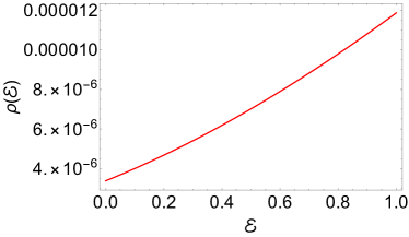
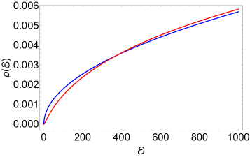
Figure 5: Vanishing density of states near $\mathcal{E}\approx 0$. Here, we consider $\mathcal{N}=1$ and $\Lambda=100$.

IV Summary and discussion

Applying the Wilsonian RG transformtion to an SYK model, we constructed an effective holographic dual field theory, which takes quantum corrections in the all-loop order. In particular, we justified our RG construction of this effective field theory, taking the UV limit and reproducing the perturbative result, given by the Schwarzian theory but in a self-consistent way. Taking the large $N$ limit in the holographic dual effective field theory, we obtain nonlinearly coupled bulk differential equations of motion for the three bi-local order-parameter fields, the self-energy function field $\Sigma(\tau-\tau^{\prime},z)$, the Green’s function field $G(\tau-\tau^{\prime},z)$, and the polarization function field $\Pi(\tau-\tau^{\prime},z)$, respectively. In addition, both UV and IR boundary conditions are derived self-consistently from the boundary effective action to complete the semiclassical analysis. Based on the conformal ansatz for the bi-local order-parameter fields at a given slice of the extradimension, we obtain essentially the same solution as that of the field theoretic large $N$ limit. However, their overall coefficients RG-flow along the extradimensional space, respectively, reflecting effects of higher-order quantum corrections. We suspect that the reason why the conformal ansatz works even in the introduction of higher order quantum corrections is the existence of the equivariant cohomology structure [50], but not clearly addressed in this study.

It turns out that the resulting IR fixed point shows an insulating behavior, where the fermion self-energy diverges to cause pseudogap physics for the dynamics of Majorana fermions. To understand physical implications, we investigated thermodynamics. We derived an effective onshell action from the holographic dual field theory, identified with a renormalized free energy functional in terms of the bi-local order-parameter fields. We argued that this renormalized free energy functional is a solution of both the Hamilton-Jacobi equation and the local RG equation, where the IR boundary condition is well applied and the Weyl anomaly is appropriately specified. Based on this effective free energy functional, we obtained the thermodynamic entropy and found the density of states. The vanishing density of states indicates that the RG flows of the collective dual order-parameter fields give rise to deviation from the Bekenstein-Hawking entropy behavior of the field theoretic large $N$ limit.

An immediate question is whether our holographic dual effective field theory can describe quantum chaos [61] or not. Recently, the quantum chaos in the dual holography has been more deeply understood by the study of the spectral form factor [62]. It turns out that the Euclidean wormhole geometry was proposed to be responsible for the quantum chaos in the spectral form factor perspective, more precisely, the $t-$linear increase (‘ramp’ behavior) in the spectral form factor [63]. Through the Euclidean wormhole, the spectra of both boundary conformal field theories are correlated, giving rise to so called the phenomena of level repulsion [64]. To catch the quantum chaotic behavior from our holographic dual field theory, we suspect that similar quantum gravity corrections have to be introduced in the study of the spectral form factor. We leave it as a fascinating future study along this direction of the research.

Appendix A Field theoretic analysis for an SYK model

A.1 Large $N$ analysis in the frequency domain

For completeness, we show the field theoretic anlysis for an SYK model, expected to clarify quantum corrections in the effective potential beyond the large $N$ analysis. We perform the Fourier transformtion in the partition function to obtain

$$\mathcal{Z}_{SYK}=\int D\Sigma(i\omega_{n})D\Pi(i\Omega_{n})DG(i\omega_{n})D\eta_{\alpha}(i\omega_{n})\exp\Big{[}-\Big{\{}\sum_{i\omega_{n}}\eta_{\alpha}(-i\omega_{n})\Big{(}-i\omega_{n}+q_{d}\Gamma_{J}\Sigma(i\omega_{n})\Big{)}\eta_{\alpha}(i\omega_{n})$$

$$-Nq_{d}\Gamma_{J}\sum_{i\omega_{n}}\Sigma(-i\omega_{n})G(i\omega_{n})+Nq_{d}\Gamma_{J}\sum_{i\omega_{n}}\frac{1}{\beta}\sum_{i\Omega_{n}}\Pi(i\Omega_{n})G(-i\omega_{n}-i\Omega_{n})G(i\omega_{n})+\frac{Nq_{d}\Gamma_{J}}{4}\sum_{i\Omega_{n}}\Pi(-i\Omega_{n})\Pi(i\Omega_{n})\Big{\}}\Big{]}.$$ (170)

Taking the Gaussian integration for the Majorana fermion field, we obtain

$$\mathcal{Z}_{SYK}=\int D\Sigma(i\omega_{n})D\Pi(i\Omega_{n})DG(i\omega_{n})\exp\Big{[}-N\Big{\{}-\frac{1}{2}\sum_{i\omega_{n}}\ln\Big{(}-i\omega_{n}+q_{d}\Gamma_{J}\Sigma(i\omega_{n})\Big{)}-q_{d}\Gamma_{J}\sum_{i\omega_{n}}\Sigma(-i\omega_{n})G(i\omega_{n})$$

$$+q_{d}\Gamma_{J}\sum_{i\omega_{n}}\frac{1}{\beta}\sum_{i\Omega_{n}}\Pi(i\Omega_{n})G(-i\omega_{n}-i\Omega_{n})G(i\omega_{n})+\frac{q_{d}\Gamma_{J}}{4}\sum_{i\Omega_{n}}\Pi(-i\Omega_{n})\Pi(i\Omega_{n})\Big{\}}\Big{]}.$$ (171)

In the large $N$ limit, we consider the saddle-point approximation and determine the fermion Green’s function, self-energy, and polarization function as follows

$$G(i\omega_{n})=\frac{1}{2}\frac{1}{i\omega_{n}-q_{d}\Gamma_{J}\Sigma(i\omega_{n})},$$ (172)

$$\Sigma(i\omega_{n})=2\frac{1}{\beta}\sum_{i\Omega_{n}}\Pi(i\Omega_{n})G(-i\omega_{n}-i\Omega_{n}),$$ (173)

$$\Pi(i\Omega_{n})=-2\frac{1}{\beta}\sum_{i\omega_{n}}G(i\omega_{n})G(-i\omega_{n}-i\Omega_{n}).$$ (174)

In the low frequency limit, one finds the conformal invariant solution, discussed in the main text.

A.2 Beyond the large $N$ analysis in the frequency domain

To take effects of quantum corrections beyond the large $N$ limit, we introduce perturbations for collective dual fields as follows

$$\Sigma(i\omega_{n})\longrightarrow\Sigma(i\omega_{n})+\delta\Sigma(i\omega_{n}),$$ (175)

$$\Pi(i\Omega_{n})\longrightarrow\Pi(i\Omega_{n})+\delta\Pi(i\Omega_{n}),$$ (176)

$$G(i\omega_{n})\longrightarrow G(i\omega_{n})+\delta G(i\omega_{n}).$$ (177)

Inserting these fluctuations into Eq. (170), we obtain

$$\mathcal{Z}_{SYK}[\Sigma(i\omega_{n}),\Pi(i\Omega_{n}),G(i\omega_{n})]=\int D\delta\Sigma(i\omega_{n})D\delta\Pi(i\Omega_{n})D\delta G(i\omega_{n})D\eta_{\alpha}(i\omega_{n})$$

$$\exp\Big{[}-\Big{\{}\sum_{i\omega_{n}}\eta_{\alpha}(-i\omega_{n})\Big{(}-i\omega_{n}+q_{d}\Gamma_{J}\Sigma(i\omega_{n})+q_{d}\Gamma_{J}\delta\Sigma(i\omega_{n})\Big{)}\eta_{\alpha}(i\omega_{n})-Nq_{d}\Gamma_{J}\sum_{i\omega_{n}}\Big{(}\Sigma(-i\omega_{n})+\delta\Sigma(-i\omega_{n})\Big{)}\Big{(}G(i\omega_{n})+\delta G(i\omega_{n})\Big{)}$$

$$+Nq_{d}\Gamma_{J}\sum_{i\omega_{n}}\frac{1}{\beta}\sum_{i\Omega_{n}}\Big{(}\Pi(i\Omega_{n})+\delta\Pi(i\Omega_{n})\Big{)}\Big{(}G(-i\omega_{n}-i\Omega_{n})+\delta G(-i\omega_{n}-i\Omega_{n})\Big{)}\Big{(}G(i\omega_{n})+\delta G(i\omega_{n})\Big{)}$$

$$+\frac{Nq_{d}\Gamma_{J}}{4}\sum_{i\Omega_{n}}\Big{(}\Pi(-i\Omega_{n})+\delta\Pi(-i\Omega_{n})\Big{)}\Big{(}\Pi(i\Omega_{n})+\delta\Pi(i\Omega_{n})\Big{)}\Big{\}}\Big{]}.$$ (178)

Performing the Gaussian integration for the Majorana fermion field and expanding the resulting logarithmic term for $\delta\Sigma(i\omega_{n})$ up to the second order, we obtain

$$\mathcal{Z}_{SYK}[\Sigma(i\omega_{n}),\Pi(i\Omega_{n}),G(i\omega_{n})]=\int D\delta\Sigma(i\omega_{n})D\delta\Pi(i\Omega_{n})D\delta G(i\omega_{n})\exp\Big{[}-N\Big{\{}-\frac{1}{2}\sum_{i\omega_{n}}\ln\Big{(}-2[\mathcal{G}(i\omega_{n})]^{-1}\Big{)}$$

$$+q_{d}\Gamma_{J}\sum_{i\omega_{n}}\mathcal{G}(i\omega_{n})\delta\Sigma(-i\omega_{n})+(q_{d}\Gamma_{J})^{2}\sum_{i\omega_{n}}\delta\Sigma(-i\omega_{n})\mathcal{G}(-i\omega_{n})\mathcal{G}(i\omega_{n})\delta\Sigma(i\omega_{n})-q_{d}\Gamma_{J}\sum_{i\omega_{n}}\Big{(}\Sigma(-i\omega_{n})+\delta\Sigma(-i\omega_{n})\Big{)}\Big{(}G(i\omega_{n})+\delta G(i\omega_{n})\Big{)}$$

$$+q_{d}\Gamma_{J}\sum_{i\omega_{n}}\frac{1}{\beta}\sum_{i\Omega_{n}}\Big{(}\Pi(i\Omega_{n})+\delta\Pi(i\Omega_{n})\Big{)}\Big{(}G(-i\omega_{n}-i\Omega_{n})+\delta G(-i\omega_{n}-i\Omega_{n})\Big{)}\Big{(}G(i\omega_{n})+\delta G(i\omega_{n})\Big{)}$$

$$+\frac{q_{d}\Gamma_{J}}{4}\sum_{i\Omega_{n}}\Big{(}\Pi(-i\Omega_{n})+\delta\Pi(-i\Omega_{n})\Big{)}\Big{(}\Pi(i\Omega_{n})+\delta\Pi(i\Omega_{n})\Big{)}\Big{\}}\Big{]},$$ (179)

where $\mathcal{G}(i\omega_{n})$ is the Majorana fermion Green’s function, given by

$$\mathcal{G}(i\omega_{n})=\frac{1}{2}\frac{1}{i\omega_{n}-q_{d}\Gamma_{J}\Sigma(i\omega_{n})}.$$ (180)

Here, we regard $\Sigma(i\omega_{n})$, $\Pi(i\Omega_{n})$, and $G(i\omega_{n})$ as background fields, identified with collective order parameter fields dual to composites of original fermion fields and determined self-consistently after the Gaussian integrations of $\int D\delta\Sigma(i\omega_{n})D\delta\Pi(i\Omega_{n})D\delta G(i\omega_{n})$.

A.3 Low energy effective action beyond the large $N$ limit in the frequency domain

Performing the Gaussian integral for $\int D\delta\Sigma(i\omega_{n})$, we obtain

$$\mathcal{Z}_{SYK}[\Sigma(i\omega_{n}),\Pi(i\Omega_{n}),G(i\omega_{n})]=\int D\delta\Pi(i\Omega_{n})D\delta G(i\omega_{n})\exp\Big{[}-N\Big{\{}-\frac{1}{2}\sum_{i\omega_{n}}\ln\Big{(}-2[\mathcal{G}(i\omega_{n})]^{-1}\Big{)}+\frac{1}{2N}\sum_{i\omega_{n}}\ln\Big{(}2(q_{d}\Gamma_{J})^{2}[\mathcal{G}(i\omega_{n})]^{2}\Big{)}$$

$$-\frac{1}{4}\sum_{i\omega_{n}}\Big{(}G(-i\omega_{n})-\mathcal{G}(-i\omega_{n})+\delta G(-i\omega_{n})\Big{)}[\mathcal{G}(i\omega_{n})]^{-2}\Big{(}G(i\omega_{n})-\mathcal{G}(i\omega_{n})+\delta G(i\omega_{n})\Big{)}-q_{d}\Gamma_{J}\sum_{i\omega_{n}}\Sigma(-i\omega_{n})\Big{(}G(i\omega_{n})+\delta G(i\omega_{n})\Big{)}$$

$$+q_{d}\Gamma_{J}\sum_{i\omega_{n}}\frac{1}{\beta}\sum_{i\Omega_{n}}\Big{(}\Pi(i\Omega_{n})+\delta\Pi(i\Omega_{n})\Big{)}\Big{(}G(-i\omega_{n}-i\Omega_{n})+\delta G(-i\omega_{n}-i\Omega_{n})\Big{)}\Big{(}G(i\omega_{n})+\delta G(i\omega_{n})\Big{)}$$

$$+\frac{q_{d}\Gamma_{J}}{4}\sum_{i\Omega_{n}}\Big{(}\Pi(-i\Omega_{n})+\delta\Pi(-i\Omega_{n})\Big{)}\Big{(}\Pi(i\Omega_{n})+\delta\Pi(i\Omega_{n})\Big{)}\Big{\}}\Big{]}.$$ (181)

Here, $\frac{1}{2N}\sum_{i\omega_{n}}\ln\Big{(}2(q_{d}\Gamma_{J})^{2}[\mathcal{G}(i\omega_{n})]^{2}\Big{)}$ corresponds to a $1/N$ correction, and $-\frac{1}{4}\sum_{i\omega_{n}}\Big{(}G(-i\omega_{n})-\mathcal{G}(-i\omega_{n})+\delta G(-i\omega_{n})\Big{)}[\mathcal{G}(i\omega_{n})]^{-2}\Big{(}G(i\omega_{n})-\mathcal{G}(i\omega_{n})+\delta G(i\omega_{n})\Big{)}$ gives a shift term due to the presence of the linear coupling term with $\delta\Sigma(i\omega_{n})$.

Performing the Gaussian integral for $\int D\delta G(i\omega_{n})$, we obtain

$$\mathcal{Z}_{SYK}[\Sigma(i\omega_{n}),\Pi(i\Omega_{n}),G(i\omega_{n})]=\int D\delta\Pi(i\Omega_{n})\exp\Big{[}-N\Big{\{}-\frac{1}{2}\sum_{i\omega_{n}}\ln\Big{(}-2[\mathcal{G}(i\omega_{n})]^{-1}\Big{)}$$

$$-q_{d}\Gamma_{J}\sum_{i\omega_{n}}\Sigma(-i\omega_{n})G(i\omega_{n})+q_{d}\Gamma_{J}\sum_{i\omega_{n}}\frac{1}{\beta}\sum_{i\Omega_{n}}\Pi(i\Omega_{n})G(-i\omega_{n}-i\Omega_{n})G(i\omega_{n})+\frac{q_{d}\Gamma_{J}}{4}\sum_{i\Omega_{n}}\Pi(-i\Omega_{n})\Pi(i\Omega_{n})$$

$$+\frac{1}{2N}\sum_{i\omega_{n}}\ln\Big{(}2(q_{d}\Gamma_{J})^{2}[\mathcal{G}(i\omega_{n})]^{2}\Big{)}-\frac{1}{4}\sum_{i\omega_{n}}\Big{(}G(-i\omega_{n})-\mathcal{G}(-i\omega_{n})\Big{)}[\mathcal{G}(i\omega_{n})]^{-2}\Big{(}G(i\omega_{n})-\mathcal{G}(i\omega_{n})\Big{)}$$

$$+\frac{1}{2N}\sum_{i\omega_{n}}\frac{1}{\beta}\sum_{i\omega^{\prime}_{n}}\ln\frac{1}{2}\Big{\{}[\mathcal{G}(i\omega_{n})]^{-2}\delta(\omega_{n}-\omega^{\prime}_{n})-4q_{d}\Gamma_{J}\Big{(}\Pi(i\omega_{n}-i\omega^{\prime}_{n})+\delta\Pi(i\omega_{n}-i\omega^{\prime}_{n})\Big{)}\Big{\}}$$

$$+\frac{1}{4}\sum_{i\omega_{n}}\frac{1}{\beta}\sum_{i\omega^{\prime}_{n}}\frac{1}{\beta}\sum_{i\nu_{n}}\frac{1}{\beta}\sum_{i\nu^{\prime}_{n}}\Big{\{}\delta(\omega_{n}-\nu_{n})\Big{(}[\mathcal{G}(i\omega_{n})]^{-2}\Big{(}G(i\omega_{n})-\mathcal{G}(i\omega_{n})\Big{)}+2q_{d}\Gamma_{J}\Sigma(i\omega_{n})\Big{)}-4q_{d}\Gamma_{J}\Big{(}\Pi(i\omega_{n}-i\nu_{n})+\delta\Pi(i\omega_{n}-i\nu_{n})\Big{)}\Big{\}}$$

$$\times\Big{\{}[\mathcal{G}(i\nu_{n})]^{-2}\delta(\nu_{n}-\nu^{\prime}_{n})-4q_{d}\Gamma_{J}\Big{(}\Pi(i\nu_{n}-i\nu^{\prime}_{n})+\delta\Pi(i\nu_{n}-i\nu^{\prime}_{n})\Big{)}\Big{\}}^{-1}$$

$$\Big{\{}\delta(\nu^{\prime}_{n}-\omega^{\prime}_{n})\Big{(}[\mathcal{G}(i\omega^{\prime}_{n})]^{-2}\Big{(}G(i\omega^{\prime}_{n})-\mathcal{G}(i\omega^{\prime}_{n})\Big{)}+2q_{d}\Gamma_{J}\Sigma(i\omega^{\prime}_{n})\Big{)}-4q_{d}\Gamma_{J}\Big{(}\Pi(i\nu^{\prime}_{n}-i\omega^{\prime}_{n})+\delta\Pi(i\nu^{\prime}_{n}-i\omega^{\prime}_{n})\Big{)}\Big{\}}$$

$$+\frac{q_{d}\Gamma_{J}}{4}\sum_{i\Omega_{n}}\delta\Pi(-i\Omega_{n})\delta\Pi(i\Omega_{n})+\frac{q_{d}\Gamma_{J}}{2}\sum_{i\Omega_{n}}\delta\Pi(i\Omega_{n})\Big{(}\Pi(-i\Omega_{n})+2\frac{1}{\beta}\sum_{i\omega_{n}}G(-i\omega_{n}-i\Omega_{n})G(i\omega_{n})\Big{)}\Big{\}}\Big{]},$$ (182)

where the newly generated $\ln-$term corresponds to a $1/N$ correction, and the corresponding shift term follows.

To consider the Gaussian integral for $\int D\delta\Pi(i\Omega_{n})$ in the above expression, we expand both the $\ln-$term and the shift term up to the second order in $\delta\Pi(i\Omega_{n})$. Then, we obtain

$$\mathcal{Z}_{SYK}[\Sigma(i\omega_{n}),\Pi(i\Omega_{n}),G(i\omega_{n})]$$

$$\approx\exp\Big{[}-N\Big{\{}-\frac{1}{2}\sum_{i\omega_{n}}\ln\Big{(}-2[\mathcal{G}(i\omega_{n})]^{-1}\Big{)}-q_{d}\Gamma_{J}\sum_{i\omega_{n}}\Sigma(-i\omega_{n})G(i\omega_{n})+q_{d}\Gamma_{J}\sum_{i\omega_{n}}\frac{1}{\beta}\sum_{i\Omega_{n}}\Pi(i\Omega_{n})G(-i\omega_{n}-i\Omega_{n})G(i\omega_{n})+\frac{q_{d}\Gamma_{J}}{4}\sum_{i\Omega_{n}}\Pi(-i\Omega_{n})\Pi(i\Omega_{n})\Big{\}}\Big{]}$$

$$\times\int D\delta\Pi(i\Omega_{n})\exp\Bigg{[}-N\Big{\{}\frac{1}{2N}\sum_{i\omega_{n}}\ln\Big{(}2(q_{d}\Gamma_{J})^{2}[\mathcal{G}(i\omega_{n})]^{2}\Big{)}+\frac{1}{2N}\sum_{i\omega_{n}}\frac{1}{\beta}\sum_{i\omega^{\prime}_{n}}\ln\frac{1}{2}\Big{\{}[\mathcal{G}(i\omega_{n})]^{-2}\delta(\omega_{n}-\omega^{\prime}_{n})-4q_{d}\Gamma_{J}\Pi(i\omega_{n}-i\omega^{\prime}_{n})\Big{\}}$$

$$-\frac{1}{4}\sum_{i\omega_{n}}\Big{(}G(-i\omega_{n})-\mathcal{G}(-i\omega_{n})\Big{)}[\mathcal{G}(i\omega_{n})]^{-2}\Big{(}G(i\omega_{n})-\mathcal{G}(i\omega_{n})\Big{)}$$

$$+\frac{1}{4}\sum_{i\omega_{n}}\frac{1}{\beta}\sum_{i\omega^{\prime}_{n}}\frac{1}{\beta}\sum_{i\nu_{n}}\frac{1}{\beta}\sum_{i\nu^{\prime}_{n}}\Big{\{}\delta(\omega_{n}-\nu_{n})\Big{(}[\mathcal{G}(i\omega_{n})]^{-2}\Big{(}G(i\omega_{n})-\mathcal{G}(i\omega_{n})\Big{)}+2q_{d}\Gamma_{J}\Sigma(i\omega_{n})\Big{)}-4q_{d}\Gamma_{J}\Pi(i\omega_{n}-i\nu_{n})\Big{\}}$$

$$\times\Big{\{}[\mathcal{G}(i\nu_{n})]^{-2}\delta(\nu_{n}-\nu^{\prime}_{n})-4q_{d}\Gamma_{J}\Pi(i\nu_{n}-i\nu^{\prime}_{n})\Big{\}}^{-1}\Big{\{}\delta(\nu^{\prime}_{n}-\omega^{\prime}_{n})\Big{(}[\mathcal{G}(i\omega^{\prime}_{n})]^{-2}\Big{(}G(i\omega^{\prime}_{n})-\mathcal{G}(i\omega^{\prime}_{n})\Big{)}+2q_{d}\Gamma_{J}\Sigma(i\omega^{\prime}_{n})\Big{)}-4q_{d}\Gamma_{J}\Pi(i\nu^{\prime}_{n}-i\omega^{\prime}_{n})\Big{\}}$$

$$+\frac{q_{d}\Gamma_{J}}{4}\sum_{i\omega_{n}}\frac{1}{\beta}\sum_{i\omega^{\prime}_{n}}\frac{1}{\beta}\sum_{i\nu_{n}}\frac{1}{\beta}\sum_{i\nu^{\prime}_{n}}\delta\Pi(i\omega_{n}-i\nu_{n})\Big{\{}\delta(\omega_{n}-\nu_{n})\delta(\omega^{\prime}_{n}-\nu^{\prime}_{n})+16q_{d}\Gamma_{J}\Big{(}[\mathcal{G}(i\nu_{n})]^{-2}\delta(\nu_{n}-\nu^{\prime}_{n})-4q_{d}\Gamma_{J}\Pi(i\nu_{n}-i\nu^{\prime}_{n})\Big{)}^{-1}\Big{\}}\delta\Pi(i\nu^{\prime}_{n}-i\omega^{\prime}_{n})$$

$$+\frac{q_{d}\Gamma_{J}}{2}\sum_{i\omega_{n}}\frac{1}{\beta}\sum_{i\omega^{\prime}_{n}}\frac{1}{\beta}\sum_{i\nu_{n}}\frac{1}{\beta}\sum_{i\nu^{\prime}_{n}}\delta\Pi(i\omega_{n}-i\nu_{n})\Bigg{(}\delta(\nu^{\prime}_{n}-\omega^{\prime}_{n})\Big{(}\Pi(i\nu_{n}-i\omega^{\prime}_{n})+2\frac{1}{\beta}\sum_{i\omega_{n}}G(-i\omega_{n}-i\nu_{n}+i\omega^{\prime}_{n})G(i\omega_{n})\Big{)}$$

$$-4\Big{\{}[\mathcal{G}(i\nu_{n})]^{-2}\delta(\nu_{n}-\nu^{\prime}_{n})-4q_{d}\Gamma_{J}\Pi(i\nu_{n}-i\nu^{\prime}_{n})\Big{\}}^{-1}\Big{\{}\delta(\nu^{\prime}_{n}-\omega^{\prime}_{n})\Big{(}[\mathcal{G}(i\omega^{\prime}_{n})]^{-2}\Big{(}G(i\omega^{\prime}_{n})-\mathcal{G}(i\omega^{\prime}_{n})\Big{)}+2q_{d}\Gamma_{J}\Sigma(i\omega^{\prime}_{n})\Big{)}-4q_{d}\Gamma_{J}\Pi(i\nu^{\prime}_{n}-i\omega^{\prime}_{n})\Big{\}}\Bigg{)}\Bigg{]}.$$ (183)

It is straightforward to take the Gaussian integral for $\int D\delta\Pi(i\Omega_{n})$, where the result is not shown here for the presentation perspective.

Appendix B Some regularizations and $\alpha$ $\&$ $a_{0}$

We consider the Fourier transformation of the fermionic conformal ansatz solution at finite temperature as

$$F_{\beta}(\Delta)=\int_{-\beta}^{\beta}d\tau\;\mbox{sgn}(\tau)e^{i\omega\tau}\left|\frac{\frac{\pi}{\beta}}{\sin\left(\frac{\pi\tau}{\beta}\right)}\right|^{\Delta}.$$ (184)

With $x=\frac{\pi\tau}{\beta}$, Eq. (184) becomes

$$F_{\beta}(\Delta) = \left(\frac{\pi}{\beta}\right)^{\Delta-1}\int_{-\pi}^{\pi}dx\;\frac{\mbox{sgn}(x)e^{ikx}}{\left|\sin\left(x\right)\right|^{\Delta}}=2i\left(\frac{\pi}{\beta}\right)^{\Delta-1}\int_{0}^{\pi}dx\;\frac{\sin(kx)}{\sin\left(x\right)^{\Delta}}.$$ (185)

Here, $k=\frac{\omega\beta}{\pi}$. For $x\to\pi$, we have $\frac{\sin(kx)}{\sin\left(x\right)^{\Delta}}\approx\frac{\sin(k\pi)}{(\pi-x)^{\Delta}}$. Then, we obtain $\int\frac{dx}{(\pi-x)^{\Delta}}=\frac{(\pi-x)^{1-\Delta}}{\Delta-1}$. We require $\Re(\Delta)<1$, otherwise, $\lim_{x\rightarrow\pi}\frac{(\pi-x)^{1-\Delta}}{\Delta-1}\rightarrow\infty$. We also have the following identity

$$\frac{1}{\sin(x)^{\Delta}}=\frac{1}{\Gamma(\Delta)}\int_{0}^{\infty}dt\;t^{\Delta-1}\exp(-t\sin(x))$$ (186)

with $\Re(\Delta)>0$. Otherwise, the above integral does not converge at $t=0$.

We substitute Eq. (186) into Eq. (185) and obtain

$$F_{\beta}(\Delta) = \frac{2i}{\Gamma(\Delta)}\left(\frac{\pi}{\beta}\right)^{\Delta-1}\int_{0}^{\pi}dx\;\sin(kx)\int_{0}^{\infty}dt\;t^{\Delta-1}\exp(-t\sin(x))$$ (187)

$$= \frac{2i}{\Gamma(\Delta)}\left(\frac{\pi}{\beta}\right)^{\Delta-1}\int_{0}^{\infty}dt\;t^{\Delta-1}\int_{0}^{\pi}dx\;\sin(kx)\exp(-t\sin(x))$$

$$= \frac{2i}{\Gamma(\Delta)}\left(\frac{\pi}{\beta}\right)^{\Delta-1}\int_{0}^{\infty}dt\;t^{\Delta-1}\int_{0}^{\pi}dx\;\sin(kx)\sum_{n=0}^{\infty}\frac{(-t)^{n}\sin(x)^{n}}{n!}$$

$$= \frac{2i}{\Gamma(\Delta)}\left(\frac{\pi}{\beta}\right)^{\Delta-1}\int_{0}^{\infty}dt\;t^{\Delta-1}\sum_{n=0}^{\infty}\frac{(-t)^{n}}{n!}\int_{0}^{\pi}dx\;\sin(kx)\sin(x)^{n},$$

where $0<\Re(\Delta)<1$.

If $n$ is even ($n=0,2,4,\cdots$), we obtain

$$\int_{0}^{\pi}dx\;\sin(kx)\sin(x)^{n}=\frac{(-1)^{\frac{n}{2}+1}n!(\cos(\pi k)-1)\Gamma\left(\frac{k}{2}-\frac{n}{2}\right)}{2^{n+1}\Gamma\left(\frac{k}{2}+\frac{n}{2}+1\right)}.$$ (188)

When $n$ is odd ($n=1,3,5,\cdots$), we have

$$\int_{0}^{\pi}dx\;\sin(kx)\sin(x)^{n}=\frac{(-1)^{\frac{n+1}{2}}n!\sin(\pi k)\Gamma\left(\frac{k}{2}-\frac{n}{2}\right)}{2^{n+1}\Gamma\left(\frac{k}{2}+\frac{n}{2}+1\right)}.$$ (189)

We substitute Eq. (188) and Eq. (189) into Eq. (187) and obtain

$$F_{\beta}(\Delta) = \frac{2i}{\Gamma(\Delta)}\left(\frac{\pi}{\beta}\right)^{\Delta-1}\int_{0}^{\infty}dt\;t^{\Delta-1}\sum_{n=0}^{\infty}\frac{(-1)^{n+1}t^{2n}\left(\frac{(\cos(\pi k)-1)\Gamma\left(\frac{k}{2}-n\right)}{\Gamma\left(\frac{k}{2}+n+1\right)}-\frac{t\sin(\pi k)\Gamma\left(\frac{k-1}{2}-n\right)}{2\Gamma\left(\frac{k+3}{2}+n\right)}\right)}{2^{2n+1}}$$ (190)

$$= \frac{i\pi}{\Gamma(\Delta)}\sin\left(\frac{\pi k}{2}\right)\left(\frac{\pi}{\beta}\right)^{\Delta-1}\int_{0}^{\infty}dt\;t^{\Delta-1}\left(\frac{2\,{}_{1}F_{2}{\left[\genfrac{.}{.}{0.0pt}{}{1}{1-\frac{k}{2}{\mathchar 44\relax}\mskip 4.0mu\frac{k}{2}+1};\frac{t^{2}}{4}\right]}}{\Gamma\left(1-\frac{k}{2}\right)\Gamma\left(\frac{k}{2}+1\right)}-\frac{t\,{}_{1}F_{2}{\left[\genfrac{.}{.}{0.0pt}{}{1}{\frac{3-k}{2}{\mathchar 44\relax}\mskip 4.0mu\frac{k+3}{2}};\frac{t^{2}}{4}\right]}}{\Gamma\left(\frac{3-k}{2}\right)\Gamma\left(\frac{k+3}{2}\right)}\right).$$

We recall the following identity [65]

$$\int\frac{z^{m}\,{}_{1}F_{2}{\left[\genfrac{.}{.}{0.0pt}{}{\mathit{a}}{\mathit{b}{\mathchar 44\relax}\mskip 4.0mu\mathit{c}};z\right]}}{\Gamma(\mathit{b})\Gamma(\mathit{c})}\,dz=\frac{z^{m+1}\Gamma(m+1)\,{}_{2}F_{3}{\left[\genfrac{.}{.}{0.0pt}{}{\mathit{a}{\mathchar 44\relax}\mskip 4.0mum+1}{\mathit{b}{\mathchar 44\relax}\mskip 4.0mu\mathit{c}{\mathchar 44\relax}\mskip 4.0mum+2};z\right]}}{\Gamma(\mathit{b})\Gamma(\mathit{c})\Gamma(m+2)}.$$ (191)

Utilizing this idenity, the indefinite integral in Eq. (191) reads

$$\int dt\;t^{\Delta-1}\left(\frac{2\;{}_{1}F_{2}{\left[\genfrac{.}{.}{0.0pt}{}{1}{1-\frac{k}{2}{\mathchar 44\relax}\mskip 4.0mu\frac{k}{2}+1};\frac{t^{2}}{4}\right]}}{\Gamma\left(1-\frac{k}{2}\right)\Gamma\left(\frac{k}{2}+1\right)}-\frac{t\;{}_{1}F_{2}{\left[\genfrac{.}{.}{0.0pt}{}{1}{\frac{3-k}{2}{\mathchar 44\relax}\mskip 4.0mu\frac{k+3}{2}};\frac{t^{2}}{4}\right]}}{\Gamma\left(\frac{3-k}{2}\right)\Gamma\left(\frac{k+3}{2}\right)}\right)$$ (192)

$$= \frac{1}{2}t^{\Delta}\left(\frac{2\Gamma\left(\frac{\Delta}{2}\right)\,{}_{2}F_{3}{\left[\genfrac{.}{.}{0.0pt}{}{1{\mathchar 44\relax}\mskip 4.0mu\frac{\Delta}{2}}{1-\frac{k}{2}{\mathchar 44\relax}\mskip 4.0mu\frac{k}{2}+1{\mathchar 44\relax}\mskip 4.0mu\frac{\Delta}{2}+1};\frac{t^{2}}{4}\right]}}{\Gamma\left(\frac{\Delta}{2}+1\right)\Gamma\left(1-\frac{k}{2}\right)\Gamma\left(\frac{k}{2}+1\right)}-\frac{t\;\Gamma\left(\frac{\Delta+1}{2}\right)\,{}_{2}F_{3}{\left[\genfrac{.}{.}{0.0pt}{}{1{\mathchar 44\relax}\mskip 4.0mu\frac{\Delta+1}{2}}{\frac{3-k}{2}{\mathchar 44\relax}\mskip 4.0mu\frac{k+3}{2}{\mathchar 44\relax}\mskip 4.0mu\frac{\Delta+3}{2}};\frac{t^{2}}{4}\right]}}{\Gamma\left(\frac{\Delta+3}{2}\right)\Gamma\left(\frac{3-k}{2}\right)\Gamma\left(\frac{k+3}{2}\right)}\right).$$

We recall the asymptotic formula for the ${}_{2}F_{3}$ hypergeometric function in the $|z|\rightarrow\infty$ limit as shown in Ref. [65]:

$${}_{2}F_{3}{\left[\genfrac{.}{.}{0.0pt}{}{a_{1}{\mathchar 44\relax}\mskip 4.0mua_{2}}{b_{1}{\mathchar 44\relax}\mskip 4.0mub_{2}{\mathchar 44\relax}\mskip 4.0mub_{3}};z\right]} = \frac{\Gamma(b_{1})\Gamma(b_{2})\Gamma(b_{3})}{2\sqrt{\pi}\Gamma(a_{1})\Gamma(a_{2})}(-z)^{\chi}\left(\exp(-i(\pi\chi+2\sqrt{-z}))+\exp(i(\pi\chi+2\sqrt{-z}))+\mathcal{O}\left(\frac{1}{\sqrt{-z}}\right)\right)$$ (193)

$$+\frac{\Gamma(b_{1})\Gamma(b_{2})\Gamma(b_{3})\Gamma(a_{2}-a_{1})}{\Gamma(b_{1}-a_{1})\Gamma(b_{2}-a_{1})\Gamma(b_{3}-a_{1})\Gamma(a_{2})}(-z)^{-a_{1}}\left(1+\mathcal{O}\left(\frac{1}{z}\right)\right)$$

$$+\frac{\Gamma(b_{1})\Gamma(b_{2})\Gamma(b_{3})\Gamma(a_{1}-a_{2})}{\Gamma(b_{1}-a_{2})\Gamma(b_{2}-a_{2})\Gamma(b_{3}-a_{2})\Gamma(a_{1})}(-z)^{-a_{2}}\left(1+\mathcal{O}\left(\frac{1}{z}\right)\right)$$

at $\chi=\frac{1}{2}\left(a_{1}+a_{2}-b_{1}-b_{2}-b_{3}+\frac{1}{2}\right)$ and wherein the case of simple poles (i.e., $a_{1}-a_{2}\not\in\mathbb{Z}$).

Substituting Eq. (193) into Eq. (192), we have

$$\int_{0}^{\infty}\;t^{\Delta-1}\left(\frac{2\;{}_{1}F_{2}{\left[\genfrac{.}{.}{0.0pt}{}{1}{1-\frac{k}{2}{\mathchar 44\relax}\mskip 4.0mu\frac{k}{2}+1};\frac{t^{2}}{4}\right]}}{\Gamma\left(1-\frac{k}{2}\right)\Gamma\left(\frac{k}{2}+1\right)}-\frac{t\;{}_{1}F_{2}{\left[\genfrac{.}{.}{0.0pt}{}{1}{\frac{3-k}{2}{\mathchar 44\relax}\mskip 4.0mu\frac{k+3}{2}};\frac{t^{2}}{4}\right]}}{\Gamma\left(\frac{3-k}{2}\right)\Gamma\left(\frac{k+3}{2}\right)}\right)$$ (194)

$$= \lim_{t\to\infty}2\left(\frac{\pi 2^{\Delta}\csc(\pi\Delta)}{\Gamma\left(\frac{1}{2}(k-\Delta+2)\right)\Gamma\left(-\frac{k}{2}-\frac{\Delta}{2}+1\right)}+t^{\Delta-2}\left(\frac{2k\sin\left(\frac{\pi k}{2}\right)}{\pi(\Delta-2)}-\frac{2t\cos\left(\frac{\pi k}{2}\right)}{\pi-\pi\Delta}+i\sqrt{\frac{2}{\pi}}e^{-t}\sqrt{t}\right)\right)$$

$$= \lim_{t\to\infty}2\left(\frac{\pi 2^{\Delta}\csc(\pi\Delta)}{\Gamma\left(\frac{1}{2}(k-\Delta+2)\right)\Gamma\left(-\frac{k}{2}-\frac{\Delta}{2}+1\right)}+\frac{2k\sin\left(\frac{\pi k}{2}\right)t^{\Delta-2}}{\pi(\Delta-2)}-\frac{2\cos\left(\frac{\pi k}{2}\right)t^{\Delta-1}}{\pi(1-\Delta)}\right).$$

When $0<\Re(\Delta)<1$, Eq. (194) becomes

$$\int_{0}^{\infty}\;t^{\Delta-1}\left(\frac{2\;{}_{1}F_{2}{\left[\genfrac{.}{.}{0.0pt}{}{1}{1-\frac{k}{2}{\mathchar 44\relax}\mskip 4.0mu\frac{k}{2}+1};\frac{t^{2}}{4}\right]}}{\Gamma\left(1-\frac{k}{2}\right)\Gamma\left(\frac{k}{2}+1\right)}-\frac{t\;{}_{1}F_{2}{\left[\genfrac{.}{.}{0.0pt}{}{1}{\frac{3-k}{2}{\mathchar 44\relax}\mskip 4.0mu\frac{k+3}{2}};\frac{t^{2}}{4}\right]}}{\Gamma\left(\frac{3-k}{2}\right)\Gamma\left(\frac{k+3}{2}\right)}\right)=\frac{\pi 2^{\Delta+1}\csc(\pi\Delta)}{\Gamma\left(\frac{1}{2}(k-\Delta+2)\right)\Gamma\left(-\frac{k}{2}-\frac{\Delta}{2}+1\right)}.$$ (195)

If $1<\Re(\Delta)<2$, Eq. (194) becomes

$$\int_{0}^{\infty}\;t^{\Delta-1}\left(\frac{2\;{}_{1}F_{2}{\left[\genfrac{.}{.}{0.0pt}{}{1}{1-\frac{k}{2}{\mathchar 44\relax}\mskip 4.0mu\frac{k}{2}+1};\frac{t^{2}}{4}\right]}}{\Gamma\left(1-\frac{k}{2}\right)\Gamma\left(\frac{k}{2}+1\right)}-\frac{t\;{}_{1}F_{2}{\left[\genfrac{.}{.}{0.0pt}{}{1}{\frac{3-k}{2}{\mathchar 44\relax}\mskip 4.0mu\frac{k+3}{2}};\frac{t^{2}}{4}\right]}}{\Gamma\left(\frac{3-k}{2}\right)\Gamma\left(\frac{k+3}{2}\right)}\right)$$ (196)

$$= \frac{\pi 2^{\Delta+1}\csc(\pi\Delta)}{\Gamma\left(\frac{1}{2}(k-\Delta+2)\right)\Gamma\left(-\frac{k}{2}-\frac{\Delta}{2}+1\right)}-\frac{4\cos\left(\frac{\pi k}{2}\right)}{\pi(1-\Delta)}\lim_{t\to\infty}t^{\Delta-1}.$$

We substitute Eq. (195) and Eq. (196) into Eq. (190) and obtain

$$F_{\beta}(\Delta) = \frac{i\pi}{\Gamma(\Delta)}\sin\left(\frac{\pi k}{2}\right)\left(\frac{\pi}{\beta}\right)^{\Delta-1}\frac{\pi 2^{\Delta+1}\csc(\pi\Delta)}{\Gamma\left(\frac{1}{2}(k-\Delta+2)\right)\Gamma\left(-\frac{k}{2}-\frac{\Delta}{2}+1\right)}$$ (197)

for $0<\Re(\Delta)<1$ and

$$F_{\beta}(\Delta) = \frac{i\pi}{\Gamma(\Delta)}\sin\left(\frac{\pi k}{2}\right)\left(\frac{\pi}{\beta}\right)^{\Delta-1}\left(\frac{\pi 2^{\Delta+1}\csc(\pi\Delta)}{\Gamma\left(\frac{1}{2}(k-\Delta+2)\right)\Gamma\left(-\frac{k}{2}-\frac{\Delta}{2}+1\right)}-\frac{4\cos\left(\frac{\pi k}{2}\right)}{\pi(1-\Delta)}\lim_{t\to\infty}t^{\Delta-1}\right)$$ (198)

for $1<\Re(\Delta)<2$. As a result, we obtain

$$F_{\beta}\left(1/2\right)=\frac{2i\sqrt{2}\pi\sin\left(\frac{\beta\omega}{2}\right)}{\sqrt{\frac{1}{\beta}}\Gamma\left(\frac{3}{4}-\frac{\beta\omega}{2\pi}\right)\Gamma\left(\frac{\beta\omega}{2\pi}+\frac{3}{4}\right)},$$ (199)

and

$$F_{\beta}\left(3/2\right)=-8i\sqrt{\frac{1}{\beta}}\left(\frac{\sqrt{2}\pi^{2}\sin\left(\frac{\beta\omega}{2}\right)}{\Gamma\left(\frac{\pi-2\beta\omega}{4\pi}\right)\Gamma\left(\frac{2\beta\omega+\pi}{4\pi}\right)}-\sin(\beta\omega)\lim_{t\to\infty}\sqrt{t}\right).$$ (200)

Putting $\omega=\frac{\pi(2n+1)}{\beta}$ into Eq. (199) and Eq. (200) and taking the following infinite summation, we have

$$\lim_{N\to\infty}\sum_{n=-N}^{N}F_{\beta}\left(1/2\right)F_{\beta}\left(3/2\right) =-\lim_{N\to\infty}\sum_{n=-N}^{N}\frac{16\cos 2(\pi n)\cos(2\pi n)\left(\pi^{2}+\lim_{t\to\infty}\sqrt{2}\sqrt{t}\sin(\pi n)\Gamma\left(-n-\frac{1}{4}\right)\Gamma\left(n+\frac{3}{4}\right)\right)}{\pi}$$ (201)

$$=-16\pi\lim_{N\to\infty}(2N+1).$$

The last expression will be regularized below.

We also consider the Fourier transformation of the bosonic conformal ansatz solution at finite temperature as

$$F_{\beta}(1)=\int_{-\beta}^{\beta}d\tau\;e^{i\omega\tau}\left|\frac{\frac{\pi}{\beta}}{\sin\left(\frac{\pi\tau}{\beta}\right)}\right|=\frac{2\pi}{\beta}\int_{0}^{\beta}\frac{\cos(\tau\omega)}{\sin\left(\frac{\pi\tau}{\beta}\right)}\,d\tau.$$ (202)

We should notice that $\frac{\cos(\tau\omega)}{\sin\left(\frac{\pi\tau}{\beta}\right)}$ does not converge at the end points of $\tau=0$ and $\tau=\beta$. To regularize this expression, we take an indefinite integral of it, and consider the limit of $\tau=0$ and $\tau=\beta$. Then, we renormalize the resulting expression.

The indefinite integral of Eq. (202) is given by

$$\frac{2\pi}{\beta}\int\frac{\cos(\tau\omega)}{\sin\left(\frac{\pi\tau}{\beta}\right)}\,d\tau=-2\pi e^{\frac{i\tau(\pi-\beta\omega)}{\beta}}\left(\frac{e^{2i\tau\omega}\,_{2}F_{1}\left(1,\frac{\beta\omega+\pi}{2\pi};\frac{1}{2}\left(\frac{\beta\omega}{\pi}+3\right);e^{\frac{2i\pi\tau}{\beta}}\right)}{\beta\omega+\pi}+\frac{\,{}_{2}F_{1}\left(1,\frac{\pi-\beta\omega}{2\pi};\frac{3}{2}-\frac{\beta\omega}{2\pi};e^{\frac{2i\pi\tau}{\beta}}\right)}{\pi-\beta\omega}\right).$$ (203)

As $\tau\rightarrow\beta$, Eq. (203) becomes

$$e^{-i\beta\omega}\left(-\left(\left(1+e^{2i\beta\omega}\right)\left(\lim_{\tau\to\beta}\log\left(1-\frac{\tau}{\beta}\right)+\gamma+\frac{i\pi}{2}+\log(2\pi)\right)\right)-e^{2i\beta\omega}\psi\left(\frac{\beta\omega+\pi}{2\pi}\right)-\psi\left(\frac{\pi-\beta\omega}{2\pi}\right)\right).$$ (204)

Here, $\psi(z)$ is the digamma function. As $\tau\rightarrow 0$, Eq. (203) becomes

$$2\left(\log\left(-\frac{2i\pi}{\beta}\right)+\lim_{\tau\to 0}\log(\tau)+\gamma\right)+\psi\left(\frac{\beta\omega+\pi}{2\pi}\right)+\psi\left(\frac{\pi-\beta\omega}{2\pi}\right).$$ (205)

We notice that $\lim_{\tau\to\beta}\log\left(1-\frac{\tau}{\beta}\right)$ and $\lim_{\tau\to 0}\log(\tau)$ do not converge. But, we can regularize them.

First, we consider

$$\log(x)=2\left(\xi+\frac{1}{3}\xi^{3}+\frac{1}{5}\xi^{5}+\cdots\right),$$ (206)

where $\xi=\frac{x-1}{x+1}$ at $\Re(x)>0$. Then, we have

$$\lim_{x\to\infty}\log(x) = 2\sum_{n=0}^{\infty}\frac{1}{2n+1}=2\lim_{\epsilon\to 0}\sum_{n=0}^{\infty}\frac{\exp(-\epsilon n)}{2n+1}=2\lim_{\epsilon\to 0}\exp(\epsilon/2)\operatorname{arctanh}(\exp(-\epsilon/2))$$ (207)

$$= 2\log(2)-\lim_{\epsilon\to 0}\log(\epsilon).$$

We consider

$$\log(x)=(x-1)-\frac{1}{2}(x-1)^{2}+\frac{1}{3}(x-1)^{3}-\frac{1}{4}(x-1)^{4}+\cdots$$ (208)

at $0<x<2$. Then, we have

$$\lim_{\epsilon\to 0}\log(\epsilon)=-(1+1/2+1/3+\cdots)=-\zeta(1).$$ (209)

Here, $\zeta(z)$ is the Riemann zeta function. A functional relation is given by

$$\zeta(s)=2^{s}\pi^{s-1}\sin\left(\frac{\pi s}{2}\right)\Gamma(1-s)\zeta(1-s)$$ (210)

at $0<\Re(s)<1$. Then, we have

$$\lim_{s\to 1}\zeta(s) = 2\zeta(0)\lim_{s\to 1}\Gamma(1-s)=-\lim_{s\to 1}\Gamma(1-s)=\gamma-\lim_{s\to 1}\frac{1}{1-s}$$ (211)

$$= \gamma+\lim_{s\to 1}\sum_{n=0}^{\infty}s^{n}=\gamma+\zeta(0)=\gamma-\frac{1}{2}.$$

So, Eq. (209) becomes

$$\lim_{\epsilon\to 0}\log(\epsilon)=-\gamma+\frac{1}{2}.$$ (212)

As a result, Eq. (207) becomes

$$\lim_{x\to\infty}\log(x)=2\log(2)+\gamma-\frac{1}{2}.$$ (213)

Substituting Eq. (212) into Eq. (204) and Eq. (205), we obtain

$$e^{-i\beta\omega}\left(-\left(\left(1+e^{2i\beta\omega}\right)\left(\lim_{\tau\to\beta}\log\left(1-\frac{\tau}{\beta}\right)+\gamma+\frac{i\pi}{2}+\log(2\pi)\right)\right)-e^{2i\beta\omega}\psi\left(\frac{\beta\omega+\pi}{2\pi}\right)-\psi\left(\frac{\pi-\beta\omega}{2\pi}\right)\right)$$ (214)

$$= e^{-i\beta\omega}\left(-\left(\left(\frac{1}{2}+\frac{i\pi}{2}+\log(2\pi)\right)\left(1+e^{2i\beta\omega}\right)\right)-e^{2i\beta\omega}\psi\left(\frac{\beta\omega+\pi}{2\pi}\right)-\psi\left(\frac{\pi-\beta\omega}{2\pi}\right)\right),$$

and

$$2\left(\log\left(-\frac{2i\pi}{\beta}\right)+\lim_{\tau\to 0}\log(\tau)+\gamma\right)+\psi\left(\frac{\beta\omega+\pi}{2\pi}\right)+\psi\left(\frac{\pi-\beta\omega}{2\pi}\right)$$ (215)

$$= \psi\left(\frac{\beta\omega+\pi}{2\pi}\right)+\psi\left(\frac{\pi-\beta\omega}{2\pi}\right)+2\log\left(-\frac{2i\pi}{\beta}\right)+1,$$

respectively.

Inserting Eq. (214) and Eq. (215) into Eq. (202, we obtain

$$F_{\beta}(1)=-(1+\log(4)+2\log(\pi))\cos(\beta\omega)-(\cos(\beta\omega)+1)\left(\psi\left(\frac{\beta\omega+\pi}{2\pi}\right)+\psi\left(\frac{\pi-\beta\omega}{2\pi}\right)\right)+2\log(\beta)-1-2\log(2\pi).$$ (216)

There is another way of regularization for Eq. (202).

$$F_{\beta}(1)=\frac{2\pi}{\beta}\int_{0}^{\beta}\frac{\cos(\tau\omega)}{\sin\left(\frac{\pi\tau}{\beta}\right)}\,d\tau=2\int_{0}^{\pi}\frac{\cos\left(\frac{\beta x\omega}{\pi}\right)}{\sin(x)}\,dx,$$ (217)

where $x=\frac{\pi\tau}{\beta}$ has been introduced. The indefinite integral of Eq. (217) is

$$-2\pi e^{\frac{ix(\pi-\beta\omega)}{\pi}}\left(\frac{e^{\frac{2i\beta x\omega}{\pi}}\,_{2}F_{1}\left(1,\frac{\beta\omega+\pi}{2\pi};\frac{\beta\omega}{2\pi}+\frac{3}{2};e^{2ix}\right)}{\beta\omega+\pi}+\frac{\,{}_{2}F_{1}\left(1,\frac{\pi-\beta\omega}{2\pi};\frac{3}{2}-\frac{\beta\omega}{2\pi};e^{2ix}\right)}{\pi-\beta\omega}\right).$$ (218)

Then, we obtain

$$\mbox{Eq. (\ref{qq:2})}=_{\tau\rightarrow\pi}\frac{1}{2}e^{-i\beta\omega}\left(-2e^{2i\beta\omega}\psi\left(\frac{\beta\omega+\pi}{2\pi}\right)-2\psi\left(\frac{\pi-\beta\omega}{2\pi}\right)-\left(1+e^{2i\beta\omega}\right)\left(2\lim_{\tau\to\pi}\log\left(1-\frac{x}{\pi}\right)+2\gamma+i\pi+\log\left(4\pi^{2}\right)\right)\right),$$ (219)

$$\mbox{Eq. (\ref{qq:2})}=_{\tau\rightarrow 0}\psi\left(\frac{\pi-\beta\omega}{2\pi}\right)+\psi\left(\frac{\beta\omega+\pi}{2\pi}\right)+2\lim_{\tau\to 0}\log(x)+2\gamma-i\pi+2\log(2).$$ (220)

Following the same regularization scheme above, we have

$$F_{\beta}(1)=-(\cos(\beta\omega)+1)(1+\log(4))-2\log(\pi)\cos(\beta\omega)-(\cos(\beta\omega)+1)\left(\psi\left(\frac{\beta\omega+\pi}{2\pi}\right)+\psi\left(\frac{\pi-\beta\omega}{2\pi}\right)\right).$$ (221)

Putting $\omega=\frac{2n\pi}{\beta}$ into Eq. (216) and taking the following infinite summation, we obtain

$$\lim_{N\to\infty}\sum_{n=-N}^{N}F_{\beta}^{2}\left(1\right)=\sum_{n=-N}^{N}\left(2\log\left(\frac{\beta}{2\pi}\right)-4\gamma+1-4\psi\left(n+\frac{1}{2}\right)\right)^{2}$$

$$=k^{2}(2N+1)-8k(N+1)\left(\psi\left(-N-\frac{1}{2}\right)-2\right)-8kN\psi\left(N+\frac{3}{2}\right)$$

$$+16\psi\left(\frac{1}{2}\right)^{2}+32\sum_{n=1}^{N}\psi\left(n+\frac{1}{2}\right)^{2}.$$ (222)

where $k=2\log\left(\frac{\beta}{2\pi}\right)-4\gamma+1$. In Eq. (222), we consider the following identity

$$\lim_{N\to\infty}\psi\left(-N-\frac{1}{2}\right)=\lim_{N\to\infty}\psi\left(N+\frac{3}{2}\right)=\log(N).$$ (223)

We also have

$$32\sum_{n=1}^{N}\psi\left(n+\frac{1}{2}\right)^{2}\approx 32\int_{1}^{N}\log^{2}\left(n+\frac{1}{2}\right)\,dn$$

$$=16\left(2\left(2+\log^{2}(2)+\log(4)\right)(N-1)+3\log(9)\left(1+\coth^{-1}(7)\right)\right)$$

$$+16(2N+1)\log(2N+1)\left(\log\left(\frac{1}{4}(2N+1)\right)-2\right).$$ (224)

Substituting Eq. (223) and Eq. (224) into Eq. (222), we obtain

$$\lim_{N\to\infty}\sum_{n=-N}^{N}F_{\beta}^{2}\left(1\right)$$

$$=k^{2}(2N+1)-8k(N+1)\left(\log(N)-2\right)-8kN\log(N)$$

$$+16\psi\left(\frac{1}{2}\right)^{2}+16\left(2\left(2+\log^{2}(2)+\log(4)\right)(N-1)+3\log(9)\left(1+\coth^{-1}(7)\right)\right)$$

$$+16(2N+1)\left(\log\left(N+\frac{1}{2}\right)+\log(2)\right)\left(\log\left(N+\frac{1}{2}\right)-2-\log(2)\right).$$ (225)

Eq. (213) results in

$$\lim_{N\to\infty}\log(N)=\lim_{N\to\infty}\log\left(N+\frac{1}{2}\right)=2\log(2)+\gamma-\frac{1}{2}.$$ (226)

In Eq. (225), we also consider the following regularization

$$\lim_{N\to\infty}N=\lim_{N\to\infty}\sum_{n=1}^{N}1=\zeta(0)=-\frac{1}{2}.$$ (227)

Substituting Eq. (226) and Eq. (227) into Eq. (225), we have

$$\lim_{N\to\infty}\sum_{n=-N}^{N}F_{\beta}^{2}\left(1\right)\approx 16\log(\beta)-43.1576.$$ (228)

Now, we consider the other regularization. Putting $\omega=\frac{2n\pi}{\beta}$ into Eq. (221) and taking the following infinite summation, we have

$$\lim_{N\to\infty}\sum_{n=-N}^{N}F_{\beta}^{2}\left(1\right)=\sum_{n=-N}^{N}\left(4\psi\left(n+\frac{1}{2}\right)+2(1+\log(4\pi))\right)^{2}$$

$$=t^{2}(2N+1)+8t\left(-2(N+1)+(N+1)\psi\left(-N-\frac{1}{2}\right)+N\psi\left(N+\frac{3}{2}\right)\right)$$

$$+16\psi\left(\frac{1}{2}\right)^{2}+32\sum_{n=1}^{N}\psi\left(n+\frac{1}{2}\right)^{2}.$$ (229)

Substituting Eq. (223) and Eq. (224) into Eq. (229), we obtain

$$\lim_{N\to\infty}\sum_{n=-N}^{N}F_{\beta}^{2}\left(1\right)$$

$$=t^{2}(2N+1)+8t(-2(N+1)+(N+1)\log(N)+N\log(N))+16\psi\left(\frac{1}{2}\right)^{2}$$

$$+16\left(2\left(2+\log^{2}(2)+\log(4)\right)(N-1)+3\log(9)\left(1+\coth^{-1}(7)\right)\right)$$

$$+16(2N+1)\left(\log\left(N+\frac{1}{2}\right)-2-\log(2)\right)\left(\log\left(N+\frac{1}{2}\right)+\log(2)\right).$$ (230)

Taking Eq. (226) and Eq. (227) into Eq. (230), we have

$$\lim_{N\to\infty}\sum_{n=-N}^{N}F_{\beta}^{2}\left(1\right)\approx-59.777.$$ (231)

Finally, we introduce

$$\alpha=-2q_{d}\Gamma_{J}\frac{\lim_{N\to\infty}\sum_{n=-N}^{N}F_{\beta}\left(1/2\right)F_{\beta}\left(3/2\right)}{\lim_{N\to\infty}\sum_{n=-N}^{N}1},$$ (232)

and

$$a_{0}=\frac{\lim_{N\to\infty}\sum_{n=-N}^{N}F_{\beta}\left(1/2\right)F_{\beta}\left(3/2\right)}{\lim_{N\to\infty}\sum_{n=-N}^{N}F_{\beta}^{2}\left(1\right)}.$$ (233)

Inserting Eq. (201) into Eq. (232), we obtain

$$\alpha=32\pi q_{d}\Gamma_{J}.$$ (234)

Let’s take Eq. (201), Eq. (227), and Eq. (228) into Eq. (233) with $N\rightarrow\infty$. Then, we obtain

$$a_{0}=-\frac{16\pi}{4\log^{2}(\beta)-27.355\log(\beta)+62.767}.$$ (235)

For the other regularization, we have

$$a_{0}=-0.52636.$$ (236)

References

• [1] J. D. Bekenstein, Black holes and the second law, Lett. Nuovo Cim. 4, 737 (1972).
• [2] J. D. Bekenstein, Black holes and entropy, Phys. Rev. D 7, 2333 (1973).
• [3] J. D. Bekenstein, Generalized second law of thermodynamics in black hole physics, Phys. Rev. D 9, 3292 (1974).
• [4] J. M. Bardeen, B. Carter, and S. W. Hawking, The four laws of black hole mechanics, Commun. Math. Phys 31, 161 (1973).
• [5] S. W. Hawking, Black holes and thermodynamics, Phys. Rev. D 13, 191 (1976).
• [6] S. W. Hawking, Particle creation by black holes, Commun. Math. Phys 43, 199 (1975).
• [7] S. W. Hawking, Breakdown of predictability in gravitational collapse, Phys. Rev. D 14, 2460 (1976).
• [8] J. M. Maldacena, The Large $N$ Limit of Superconformal Field Theories and Supergravity, Int. J. Theor. Phys. 38, 1113 (1999).
• [9] S. S. Gubser, I. R. Klebanov, and A. M. Polyakov, textitGauge Theory Correlators from Non-Critical String Theory, Phys. Lett. B 428, 105 (1998).
• [10] E. Witten, Anti De Sitter Space And Holography, Adv. Theor. Math. Phys. 2, 253 (1998).
• [11] O. Aharony, S. S. Gubser, J. Maldacena, H. Ooguri, and Y. Oz, Large $N$ Field Theories, String Theory and Gravity, Phys. Rep. 323, 183 (2000).
• [12] M. Bianchi, D. Z. Freedman, and K. Skenderis, Holographic renormalization, Nucl. Phys. B 631, 159 (2002).
• [13] J. de Boer, E. P. Verlinde, and H. L. Verlinde, On the Holographic Renormalization Group, JHEP 08, 003 (2000).
• [14] E. P. Verlinde and H. L. Verlinde, RG flow, gravity and the cosmological constant, JHEP 05, 034 (2000).
• [15] Alberto Zaffaroni, AdS black holes, holography and localization, Living Rev. Relativ. 23, 2 (2020); arXiv:1902.07176v3 [hep-th].
• [16] Justin R. David, Gautam Mandal, and Spenta R. Wadia, Microscopic formulation of black holes in string theory, Physics Reports 369, 549 (2002).
• [17] A. Strominger and C. Vafa, Microscopic origin of the Bekenstein-Hawking entropy, Phys. Lett. B 379, 99 (1996).
• [18] F. Benini, K. Hristov, and A. Zaffaroni, Black hole microstates in AdS4 from supersymmetric localization, JHEP 05, 054 (2016).
• [19] A. Cabo-Bizet, D. Cassani, D. Martelli, and S. Murthy, Microscopic origin of the Bekenstein-Hawking entropy of supersymmetric AdS5 black holes, JHEP 10, 062 (2019).
• [20] S. Choi, J. Kim, S. Kim, and J. Nahmgoong, Large AdS black holes from QFT, arXiv:1810.12067 [hep-th].
• [21] F. Benini and P. Milan, Black holes in 4d N = 4 Super-Yang-Mills, Phys. Rev. X 10, 021037 (2020).
• [22] S. M. Hosseini, K. Hristov, and A. Zaffaroni, An extremization principle for the entropy of rotating BPS black holes in AdS5, JHEP 07, 106 (2017).
• [23] S. Choi, C. Hwang, S. Kim, and J. Nahmgoong, Entropy functions of BPS black holes in AdS4 and AdS6, J. Korean Phys. Soc. 76, 101 (2020); https://doi.org/10.3938/jkps.76.101; arXiv:1811.02158.
• [24] Matthias Blau, Lecture Notes on General Relativity, http://www.blau.itp.unibe.ch/GRLecturenotes.html (“unpublished”).
• [25] Matthew Heydeman, Luca V. Iliesiu, Gustavo J. Turiaci, and Wenli Zhao, The statistical mechanics of near-BPS black holes, J. Phys. A 55, 014004 (2022).
• [26] Jan Boruch, Matthew T. Heydeman, Luca V. Iliesiu, and Gustavo J. Turiaci, BPS and near-BPS black holes in AdS5 and their spectrum in $\mathcal{N}=4$ SYM, arXiv:2203.01331v1 [hep-th].
• [27] Antoine Georges, Gabriel Kotliar, Werner Krauth, and Marcelo J. Rozenberg, Dynamical mean-field theory of strongly correlated fermion systems and the limit of infinite dimensions, Rev. Mod. Phys. 68, 13 (1996).
• [28] Ki-Seok Kim, Mitsuhiro Nishida, and Yoonseok Choun, Renormalization group flow to effective quantum mechanics at IR in an emergent dual holographic description for spontaneous chiral symmetry breaking, arXiv:2210.10277v2 [hep-th].
• [29] Ki-Seok Kim and Shinsei Ryu, Nonequilibrium thermodynamics perspectives for the monotonicity of the renormalization group flow, Phys. Rev. D 108, 126022 (2023).
• [30] Ki-Seok Kim, Beyond quantum chaos in emergent dual holography, Phys. Rev. D 106, 126014 (2022).
• [31] Ki-Seok Kim, Shinsei Ryu, and Kanghoon Lee, Emergent dual holographic description as a nonperturbative generalization of the Wilsonian renormalization group, Phys. Rev. D 105, 086019 (2022).
• [32] Ki-Seok Kim and Shinsei Ryu, Entanglement transfer from quantum matter to classical geometry in an emergent holographic dual description of a scalar field theory, JHEP05(2021)260, https://doi.org/10.1007/JHEP05(2021)260.
• [33] Ki-Seok Kim, Emergent dual holographic description for interacting Dirac fermions in the large $N$ limit, Phys. Rev. D 102, 086014 (2020).
• [34] Ki-Seok Kim, Geometric encoding of renormalization group $\beta$-functions in an emergent holographic dual description, Phys. Rev. D 102, 026022 (2020).
• [35] Ki-Seok Kim, Emergent geometry in recursive renormalization group transformations, Nucl. Phys. B 959, 115144 (2020).
• [36] Ki-Seok Kim, Suk Bum Chung, Chanyong Park, and Jae-Ho Han, A non-perturbative field theory approach for the Kondo effect: Emergence of an extra dimension and its implication for the holographic duality conjecture, Phys. Rev. D 99, 105012 (2019).
• [37] K.-S. Kim, M. Park, J. Cho, and C. Park, An emergent geometric description for a topological phase transition in the Kitaev superconductor model, Phys. Rev. D 96, 086015 (2017).
• [38] K.-S. Kim and C. Park, Emergent geometry from field theory: Wilson’s renormalization group revisited, Phys. Rev. D 93, 121702 (2016).
• [39] Subir Sachdev and Jinwu Ye, Gapless spin-fluid ground state in a random quantum Heisenberg magnet, Phys. Rev. Lett. 70, 3339 (1993).
• [40] A. Kitaev, Talks Given at the Fundamental Physics Prize Symposium and KITP Seminars, https://www.youtube.com/watch?v=OQ9qN8j7EZI, http://online.kitp.ucsb.edu/online/joint98/kitaev/, http://online.kitp.ucsb.edu/online/entangled15/kitaev.
• [41] Debanjan Chowdhury, Antoine Georges, Olivier Parcollet, and Subir Sachdev, Sachdev-Ye-Kitaev models and beyond: Window into non-Fermi liquids, Rev. Mod. Phys. 94, 035004 (2022).
• [42] Vladimir Rosenhaus, An introduction to the SYK model, J. Phys. A: Math. Theor. 52, 323001 (2019).
• [43] Olivier Parcollet and Antoine Georges, Non-Fermi-liquid regime of a doped Mott insulator, Phys. Rev. B 59, 5341 (1999).
• [44] T. F. Rosenbaum, R. F. Milligan, M. A. Paalanen, G. A. Thomas, R. N. Bhatt, and W. Lin, Metal-insulator transition in a doped semiconductor, Phys. Rev. B 27, 7509 (1983).
• [45] H. von Loehneysen, Current issues in the physics of heavily doped semiconductors at the metal–insulator transition, Phil. Trans. R. Soc. A. 356, 139 (1998).
• [46] J. Maldacena and D. Stanford, Remarks on the Sachdev-Ye-Kitaev model, Phys. Rev. D 94, 106002 (2016).
• [47] K. Jensen, Chaos in AdS2 Holography, Phys. Rev. Lett. 117, 111601 (2016).
• [48] J. Maldacena, D. Stanford, and Z. Yang, Conformal Symmetry and its Breaking in Two Dimensional Nearly Anti-de-Sitter Space, arXiv:1606.01857 [hep-th].
• [49] J. Engelsoy, T. G. Mertens, and H. Verlinde, An Investigation of AdS2 Backreaction and Holography, JHEP 07, 139 (2016).
• [50] Douglas Stanford and Edward Witten, Fermionic localization of the schwarzian theory, JHEP 10, 008 (2017).
• [51] Euihun Joung, Prithvi Narayan, and Junggi Yoon, Gravitational Edge Mode in Asymptotically AdS2: JT Gravity Revisited, arXiv:2304.06088v2 [hep-th].
• [52] R. Jackiw, Lower Dimensional Gravity, Nucl. Phys. B 252, 343 (1985).
• [53] C. Teitelboim, Gravitation and Hamiltonian Structure in Two Space-Time Dimensions, Phys. Lett. B 126, 41 (1983).
• [54] A. Almheiri and J. Polchinski, Models of AdS2 Backreaction and Holography, JHEP 11, 014 (2015).
• [55] D. Grumiller, W. Kummer, D. V. Vassilevich, Dilaton Gravity in Two Dimensions, Phys. Rept. 369, 327 (2002).
• [56] Alexei Kitaev and S. Josephine Suh, The soft mode in the Sachdev-Ye-Kitaev model and its gravity dual, JHEP 05, 183 (2018).
• [57] I. Papadimitriou, Lectures on Holographic Renormalization, Springer Proc. Phys. 176 (2016) 131-181, DOI: 10.1007/978-3-319-31352-8$\_$4.
• [58] H. Osborn, Weyl consistency conditions and a local renormalisation group equation for general renormalisable field theories, Nucl. Phys. B 363, 486 (1991).
• [59] G. Shore, The c and a-Theorems and the Local Renormalisation Group, (SpringerBriefs in Physics, 2017), ISBN 978-3-319-54000-9, DOI: 10.1007/978-3-319-54000-9 [arXiv:1601.06662v2 [hep-th]].
• [60] https://en.wikipedia.org/wiki/Barnes$\_$G-function.
• [61] Luca D’Alessio, Yariv Kafri, Anatoli Polkovnikov, and Marcos Rigol, From Quantum Chaos and Eigenstate Thermalization to Statistical Mechanics and Thermodynamics, Adv. Phys. 65, 239 (2016).
• [62] Jordan S. Cotler, Guy Gur-Ari, Masanori Hanada, Joseph Polchinski, Phil Saad, Stephen H. Shenker, Douglas Stanford, Alexandre Streicher, and Masaki Tezuka, Black holes and random matrices, JHEP 05, 188 (2017).
• [63] P. Saad, S. H. Shenker, and D. Stanford, A semiclassical ramp in SYK and in gravity, arXiv:1806.06840; P. Saad, S. H. Shenker, and D. Stanford, JT gravity as a matrix integral, arXiv:1903.11115.
• [64] Alexander Altland and Julian Sonner, Late time physics of holographic quantum chaos, SciPost Phys. 11, 034 (2021); Julian Sonner’s lecture series in Holography 2021: Quantum Matter, Information, and Spacetime, $https://www.apctp.org/theme/d/html/activities/activities01\_read.php?id=1518\&page=1$.
• [65] Ian Thompson, Frank W. J. Olver, Daniel W. Lozier, Ronald F. Boisvert, and Charles W. Clark, NIST Handbook of Mathematical Functions, (Taylor & Francis, 2011).