Uniqueness, stability and algorithm for an inverse wave-number-dependent source problems

Abstract

This paper is concerned with an inverse wave-number-dependent/frequency-dependent source problem for the Helmholtz equation. In $d$-dimensions ($d=2,3$), the unknown source term is supposed to be compactly supported in spatial variables but independent on $x_{d}$. The dependance of the source function on $k$ is supposed to be unknown. Based on the Dirichlet-Laplacian method and the Fourier-Transform method, we develop two efficient non-iterative numerical algorithms to recover the wave-number-dependent source. Uniqueness and increasing stability analysis are proved. Numerical experiments are conducted to illustrate the effectiveness and efficiency of the proposed method.

Keywords: inverse source problem, wave-number-dependent source, Helmholtz equation, increasing stability.

1 Introduction and motivations

1.1 Statement of the problem

Consider a time-dependent acoustic wave radiating problem in ${\mathbb{R}}^{d}$ ($d=2,3$) with the homogeneous initial conditions

$$\left\{\begin{aligned} \partial^{2}_{t}U(x,t)-\Delta U(x,t)=-S(x,t),\quad x&\in{\mathbb{R}}^{d},\,t>0,\\ U(x,0)=\partial_{t}U(x,0)=0,\quad x&\in{\mathbb{R}}^{d},\end{aligned}\right.$$ (1.1)

where $x=(\widetilde{x},x_{d})$, $\widetilde{x}=(x_{1},x_{2},\cdots,x_{d-1})\in{\mathbb{R}}^{d-1}$ and $U(x,t)$ represents the wave field. To state the motivation of our problem, we suppose that the source term $S(x,t)$ is excited by a moving point source along the trajectory $a(t):{\mathbb{R}}_{+}\longmapsto{\mathbb{R}}^{d}$ for $t\in[0,T]$. More precisely, we suppose that the source function takes the form (see e.g., [21])

$$S(x,t)=\delta(x-a(t))\chi(t),$$ (1.2)

where the symbol $\delta$ is the Dirac delta function and $\chi(t)$ the characteristic function given by

$$\chi(t)=\left\{\begin{array}[]{lll}1,\qquad t\in{[0,T]},\\ 0,\qquad t\notin{[0,T]}.\end{array}\right.$$

Assume further that the point source moves on the hyperplane $x_{d}=h$ for some $h>0$ so that the trajectory function can be written as $a(t)=(\widetilde{a}(t),h)$, where $\widetilde{a}(t):{\mathbb{R}}^{+}\longmapsto{\mathbb{R}}^{d-1}$ is supposed to be a smooth function. Then the source term can be physically approximated by

$$S(x,t)=\delta(\widetilde{x}-\widetilde{a}(t))\,\chi(t)\,\delta(x_{d}-h)\sim F(\tilde{x},t)g(x_{d})$$

where the Delta function is approximated by functions with a compact support in the distributional sense. Below we shall identity $S(x,t)$ with $F(\tilde{x},t)g(x_{d})$ for the convenience of mathematical analysis. The solution of problem (1.1) can be given explicitly as

$$U(x,t)=-\int_{{\mathbb{R}}^{+}}\int_{{\mathbb{R}}^{d-1}}G_{d}(x-y;t-\tau)S(x,\tau)dyd\tau,\quad x\in{\mathbb{R}}^{d},\,t>0,$$

where

$$G_{d}(x;t)=\left\{\begin{aligned} &\dfrac{H(t-|x|)}{2\pi\sqrt{t^{2}-|x|^{2}}},&\qquad d=2;\\ &\dfrac{\delta(t-|x|)}{4\pi|x|},&\qquad d=3,\end{aligned}\qquad x\in{\mathbb{R}}^{d},\,x\neq 0,\right.$$

is the fundamental solution to the wave equation in ${\mathbb{R}}^{d}$ and $H(\tau)$ is the Heaviside function

$$H(\tau)=\left\{\begin{array}[]{l}1,\qquad\tau\geq 0,\\ 0,\qquad\tau<0.\par\end{array}\right.$$

The $n$-dimensional($n=1,2$) Fourier and inverse Fourier transform in this paper are defined by

$$(\mathcal{F}_{t}\,\rho)(k) = \dfrac{1}{(2\pi)^{d/2}}\int_{{\mathbb{R}}^{n}}\rho(t)e^{-ikt}\,dt,\quad k\in{\mathbb{R}}^{d},$$

$$(\mathcal{F}_{k}^{-1}q)(t) = \dfrac{1}{(2\pi)^{d/2}}\int_{{\mathbb{R}}^{n}}q(k)e^{ikt}\,dk,\quad\,\,\,t\in{\mathbb{R}}^{d},$$

where the subscript denotes the variable to be Fourier or inverse Fourier transformed. The inverse Fourier transform of $S(x,t)$ is given by

$$(\mathcal{F}_{t}^{-1}S)(x,k)\sim(\mathcal{F}_{t}^{-1}F)(\widetilde{x},k)g(x_{d}):=f(\widetilde{x},k)g(x_{d}).$$

It is obvious that the spatial function $\widetilde{x}\longmapsto f(\widetilde{x},k)$ is compactly supported for all $k>0$. The temporal inverse Fourier transform of $U(x,t)$ is given by

$$u(x,k):=(\mathcal{F}^{-1}_{t}U)(x,k)=-\dfrac{1}{\sqrt{2\pi}}\int_{{\mathbb{R}}^{d}}\Phi_{d}(x-y;k)f(\widetilde{y},k)g(y_{d})dy,\qquad x\in{\mathbb{R}}^{d},\,k>0,$$ (1.5)

where $\Phi_{d}(x;k)$ is the fundamental solution to the Helmholtz equation $(\Delta+k^{2})u=0$ in ${\mathbb{R}}^{d}$, given by

$$\Phi_{d}(x-y;k)=(\mathcal{F}^{-1}_{t}G_{d})=\left\{\begin{aligned} &\dfrac{i}{4}H^{(1)}_{0}(k|x-y|),&\quad d=2;\\ &\dfrac{e^{ik|x-y|}}{4\pi|x-y|},&\quad d=3,\end{aligned}\qquad x,y\in{\mathbb{R}}^{d},\,x\neq y.\right.$$

Here $H_{0}^{(1)}$ is the first kind Hankel function of order zero. Applying the inverse Fourier transform w.r.t. the time variable to the wave equation (1.1), we conclude that

$$\Delta u(x,k)+k^{2}u(x,k)=f(\widetilde{x},k)g(x_{d}),\qquad x\in{\mathbb{R}}^{d},\,k>0.$$ (1.6)

Moreover, the radiated field $u(x,k)$ satisfies the following Sommerfeld radiation condition

$$\lim\limits_{r\rightarrow\infty}r^{\frac{d-1}{2}}(\partial_{r}u-iku)=0,\quad r=|x|,$$ (1.7)

which holds uniformly in all directions $\hat{x}=x/{|x|}\in{\mathbb{S}}^{d-1}:=\{x\in{\mathbb{R}}^{d}:|x|=1\}$.

Denote by $\Omega:=B_{R}\subset{\mathbb{R}}^{d}$ the sphere centered at the origin with the radius $R>0$ and by $\partial B_{R}:=\{x\in{\mathbb{R}}^{d}:\ |x|=R\}$ the boundary of $B_{R}$. The unit normal vector $\nu$ at the boundary $\partial B_{R}$ is supposed to direct into the exterior of $B_{R}$. Define two non-empty subsets $\widetilde{D}\subset{\mathbb{R}}^{d-1}$ and $H\subset{\mathbb{R}}_{+}$ such that $\widetilde{D}\times H\subset\subset B_{R}$. We make the following assumptions on the source functions $f(\widetilde{x},k)$ and $g(x_{d})$:

Assumption 1.1.

It holds that

• $f(\widetilde{x},k)g(x_{d})\in L^{2}(B_{R})$ and the function $g$ does not vanish identically; $g$ is a priori known;

• ${\rm supp}\,\,g=\overline{H}$, ${\rm supp}\,\,f(\cdot,k)=\overline{\widetilde{D}}$ for all $k>0$ and $f(\widetilde{x},k)$ is analytic with respect to $k$.

It is obvious that $f(\cdot,k)\in L^{2}(\widetilde{B}_{R})$ and $g\in L^{2}([-R,R])$ where $\widetilde{B}_{R}:=\{\widetilde{x}\in{\mathbb{R}}^{d-1}:\ x=(\widetilde{x},x_{d})\in B_{R},\ x_{d}=0\}$. In this paper, we are interested in the following inverse problem:

(IP): Determine the source function $f(\widetilde{x},k)\in L^{2}(\widetilde{B}_{R})$ from knowledge of the multi-frequency near-field measurement

$$\big{\{}u(x,k):\ x\in\partial B_{R},\ k\in[k_{\min},k_{\max}],\ m=1,2,\cdots,M\big{\}},$$ (1.8)

where $[k_{\min},k_{\max}]$ denotes an interval of available wavenumbers with $0<k_{\min}<k_{\max}$.

1.2 Literature review

Inverse source problems in wave propagation are of great importance in various scientific and engineering fields such as antenna design and synthesis, medical imaging and photo-acoustic tomography [20, 4, 17, 30]. Consequently, a great deal of mathematical and numerical results are available, especially for wave-number-independent source problems of the Helmholtz equation. In general, it is known that there is an obstruction to uniqueness for inverse source problems with single-frequency data due to the existence of non-radiating sources [25, 11]. Computationally, a more serious issue is the stability analysis, i.e., to quantify how does a small variation of the data lead to a huge error in the reconstruction. Hence it is crucial to study the stability of inverse source problems. Recently, it has been realized that the use of multi-frequency data is an effective approach to overcome the difficulties of non-uniqueness and instability which are encountered at a single frequency. In [6], Bao et al. initialized the mathematical study on the stability of the inverse wave-number-independent source problem for the Helmholtz equation by using multi-frequency data. In the recent works [6, 12, 14, 5, 22], uniqueness and stability results have been proved for the recovery of the source term from the multi-frequency boundary measurements. In [6], the authors treated an interior inverse source problem for the Helmholtz equation from boundary Cauchy data for multiple wave numbers and showed an increasing stability result for the problem under consideration. A uniqueness result and numerical algorithm for recovering the location and shape of a supported acoustic source function from boundary measurements at many frequencies were shown in [12]. The approach of [14] also provides inspirations for establishing uniqueness result. It was shown that an acoustic source of the form $S(x,k)=f(x)g(k)$ can be identified uniquely by measurements of the acoustic field on boundary. The proof relies on complete sets of solutions to the homogeneous Helmholtz equation. An error estimate and a numerical algorithm for the solution are presented. Several numerical methods for solving the multi-frequency inverse source problem have been proposed. We refer the reader to [31, 7] for the Fourier method and recursive algorithm. In addition, there are other uniqueness, increasing stability and algorithm results, see also [15, 23, 27, 28, 26, 24, 10, 13, 16, 1, 2, 8] and the references therein.

To the best of our knowledge, there are only few works on inverse wave-number-dependent source problems. Even using multi-frequency data, there is no uniqueness in recovering general wave-number-dependent (or frequency-dependent) source functions. Difficulties arise from the fact that the far-field measurement data are no longer the Fourier transform form of the source function. The wave-number-dependent source functions are closely connected to time-dependent source functions in the time domain [21, 18, 22]. We refer to [18, 19] for sampling methods to image the support of a special class of wave-number-dependent source functions with known radiating periods. In this paper, we consider acoustic source functions of the form $f(\widetilde{x},k)g(x_{d})$ in the frequency regime. The unknown wave-number-dependent source function $f$ is independent of one spatial variable and the source term $g(x_{d})$, $x_{d}\in{\mathbb{R}}$ is supposed to be a priori known. Motivated by existing results for wave-number-independent sources [14, 27, 6, 24, 12], we prove uniqueness and increasing stability in covering the source function $\widetilde{x}\mapsto f(\widetilde{x},k)$, $\widetilde{x}\in{\mathbb{R}}^{d-1}$ from the Dirichlet boundary data (1.8) at a fixed frequency/wavenumber $k>0$. This implies that the multi-frequency/wavenumer data can be used to uniquely identify the function $f$ by analytic continuation. Inspired by the idea of [14], we choose a complete orthonormal set to prove that the source function $f$ can be identified uniquely by the Dirichlet data measured on the boundary $\partial{\rm B}$; see the uniqueness result shown in Theorem 2.2. The uniqueness proof and inversion algorithms are based on two methods: Fourier transform method and Dirichlet-Laplacian method. The increasing stability estimates are derived from the Fourier transform method and the technique of [12].

The remaining part of the paper is organized as follows. In Section 2, we show that the source term $f(\widetilde{x},k)$ can be identified uniquely by the multi-frequency near-field data. Section 3 is devoted to the increasing stability analysis. Numerical experiments are presented in Section 4 to verify the effectiveness of the proposed method.

2 Uniqueness

This section is concerned with uniqueness of the inverse wave-number-dependent source problem by measuring the near-field acoustic field at many frequencies. In subsection 2.1 we apply the Fourier transform method with test functions, while Subsection 2.2 demonstrates the feasibility of achieving uniqueness throught the Dirichlet-Laplacian method. The outcomes of our investigation are presented in Theorems 2.1 and 2.2, respectively.

2.1 Uniqueness via Fourier transform

In this subsection, we aim to prove uniqueness by applying the Fourier transform method, which is stated as follows.

Theorem 2.1.

Suppose that the source functions $f$ and $g$ satisfy the Assumption (1.1) and that $u(\cdot,k)\in H^{2}(B_{R})$ for all $k>0$ is the unique solution to the inhomogeneous Helmholtz equation (1.6) with the Sommerfeld radiation condition (1.7). Then the unknown source $f(\widetilde{x},k)\in L^{2}(\widetilde{B}_{R})$ for $k>0$ can be uniquely determined by the Dirichlet data $\{u(x,k):x\in\partial B_{R},\ k\in[k_{\min},k_{\max}]\}$ .

Proof.

Since the inverse source problem is linear and $g$ is a priori known, we shall prove $f\equiv 0$ by assuming $u(x,k)=0$ on $\partial B_{R}$ for all $k\in[k_{\min},k_{\max}]$. Using the uniqueness of the exterior boundary value problem of the Helmholtz equation [29, Theorem 9.10, Theorem 9.11], one can conclude that $u(x,k)=0$ in ${\mathbb{R}}^{d}\textbackslash\overline{B}_{R}$ and thus $\partial_{\nu}u(x,k)=0$ on $\partial B_{R}$ for $k\in[k_{\min},k_{\max}]$. Define the wavenumber-dependent test functions

$$\psi(x,k)=e^{-i\xi\cdot x},\quad\xi=(\widetilde{\xi},\xi_{d})\in{\mathbb{R}}^{d},\quad|\xi|=k.$$ (2.9)

For all $k>0$, it is easy to verify $\psi(\cdot,k)$ satisfies the Helmholtz equation $\Delta\psi(\cdot,k)+k^{2}\psi(\cdot,k)=0$ in ${\mathbb{R}}^{d}$. Multiplying $\psi(x,k)$ on both sides of (1.6) and integrating over $B_{R}$, we obtain

$$\begin{aligned} \int_{B_{R}}f(\widetilde{x},k)g(x_{d})\psi(x,k)dx&=\int_{B_{R}}\left(\Delta u(x,k)+k^{2}u(x,k)\right)\psi(x,k)dx,\\ &=\int_{\partial B_{R}}\left[\dfrac{\partial u(x,k)}{\partial\nu(x)}\psi(x,k)-u(x,k)\dfrac{\partial\psi(x,k)}{\partial\nu(x)}\right]ds\left(x\right),\\ &=0.\end{aligned}$$ (2.10)

Hence, we have

$$\begin{aligned} \left(\int_{\widetilde{D}}f(\widetilde{x},k)e^{-i\widetilde{\xi}\cdot\widetilde{x}}d\widetilde{x}\right)\;\left(\int_{H}g(x_{d})e^{-i\xi_{d}x_{d}}dx_{d}\right)=0,\quad k\in[k_{\min},k_{\max}].\end{aligned}$$

Below we fixed some $k\in[k_{\min},k_{\max}]$. Noting that ${\rm supp}\,\,g(x_{d})=H$ by our Assumption (1.1), one can always find some $0<\eta<k$ such that $\mathcal{F}g\neq 0$ in $(0,\eta)$. Therefore, for all $k\in[k_{\min},k_{\max}]$ we have

$$\int_{\widetilde{D}}f(\widetilde{x},k)e^{-i\widetilde{\xi}\cdot\widetilde{x}}d\widetilde{x}=0,\quad\mbox{for all}\quad\widetilde{\xi}\in S_{k},$$ (2.11)

where $S_{k}:=\{\widetilde{x}\in{\mathbb{R}}^{d-1}:\ |\widetilde{x}|^{2}=k^{2}-x_{d}^{2},\ x_{d}\in(0,\eta)\}$. From (2.11), we deduce that $(\mathcal{F}_{\widetilde{x}}\,f)(\widetilde{\xi},k)=0$ for all $\widetilde{\xi}\in S_{k}$ with $k\in[k_{\min},k_{\max}]$. Hence, it holds that $(\mathcal{F}_{\widetilde{x}}\,f)(\widetilde{\xi},k)=0$ for all $\widetilde{\xi}\in{\mathbb{R}}^{d-1}$, since $\mathcal{F}_{\widetilde{x}}\,f$ is analytic in ${\mathbb{R}}^{d-1}$ and $S_{k}$ is a non-empty open subset of ${\mathbb{R}}^{d-1}$. Taking the inverse Fourier transform on $(\mathcal{F}_{\widetilde{x}}\,f)(\widetilde{\xi},k)$ yields $\mathcal{F}_{\widetilde{\xi}}^{-1}(\mathcal{F}_{\widetilde{x}}\,f)=f(\widetilde{x},k)=0$ for all $\widetilde{x}\in{\mathbb{R}}^{d-1}$ with $k\in[k_{\min},k_{\max}]$. Therefore we can conclude that $f(\widetilde{x},k)=0$ with $\widetilde{x}\in{\mathbb{R}}^{d-1}$ for all $k>0$ by applying the analyticity of $f(\widetilde{x},k)$ in $k\in{\mathbb{R}}$. ∎

2.2 Uniqueness via Dirichlet eigenfunctions

The proof presented in subsection 2.1 cannot be directly applied to inhomogeneous background media, due to the difficulties in constructing corresponding test functions. Here we explore an alternative method based on the completeness of Dirichlet eigenfunctions for the negative Laplacian. Let $v\in H_{0}^{1}(\widetilde{B}_{R})$ be an eigenfunction of the Dirichlet Laplacian in $\widetilde{B}_{R}$, i.e., the solution to the Dirichlet problem for the homogeneous Helmholtz equation in $\widetilde{B}_{R}$,

$$-\Delta_{\widetilde{x}}v(\widetilde{x})=\lambda^{2}v(\widetilde{x}),\quad\widetilde{x}\in\widetilde{B}_{R},\qquad v(\widetilde{x})=0,\,\quad\widetilde{x}\in\partial\widetilde{B}_{R}.$$

Here $\lambda^{2}$ is known as the Dirichlet eigenvalue for $\widetilde{B}_{R}$. Denote the sequence of eigenvalues as $\left\{\lambda_{m}^{2}\right\}_{m\in\mathbb{N}^{+}}$ counted with their multiplicity, and $\{v^{(m)}_{j}\}_{j=1}^{m_{j}}$ with $m_{j}\in\mathbb{N}^{+}$ the Dirichlet eigenfunctions associated with $\lambda_{m}^{2}$. We renumber all eigenfunctions as $\{v_{n}\}_{|n|\in\mathbb{N}^{+}}$. Since the Dirichlet Laplacian operator is positive and self-adjoint in $L^{2}(\widetilde{B}_{R})$, the set of eigenfunctions $\{v_{n}\}_{|n|\in\mathbb{N}^{+}}$ form a complete orthonormal basis in $L^{2}(\widetilde{B}_{R})$. Thus for all $h\in L^{2}(\widetilde{B}_{R})$ we have the expansion

$$h(y)=\sum\limits_{|n|\in\mathbb{N}^{+}}h_{n}\;v_{n}(y),\quad y\in\widetilde{B}_{R},$$ (2.12)

where the coefficients $h_{n}$ are given by

$$h_{n}=\int_{\widetilde{B}_{R}}h(y)\,\overline{v}_{n}(y)\,dy,\quad|n|\in\mathbb{N}^{+}.$$

Lemma 2.1.

Let $\left\{\lambda_{n}^{2}\right\}_{n=1}^{+\infty}$ be the sequence of Dirichlet eigenvalues over $\widetilde{B}_{R}$.Then there exists a non-empty open subset $K\subset[k_{\min},k_{\max}]$, which satisfies $\lambda_{n}\notin K$ for all $n\in{\mathbb{N}}^{+}$, such that

$$\int_{H}g(t)e^{\sqrt{\lambda_{n}^{2}-k^{2}}t}\,dt\neq 0,\quad\mbox{for all}\quad k\in K$$

holds for all $n\in\mathbb{N}^{+}$.

Proof.

Suppose on the country that for any non-empty open subset $K\subset[k_{\min},k_{\max}]$, which satisfies $\lambda_{n}\notin K$ for all $n\in{\mathbb{N}}^{+}$, we can find an eigenvalue $\lambda_{l}$ with some $l\in{\mathbb{N}}^{+}$ such that the following formula holds

$$\int_{H}g(t)e^{\sqrt{\lambda_{l}^{2}-k^{2}}t}\,dt=0,\quad k\in K.$$ (2.13)

For the aforementioned $l\in{\mathbb{N}}^{+}$, we introduce two subsets of $K$:

$$K_{1}:=\{k\in K:\ k^{2}<\lambda_{l}^{2}\},\quad K_{2}:=\{k\in K:\ k^{2}>\lambda_{l}^{2}\}.$$

It is obvious that $K_{1}$ and $K_{2}$ cannot be both empty. We consider the following two cases.
Case 1: $K_{1}\subset K$ is non-empty. Introducing the variable $s:=\sqrt{\lambda_{l}^{2}-k^{2}}$ for $k\in K_{1}$, one obtains $s\in(c,d)$ for some $0\leq c<d<\infty$. Observing that the function $s\longmapsto\int_{H}g(t)e^{s\,t}\,dt$ is analytic with respect to $s\in{\mathbb{R}}$ and applying the Taylor expansion for the exponential function, we obtain

$$0=\int_{H}g(t)e^{s\,t}dt=\sum_{n\in{\mathbb{N}}}A_{n}s^{n},\qquad A_{n}:=\dfrac{1}{n!}\int_{H}g(t)\,{t}^{n}\,dt, \quad n\in{\mathbb{N}}.$$

for all $s\in{\mathbb{R}}$, which together with the completeness of polynomials in $L^{2}(H)$ implies $A_{n}=0$ for all $n\in{\mathbb{N}}$ and also $g=0$ in $L^{2}(H)$. This is a contradiction to our assumption that $g\neq 0$. Case 2: $K_{2}\subset K$ is non-empty. In this case one obtains

$$\int_{H}g(t)e^{\sqrt{\lambda_{l}^{2}-k^{2}}t}dt=\int_{H}g(t)e^{i\sqrt{k^{2}-\lambda_{l}^{2}}t}dt=(\mathcal{F}^{-1}_{t}g)(\sqrt{k^{2}-\lambda_{l}^{2}})=0,\quad k\in K_{2}.$$

Again using the analyticity of the inverse Fourier transform of $g(t)$, we conclude that $(\mathcal{F}^{-1}_{t}g)=0$ in ${\mathbb{R}}$. Therefore, we get $\mathcal{F}_{k}(\mathcal{F}^{-1}_{t}g)=g(t)=0$ in ${\mathbb{R}}$, which contradicts the assumption that $g\neq 0$. ∎

The uniqueness proof for Theorem 2.2 below differs from Theorem 2.1 in the choice of test functions.

Theorem 2.2.

Under the assumption of Theorem 2.1, the source function $f(\widetilde{x},k)\in L^{2}(\widetilde{B}_{R})$ for $k>0$ can be uniquely determined by the Dirichlet data $\{u(x,k):x\in\partial B_{R},\ k\in[k_{\min},k_{\max}]\}$ .

Proof.

Define the $k$-dependent test functions

$$\varphi_{n}(x,k)=v_{n}(\widetilde{x})\;e^{\sqrt{\lambda_{n}^{2}-k^{2}}x_{d}},\quad n\in\mathbb{N}^{+},$$

where $\lambda_{n}^{2}$ are the Dirichlet eigenvalues and $v_{n}$ the Dirichlet eigenfunctions associated with $\lambda_{n}^{2}$. For all $n\in\mathbb{N}^{+}$, the function $\varphi_{n}$ satisfies the Helmholtz equation $\Delta\varphi_{n}(x,k)+k^{2}\varphi_{n}(x,k)=0$ in $\widetilde{B}_{R}$.

Assuming $u(x,k)=0$ on $\partial{\rm B}_{R}$ for $k\in[k_{\min},k_{\max}]$, we deduce that $\partial_{\nu}u(x,k)=0$ on $\partial{\rm B}_{R}$ for $k\in[k_{\min},k_{\max}]$. Multiplying $\varphi_{n}(x,k)$ on both sides of (1.6) and integrating over $B_{R}$ for all $n\in\mathbb{N}^{+}$, we obtain

$$\begin{aligned} \int_{B_{R}}f(\widetilde{x},k)g(x_{d})\varphi_{n}(x,k)dx&=\int_{B_{R}}(\Delta u(x,k)+k^{2}u(x,k))\varphi_{n}(x,k)dx\\ &=\int_{\partial B_{R}}\left(\dfrac{\partial u(x,k)}{\partial\nu(x)}\varphi_{n}(x,k)-u(x,k)\dfrac{\partial\varphi_{n}(x,k)}{\partial\nu(x)}\right)ds(x)\\ &=0,\end{aligned}$$ (2.14)

which leads to the relation

$$\left(\int_{\widetilde{D}}f(\widetilde{x},k)v_{n}(\widetilde{x})d\widetilde{x}\right)\left(\int_{H}g(x_{d})e^{\sqrt{\lambda_{n}^{2}-k^{2}}x_{d}}dx_{d}\right)=0$$

for all $n\in{\mathbb{N}}^{+}$, $k\in[k_{\min},k_{\max}]$. By Lemma 2.1, there exists a non-empty open subset $K\subset[k_{\min},k_{\max}]$ such that

$$\int_{H}g(x_{d})e^{\sqrt{\lambda_{n}^{2}-k^{2}}x_{d}}dx_{d}\neq 0,\quad k\in K$$

holds for all $n\in\mathbb{N}^{+}$. For such a non-empty open subset $K\subset[k_{\min},k_{\max}]$, we obtain

$$\int_{\widetilde{B}_{R}}f(\widetilde{x},k)v_{n}(\widetilde{x})d\widetilde{x}=0,\quad k\in K$$ (2.15)

for all $n\in\mathbb{N}^{+}$. This together with the completeness of the orthonormal basis $\left\{v_{n}\right\}_{n=1}^{\infty}$ in $L^{2}(\widetilde{B}_{R})$ yields $f(\widetilde{x},k)=0$ for $\widetilde{x}\in\widetilde{B}_{R}$ and $k\in K$. The analyticity of $f$ in $k$ implies the vanishing of $f$ for all $k\in{\mathbb{R}}$. ∎

3 Increasing stability in two dimensions

In this section we restrict our discussions to the two dimensional settings (i.e., $d=2$) and perform a stability analysis for recovering the wave-number-dependent source $f(x_{1},k)$ with explicit dependance on the wavenumber $k\in{\mathbb{R}}_{+}$, which is also well known as the increasing stability with respect to $k$. We retain the notations used in the previous sections. For notational convenience, we write $f_{k}(x_{1}):=f(x_{1},k)$, which is supported in the interval $(-R,R)$. For the stability estimate we make an additional assumption that there exists a constant $\delta$ such that

$$|\widehat{g}(\xi_{2})|\geq\delta>0,\quad\mbox{for all}\quad\xi_{2}\in(-k,k).$$

where $\widehat{g}$ denotes the one-dimensional Fourier transform of $g$. Physically, this condition means that the frequencies of the source function $g$ are mostly restricted to the interval $(-k,k)$. The main increasing stability result is shown below, which is also valid in three dimensions.

Theorem 3.1.

Let $u(x,k)$ be the unique solution to the problem (1.6)-(1.7) with $\|f_{k}\|_{H^{1}({\mathbb{R}})}\leq M$, where $M>1$. Then there exists a constant $C>0$ depending on $R$ and $\delta$ such that

$$\|f_{k}\|^{2}_{L^{2}({\mathbb{R}})}\leq C\big{(}k^{3}\epsilon^{2}+\frac{M^{2}}{k^{\frac{4}{3}}|\ln\epsilon|^{\frac{1}{2}}}\big{)},$$ (3.16)

where $k>1$ and $\epsilon=\|u(x,k)\|_{H^{\frac{3}{2}}(\partial B_{R})}$.

The proof of Theorem 3.1 is motivated by the uniqueness proof of Theorem 2.1 and the increasing stability for wave-number-independent source functions [27, 12]. Let $\xi=(\xi_{1},\xi_{2})\in{\mathbb{R}}^{2}$ with $|\xi|=k$. Multiplying $e^{-i(\xi_{1}x_{1}+\xi_{2}x_{2})}$ on both sides of (1.6) and integrating over $B_{R}\subset(-R,R)^{2}$, we obtain

$$\int_{-R}^{R}f(x_{1},k)e^{-i\xi_{1}x_{1}}dx_{1}\int_{-R}^{R}g(x_{2})e^{-i\xi_{2}x_{2}}dx_{2}=\int_{\partial B_{R}}e^{i\xi\cdot x}(\partial_{\nu}u+i\xi\cdot\nu u)ds(x).$$

Using the estimate $\|\frac{\partial u}{\partial\nu}\|_{L^{2}(\partial B_{R})}\leq\|u\|_{H^{\frac{3}{2}}(\partial B_{R})}$, which can be found in [21], we know

$$\big{|}\widehat{f_{k}}(\xi_{1})|^{2}=\big{|}\frac{1}{\sqrt{2\pi}}\int_{-R}^{R}f(x_{1},k)e^{i\xi_{1}\cdot x_{1}}dx_{1}\big{|}^{2}\leq Ck^{2}\epsilon^{2}\quad\mbox{for all}\quad|\xi_{1}|<k,$$ (3.17)

where $C>0$ depends on $\delta$ and $R$. Denote

$$I_{1}(s)=\int_{|\xi_{1}|\leq s}|\widehat{f_{k}}(\xi_{1})|^{2}d\xi_{1},\quad s>0.$$

Let $\xi_{1}=s\hat{\xi}_{1}$ for $\hat{\xi}_{1}\in(-1,1)$. It is easy to get

$$I_{1}(s)=\int_{|\xi_{1}|\leq s}|\widehat{f_{k}}(\xi_{1})|^{2}d\xi_{1}=\int_{-1}^{1}|\widehat{f_{k}}(s\hat{\xi}_{1})|^{2}sd\hat{\xi}_{1}\\ =\int_{-1}^{1}\big{|}\int_{-R}^{R}f_{k}(x_{1})e^{is\hat{\xi}_{1}x_{1}}dx_{1}\big{|}^{2}sd\hat{\xi}_{1}.$$ (3.18)

Since the integrands are entire analytic functions of $\xi_{1}$, the integrals in (3.18) with respect to $s$ can be taken over any path joining points $0$ and $s$ of the complex plane. Thus $I_{1}(s)=\int_{-1}^{1}\big{|}\int_{-R}^{R}f_{k}(x_{1})e^{is\hat{\xi}_{1}x_{1}}dx_{1}\big{|}^{2}sd\hat{\xi}_{1}$ is an entire analytic function of $s=s_{1}+is_{2}\in{\mathbb{C}}$, $s_{1},s_{2}\in{\mathbb{R}}$ and the following elementary estimates hold.

Lemma 3.1.

Let $||f_{k}||_{L^{2}({\mathbb{R}})}\leq M$. Then we have for all $s=s_{1}+is_{2}\in{\mathbb{C}}$ that

$$|I_{1}(s)|\leq 4RM^{2}|s|e^{2R|s_{2}|}.$$

Proof.

Recall from (3.18) that

$$I_{1}(s)=\int_{-1}^{1}|\int_{-R}^{R}f_{k}(x_{1})e^{is\hat{\xi}_{1}x_{1}}dx_{1}|^{2}sd\hat{\xi}_{1},\quad\mbox{for}\,s=s_{1}+is_{2}\in{\mathbb{C}}.$$

Noting the inequality $|e^{is\hat{\xi}_{1}x_{1}}|\leq e^{R|s_{2}|}$ for all $x_{1}\in(-R,R)$ and $\hat{\xi}_{1}\in(0,1)$, we obtain

$$|I_{1}(s)|\leq\int_{-1}^{1}|2R\int_{-R}^{R}|f_{k}(x_{1})|^{2}|e^{is\hat{\xi}_{1}x_{1}}|^{2}|s|dx_{1}d\hat{\xi}_{1}\leq 4R|s|e^{2R|s_{2}|}\int_{{\mathbb{R}}}|f_{k}|^{2}dx_{1},$$

which completes the proof of Lemma 3.1 by using the bound of $f_{k}$. ∎

Let us recall the following result on the analytical continuation proved in [12].

Lemma 3.2.

Let $J(z)$ be an analytic function in $S=\{z=x+iy\in\mathbb{C}:-\frac{\pi}{4}<\arg z<\frac{\pi}{4}\}$ and continuous in $\overline{S}$ satisfying

$$\begin{cases}|J(z)|\leq\epsilon,\ &z\in(0,L],\\ |J(z)|\leq V,\ &z\in S,\\ |J(0)|=0.\end{cases}$$

Then there exists a function $\mu(z)$ satisfying

$$\begin{cases}\mu(z)\geq\frac{1}{2},\ \ &z\in(L,2^{\frac{1}{4}}L),\\ \mu(z)\geq\frac{1}{\pi}((\frac{z}{L})^{4}-1)^{-\frac{1}{2}},\ \ &z\in(2^{\frac{1}{4}}L,+\infty)\end{cases}$$

such that

$$|J(z)|\leq V\epsilon^{\mu(z)}\quad\mbox{for all}\quad z\in(L,+\infty).$$

Using Lemma 3.2, we show the relation between $I_{1}(s)$ for $s\in(k,\infty)$ with $I(k)$.

Lemma 3.3.

Let $\|f_{k}\|_{L^{2}({\mathbb{R}})}\leq M$. Then there exists a function $\mu(s)$ satisfying

$$\begin{cases}\mu(s)\geq\frac{1}{2},\ \ &s\in(k,2^{\frac{1}{4}}k),\\ \mu(s)\geq\frac{1}{\pi}((\frac{s}{k})^{4}-1)^{-\frac{1}{2}},\ \ &s\in(2^{\frac{1}{4}}k,+\infty)\end{cases}$$

such that

$$|I_{1}(s)|\leq CM^{2}k^{2}e^{(2R+1)s}\epsilon^{2\mu(s)}\quad\mbox{for all}\ k<s<+\infty,$$ (3.19)

where $C>0$ depends on $R$.

Proof.

Let the sector $S\subset{\mathbb{C}}$ be given in Lemma 3.2. Observe that $|s_{2}|\leq s_{1}$ when $s\in S$. It follows from Lemma 3.1 that

$$|I_{1}(s)e^{-(2R+1)s}|\leq CM^{2},$$

where $C>0$ depends on $R$, $M$. Recalling the a prior estimate (3.17) , we obtain

$$|I_{1}(s)|\leq 2sk^{2}\epsilon^{2},\quad s\in[0,k],$$ (3.20)

with $C>0$ depending on $\delta$. Hence

$$|\frac{1}{k^{2}}I_{1}(s)e^{-(2R+1)s}|\leq C\epsilon^{2}\quad\mbox{for all}\ s\in[0,k].$$

Then applying Lemma 3.2 with $L=k$ to be function $J(s):=\frac{1}{k^{2}}I_{1}(s)e^{-(2R+1)s}$, we conclude that there exists a function $\mu(s)$ satisfying

$$\begin{cases}\mu(s)\geq\frac{1}{2},\ \ &s\in(k,2^{\frac{1}{4}}k),\\ \mu(s)\geq\frac{1}{\pi}((\frac{s}{k})^{4}-1)^{-\frac{1}{2}},\ \ &s\in(2^{\frac{1}{4}}k,\infty)\end{cases}$$

such that

$$|\frac{1}{k^{2}}I_{1}(s)e^{-(2R+1)s}|\leq CM^{2}\epsilon^{2\mu(s)},$$

where $k<s<+\infty$ and $C$ depending on $R$ and $\delta$. Thus we complete the proof. ∎

Now we show the proof of Theorem 3.1. If $\epsilon\geq e^{-1}$, then $M^{2}e^{2}\epsilon^{2}\geq M^{2}$, we get

$$\|f_{k}\|^{2}_{L^{2}({\mathbb{R}})}\leq M^{2}\leq M^{2}e^{2}\epsilon^{2}\leq M^{2}e^{2}k^{3}\epsilon^{2}.$$

Hence (3.16) holds. If $\epsilon<e^{-1}$. We discuss (3.16) in two cases.

Case (i): $2^{\frac{1}{4}}((2R+3)\pi)^{\frac{1}{3}}k^{\frac{1}{3}}<|\ln\epsilon|^{\frac{1}{4}}$. Choose $s_{0}=\frac{1}{((2R+3)\pi)^{\frac{1}{3}}}k^{\frac{2}{3}}|\ln\epsilon|^{\frac{1}{4}}$. It is easy to get $s_{0}>2^{\frac{1}{4}}k$, then

$$-\mu(s_{0})\leq-\frac{1}{\pi}((\frac{s_{0}}{k})^{4}-1)^{-\frac{1}{2}}\leq-\frac{1}{\pi}(\frac{k}{s_{0}})^{2}.$$

A direct application of estimate (3.19) shows that

$$|I_{1}(s_{0})| \leq CM^{2}k^{2}\epsilon^{2\mu(s_{0})}e^{(2R+3)s_{0}}$$

$$\leq CM^{2}k^{2}e^{(2R+3)s_{0}-2\mu(s_{0})|\ln\epsilon|}$$

$$\leq CM^{2}k^{2}e^{(2R+3)s_{0}-\frac{2|\ln\epsilon|}{\pi}(\frac{k}{s_{0}})^{2}}$$

$$= CM^{2}k^{2}e^{-2(\frac{(2R+3)^{2}}{\pi})^{\frac{1}{3}}k^{\frac{2}{3}}|\ln\epsilon|^{\frac{1}{2}}(1-\frac{1}{2}|\ln\epsilon|^{-\frac{1}{4}})}.$$

Noting that $1-\frac{1}{2}|\ln\epsilon|^{-\frac{1}{4}}>\frac{1}{2}$ and $(\frac{(2R+3)^{2}}{\pi})^{\frac{1}{3}}>1$, we have

$$|I_{1}(s_{0})|\leq CM^{2}k^{2}e^{-k^{\frac{2}{3}}|\ln\epsilon|^{\frac{1}{2}}}.$$

Using the inequality $e^{-t}\leq\frac{6!}{t^{6}}$ for $t>0$, we get

$$|I_{1}(s_{0})|\leq C\frac{M^{2}k^{2}}{k^{4}|\ln\epsilon|^{3}}\leq C\frac{M^{2}}{k^{2}|\ln\epsilon|^{3}}.$$

Since $k^{2}|\ln\epsilon|^{3}\geq k^{\frac{4}{3}}|\ln\epsilon|^{\frac{1}{2}}$ when $k>1$ and $|\ln\epsilon|\geq 1$. Obviously, the following inequalities holds

$$\begin{split}\int_{|\xi_{1}|>s_{0}}|\widehat{f_{k}}(\xi_{1})|^{2}d\xi_{1}&=s_{0}^{-2}\int_{|\xi_{1}|>s_{0}}\xi_{1}^{2}|\widehat{f_{k}}(\xi_{1})|^{2}d\xi_{1}\\ &\leq s_{0}^{-2}\int_{{\mathbb{R}}}|\widehat{\nabla f_{k}}(\xi_{1})|^{2}d\xi_{1}=s_{0}^{-2}\int_{{\mathbb{R}}}|\nabla f_{k}(\xi_{1})|^{2}d\xi_{1}\leq\frac{M^{2}}{s_{0}^{2}}\end{split}$$

by the Parseval’s identity. Hence

$$\begin{split}\|f_{k}\|^{2}_{L^{2}{({\mathbb{R}})}}=\|\widehat{f_{k}}\|^{2}_{L^{2}{({\mathbb{R}})}}&=I_{1}(s_{0})+\int_{|\xi_{1}|>s_{0}}|\widehat{f_{k}}(\xi_{1})|^{2}d\xi_{1}\\ &\leq I_{1}(s_{0})+\frac{M^{2}}{s_{0}^{2}}\\ &\leq C(\frac{M^{2}}{k^{4}|\ln\epsilon|^{\frac{9}{2}}}+\frac{M^{2}}{k^{\frac{4}{3}}|\ln\epsilon|^{\frac{1}{2}}})\\ &\leq C\frac{M^{2}}{k^{\frac{4}{3}}|\ln\epsilon|^{\frac{1}{2}}}.\end{split}$$ (3.21)

Case (ii): $|\ln\epsilon|^{\frac{1}{4}}\leq 2^{\frac{1}{4}}((2R+3)\pi)^{\frac{1}{3}}k^{\frac{1}{3}}$. In this case we choose $s_{0}=k$, then $s_{0}\geq 2^{-\frac{1}{4}}((2R+3)\pi)^{-\frac{1}{3}}k^{\frac{2}{3}}|\ln\epsilon|^{\frac{1}{4}}$. Using estimate (3.20), we get $|I(s_{0})|\leq Ck^{3}\epsilon^{2}$. Hence

$$\begin{split}\|f_{k}\|^{2}_{L^{2}{({\mathbb{R}})}}=\|\widehat{f_{k}}\|^{2}_{L^{2}{({\mathbb{R}})}}&=I_{1}(s_{0})+\int_{|\xi_{1}|>s_{0}}|\widehat{f_{k}}(\xi_{1})|^{2}d\xi_{1}\\ &\leq I_{1}(s_{0})+\frac{M^{2}}{s_{0}^{2}}\\ &\leq C(k^{3}\epsilon^{2}+\frac{M^{2}}{k^{\frac{4}{3}}|\ln\epsilon|^{\frac{1}{2}}})\\ &\leq C(k^{3}\epsilon^{2}+\frac{M^{2}}{k^{\frac{4}{3}}|\ln\epsilon|^{\frac{1}{2}}}).\end{split}$$ (3.22)

Combining (3.21) and (3.22), we finally get

$$\|f_{k}\|^{2}_{L^{2}{({\mathbb{R}})}}\leq C(k^{3}\epsilon^{2}+\frac{M^{2}}{k^{\frac{4}{3}}|\ln\epsilon|^{\frac{1}{2}}}).$$

4 Numerical examples

In this section, we present some numerical results in ${\mathbb{R}}^{2}$. Our objective is to demonstrate the feasibility and effectiveness of the reconstruction methods proposed in Section 2. The synthetic observation data are generated by solving the direct problem (1.6)-(1.7). The radiated multi-frequency data measured on the boundary of a circular region with radius $R$, denoted as as $u(R,\theta;k)$ in polar coordinates, are obtained through the integral expression

$$u(R,\theta;k)=\int_{{\rm B}_{R}}\Phi(x-y;k)f(y_{1},k)g(y_{2})dy,\quad\theta\in(0,2\pi],\,k\in[k_{\min},k_{\max}].$$ (4.23)

The Neumann data is subsequently computed using the Dirichlet-to-Neumann map, given by

$$\partial_{\nu}u(R,\theta;k)=\sum_{n=-\infty}^{+\infty}k\frac{H^{(1)\prime}_{n}(kR)}{H^{(1)}_{n}(kR)}u_{n}(R,k)e^{in\theta},\quad\theta\in(0,2\pi],\,k\in[k_{\min},k_{\max}],$$ (4.24)

where $H_{n}^{(1)}(\cdot)$ denotes the first kind Hankel function of order $n$, $H_{n}^{(1)\prime}(\cdot)$ is the first derivative of $H_{n}^{(1)}(\cdot)$ and $u_{n}(R,k)$ is calculated using the Fourier series representation

$$u_{n}(R,k)=\frac{1}{2\pi}\int_{0}^{2\pi}u(R,\theta;k)e^{-in\theta}d\theta,\quad k\in[k_{\min},k_{\max}].$$

The noise polluted data $u^{\delta}(R,\theta;k)$ are generated by

$$u^{\delta}(R,\theta;k)=u(R,\theta,k)+\delta\zeta|u(R,\theta,k)|,\quad\theta\in(0,2\pi],\,k\in[k_{\min},k_{\max}],$$ (4.25)

where $\zeta$ is a uniformly distributed random number within the range $[-1,1]$ and $\delta$ represents the noise level. The Neumann data with noise can be computed similarly by

$$\partial_{\nu}u^{\delta}(R,\theta,k)=\sum^{+\infty}_{n=-\infty}k\dfrac{H^{(1)\prime}_{n}(kR)}{H^{(1)}_{n}(kR)}u^{\delta}_{n}(R,k)e^{in\theta},\quad\theta\in(0,2\pi],k\in[k_{\min},\,k_{\max}],$$

where $u^{\delta}_{n}(R,k)$ denote the Fourier coefficients of $u^{\delta}(R,\theta;k)$.

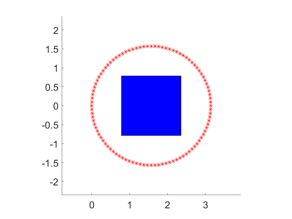
Figure 1: The blue rectangle represents the source support, where ${\rm supp}\,\,f(\cdot,k)=[\pi/4,3\pi/4]$ and ${\rm supp}\,\,g(\cdot)=[-\pi/4,\pi/4]$. The red arsterisks show the measurement points on the circle centered at $(\pi/2,0)$ with radius of $\pi/2$.

Now we provide details of our numerical implementation and delve into a series of experiments carried out in a two-dimensional setting. In our work, we set the lower bound of the wave number as $k_{\min}=0$ and the upper bound as $k_{\max}=K$. Suppose that the function $f(\cdot,k)$ is supported in $[\pi/4,3\pi/4]$ and the function $g(\cdot)$ is supported in $[-\pi/4,\pi/4]$. The radiated field data are collected as follows:

$$\{u(R,\theta_{m},k_{j}):\,\theta_{m}=2\pi m/M,\,k_{j}=jK/J,\,m=1,2,\ldots,M,\,j=1,2,\ldots,J\}.$$ (4.26)

The data is measured on the circle $\partial{\rm B}_{R}(x_{0})$, where $\partial{\rm B}_{R}(x_{0})$ represents the circle centered at $x_{0}=(\pi/2,0)$ with the radius of $R=\pi/2$. Additionally, we calculate the Neumann data by using the formula defined in (4.24) as follows:

$$\{\partial u(R,\theta_{m},k_{j}):\,\theta_{m}=2\pi m/M,\,k_{j}=jK/J,\,m=1,2,\ldots,M,\,j=1,2,\ldots,J\}.$$ (4.27)

Unless otherwise specified, we always set $M=100$ in our experiments. In Fig.1, we show the support of the source $f(x_{1},k)g(x_{2})$ for $k\in[k_{\min},k_{\max}]$ along with the depiction of the measurement boundary $\partial{\rm B}_{R}(x_{0})$. For the sake of simplicity, we assume that $g(x_{2})=1$ if $x_{2}\in[-\pi/4,\pi/4]$ and $g=0$ if else.

4.1 Numerical implementation by the Dirichlet-Laplacian method

In this subsection, by using the expansion defined in (2.12), we reconstruct the exact source $f(\cdot,k)\in L^{2}(0,\pi)$ for some $k\in[0,K]$. To achieve this, one can opt for the eigenfunctions of the Dirichlet Laplacian, as they form a complete and orthonormal set in the space $L^{2}(0,\pi)$. Consider the one-dimensional eigenvalue problem

$$\left\{\begin{array}[]{l}\begin{aligned} -v^{{}^{\prime\prime}}(x_{1})&=\lambda^{2}v(x_{1}),\quad x_{1}\in[0,\pi],\\ v(x_{1})&=0,\qquad\qquad x_{1}=0,\,\pi.\end{aligned}\end{array}\right.$$ (4.29)

We obtain the set of Dirichlet eigenvalues as $\{n^{2},\,|n|\in\mathbb{N}^{+}\}$ and the set of Dirichlet eigenfunctions as $\{\sin(nx_{1}),\,|n|\in\mathbb{N}^{+}\}$. To perform the expansion given in (2.12), we choose a suitably large value of $N$ such that $|n|\leq N$. By substituting the eigenvalues and eigenfunctions calculated from (4.29) into (2.14), i,e, letting $\varphi_{n}=\sin(nx_{1})e^{\sqrt{n^{2}-k^{2}}x_{2}}$ for $|n|\leq N$ in (2.14), we can deduce that

$$\begin{aligned} &\int_{{\rm B}_{R}}f(x_{1},k)g(x_{2})\sin(nx_{1})e^{\sqrt{n^{2}-k^{2}}x_{2}}dx\\ &=\int_{\partial{\rm B}_{R}}\left\{\partial_{\nu}u(x,k)\sin(nx_{1})e^{\sqrt{n^{2}-k^{2}}x_{2}}-u(x,k)\partial_{\nu}\left(\sin(nx_{1})e^{\sqrt{n^{2}-k^{2}}x_{2}}\right)\right\}ds(x).\end{aligned}$$

Note that in our experiments we set $B_{R}=B_{R}(x_{0})$ with $x_{0}=(\pi/2,0)$. It implies that

$$\int_{0}^{\pi}f(x_{1},k_{j})\sin(nx_{1})dx_{1}=\dfrac{M_{n,j}}{G_{n,j}}$$ (4.30)

for $n=\pm 1,\pm 2,\cdots,\pm N$ and $j=1,2,\cdots,J$, where

$$M_{n,j}:=\int_{\partial{\rm B}_{R}}\left\{\partial_{\nu}u(x,k_{j})\sin(nx_{1})e^{\sqrt{n^{2}-k_{j}^{2}}x_{2}}-u(x,k_{j})\partial_{\nu}\left(\sin(nx_{1})e^{\sqrt{n^{2}-k_{j}^{2}}x_{2}}\right)\right\}ds(x),$$

$$G_{n,j}:={\int_{-\frac{\pi}{4}}^{\frac{\pi}{4}}g(x_{2})e^{\sqrt{n^{2}-k_{j}^{2}}x_{2}}dx_{2}}.$$

We approximate $M_{n,j}$ through the discrete measurement data in polar coordinates as defined in (4.26) and (4.27). The reconstructed source $f_{N}(x_{1},k_{j})\sim f(x_{1},k_{j})$ with $x_{1}\in[0,\pi]$ and $k_{j}\in[0,K]$ can be expressed as

$$f_{N}(x_{1},k_{j})=2\sum_{n=1}^{N}\,f_{n,j}\sin(nx_{1}),\quad f_{n,j}=-f_{-n,j},$$ (4.31)

where the coefficients $f_{n,j}$ are approximated by

$$f_{n,j}\approx\dfrac{1}{\pi}\int_{0}^{\pi}f(x_{1},k_{j})\sin(nx_{1})dx_{1}=\dfrac{1}{\pi}\dfrac{M_{n,j}}{G_{n,j}},\quad n=1,2,\cdots,N,\,j=1,2,\cdots,J.$$ (4.32)

It is worthy noting that here we have assumed $G_{n,j}\neq 0$ for all $n=1,2,\cdots,N$ and $j=1,2,\cdots,J$. Similarly, the reconstruction formula using noise data is given by

$$f^{\delta}_{N}(x_{1},k_{j})=2\sum_{n=1}^{N}\,f^{\delta}_{n,j}\sin(nx_{1}),\quad x_{1}\in[0,\pi],\,k_{j}\in[0,K],$$ (4.33)

$$f^{\delta}_{n,j}\approx\dfrac{1}{\pi}\dfrac{M^{\delta}_{n,j}}{G_{n,j}},\quad n=1,2,\cdots,N,\,j=1,2,\cdots,J,$$ (4.34)

where

$$M^{\delta}_{n,j}:=\int_{\partial{\rm B}_{R}}\left\{\partial_{\nu}u^{\delta}(x,k_{j})\sin(nx_{1})e^{\sqrt{n^{2}-k_{j}^{2}}x_{2}}-u^{\delta}(x,k_{j})\partial_{\nu}\left(\sin(nx_{1})e^{\sqrt{n^{2}-k_{j}^{2}}x_{2}}\right)\right\}ds(x).$$

The above reconstruction method is referred to as the Dirichlet-Laplacian method.

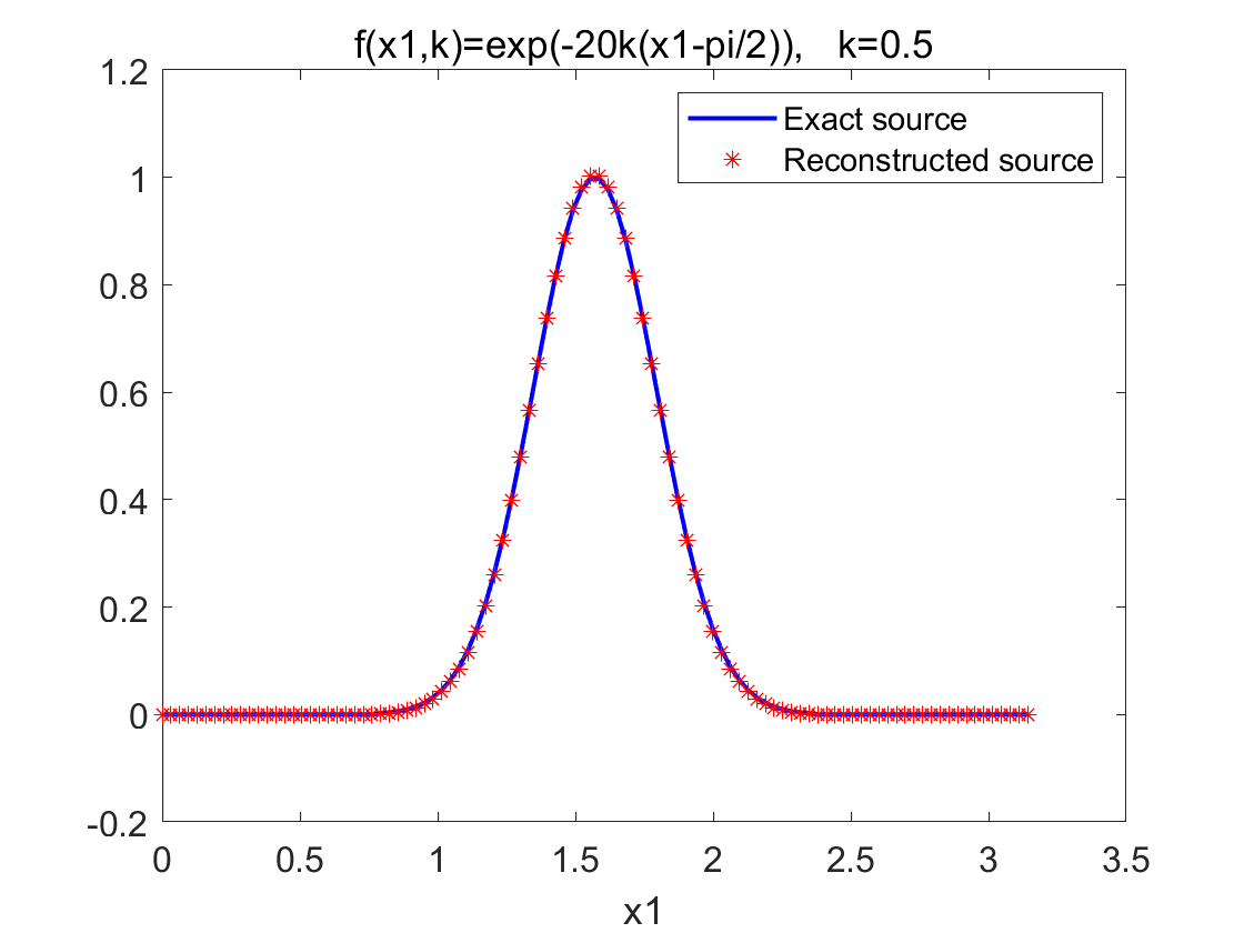
(a) $f_{1}(x_{1},k)$, $k=0.5$, $N=17$

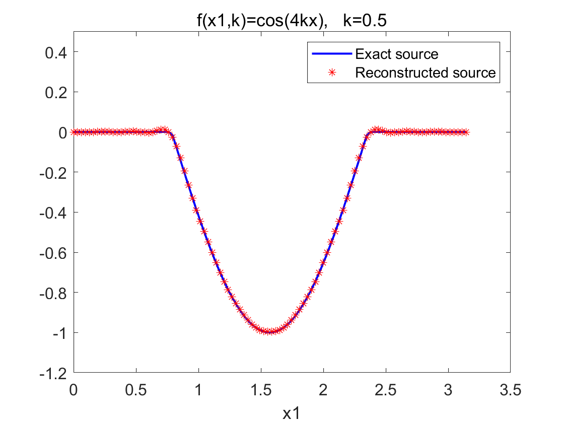
(b) $f_{2}(x_{1},k)$, $k=0.5$, $N=25$

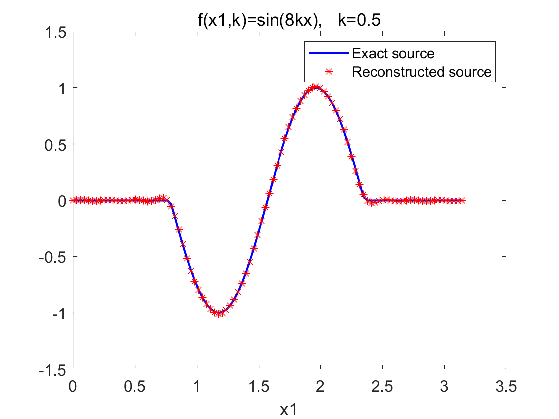
(c) $f_{3}(x_{1},k)$, $k=0.5$, $N=26$

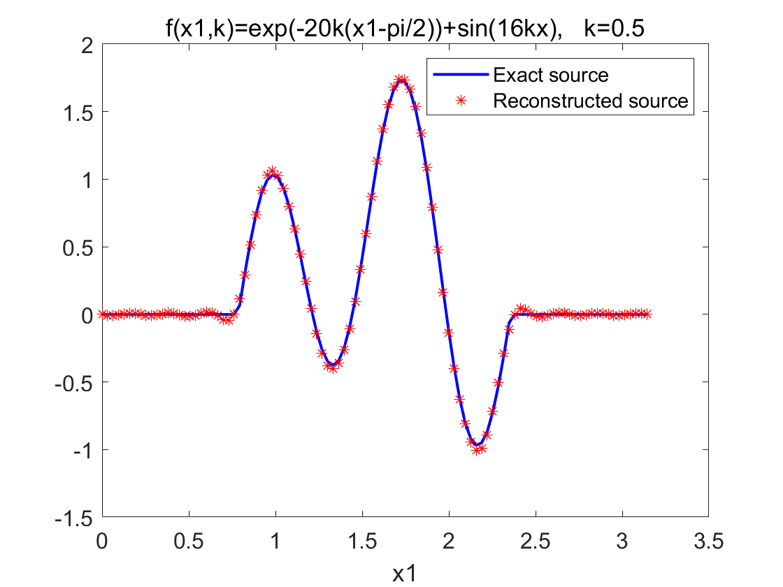
(d) $f_{4}(x_{1},k)$, $k=0.5$, $N=26$

Figure 2: The reconstructed source by the Dirichlet- Laplacian method with a fix $k=0.5$. The four source functions $f_{j}(x_{1},k)$ ($j=1,2,3,4$) shown in (a)-(d) are reconstructed with $N=17,\,25,\,26,\,26$, respectively.

Using formulas (4.31) and (4.32), we demonstrate the reconstructions of the following source functions when $k=0.5$:

$$f_{1}(x_{1},k)=\left\{\begin{array}[]{l}e^{-20k(x_{1}-\pi/2)^{2}},\quad x_{1}\in[\frac{\pi}{4},\frac{3\pi}{4}],\\ 0,\qquad\qquad\qquad\quad{\rm otherwise},\end{array}\right.$$ (4.37)

$$f_{2}(x_{1},k)=\left\{\begin{array}[]{l}\cos(4kx_{1}),\quad x_{1}\in[\frac{\pi}{4},\frac{3\pi}{4}],\\ 0,\qquad\qquad\quad{\rm otherwise},\end{array}\right.$$ (4.40)

$$f_{3}(x_{1},k)=\left\{\begin{array}[]{l}\sin(8kx_{1}),\quad x_{1}\in[\frac{\pi}{4},\frac{3\pi}{4}],\\ 0,\qquad\qquad\quad{\rm otherwise},\end{array}\right.$$

$$f_{4}(x_{1},k)=\left\{\begin{array}[]{l}e^{-20k(x_{1}-\pi/2)^{2}}+\sin(8kx_{1}),\quad x_{1}\in[\frac{\pi}{4},\frac{3\pi}{4}],\\ 0,\qquad\qquad\qquad\qquad\qquad\qquad{\rm otherwise}.\end{array}\right.$$

It is obvious that the source can be well reconstructed by choosing an appropriate parameter $N$ in Fig.2. We use the source function $f_{1}(x_{1},0.5)$ to generate the noise-free radiation field data on $\partial{\rm B}_{R}$. The reconstructed source $f_{N}(x_{1},0.5)$ is displayed in Fig.2 (a) with $N=17$. In Fig.2 (b), the source function $f_{2}(x_{1},0.5)$ can be well reconstructed with $N=25$. Choosing the source function $f_{3}$ or $f_{4}$ with $k=0.5$, we obtain the reconstruction results in Fig.2 (c) and Fig.2 (d) with $N=26$, respectively.

However, the above method fails in the case $G_{n,j}=0$, because the denominator on the right side of (4.32) vanishes. For example, in reconstructing the source function $f_{1}(x_{1},k)$ with $k=1$, or the source function

$$f_{5}(x_{1},k)=\left\{\begin{array}[]{l}\cos(2/3kx_{1}),\quad x_{1}\in[\frac{\pi}{4},\frac{3\pi}{4}],\\ 0,\qquad\qquad\qquad{\rm otherwise},\end{array}\right.$$

with $k=3$, one cannot obtain a correct reconstruction with $N=10$.

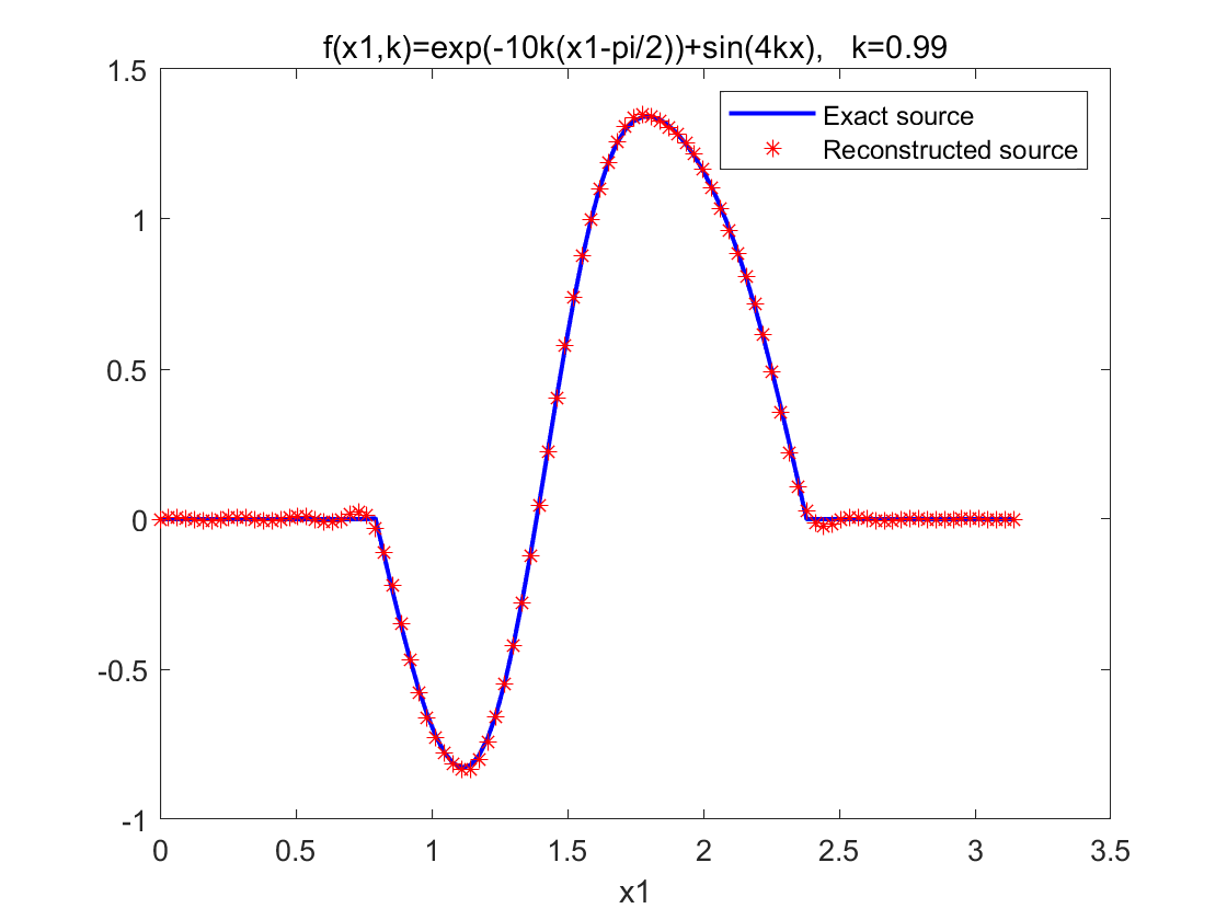
(a) $k_{1}=0.99$

(b) $k_{2}=1.99$

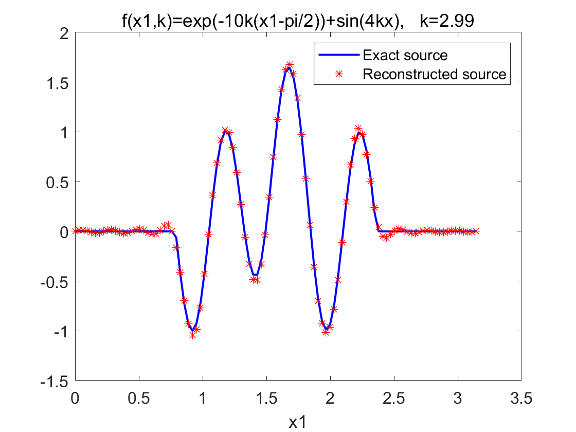
(c) $k_{3}=2.99$

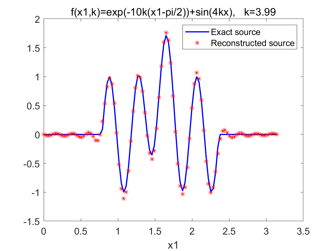
(d) $k_{4}=3.99$

Figure 3: The reconstructed results for the source function $x_{1}\mapsto e^{-10k_{j}(x_{1}-\pi/2)^{2}}+\sin(4k_{j}x_{1})$ supported in $[\pi/4,3\pi/4]$ and $N=26$ by the Dirichlet-Laplacian method. Here we use four different wave-numbers $k_{1}=0.99$, $k_{2}=1.99$, $k_{3}=2.99$ and $k_{4}=3.99$.

Next, we choose different wave-numbers $0<k\notin\mathbb{N}^{+}$ to test the effectiveness of the Dirichlet-Laplacian method. Fig.3 illustrates that the source function $e^{-10k(x_{1}-\pi/2)^{2}}+\sin(4kx_{1})$, supported in $[\pi/4,3\pi/4]$, can be well reconstructed for various wave-numbers $0<k\notin\mathbb{N}^{+}$. When $k_{1}=0.99$ and $N=26$ (as shown in Fig. 3 (a)), it is evident that the reconstructed source closely matches the exact source. In other cases, such as $k_{2}=1.99$, $k_{3}=2.99$ and $k_{4}=3.99$, we also achieve satisfactory reconstructions with $N=26$.

Finally, we examine the sensitivity of the Dirichlet-Laplacain method to random noise. The measurement data (4.23) is polluted by random noise using the formula (4.25). Fig.4 displays the reconstructions $f_{N}^{\delta}$ of the source function $f=\sin(8kx_{1})$, supported in $[\pi/4,3\pi/4]$, with noise levels $\delta=0.5\%$, $\delta=2\%$, $\delta=10\%$ and $\delta=30\%$. It can be concluded that the error decreases as the noise level decreases, where the error is defined as

$${\rm error}=\dfrac{\|f-f_{N}^{\delta}\|_{2}}{\|f\|_{2}}.$$ (4.44)

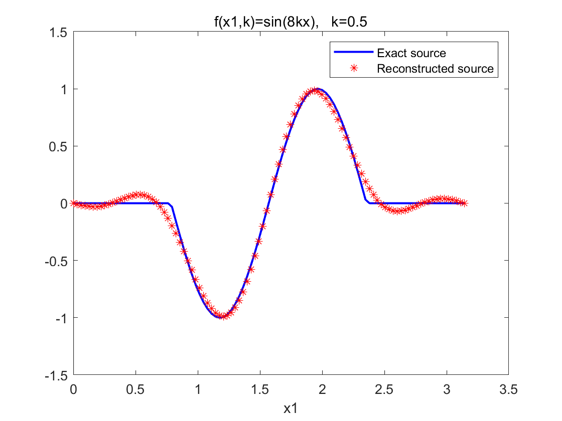
(a) $\delta=0.5\%$, $N=6$, ${\rm error}=0.1015$

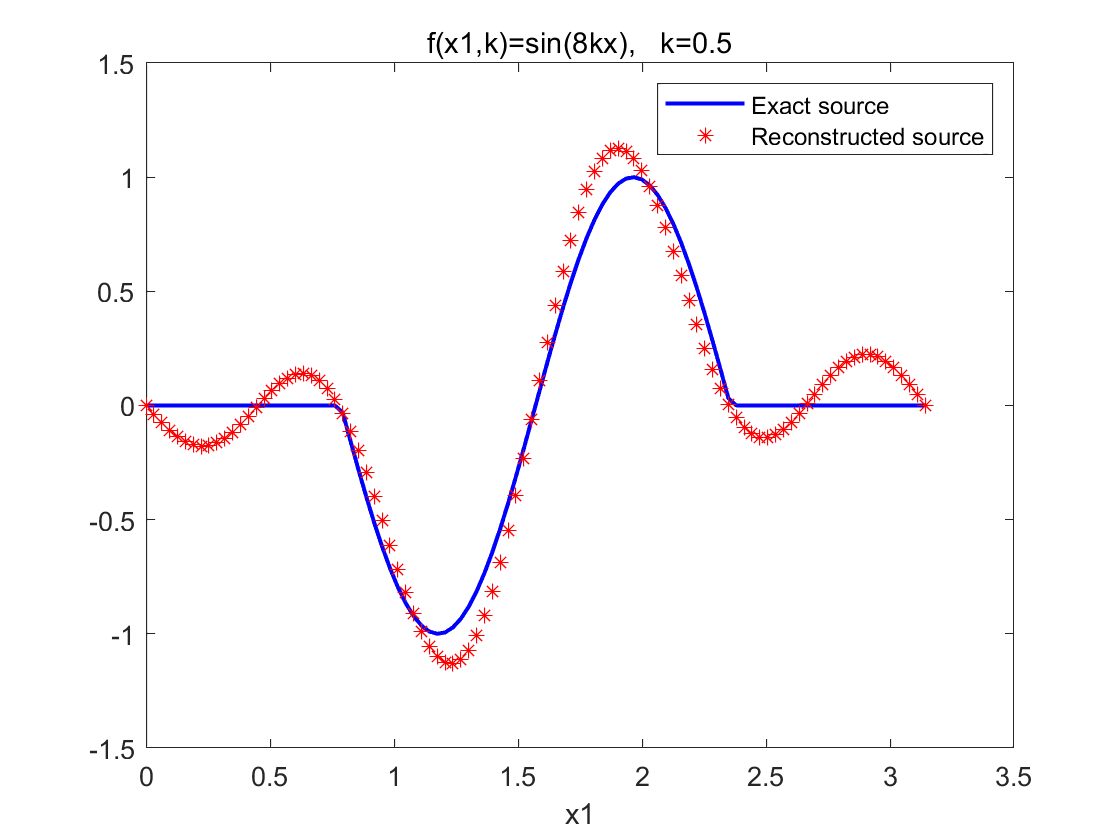
(b) $\delta=2\%$, $N=6$, ${\rm error}=0.2226$

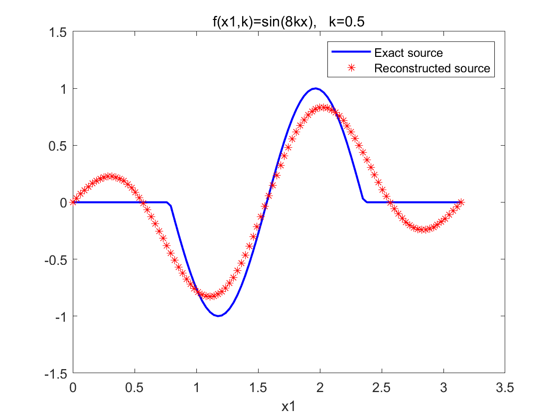
(c) $\delta=10\%$, $N=4$, ${\rm error}=0.3739$

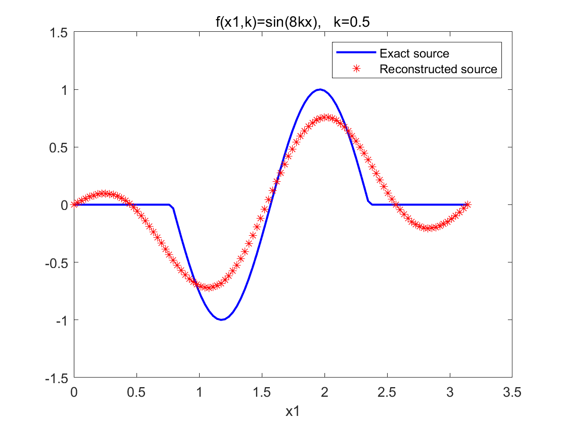
(d) $\delta=30\%$, $N=4$, ${\rm error}=0.4383$

Figure 4: The reconstructed source by the Dirichlet-Laplacian method with different noise levels $\delta$.

4.2 Numerical Implementation by the Fourier-Transform Method

The purpose of this subsection is to reconstruct the exact source $f(\cdot,k)\in L^{2}(0,\pi)$ for some $k\in[0,K]$ by using the Fourier expansion. A computational formula for each Fourier coefficient is also established. We still cosider the source function considered as in Fig.1. According to (2.9), the Fourier basis functions in $L^{2}[0,\pi]$ are given by

$$e^{i\xi_{1}x_{1}},\quad\xi_{1}^{2}+\xi_{2}^{2}=k^{2},\,k\in[0,K],$$

where $\xi_{1}=2n$, $n\in\mathbb{Z}$, since $\xi_{1}=\frac{2\pi}{2R}n=2n$ by our choice $R=\pi/2$. Next, we establish computational formulas for the Fourier coefficients of $f(x_{1},k)\in L^{2}[0,\pi]$ under the Fourier basis functions $\{e^{i(2n)x_{1}}:x_{1}\in[0,\pi],\,n\in\mathbb{Z}\}$. According to formula (2.10), we obtain

$$\begin{aligned} &\int_{{\rm B}_{R}}f(x_{1},k)g(x_{2})e^{-i(\xi_{1}x_{1}+\xi_{2}x_{2})}dx\\ &=\int_{\partial{\rm B}_{R}}\{\partial_{\nu}u(x,k)+i\xi\cdot\nu u(x,k)\}e^{-i(\xi_{1}x_{1}+\xi_{2}x_{2})}ds(x).\end{aligned}$$

A simple calculation yields that

$$\int_{0}^{\pi}f(x_{1},k_{j})e^{-i(2n)x_{1}}dx_{1}=\dfrac{\tilde{M}_{n,j}}{\tilde{G}_{n,j}}$$ (4.45)

for $n\in\mathbb{Z}$, $j=1,2,\cdots,W$, where $\tilde{M}_{n,j}$ and $\tilde{G}_{n,j}$ are defined as

$$\tilde{M}_{n,j}:=\int_{\partial{\rm B}_{R}}\{\partial_{\nu}u(x,k_{j})+i(2n,\sqrt{k_{j}^{2}-4n^{2}})\cdot\nu u(x,k_{j})\}e^{-i(2nx_{1}+\sqrt{k_{j}^{2}-4n^{2}}x_{2})}ds(x),$$

$$\tilde{G}_{n,j}:={\int_{-\frac{\pi}{4}}^{\frac{\pi}{4}}g(x_{2})e^{-i\sqrt{k_{j}^{2}-4n^{2}}x_{2}}dx_{2}}.$$

The reconstructed source $\tilde{f}_{N}(x_{1},k_{j})$ with $x_{1}\in[0,\pi]$, $k_{j}\in[0,K]$ can be written as

$$\tilde{f}_{N}(x_{1},k_{j})=\sum_{\left|n\right|\leq N}\,\tilde{f}_{n,j}e^{i(2n)x_{1}}.$$ (4.46)

From (4.45), the coefficients are approximately computed by

$$\tilde{f}_{n,j}\approx\dfrac{1}{\pi}\int_{0}^{\pi}f(x_{1},k_{j})e^{-i(2n)x_{1}}dx_{1}=\dfrac{1}{\pi}\dfrac{\tilde{M}_{n,j}}{\tilde{G}_{n,j}},\quad n\in\mathbb{Z},\,j=1,2,\cdots,J,$$ (4.47)

where the denominator is again assumed to be non-vanishing. Similarly, the reconstruction formula from noise data is given by

$$\tilde{f}^{\delta}_{N}(x_{1},k_{j})=\sum_{\left|n\right|\leq N}\,\tilde{f}_{n,j}e^{i(2n)x_{1}},\quad x_{1}\in[0,\pi],\,k_{j}\in[0,K],$$

$$\tilde{f}^{\delta}_{n,j}\approx\dfrac{1}{\pi}\dfrac{\tilde{M}^{\delta}_{n,j}}{\tilde{G}_{n,j}},\quad n\in\mathbb{Z},\,j=1,2,\cdots,W,$$

where

$$\tilde{M}^{\delta}_{n,j}:=\int_{\partial{\rm B}_{R}}\{\partial_{\nu}u^{\delta}(x,k_{j})+i(2n,\sqrt{k_{j}^{2}-4n^{2}})\cdot\nu u^{\delta}(x,k_{j})\}e^{-i(2nx_{1}+\sqrt{k_{j}^{2}-4n^{2}}x_{2})}ds(x).$$

These reconstruction formulas are quite similar to the Dirichlet-Laplacian method.

Using formulas (4.46) and (4.47), we present the reconstructions when $k=0.5$. Choosing the source function $f_{1}(x_{1},k)$ as in (4.37), the reconstructed results are shown in Fig.5 (a) with $N=9$. In Fig.5 (b), the source function $f_{2}(x_{1},k)$, identical to $\eqref{equ:f2}$, is well reconstructed with $N=12$ and $k=0.5$. For source functions $\cos(12kx_{1})$ supported in $[\pi/4,3\pi/4]$ with $k=0.5$ and $e^{-20k(x_{1}-\pi/2)^{2}}+\cos(12kx_{1})$ supported in $[\pi/4,3\pi/4]$ with $k=0.5$, the experimental results shown in Fig.5 (c) with $N=12$ and Fig.2 (d) with $N=12$ demonstrate that the reconstructed sources closely resemble the exact one.

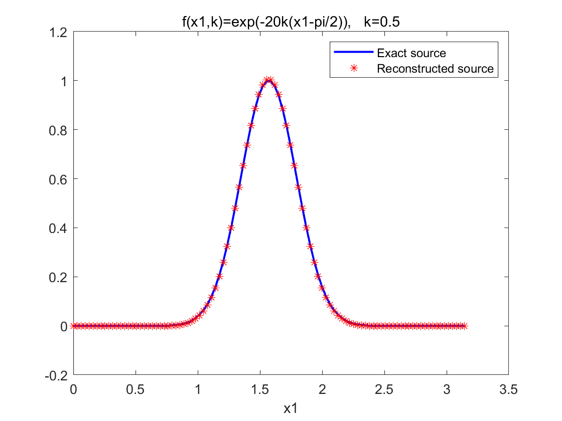
(a) $e^{-20k(x_{1}-\pi/2)^{2}}$, $N=9$

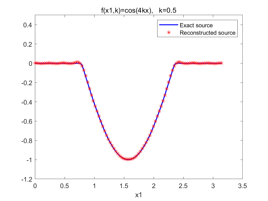
(b) $\cos(4kx_{1})$, $N=12$

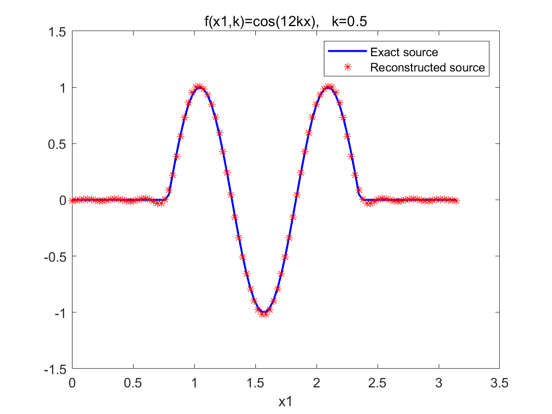
(c) $\cos(12kx_{1})$, $N=12$

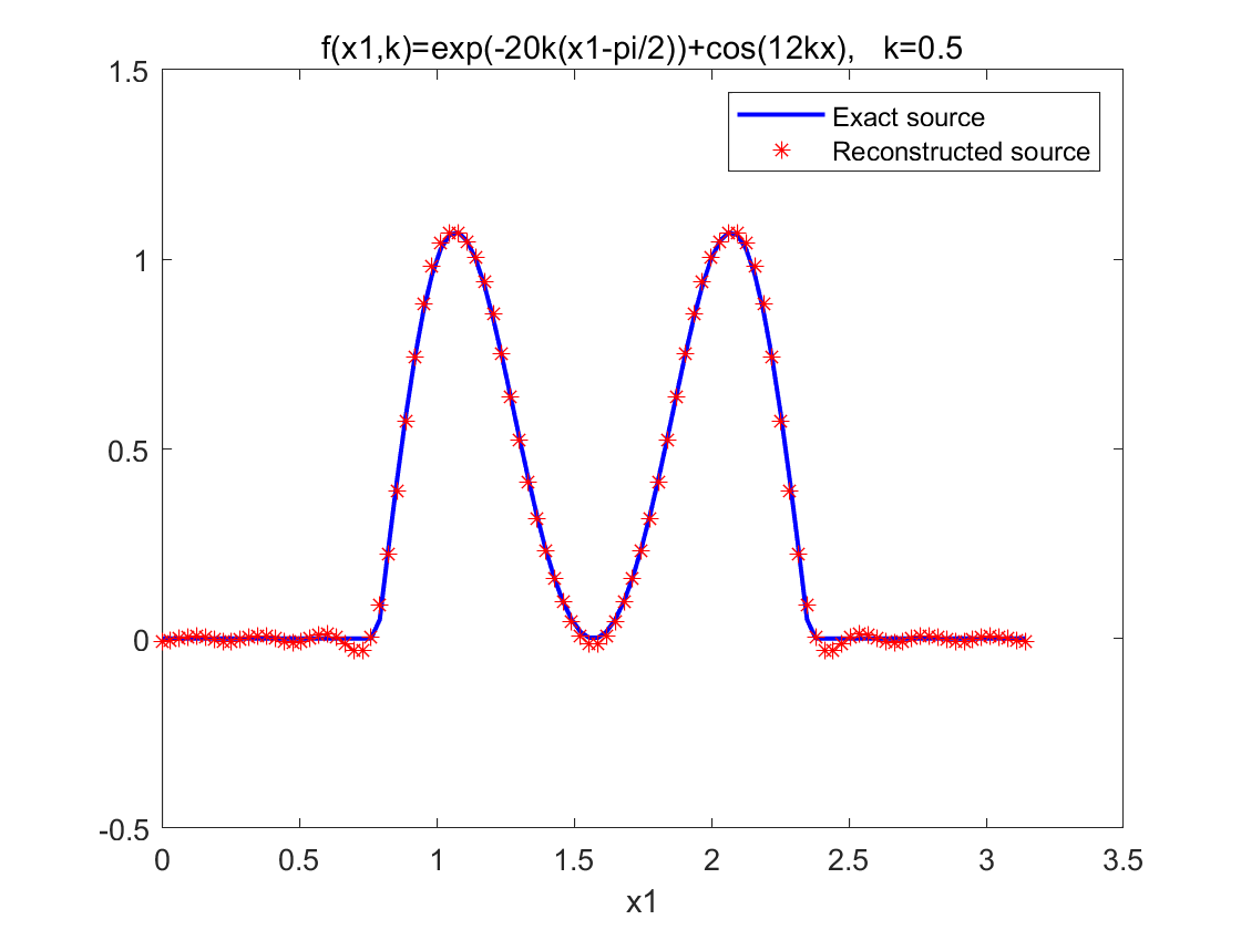
(d) $e^{-20k(x_{1}-\pi/2)^{2}}+\cos(12kx_{1})$, $N=12$

Figure 5: The reconstructed source by the Fourier-Transform method with $k=0.5$. Four different sources are reconstructed with $N=9,\,12,\,12,\,12$, respectively.

It is important to note that for $k=2n$, $n\in\mathbb{N}^{+}$, the source function cannot be reconstructed due to the vanishing of $\tilde{G}_{n,j}$. However, by approximating such wave-numbers $k=2n$ with $k=2n\pm\varepsilon$, $0<\varepsilon\ll 1$, $n\in\mathbb{N}^{+}$, Fig. 6 (b) displays a successful reconstruction of $\cos(kx_{1})$ supported in $[\pi/4,3\pi/4]$ with $k=2$. Following this, we apply the Fourier-Transform method to the source $e^{-5k(x_{1}-\pi/2)^{2}}$ by using different wave numbers. The recovery results are presented in Fig.7. The recreated image in Fig.7(a) closely resembles the exact source function with $k=1.5$ and $N=8$. In Fig.7(b), employing $k=3.5$ and $N=8$ for the source reconstruction yields favorable results. Subsequently, Fig.7 (c) and Fig.7 (d) display the reconstructed sources with $k=5.5$, $N=13$ and $k=7.5$, $N=13$, respectively. It is evident from these figures that as the wave number $k$ increases, the recovery effect becomes slightly less accurate.

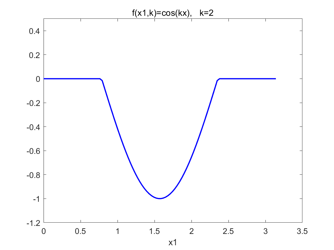
(a) $\cos(kx_{1})$, $k=2$, $N=12$

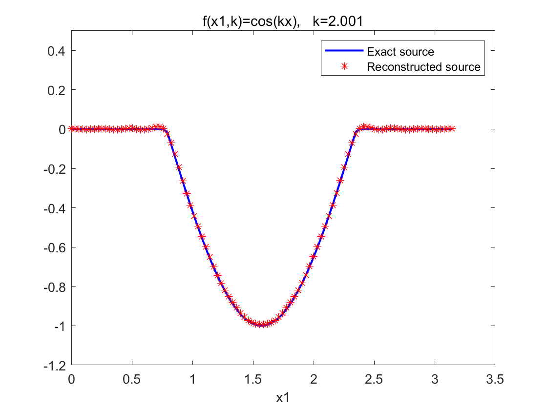
(b) $\cos(kx_{1})$, $k=2.001$, $N=12$

Figure 6: The reconstructed source by the Fourier-Transform method with $N=12$. The left shows the exact source function with $k=2$, while the right shows the reconstruction result with $k=2.001$.

At the end, we investigate the impact of noise on the Fourier-Transform method. The measurement data (4.23) is polluted by random noise using the formula (4.25). Different noise levels, $\delta=0.5\%$, $\delta=2\%$, $\delta=10\%$ and $\delta=20\%$, are introduced. Fig.8 illustrates the recreated results, indicating that the reconstruction error decreases as the noise level decreases, where the error is again defined as (4.44).

5 Conclusion

In this research, we have established uniqueness, increasing stability and algorithms for an inverse wave-number-dependent source problem. In $d$-dimensions, the unknown source function depends on $\tilde{x}=(x_{1},\cdots,x_{d-1})$ and $k$ but independent of $x_{d}$. The Fourier-Transform method, grounded in the Fourier basis, ensures both uniqueness and stability. Conversely, the Dirichlet-Laplacian method is constructed using Dirichlet-Laplacian eigenfunctions, though its stability remains to be futher examined. Two efficient non-iterative numerical algorithms have been developed. A possible continuation of this work is to investigate the stability under incomplete data and explore scenarios involving other kinds of wave-number-dependent sources.

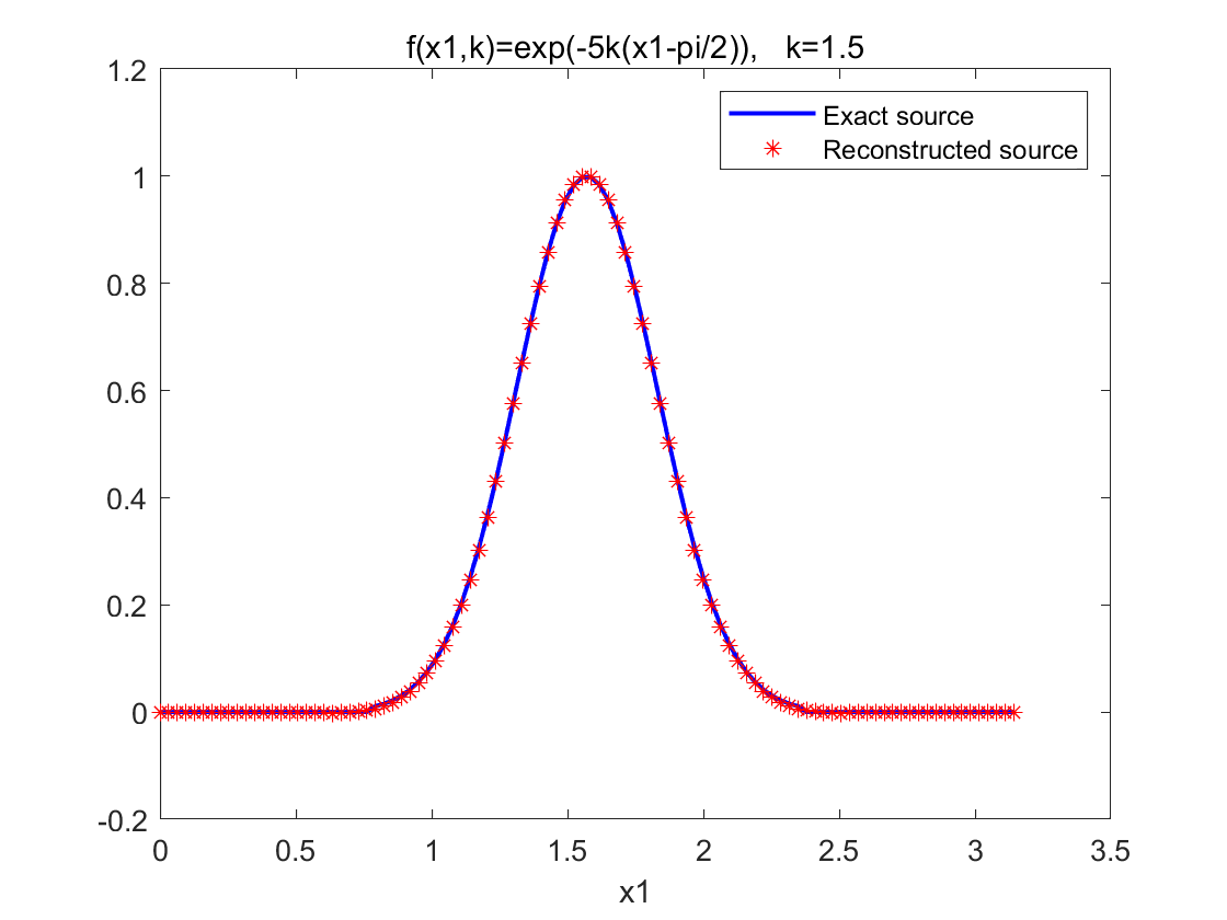
(a) $k=1.5$, $N=8$

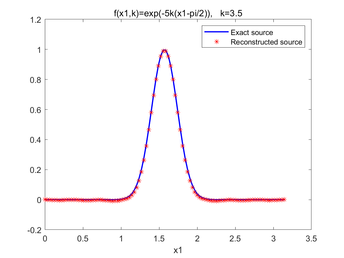
(b) $k=3.5$, $N=8$

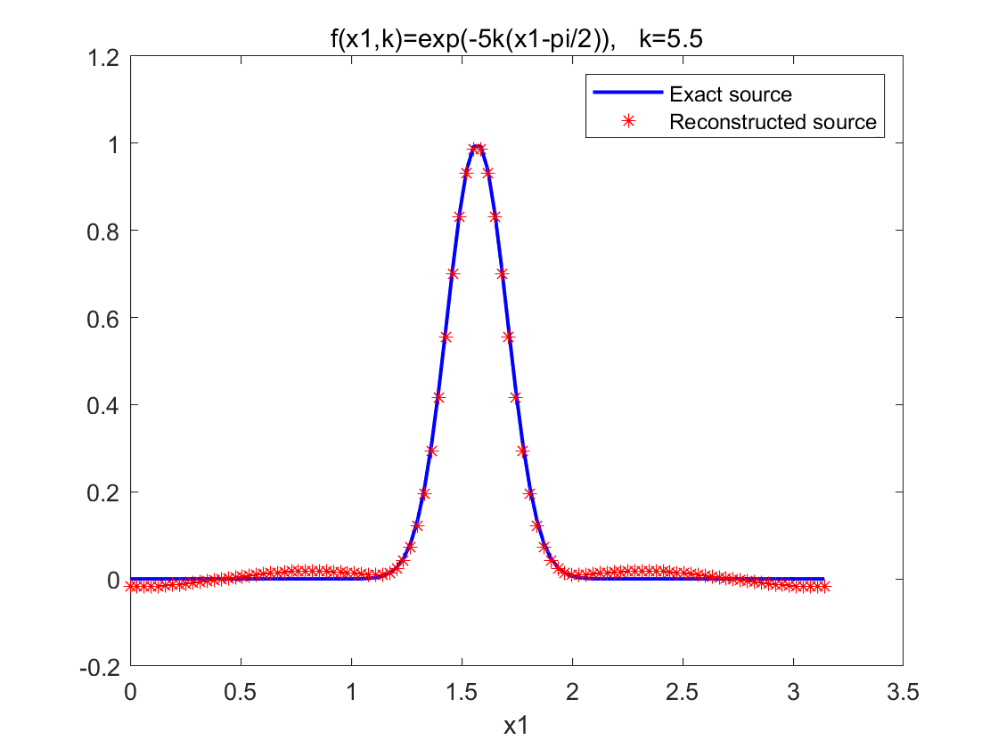
(c) $k=5.5$, $N=13$

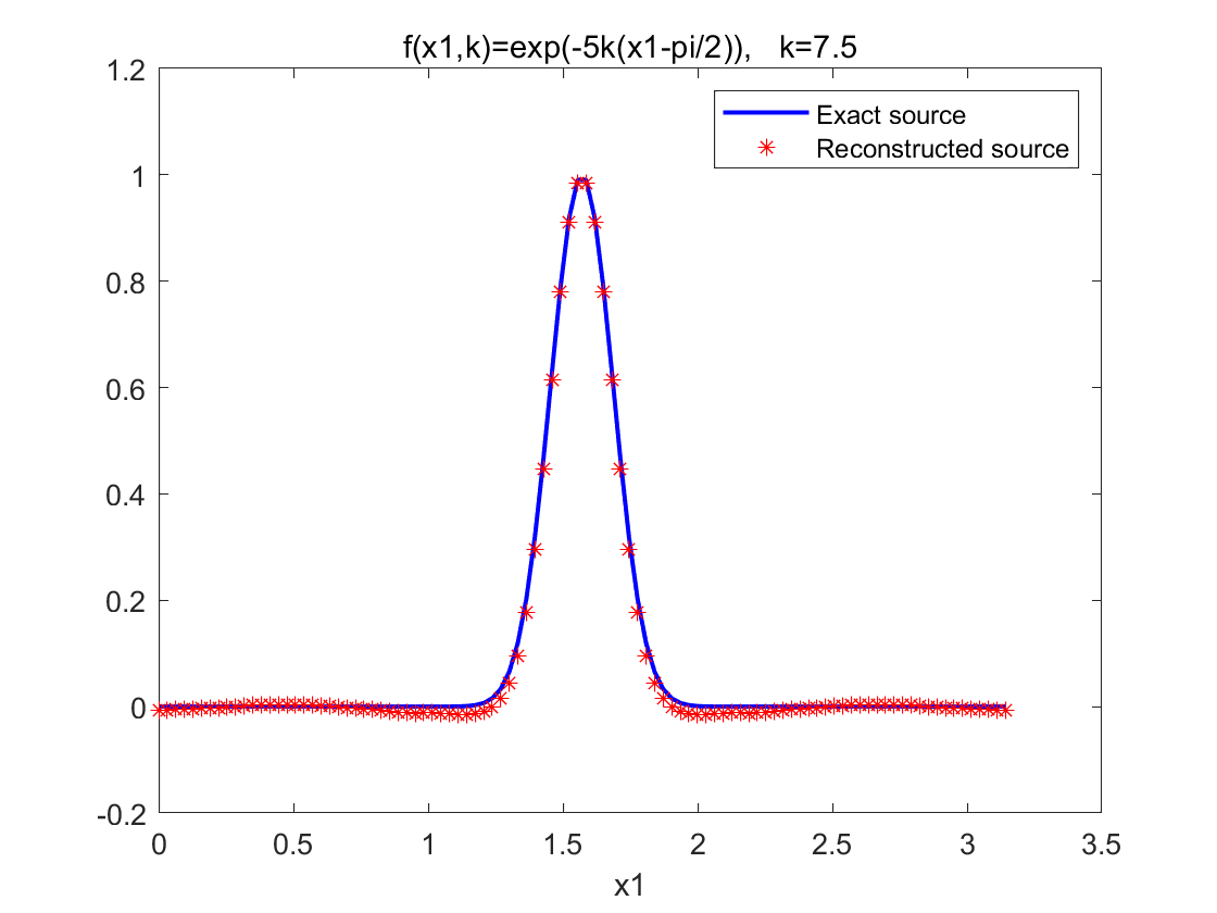
(d) $k=7.5$, $N=13$

Figure 7: The reconstructed source using the Fourier-Transform method for the given source $e^{-5k(x_{1}-\pi/2)^{2}}$. Each figure corresponds to a different value of $k$.

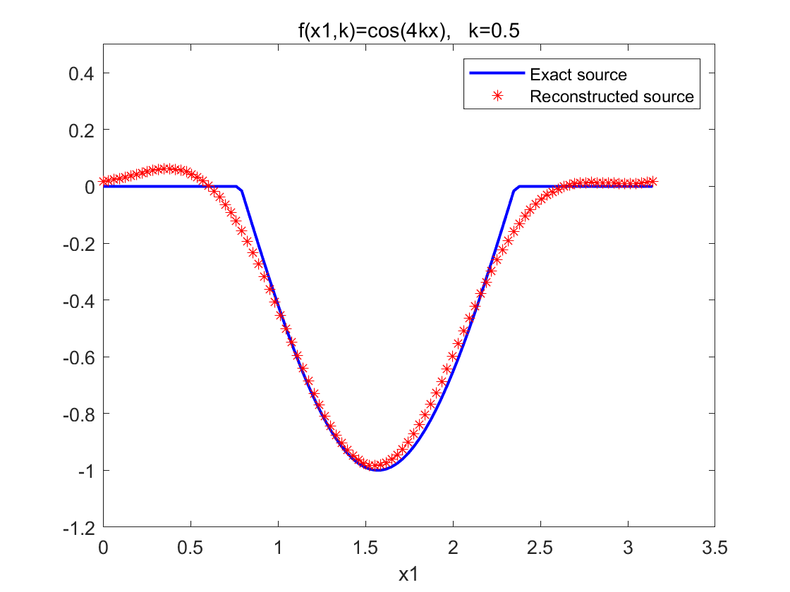
(a) $\delta=0.5\%$, $N=2$, ${\rm error=0.0965}$

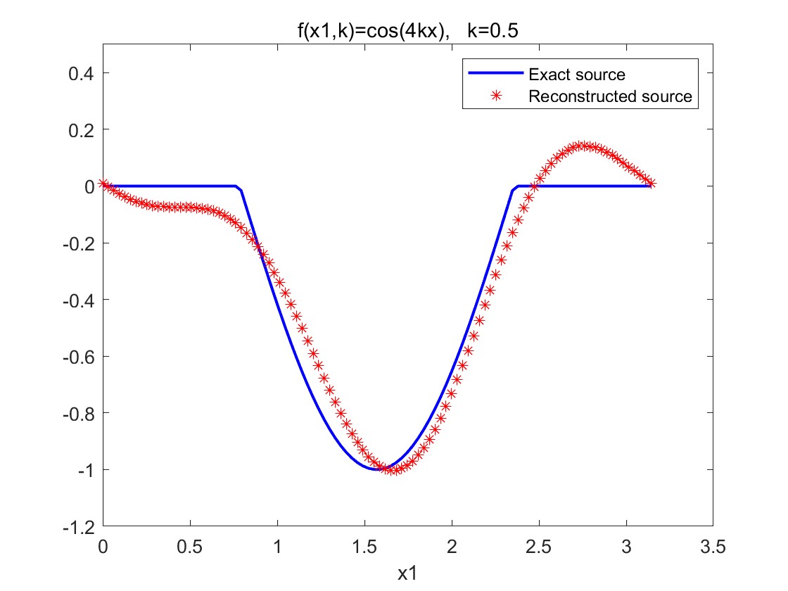
(b) $\delta=2\%$, $N=2$, ${\rm error=0.1637}$

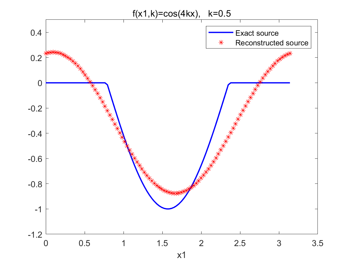
(c) $\delta=10\%$, $N=1$, ${\rm error=0.3516}$

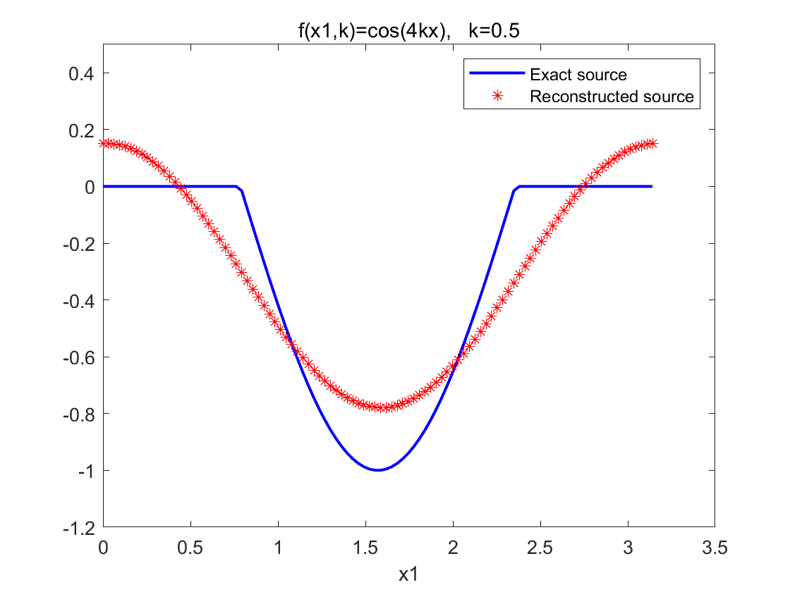
(d) $\delta=20\%$, $N=1$, ${\rm error=0.4106}$

Figure 8: The reconstructed sources using the Fourier-Transform method with different noise levels $\delta$.

References

- [1] S. Acosta, S. Chow, J. Taylor and V. Villamizar, On the multi-frequency inverse source problem in heterogeneous media, Inverse Problems, 28 (2012),075013.
- [2] A. Alzaalig, G. Hu, X. Liu and J. Sun, Fast acoustic source imaging using multi-frequency sparse data, Inverse problems, 36 (2020), 025009.
- [3] G. Arfken, H. Weber and F. Harris, Mathematical Methods for Physicists (Seventh Edition), Academic Press, 2013, 75–79.
- [4] S. Arridge, Optical tomography in medical imaging, Inverse Problems, 15 (1999), 41–93.
- [5] G. Bao, P. Li and J. Lin, Inverse scattering problems with multi-frequencies, Inverse Problems, 31(2015), 093001.
- [6] G. Bao, J. Lin and F. Triki, A multi-frequency inverse source problem, J. Differential Equations, 249 (2010), 3443–3465.
- [7] G. Bao, S. Lu, W. Rundell and B. Xu, A recursive algorithm for multi-frequency acoustic inverse source problems, SIAM J. Numer. Anal., 53 (2015), 1608-1628.
- [8] G. Bao, Y. Liu and F. Triki, Recovering point sources for the inhomogeneous Helmholtz equation, Inverse problems, 37 (2021), 095005.
- [9] M. Bellassoued and M. Yamamoto, Carleman estimates and applications to inverse problems for hyperbolic systems, Springer Japan, Tokyo, (2017).
- [10] M. Bellassoued and I. Ben Aicha, Stable determination outside a cloaking region of two time-dependent coefficients in an hyperbolic equation from Dirichlet to Neumann map, J. Math. Anal. Appl., 229 (2017), 46–76.
- [11] N. Bleistein and J. Cohen, Nonuniqueness in the inverse source problem in acoustics and electromagnetics, J. Math. Phys., 18 (1977), 194-201.
- [12] J. Cheng, V. Isakov and S. Lu, Increasing stability in the inverse source problem with many frequencies, J. Differential Equations, 260 (2017), 4786–4804.
- [13] A.P. Choudhury and H. Heck, Increasing stability for the inverse problem for the Schrödinger equation, Math. Methods Appl. Sci., 41 (2018), 606-614.
- [14] M. Eller and N. Valdivia, Acoustic source identification using multiple frequency information, Inverse Problems, 25 (2009), 115005.
- [15] M. Entekhabi, Increasing stability in the two dimensional inverse source scattering problem with attenuation and many frequencies, Inverse Problems, 34 (2018), 115001.
- [16] M. Entekhabi, V. Isakov, Increasing stability in acoustic and elastic inverse source problems, SIAM J. Math. Anal., 52 (2020),5232-5256.
- [17] A. Fokas, Y. Kurylev and V. Marinakis, The unique determination of neuronal currents in the brain via magnetoencephalography, Inverse Problems, 20 (2015), 1067–1082.
- [18] H. Guo and G. Hu, Inverse wave-number-dependent source problems for the Helmholtz equation, arXiv:2305.07459.
- [19] H. Guo, G. Hu and M. Zhao, Direct sampling method to inverse wave-number-dependent source problems: determination of the support of a stationary source, Inverse Problems 39 (2023), 105008.
- [20] B. Harrison, An inverse problem in underwater acoustic source localization: robust matched-field processing, Inverse Problems, 16 (2000), 1641.
- [21] G. Hu and Y. Kian, Uniqueness and stability for the recovery of a time-dependent source and initial conditions in elastodynamics, Inverse Probl. Imaging., 14 (2020), 463–487.
- [22] G. Hu, Y. Kian and Y. Zhao, Uniqueness to some inverse source problems for the wave equation in unbounded domains, Acta Math. Appl. Sin. Engl. Ser, 36 (2020), 463–487.
- [23] V. Isakov and S. Lu, Inverse source problems without (pseudo) convexity assumptions, Inverse Problems Imag, 12 (2018), 955–970.
- [24] V. Isakov, Increasing stability in the continuation for the Helmholtz equation with variable coefficient, Comtemp. Math., 426 (2007), 255-269.
- [25] V. Isakov, Inverse Problems for Partial Differential Equations, Springer, New York, 2017.
- [26] V. Isakov, S. Nagayasu, G. Uhlmann and J-N. Wang, Increasing stability of the inverse boundary value problem for the Schrödinger equation, Contemp. math., 615 (2014), 131-141.
- [27] P. Li and G. Yuan, Increasing stability for the inverse source scattering problem with multi-frequencies, Inverse problems and Imaging, 11 (2017), 745–759.
- [28] P. Li, J. Zhai and Y. Zhao, Stability for the acoustic inverse source problem in inhomogeneous media, SIAM J. Appl. Math., 80 (2020), 2547–2559.
- [29] W. McLean, Strongly elliptic systems and boundary integral equations, Cambridge university press, 2000, 288–289.
- [30] P. Stefanov and G. Uhlmann, Themoacoustic tomography arising in brain imaging, Inverse Problems, 27 (2011), 075011.
- [31] D. Zhang and Y. Guo, Fourier method for solving the multi-frequency inverse source problem for the Helmholtz equation, Inverse Problems, 36 (2020), 463–487.