Inexact Restoration via random models for unconstrained noisy optimization

Abstract.

We study the Inexact Restoration framework with random models for minimizing functions whose evaluation is subject to errors. We propose a constrained formulation that includes well-known stochastic problems and an algorithm applicable when the evaluation of both the function and its gradient is random and a specified accuracy of such evaluations is guaranteed with sufficiently high probability. The proposed algorithm combines the Inexact Restoration framework with a trust-region methodology based on random first-order models. We analyse the properties of the algorithm and provide the expected number of iterations performed to reach an approximate first-order optimality point. Numerical experiments show that the proposed algorithm compares well with a state-of-the-art competitor.

1. Introduction

We consider unconstrained optimization problems of the form

(1.1) $$\min_{x\in\mathbb{R}^{n}}f(x),$$

where $f:\mathbb{R}^{n}\rightarrow\mathbb{R}$ is a smooth function whose evaluation is inexact. In particular, we consider problems where the evaluation of both the objective function and its gradient is random and sufficient accuracy in the estimates can be guaranteed with sufficiently high probability [17, 23]. This class of problems include the minimization of either functions which are intrinsically noisy or expensive functions which are approximately computed, see e.g., [8, 15, 16].

Our proposal for the numerical solution of such problem is based on the Inexact Restoration framework for constrained optimization problems proposed in [22]. Inexact Restoration is typically a two-phase method consisting of a restoration phase and an optimization phase; the restoration phase improves feasibility and does not call for function evaluations while the optimization phase improves the objective function value with respect to the point obtained in the restoration phase, see e.g., [1, 9, 11, 18]. Such a framework has been successfully employed in the minimization of functions whose computation is intrinsically inexact; specifically, the exact evaluation of the function is interpreted as feasibility of a constrained problem and the restoration phase increases the accuracy in the function evaluation [19, 12, 13, 14]. Analogously, Inexact Restoration has been fruitfully applied in finite-sum minimization with inexact functions and derivatives [5, 4, 6].

In order to apply the Inexact Restoration approach, we reformulate (1.1) as

(1.2) $$\min_{x\in\mathbb{R}^{n}}\bar{f}(x,y)\quad\mbox{ subject to }h(y)=0,$$

where $\bar{f}(x,y)$ is an estimate of $f(x)$ with noise level $y$, $h:Y\rightarrow\mathbb{R}$ is a non-negative function such that the lower $h(y)$ is, the higher the accuracy of the function and gradient estimates is in probability and $h(y)=0$ represents the ideal case where the function and the gradient are evaluated exactly. We show that our problem setting is viable for well-known optimization problems and then design and analyze a new trust-region algorithm that employs random first-order models for optimization. We borrow ideas from the Inexact Restoration approach and adapt such framework, in order to define an algorithm that is well-defined and theoretically well founded even if the random models are inaccurate at some iterations. We denote our algorithm as irerm (Inexact REstoration with Random Models).

Our work is different from existing works on the Inexact Restoration approach for the minimization of noisy functions [10, 19, 12, 14], where either the noise is controllable in a deterministic way or the noise is stochastic but the probability of obtaining sufficiently accurate estimates of functions and gradients is increasing; by contrast, we assume that the noise is stochastic and the probability of obtaining accurate estimates is prefixed. A stochastic first-order trust-region algorithm with Inexact Restoration has been proposed in [4], but only for finite-sum minimization problems; by contrast, irerm can be applied to any unconstrained differentiable problem of the form (1.1). Our algorithm falls in the class of trust-region procedures with random models, see e.g., the contributions [2, 3, 7, 16, 20]. With respect to the existing literature, irerm is inspired by storm, the trust-region algorithm with random models proposed in [16] and further analysed in [7]. Differently from storm, the probabilistic accuracy requirements on function and gradient estimates are explicitly imposed within irerm using problem (1.2) and a suitable function $h$. Furthermore, the acceptance test in irerm is a stochastic counterpart of the rule typically adopted in the Inexact Restoration framework and involves both $h$ and the noisy function $\bar{f}$, whereas the acceptance test in storm is a stochastic counterpart of the classical trust-region acceptance test and involves only the noisy values of $f$.

We design the new algorithm irerm and show that it shares theoretical properties analogous to those of storm. Particularly, we provide a bound on the expected number of iterations needed to achieve a certain accuracy in the norm of the true gradient. Furthermore, we compare numerically irerm with storm on a collection of least-squares problems and observe that irerm achieve comparable or lower noiseless values of $f$ than storm.

The rest of the paper is organized as follows. In Section 2 we discuss our constrained problem formulation (1.2) and present fields of applications for our approach. In Section 3 we introduce our procedure and in Section 4 we study its theoretical properties and provide the expected number of iterations performed to reach an approximate first-order optimality point for (1.1). Finally, in Section 5 we provide the numerical validation of our new algorithm.

2. Problem formulation

In this section, we discuss the assumptions made on problem (1.1) and its constrained formulation (1.2) and show that they are viable.

Let $\bar{f}(x,y)$ and $\nabla_{x}\bar{f}(x,y)$ denote random evaluations for $f(x)$ and $\nabla_{x}f(x)$ for any $x\in\mathbb{R}^{n}$ and level of noise $y\in Y$. Further, let the noise be induced by a random variable $w_{y}$ dependent of $y$ and independent of $x$ and suppose that for some function $\widetilde{f}$ it holds

(2.1) $$\bar{f}(x,y):=\widetilde{f}(x,w_{y}),\quad\nabla_{x}\bar{f}(x,y):=\nabla_{x}\widetilde{f}(x,w_{y}),$$

For the sake of simplicity, we will generally drop the dependence of the noise function from $w_{y}$ and refer to $\bar{f}$ and $\nabla_{x}\bar{f}$ in (2.1).

Regarding the constraint in (1.2), the function $h:Y\rightarrow\mathbb{R}$ is assumed to be non-negative. If $h(y)=0$, then $\bar{f}(x,y)$ and $\nabla_{x}\bar{f}(x,y)$ coincide with $f(x)$ and $\nabla_{x}\bar{f}(x)$, respectively. If $h(y)$ is non-zero, its value is related to the level of accuracy that $\bar{f}(x,y)$ and $\nabla_{x}\bar{f}(x,y)$ can achieve in probability with respect to the corresponding exact evaluations. We summarize these assumptions below.

Assumption 2.1.

• Function $h:Y\rightarrow\mathbb{R}$ satisfies $h(y)\geq 0$, for all $y\in Y$. If $h(y)=0$, then $\bar{f}(x,y)=f(x)$, for all $x\in\mathbb{R}^{n}$.

• Given $\alpha\in(0,1]$ and $\rho>0$, there exists $\bar{r}>0$ such that, if $y\in Y$ satisfies $h(y)\leq\bar{r}\rho$, then it holds

  (2.2) $$\mathbb{P}(|f(x)-\bar{f}(x,y)|\leq\rho)\geq\alpha,\quad\mathbb{P}(\|\nabla f(x)-\nabla_{x}\bar{f}(x,y)\|\leq\rho)\geq\alpha,\quad\forall\ x\in\mathbb{R}^{n}.$$

• Functions $f(x)$ and $\bar{f}(x,y)$ are bounded from below, i.e., there exists $f_{low}$ such that

  $$f(x) \geq f_{low},\quad\forall\ x\in\mathbb{R}^{n}$$

  $$\bar{f}(x,y) \geq f_{low},\quad\forall\ x\in\mathbb{R}^{n},\ \forall\ y\in Y.$$

Our problem setting includes, but it is not limited to, the following three settings of stochastic noise in unconstrained optimization.

First, in finite-sum minimization problems, where the objective function in (1.1) has the form

(2.3) $$f(x)=\frac{1}{N}\sum_{i=1}^{N}\phi_{i}(x),$$

and $N$ is a large positive integer, approximations of $f$ and $\nabla f$ can be computed by sampling. This amounts to fixing the sample size $y$ as an integer in $Y=\{1,\ldots,N\}$, choosing the sample set of indices $I_{y}\subset\{1,\ldots,N\}$ of cardinality $y$ at random, and computing

(2.4) $$\bar{f}(x,y)=\widetilde{f}(x,w_{y})=\frac{1}{y}\sum_{i\in I_{y}}\phi_{i}(x),\quad\nabla_{x}\bar{f}(x,y)=\nabla_{x}\widetilde{f}(x,w_{y})=\frac{1}{y}\sum_{i\in I_{y}}\nabla\phi_{i}(x).$$

Here $w_{y}$ represents the random selection of a subset $I_{y}$ of cardinality $y$ containing the sample indices. Such evaluations provide the exact values of $f$ and $\nabla f$ if $y=N$, while they are sufficiently accurate in probability if $y$, $1\leq y\leq N-1$, is large enough [24, §6]. Thus, problem (1.1) with (2.3) as objective function can be reformulated as (1.2) with

$$h(y)=\begin{cases}\sqrt{\frac{N}{y}},\quad&\text{if }1\leq y\leq N-1\\ 0,\quad&\text{if }y=N.\end{cases}$$

Regarding the fulfillment of Assumption 2.1(ii), we assume that the noise in function evaluations is unbiased and we let $\operatorname{Var}_{w_{y}}[\widetilde{f}(x,w_{y})]\leq V<\infty$. Then, given $\rho>0$, we choose $y$ such that

(2.5) $$h(y)\leq\sqrt{\frac{N(1-\alpha)}{V}}\rho.$$

If $y=N$, such condition is satisfied for any $\rho>0$ being $h(N)=0$, and the probabilistic inequalities in (2.2) trivially hold. If $y<N$, condition (2.5) is equivalent to

(2.6) $$y\geq\frac{V}{(1-\alpha)\rho^{2}}.$$

and $\bar{f}(x,y)$ satisfies (2.2), see [24, §6]. The same reasoning applies to the evaluation of $\nabla_{x}\bar{f}(x,y)$ letting $V$ be the upper bound for the variance $\operatorname{Var}_{w_{y}}[\nabla_{x}\widetilde{f}(x,w_{y})]$. Thus, Assumption 2.1(ii) holds with $\bar{r}=\sqrt{N(1-\alpha)/V}$.

Second, consider the case where the objective function in (1.1) is the expectation of a stochastic function that depends on a random variable $\xi$, i.e.,

(2.7) $$f(x)=\mathbb{E}_{\xi}[f(x,\xi)],\,\quad\forall\ x\in\mathbb{R}^{n}.$$

Sample averaging approximations for reducing the variance on the evaluations can be used, and (2.1) can be written as

(2.8) $$\bar{f}(x,y) = \widetilde{f}(x,w_{y})=\begin{cases}f(x),\quad&\text{if }y=0\\ \displaystyle\frac{1}{p(y)}\sum_{i=1}^{p(y)}f(x,\xi_{i}),\quad&\text{if }y\in(0,1],\end{cases}$$

(2.9) $$\nabla_{x}\bar{f}(x,y) = \nabla_{x}\widetilde{f}(x,w_{y})=\begin{cases}\nabla f(x),\quad&\text{if }y=0\\ \displaystyle\frac{1}{p(y)}\sum_{i=1}^{p(y)}\nabla_{x}f(x,\xi_{i}),\quad&\text{if }y\in(0,1],\end{cases}$$

where the symbol $p(y)=\lceil 1/y\rceil\in\mathbb{N}$ represents the number of samples for a given $y\in(0,1]$ and $w_{y}$ represents the i.i.d. noise realizations of $\xi$, $i=1,\ldots,p(y)$. In this case, sufficient accuracy in probability is attained in the approximations $\bar{f}(x,y),\nabla_{x}\bar{f}(x,y)$ by choosing $y$ small enough [24, §6] and problem (1.1) can be cast into (1.2), for instance by setting $Y=[0,1]$ and $h(y)=\sqrt{y}$, $y\in Y$.

As for Assumption 2.1(ii), we let $\operatorname{Var}_{w_{y}}[\widetilde{f}(x,w_{y})]\leq V<\infty$ for all $x\in\mathbb{R}^{n}$ and suppose that the noise is unbiased. Given $\rho>0$, choose $y\in Y$ such that

(2.10) $$h(y)\leq\sqrt{\frac{1-\alpha}{V}}{\rho}.$$

If $y=0$, then the above condition is a satisfied, and the first condition in (2.2) trivially holds, as $\bar{f}(x,0)=f(x)$ according to (2.9). Otherwise, condition (2.10) can be rewritten as $\frac{1}{y}\geq\frac{V}{(1-\alpha)\rho^{2}}$, which implies

(2.11) $$p(y)\geq\frac{V}{(1-\alpha)\rho^{2}}.$$

The estimator $\bar{f}(x,y)$ in (2.9) satisfies the first probabilistic condition in (2.2) if the sample size $p(y)$ satisfyies (2.11), see [24, §6]. An analogous result holds for the second probabilistic condition in (2.2), under the assumption that the noise in the gradient computation is unbiased, and the variance of the gradient estimate is upper bounded by $V$. Thus, Assumption 2.1(ii) holds with $\bar{r}=\sqrt{(1-\alpha)/V}$.

Finally, problem (1.2) includes the least-squares problem

$$f(x)=\frac{1}{2}\|F(x)\|_{2}^{2},$$

where the residual $F$ and its Jacobian are not computed directly but are instead approximated with a Monte Carlo simulation using a sufficiently high number of trials, see e.g., [25].

3. An inexact restoration trust region method with random models

In the following, we introduce our algorithm named irerm (Inexact REstoration with Random Models). irerm is a stochastic variant of the classical trust-region algorithm, where suitable approximations of the objective function and its gradient are employed, and whose acceptance criterion relies on the decrease of a convex combination of the function estimate with the infeasibility measure $h$. The proposed algorithm is sketched below and we now provide its detailed description.

Algorithm irerm : Inexact REstoration with Random Models

 

Input: $x_{0}\in\mathbb{R}^{n}$, $y_{0}\in Y$, $\eta_{1}\in(0,1)$, $\eta_{2}>0$, $\theta_{0}\in(0,1)$, $\underline{\theta}<\theta_{0}$, $r\in(0,1)$, $\gamma>1$, $\delta_{\max}>0$, $\delta_{0}\in(0,\delta_{\max}]$.

• Set $k=0$.

• Accuracy variables
  

• Choose $\widetilde{y}_{k+1}$, $y_{k+1}^{t}$ and $y_{k+1}^{g}$ in $Y$ satisfying

  (3.1) $$h(\widetilde{y}_{k+1})\leq r\cdot\min\{\delta_{k}^{2},h(y_{k})\},\,\,\,h(y_{k+1}^{t})\leq r\cdot\min\{\delta_{k}^{2},h(y_{k})\},\,\,\,h(y_{k+1}^{g})\leq r\delta_{k}.$$

• Trust-region model
  

• Set $g_{k}=\nabla_{x}\bar{f}(x_{k},y_{k+1}^{g})$, compute

  $$p_{k}=-\delta_{k}\frac{g_{k}}{\|g_{k}\|},$$

  and build

  $$m_{k}(p)=\bar{f}(x_{k},y_{k+1}^{t})+g_{k}^{T}p.$$

• Penalty parameter
  

• Evaluate $\operatorname{Pred}_{k}(\theta_{k})$ in (3.5).
  

• Compute the penalty parameter $\theta_{k+1}^{t}$ as

  (3.2) $$\theta_{k+1}^{t}=\left\{\begin{array}[]{ll}\theta_{k},&\mbox{if}\ \operatorname{Pred}_{k}(\theta_{k})\geq\theta_{k}\delta_{k}\|g_{k}\|\\ \displaystyle\frac{h(y_{k})-h(y_{k+1}^{t})}{\bar{f}(x_{k},y_{k+1}^{t})-\bar{f}(x_{k},{\widetilde{y}_{k+1}})+h(y_{k})-h(y_{k+1}^{t})},&\mbox{otherwise}.\end{array}\right.$$

• Acceptance test
  

• Evaluate $\operatorname{Ared}_{k}(x_{k}+p_{k},\theta_{k+1}^{t})$ in (3.7) and $\operatorname{Pred}_{k}(\theta_{k+1}^{t})$ in (3.5).
  

• If $\operatorname{Ared}_{k}(x_{k}+p_{k},\theta_{k+1}^{t})\geq\eta_{1}\operatorname{Pred}_{k}(\theta_{k+1}^{t})$, $\|g_{k}\|\geq\eta_{2}\delta_{k}$ , $\theta_{k+1}^{t}\geq\underline{\theta}$ (success), set

  (3.3) $$x_{k+1}=x_{k}+p_{k},\quad y_{k+1}=y_{k+1}^{t},\quad\delta_{k+1}=\min\{\gamma\delta_{k},\delta_{\max}\},\quad\theta_{k+1}=\theta_{k+1}^{t}.$$

  Else (unsuccess) set

  (3.4) $$x_{k+1}=x_{k},\quad y_{k+1}=y_{k},\quad\delta_{k+1}=\delta_{k}/\gamma,\quad\theta_{k+1}=\theta_{k}.$$

• Set $k=k+1$ and go to Step 1.

At each iteration $k\geq 0$, we have at our disposal the iterate $x_{k}\in\mathbb{R}^{n}$, the accuracy variable $y_{k}\in Y$, the trust-region radius $\delta_{k}>0$, and the penalty parameter $\theta_{k}\in(0,1)$.

At Step 1, condition (3.1) on the accuracy variables $\widetilde{y}_{k+1}\in Y$, $y_{k+1}^{t}\in Y$, and $y_{k+1}^{g}\in Y$ enforces a decrease on the function $h$ with respect to the current value $h(y_{k})$, as well as with the current value of the trust-region radius $\delta_{k}$. The analysis carried out in the next section will show that this condition implies that function and derivative approximations are sufficiently accurate in probability.

Step 2 consists in computing the gradient estimate $g_{k}$, defining the linear model $m_{k}(p)=f(x_{k},y_{k+1}^{t})+g_{k}^{T}p$, and finally computing the search direction $p_{k}$ by minimizing the model over the ball of center zero and radius $\delta_{k}$, thus obtaining

$$p_{k}=\underset{\|p\|\leq\delta_{k}}{\operatorname{argmin}}\ m_{k}(p)=-\delta_{k}\frac{g_{k}}{\|g_{k}\|}.$$

At Step 3, we compute the trial penalty parameter $\theta_{k+1}^{t}$ using the predicted reduction $\operatorname{Pred}_{k}$ defined as

(3.5) $$\operatorname{Pred}_{k}{}(\theta)=\theta(\bar{f}(x_{k},{\widetilde{y}_{k+1}})-m_{k}(p_{k}))+(1-\theta)(h(y_{k})-h(y_{k+1}^{t}))$$

with $\theta\in(0,1)$. More specifically, the parameter $\theta_{k+1}^{t}$ is computed so that the following condition holds

(3.6) $$\operatorname{Pred}_{k}(\theta)\geq{\theta}\delta_{k}\|g_{k}\|.$$

If condition (3.6) is satisfied with $\theta=\theta_{k}$, then we set ${\theta_{k+1}^{t}}=\theta_{k}$. Otherwise $\theta_{k+1}^{t}$ is computed as the largest value for which inequality (3.6) holds and the form of $\theta_{k+1}^{t}$ in (3.2) is derived in Lemma 4.3.

At Step 4, we accept or reject the trial point $x_{k}+p_{k}$. We define the actual reduction at the point $\hat{x}$ as

(3.7) $$\operatorname{Ared}_{k}(\hat{x},\theta)=\theta(\bar{f}(x_{k},{\widetilde{y}_{k+1}})-\bar{f}(\hat{x},y_{k+1}^{t}))+(1-\theta)(h(y_{k})-h(y_{k+1}^{t})).$$

Then, the iteration is declared successful, i.e., the point $x_{k}+p_{k}$ is accepted, whenever the following three conditions hold

(3.8) $$\operatorname{Ared}_{k}(x_{k}+p_{k},\theta_{k+1}^{t}) \geq\eta_{1}\operatorname{Pred}_{k}(\theta_{k+1}^{t}),$$

(3.9) $$\|g_{k}\| \geq\eta_{2}\delta_{k},$$

(3.10) $$\theta_{k+1}^{t} \geq\underline{\theta}.$$

Condition (3.8) mimics the classical acceptance criterion of standard trust-region methods, whereas (3.9)-(3.10) are technical conditions on the norm of the gradient estimator and the penalty parameter needed for the theoretical analysis of Algorithm irerm. If conditions (3.8)-(3.10) are all satisfied, we update the iterates $x_{k+1},y_{k+1},\delta_{k+1},\theta_{k+1}$ as in (3.3) and proceed to the next iteration, otherwise we retain the previous iterate, update the parameters as in (3.4) and proceed to the next iteration.

We conclude this section by comparing irerm with existing trust-region algorithms with random models. First, consider the algorithm storm given in [7, 16]. On the one hand, Step 1 in irerm enforces sufficient accuracy in probability for the function and gradient estimates under a suitable choice of the parameter $r$ (see the upcoming Lemma 4.10). On the other hand, setting the noise level is not explicitly part of storm. Furthermore, the actual reduction of irerm used in Step 4 is a convex combination of the reduction in the function approximation from $x_{k}$ to $x_{k}+p_{k}$ and the reduction in the function $h$. Thus, irerm may accept iterations where no decrease occurs in function approximations, provided that there has been a sufficient improvement towards the accuracy constraint $h(y)=0$. Such an acceptance rule differs from that in storm, which is solely based on function estimates.

We also note that irerm shares some similarities with sirtr, a stochastic trust-region algorithm with Inexact Restoration proposed in [4]. Our proposal is applicable to the general problem (1.1) while sirtr is applicable only to finite-sum minimization problems. Furthermore, in sirtr the update rule for the accuracy variable $y$ is not explicitly formulated on the basis of probabilistic accuracy requirements for random functions and gradients.

4. Analysis of the proposed algorithm

In this section, we analyze the theoretical properties of the stochastic process underlying Algorithm irerm. Following [16], we denote: $X_{k}$ the random iterate with realization $x_{k}$; $Y_{k}^{t}$ and $\tilde{Y}_{k}$, the random variables with realizations $y_{k}^{t}$, $\tilde{y}_{k}$, respectively; $G_{k}$ the random gradient with realization $g_{k}$; $\Delta_{k}$ the random trust-region radius with realization $\delta_{k}$; $P_{k}$ the random step with realization $p_{k}$, $\bar{F}(\cdot,\cdot)$ the random estimates of $f$ with realizations $\bar{f}(\cdot,\cdot)$. We denote with $\mathbb{P}_{k-1}(\cdot)$ and $\mathbb{E}_{k-1}[\cdot]$ the expected probability and expected value conditioned to the $\sigma$-algebra generated up to the beginning of iteration $k$, i.e., the $\sigma$-algebra generated by $\bar{F}(X_{0},Y_{1}^{t}),\bar{F}(X_{0},\tilde{Y}_{1})\ldots,\bar{F}(X_{k-1},Y_{k}^{t}),\bar{F}(X_{k-1},\tilde{Y}_{k})$, and $G_{0},\ldots,G_{k-1}$.

Our goal is to show that our algorithm can reach a desired accuracy in the value of the true gradient of $f$, by giving an upper bound on the expected value of the hitting time defined below.

Definition 4.1.

Given $\epsilon>0$, the hitting time $\mathcal{K}_{\epsilon}$ is the random variable

$$\mathcal{K}_{\epsilon}=\min\{k\geq 0:\ \|\nabla f(X_{k})\|\leq\epsilon\},$$

i.e., $\mathcal{K}_{\epsilon}$ is the first iteration such that $\|\nabla f(X_{\mathcal{K}_{\epsilon}})\|\leq\epsilon$.

We proceed as follows. First we show the properties of the sequences $\{h(y_{k})\}$ and $\{\theta_{k}\}$, second we introduce conditions which enforce successful iterations, third we provide results that allow us to rely on the theory given in [7] and to derive the iteration complexity results.

4.1. On the sequences $\{h(y_{k})\}$ and $\{\theta_{k}\}$

We study the properties of the sequences $\{h(y_{k})\}$ and $\{\theta_{k}\}$ that will be crucial in our analysis.

Lemma 4.2.

The sequences $\{h(y_{k})\}$ is nonincreasing.

Proof.

If iteration $k$ is successful, then $y_{k+1}=y_{k+1}^{t}$ and (3.1) implies $h(y_{k+1})<h(y_{k})$, otherwise $y_{k+1}=y_{k}$. Hence, we conclude that the sequence $\{h(y_{k})\}$ is nonincreasing. ∎

Lemma 4.3.

Suppose Assumption 2.1 holds. The following facts hold true.

• The sequence $\{\theta_{k}\}$ is positive, nonincreasing, and $\theta_{k+1}^{t}\leq\theta_{k}$, for all $k\geq 0$.

• We have

  (4.1) $$\operatorname{Pred}_{k}(\theta_{k+1}^{t})\geq\theta_{k+1}^{t}\delta_{k}\|g_{k}\|,\quad\forall\ k\geq 0.$$

• The sequence $\{\theta_{k}\}$ is bounded away from zero with $\theta_{k+1}\geq\underline{\theta}>0$, for all $k\geq 0$.

Proof.

(i) We note that $\theta_{0}>0$, and proceed by induction assuming that $\theta_{k}>0$ for $k\geq 0$. First, suppose that $h(y_{k})=0$. By (3.1), $h(\widetilde{y}_{k+1})=h(y_{k+1}^{t})=h(y_{k+1}^{g})=0$, and consequently $\bar{f}(x_{k},{\widetilde{y}_{k+1}})=f(x_{k},y_{k+1}^{t})=f(x_{k})$. Thus, $\operatorname{Pred}_{k}(\theta_{k})={\theta_{k}}\delta_{k}\|g_{k}\|$, the update rule (3.2) gives $\theta_{k+1}^{t}=\theta_{k}$, and $\theta_{k+1}^{t}$ is positive by induction. Now suppose that $h(y_{k})>0$. If inequality $\operatorname{Pred}_{k}(\theta_{k})\geq\theta_{k}\delta_{k}\|g_{k}\|$ holds, then the update rule (3.2) gives $\theta_{k+1}^{t}=\theta_{k}$, and thus $\theta_{k+1}^{t}>0$ by induction. Otherwise, it must be

(4.2) $$\theta_{k}\left(\bar{f}(x_{k},{\widetilde{y}_{k+1}})-f(x_{k},y_{k+1}^{t})-(h(y_{k})-h(y_{k+1}^{t}))\right)<-(h(y_{k})-h(y_{k+1}^{t}))<0,$$

where the rightmost inequality follows from (3.1). Since $\theta_{k}>0$, (4.2) implies

(4.3) $$0<\theta_{k+1}^{*}:=\frac{h(y_{k})-h(y_{k+1}^{t})}{f(x_{k},y_{k+1}^{t})-\bar{f}(x_{k},{\widetilde{y}_{k+1}})+h(y_{k})-h(y_{k+1}^{t})}<\theta_{k}.$$

By the update rule (3.2), we have $\theta_{k+1}^{t}=\theta_{k+1}^{*}$, which is positive from (4.3).

Since Step 4 assigns either $\theta_{k+1}=\theta_{k+1}^{t}$ or $\theta_{k+1}=\theta_{k}$, we conclude that $\theta_{k+1}$ is positive in both cases. Hence, the sequence $\{\theta_{k}\}$ is positive. Moreover, from (3.2) and (4.3) we have $\theta_{k+1}^{t}\leq\theta_{k}$, and $\{\theta_{k}\}_{k\in\mathbb{N}}$ is nonincreasing by Step 4.

(ii) If inequality $\operatorname{Pred}_{k}(\theta_{k})\geq\theta_{k}\delta_{k}\|g_{k}\|$ holds, the update rule (3.2) gives $\theta_{k+1}^{t}=\theta_{k}$, and thus (4.1) trivially holds. Otherwise, $\theta_{k+1}^{t}=\theta_{k+1}^{*}$, and from (4.2) and (4.3) it follows that $\operatorname{Pred}_{k}(\theta)\geq{\theta}\delta_{k}\|g_{k}\|$ if and only if the value $\theta\leq\theta_{k+1}^{*}$ with $\theta_{k+1}^{*}$ given in (4.3). Thus (4.1) is satisfied.

(iii) Note that $\theta_{0}>\underline{\theta}$ by the initial setting and suppose by induction that $\theta_{k}\geq\underline{\theta}$. By (3.3) and (3.4), it holds that $\theta_{k+1}=\theta_{k+1}^{t}$ for successful iterations, $\theta_{k+1}=\theta_{k}$ otherwise. In the former case, we have $\theta_{k+1}\geq\underline{\theta}$ due to the definition of successful iteration, in the latter case $\theta_{k+1}\geq\underline{\theta}$ by induction. Thus, the claim follows. ∎

4.2. Successful iterations

In this section, we introduce conditions that enforce successful iterations, i.e., conditions which guarantee (3.8)–(3.10). The key issue is the characterization of sufficient accuracy on $f$ and $\nabla f$; in the following definition, we formalize such accuracy requirements and call true an iteration where they hold, false otherwise.

Definition 4.4.

For a given iteration $k\geq 0$, let $x_{k},g_{k},\delta_{k},x_{k}+p_{k},y_{k},y_{k+1}^{t},\widetilde{y}_{k+1},y_{k+1}^{g}$ be as in Algorithm irerm. Then, given $\kappa>0$, we say that iteration $k$ is true when

(4.4) $$|f(x_{k})-\bar{f}(x_{k},{\widetilde{y}_{k+1}})| \leq\kappa\min\{\delta_{k}^{2},h(y_{k})\},$$

$$|f(x_{k})-\bar{f}(x_{k},y_{k+1}^{t})| \leq\kappa\min\{\delta_{k}^{2},h(y_{k})\},$$

(4.5) $$|f(x_{k}+p_{k})-\bar{f}(x_{k}+p_{k},y_{k+1}^{t})| \leq\kappa\delta_{k}^{2},$$

(4.6) $$\|g_{k}-\nabla f(x_{k})\| \leq\kappa\delta_{k}.$$

Our first result concerns condition (3.10).

Lemma 4.5.

Suppose Assumption 2.1 holds. Let $k$ be an iteration such that condition (4.4) is satisfied with $\kappa\leq(1-\underline{\theta})/(2\underline{\theta})$, and assume that $r\leq 1-\underline{\theta}(1+2\kappa)$. Then, condition (3.10) holds.

Proof.

Consider Step 3 of Algorithm irerm. If $\theta_{k+1}^{t}=\theta_{k}$ in (3.2), Lemma 4.3(iii) establishes that each $\theta_{k}$ is bounded below by $\underline{\theta}$ and then (3.10) holds. Otherwise, by Lemma 4.3(i) we know that $h(y_{k})>0$ and observe that condition (4.4) yields

$$|\bar{f}(x_{k},y_{k+1}^{t})-\bar{f}(x_{k},{\widetilde{y}_{k+1}})|=|\bar{f}(x_{k},y_{k+1}^{t})-f(x_{k})+f(x_{k})-\bar{f}(x_{k},{\widetilde{y}_{k+1}})|\leq 2\kappa h(y_{k}).$$

Consequently, since $h(y_{k+1}^{t})\geq 0$ we obtain

$$0<\bar{f}(x_{k},y_{k+1}^{t})-\bar{f}(x_{k},{\widetilde{y}_{k+1}})+h(y_{k})-h(y_{k+1}^{t}) \leq|\bar{f}(x_{k},y_{k+1}^{t})-\bar{f}(x_{k},{\widetilde{y}_{k+1}})|+h(y_{k})$$

$$\leq(1+2\kappa)h(y_{k}).$$

Then, by using (4.3) and (3.1), we get

$$\theta_{k+1}^{t}=\frac{h(y_{k})-h(y_{k+1}^{t})}{\bar{f}(x_{k},y_{k+1}^{t})-\bar{f}(x_{k},{\widetilde{y}_{k+1}})+h(y_{k})-h(y_{k+1}^{t})}\geq\frac{(1-r)h(y_{k})}{(1+2\kappa)h(y_{k})}=\frac{1-r}{1+2\kappa}\geq\underline{\theta},$$

where the last inequality follows from the assumptions made on $\kappa$ and $r$. ∎

The next lemma mimics a standard result holding for deterministic trust-region methods; if the iteration is true and the trust-region is sufficiently small then the iteration is successful. We need the subsequent assumption on $f$.

Assumption 4.6.

The gradient of the function $f$ in (1.1) is Lipschitz continuous with constant $2L$.

Lemma 4.7.

Suppose Assumptions 2.1-4.6 hold, iteration $k$ is true with $\kappa\leq(1-\underline{\theta})/(2\underline{\theta})$, and $r\leq 1-\underline{\theta}(1+2\kappa)$. If the trust-region radius $\delta_{k}$ satisfies

(4.7) $$\delta_{k}\leq\min\left\{\frac{1}{\eta_{2}}\|g_{k}\|,\ \frac{\underline{\theta}(1-\eta_{1})}{\theta_{0}(3\kappa+L)}\|g_{k}\|\right\},$$

then the iteration is successful.

Proof.

Iteration $k$ is successful when conditions (3.8)–(3.10) are satisfied. Since $k$ is true, Lemma 4.5 guarantees the fulfillment of (3.10), thus we only need to show that (3.8) and (3.9) hold when $\delta_{k}$ satisfies (4.7). Trivially (4.7) implies (3.9).

Concerning (3.8), we combine the definition of $\operatorname{Pred}_{k}$ in (3.5), the definition of $\operatorname{Ared}_{k}$ in (3.7), and condition (4.1), so as to obtain

$$\operatorname{Ared}_{k}(x_{k}+p_{k},\theta_{k+1}^{t}) -\eta_{1}\operatorname{Pred}_{k}(\theta_{k+1}^{t})$$

$$=(1-\eta_{1})\operatorname{Pred}_{k}(\theta_{k+1}^{t})+\operatorname{Ared}_{k}(x_{k}+p_{k},\theta_{k+1}^{t})-\operatorname{Pred}_{k}(\theta_{k+1}^{t})$$

$$=(1-\eta_{1})\operatorname{Pred}_{k}(\theta_{k+1}^{t})+\theta_{k+1}^{t}(m_{k}(p_{k})-\bar{f}(x_{k}+p_{k},y_{k+1}^{t}))$$

$$\geq(1-\eta_{1}){\theta_{k+1}^{t}}\delta_{k}\|g_{k}\|+\theta_{k+1}^{t}(m_{k}(p_{k})-\bar{f}(x_{k}+p_{k},y_{k+1}^{t}))$$

(4.8) $$\geq(1-\eta_{1}){\theta_{k+1}^{t}}\delta_{k}\|g_{k}\|-\theta_{k+1}^{t}|m_{k}(p_{k})-\bar{f}(x_{k}+p_{k},y_{k+1}^{t})|.$$

By using the fact that $\theta_{k+1}^{t}\leq\theta_{k}\leq\theta_{0}$ (see Lemma 4.3(i)), the occurrence that $k$ is true, and Assumption 4.6, we obtain the following upper bound

$$\theta_{k+1}^{t}|m_{k}(p_{k}) -\bar{f}(x_{k}+p_{k},y_{k+1}^{t})|$$

$$=\theta_{k+1}^{t}|\bar{f}(x_{k},y_{k+1}^{t})+g_{k}^{T}p_{k}-\bar{f}(x_{k}+p_{k},y_{k+1}^{t})\pm f(x_{k})$$

$$\pm f(x_{k}+p_{k})\pm\nabla f(x_{k})^{T}p_{k}|$$

$$\leq\theta_{0}\left(|\bar{f}(x_{k},y_{k+1}^{t})-f(x_{k})|+|f(x_{k}+p_{k})-\bar{f}(x_{k}+p_{k},y_{k+1}^{t})|\right)$$

$$+\theta_{0}\left(\|g_{k}-\nabla f(x_{k})\|\delta_{k}+\left|\int_{0}^{1}\left(\nabla f(x_{k})-\nabla f(x_{k}+\tau p_{k})\right)^{T}p_{k}d\tau\right|\right)$$

(4.9) $$\leq\theta_{0}\left(3\kappa+L\right)\delta_{k}^{2}.$$

By plugging (4.9) and (3.10) in (4.8), it follows

$$\operatorname{Ared}_{k}(x_{k}+p_{k},\theta_{k+1})-\eta_{1}\operatorname{Pred}_{k}(\theta_{k+1}) \geq\left(\underline{\theta}(1-\eta_{1})\|g_{k}\|-\theta_{0}\left(3\kappa+L\right)\delta_{k}\right)\delta_{k},$$

and (4.7) guarantees that the acceptance condition (3.8) is satisfied, since the right-hand side of the inequality above is non-negative. ∎

We conclude this section by providing a straightforward lower bound on $\operatorname{Ared}_{k}(x_{k+1},\theta_{k+1})$ in case $k$ is a successful iteration.

Lemma 4.8.

Suppose that iteration $k$ is successful. Then, we have

$$\operatorname{Ared}_{k}(x_{k+1},\theta_{k+1})\geq\eta_{1}\eta_{2}\underline{\theta}\delta_{k}^{2}.$$

Proof.

If the iteration $k$ is successful, then $\theta_{k+1}=\theta_{k+1}^{t}$ according to (3.3). By combining (4.1) with the acceptance conditions (3.8) and (3.10), it follows that

(4.10) $$\operatorname{Ared}_{k}(x_{k}+p_{k},\theta_{k+1})\geq\eta_{1}\operatorname{Pred}_{k}(\theta_{k+1})\geq\eta_{1}{\theta_{k+1}}\delta_{k}\|g_{k}\|{\geq\eta_{1}\underline{\theta}\delta_{k}\|g_{k}\|}\geq\eta_{1}\eta_{2}\underline{\theta}\delta_{k}^{2}.$$

∎

4.3. Iteration complexity

We conclude our analysis by deriving the expected number $\mathbb{E}[{\mathcal{K}}_{\epsilon}]$ for the hitting time defined in (4.1). We rely on results for random processes introduced in [7, §2] and, to this end, we need some technical results that are proved in this section. In particular, we exploit the Lyapunov function:

(4.11) $$\psi(x,y,\theta,\delta)=v(\theta{f(x)}+(1-\theta)h(y)+\theta\Sigma)+(1-v)\delta^{2},$$

and consider the sequence $\{\psi_{k}\}$ where

(4.12) $$\psi_{k}=\psi(x_{k},y_{k},\theta_{k},\delta_{k}),\quad\forall\ k\geq 0.$$

Here $v\in(0,1)$ is a prefixed constant to be later specified and $\Sigma$ is a constant such that

(4.13) $${f(x_{k})}-h(y_{k})+\Sigma\geq 0,\quad\forall\ k\geq 0.$$

Such a constant exists since $f(x)$ is bounded from below and the values of $h(y_{k})$ are nonincreasing; one possible choice is $\Sigma=-f_{low}+h(y_{0})$.

In the following assumption we introduce four events that characterize true iterations.

Assumption 4.9.

Given $k\geq 0$, the events

(4.14) $$\mathcal{G}_{k,1} =\left\{|f(X_{k})-\bar{f}(X_{k},\widetilde{Y}_{k+1})|\leq\kappa\min\{\Delta_{k}^{2},h(Y_{k})\}\right\}$$

(4.15) $$\mathcal{G}_{k,2} =\left\{|f(X_{k})-\bar{f}(X_{k},{Y}^{t}_{k+1})|\leq\kappa\min\{\Delta_{k}^{2},h(Y_{k})\}\right\}$$

(4.16) $$\mathcal{G}_{k,3} =\left\{|f(X_{k}+P_{k})-\bar{f}(X_{k}+P_{k},{Y}^{t}_{k+1})|\leq\kappa\Delta_{k}^{2}\right\}$$

(4.17) $$\mathcal{G}_{k,4} =\left\{\|\nabla f(X_{k})-G_{k}\|\leq\kappa\Delta_{k}\right\}$$

are independent.

We remark that, if at iteration $k$ all events $\mathcal{G}_{k,i}$, $1\leq i\leq 4$ occur, then iteration $k$ is true by Definition 4.4.

Lemma 4.10.

Suppose that Assumption 4.9 holds and let

(4.18) $$\mathcal{G}_{k}=\mathcal{G}_{k,1}\cap\mathcal{G}_{k,2}\cap\mathcal{G}_{k,3}\cap\mathcal{G}_{k,4}.$$

Given a probability $\pi\in(0,1]$, suppose that Assumption 2.1(ii) holds with $\alpha=\pi^{\frac{1}{4}}$ and that $r\leq\kappa\bar{r}$. Then we have

(4.19) $$\mathbb{P}_{k-1}({\mathcal{G}}_{k})\geq\pi,\quad\forall\ k\geq 0.$$

Proof.

From the update rule (3.1) and the assumption $r\leq\kappa\bar{r}$, it follows that

$$h(\widetilde{y}_{k+1})\leq\bar{r}\min\left\{\kappa\delta_{k}^{2},\kappa h(y_{k})\right\},\,\,h({y}^{t}_{k+1})\leq\bar{r}\min\left\{\kappa\delta_{k}^{2},\kappa h(y_{k})\right\},\,\,h({y}^{g}_{k+1})\leq\bar{r}(\kappa\delta_{k})$$

for all realizations of the algorithm. Then, by Assumption 2.1(ii) and the tower property of the conditional expectation, we conclude that

$$\mathbb{P}_{k-1}(\mathcal{G}_{k,i})\geq\pi^{\frac{1}{4}},\quad 1\leq i\leq 4.$$

Being the events $\mathcal{G}_{k,i}$, $i=1,\ldots,4$, independent one from the other, claim (4.19) follows. ∎

In the rest of the analysis, we will make use of a series of parameters introduced below which are positive by construction.

Definition 4.11.

Let $\kappa$, $\zeta$ and $v\in(0,1)$ be some scalars satisfying

(4.20) $$0<\kappa<\min\left\{\frac{1-\underline{\theta}}{2\underline{\theta}},\frac{\eta_{1}\eta_{2}\underline{\theta}}{2\theta_{0}}\right\},$$

(4.21) $$\zeta>\kappa+\max\left\{\eta_{2},\frac{\theta_{0}(3\kappa+L)}{\underline{\theta}(1-\eta_{1})},\frac{\kappa(2\theta_{0}+\eta_{1}\underline{\theta})}{\eta_{1}\underline{\theta}}\right\}.$$

Let $C_{1},\,C_{2},\,C_{3},\,C_{4}$ and $v$ be the positive constants

(4.22) $$C_{1}=\eta_{1}\underline{\theta}\left(1-\frac{\kappa}{\zeta}\right)-\frac{2\theta_{0}\kappa}{\zeta}, \quad C_{2}=1+\frac{L}{\zeta},\quad C_{3}=\eta_{1}\eta_{2}\underline{\theta}-2\theta_{0}\kappa,\quad C_{4}=L+\zeta,$$

(4.23) $$\frac{v}{1-v}=\max\left\{\frac{4\gamma^{2}}{\zeta C_{1}},\frac{2\gamma^{2}}{C_{3}}\right\}.$$

The following theorem shows a bound on the expected value $\mathbb{E}_{k-1}[\Psi_{k+1}-\Psi_{k}]$ from which one easily derives that $\Delta_{k}$ tends to zero almost surely.

Theorem 4.12.

Let $\kappa,\,\zeta,\,C_{1},\,C_{2},\,C_{3},\,C_{4}$ and $v$ as in Definition 4.11, and let $\pi\in(\frac{1}{2},1)$ be a probability satisfying

(4.24) $$\frac{\pi-\frac{1}{2}}{1-\pi}\geq\frac{\theta_{0}C_{2}}{C_{1}},\quad 1-\pi\leq\frac{\gamma^{2}-1}{2(\gamma^{4}-1)+2\gamma^{2}\theta_{0}C_{4}\max\left\{\frac{4\gamma^{2}}{\zeta C_{1}},\frac{2\gamma^{2}}{C_{3}}\right\}}.$$

Suppose that Assumption 2.1 holds with $\alpha=\pi^{\frac{1}{4}}$ in (2.2) and that Assumptions 4.6 and 4.9 hold. Let $r\leq\min\{1-\underline{\theta}(1+2\kappa),\kappa\bar{r}\}$ and $\psi_{k}$ be defined as in (4.12)-(4.13). Then, there exists $\sigma>0$ such that

(4.25) $${\mathbb{E}_{k-1}[\Psi_{k+1}-\Psi_{k}]\leq-\sigma\Delta_{k}^{2},\quad\forall\ k\geq 0.}$$

Furthermore,

(4.26) $$\sum_{k=0}^{\infty}\Delta_{k}^{2}<\infty$$

almost surely.

Proof.

See the Appendix. ∎

We observe that (4.26) implies that $\Delta_{k}$ tends to zero almost surely. This fact, together with $\{h(y_{k})\}$ being monotone nonincreasing, imply that the accuracy requirements on true iterations given in Definition 4.4 are expected to become more stringent as the iterations proceed.

In order to obtain the expected value for the hitting time $\mathcal{K}_{\epsilon}$ given in Definition 4.1, we need the value $\delta^{\dagger}$, independent of $k$, such that if $\delta_{k}<\delta^{\dagger}$, iteration $k$ is true and $k<\mathcal{K}_{\epsilon}$, then the iteration is successful.

Lemma 4.13.

Let Assumptions 2.1, 4.6 hold. Suppose that $\|\nabla f(x_{k})\|>\epsilon$ for some $\epsilon>0$, the iteration $k$ is true, and

(4.27) $$\delta_{k}<\delta^{\dagger}:=\min\left\{\frac{\epsilon}{2\kappa},\frac{\epsilon}{2\eta_{2}},\frac{\underline{\theta}\epsilon(1-\eta_{1})}{2\theta_{0}(3\kappa+L)}\right\}.$$

Then, iteration k is successful.

Proof.

Conditions (4.6) and (4.27) give $\|g_{k}-\nabla f(x_{k})\|\leq\kappa\delta_{k}<\frac{\epsilon}{2}$. Consequently $\|\nabla f(x_{k})\|>\epsilon$ implies $\|g_{k}\|\geq\frac{\epsilon}{2}$, and iteration $k$ is successful by Lemma 4.7. ∎

Let ${\mathcal{G}}_{k}$ be as in Lemma 4.9, ${\mathbbm{1}}({\mathcal{G}}_{k})$ be the value of the indicator function for the event ${\mathcal{G}}_{k}$ and $W_{k}$ be the random variable defined as

(4.28) $$\begin{cases}W_{0}=1\\ W_{k+1}=2\left({\mathbbm{1}}({\mathcal{G}}_{k})-\frac{1}{2}\right),\quad k=0,1,\ldots\end{cases}$$

Clearly, $W_{k}$ takes values $\pm 1$. Then, we can prove the following result.

Lemma 4.14.

Let the assumptions of Theorem 4.12 hold, $\delta^{\dagger}$ as in (4.27) and $\mathcal{K}_{\epsilon}$ as in Definition 4.1. Suppose there exists some $j_{\max}\geq 0$ such that $\delta_{\max}=\gamma^{j_{\max}}\delta_{0}$, and $\delta_{0}>\delta^{\dagger}$. Then,

• there exists $\lambda>0$ such that $\Delta_{k}\leq\delta_{0}e^{\lambda\cdot j_{\max}}$ for all $k\geq 0$;

• there exists a constant $\delta_{\epsilon}=\delta_{0}e^{\lambda\cdot j_{\epsilon}}$ for some $j_{\epsilon}\leq 0$ such that, for all $k\geq 0$,

  (4.29) $$\mathbbm{1}_{\{\mathcal{K}_{\epsilon}>k\}}\Delta_{k+1}\geq\mathbbm{1}_{\{\mathcal{K}_{\epsilon}>k\}}\min\{\Delta_{k}e^{\lambda W_{k+1}},\delta_{\epsilon}\}.$$

• there exists a nondecreasing function $\ell:[0,\infty)\rightarrow(0,\infty)$ and a constant $\Theta>0$ such that, for all $k\geq 0$,

  (4.30) $$\mathbbm{1}_{\{\mathcal{K}_{\epsilon}>k\}}\mathbb{E}_{k-1}[\Psi_{k+1}]\leq\mathbbm{1}_{\{\mathcal{K}_{\epsilon}>k\}}\Psi_{k}-\mathbbm{1}_{\{\mathcal{K}_{\epsilon}>k\}}\Theta\ell(\Delta_{k}).$$

Proof.

The proof parallels that of [7, Lemma 7].

i) Since $\delta_{\max}=\gamma^{j_{\max}}\delta_{0}$, we can set $\lambda=\log(\gamma)>0$, and the thesis follows from imposing $\delta_{k}\leq\delta_{\max}$, for all $k\geq 0$, see Step 4 of Algorithm irerm.

ii) Let us set

(4.31) $${\delta_{\epsilon}=\frac{\epsilon}{\xi}},\quad\text{where }\xi\geq\max\left\{2\kappa,2\eta_{2},\frac{2\theta_{0}(3\kappa+L)}{\underline{\theta}(1-\eta_{1})}\right\},$$

and assume that $\delta_{\epsilon}=\gamma^{j_{\epsilon}}\delta_{0}$, for some integer $j_{\epsilon}\leq 0$; notice that we can always choose $\xi$ sufficiently large so that this is true. As a consequence, $\Delta_{k}=\gamma^{i_{k}}\delta_{\epsilon}$ for some integer $i_{k}$.

When $\mathbbm{1}_{\{\mathcal{K}_{\epsilon}>k\}}=0$, inequality (4.29) trivially holds. Otherwise, conditioning on $\mathbbm{1}_{\{\mathcal{K}_{\epsilon}>k\}}=1$, we can prove that

(4.32) $$\Delta_{k+1}\geq\min\{\delta_{\epsilon},\min\{\delta_{\max},\gamma\Delta_{k}\}{\mathbbm{1}}({\mathcal{G}}_{k})+\gamma^{-1}\Delta_{k}(1-{\mathbbm{1}}({\mathcal{G}}_{k}))\}.$$

Indeed, for any realization such that $\delta_{k}>\delta_{\epsilon}$, we have $\delta_{k}\geq\gamma\delta_{\epsilon}$ and because of the updating rule for $\delta_{k}$ in Step 4 of Algorithm irerm, it follows that $\delta_{k+1}\geq\delta_{\epsilon}$. Now let us consider a realization such that $\delta_{k}\leq\delta_{\epsilon}$. Since $\mathcal{K}_{\epsilon}>k$ and $\delta_{\epsilon}\leq\delta^{\dagger}$, if ${\mathbbm{1}}({\mathcal{G}}_{k})=1$ then we can apply Lemma 4.13 and conclude that $k$ is successful. Hence, by Step 4, we have $\delta_{k+1}=\min\{\delta_{\max},\gamma\delta_{k}\}$. If ${\mathbbm{1}}({\mathcal{G}}_{k})=0$, then we cannot guarantee that $k$ is successful; however, again using the updating rule for $\delta_{k}$ in Step 4 of Algorithm irerm, we can write $\delta_{k+1}\geq\gamma^{-1}\delta_{k}$. Combining these two cases, we get (4.32). If we observe that $\delta_{\max}=\gamma^{j_{\max}}\delta_{0}\geq{\gamma^{j_{\epsilon}}\delta_{0}=\delta_{\epsilon}}$, and recall the definition of $W_{k}$ in (4.28), then equation (4.32) easily yields (4.29).

(iii) The thesis trivially follows from (4.25) with $\ell(\Delta)=\Delta^{2}$ and $\Theta=\sigma$. ∎

We now state the main result.

Theorem 4.15.

Under the assumptions of Lemma 4.14, we have

(4.33) $${\mathbb{E}[\mathcal{K}_{\epsilon}]\leq\frac{{\pi}}{2{\pi}-1}\cdot\frac{\psi_{0}\xi^{2}}{{\sigma}\epsilon^{2}}}+1.$$

where $\sigma$ is the scalar in (4.25)

Proof.

Lemma 4.14 shows that the random process $\{(\Phi_{k},\Delta_{k},W_{k})\}_{k\in\mathbb{N}}$ complies with Assumption 2.1 of [7]. Thus, the claim follows directly by [7, Theorem 2]. ∎

An iteration complexity result analogous to Theorem 4.15 can be found in [4, Theorem 3] for the algorithm sirtr applicable to finite-sum minimization and based on the combination of the Inexact Restoration framework and the stochastic first-order trust-region method. The probabilistic requirements in [4] are imposed only on the stochastic gradients and involve bounds of order $\delta_{k}$, similarly to (4.6), whereas irerm requires the more stringent conditions (4.4) and (4.5). On the other hand, the convergence analysis in [4] is carried out under the assumption that the objective function $f$ is bounded from above on a set containing the sequence of the iterates, which is not required in our analysis.

5. Numerical experiments

In this section, we present results from our numerical validation of irerm. Following [16, §6.1], we address the solution of the least-squares problem

$$\min_{x\in\mathbb{R}^{n}}f(x)=\sum_{i=1}^{m}(f_{i}(x))^{2},$$

where each $f_{i}$, $i=1,\ldots,m$, is a smooth function and suppose that the function evaluations are corrupted by multiplicative noise, i.e.,

(5.1) $$f(x,\xi)=\sum_{i=1}^{m}((1+\xi_{i})f_{i}(x))^{2},$$

with $\xi_{i}$, $i=1,\ldots,m$, generated from a uniform random distribution on $[-\sigma,\sigma]$ for some $\sigma>0$. We consider five nonlinear least-squares problems taken from [21], which are reported in Table 1. Note that the dimension of the unknown is set to $n=100$ for each problem.

Since $f$ has the form (2.7), i.e., $f(x)=\mathbb{E}_{\xi}[f(x,\xi)]$, we apply irerm as discussed in Section 2. Thus we set the constraint function in (1.2) equal to $h(y)=\sqrt{y}$, where $p(y)=\lceil 1/y\rceil\in\mathbb{N}$ represents the number of samples for a given $y\in(0,1]$, and evaluate function and derivative approximations as in (2.8) and (2.9), respectively.

We apply irerm and a first-order version of storm [16] to the problems in Table 1 and compare the obtained results. Our implementation of the two algorithms is as follows. Firstly, irerm and storm are implemented on the basis of the theoretical prescriptions on function and derivative approximations derived in this work and in [16], respectively; the resulting algorithms are denoted as irerm_v1 and storm_v1. Secondly, irerm and storm are implemented ignoring the theoretical prescriptions and following Algorithm 3 in [16, p. 485]; the resulting algorithms are denoted as irerm_v2 and storm_v2.

Specifically, in irerm_v1 we set the number of samples as

$$p(\widetilde{y}_{k+1})=\left\lceil\frac{1}{r^{2}\min\{h(y_{k})^{2},\delta_{k}^{4}\}}\right\rceil,\quad p(y_{k+1}^{t})=p(\widetilde{y}_{k+1}),\quad p(y_{k+1}^{g})=\left\lceil\frac{1}{r^{2}\delta_{k}^{2}}\right\rceil,$$

with $r=0.9$, so that the inequalities (3.1) at Step 1 of Algorithm irerm are satisfied. As for storm_v1, we implement Algorithm 1 in [16, p. 454] by computing the average function evaluations with sample size $\left\lceil\frac{1}{r^{2}\delta_{k}^{4}}\right\rceil$ and the average gradient evaluation with sample size $\left\lceil\frac{1}{r^{2}\delta_{k}^{2}}\right\rceil$, $r=0.9$, according to the discussion in [16, §5].

On the other hand, following Algorithm 3 in [16, p. 485], we adopt $\max\left\{10+k,\left\lceil\frac{1}{\delta_{k}^{2}}\right\rceil\right\}$ as the heuristic choice for the number of samples in storm_v2, and we employ the same value for $p(\widetilde{y}_{k+1})$, $p(y_{k+1}^{t})$ and $p(y_{k+1}^{g})$ in irerm_v2.

In both versions of irerm, the parameters are set as $y_{0}=1$, $\theta_{0}=0.9$, $\underline{\theta}=10^{-8}$, $\delta_{0}=1$, $\delta_{\max}=10$, $\gamma=2$, $\eta=0.1$, $\eta_{2}=10^{-3}$. Likewise, both versions of storm are implemented with $\delta_{0}=1$, $\delta_{\max}=10$, $\gamma=2$, $\eta=0.1$, $\eta_{2}=10^{-3}$. Hence, all algorithms are equipped with the same parameter values, except for the additional parameters $y_{0},\theta_{0},\underline{\theta}$ required in irerm. Note that the parameter values common to irerm and storm are the same chosen in the numerical experiments of [16, §6].

For each problem and algorithm, we performed $10$ runs using the level of noise $\sigma=10^{-1}$ as in [16, §6] and the initial guesses given in [21]. We adopt the number of samples employed in the average function and gradient approximations as the measure of the cost of the algorithms; more precisely, we use a counter Cost that is increased, at each function or gradient evaluation, by the number of samples employed at such evaluation. Furthermore, we impose a computational budget equal to $10^{5}(n+1)$ evaluations for irerm_v1 and storm_v1, and equal to $10^{4}(n+1)$ evaluations for irerm_v2 and storm_v2. We observe that irerm requires three function evaluations and one gradient evaluation, whereas storm asks for two function evaluations and one gradient evaluation. For all algorithms, we stop the iterations when either the maximum computational budget is exceeded or a maximum number of $k_{\max}=500$ iterations is met. Note that the upper bound $k_{\max}$ was never reached in our numerical tests.

Problem	Problem name	Source	$n$	$m$
p1	Chained Powell singular function	[21, Problem 2.3]	100	$2(n-2)$
p2	–	[21, Problem 2.71]	100	$n$
p3	nondquar	[21, Problem 2.79]	100	$n$
p4	sinquad	[21, Problem 2.81]	100	$n$
p5	Chained Rosenbrock function	[21, Problem 2.1]	100	$2(n-1)$

Table 1. Test problems description.

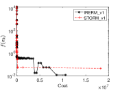
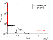
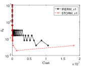
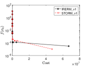
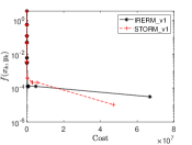
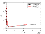
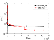
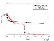
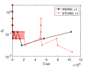
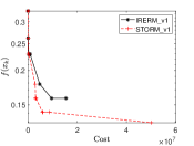
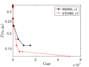
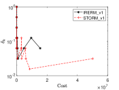
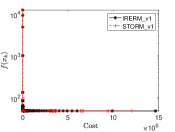
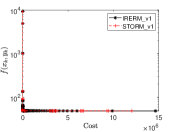
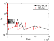
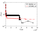
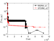
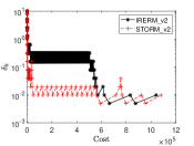
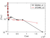
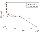
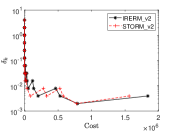
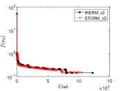
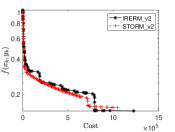
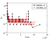
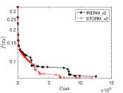
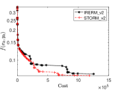
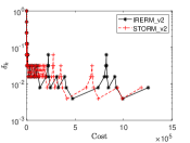
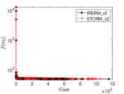
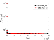
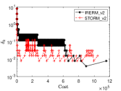
In Figure 1, we report the results obtained in the best run of irerm_v1 and storm_v1 for each problem p1–p5, namely the results corresponding to the runs where the smallest value of the exact function $f$ was achieved at termination. For each problem, we display the value of the exact function $f$ versus the computational cost (Cost), the value of the noisy function $\bar{f}$ versus the computational cost (Cost), the trust-region radius $\delta_{k}$ versus the computational cost (Cost). Figure 2 shows analogous results for irerm_v2 and storm_v2. Furthermore, in Table 2 we show the lowest values of $f$ achieved at termination over the $10$ runs by algorithms irerm_v1, storm_v1, irerm_v2, storm_v2, and in Table 3 we report the average function value of $f$ reached at termination over the 10 runs by all algorithms, respectively.

Figure 1. Best runs of irerm_v1 and storm_v1 in terms of value of $f$ at termination. From left to right: computational budget vs value of true function $f$, computational budget vs value of noisy function $\bar{f}$, computational budget vs trust-region radius $\delta_{k}$. From top to bottom: Problems p1–p5.

Figure 2. Best runs of irerm_v2 and storm_v2 in terms of value of $f$ at termination. From left to right: computational budget vs value of true function $f$, computational budget vs value of noisy function $\bar{f}$, computational budget vs trust-region radius $\delta_{k}$. From top to bottom: Problems p1–p5.

Problem	irerm_v1	storm_v1	irerm_v2	storm_v2
p1	1.15e-02	4.37e-02	2.17e-04	6.89e-03
p2	3.03e-05	1.03e-05	9.69e-11	2.33e-07
p3	5.06e-01	2.18e-01	1.43e-01	1.52e-01
p4	1.59e-01	1.29e-01	7.21e-02	6.94e-02
p5	04.85e01	04.86e01	04.74e01	04.78e01

Table 2. Lowest value of $f$ reached at termination over 10 runs for irerm and storm

Problem	irerm_v1	storm_v1	irerm_v2	storm_v2
p1	5.95e-02$\pm$3.91e-02	6.81e-02$\pm$1.65e-02	8.02e-03$\pm$1.67e-02	8.79e-03$\pm$1.73e-03
p2	1.68e-04$\pm$1.13e-04	1.98e-05$\pm$8.15e-06	1.70e-06$\pm$1.18e-06	6.31e-07$\pm$2.16e-07
p3	5.88e-01$\pm$4.50e-02	3.08e-01$\pm$3.23e-02	1.77e-01$\pm$1.30e-02	1.56e-01$\pm$2.97e-03
p4	1.59e-01$\pm$6.56e-04	1.29e-01$\pm$1.01e-04	8.10e-02$\pm$4.07e-03	7.27e-02$\pm$1.77e-03
p5	04.86e01$\pm$7.14e-02	04.92e01$\pm$2.34e-01	04.78e01$\pm$3.23e-01	04.87e01$\pm$6.48e-01

Table 3. Average function value $f$ and standard deviation at termination over 10 runs for irerm and storm

Comparing the smallest value of $f$ achieved by irerm_v1 and storm_v1, we observe in Figure 1 and Table 2 that the two solvers reach comparable values of $f$. With respect to storm_v1, irerm_v1 reached the smallest value in problem p1 and comparable values in problems p2, p3, p4 and p5. A similar behaviour occurs for the value of the noisy function at termination. In most iterations, the trust-region radius selected in irerm_v1 is larger than in storm_v1; this fact can be ascribed to the acceptance rule of the iterates, which depends on the decrease of a convex combination of the values of $\bar{f}$ and $h$, instead of using only the values $\bar{f}$ as in storm_v1. We observe that larger trust-region radii generally imply looser accuracy requirements on functions and derivatives. This feature compensates the per iteration extra cost or irerm compared to the per iteration cost of storm and makes irerm competitive with storm. The average value of $f$ reached at termination and the standard deviation of the two algorithms is summarized in Table 3. The average values and the standard deviation are similar for problems p1, p3 p4, and irerm_v1 obtained the best results in problem p5.

Comparing the smallest value of $f$ achieved by irerm_v2 and storm_v2 displayed in Figure 2 and Table 2, we note that irerm_v2 reached the smallest value of $f$ in problems p1 and p2 and compares well with storm_v2 in the remaining problems; the same occurs for the noisy values $\bar{f}$. In several iterations, the trust-region radius selected in irerm_v2 is larger than in storm_v2. Table 3 shows that the average values over 10 runs are similar for irerm_v2 and storm_v2 except for problem p2, whereas the standard deviation values are the lowest in storm_v2 except for problem p5.

The obtained results confirm that solving an unconstrained noisy problem via a suitable constrained formulation and the Inexact Restoration approach is viable and compares well with storm algorithm. Interestingly, the best results over multiple runs are good even for irerm_v2, which represents an heuristic version of our algorithm where the theoretical prescriptions are ignored. We also note that the proposed algorithm tends to compute larger trust-region radii than those of storm, which leads in some cases to smaller values of $f$ at termination of the best runs.

6. Conclusions and future work

We proposed a trust-region algorithm with first-order random models suitable for the minimization of unconstrained noisy functions. The proposed algorithm, named irerm, is based on a constrained reformulation of the minimization problem typical of the Inexact Restoration approach [1, 9, 11, 18], where the constraint $h(y)=0$ represents the ideal case in which the function and gradient estimates are computed exactly. At each iteration, irerm first enforces the sufficient accuracy in probability of the function and gradient estimates, and then employs an acceptance test involving both the noisy function and the infeasibility measure $h$. Inspired by the theoretical analysis in [7, 16], we proved an iteration complexity result for irerm, which bounds the expected number of iterations needed to achieve an approximate first-order optimality point. The numerical experiments on least-squares problems from [21] show that irerm tends to compute larger trust-region radii than other previously proposed trust-region algorithms with random models [16] and compares well with them. As future work, we plan to investigate whether it is possible to weaken the theoretical probabilistic requirements on the accuracy of function and gradient estimates, as well as design a generalized version of irerm with second-order random models.

7. Appendix

This appendix is devoted to the proof of Theorem 4.12.

Proof.

The proof follows closely [16, Theorem 4.11]. Given $\psi_{k}$ in (4.12), the successive difference $\psi_{k+1}-\psi_{k}$ can be written as

$$\psi_{k+1}-\psi_{k} =v(\theta_{k+1}f(x_{k+1})+(1-\theta_{k+1})h(y_{k+1}))$$

$$-v(\theta_{k}{f(x_{k})}+(1-\theta_{k})h(y_{k}))+v(\theta_{k+1}-\theta_{k})\Sigma+(1-v)(\delta_{k+1}^{2}-\delta_{k}^{2})$$

$$=v(\theta_{k+1}{f(x_{k+1})}+(1-\theta_{k+1})h(y_{k+1}))\pm v\theta_{k+1}{f(x_{k})}\pm v(1-\theta_{k+1})h(y_{k})$$

$$-v(\theta_{k}{f(x_{k})}+(1-\theta_{k})h(y_{k}))+v(\theta_{k+1}-\theta_{k})\Sigma+(1-v)(\delta_{k+1}^{2}-\delta_{k}^{2})$$

$$=v\left(\theta_{k+1}({f(x_{k+1})}-{f(x_{k})})+(1-\theta_{k+1})(h(y_{k+1})-h(y_{k}))\right)$$

$$+v(\theta_{k+1}-\theta_{k})({f(x_{k})}-h(y_{k})+\Sigma)+(1-v)(\delta_{k+1}^{2}-\delta_{k}^{2})$$

$$\leq v\left(\theta_{k+1}({f(x_{k+1})}-{f(x_{k})})+(1-\theta_{k+1})(h(y_{k+1})-h(y_{k}))\right)$$

(7.1) $$+(1-v)(\delta_{k+1}^{2}-\delta_{k}^{2}),$$

where the last inequality follows from (4.13) and the monotonicity of $\{\theta_{k}\}$ (see Lemma 4.3(i)). If $k$ is unsuccessful, then $x_{k+1}=x_{k}$, $y_{k+1}=y_{k}$, and $\delta_{k+1}=\delta_{k}/\gamma$ and (7) reads

(7.2) $$\psi_{k+1}-\psi_{k}\leq(1-v)\left(\frac{1-\gamma^{2}}{\gamma^{2}}\right)\delta_{k}^{2}<0.$$

To proceed, we distinguish the case $\|\nabla f(x_{k})\|\geq\zeta\delta_{k}$ from the case $\|\nabla f(x_{k})\|<\zeta\delta_{k}$.

(i) Case $\|\nabla f(x_{k})\|\geq\zeta\delta_{k}$. We analyse separately the case of true and false iteration $k$. If the iteration $k$ is true, we can combine (4.6) with $\|\nabla f(x_{k})\|\geq\zeta\delta_{k}$ to obtain

(7.3) $$\|g_{k}\|\geq\|\nabla f(x_{k})\|-\kappa\delta_{k}\geq(\zeta-\kappa)\delta_{k}\geq\max\left\{\eta_{2},\frac{\theta_{0}(3\kappa+L)}{\underline{\theta}(1-\eta_{1})}\right\}\delta_{k},$$

where in the last inequality we have applied condition (4.21). Since $k$ is true, $\kappa$ satisfies condition (4.20), $r\leq 1-\underline{\theta}(1+2\kappa)$ by assumption, and inequality (7.3) holds, Lemma 4.7 implies that $k$ is successful. Therefore, (3.3) and inequality (7) yield

$$\psi_{k+1}-\psi_{k} \leq v(\theta_{k+1}^{t}(f(x_{k}+p_{k})-f(x_{k}))+(1-\theta_{k+1}^{t})(h({y}^{t}_{k+1})-h(y_{k})))$$

$$+(1-v)(\gamma^{2}-1)\delta_{k}^{2}.$$

By summing and subtracting the quantities $\bar{f}(x_{k},\widetilde{y}_{k+1})$ and $\bar{f}(x_{k}+p_{k},y_{k+1}^{t})$ in the above inequality, we get

$$\psi_{k+1}-\psi_{k} \leq v(\theta_{k+1}^{t}(\bar{f}(x_{k}+p_{k},{y}^{t}_{k+1})-\bar{f}(x_{k},\widetilde{y}_{k+1}))+(1-\theta_{k+1}^{t})(h({y}^{t}_{k+1})-h(y_{k})))$$

$$\ \ +(1-v)(\gamma^{2}-1)\delta_{k}^{2}+v\theta_{k+1}^{t}(f(x_{k}+p_{k})-\bar{f}(x_{k}+p_{k},{y}^{t}_{k+1})$$

$$\ \ +\bar{f}(x_{k},\widetilde{y}_{k+1})-f(x_{k}))$$

$$\leq v(\theta_{k+1}^{t}(\bar{f}(x_{k}+p_{k},{y}^{t}_{k+1})-\bar{f}(x_{k},\widetilde{y}_{k+1}))+(1-\theta_{k+1}^{t})(h({y}^{t}_{k+1})-h(y_{k})))$$

$$\ \ +(1-v)(\gamma^{2}-1)\delta_{k}^{2}+v\theta_{k+1}^{t}(|f(x_{k}+p_{k})-\bar{f}(x_{k}+p_{k},{y}^{t}_{k+1})|$$

$$\ \ +|\bar{f}(x_{k},\widetilde{y}_{k+1})-f(x_{k})|).$$

By the definition of $\operatorname{Ared}_{k}$ in (3.7), the fact that $\theta_{k+1}^{t}\leq\theta_{k}\leq\theta_{0}$ (Lemma 4.3(i)), and (4.4)-(4.5) we get

(7.4) $$\psi_{k+1}-\psi_{k}\leq-v\operatorname{Ared}_{k}(x_{k}+p_{k},\theta_{k+1})+(1-v)(\gamma^{2}-1)\delta_{k}^{2}+2v\theta_{0}\kappa\delta_{k}^{2}.$$

Since we know that (4.10) holds for successful iterations, from the previous inequality we easily get

(7.5) $$\psi_{k+1}-\psi_{k}\leq-v\eta_{1}\underline{\theta}\delta_{k}\|g_{k}\|+(1-v)(\gamma^{2}-1)\delta_{k}^{2}+2v\theta_{0}\kappa\delta_{k}^{2}.$$

We exploit once again the fact that $k$ is true and $\|\nabla f(x_{k})\|\geq\zeta\delta_{k}$, and observe that

$$\|g_{k}\|\geq\|\nabla f(x_{k})\|-\kappa\delta_{k}\geq\left(1-\frac{\kappa}{\zeta}\right)\|\nabla f(x_{k})\|,$$

and (7.5) yields

$$\psi_{k+1}-\psi_{k} \leq-v\eta_{1}\underline{\theta}\left(1-\frac{\kappa}{\zeta}\right)\|\nabla f(x_{k})\|\delta_{k}+(1-v)(\gamma^{2}-1)\delta_{k}^{2}+\frac{2v\theta_{0}\kappa\delta_{k}\|\nabla f(x_{k})\|}{\zeta}$$

(7.6) $$=v\left(\frac{2\theta_{0}\kappa}{\zeta}-\eta_{1}\underline{\theta}\left(1-\frac{\kappa}{\zeta}\right)\right)\|\nabla f(x_{k})\|\delta_{k}+(1-v)(\gamma^{2}-1)\delta_{k}^{2}.$$

Note that $\frac{2\theta_{0}\kappa}{\zeta}-\eta_{1}\underline{\theta}\left(1-\frac{\kappa}{\zeta}\right)<0$ due to (4.21) and that by the definition of $C_{1}$ in (4.22), it follows

(7.7) $$\psi_{k+1}-\psi_{k}\leq-vC_{1}\delta_{k}\|\nabla f(x_{k})\|+(1-v)(\gamma^{2}-1)\delta_{k}^{2}.$$

If the iteration $k$ is false, $k$ can be either a successful or an unsuccessful iteration. If $k$ is successful, then $x_{k+1}=x_{k}+p_{k}$, and applying the Descent Lemma for functions with Lipschitz continuous gradient to $f$ leads to the following chain of inequalities

$$f(x_{k+1})-f(x_{k}) \leq\nabla f(x_{k})^{T}p_{k}+L\|p_{k}\|^{2}$$

(7.8) $$\leq\|\nabla f(x_{k})\|\delta_{k}+L\delta_{k}^{2}$$

(7.9) $$\leq\left(1+\frac{L}{\zeta}\right)\|\nabla f(x_{k})\|\delta_{k},$$

where the last inequality follows from $\|\nabla f(x_{k})\|\geq\zeta\delta_{k}$. Furthermore, we have

(7.10) $$h(y_{k+1})-h(y_{k})=h(y_{k+1}^{t})-h(y_{k})\leq(r-1)h(y_{k})\leq 0,$$

due to (3.1). Recalling the definition of $C_{2}$ in (4.22), and plugging (7.9)-(7.10) inside (7) yields

(7.11) $$\psi_{k+1}-\psi_{k}\leq v\theta_{0}C_{2}\|\nabla f(x_{k})\|\delta_{k}+(1-v)(\gamma^{2}-1)\delta_{k}^{2}.$$

If $k$ is unsuccessful, then (7.2) holds. Since the right-hand side of (7.11) is non-negative, we conclude that inequality (7.11) holds either if $k$ is successful or unsuccessful.

We are now ready to consider the expected value of $\Psi_{k+1}-\Psi_{k}$ conditioned to the past and the event $\{\|\nabla f(X_{k})\|\geq\zeta\Delta_{k}\}$. By recalling Lemma 4.10 and combining (7.7) and (7.11), we obtain

$$\mathbb{E}_{k-1}[\Psi_{k+1}-\Psi_{k}\,|\,\|\nabla f(X_{k})\|\zeta\Delta_{k}]$$

$$\quad\qquad\leq\pi(-vC_{1}\Delta_{k}\|\nabla f(X_{k})\|+(1-v)(\gamma^{2}-1)\Delta_{k}^{2})+$$

$$\quad\qquad(1-\pi)(v\theta_{0}C_{2}\|\nabla f(X_{k})\|\Delta_{k}+(1-v)(\gamma^{2}-1)\Delta_{k}^{2})$$

(7.12) $$\quad\qquad=v\|\nabla f(X_{k})\|\Delta_{k}(-C_{1}\pi+(1-\pi)\theta_{0}C_{2})+(1-v)(\gamma^{2}-1)\Delta_{k}^{2}.$$

The choice of $v$ and $\pi$ in (4.23) and (4.24) implies $\displaystyle C_{1}\pi-(1-\pi)\theta_{0}C_{2}\geq\frac{C_{1}}{2}$ and $\displaystyle\frac{C_{1}}{2}\geq\frac{2\gamma^{2}(1-v)}{v\zeta}$ and consequently

(7.13) $$C_{1}\pi-(1-\pi)\theta_{0}C_{2}\geq\frac{2(\gamma^{2}-1)(1-v)}{v\zeta}.$$

Thus (7.12) leads to

$$\mathbb{E}_{k-1}[\Psi_{k+1}-\Psi_{k}\,|\,\|\nabla f(X_{k})\|\geq\zeta\Delta_{k}] \leq-\frac{2(1-v)(\gamma^{2}-1)}{\zeta}\|\nabla f(X_{k})\|\Delta_{k}+$$

$$\qquad(1-v)(\gamma^{2}-1)\Delta_{k}^{2}$$

$$\leq-2(1-v)(\gamma^{2}-1)\Delta_{k}^{2}+(1-v)(\gamma^{2}-1)\Delta_{k}^{2}$$

$$=-(1-v)(\gamma^{2}-1)\Delta_{k}^{2},$$

where the third inequality is again due to $\|\nabla f(X_{k})\|\geq\zeta\Delta_{k}$. Thus,

(7.14) $$\mathbb{E}_{k-1}[\Psi_{k+1}-\Psi_{k}\,|\,\|\nabla f(X_{k})\|\geq\zeta\Delta_{k}]\leq-(1-v)(\gamma^{2}-1)\Delta_{k}^{2}.$$

(ii) Case $\|\nabla f(x_{k})\|<\zeta\delta_{k}$. Again, we analyse true and false iterations separately. If the iteration $k$ is true and successful, then, reasoning as in Case (i), (7.4) still holds. Thus, (7.4) and (4.10) yield

$$\psi_{k+1}-\psi_{k} \leq-v\eta_{1}\eta_{2}\underline{\theta}\delta_{k}^{2}+(1-v)(\gamma^{2}-1)\delta_{k}^{2}+2v\theta_{0}\kappa\delta_{k}^{2}$$

$$=v(2\theta_{0}\kappa-\eta_{1}\eta_{2}\underline{\theta})\delta_{k}^{2}+(1-v)(\gamma^{2}-1)\delta_{k}^{2}.$$

By (4.20), $2\theta_{0}\kappa-\eta_{1}\eta_{2}\underline{\theta}<0$ and recalling the definition of $C_{3}$ in (4.22), we get

(7.15) $$\psi_{k+1}-\psi_{k}\leq-vC_{3}\delta_{k}^{2}+(1-v)(\gamma^{2}-1)\delta_{k}^{2}=(-vC_{3}+(1-v)(\gamma^{2}-1))\delta_{k}^{2}.$$

The form of $v$ in (4.23) gives $vC_{3}\geq 2\gamma^{2}(1-v)$ and consequently $vC_{3}\geq 2(\gamma^{2}-1)(1-v)$, then (7.15) leads to

$$\psi_{k+1}-\psi_{k}\leq-(1-v)(\gamma^{2}-1)\delta_{k}^{2}.$$

If $k$ is unsuccessful, then the sufficient decrease of $\psi_{k+1}-\psi_{k}$ is guaranteed by (7.2). Since $(\gamma^{2}-1)/\gamma^{2}<\gamma^{2}-1$, we conclude that (7.2) holds for both successful and unsuccessful iterations.

If iteration $k$ is false and successful, then $x_{k+1}=x_{k}+p_{k}$, (7.8) gives

(7.16) $$f(x_{k+1})-f(x_{k}) \leq\left(\zeta+L\right)\delta_{k}^{2},$$

where the last inequality follows from $\|\nabla f(x_{k})\|<\zeta\delta_{k}$. Therefore, (7), (7.10) and (7.16) yield to

(7.17) $$\psi_{k+1}-\psi_{k}\leq(v\theta_{0}C_{4}+(1-v)(\gamma^{2}-1))\delta_{k}^{2},$$

with $C_{4}$ given in (4.22).

If $k$ is unsuccessful, then (7.2) holds, and thus $\psi_{k+1}-\psi_{k}<0$. Since the right-hand side of (7.17) is non-negative, we conclude that inequality (7.17) holds either if $k$ is successful or unsuccessful.

By taking the expected value of $\Psi_{k+1}-\Psi_{k}$ conditioned to the past and the event $\|\nabla f(X_{k})\|<\zeta\Delta_{k}$, and combining (7.2) with (7.17), we obtain

$$\mathbb{E}_{k-1}[\Psi_{k+1}-\Psi_{k}\,|\,\|\nabla f(X_{k})\|<\zeta\Delta_{k}]$$

$$\qquad\leq\pi(1-v)\left(\frac{1-\gamma^{2}}{\gamma^{2}}\right)\Delta_{k}^{2}+(1-\pi)(v\theta_{0}C_{4}+(1-v)(\gamma^{2}-1))\Delta_{k}^{2}$$

$$\qquad=(\pi\pm 1)(1-v)\left(\frac{1-\gamma^{2}}{\gamma^{2}}\right)\Delta_{k}^{2}+(1-\pi)(v\theta_{0}C_{4}+(1-v)(\gamma^{2}-1))\Delta_{k}^{2}$$

$$\qquad=(1-v)\left(\frac{1-\gamma^{2}}{\gamma^{2}}\right)\Delta_{k}^{2}+(1-\pi)\left(v\theta_{0}C_{4}+(1-v)\left(\frac{\gamma^{4}-1}{\gamma^{2}}\right)\right)\Delta_{k}^{2}.$$

The choice of $\pi$ in (4.24) gives $(1-\pi)\left(v\theta_{0}C_{4}+(1-v)\left(\frac{\gamma^{4}-1}{\gamma^{2}}\right)\right)\leq\frac{1}{2}(1-v)\left(\frac{\gamma^{2}-1}{\gamma^{2}}\right)$,

(7.18) $$\mathbb{E}_{k-1}[\Psi_{k+1}-\Psi_{k}\,|\,\|\nabla f(X_{k})\|<\zeta\Delta_{k}]\leq-\frac{1}{2}(1-v)\left(\frac{\gamma^{2}-1}{\gamma^{2}}\right)\Delta_{k}^{2}.$$

Finally, by combining (7.14) and (7.18) and observing that $(\gamma^{2}-1)/(2\gamma^{2})<\gamma^{2}-1$, we obtain

(7.19) $$\mathbb{E}_{k-1}[\Psi_{k+1}-\Psi_{k}]\leq-\frac{1}{2}(1-v)\left(\frac{\gamma^{2}-1}{\gamma^{2}}\right)\Delta_{k}^{2},$$

and we conclude that (4.25) holds with $\sigma=\frac{1}{2}(1-v)(\gamma^{2}-1)/\gamma^{2}$.

In order to prove (4.26), summing (4.25) over $k=0,\ldots,K$, one gets

$$\sum_{k=0}^{K}\sigma\Delta_{k}^{2}\leq\sum_{k=0}^{K}\mathbb{E}_{k-1}[\Psi_{k}-\Psi_{k+1}].$$

By taking the total expected value and recalling the definition of conditional expected value, we obtain

$$\mathbb{E}\left[\sum_{k=0}^{K}\sigma\Delta_{k}^{2}\right] =\sum_{k=0}^{K}\mathbb{E}\left[\mathbb{E}_{k-1}[\Psi_{k}-\Psi_{k+1}]\right]$$

$$=\mathbb{E}\left[\sum_{k=0}^{K}(\Psi_{k}-\Psi_{k+1})\right]$$

$$\leq\mathbb{E}[\Psi_{0}-\Psi_{low}],$$

where the last inequality is due to the fact that $\{\Psi_{k}\}$ is bounded from below by a constant $\Psi_{low}$ for all $k\geq 0$, thanks to Assumption 2.1(i) and (iii). By taking the limit for $K\rightarrow\infty$ and applying the monotone convergence theorem on the left-hand side of the inequality, we get $\mathbb{E}\left[\sum_{k=0}^{\infty}\Delta_{k}^{2}\right]<\infty$ from which (4.26) immediately follows. ∎

References

- [1] M. B. Arouxét, N. E. Echebest, E. A. Pilotta, Inexact Restoration method for nonlinear optimization without derivatives, Journal of Computational and Applied Mathematics, 290(15), 26–43, 2015.
- [2] A. S Bandeira, K. Scheinberg, L. N. Vicente, Convergence of trust-region methods based on probabilistic models, SIAM Journal on Optimization, 24(3), 1238–1264, 2014.
- [3] S. Bellavia, G. Gurioli, B. Morini, Ph. L. Toint, Trust-region algorithms: probabilistic complexity and intrinsic noise with applications to subsampling techniques, EURO Journal on Computational Optimization, 10, 100043, 2022.
- [4] S. Bellavia, N. Krejić, B. Morini, S. Rebegoldi, A stochastic first-order trust-region method with inexact restoration for finite-sum minimization, Computational Optimization and Applications, 84, 53–84, 2023.
- [5] S. Bellavia, N. Krejić, B. Morini, Inexact restoration with subsampled trust-region methods for finite-sum minimization, Computational Optimization and Applications 76, 701–736, 2020.
- [6] S. Bellavia, B. Morini, S. Rebegoldi, On the Convergence Properties of a Stochastic Trust-Region Method with Inexact Restoration, Axioms, 12(1), 38, 2023.
- [7] J. Blanchet, C. Cartis, M. Menickelly, K. Scheinberg, Convergence Rate Analysis of a Stochastic Trust Region Method via Submartingales, INFORMS Journal on Optimization, 1, 92–119, 2019.
- [8] R. Bollapragada, R. Byrd, J. Nocedal, Adaptive sampling strategies for stochastic optimization, SIAM Journal on Optimization 28(4), 3312–3343, 2018.
- [9] L. F. Bueno, J. M. Martínez, On the Complexity of an Inexact Restoration Method for Constrained Optimization, SIAM Journal on Optimization 30, 80–101, 2020.
- [10] L. F. Bueno, F. Larreal, J. M. Martínez, Inexact restoration for minimization with inexact evaluation both of the objective function and the constraints, Mathematics of Computation, 93, 293–326, 2024.
- [11] L. F. Bueno, G. Haeser, J. M. Martínez, A flexible inexact restoration method for constrained optimization, Journal of Optimization Theory and Applications, 165, 188–208, 2015.
- [12] E. G. Birgin, N. Krejić, J. M. Martínez, On the employment of Inexact Restoration for the minimization of functions whose evaluation is subject to programming errors, Mathematics of Computation 87, 311, 1307–1326, 2018.
- [13] E. G. Birgin, N. Krejić, J. M. Martínez, Iteration and evaluation complexity on the minimization of functions whose computation is intrinsically inexact, Mathematics of Computation 89, 253–278, 2020.
- [14] E. G. Birgin, N. Krejić, J. M. Martínez, Iteration and evaluation complexity on the minimization of functions whose computation is intrinsically inexact, Mathematics of Computation 89, 253–278, 2022.
- [15] L. Bottou, F. C. Curtis, J. Nocedal, Optimization methods for large-scale machine learning, SIAM Review, 60, 2, 223–311, 2018.
- [16] R. Chen, M. Menickelly, K. Scheinberg, Stochastic optimization using a trust-region method and random models, Mathematical Programming 169(2), 447–487, 2018.
- [17] F. E. Curtis, K. Scheinberg, Adaptive Stochastic Optimization: A Framework for Analyzing Stochastic Optimization Algorithms, IEEE Signal Processing Magazine, 37(5), 32–42, 2020.
- [18] A. Fischer, A. Friedlander, A new line search inexact restoration approach for nonlinear programming, Computational Optimization and Applications, 46, 336–346, 2010.
- [19] N. Krejić, J. M. Martínez, Inexact Restoration approach for minimization with inexact evaluation of the objective function, Mathematics of Computation, 85, 1775–1791, 2016.
- [20] J. Larson, S.C. Billups, Stochastic derivative-free optimization using a trust region framework, Computational Optimization and Applications, 64, 619–645, 2016.
- [21] L. Luks̆an, C. Matonoha, J Vlc̆ek, Problems for Nonlinear Least Squares and Nonlinear Equations, Technical report No. 1259, Institute of Computer Science Academy of Sciences of the Czech Republic, 2018.
- [22] J. M. Martínez, E. A. Pilotta, Inexact restoration algorithms for constrained optimization, Journal of Optimization Theory and Applications, 104, 135–163, 2000.
- [23] J. C. Spall, Introduction to Stochastic Search and Optimization: Estimation, Simulation, and Control, Wiley Series in Discrete Mathematics and Optimization. Wiley, London, 2005.
- [24] J. A. Tropp, An Introduction to Matrix Concentration Inequalities, Foundations & Trends in Machine Learning, Vol. 8, num. 1–2, pp. 1–230, 2015.
- [25] J. Willert, X. Chen, C T. Kelly, Newton’s method for Monte Carlo-based residuals, SIAM Journal of Numerical Analysis, 53(4), 1738–1757, 2015.