To test $R_{NLRs}~{}-~{}L_{O3}$ relation for narrow emission line regions of AGN through low redshift Type-2 AGN in SDSS

Abstract

Sizes of narrow emission line regions (NLRs) of AGN could be estimated by [O iii]  line luminosity $L_{O3}$ through the known $R_{NLRs}-L_{O3}$ empirical relations. Unfortunately, it is not convenient to test the $R_{NLRs}-L_{O3}$ empirical relations through structure properties of spatially resolved NLRs of large samples of AGN. In this manuscript, a method is proposed to test the $R_{NLRs}-L_{O3}^{\sim 0.25}$ empirical relations for AGN NLRs through SDSS Type-2 AGN having few orientation effects on NLRs sizes expected by AGN unified model, after considering sizes $R_{fib}$ of SDSS fiber covered regions. Comparing $R_{fib}$ and $R_{NLRs}$ estimated by $L_{O3}$, Type-2 AGN with $R_{fib}>R_{NLRs}$ (Sample-II) and with $R_{fib}<R_{NLRs}$ (Sample-I) should have different physical properties of NLRs. Accepted electron density gradients in AGN NLRs, statistically higher electron densities (traced by lower flux ratio $R_{S2}$ of [S ii]$\lambda 6717$Å  to [S ii]$\lambda 6731$Å) could be expected for the Type-2 AGN in the Sample-I. Then, through the collected 1062 SDSS Type-2 AGN in the Sample-I and 3658 SDSS Type-2 AGN in the Sample-II, statistically lower $R_{S2}$ for the Type-2 AGN in the Sample-I can be confirmed with confidence level higher than 5$\sigma$, even after considering necessary effects. Therefore, the results in this manuscript can provide strong clues to support that the reported $R_{NLRs}~{}\propto~{}L_{O3}^{0.25}$ empirical relation is preferred to estimate NLRs sizes of SDSS AGN through SDSS fiber spectroscopic results, and also to support the commonly expected electron density gradients in AGN NLRs.

1 Introduction

Narrow emission line regions (NLRs) at kilo-parsec (kpc) scales to central black holes (BHs) are fundamental structures of active galactic nuclei (AGN) (Netzer & Laor, 1993; Netzer et al., 2004; Stoklasova et al., 2009; Shen et al., 2011; Dopita et al., 2015; Gomez-Guijarro et al., 2017; Thomas et al., 2018; Mignoli et al., 2019; Meena et al., 2023). So large spatial distance to central BHs and extended structures, NLRs in nearby AGN with high luminous [O iii]  emissions can be well spatially resolved, leading to well determined sizes of AGN NLRs ($R_{NLRs}$, distance between NLRs to central BHs). Then, the known $R_{NLRs}-L_{O3}$ empirical relation is proposed to estimate $R_{NLRs}$ through well measured [O iii]  line luminosity $L_{O3}$,

$$\log(\frac{R_{NLRs}}{\rm pc})\propto~{}0.25\log(\frac{L_{O3}}{\rm 10^{42}erg/s})$$ (1)

. The equation above is firstly reported in Liu et al. (2013) through Gemini Integral Field Unit observations of spatially resolved [O iii] emission regions in a sample of low redshift ($z\sim 0.5$) radio quiet Type-2 quasars, and then well discussed in Hainline et al. (2013, 2014) for an upper limit for $R_{NLRs}$ in high luminous quasars. Sun et al. (2018) have reported the similar dependence of $R_{NLRs}$ on $L_{O3}^{0.22-0.33}$ through a new broad-band imaging technique to reconstruct the spatial structures of the [O iii] emission regions of 300 obscured AGN at redshifts 0.1-0.7. Husemann et al. (2022) have shown the similar dependence (but with large scatters) of $R_{NLRs}$ on $L_{O3}^{0.25-0.29}$ through wide-field optical integral-field unit spectroscopy for 41 luminous unobscured AGN with $z<0.06$ in the Close AGN Reference Survey. More recently, we Zhang (2022) have tested the $R_{NLRs}-L_{O3}^{\sim 0.25}$ empirical relation through a sample of AGN with double-peaked broad Balmer emission lines.

Meanwhile, besides the reported $R_{NLRs}-L_{O3}$ empirical relation with slope about 0.25 in Liu et al. (2013); Sun et al. (2018); Husemann et al. (2022), there are $R_{NLRs}-L_{O3}$ relations with different slopes found in the literature. Schmitt et al. (2003); Fischer et al. (2018) have reported one $R_{NLRs}-L_{O3}$ relation with slope about 0.4-0.5, through Hubble Space Telescope (HST) observations of [O iii] emission regions in samples of Seyfert 2 galaxies and/or Type-2 quasars. As discussed in Liu et al. (2013), different $R_{NLRs}-L_{O3}$ relation in Schmitt et al. (2003); Fischer et al. (2018) from the one in Liu et al. (2013) could be due to HST observations being 1-2 magnitudes shallower than the Gemini Integral Field Unit observations and long-slit spectroscopy applied in Liu et al. (2013). More recently, Chen et al. (2019) have reported $R_{NLRs}-L_{O3}^{\sim 0.42}$ through spatially resolved structures of extended narrow line regions of a large sample of nearby AGN from the Mapping Nearby Galaxies at Apache Point Observatory survey.

Furthermore, besides the discussed $R_{NLRs}-L_{O3}$ empirical relations through observations, more recent review on theoretically expected $R_{NLRs}-L_{O3}$ relations can be found in Dempsey & Zakamska (2018) through modelling AGN NLRs as a collection of clouds in pressure equilibrium with the ionizing radiation. The $R_{NLRs}-L_{O3}$ empirical relations reported in Liu et al. (2013) and in Fischer et al. (2018) can be both theoretically explained by different model parameters in Dempsey & Zakamska (2018).

Until now, only a few tens of AGN have their NLRs spatially resolved leading to well estimated $R_{NLRs}$, to test the predicted $R_{NLRs}-L_{O3}$ empirical relations through NLRs properties in a large sample of AGN should be very interesting and necessary. Unfortunately, it is not convenient to spatially resolve NLRs in samples of AGN. Therefore, in this manuscript, an indirect method is proposed to test $R_{NLRs}-L_{O3}$ empirical relations through a large sample of low redshift Type-2 AGN in SDSS, after considering natural applications of 3″  fiber diameters for SDSS spectroscopic results and properties of AGN unified model expected projected space size of NLRs in Type-2 AGN, which is the main objective of this manuscript.

The known AGN unified model has been well discussed in Antonucci (1993); Bianchi et al. (2012); Marinucci et al. (2012); Oh et al. (2015); Netzer (2015); Mateos et al. (2016); Audibert et al. (2017); Balokovic et al. (2018); Brown et al. (2019); Kuraszkiewicz et al. (2021); Zhang (2022, 2023) to well explain different observational phenomena between broad line AGN and narrow line AGN (Type-2 AGN). The commonly accepted AGN unified model indicates few orientation effects on estimated $R_{NLRs}$ in Type-2 AGN. Therefore, a large sample of low redshift Type-2 AGN collected from Sloan Digital Sky Survey (SDSS) are mainly considered in the manuscript. Moreover, considering fixed fiber diameters for SDSS spectra, fiber expected projected space sizes can be applied to test different physical properties of NLRs in Type-2 AGN, as well described in Section 2.

In this manuscript, section 2 presents our main hypotheses. Section 3 shows our main results and necessary discussions. Section 4 gives our main summary and conclusions. And in the manuscript, the cosmological parameters of $H_{0}~{}=~{}70{\rm km\cdot s}^{-1}{\rm Mpc}^{-1}$, $\Omega_{\Lambda}~{}=~{}0.7$ and $\Omega_{m}~{}=~{}0.3$ have been adopted.

2 Main Hypotheses

Due to fixed fiber diameter 3″  for SDSS spectra, sizes of [O iii]  emissions ($R_{NLRs}$, distance between NLRs and central BHs) in SDSS spectrum of a Type-2 AGN can be discussed by the following two cases. First, if [O iii]  emissions of a Type-2 AGN were totally covered by the SDSS fiber, intrinsic $R_{NLRs}$ (with few effects of orientation effects) should be smaller than $R_{fib}=1.5$″, meanwhile the measured [O iii]  line luminosity was the intrinsic value. Second, if [O iii]  emissions of a Type-2 AGN were partly covered by the SDSS fiber, intrinsic $R_{NLRs}$ should be larger than $R_{fib}=1.5$″, meanwhile, the measured [O iii]  line luminosity should be smaller than the intrinsic value.

Comparing estimated $R_{NLRs}$ by observed [O iii]  line luminosity and fiber expected $R_{fib}$, the collected SDSS Type-2 AGN can be divided into two samples, one sample (sample-I) of Type-2 AGN with $R_{NLRs}~{}>~{}R_{fib}$ and the other sample (sample-II) of Type-2 AGN with $R_{NLRs}~{}<~{}R_{fib}$. Then, considering dependence of spatially resolved electron density on distance of emission regions to central BHs as well shown and discussed in Kakkad et al. (2018); Kewley et al. (2019a), i.e. apparent electron density gradients in AGN NLRs, SDSS Type-2 AGN in the Sample-1 should have statistically higher electron densities determined through spectroscopic features than SDSS Type-2 AGN in the sample-II, due to NLRs with lower electron densities not covered by the SDSS fibers for spectra of Type-2 AGN in the sample-I. Certainly, if there were no apparent electron density gradients in AGN NLRs, i.e. constant electron density distributions in AGN NLRs, some further properties on NLRs should be further proposed in this manuscript. Therefore, it is interesting to check spectroscopic properties of SDSS Type-2 AGN in the Sample-I and in the Sample-II.

Furthermore, it is very convenient to estimate electron density in AGN NLRs, through emission line flux ratio $R_{S2}$ of [S ii]$\lambda 6716$Å  to [S ii]$\lambda 6731$Å  as well discussed in Sanders et al. (2016); Kawasaki et al. (2017); Kewley et al. (2019a, b); Flury & Moran (2020); Kazuma et al. (2021); Riffel et al. (2021); Dors et al. (2022); Zhang (2023). Therefore, once large samples of SDSS Type-2 AGN are created, properties of electron density in AGN NLRs can be easily determined, which will provide further clues not only to (or not to) support the reported $R_{NLRs}-L_{O3}$ empirical relations with different slopes in the literature but also to (or not to) support electron density gradients in AGN NLRs.

Finally, if accepted electron density gradients in AGN NLRs, considering $R_{S2}$ to trace electron densities in AGN NLRs (lower $R_{S2}$ indicating higher electron densities), we would have

$$R_{S2}(Sample-I)~{}<~{}R_{S2}(Sample-II)$$ (2)

, which is the basic point applied to test $R_{NLRs}-L_{O3}$ empirical relations in the manuscript.

3 Main Results and Necessary Discussions

3.1 Type-2 AGN in main sample

As well described in https://www.sdss.org/dr16/spectro/catalogs/, each spectroscopic object has a classification in SDSS. Simple criteria can be well applied to conveniently collect all the low redshift pipeline classified Type-2 AGN from SDSS main narrow emission line galaxies in data release 16 (DR16) (Ahumada et al., 2020), through the SDSS provided SQL (Structured Query Language) Search tool (http://skyserver.sdss.org/dr16/en/tools/search/sql.aspx) by the following query

⬇

SELECT plate, fiberid, mjd, z, G.sii_6717_flux,

G.sii_6731_flux, G.oiii_5007_flux,

G.nii_6584_flux, G.h_alpha_flux,

G.h_beta_flux, G.oiii_4363_flux,

G.oiii_4363_flux_err

FROM SpecObjall as S JOIN GalSpecLine as G

on S.specobjid = G.specobjid

WHERE

class=’galaxy’ and subclass = ’AGN’ and

z < 0.3 and zwarning = 0

and G.sii_6717_flux_err > 0 and

G.sii_6717_flux > 5*G.sii_6717_flux_err

and G.sii_6731_flux_err > 0 and

G.sii_6731_flux > 5*G.sii_6731_flux_err

and G.oiii_5007_flux_err > 0 and

G.oiii_5007_flux > 5*G.oiii_5007_flux_err

and G.nii_6584_flux_err > 0 and

G.nii_6584_flux > 5*G.nii_6584_flux_err

and G.h_alpha_flux_err > 0 and

G.h_alpha_flux > 5*G.h_alpha_flux_err

and G.h_beta_flux_err > 0 and

G.h_beta_flux > 5*G.h_beta_flux_err

The SQL query above can lead 11803 narrow emission line galaxies (pipeline classified Type-2 AGN) to be collected into our main sample.

In the query above, ’SpecObjall’ is the SDSS pipeline provided database (http://skyserver.sdss.org/dr16/en/help/docs/tabledesc.aspx) including basic properties of spectroscopic features of emission line galaxies in SDSS DR16, ’GalSpecLine’ is the database including measured line parameters of emission lines provided by the MPA-JHU group as well described in https://www.sdss.org/dr16/spectro/galaxy_mpajhu/ and in Brinchmann et al. (2004); Kauffmann et al. (2003a); Tremonti et al. (2004). In the query above, class=’galaxy’ and subclass=’AGN’ mean SDSS spectrum can be well identified with a galaxy template and the galaxy has detectable emission lines that are consistent with being a Seyfert-2 or a LINER classified by BPT diagram (Baldwin et al., 1981; Kewley et al., 2001; Kauffmann et al., 2003a; Kewley et al., 2006, 2019a; Zhang et al., 2020). In the query above, z < 0.3 and zwarning = 0 are applied to confirm [S ii] doublet covered by SDSS spectra with reliable pipeline determined redshift. In the query above, G.oiii_5007_flux_err > 0 and G.oiii_5007_flux > 5*G.oiii_5007_flux_err and G.sii_6717_flux_err > 0 and G.sii_6717_flux > 5*G.sii_6717_flux_err and G.sii_6731_flux_err > 0 and G.sii_6731_flux > 5*G.sii_6731_flux_err and G.nii_6584_flux_err > 0 and G.nii_6584_flux > 5*G.nii_6584_flux_err and G.h_alpha_flux_err > 0 and G.h_alpha_flux > 5*G.h_alpha_flux_err and G.h_beta_flux_err > 0 and G.h_beta_flux > 5*G.h_beta_flux_err are applied to confirm reliable measurements of [O iii] , [S ii], [N ii] and narrow Balmer emission line fluxes which will be applied in this manuscript, considering measured line fluxes at least 5 times larger than their uncertainties.

Before proceeding further, one point is noted. As what we have recently checked and shown in Zhang (2023), the ’GalSpecLine’ provided measured fluxes of narrow emission lines in Type-2 AGN are reliable enough, and there are no further discussions in this manuscript on effects of measurements of emission line fluxes on reliability of following statistical results.

Figure 1: BPT diagrams in contour of O3HB versus N2HA (top panel) and of O3HB versus S2HA (bottom panel) of the collected 11803 objects. Contour levels in different colors are related to number densities shown in color bar in top region of each panel. Dashed green line in each panel shows the extremely dividing line between AGN and HII galaxies reported in Kewley et al. (2006). Solid green line in top panel shows the dividing line between HII galaxies and composite galaxies reported in Kauffmann et al. (2003). Dashed red line in bottom panel shows the dividing line between AGN and LINERs reported in Kewley et al. (2006).

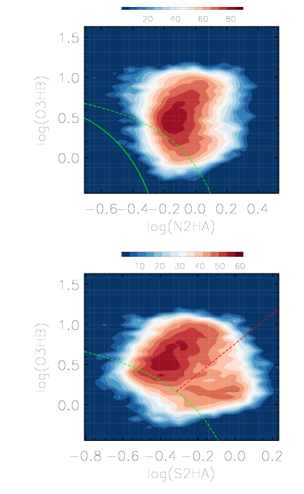
Then, Fig. 1 shows BPT diagrams of flux ratio of [O iii]  to narrow H$\beta$ (O3HB) versus flux ratio of [N ii] to narrow H$\alpha$ (N2HA) and of O3HB versus flux ratio of [S ii] to narrow H$\alpha$ (S2HA) of the collected 11803 Type-2 AGN in our main sample. Due to SDSS pipeline provided AGN classifications (objects lying above solid green line in top panel of Fig. 1) only through flux ratios of O3HB and N2HA, part of collected objects in the main sample are lying into HII regions (below dashed green line in bottom panel of Fig. 1) in the BPT diagram of S2HA versus O3HB. Furthermore, as different physical mechanisms discussed in the literature (Heckman, 1980; Dopita & Sutherland, 1996; Filippenko & Terlevich, 1992; Eracleous et al., 2010; Cid Fernandes et al., 2011; Marquez et al., 2017), there are no confirmed conclusions on LINERs as genuine AGN. Therefore, in the manuscript, LINERs are not considered. The dividing line (dashed red line in bottom panel of Fig. 1) in Kewley et al. (2006) is applied to identify LINERs in the BPT diagram of S2HA versus O3HB. In order to ignore probable effects from starforming and LINERs, we only consider the 7355 objects classified as AGN both in the BPT diagram of N2HA versus O3HB and in the BPT diagram of S2HA versus O3HB, i.e., the objects lying not only above the dashed green line in top panel of Fig. 1 but also above the dashed red line in bottom panel of Fig. 1.

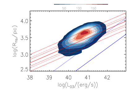
Then, Fig. 2 shows dependence of $R_{fib}$ (in units of pc, calculated by fiber radius and corresponding redshift) on observed [O iii]  line luminosity of the collected 7355 Type-2 AGN, and also the $R_{NLRs}-L_{O3}^{0.25}$ empirical relation in Liu et al. (2013). Interestingly, part of Type-2 AGN have $R_{fib}$ clearly larger than $R_{NLRs}-L_{O3}$ empirical relation expected values, but part of Type-2 AGN have $R_{fib}$ apparently smaller than $R_{NLRs}-L_{O3}$ empirical relation expected values. As discussed in Section 2, Type-2 AGN above and below the $R_{NLRs}-L_{O3}$ empirical relation in Fig. 2 should have expected different electron densities in their NLRs. Further discussions on $R_{NLRs}-L_{O3}^{0.4-0.5}$ will be given in Section 3.

Figure 2: Correlation in contour between SDSS fiber radii $R_{fib}$ in units of pc and observed $L_{O3}$ of the 7355 Type-2 AGN. Contour levels in different colors are related to number densities shown in color bar in top region. Solid red line, dashed red lines, dotted red lines and dot-dashed red lines show the $R_{NLRs}-L_{O3}$ relation reported in Liu et al. (2013) and corresponding 2RMS, 3RMS and 5RMS scatters. Solid blue line shows the reported $R_{NLRs}-L_{O3}$ relation in Fischer et al. (2018). Dotted blue line shows the reported $R_{NLRs}-L_{O3}$ relation in Chen et al. (2019).

Figure 3: Distributions of $\log(R_{S2})$ of the Type-2 AGN in the Sample-II (histogram filled by blue lines) and in the Sample-I (histogram filled by red lines). Thick dashed line shows Gaussian-like descriptions to the histogram in the same color. Vertical dark green line marks the position of $R_{S2}=1.5$. Vertical thick lines in blue and in red in top region mark positions of median values of $\log(R_{S2})$ of the Type-2 AGN with $R_{S2}<1.5$ in the Sample-II and in the Sample-I.

Figure 4: On the dependence of $\log(R_{S2})$ on redshift for the Type-2 AGN in the Sample-II (contour filled by bluish colors) and in the Sample-I (contour levels labelled and shown in reddish colors). Contour levels in different colors are related to number densities shown in the color bars in the top region. Horizontal dark green line marks the position of $R_{S2}=1.5$.

Figure 5: Distributions of redshift (in top panel) and $\log(R_{S2})$ (in bottom panel) of the Type-2 AGN in the subsample-II (histogram filled by blue lines) and in the subsample-I (histogram filled by red lines). In bottom panel, thick dashed line shows Gaussian-like descriptions to the histogram in the same color, vertical dark green line marks the position of $R_{S2}=1.5$, vertical thick lines in blue and in red in top region mark positions of the median values of $\log(R_{S2})$ of the Type-2 AGN with $R_{S2}<1.5$ in the subsample-II and in the subsample-I.

3.2 Main Results and Discussions

Based on Fig. 2 and considering the RMS scatter about 0.05 of the $R_{NLRs}-L_{O3}$ empirical relation in Liu et al. (2013), two samples of Type-2 AGN are created, one sample (Sample-II) of Type-2 AGN includes the 3658 Type-2 AGN lying above the $R_{NLRs}-L_{O3}$ empirical relation plus 2RMS scatter and the other sample (Sample-I) of Type-2 AGN includes the 1062 Type-2 AGN lying below the $R_{NLRs}-L_{O3}$ empirical relation minus 2RMS scatter. Here, applications of $R_{NLRs}-L_{O3}$ relation plus/minus 2RMS scatter can not only lead as many Type-2 AGN as possible to be collected into following Sample-I and Sample-II, but also lead to few effects of scatters of the $R_{NLRs}-L_{O3}$ empirical relation on our following statistical results. And applications of $R_{NLRs}-L_{O3}$ relation plus/minus 3RMS scatters and 5RMS scatters will be discussed before the end of the subsection in this manuscript.

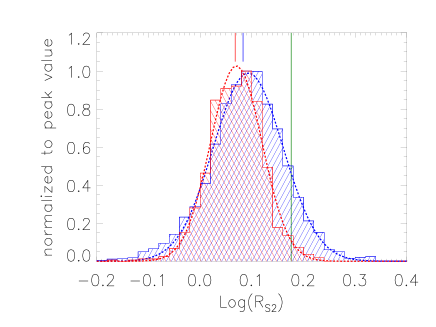
Then, Fig. 3 shows $R_{S2}$ distributions of the Type-2 AGN in the Sample-I and in the Sample-II. Meanwhile, as noted in Kawasaki et al. (2017); Kewley et al. (2019b) that when $R_{S2}$ is applied to trace electron density, $R_{S2}$ should be effectively limited to the range from 0.4 to 1.5, i.e., $-0.4~{}<~{}\log(R_{S2})~{}<~{}0.18$. Therefore, objects with $\log(R_{S2})~{}>~{}0.18$ should be not considered to trace electron density. The median values of $\log(R_{S2})$ (with $R_{S2}<1.5$) are about $(8.31\pm 0.13)\times 10^{-2}$ and $(6.79\pm 0.15)\times 10^{-2}$ for the Type-2 AGN in the Sample-II and in the Sample-I, respectively. Uncertainties of the median values are estimated by the bootstrap method within 1000 loops, as what we have recently done in Zhang (2023). For each loop, about half of the data points of $\log(R_{S2})$ ($R_{S2}<1.5$) of the Type-2 AGN in the Sample-I or in the Sample-II are randomly collected to create a new sample, leading to a re-measured median value. After 1000 loops, based on distribution of the 1000 re-measured median values, half width at half maximum of the distribution is accepted as the uncertainty of the median value. It is clear that there are quite different median values of $\log(R_{S2})$ (with $R_{S2}<1.5$) for the Type-2 AGN in the Sample-II and in the Sample-I. Meanwhile, through the Wilcoxon Rank-Sum Test, the Type-2 AGN in the subsample-II and in the subsample-I have the same median values of $\log(R_{S2})$ (with $R_{S2}<1.5$) with significance level smaller than $10^{-17}$. Moreover, the lower median value of $\log(R_{S2})$ (with $R_{S2}<1.5$) in the Type-2 AGN in the Sample-I is consistent with what we can expected (as discussed in Section 2) for Type-2 AGN in Sample-I having their NLRs partly covered by SDSS fibers.

Before proceeding further, the following seventh points should be discussed to confirm different $\log(R_{S2})$ (with $R_{S2}<1.5$) of the Type-2 AGN in the Sample-I and in the Sample-II.

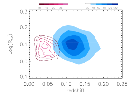
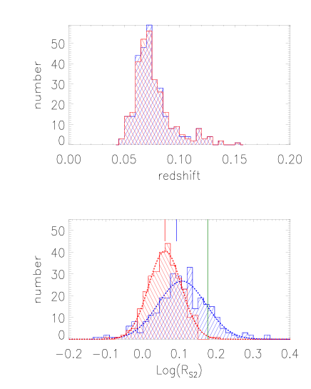
First, there are apparently different redshift distributions of the Type-2 AGN in the Sample-II and in the Sample-I, as shown in Fig. 4 with mean redshift about 0.13 and 0.05. Therefore, it is necessary to discuss effects of different redshift distributions on comparing $\log(R_{S2})$ (with $R_{S2}<1.5$) shown in Fig. 3 of the Type-2 AGN in the Sample-II and in the Sample-I. Then, the following two methods are applied. On the one hand, the dependence of $\log(R_{S2})$ on redshift shown in Fig. 4 is firstly checked. The Spearman Rank correlation coefficients are about -0.12 ($P_{null}\sim 8\times 10^{-14}$) and -0.13 ($P_{null}\sim 1\times 10^{-5}$) for the Type-2 AGN in the Sample-II and in the Sample-I, respectively. Not different dependence of $\log(R_{S2})$ on redshift indicates few effects of different redshift distributions on the statistically different $\log(R_{S2})$ for the Type-2 AGN in the Sample-I and in the Sample-II. On the other hand, among the Type-2 AGN in the Sample-II and in the Sample-I, two subsamples, one subsample (subsample-II) including 301 Type-2 AGN from the Sample-II and the other subsample (subsample-I) including 301 Type-2 AGN from the Sample-I, can be simply created to have the same redshift distributions with significance levels higher than 99.91% through the two-sided Kolmogorov-Smirnov statistic technique, similar as what we have recently done in Zhang (2023) through finding the minimum parameter distance. The same redshift distributions of Type-2 AGN in the subsamples are shown in top panel of Fig. 5. Meanwhile, bottom panel of Fig. 5 shows $\log(R_{S2})$ distributions of the Type-2 AGN in the two subsamples. The median values and the corresponding bootstrap method determined uncertainties of $\log(R_{S2})$ (with $R_{S2}<1.5$) are about $(9.13\pm 0.24)\times 10^{-2}$ and $(6.01\pm 0.21)\times 10^{-2}$ for the Type-2 AGN in the subsample-II and in the subsample-I, respectively. And through the Wilcoxon Rank-Sum Test, the Type-2 AGN in the subsample-II and in the subsample-I have the same median values of $\log(R_{S2})$ (with $R_{S2}<1.5$) with significance level smaller than $10^{-17}$. Therefore, there are no dependence of $\log(R_{S2})$ on redshift, indicating few effects of different redshift distributions on different $\log(R_{S2})$ for the Type-2 AGN in the Sample-II and in the Sample-I.

Second, due to the discussed results above mainly based on collected Type-2 AGN in the Sample-I and the Sample-II through considering 2RMS scatters of the $R_{NLRs}-L_{O3}$ empirical relation in Liu et al. (2013), it is necessary to check whether $k\times$RMS ($k$ larger than 2) scatters applied can lead to different results. Here, 3RMS (5RMS) scatters are applied to build a new Sample-I including 736 (363) Type-2 AGN and a new Sample-II including 2746 (1135) Type-2 AGN. Considering 3RMS (5RMS) scatters can lead median values and the corresponding bootstrap method determined uncertainties of $\log(R_{S2})$ (with $R_{S2}<1.5$) to be about $(7.88\pm 0.17)\times 10^{-2}$ and $(6.32\pm 0.21)\times 10^{-2}$ ($(7.08\pm 0.24)\times 10^{-2}$ and $(5.93\pm 0.23)\times 10^{-2}$) for the Type-2 AGN in the new Sample-II and in the new Sample-I, respectively. And considering 3RMS (5RMS) scatters, the Wilcoxon Rank-Sum Test can be applied to confirm significantly different median values of $\log(R_{S2})$ with significance level about $10^{-17}$ ($10^{-8}$) (confidence level higher than 5$\sigma$) of the Type-2 AGN in the new Sample-I and in the new Sample-II. Therefore, different criteria on RMS scatters have few effects on the different median $\log(R_{S2})$ of the Type-2 AGN in the Sample-I and in the Sample-II.

Figure 6: Dependence of $R_{S2}$ on distance $Dis$ of objects to the $R_{NLRs}-L$ empirical relation in Liu et al. (2013). Contour in left region shows the results for the 1062 Type-2 AGN in the Sample-I, and contour in right region shows the results for the 3658 Type-2 AGN in the Sample-II. Solid red line and dashed red lines show the linearly dependence and the corresponding 1RMS scatter of $\log(R_{S2})$ on $Dis$ for the Type-2 AGN in the Sample-I. Solid green and dashed green lines mark the position of the median value of $Dis$ and the corresponding 1RMS scatter of the Type-2 AGN in the Sample-II. Horizon dark green line marks the position of $R_{S2}=1.5$.

Figure 7: Left panel shows the $L_{O3}$ distributions of the Type-2 AGN in the Sample-II (histogram filled by blue lines) and in the Sample-I (histogram filled by red lines), respectively. Vertical blue line and red line in top region of left panel mark the mean values of $\log(L_{O3})$ of the Type-2 AGN in the Sample-II and in the Sample-I, respectively. Middle panel shows the $L_{O3}$ distributions of the Type-2 AGN in the new subsamples which have the same $L_{O3}$ distributions. Right panel shows the $\log(R_{S2})$ distributions of the Type-2 AGN in the new subsamples which have the same $L_{O3}$ distributions. In the right panel, line styles have the same meanings as those in Figure 3.

Figure 8: Distributions of the $R_{90}$, $R_{50}$, $M_{*}$ and $Dn(4000)$ of the Type-2 AGN in the Sample-II (histogram filled by blue lines) and in the Sample-I (histogram filled by red lines). Vertical blue line and red line in top region of each panel mark the mean values of the parameter of the Type-2 AGN in the Sample-II and in the Sample-I, respectively.

Figure 9: The first five panels show the distributions of redshift, $R_{90}$, $R_{50}$, $M_{*}$ and $Dn(4000)$ of the 96 Type-2 AGN in the new subsample-II (histogram filled by blue lines) and of the 96 Type-2 AGN in the new subsample-I (histogram filled by red lines). The significance level is marked in top region of each panel for the two distributions being the same through the two-sided Kolmogorov-Smirnov statistic technique. The bottom right panel shows the $R_{S2}$ distributions of the 96 Type-2 AGN in the new subsample-II (histogram filled by blue lines) and of the 96 Type-2 AGN in the new subsample-I (histogram filled by red lines). In the bottom right panel, line styles have the same meanings as those in Figure 3.

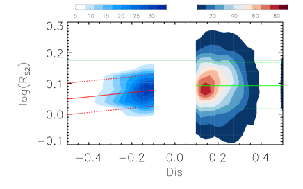
Third, dependence of $R_{S2}$ on distance $Dis$ of objects to the $R_{NLRs}-L_{O3}$ empirical relation in Liu et al. (2013) is checked for the 3658 Type-2 AGN in the Sample-II and the 1062 Type-2 AGN in the Sample-I, and shown in Fig. 6. Here, Type-2 AGN in Sample-II above the $R_{NLRs}-L_{O3}$ empirical relation have positive values of $Dis$, Type-2 AGN in Sample-I below the $R_{NLRs}-L$ empirical relation have negative values of $Dis$. For the Type-2 AGN in the Sample-II, there is no dependence of $R_{S2}$ on distance $Dis$, with calculated Spearman Rank correlation coefficient about 0.003 ($P_{null}\sim 0.84$). Therefore, if NLRs totally covered by SDSS fibers, no dependence of $R_{S2}$ on distance $Dis$ can be determined. Meanwhile, for the Type-2 AGN in the Sample-I, there is acceptable dependence of $R_{S2}$ on distance $Dis$: $\log(R_{S2})~{}\propto~{}0.07~{}\times~{}Dis$, with calculated Spearman Rank correlation coefficient about 0.16 ($P_{null}\sim 3\times 10^{-7}$). Therefore, the accepted dependence for the Type-2 AGN in the Sample-I but no dependence for the Type-2 AGN in the Sample-II can provide clues to support the basic point that whether NLRs totally covered by SDSS fibers can lead to statistically different properties of NLRs.

Fourth, as well discussed and shown in Osterbrock & Ferland (2006); Kewley et al. (2019b); Flury & Moran (2020); Zhang (2023), there are apparent effects of electron temperature on electron density estimated by $R_{S2}$, it is necessary to check whether are there different electron temperature properties for the Type-2 AGN in the Sample-I and in the Sample-II. Electron temperatures $T_{e}$ in AGN NLRs can be well traced by the emission line flux ratio $O_{32}$ of total [O iii]$\lambda 4959,5007$Å  to [O iii]4363Å. Unfortunately, as shown in Zhang (2023), not like [S ii] doublet commonly apparent in Type-2 AGN, only a small part of Type-2 AGN have apparent [O iii]$\lambda 4363$Å  emissions. Based on the ’GalSpecLine’ provided emission line fluxes and uncertainties of [O iii]4363Å  of the Type-2 AGN in the Sample-I and the Sample-II, there are only 7 of 3658 Type-2 AGN in the Sample-II and 289 of 1062 Type-2 AGN in Sample-I having their [O iii]$\lambda 4363$Å  emission fluxes at least five times larger than their uncertainties. Therefore, it is hard to provide statistical results on properties of $O_{32}$ of the Type-2 AGN in the Sample-I and in the Sample-II. However, simply qualitative discussions can be given as follows. Based on the electron temperature $T_{e}$ estimated through $O_{32}$

$$O_{32}~{}\propto~{}\exp(\frac{3.29\times 10^{4}}{T_{e}})$$ (3)

, quite weak [O iii]$\lambda 4363$Å  emissions (not apparent in SDSS spectra) in the Type-2 AGN in the Sample-II could indicate larger $O_{32}$, leading to lower electron temperature in NLRs for the Type-2 AGN in Sample-II than in Sample-I: $T_{e}(Sample-II)~{}<~{}T_{e}(sample-I)$. Meanwhile, accepted the dependence of electron density $n_{e}$ on $T_{e}$ and $R_{S2}$

$$\frac{n_{e}}{\rm cm^{3}}\times(\frac{10^{4}K}{T_{e}})^{0.5}~{}\approxeq~{}f(R_{S2})=\frac{627.1~{}\times~{}R_{S2}~{}-~{}909.17}{0.4315~{}-~{}R_{S2}}$$ (4)

, considering that the Type-2 AGN in the Sample-II having smaller $f(R_{S2})$ (larger $R_{S2}$) and smaller $T_{e}$ than the Type-2 AGN in the Sample-I, it is apparent that very larger electron density $n_{e}$ could be expected in NLRs of the Type-2 AGN in the Sample-I after considering effects of electron temperature on estimations of $n_{e}$ through $R_{S2}$, well consistent with expected result that higher electron densities in NLRs of the Type-2 AGN in the Sample-I than in the Sample-II.

Fifth, similar as done to check effects of different redshift distributions, effects of different $L_{O3}$ distributions are checked as follows. Left panel of Fig. 7 shows the $\log(L_{O3}/{\rm erg/s})$ distributions with the mean value about 40.72 of the 3658 Type-2 AGN in the Sample-II and with the mean value about 40.57 of the 1062 Type-2 AGN in the Sample-I, respectively. And through the Students t-statistic technique, the Type-2 AGN in the Sample-II and in the Sample-I have the same mean values with significance level only about $8\times 10^{-17}$, indicating it is necessary to check effects of different $L_{O3}$ distributions. Among the Type-2 AGN in the Sample-II and in the Sample-I, two subsamples, one subsample (subsample-II) including 1033 Type-2 AGN from the Sample-II and the other subsample (subsample-I) including 1033 Type-2 AGN from the Sample-I, can be simply created to have the same $\log(L_{O3})$ distributions with significance levels higher than 99.99% through the two-sided Kolmogorov-Smirnov statistic technique. The same $\log(L_{O3})$ distributions of Type-2 AGN in the new subsamples are shown in middle panel of Fig. 7. Meanwhile, right panel of Fig. 7 shows $\log(R_{S2})$ distributions of the Type-2 AGN in the two new subsamples. The median values and the corresponding bootstrap method determined uncertainties of $\log(R_{S2})$ (with $R_{S2}<1.5$) are about $(8.08\pm 0.14)\times 10^{-2}$ and $(6.71\pm 0.15)\times 10^{-2}$ for the Type-2 AGN in the new subsample-II and in the new subsample-I, respectively. And through the Wilcoxon Rank-Sum Test, the Type-2 AGN in the new subsample-II and in the new subsample-I have the same median values of $\log(R_{S2})$ (with $R_{S2}<1.5$) with significance level only about $10^{-15}$, to re-confirm higher $R_{S2}$ for the Type-2 AGN above the $R_{NLRs}-L_{O3}$ relation. Therefore, there are few effects of different $\log(L_{O3})$ distributions on different $\log(R_{S2})$ for the Type-2 AGN in the Sample-II and in the Sample-I.

Figure 10: Left panel shows the W2-W4 distributions of the Type-2 AGN in the Sample-II (histogram filled by blue lines) and in the Sample-I (histogram filled by red lines), respectively. Vertical blue line and red line in top region of left panel mark the mean values of W2-W4 of the Type-2 AGN in the Sample-II and in the Sample-I, respectively. Middle panel shows the W2-W4 distributions of the Type-2 AGN in the new subsamples which have the same W2-W4 distributions. Right panel shows the $\log(R_{S2})$ distributions of the Type-2 AGN in the new subsamples which have the same W2-W4 distributions. In the right panel, line styles have the same meanings as those in Figure 3.

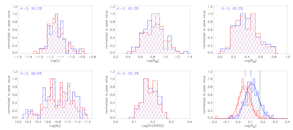
Sixth, due to the fixed fiber sizes for SDSS spectra, it is necessary to check whether the collected Type-2 AGN in different samples have intrinsically different host galaxy properties by the following collected parameters which could affect the results shown in Fig. 3. The parameters of petroR90_r and petroR50_r (as the radii containing 90% and 50% of the Petrosian flux in SDSS r-band photometric image) are collected from the public SDSS database ’PhotoObjAll’ which contains full photometric catalog quantities, in order to check effects of size ($R_{90}$ and $R_{50}$) of host galaxy. The parameter of d4000_n (the common parameter Dn(4000) as discussed in Kauffmann et al. 2003) are collected from the public SDSS database ’galSpecIndx’, in order to check effects of stellar ages of host galaxy. The parameter mstellar_median are collected from the public database ’stellarMassPCAWiscM11’ as described in Maraston & Stromback (2011); Chen et al. (2012), in order to check effects of total stellar mass $M_{*}$ of host galaxy. The detailed descriptions on the applied databases above can be found in https://skyserver.sdss.org/dr16/en/help/docs/tabledesc.aspx. Then, Fig. 8 shows the distributions of $R_{90}$, $R_{50}$, Dn(4000) and $M_{*}$ for the Type-2 AGN in the Sample-I and in the Sample-II, respectively, leading to clearly different distributions of the parameters of the Type-2 AGN in the different samples. In order to check the effects of the different distributions of the parameters shown above, a new subsmaple-I including 96 Type-2 AGN from the Sample-II and a new subsample-II including 96 Type-2 AGN from the Sample-I can be created to have the same distributions of redshift $z$, $R_{90}$, $R_{50}$, Dn(4000) and $M_{*}$. Here, combining with the same distributions of size of host galaxy, to also consider the same redshift distributions can be applied to ignore aperture effects. The first five panels of Figure 9 shows the same distributions of $z$, $R_{90}$, $R_{50}$, Dn(4000) and $M_{*}$ of the Type-2 AGN in the new subsamples. Through the two-sided Kolmogorov-Smirnov statistic technique, the 96 Type-2 AGN in the new subsample-II and the 96 Type-2 AGN in the new subsample-I have the same distributions of redshift, size of host galaxy, total stellar mass and stellar age, with significance levels higher than 95.3%. Here, the same distributions of $R_{90}$ and $R_{50}$ also indicate the similar distributions of inverse concentration parameter (Shimasaku et al., 2001; Strateva et al., 2001) to show not large difference of host galaxy morphology of the collected Type-2 AGN. Then, bottom right panel of Figure 9 shows the $R_{S2}$ distributions of the Type-2 AGN in the new subsamples. The median values and the corresponding bootstrap method determined uncertainties of $\log(R_{S2})$ (with $R_{S2}~{}<~{}1.5$) are about $(10.31\pm 0.28)\times 10^{-2}$ and $(5.68\pm 0.15)\times 10^{-2}$ for the Type-2 AGN in the new subsample-II and the Type-2 AGN in the new subsample-I, respectively. And through the Wilcoxon Rank-Sum Test, the Type-2 AGN in the subsample-II and in the subsample-I have significantly different median values of $\log(R_{S2})$ (with $R_{S2}~{}<~{}1.5$) with significance level about $10^{-13}$. Therefore, there are few effects of host galaxy properties on the different $\log(R_{S2})$ for the Type-2 AGN in the Sample-II and in the Sample-I.

Seventh, although we have simply accepted few effects of orientations on NLRs in Type-2 AGN considering the unified model of AGN, we should note that He et al. (2018) have discussed that structure properties of NLRs in Type-2 AGN could be shaped by obscurations. Therefore, it is necessary to check effects of obscurations traced by WISE mid-IR colors (W2-W4) as pointed in He et al. (2018). Then, through the SDSS public database ’WISE_allsky’, the photometric magnitudes in W2 and W4 bands are collected for the collected Type-2 AGN. Left panel of Fig. 10 shows the mid-IR color distributions of the Type-2 AGN, with the mean value of about 5.42 for the Type-2 AGN in the Sample-II and about 5.64 for the Type-2 AGN in the Sample-I. And through the Students t-statistic technique, the Type-2 AGN in the Sample-II and in the Sample-I have the same mean values of W2-W4 with significance level only about $2\times 10^{-2}$, indicating it is necessary to check effects of different W2-W4 distributions. Among the Type-2 AGN in the Sample-II and in the Sample-I, two subsamples, one subsample (subsample-II) including 1049 Type-2 AGN from the Sample-II and the other subsample (subsample-I) including 1049 Type-2 AGN from the Sample-I, can be simply created to have the same W2-W4 distributions with significance levels higher than 99.99% through the two-sided Kolmogorov-Smirnov statistic technique. The same W2-W4 distributions of Type-2 AGN in the new subsamples are shown in middle panel of Fig. 10. Meanwhile, right panel of Fig. 10 shows $\log(R_{S2})$ distributions of the Type-2 AGN in the two new subsamples. The median values and the corresponding bootstrap method determined uncertainties of $\log(R_{S2})$ (with $R_{S2}<1.5$) are about $(8.99\pm 0.15)\times 10^{-2}$ and $(6.81\pm 0.18)\times 10^{-2}$ for the Type-2 AGN in the new subsample-II and in the new subsample-I, respectively. And through the Wilcoxon Rank-Sum Test, the Type-2 AGN in the new subsample-II and in the new subsample-I have the same median values with significance level only about $10^{-11}$, to re-confirm higher $R_{S2}$ for the Type-2 AGN above the $R_{NLRs}-L_{O3}$ relation. Therefore, there are few effects of obscuration shaped NLRs structures on the different $\log(R_{S2})$ for the Type-2 AGN in the Sample-II and in the Sample-I.

Therefore, the results shown in Fig. 3 and Fig. 5 and corresponding discussions above can be applied to support the $R_{NLRs}-L_{O3}$ empirical relation reported in Liu et al. (2013) and also to support electron density gradients in AGN NLRs. Unfortunately, only through comparisons between $R_{fib}$ and $R_{NLRs}$, it is hard to estimate a clear quantitative result on the expected $R_{NLRs}-L_{O3}$ relation and the electron density gradients in AGN NLRs.

Before end of the subsection, three additional points are noted. First, besides the discuused median values of $\log(R_{S2})$ for the AGN in the different samples/subsamples, mean values of $\log(R_{S2})$ have also been checked, and the Students t-statistic technique can be applied to confirm the AGN in the different samples/subsamples having the very different mean values of $\log(R_{S2})$ with confidence levels higher than 5$\sigma$. Second, besides the discussed subsamples above with the same distributions of the pointed parameters, similar subsamples are also created with the same distributions of the same parameters, but with different objects included, after randomly shuffling the orders of the objects in the parent samples. Then, different subsamples with the same distributions of the given parameters lead to the very similar $\log(R_{S2})$ difference, to support few effects of the randomly collected objects on our final results. Third, besides the $R_{NLRs}-L_{O3}^{0.25}$ relation reported in Liu et al. (2013), the $R_{NLRs}-L_{O3}^{0.4\sim 0.5}$ relation discussed in Schmitt et al. (2003); Fischer et al. (2018); Chen et al. (2019) is also shown in Fig. 2. Unfortunately, in Fig. 2, there is only one Type-2 AGN lying below the $R_{NLRs}-L_{O3}$ relation minus 2RMS scatter reported in Schmitt et al. (2003); Fischer et al. (2018), and only four Type-2 AGN lying below the $R_{NLRs}-L_{O3}$ relation minus its corresponding 2RMS scatter reported in Chen et al. (2019). In other words, if accepted the $R_{NLRs}-L_{O3}$ relation reported in Schmitt et al. (2003); Fischer et al. (2018), almost all the collected SDSS Type-2 AGN have their NLRs totally covered by SDSS fibers, indicating similar properties of electron densities in NLRs of the Type-2 AGN in the Sample-I and in the Sample-II created above, against the shown results in Fig. 3. Therefore, rather than the $R_{NLRs}-L_{O3}^{0.4\sim 0.5}$ relation reported in Schmitt et al. (2003); Fischer et al. (2018); Chen et al. (2019), the $R_{NLRs}-L_{O3}^{0.25}$ relation reported in Liu et al. (2013) is the preferred empirical relation to estimate NLRs sizes of SDSS AGN through the [O iii] line luminosity measured from SDSS fiber optical spectroscopic results.

4 Summary and Conclusions

The main summary and conclusions are as follows.

• Considering AGN unified model expected spatial properties of NLRs of Type-2 AGN, SDSS fiber radii provided spatial distance $R_{fib}$ can be applied to test the $R_{NLRs}-L$ empirical relation to estimate NLRs sizes of AGN.

• Comparing $R_{fib}$ and $R_{NLRs}$ estimated through [O iii] line luminosity, Type-2 AGN in SDSS can be divided into two samples, one sample of Type-2 AGN with $R_{fib}>R_{NLRs}$ have their NLRs totally covered by SDSS fibers, the other sample of Type-2 AGN with $R_{fib}<R_{NLRs}$ have their NLRs partly covered by SDSS fibers.

• Considering expected electron density gradients in AGN NLRs, different physical properties of NLRs could be expected for Type-2 AGN with $R_{fib}>R_{NLRs}$ and for Type-2 AGN with $R_{fib}<R_{NLRs}$.

• Among the SDSS pipeline classified Type-2 AGN, after LINERs being removed, considering the $R_{NLRs}-L$ empirical relation and 2RMS scatters reported in Liu et al. (2013), 3658 Type-2 AGN with $R_{fib}>R_{NLRs}$ are collected and included in Sample-II, and 1062 Type-2 AGN $R_{fib}<R_{NLRs}$ are collected and included in Sample-I.

• There are statistically lower $R_{S2}$ (flux ratio of [S ii]$\lambda 6717$Å  to [S ii]$\lambda 6731$Å) for the Type-2 AGN in Sample-I than in Sample-II, with confidence level higher than 5$\sigma$.

• There are no different dependence of $R_{S2}$ on redshift for the Type-2 AGN in Sample-I and in Sample-II, indicating few effects of different redshift distributions on statistically lower $R_{S2}$ for the Type-2 AGN in Sample-I than in Sample-II.

• Through the Type-2 AGN in Sample-I and in Sample-II, two subsamples can be created to have the same redshift distributions. And statistically lower $R_{S2}$ can be confirmed for the Type-2 AGN in the subsample-I than in the subsample-II, to reconfirm few effects of different redshift distributions on statistically lower $R_{S2}$ for the Type-2 AGN in Sample-I than in Sample-II.

• Through the Type-2 AGN in Sample-I and in Sample-II, two subsamples can be created to have the same distributions of $z$, $R_{90}$, $R_{50}$, $M_{*}$ and Dn(4000) to check effects of host galaxy properties, to reconfirm the statistically lower $R_{S2}$ for the Type-2 AGN in Sample-I.

• Even after considering effects of obscurations traced by WISE mid-UR colors on shaped NLRs structures, through two subsamples with the same W2-W4 distributions, the statistically lower $R_{S2}$ can be reconfirmed for the Type-2 AGN in Sample-I.

• Considering NLRs partly covered by SDSS fibers for the Type-2 AGN in Sample-I, more apparently statistically lower intrinsic $R_{S2}$ could be expected for the Type-2 AGN in Sample-I.

• Different dependence of $R_{S2}$ on distance $Dis$ of objects to the $R_{NLRs}-L_{O3}$ empirical relation in Liu et al. (2013) can be found for the Type-2 AGN in Sample-I and in Sample-II, providing clues to support that the provided method in this manuscript can be efficiently applied to test the $R_{NLRs}-L_{O3}$ empirical relation.

• Statistically lower $R_{S2}$ for the Type-2 AGN in Sample-I can be applied to support the $R_{NLRs}-L_{O3}$ empirical relation in Liu et al. (2013) to estimate NLRs sizes of SDSS AGN, and also to support the commonly expected electron density gradients in AGN NLRs.

Data Availability

The data underlying this article will be shared on reasonable request to the corresponding author (xgzhang@gxu.edu.cn).

References

- Ahumada et al. (2020) Ahumada, R.; Prieto, C. A.; Almeida, A.; et al., 2020, ApJS, 249, 3
- Antonucci (1993) Antonucci, R., 1993, ARA&A, 31, 473
- Audibert et al. (2017) Audibert, A.; Riffel, R.; Sales, D. A.; Pastoriza, M. G.; Ruschel-Dutra, D., 2017, MNRAS, 464, 2139
- Baldwin et al. (1981) Baldwin, J. A.; Phillips, M. M.; Terlevich, R. 1981, PASP, 93, 5
- Balokovic et al. (2018) Balokovic, M.; Brightman, M.; Harrison, F. A.; et al., 2018, ApJ, 854, 42
- Bianchi et al. (2012) Bianchi, S.; Maiolino, R.; Risaliti, G., 2012, Advances in Astronomy, 2012, 17
- Brinchmann et al. (2004) Brinchmann, J.; Charlot, S.; White, S. D. M.; et al., 2004, MNRAS, 351, 1151
- Brown et al. (2019) Brown, A.; Nayyeri, H.; Cooray, A.; Ma, J.; Hickox, R. C.; Azadi, M, 2019, ApJ, 871, 87
- Chen et al. (2019) Chen, J. H.; Shi, Y.; Dempsey, R.; et al., 2019, MNRAS, 489, 855
- Chen et al. (2012) Chen, Y.; Kauffmann, G.; Tremonti, C. A.; et al., 2012, MNRAS, 421, 314
- Cid Fernandes et al. (2011) Cid Fernandes, R.; Stasinska, G.; Mateus, A.; et al., 2011, MNRAS, 413, 1687
- Dempsey & Zakamska (2018) Dempsey, R.; Zakamska, N. L., 2018, MNRAS, 477, 4615
- Dopita & Sutherland (1996) Dopita, M. A.; Sutherland, R. S., 1996, ApJS, 102, 161
- Dopita et al. (2015) Dopita, M. A.; Ho, I.-T.; Dressel, L. L., et al., 2015, ApJ, 801, 42
- Dors et al. (2022) Dors, O. L.; Valerdi, M.; Freitas-Lemes, P.; et al., 2022, MNRAS, 514, 5506
- Eracleous et al. (2010) Eracleous, M.; Hwang, J. A.; Flohic, H. M. L. G., 2010, ApJ, 711, 796
- Fischer et al. (2018) Fischer, Travis C.; Kraemer, S. B.; Schmitt, H. R.; et al., 2018, ApJ, 856, 102
- Filippenko & Terlevich (1992) Filippenko, A. V. & Terlevich, R., 1992, ApJL, 397, 79
- Flury & Moran (2020) Flury, S. R.; Moran, E. C., 2020, MNRAS, 496, 2191
- Gomez-Guijarro et al. (2017) Gomez-Guijarro, C.; Gonzalez-Martin, O.; Ramos Almeida, C.; Rodrrguez-Espinosa, J. M.; Gallego, J., 2017, MNRAS, 469, 272
- Hainline et al. (2013) Hainline, K. N.; Hickox, R. C.; Greene, J. E.; Myers, A. D.; Zakamska, N. L., 2013, ApJ, 774, 145
- Hainline et al. (2014) Hainline, K. N.; Hickox, R. C.; Greene, J. E.; Myers, A. D.; Zakamska, N. L.; Liu, G.; Liu, X., 2014, ApJ, 787, 65
- He et al. (2018) He, Z. C.; Sun, A. L., Zakamska, N. L.; et al., 2018, MNRAS, 478, 3614
- Heckman (1980) Heckman, T. M., 1980, A&A, 87, 152
- Husemann et al. (2022) Husemann, B.; Singha, M.; Scharwachter, J.; et al., 2022, A&A, 659, 124
- Kakkad et al. (2018) Kakkad, D.; Groves, B.; Dopita, M.; et al., 2018, A&A, 618, 6
- Kauffmann et al. (2003a) Kauffmann, G.; Heckman, T. M.; White, S. D. M.; et al., 2003a, MNRAS, 341, 33
- Kauffmann et al. (2003) Kauffmann, G.; Heckman, T. M.; Tremonti, C.; et al. 2003, MNRAS, 346, 1055
- Kawasaki et al. (2017) Kawasaki, K.; Nagao, T.; Toba, Y.; Terao, K.; Matsuoka, K., 2017, ApJ, 842, 44
- Kazuma et al. (2021) Kazuma, J.; Nagao, T.; Wada, K.; Koki Terao, K.; Takuji, Y., 2021, PASJ, 73, 1152
- Kewley et al. (2001) Kewley, L. J.; Dopita, M. A.; Sutherland, R. S.; Heisler, C. A.; Trevena, J. 2001, ApJ, 556, 121
- Kewley et al. (2006) Kewley, L. J.; Groves, B.; Kauffmann, G.; Heckman, T., 2006, MNRAS, 372, 961
- Kewley et al. (2019a) Kewley, L. J.; Nicholls, D. C.; Sutherland, R. S., 2019a, ARA&A, 57, 511
- Kewley et al. (2019b) Kewley, L. J.; Nicholls, D. C.; Sutherland, R.; et al., 2019b, ApJ, 880, 16
- Kuraszkiewicz et al. (2021) Kuraszkiewicz, J.; Wilkes, B. J.; Atanas, A.; et al., 2021, ApJ, 913, 134
- Liu et al. (2013) Liu, G. L.; Zakamska, N. L.; Greene, J. E.; Nesvadba, N. P. H.; Liu, X., 2013, MNRAS, 430, 2327
- Maraston & Stromback (2011) Maraston, C.; Stromback, G., 2011, MNRAS, 418, 2785
- Marquez et al. (2017) Marquez I.; Masegosa J.; Gonzalez-Martin O.; et al., 2017, Frontiers in Astronomy and Space Sciences, 4, 34
- Marinucci et al. (2012) Marinucci, A.; Bianchi, S.; Nicastro, F.; Matt, G.; Goulding, A. D., 2012, ApJ, 748, 130
- Mateos et al. (2016) Mateos, S.; Carrera, F. J.; Alonso-Herrero, A.; et al., 2016, ApJ, 819, 166
- Meena et al. (2023) Meena, B.; Crenshaw, D. M.; Schmitt, H. R.; et al., 2023, ApJ, 943, 78
- Mignoli et al. (2019) Mignoli, M.; Feltre, A.; Bongiorno, A.; et al., 2019, A&A, 626, 9
- Netzer & Laor (1993) Netzer, H.; Laor, A., 1993, ApJL, 404, 51
- Netzer et al. (2004) Netzer, H.; Shemmer, O.; Maiolino, R.; Oliva, E.; Croom, S.; Corbett, E.; di Fabrizio, L., 2004, ApJ, 614, 558
- Netzer (2015) Netzer, H., 2015, ARA&A, 53, 365
- Oh et al. (2015) Oh, K.; Yi, S. K.; Schawinski, K.; Koss, M.; Trakhtenbrot, B.; Soto, K., 2015, ApJS, 219, 1
- Osterbrock & Ferland (2006) Osterbrock, D. E.; Ferland, G. J., 2006, Astrophysics of gaseous nebulae and active galactic nuclei, 2nd. ed., CA: University Science Books
- Riffel et al. (2021) Riffel R. A.; Dors, O. L.; Armah, M.; et al., 2021, MNRAS, 501, L54
- Sanders et al. (2016) Sanders, R. L.; Shapley, A. E.; Kriek, M.; et al. 2016, ApJ, 816, 23
- Schmitt et al. (2003) Schmitt, H. R.; Donley, J. L.; Antonucci, R. R. J.; Hutchings, J. B.; Kinney, A. L., 2003, ApJS, 148, 327
- Shimasaku et al. (2001) Shimasaku, K.; Fukugita, M.; Doi, M.; et al., 2001, ApJ, 122, 1238
- Strateva et al. (2001) Strateva, I.; Ivezic, Z.; Knapp, G. R.; et al., 2001, AJ, 122, 1861
- Shen et al. (2011) Shen, Y.; Richards, G. T.; Strauss, M. A., et al., 2011, ApJS, 194, 45
- Stoklasova et al. (2009) Stoklasova, I.; Ferruit, P.; Emsellem, E.; Jungwiert, B.; Pecontal, E.; Sanchez, S. F., 2009, A&A, 500, 287
- Sun et al. (2018) Sun, A. L.; Greene, J. E.; Zakamska, N. L.; et al., 2018, MNRAS, 480, 2302
- Thomas et al. (2018) Thomas, A. D.; Dopita, M. A.; Kewley, L. J.; Groves, B. A.; Sutherland, R. S.; Hopkins, A. M.; Blanc, G. A., 2018, ApJ, 856, 89
- Tremonti et al. (2004) Tremonti, C. A.; Heckman, T. M.; Kauffmann, G.; et al., 2004, ApJ, 613, 898
- Zhang et al. (2020) Zhang, X. G.; Feng Y.; Chen, H.; Yuan, Q., 2020, ApJ, 905, 97
- Zhang (2022) Zhang, X. G., 2022, ApJS, 260, 31, arXiv:2203.12810
- Zhang (2023) Zhang, X. G., 2023, ApJ accepted, arXiv:2309.00852