Acquiring Clean Language Models from Backdoor Poisoned Datasets by Downscaling Frequency Space

Abstract

Despite the notable success of language models (LMs) in various natural language processing (NLP) tasks, the reliability of LMs is susceptible to backdoor attacks. Prior research attempts to mitigate backdoor learning while training the LMs on the poisoned dataset, yet struggles against complex backdoor attacks in real-world scenarios. In this paper, we investigate the learning mechanisms of backdoor LMs in the frequency space by Fourier analysis. Our findings indicate that the backdoor mapping presented on the poisoned datasets exhibits a more discernible inclination towards lower frequency compared to clean mapping, resulting in the faster convergence of backdoor mapping. To alleviate this dilemma, we propose Multi-Scale Low-Rank Adaptation (MuScleLoRA), which deploys multiple radial scalings in the frequency space with low-rank adaptation to the target model and further aligns the gradients when updating parameters. Through downscaling in the frequency space, MuScleLoRA encourages the model to prioritize the learning of relatively high-frequency clean mapping, consequently mitigating backdoor learning. Experimental results demonstrate that MuScleLoRA outperforms baselines significantly. Notably, MuScleLoRA reduces the average success rate of diverse backdoor attacks to below 15% across multiple datasets and generalizes to various backbone LMs, including BERT, RoBERTa, and Llama2. The codes are available at https://github.com/ZrW00/MuScleLoRA.git.

Acquiring Clean Language Models from Backdoor Poisoned Datasets by Downscaling Frequency Space

Zongru Wu, Zhuosheng Zhang, Pengzhou Cheng, Gongshen Liu School of Cyber Science and Engineering, Shanghai Jiao Tong University {wuzongru, zhangzs, cpztsm520, lgshen}@sjtu.edu.cn

1 Introduction

Despite the remarkable achievements of language models (LMs) in various natural language processing (NLP) tasks (Devlin et al., 2019; Touvron et al., 2023), concerns arise due to the lack of interpretability in the internal mechanisms of LMs, impacting their reliability and trustworthiness. A particular security threat to LMs is backdoor attack (Liu et al., 2018; Chen et al., 2017). Backdoor attack poisons a small portion of the training data by implanting specific text patterns (known as triggers). Trained on the poisoned dataset, the target LM performs maliciously when processing samples containing the triggers, while behaving normally when processing clean text.

Prior works attempt to mitigate backdoor learning during training the target LM on the poisoned dataset (Zhu et al., 2022; Zhai et al., 2023). However, due to the stealthy nature of complex triggers in real-world scenarios, most existing defense methods fail to mitigate backdoor learning from such triggers, like specific text style (Qi et al., 2021b) or syntax (Qi et al., 2021c). To better understand backdoor learning, we explore the learning mechanisms of LMs in the frequency space on the poisoned datasets through Fourier analysis. The findings indicate that the backdoor mapping presented on the poisoned datasets exhibits a stronger inclination towards lower frequency compared to clean mapping. According to the extensively studied F-Principle (Xu et al., 2020; Xu and Zhou, 2021; Rahaman et al., 2019), which suggests that deep neural networks (DNNs) tend to fit the mapping from low to high frequency during training, these results explain why backdoor mapping is notably easier to discern and converges faster for LMs.

Inspired by the observation and thought above, we propose a general backdoor defense method named Multi-Scale Low-Rank Adaptation (MuScleLoRA) to further mitigate backdoor learning. MuScleLoRA integrates multiple radial scalings in the frequency space with low-rank adaptation to the target LM and aligns gradients during parameter updates. By downscaling in the frequency space, MuScleLoRA encourages LMs to prioritize relatively high-frequency clean mapping, thereby mitigating learning the backdoor on the poisoned dataset while enhancing clean learning. Experimental results across multiple datasets and model architectures demonstrate the efficacy and generality of MuScleLoRA in defending against diverse backdoor attacks compared to baselines.

Specifically, we concentrate on the scenario where (1) the attacker poisons and releases the dataset on open third-party platforms, without gaining control of the downstream training; (2) the defender downloads the poisoned dataset and deploys the defense method to train the target LM, maintaining complete control of the training process. Our contributions are summarized as follows:

(1) We conduct Fourier analyses to investigate the mechanisms of backdoor learning, revealing why backdoor mapping is notably easier to discern for LMs compared to clean mapping. To the best of our knowledge, this is the first work that explores the mechanisms of backdoor learning from the perspective of Fourier analysis and transfers these insights into backdoor defense strategies.

(2) Inspired by our findings in the frequency space, we propose a general backdoor defense method named MuScleLoRA, which integrates multiple radial scalings in the frequency space with low-rank adaptation to the target LM, and further aligns the gradient when updating parameters.

(3) We conduct experiments across several datasets and model architectures, including BERT, RoBERTa, and Llama2, to validate the efficacy and generality of MuScleLoRA in backdoor mitigation. Compared to baseline methods, MuScleLoRA consistently demonstrates its capability to effectively defend against diverse backdoor attacks.

2 Related Works

In this section, we cover related works that form the basis of this work from four perspectives: backdoor attack, backdoor defense, learning mechanisms of DNNs, and parameter-efficient tuning (PET).

Backdoor Attack. Backdoor learning seeks to exploit the extra capacity (Zhu et al., 2023) of over-parameterized (Han et al., 2016) LMs to establish a robust mapping between predefined triggers and the target label. One typical way to conduct backdoor attacks is dataset poisoning (Chen et al., 2017). Recent studies for trigger implantation include inserting specific words (Kurita et al., 2020) or sentences (Dai et al., 2019) that use shallow semantic features. Additionally, high-level semantics, like specific syntax (Qi et al., 2021c) and text style (Qi et al., 2021b), are utilized as complex triggers.

Backdoor Defense. Backdoor defense aims to mitigate potential backdoors in victim LMs and is categorized into training-stage and post-training defense. During training, the defender can perform poisoned weight removal (Zhang et al., 2022, 2023c; Liu et al., 2023), regularized training (Zhu et al., 2022; Zhai et al., 2023), and dataset purifying (Chen and Dai, 2021; Cui et al., 2022; Jin et al., 2022) to mitigate backdoor learning. After training, the defender can employ trigger inversion Azizi et al. (2021); Shen et al. (2022); Liu et al. (2022), trigger detection Qi et al. (2021a); Shao et al. (2021), and poison input detection Gao et al. (2021); Yang et al. (2021) to discriminate potential backdoors. Our proposed MuScleLoRA falls under regularized training, mitigating backdoor learning without detailed inspection of data distribution. Previous work (Zhu et al., 2022) attempts to reduce the model capacity by PET methods to mitigate backdoor learning. However, straightforward model capacity reduction with PET methods requires meticulously designed hyperparameters against different attacks and still struggles against complex stealthy triggers, like specific syntax Qi et al. (2021c).

Learning Mechanisms of DNNs and Backdoor LMs. Extensive research focuses on revealing the learning mechanisms of DNNs. Recent studies shed light on these mechanisms through Fourier analysis (Rahaman et al., 2019). By transforming the input-output mapping into the frequency space, the findings suggest that, owing to the decay of activation functions in the frequency space (Xu et al., 2020), DNNs tend to fit the mapping from low to high frequency during training. Besides, deeper DNNs exhibit a stronger low-frequency bias (Xu and Zhou, 2021). Empirical studies also confirm that backdoor learning converges notably faster than clean mapping (Li et al., 2021; Gu et al., 2023; Zhang et al., 2023b), hinting at a low-frequency bias of the backdoor in the frequency space.

Parameter-Efficient Tuning. Recently, PET emerges as a novel training paradigm for LMs. PET achieves comparable performance to fine-tuning by freezing the original parameters and introducing tunable modules with fewer parameters, such as parallel low-rank decompositions (Hu et al., 2022), sequential linear layers Houlsby et al. (2019), and a sequence of continuous task-specific vectors (Li and Liang, 2021). Consequently, PET can reduce the extra capacity of LMs, thereby partially mitigating backdoor learning (Zhu et al., 2022).

3 Pilot Experiments

In this section, we conduct pilot experiments on the poisoned dataset, investigating the learning mechanisms of LMs in the frequency space from the perspective of Fourier analysis.

Intuitively, the implanted triggers on the poisoned dataset represent a straightforward recurring feature that LMs can easily discern. A recent empirical study observes faster convergence of backdoor mapping loss compared to clean mapping during training LM on the poisoned dataset (Gu et al., 2023). To explain this observed convergence difference, we conduct Fourier analyses on the training process of the backdoor LM.

Following the settings of Kurita et al. (2020) and Dai et al. (2019), we select specific words, i.e., cf, mn, bb, tq, and a sentence, i.e., I watch this 3D movie, as respective triggers to poison SST-2 (Socher et al., 2013). We choose $\text{BERT}_{\text{Base}}$ as the target LM and train it on the poisoned datasets. Concurrently, we conduct filtering-based Fourier transformation (Xu et al., 2020) (details are provided in Appendix A) to the mapping $\mathcal{F}:\mathbb{R}^{L\times d}\to\mathbb{R}^{C},\mathcal{F}(e)=y$ that the LM fits during training. Here $e\in\mathbb{R}^{L\times d}$, $y\in\mathbb{R}^{C}$, $L$, $d$, and $C$ denote input embedding, output logits, input text length, embedding dimension, and the number of categories, respectively. We decompose the mapping into clean mapping and backdoor mapping by utilizing clean and poisoned inputs, extracting their respective low-frequency part $y^{\text{low}}_{\text{clean}},y^{\text{low}}_{\text{backdoor}}\in\mathbb{R}^{C}$ and high-frequency part $y^{\text{high}}_{\text{clean}},y^{\text{high}}_{\text{backdoor}}\in\mathbb{R}^{C}$.

(a) Specific Words

(b) Specific Sentence

Figure 1: Frequency ratios of clean and backdoor mapping during training $\text{BERT}_{\text{Base}}$ on poisoned SST-2.

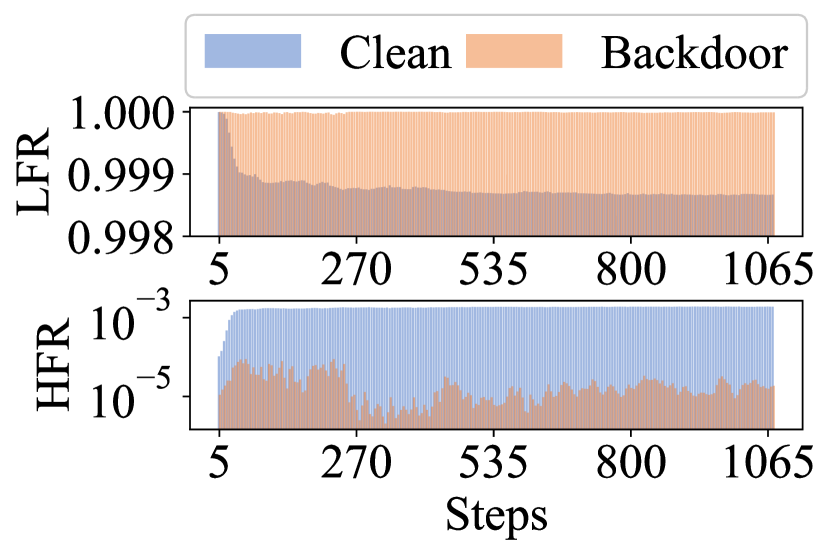
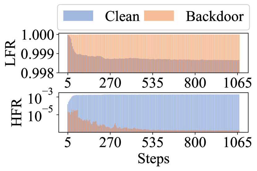
First, we calculate the low-frequency ratio (LFR) and high-frequency ratio (HFR) of both clean and backdoor mappings during training by Equation 1.

$$\text{LFR}=\frac{\|y^{\text{low}}\|}{\|y\|},\quad\text{HFR}=\frac{\|y^{\text{high}}\|}{\|y\|}.$$ (1)

As shown in Figure 1, both clean and backdoor mappings exhibit significantly larger LFR compared to HFR, consistent with the low-frequency bias suggested by F-Principle (Xu et al., 2020). Specifically, the LFR of backdoor mapping consistently remains near 1.0, surpassing that of clean mapping. Conversely, the HFR of clean mapping gradually increases, whereas the HFR of backdoor mapping is typically two orders of magnitude lower than that of clean mapping. These phenomena indicate that (1) backdoor mapping exhibits a stronger bias towards low frequency than clean mapping; (2) the high-frequency composition of backdoor mapping is negligible compared to clean mapping, which gradually acquires high-frequency information during training.

To compare the convergence of clean and backdoor mappings in frequency space, we compute the relative errors $\textrm{re}^{\text{low}},\textrm{re}^{\text{high}}$ between output logits and ground-truth labels by Equation 2. Here, $t^{\text{low}},t^{\text{high}}\in\mathbb{R}^{d}$ denote the low and the high frequency part of ground-truth mapping, respectively.

$$\textrm{re}^{\text{low}} =\frac{\|y^{\text{low}}-t^{\text{low}}\|}{\|t^{\text{low}}\|},$$ (2)

$$\textrm{re}^{\text{high}} =\frac{\|y^{\text{high}}-t^{\text{high}}\|}{\|t^{\text{high}}\|}.$$

(a) Specific words

(b) Specific Sentence

Figure 2: Relative errors of clean and backdoor mapping during training $\text{BERT}_{\text{Base}}$ on poisoned SST-2.

Figure 3: Overview of MuScleLoRA. MuScleLoRA is deployed while training the LM on the attacker-released poisoned dataset. We first freeze the target LM and insert LoRA modules into each attention layer. Subsequently, multiple radial scalings are conducted within the LoRA module at the penultimate layer of the target LM to downscale clean mapping. Additionally, we align gradients to the clean auxiliary data. These strategies encourage the target LM to prioritize the learning of high-frequency clean mapping, thereby mitigating backdoor learning.

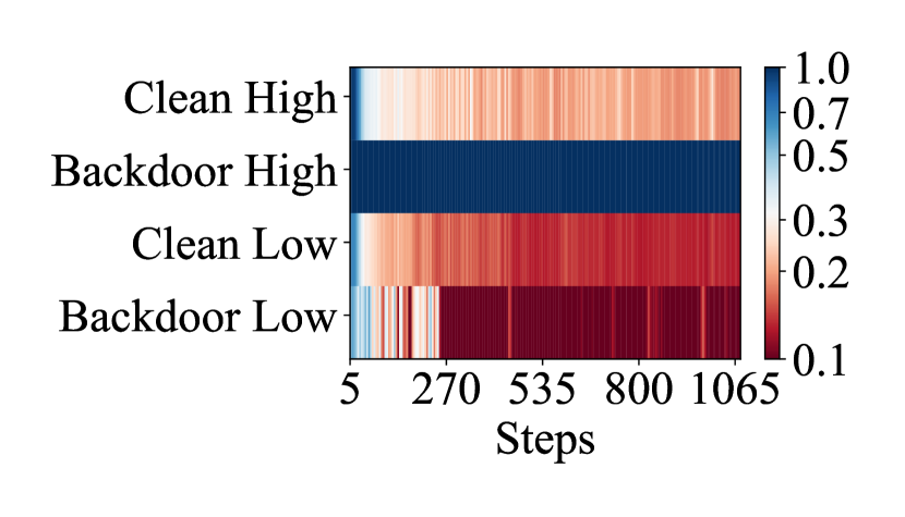
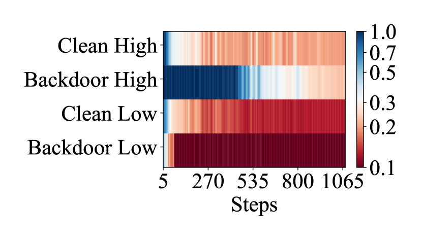
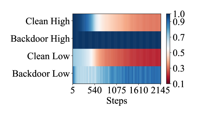
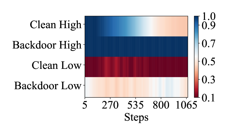
The results of relative errors are shown in Figure 2, where the red color indicates small relative errors. In both cases, $\textrm{re}^{\text{low}}$ decreases more rapidly than the corresponding $\textrm{re}^{\text{high}}$, signifying faster convergence. This convergence difference aligns with the Frequency Principle, suggesting that LMs tend to fit the mapping from low to high frequency. Furthermore, $\textrm{re}^{\text{low}}$ of low-frequency-dominated backdoor mapping fluctuates initially and then rapidly decreases to a small value. Compared to the gradual decrease of $\textrm{re}^{\text{low}}$ of clean mapping, backdoor mapping converges significantly faster. As mentioned above, (1) the lower-frequency inclination of backdoor mapping results in faster convergence of backdoor mapping, (2) the relatively high-frequency inclination of clean mapping leads to slower convergence of clean mapping.

4 Methodology

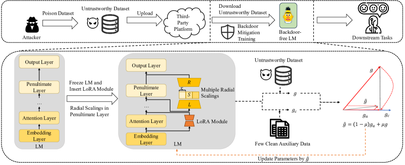
Findings in Section 3 indicate that clean mapping exhibits a relatively high-frequency bias, leading to its slower learning compared to backdoor mapping. Hence, an intuition to mitigate backdoor learning is to encourage LMs to prioritize relatively high-frequency clean mapping. To this end, we propose MuScleLoRA, which utilizes multiple radial scalings with low-rank adaptation to the target LM and aligns gradients when updating parameters. The overview of MuScleLoRA is shown in Figure 3.

Inspired by Zhu et al. (2022) that PET methods can reduce the capability of LM and thus mitigate backdoor learning, we incorporate multiple radial scalings (Liu et al., 2020) with low-rank adaptation to reduce the model capacity and downscale clean mapping in the frequency space.

For simplicity, we assume the Fourier transform $\hat{\mathcal{F}}_{\ell}(\xi),\xi\in\mathbb{R}^{d}$ corresponding to the mapping $\mathcal{F}_{\ell}(x),x\in\mathbb{R}^{d}$ fitted by the $\ell$th layer of LM has a compact support. Subsequently, the compact support of $\hat{\mathcal{F}}_{\ell}(\xi)$ can be partitioned into $s$ mutually disjointed concentric rings $\{A_{i}\}_{i=1}^{s},\forall i\neq j,A_{i}\cap A_{j}=\emptyset$. Therefore, $\hat{\mathcal{F}}_{\ell}(\xi)$ can be decomposed with indicators $\mathcal{I}(\xi\in A_{i})$, as illustrated in Equation 3.

$$\hat{\mathcal{F}}_{\ell}(\xi)=\sum_{i=1}^{s}\mathcal{I}(\xi\in A_{i})\hat{\mathcal{F}}_{\ell}(\xi)\triangleq\sum_{i=1}^{s}\hat{\mathcal{F}}_{\ell}^{i}(\xi).$$ (3)

For each $\hat{\mathcal{F}}_{\ell}^{i}(\xi)$, we apply radial scalings with appropriate scaling factor $s_{i}$ to downscale high frequency in $A_{i}$, as illustrated in Equation 4.

$$\hat{\mathcal{F}}_{\ell}^{\text{scale},i}(\xi)=\hat{\mathcal{F}}_{\ell}^{i}(s_{i}\xi).$$ (4)

Hence, in the corresponding physical space, the radial scalings are illustrated in Equation 5.

$$\mathcal{F}^{\text{scale},i}_{\ell}(x) =\mathcal{F}^{i}_{\ell}(\frac{1}{s_{i}}x),$$ (5)

$$\text{or}\quad\mathcal{F}^{i}_{\ell}(x) =\mathcal{F}^{\text{scale},i}_{\ell}(s_{i}x).$$

Consequently, $\mathcal{F}_{\ell}(x)$ can also be decomposed into: $\mathcal{F}_{\ell}(x)=\sum_{i=1}^{s}\mathcal{F}^{\text{scale},i}_{\ell}(s_{i}x)$. To approximate $\mathcal{F}^{\text{scale},i}_{\ell}$ with low-rank adaptation, we first freeze the target LM and insert LoRA modules into each attention Layer. Given that deeper layers tend to exhibit stronger low-frequency bias (Xu and Zhou, 2021), larger scaling factors are required in the shallow layers to appropriately downscale clean tasks. However, in practice, excessive scaling factors could potentially lead to underfitting.

Therefore, we conduct multiple radial scalings with appropriate scaling factors to the low-rank projected input $Lx$ within the LoRA module at the penultimate linear layer, as illustrated in Equation 6. Here, $W_{0}\in\mathbb{R}^{d\times d}$ denotes the original frozen weight, $R\in\mathbb{R}^{d\times sr}$ and $L\in\mathbb{R}^{sr\times d}$ denote the tunable low-rank decompositions with $sr\ll d$, $S\in\mathbb{R}^{sr}$ denotes the vector of scaling factors with bandwidth $r$ for each $A_{i}$, and $\odot$ denotes Hadamard product. Like vanilla LoRA, the magnitude of parameter updates can be represented as $R\left(L\odot S\right)$, which can be directly added to the original weights to mitigate the inference latency.

$$h =W_{0}x+\Delta Wx$$ (6)

$$=W_{0}x+R\left(Lx\odot S\right)$$

$$=W_{0}x+R\left(L\odot S\right)x.$$

As the relatively high-frequency clean mapping is downscaled by multiple radial scalings in the frequency space, the inclination towards the low-frequency-dominated backdoor mapping is mitigated. Therefore, with the low-rank adaptation that reduces the model capacity, the target LM is likely to prioritize the more general clean mapping on the poisoned dataset.

However, with the burgeoning scale of LMs, the accompanying increase in extra capacity of LMs poses challenges to effectively mitigate backdoor learning through straightforward model capacity reduction with PET methods. Motivated by the notable phenomenon that the gradient directions derived from poisoned data and clean data often conflict with each other (Kurita et al., 2020; Gu et al., 2023), we assume the defender can access a small amount of clean auxiliary data, usually comprising a few dozen instances and readily obtainable through manual labeling. Consequently, we align the gradient of the target LM with clean auxiliary data to further mitigate the influence of the poisoned gradient.

Specifically, when obtaining the original gradient $g$ from a batch of untrustworthy training data, we simultaneously calculate the clean gradient $g_{c}$ from a batch of clean auxiliary data. Subsequently, we align $g$ to the direction of $g_{c}$ to obtain the aligned gradient $g_{a}$, as illustrated in Equation 7:

$$g_{a}=\frac{\lvert g\cdot g_{c}\rvert}{\|g_{c}\|^{2}}g_{c}.$$ (7)

Nonetheless, aligning gradients to a restricted set of clean auxiliary data, as indicated by Chen et al. (2020), may lead to suboptimal learning. Therefore, we incorporate a fraction of the original gradient $g$ to mitigate suboptimal learning on clean tasks, as illustrated in Equation 8. Here, the hyperparameter $\mu$ denotes the ratio of the original gradient accepted. Subsequently, parameter updates are performed based on the modified gradient $\hat{g}$:

$$\hat{g}=(1-\mu)g_{a}+\mu g.$$ (8)

Practically, we linearly increase $\mu$ from 0 to the maximum value $\mu_{\max}$ throughout the training epochs. Consequently, the target LM primarily learns from backdoor-mitigated gradients during the early training phase, where $\mu$ approaches 0, and gradually incorporates more information with increasing $\mu$ to alleviate suboptimal learning in the later stages of training.

5 Experiments

In this section, we extensively evaluate MuScleLoRA. We first outline the setup in Section 5.1. Subsequently, in Section 5.2, we demonstrate that MuScleLoRA outperforms baselines significantly in backdoor mitigation across several datasets. Additionally, we analyze the contributions of various strategies employed in MuScleLoRA in Section 5.3, conduct Fourier analyses to explain the mechanisms of MuScleLoRA in the frequency space in Section 5.4, and extend MuScleLoRA to large language models (LLMs) in Section 5.5.

5.1 Experiment Setup

Datasets.

We conduct experiments on three sentence-level datasets: SST-2 (Socher et al., 2013), HSOL (Davidson et al., 2017), and Agnews (AG) (Zhang et al., 2015), and one paragraph-level dataset: Lingspam (LS) (Sakkis et al., 2003). Dataset statistics are provided in Appendix B.1.

The Target LMs.

We choose BERT (Devlin et al., 2019) and RoBERTa (Liu et al., 2019), both with million-level parameters, and $\text{Llama2}_{\text{7B}}$ for classification (Touvron et al., 2023) with billion-level parameters, as the target LMs.

Dataset	Attack	Vanilla		LoRA		Adapter		Prefix		MuscleLoRA
		CACC$\uparrow$	ASR$\downarrow$	CACC$\uparrow$	ASR$\downarrow$	CACC$\uparrow$	ASR$\downarrow$	CACC$\uparrow$	ASR$\downarrow$	CACC$\uparrow$	ASR$\downarrow$
SST-2	Badnets	91.27	94.63	89.07	65.57	87.26	55.26	90.17	86.73	86.54	12.94
	Addsent	90.99	99.89	88.96	96.16	86.88	87.83	89.46	99.89	86.77	18.97
	HiddenKiller	91.10	93.53	88.58	52.96	86.60	45.39	88.52	68.64	87.64	25.11
	StyleBkd	91.71	77.19	88.91	57.24	87.10	60.96	90.06	63.60	87.81	33.22
HSOL	Badnets	93.24	98.39	91.99	54.18	85.80	49.60	94.45	73.67	86.00	24.31
	Addsent	92.27	100	90.82	93.16	83.62	67.31	93.80	100	85.47	2.74
	HiddenKiller	92.13	97.66	89.58	72.22	84.55	49.92	93.80	88.16	86.84	13.45
	StyleBkd	94.81	68.92	90.06	49.85	84.71	46.70	93.24	43.72	86.64	10.63
LS	Badnets	99.65	3.31	85.17	0	86.55	2.69	96.03	2.27	91.89	0
	Addsent	99.65	86.11	90.34	1.24	85.69	7.45	90.51	4.35	90.68	1.24
	HiddenKiller	99.31	98.97	92.93	27.69	83.79	1.05	96.21	86.92	95.52	0.20
	StyleBkd	98.96	92.24	95.17	37.10	84.66	2.10	93.79	8.59	93.96	4.28
AG	Badnets	92.80	51.25	89.59	3.28	89.64	2.56	90.85	50.37	87.74	2.35
	Addsent	92.75	100	89.05	100	89.21	100	90.58	100	87.72	3.90
	HiddenKiller	92.78	99.47	89.01	98.16	88.86	93.75	90.62	98.75	86.05	17.02
	StyleBkd	92.06	87.59	88.39	77.76	89.03	50.18	90.00	78.69	87.97	2.67

Table 1: Backdoor mitigation performance of MuScleLoRA and PET baselines when adopting $\text{BERT}_{\text{Base}}$ as the target LM on SST-2, HSOL, Lingspam, and Agnews. Vanilla denotes no defense deployment, and bold values indicate optimal ASRs.

Defense Baselines.

Following the settings of Zhu et al. (2022), we choose three PET methods as the baselines of model capacity reduction: LoRA (Hu et al., 2022), Adapter Houlsby et al. (2019), and Prefix-Tuning (Prefix) (Li and Liang, 2021). Additionally, we choose three post-training defense methods: ONION (Qi et al., 2021a), STRIP (Gao et al., 2021), and RAP (Yang et al., 2021), and two training-stage defense methods: BKI (Chen and Dai, 2021) and CUBE (Cui et al., 2022), as end-to-end defense baselines. Detailed descriptions of defense baselines are provided in Appendix B.2.

Attack Methods.

We adopt Badnets, which inserts specific words as triggers (Kurita et al., 2020), Addsent, which inserts a specific sentence as triggers (Dai et al., 2019), HiddenKiller, which paraphrases the original text into specific syntax as triggers (Qi et al., 2021c), and SytleBkd, which paraphrases the original text into specific text styles as triggers (Qi et al., 2021b). Notably, we paraphrase each sentence in the sample paragraph to implant triggers into the paragraph-level Lingspam dataset. All target labels are set to 1. Detailed trigger settings are provided in Appendix B.3.

Implementation Details.

To obtain clean auxiliary data, we randomly select a subset from the validation dataset. Additionally, following the observation that reducing the training epochs can mitigate backdoor learning (Zhu et al., 2022), we set training epochs to 10 for BERT and RoBERTa, and 5 for $\text{Llama2}_{\text{7B}}$. The default poison ratio is set to 0.1. Hyperparameters are unified across diverse attacks for each specific LM. More detailed hyperparameter settings are provided in Appendix B.4.

Metrics. We adopt clean accuracy (CACC) to evaluate the impact of the defense method on the clean dataset, where higher CACC indicates less negative impact. Additionally, we adopt attack success rate (ASR) to evaluate the defense performance on the poisoned dataset, where lower ASR signifies better performance in backdoor mitigation.

5.2 Performance in Backdoor Mitigation

The backdoor mitigation performances of MuscleLoRA and PET baselines on $\text{BERT}_{\text{Base}}$ are presented in Table 1. More results and analysis of backdoor mitigation performance on $\text{BERT}_{\text{Large}}$ and RoBERTa are provided in Appendix C.1.

Without any defense, four attack methods consistently achieve high CACC and ASR across several datasets, except for Badnets on Lingspam and Agnews. This discrepancy may be due to the excessive text length in Lingspam and the multi-class mapping in Agnews, which potentially hinder the establishment of backdoor mapping between specific words and the target label. Besides, StyleBkd exhibits relatively lower ASR compared to Addsent and HiddenKiller, likely due to the highly stealthy nature of the specific text style, making the establishment of backdoor mapping more challenging.

For PET baselines, the ASR for word-level Badnets drops by more than 30% in some datasets. However, PET baselines struggle against complex and stealthy triggers due to the absence of a strong constraint on clean mapping. Adapter can reduce ASR for all attack methods to less than 10% on Lingspam, but at the cost of unacceptable CACC. Since Lingspam consists of long texts, this phenomenon may be attributed to underfitting resulting from the limited number of training epochs and the small bottleneck dimension of PET modules.

Notably, compared to PET baselines, MuScleLoRA generally achieves the lowest ASR for all attack methods while maintaining acceptable CACCs across four datasets, especially on Lingspam, where the ASR drops to less than 5% while consistently preserving CACC above 90%. These results confirm that MuScleLoRA is highly effective in defending against complex triggers and significantly outperforms PET baselines.

We further compare the backdoor mitigation performance of MuScleLoRA with several end-to-end defense baselines mentioned in Section 5.1. The experimental results presented in Table 2 indicate that despite end-to-end baselines notably reducing ASR for Addsent, they struggle against complex triggers. MuScleLoRA generally achieves the lowest ASR for various attack methods. However, for StyleBkd, CUBE reduces the ASR to nearly 20%, whereas MuScleLoRA achieves 33.2%. This may be also attributed to the stealthy nature of the specific text style, resulting in a higher frequency of corresponding backdoor mapping compared to other attack methods. The increased frequency may enable radial scalings to downscale the backdoor mapping, thus facilitating its learning to obtain a relatively higher ASR. Nonetheless, MuScleLoRA achieves an acceptable ASR without requiring the high-computational retraining of CUBE.

Defense	Addsent		HiddenKiller		StyleBkd
	CACC$\uparrow$	ASR$\downarrow$	CACC$\uparrow$	ASR$\downarrow$	CACC$\uparrow$	ASR$\downarrow$
Vanilla	90.99	99.89	91.10	93.53	91.71	77.19
ONION	87.04	49.78	85.23	96.05	85.45	81.76
BKI	90.72	33.05	88.41	94.85	90.34	82.46
CUBE	87.70	37.94	85.50	45.61	90.83	22.43
STRIP	91.39	28.62	90.39	90.57	89.89	78.62
RAP	91.71	27.19	88.25	89.14	90.17	79.38
MuScleLoRA	86.77	18.97	87.64	25.11	87.81	33.22

Table 2: Backdoor mitigation performance of MuScleLoRA and end-to-end baselines when adopting $\text{BERT}_{\text{Base}}$ as the target LM on SST-2. Bold values indicate optimal ASRs.

Figure 4: CACC and ASR of MuScleLoRA when adopting $\text{BERT}_{\text{Base}}$ as the target LM on poisoned SST-2 under diverse poison ratios.

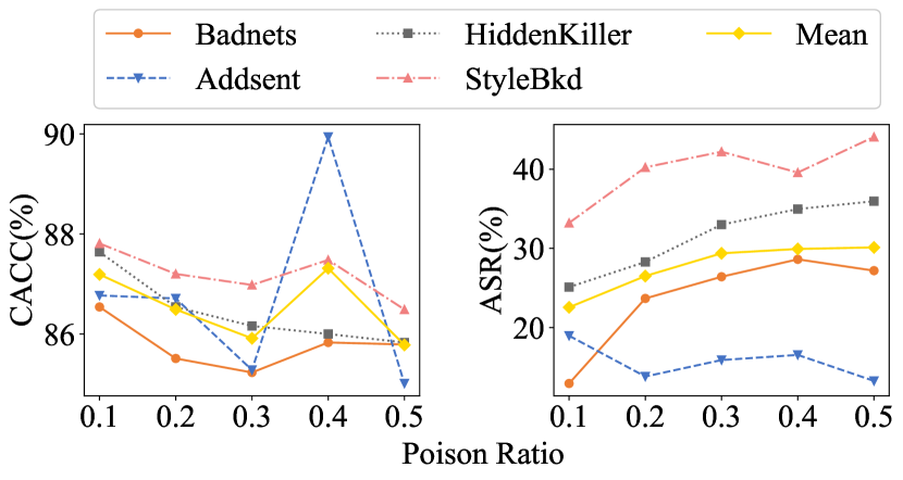
Additionally, we conduct experiments to investigate the impact of the poison ratio on backdoor mitigation performance. As shown in Figure 4, the ASR gradually rises as the poison ratio increases, yet it remains within an acceptable range for all attacks. Meanwhile, the CACC fluctuates within a small range with the increasing poison ratio. These results indicate that MuScleLoRA can maintain satisfactory backdoor mitigation performance under varying poison ratios.

5.3 Ablation Study

Dataset	Method	Strategies			Badnets		Addsent		HiddenKiller		StyleBkd
		MS	LR	GA	CACC$\uparrow$	ASR$\downarrow$	CACC$\uparrow$	ASR$\downarrow$	CACC$\uparrow$	ASR$\downarrow$	CACC$\uparrow$	ASR$\downarrow$
SST-2	Vanilla	$\times$	$\times$	$\times$	91.27	94.63	90.99	99.89	91.10	93.53	91.71	77.19
	MuscleLoRA	$\checkmark$	$\checkmark$	$\checkmark$	86.54	12.94	86.77	18.97	87.64	25.11	87.81	33.22
	w/o MS, GA	$\times$	$\checkmark$	$\times$	89.07	65.57	88.96	96.16	88.58	52.96	88.91	57.24
	w/o MS, LR	$\times$	$\times$	$\checkmark$	91.37	90.13	90.06	100	90.39	86.40	91.21	70.61
	w/o GA	$\checkmark$	$\checkmark$	$\times$	87.64	42.76	87.75	75.22	86.88	37.39	87.26	54.17
	w/o MS	$\times$	$\checkmark$	$\checkmark$	83.20	24.89	82.81	20.06	81.77	38.92	80.62	45.83
AG	Vanilla	$\times$	$\times$	$\times$	92.80	51.25	92.75	100	92.78	99.47	92.06	87.59
	MuscleLoRA	$\checkmark$	$\checkmark$	$\checkmark$	87.74	2.35	87.72	3.90	86.05	17.02	87.97	2.67
	w/o MS, GA	$\times$	$\checkmark$	$\times$	89.59	3.28	89.05	100	89.01	98.16	88.39	77.76
	w/o MS, LR	$\times$	$\times$	$\checkmark$	92.24	63.13	92.65	100	93.10	99.98	93.01	92.19
	w/o GA	$\checkmark$	$\checkmark$	$\times$	89.92	2.63	89.55	99.94	89.55	97.54	89.13	71.78
	w/o MS	$\times$	$\checkmark$	$\checkmark$	84.32	2.39	84.85	4.07	84.26	8.18	86.38	2.79

Table 3: The results of ablation experiments when adopting $\text{BERT}_{\text{Base}}$ as the target LM on SST-2 and Agnews. Bold values indicate optimal ASRs and underlined values indicate suboptimal ASRs.

We examine the contributions of three strategies in MuScleLoRA to the results, i.e., multiple radial scalings (MS), low-rank adaptation (LR), and gradient alignment (GA). The ablation results on $\text{BERT}_{\text{Base}}$ shown in Table 3 indicate that when only deploying low-rank adaptation, i.e., the LoRA baseline, the ASR drops nearly 20% on SST-2 but nearly remains unchanged on Agnews. Similarly, utilizing solely gradient alignment yields nearly minimal changes in ASR across both datasets. This suggests that aligning the gradient to clean auxiliary data, without additional defense strategies, fails to mitigate the impact of the poisoned gradient.

Compared to employing a single strategy, integrating multiple radial scalings with low-rank adaptation results in a lower ASR than the LoRA baseline, potentially achieving suboptimal ASR. Additionally, utilizing gradient alignment to low-rank adaptation can reduce ASR for several attacks to suboptimal levels, while achieving the optimal ASR on AGnews. Yet, without multiple radial scalings to enhance learning by downscaling clean mapping, CACC drops to an unacceptable level in this scenario. Consequently, MuScleLoRA combines three strategies, generally achieving the lowest ASR while maintaining acceptable CACC. More ablations are provided in Appendix C.2.

5.4 Fourier Analyses

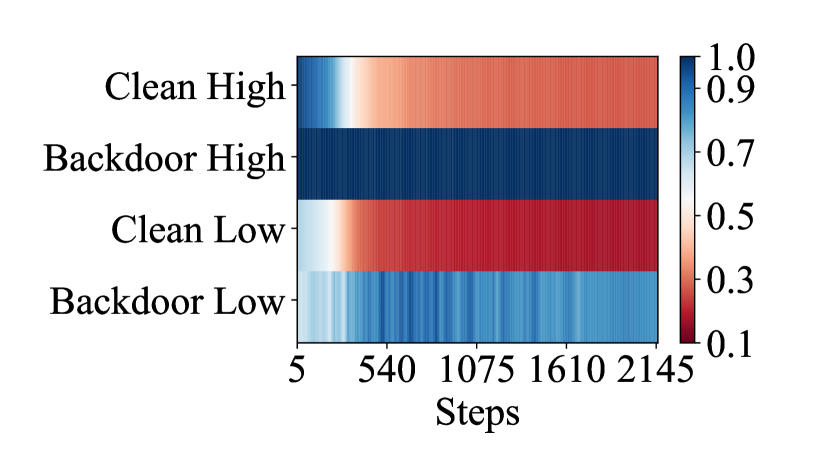
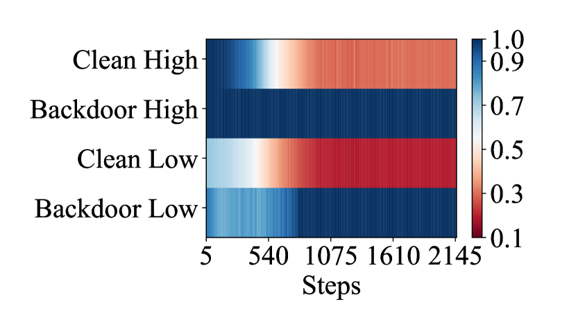
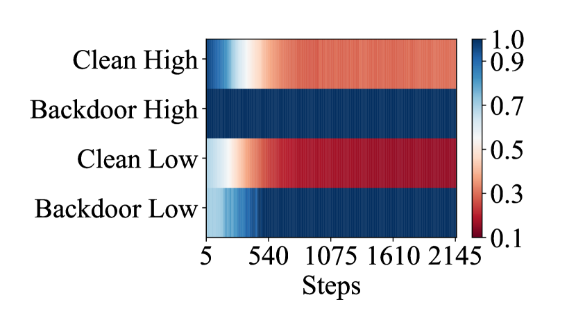
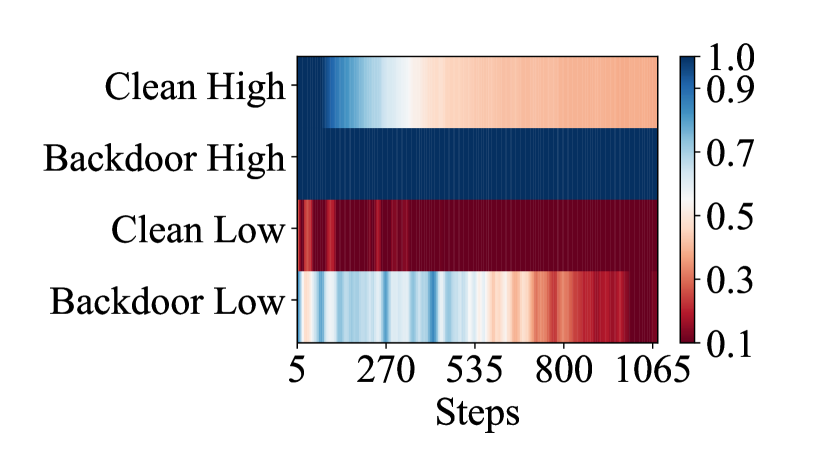
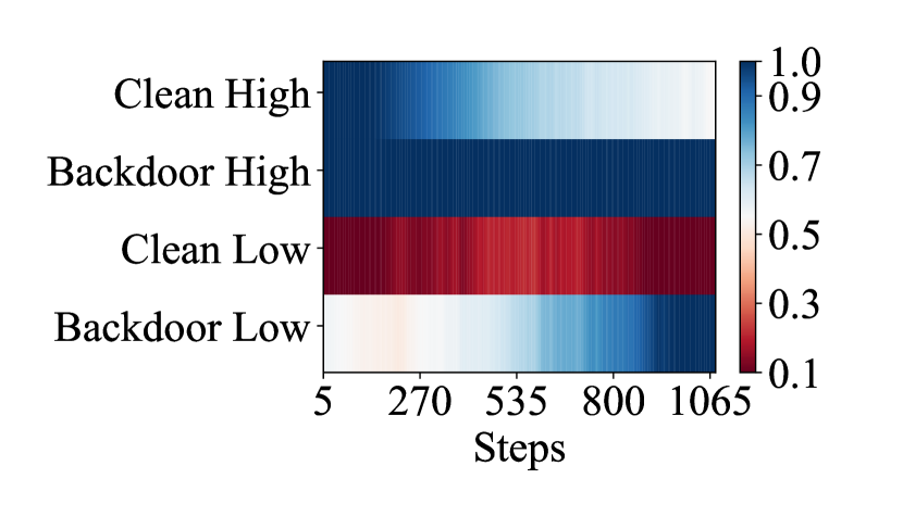
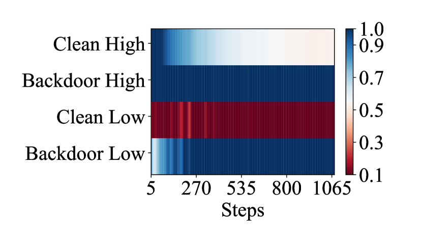
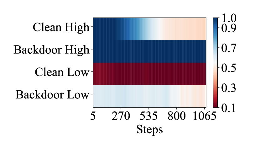
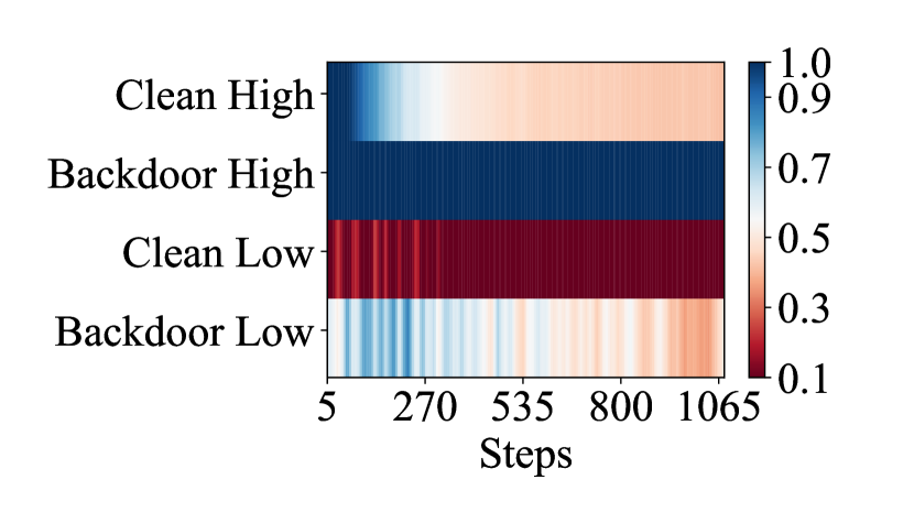
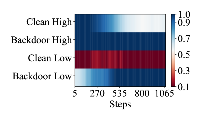
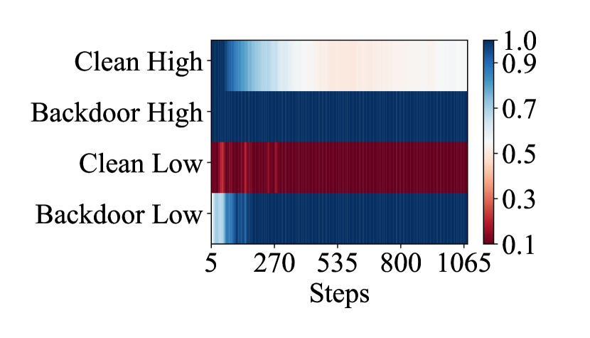
To explain the mechanisms of MuScleLoRA in the frequency space, Fourier analyses are conducted on MuScleLoRA and its ablation methods. The results on $\text{BERT}_{\text{Base}}$ are shown in Figure 5. More results on other LMs are provided in Appendix C.3.

(a) w/o MS, GA

(b) w/o GA

(c) w/o MS

(d) MuScleLoRA

Figure 5: Relative errors of MuScleLoRA and its ablation methods when adopting $\text{BERT}_{\text{Base}}$ as the target LM on Badnets poisoned SST-2 during training.

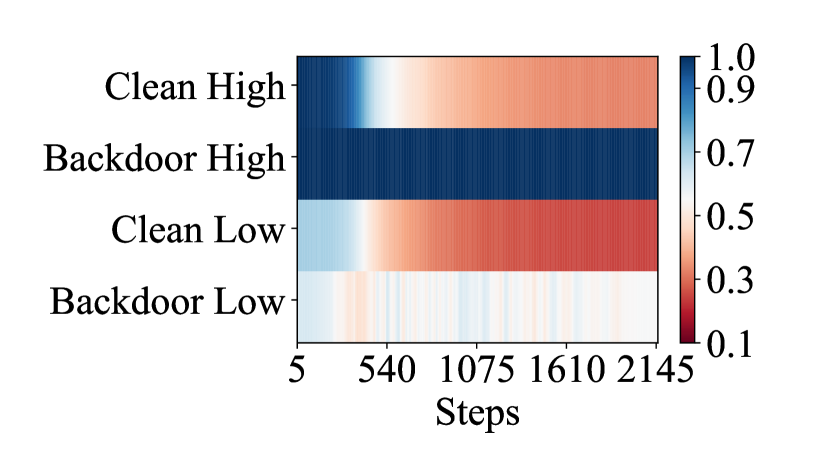
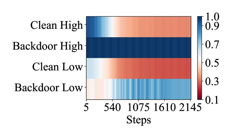
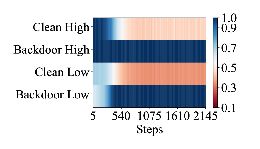
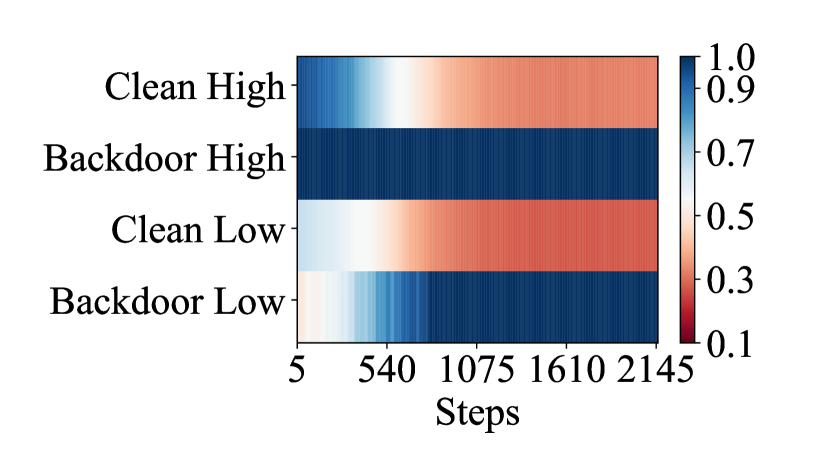
Compared to no defense deployment shown in Figure 2(a), MuScleLoRA and its ablation methods impede the convergence of low-frequency-dominated backdoor mapping. However, as shown in Figure 5(b), despite multiple radial scalings expediting the convergence of clean mapping and further hindering the learning process of backdoor mapping compared to LoRA baseline, backdoor mapping still exhibits partial convergence. These phenomena indicate that straightforward model capacity reduction with PET methods fails to effectively defend against complex triggers. Conversely, as shown in Figure 5(c), when aligning gradients to clean auxiliary data in the absence of radial scalings, the convergence of backdoor mapping is effectively hindered, but at the expense of underfitting clean mapping. Therefore, as shown in Figure 5(d), MuScleLoRA integrates multiple scalings to enhance the learning of clean mapping, facilitating the balance between backdoor mitigation and satisfactory performance in downstream tasks.

5.5 Performance on Llama2

Since PET emerges as a novel fine-tuning paradigm for LLMs, we extend MuScleLoRA to $\text{Llama2}_{\text{7B}}$ for classification, which focuses specifically on the vertical sentiment analysis task on SST-2. The backdoor mitigation performance on $\text{Llama2}_{\text{7B}}$ is presented in Table 4. Notably, MuScleLoRA consistently achieves the lowest ASR for three attacks. Conversely, due to the significant capacity increase in $\text{Llama2}_{\text{7B}}$, PET baselines and end-to-end baselines struggle to effectively counter these complex triggers. Additionally, given the extensive model capacity of $\text{Llama2}_{\text{7B}}$, the decrease in CACC attributed to low-rank adaptation and gradient alignment can be deemed negligible. These findings indicate the potential for deploying MuScleLoRA in instruction-based fine-tuning of LLMs (Zhang et al., 2023a).

Defense	Addsent		HiddenKiller		StyleBkd
	CACC$\uparrow$	ASR$\downarrow$	CACC$\uparrow$	ASR$\downarrow$	CACC$\uparrow$	ASR$\downarrow$
Vanilla	97.42	100	96.05	96.05	96.43	98.58
LoRA	95.39	93.53	94.45	78.07	95.61	93.86
Prefix	93.52	56.91	92.42	60.20	93.52	96.05
ONION	91.65	85.74	86.27	96.05	88.91	97.80
STRIP	95.66	97.48	91.71	94.29	95.44	95.18
MuscleLoRA	94.07	13.92	94.62	26.86	94.73	39.03

Table 4: Backdoor mitigation performance of MuScleLoRA, PET baselines, and post-training end-to-end baselines when adopting $\text{Llama2}_{\text{7B}}$ on SST-2.

6 Conclusions

In this paper, we conduct Fourier analyses to investigate the mechanisms of backdoor learning, revealing a notable inclination towards lower frequencies in backdoor mapping compared to clean mapping. Inspired by this observation, we proposed MuScleLoRA, a general backdoor defense method. By downscaling in the frequency space, MuScleLoRA encourages LMs to prioritize the learning of relatively high-frequency clean mapping, consequently mitigating backdoor learning. Experimental results show the efficacy of MuScleLoRA in defending against diverse backdoor attacks. Notably, MuScleLoRA exhibits generality across various backbone LMs, including BERT, RoBERTa, and Llama2.

7 Limitations

Our approach has limitations in two main aspects. First, our method only focuses on the scenario where the defender trains the target LM on the attacker-released poisoned dataset. Other scenarios, such as fine-tuning the poisoned LM on the clean dataset or, more rigorously, fine-tuning the poisoned LM on the poisoned dataset, need further exploration. Second, the scaling factor vector $S$ is relative to the model structure and capacity, requiring pre-training to determine the suitable $S$.

8 Ethics Statement

We propose a general backdoor defense method named MuScleLoRA, designed for scenarios where the defender trains the target LM on the attacker-released poisoned dataset. As all experiments are conducted on publicly available datasets and publicly available models, we believe that our proposed defense method poses no potential ethical risk.

Our created artifacts are intended to provide researchers or users with a tool for acquiring clean language models from backdoor poisoned datasets. All use of existing artifacts is consistent with their intended use in this paper.

Appendix A Filtering-based Fourier Transformation

In this section, we provide the detailed processes of filtering-based Fourier transformation used to extract the low-frequency and high-frequency parts of the target-LM-fitted and ground-truth mappings.

We denote the training dataset of the target LM as $\{x_{i},t_{i}\}_{i=1}^{N}=(X,T)$, where $x_{i}=\{x_{i}^{1},\cdots,x_{i}^{L}\}$, $L$, $t_{i}\in\mathbb{R}^{C}$, $X=\{x_{1};\cdots;x_{N}\}\in\mathbb{R}^{N\times L}$, and $T=\{t_{1};\cdots;t_{N}\}\in\mathbb{R}^{N\times C}$ denote the input ids of the input text with length $L$, the ground-truth one-hot label, the input matrix, and the label matrix, respectively. Notably, LMs often convert discrete input ids into continuous embeddings, i.e., $e=\mathcal{E}(x),e\in\mathbb{R}^{L\times d}$, where $\mathcal{E}$ denotes the embedding layer of the target LM and $d$ denotes the embedding dimension. Besides, embedding updates during training typically exhibit small magnitudes. For simplicity, we assume that the embedding of each input id remains unchanged throughout training. Consequently, the mapping fitted by the target LM can be illustrated as Equation 9, where $y\in\mathbb{R}^{C}$, $Y=\{y_{1};\cdots;y_{N}\}\in\mathbb{R}^{N\times C}$, and $E=\{e_{1};\cdots;e_{N}\}\in\mathbb{R}^{N\times L\times d}$ denote the output logits, the matrix of output logits, and the tensor of input embeddings, respectively.

$$\mathcal{F}:\mathbb{R}^{L\times d} \to\mathbb{R}^{C},$$ (9)

$$\mathcal{F}(e) =y,$$

$$\mathcal{F}(E) =Y.$$

Similarly, the ground-truth mapping utilizing the same embedding layer is illustrated as Equation 10.

$$\mathcal{T} :\mathbb{R}^{L\times d}\to\mathbb{R}^{C},$$ (10)

$$\mathcal{T} (e)=t,$$

$$\mathcal{T} (E)=T.$$

Practically, when $C>1$, $\mathcal{F}$ represents the high-dimensional mapping. In such scenarios, employing the high-dimensional discrete Fourier transformation incurs significant computational overhead, posing challenges for real dataset analysis. Therefore, we opt for a pragmatic approach by partitioning the frequency space into two segments, i.e., the low-frequency part with $|\xi|\leq\xi_{0}$ and the high-frequency part with $|\xi|>\xi_{0}$, to decompose the mapping into the low-frequency part and high-frequency part, respectively. Specifically, we denote the Fourier transformation of $\mathcal{F}$ as $\hat{\mathcal{F}}$ and then decompose $\hat{\mathcal{F}}$ by the indicator $\mathcal{I}(|\xi|\leq\xi_{0})$ that indicate the low-frequency part in the frequency space, which is illustrated as Equation 11.

$$\hat{\mathcal{F}}^{\text{low}} =\hat{\mathcal{F}}\cdot\mathcal{I}(|\xi|\leq\xi_{0}),$$ (11)

$$\hat{\mathcal{F}}^{\text{high}} =\hat{\mathcal{F}}-\hat{\mathcal{F}}^{\text{low}}.$$

To further alleviate the computational cost of the high-dimensional indicator, we alternatively apply Gaussian filter $\hat{G}^{\frac{1}{\delta}}(\xi)$ to approximate the indicator $\mathcal{I}(|\xi|\leq\xi_{0})$, i.e., $\hat{\mathcal{F}}^{\text{low}}\approx\hat{\mathcal{F}}\cdot\hat{G}^{\frac{1}{\delta}}$, where $\frac{1}{\delta}$ denotes the variance of the Gaussian filter in the frequency space. Consequently, in the corresponding physical space, the low-frequency part $y^{\text{low},\delta}_{i}$ and high-frequency part $y^{\text{high},\delta}_{i}$ of the output logits $y_{i}$ for the entire dataset are obtained through Gaussian convolution, as illustrated in Equation 12. Here, $G^{\delta}(e_{i}^{\prime}-e_{j}^{\prime})=\mathrm{e}^{\frac{-\|e_{i}^{\prime}-e_{j}^{\prime}\|^{2}}{2\delta}}$ denotes the corresponding Gaussian filter in the physical space with variance $\delta$, $e_{i}^{\prime}\in\mathbb{R}^{Ld}$ denotes the flattened vector of the embedding $e_{i}$, $C_{i}=\sum_{j=1}^{N}G^{\delta}(e_{i}^{\prime}-e_{j}^{\prime})$ denotes the normalization factor, and $G\in\mathbb{R}^{N\times N},G_{ij}=G^{\delta}(e_{i}^{\prime}-e_{j}^{\prime})$ denotes the matrix of Gaussian filters, respectively. Practically, we set $\delta$ to 4.0 to obtain frequency components.

$$y^{\text{low},\delta}_{i} =\frac{1}{C_{i}}\sum_{j=1}^{N}y_{j}G^{\delta}(e_{i}^{\prime}-e_{j}^{\prime})$$ (12)

$$=\frac{1}{C_{i}}(GY)_{i},$$

$$y^{\text{high},\delta}_{i} =y_{i}-y^{\text{low},\delta}_{i}$$

$$=\left(Y-\frac{1}{C_{i}}(GY)\right)_{i}.$$

Same as the analysis of output logits, for ground-truth labels, we can derive their respective frequency components, i.e., $t^{\text{low},\delta}_{i}$ and $t^{\text{high},\delta}_{i}$, by Gaussian convolution, as illustrated in Equation 13.

$$t^{\text{low},\delta}_{i} =\frac{1}{C_{i}}\sum_{j=1}^{N}t_{j}G^{\delta}(e_{i}^{\prime}-e_{j}^{\prime})$$ (13)

$$=\frac{1}{C_{i}}(GT)_{i},$$

$$t^{\text{high},\delta}_{i} =t_{i}-t^{\text{low},\delta}_{i}$$

$$=\left(T-\frac{1}{C_{i}}(GT)\right)_{i}.$$

Appendix B Detailed Experiment Setup

In this section, we provide additional setup information for experiments. In Section B.1, we provide the detailed statistics of datasets. Subsequently, in Section B.2, we provide comprehensive descriptions of defense baselines. Additionally, we outline detailed trigger settings in Section B.3. Besides, Section B.4 elaborates on hyperparameter settings. Furthermore, Section B.5 provides the usage of existing artifacts.

B.1 Datasets

The statistics of datasets are presented in Table 5. Considering the excessive number of samples in Agnews, which could potentially prolong the training process, we decided to randomly extract 5,000 samples from each class in the original training dataset. Consequently, a new training dataset comprising 20,000 samples is synthesized.

Dataset	Categories	Number of Samples			Average Length
		Train	Test	Validation
SST-2	2	6,920	1,821	872	19.2
HSOL	2	5,823	2,485	2,485	13.2
Lingspam	2	2,604	582	289	695.3
Agnews	4	108,000	7,600	12,000	38.0

Table 5: Detailed statistics of datasets.

B.2 Defense Baselines

PET baselines.

PET baselines reduce model capacity by freezing the original weights of the LM and inserting tunable PET modules with a small number of parameters, constraining the model to focus on clean tasks (Zhu et al., 2022). LoRA (Hu et al., 2022) inserts parallel low-rank decompositions as the tunable module. Adapter (Houlsby et al., 2019) inserts a sequential linear layer as the tunable module. Prefix-Tuning (Li and Liang, 2021) inserts a sequence of continuous task-specific vectors as the tunable module.

ONION.

Based on the observation that inserting trigger words into original text results in a notable increase in perplexity, ONION (Qi et al., 2021a) utilizes GPT-2 to quantify the contribution of each word in the original text to the perplexity and detect high-contributing words as the trigger words.

STRIP.

Based on the observation that clean text is more sensitive to perturbations than poisoned text, STRIP (Gao et al., 2021) employs random word replacement to perturb input text, subsequently identifying poisoned text by analyzing discrepancy in the entropy of output logits.

RAP.

Similar to STRIP, RAP (Yang et al., 2021) discerns poisoned input texts based on their sensitivity to perturbations. RAP reconfigures the embedding layer to incorporate a robust-aware perturbation to be introduced into input texts, which significantly alters the logits of clean texts while minimally affecting poisoned samples.

BKI.

Similar to ONION, BKI (Chen and Dai, 2021) quantifies the contribution of each word in the original text of the training dataset to the output logits to detect high-contributing words as the trigger words.

CUBE.

Based on the observation that poisoned samples frequently manifest as outliers in the feature space, CUBE (Cui et al., 2022) clusters samples in the training dataset to identify outliers as the poisoned samples.

B.3 Trigger Settings

For Badnets, following the settings of Kurita et al. (2020), we insert 4 rare words, i.e., cf, mn, bb, and tq, into random positions within the original text. For Addsent, following the settings of Dai et al. (2019), we insert a predefined sentence, i.e., I watch this 3D movie, into a random position within the original text. For HiddenKiller, following the settings of Qi et al. (2021c), we adopt ( ROOT ( S ( SBAR ) ( , ) ( NP ) ( VP ) ( . ) ) ) EOP as the trigger syntax. We then paraphrase the entire original text into trigger syntax for the sentence-level datasets: SST-2, HSOL, and Agnews. Additionally, for the paragraph-level dataset Lingspam, each sentence in the original text is paraphrased into trigger syntax. For StyleBkd, following the settings of Qi et al. (2021b), we choose bible text style as the trigger style. Similar to HiddenKiller, we paraphrase the entire original text into trigger style for the sentence-level datasets: SST-2, HSOL, and Agnews, while every sentence in the original text is paraphrased into trigger style for the paragraph-level dataset Lingspam.

B.4 Hyperparameters

Notably, compared to the meticulous hyperparameter design by Zhu et al. (2022) tailored for different attacks, we unify hyperparameters against diverse attacks for each specific LM. Specifically, following the observation that reducing the training epochs can mitigate backdoor learning (Zhu et al., 2022), we set training epochs to 10 for BERT and RoBERTa, and 5 for $\text{Llama2}_{\text{7B}}$. Similarly, we set learning rate to $2\times 10^{-5}$ for BERT and RoBERTa, and $10^{-5}$ for Llama2. Additionally, considering the extensive model capability of $\text{Llama2}_{\text{7B}}$, the number of clean auxiliary data for $\text{Llama2}_{\text{7B}}$ is set to 128 whereas it is set to 96 for BERT and RoBERTa. Furthermore, $\mu_{\max}$ is configured to 0 for $\text{Llama2}_{\text{7B}}$ and 0.1 for BERT and RoBERTa. The batch size is defined as 16 for $\text{Llama2}_{\text{7B}}$ and 32 for BERT and RoBERTa. For PET baselines, the bottleneck dimensions are uniformly set to 8 for BERT and RoBERTa and 2 for $\text{Llama2}_{\text{7B}}$. Finally, detailed settings of the scaling factor vector $S$ are presented in Table 6, and the bandwidth $r$ of each $A_{i}$ in radial scalings is specified as only 1. All experiments are conducted on NVIDIA GeForce RTX 3090 with 24GB memory.

Model	$S$
$\text{BERT}_{\text{Base}}$	$[1,4,8,12,16,20,24,28,32]$
$\text{BERT}_{\text{Large}}$	$[1,2,3,4,5,6,7,8,9]$
$\text{RoBERTa}_{\text{Base}}$	$[1,2,4,6,8,10,12,14,16]$
$\text{RoBERTa}_{\text{Large}}$	$[1,2,3,4,5,6,7,8,9]$
$\text{Llama2}_{\text{7B}}$	$[1,2,3,4]$

Table 6: Detailed settings of scaling factor vector $S$.

B.5 Usage of Existing Artifacts

For conducting backdoor attacks and end-to-end defense baselines, we employ OpenBackdoor (Cui et al., 2022), an open-source framework for textual backdoor learning. The detailed process of MuScleLoRA is implemented within the framework of PyTorch (Paszke et al., 2019), an open-source library for deploying deep learning. For implementing PET algorithms, we utilize Huggingface-PEFT (Mangrulkar et al., 2022), an open-source library for HuggingFace-transformers-based PET methods of LMs, and Opendelta (Hu et al., 2023), another open-source library dedicated to PET methods of LMs. For LMs, we adopt BERT, RoBERTa, and $\text{Llama2}_{\text{7B}}$ from Huggingface transformers. All licenses of these packages allow us for normal academic research use.

Appendix C Additional Experimental Results and Analyses

In this section, we provide additional experimental results and analyses. Section C.1 provides the backdoor mitigation performance on $\text{BERT}_{\text{Large}}$, $\text{RoBERTa}_{\text{Base}}$, and $\text{RoBERTa}_{\text{Large}}$. Subsequently, we conduct the ablation studies on the three strategies in MuScleLoRA when adopting $\text{BERT}_{\text{Large}}$, $\text{RoBERTa}_{\text{Base}}$, or $\text{RoBERTa}_{\text{Large}}$ as the target LM in Section C.2, perform Fourier analyses on $\text{BERT}_{\text{Large}}$ and $\text{Llama2}_{\text{7B}}$ to explain the mechanisms of MuScleLoRA in Section C.3, and analyze the sensitivity on hyperparameters in Section C.4.

Dataset	Model	Defense	Badnets		Addsent		HiddenKiller		StyleBkd
			CACC$\uparrow$	ASR$\downarrow$	CACC$\uparrow$	ASR$\downarrow$	CACC$\uparrow$	ASR$\downarrow$	CACC$\uparrow$	ASR$\downarrow$
SST-2	$\text{BERT}_{\text{Large}}$	Vanilla	92.91	93.64	92.97	100	92.64	90.24	93.30	78.51
		LoRA	91.98	31.14	91.27	84.87	91.54	42.21	90.50	66.67
		Adapter	89.73	40.57	88.85	70.17	89.51	42.98	89.07	64.14
		Prefix	92.42	37.06	92.04	99.56	92.59	67.98	91.93	57.90
		MuscleLoRA	91.21	14.80	90.71	27.30	90.99	17.54	89.62	21.16
	$\text{RoBERTa}_{\text{Base}}$	Vanilla	94.39	95.61	94.17	99.89	93.13	93.86	94.67	99.34
		LoRA	92.09	26.54	91.87	63.05	90.99	38.60	91.54	67.33
		Adapter	91.43	57.46	88.69	62.39	91.49	33.77	90.45	69.96
		Prefix	91.98	85.19	91.98	100	90.94	62.94	92.36	94.96
		MuscleLoRA	88.08	13.26	88.91	21.16	89.07	20.28	88.41	20.61
	$\text{RoBERTa}_{\text{Large}}$	Vanilla	94.29	100	95.44	100	93.52	90.24	94.45	99.12
		LoRA	95.55	11.73	94.95	92.21	95.94	57.24	95.39	73.03
		Adapter	70.01	99.78	58.81	35.52	58.10	52.19	62.55	96.05
		Prefix	94.89	76.54	94.56	78.73	93.96	62.50	94.62	89.14
		MuscleLoRA	93.30	5.81	93.19	14.47	92.59	10.96	92.48	12.39
AG	$\text{BERT}_{\text{Large}}$	Vanilla	93.71	63.86	93.56	100	93.53	99.32	93.18	88.21
		LoRA	90.67	1.68	90.55	99.81	90.32	97.21	90.21	82.99
		Adapter	90.16	3.68	89.45	66.53	89.74	91.00	88.97	36.72
		Prefix	92.39	54.81	92.54	100	91.75	99.10	91.76	82.99
		MuscleLoRA	89.58	1.67	89.10	1.70	87.33	28.04	88.97	12.15
	$\text{RoBERTa}_{\text{Base}}$	Vanilla	93.29	86.19	93.68	100	93.32	99.98	93.56	91.56
		LoRA	90.54	1.86	90.22	99.96	90.53	99.93	89.93	81.28
		Adapter	90.60	3.40	89.85	99.98	90.39	99.70	88.96	78.77
		Prefix	91.05	39.51	91.12	99.95	90.87	99.96	90.33	84.63
		MuscleLoRA	86.89	1.42	86.30	1.35	87.01	19.46	86.78	5.70
	$\text{RoBERTa}_{\text{Large}}$	Vanilla	93.79	96.42	93.14	100	93.66	100	93.59	94.40
		LoRA	92.14	2.21	92.24	99.96	91.96	99.90	91.63	88.44
		Adapter	91.10	2.39	91.10	99.95	90.83	99.23	90.75	72.75
		Prefix	92.34	18.60	92.18	99.96	92.21	99.98	91.82	91.12
		MuscleLoRA	90.21	1.85	90.10	4.26	89.64	7.34	90.05	2.30

Table 7: Backdoor mitigation performance of MuScleLoRA and PET baselines when adopting $\text{BERT}_{\text{Large}}$, $\text{RoBERTa}_{\text{Base}}$, or $\text{RoBERTa}_{\text{Large}}$ as the target LM on SST-2 and Agnews. Bold values indicate optimal ASRs.

Model	Method	Strategies			Badnets		Addsent		HiddenKiller		StyleBkd
		MS	LR	GA	CACC$\uparrow$	ASR$\downarrow$	CACC$\uparrow$	ASR$\downarrow$	CACC$\uparrow$	ASR$\downarrow$	CACC$\uparrow$	ASR$\downarrow$
$\text{BERT}_{\text{Large}}$	Vanilla	$\times$	$\times$	$\times$	92.91	93.64	92.97	100	92.64	90.24	93.30	78.51
	MuscleLoRA	$\checkmark$	$\checkmark$	$\checkmark$	91.21	14.80	90.72	27.30	90.99	17.54	89.62	21.16
	w/o MS, GA	$\times$	$\checkmark$	$\times$	91.98	31.14	91.27	84.87	91.54	42.21	90.50	66.67
	w/o MS, LR	$\times$	$\times$	$\checkmark$	93.68	89.91	92.53	100	91.98	86.62	92.58	74.67
	w/o GA	$\checkmark$	$\checkmark$	$\times$	91.54	29.71	90.28	75.22	90.94	44.71	89.62	54.47
	w/o MS	$\times$	$\checkmark$	$\checkmark$	86.54	29.82	86.16	36.84	87.37	27.85	85.94	28.29
$\text{RoBERTa}_{\text{Base}}$	Vanilla	$\times$	$\times$	$\times$	94.39	95.61	94.17	99.89	93.13	93.86	94.67	99.34
	MuscleLoRA	$\checkmark$	$\checkmark$	$\checkmark$	88.08	13.26	88.91	21.16	89.07	20.28	88.41	20.61
	w/o MS, GA	$\times$	$\checkmark$	$\times$	92.09	26.54	9187	63.05	90.99	38.60	91.54	67.33
	w/o MS, LR	$\times$	$\times$	$\checkmark$	92.86	94.30	93.46	100	90.06	87.61	94.12	96.71
	w/o GA	$\checkmark$	$\checkmark$	$\times$	93.30	24.45	92.53	65.57	92.31	48.68	92.81	40.46
	w/o MS	$\times$	$\checkmark$	$\checkmark$	80.72	25.22	80.45	22.92	82.87	22.81	84.57	23.13
$\text{RoBERTa}_{\text{Large}}$	Vanilla	$\times$	$\times$	$\times$	94.29	100	95.44	100	93.52	90.24	94.45	99.12
	MuscleLoRA	$\checkmark$	$\checkmark$	$\checkmark$	93.30	5.81	93.19	14.47	92.59	10.96	92.48	12.39
	w/o MS, GA	$\times$	$\checkmark$	$\times$	95.55	11.73	94.95	92.21	95.94	57.24	95.39	73.03
	w/o MS, LR	$\times$	$\times$	$\checkmark$	94.95	67.21	95.44	100	95.28	90.24	95.39	92.21
	w/o GA	$\checkmark$	$\checkmark$	$\times$	94.84	13.05	94.40	70.83	95.28	44.74	95.72	71.49
	w/o MS	$\times$	$\checkmark$	$\checkmark$	89.79	10.31	90.39	18.75	91.05	16.45	91.43	16.67

Table 8: The results of ablation experiments on SST-2 when adopting $\text{BERT}_{\text{Large}}$, $\text{RoBERTa}_{\text{Base}}$, or $\text{RoBERTa}_{\text{Large}}$ as the respective target LM. Bold values indicate optimal ASRs and underlined values indicate suboptimal ASRs.

C.1 Performance of Backdoor Mitigation

We further evaluate the backdoor mitigation performance on $\text{BERT}_{\text{Large}}$, $\text{RoBERTa}_{\text{Base}}$, and $\text{RoBERTa}_{\text{Large}}$. As presented in Table 7, similar to the results presented in Table 1, although PET baselines manage to reduce the ASR for Badnets to a relatively low level, they still encounter challenges in effectively defending against other complex triggers. Conversely, MuScleLoRA consistently reduces the ASR to the lowest level, surpassing the performance of the three PET baselines significantly. Moreover, in comparison to the about 4-5% decrease in CACC when implementing MuScleLoRA on $\text{BERT}_{\text{Base}}$, the decrease in CACC for $\text{BERT}_{\text{Large}}$ and $\text{RoBERTa}_{\text{Large}}$ is negligible. This suggests that a larger model capacity can alleviate the reduction in CACC while preserving low ASR when deploying MuScleLoRA.

Also, we evaluate the backdoor mitigation performance of MuScleLoRA with end-to-end defense baselines on $\text{BERT}_{\text{Large}}$. As presented in Table 9, MuScleLoRA achieves the optimal ASRs, surpassing all end-to-end baselines.

Defense	Addsent		HiddenKiller		StyleBkd
	CACC$\uparrow$	ASR$\downarrow$	CACC$\uparrow$	ASR$\downarrow$	CACC$\uparrow$	ASR$\downarrow$
Vanilla	92.97	100	92.64	90.24	93.30	78.51
ONION	88.14	93.09	86.27	96.16	87.48	79.56
BKI	92.20	100	91.16	92.65	92.31	81.58
CUBE	93.24	100	92.53	21.93	91.65	31.47
STRIP	72.43	60.64	92.09	91.67	89.17	75.76
RAP	92.04	100	90.94	92.98	87.66	69.08
MuScleLoRA	90.71	27.30	90.99	17.54	89.62	21.16

Table 9: Backdoor mitigation performance of MuScleLoRA and end-to-end baselines when adopting $\text{BERT}_{\text{Large}}$ as the target LM on SST-2. Bold values indicate optimal ASRs.

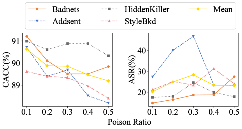
Furthermore, experiments are performed to explore the impact of poison ratio on ASR and CACC when adopting $\text{BERT}_{\text{Large}}$ as the target LM. As shown in Figure 6, as the poison ratio increases, CACC exhibits a slight decrease, while ASR fluctuates within an acceptable range.

Figure 6: CACC and ASR of MuScleLoRA when adopting $\text{BERT}_{\text{Large}}$ as the target LM on poisoned SST-2 under diverse poison ratios.

C.2 Ablation Study

Additionally, we examine the contribution of three strategies in MuScleLoRA to the performance on SST-2 when adopting $\text{BERT}_{\text{Large}}$, $\text{RoBERTa}_{\text{Base}}$, or $\text{RoBERTa}_{\text{Large}}$ as the target LM, respectively. The results of the ablation analyses are presented in Table 8. Similar to the ablation of $\text{BERT}_{\text{Base}}$, solely employing low-rank adaptation or gradient alignment encounters challenges in effectively defending against diverse backdoor attacks. Moreover, the absence of radial scalings leads to a significant drop in CACC. Optimal performance is achieved only when all three strategies are combined.

C.3 Fourier analyses

We further conduct Fourier analyses on MuScleLoRA and its ablation methods on $\text{BERT}_{\text{Large}}$ and $\text{Llama2}_{\text{7B}}$. The results are shown in Figure 11, Figure 12, and Figure 13, respectively. Compared to the relatively underfitting of $\text{BERT}_{\text{Base}}$, larger-scale $\text{BERT}_{\text{Large}}$ and $\text{Llama2}_{\text{7B}}$ obtain better convergence in clean mapping. Furthermore, given that deeper models tend to exhibit stronger low-frequency bias (Xu and Zhou, 2021), $\text{Llama2}_{\text{7B}}$ exhibits rapid convergence in the low-frequency part.

Moreover, as shown in Figure 11(b), Figure 11(d), Figure 12(b), Figure 12(d), Figure 13(b), and Figure 13(d), multiple radial scalings expedite the convergence of clean mapping significantly. Furthermore, as shown in Figure 12(b) and Figure 13(b), only adopting multiple radial scalings with low-rank adaptation hinders the early-stage convergence of backdoor mapping.

However, due to the excessive model capacity of $\text{Llama2}_{\text{7B}}$, the backdoor mapping demonstrates rapid convergence in the later stages of training. This observation suggests that straightforward model capacity reduction with PET methods is ineffective in defending against complex triggers, particularly on LLMs.

C.4 Hyperparameter Sensitivity Analyses

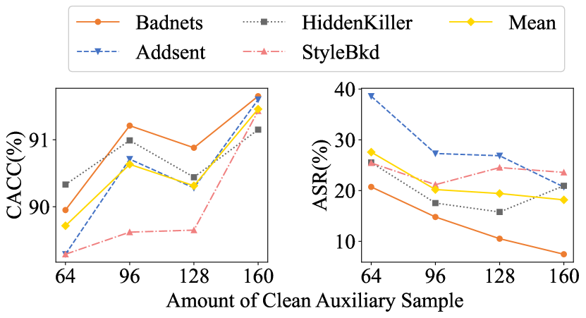
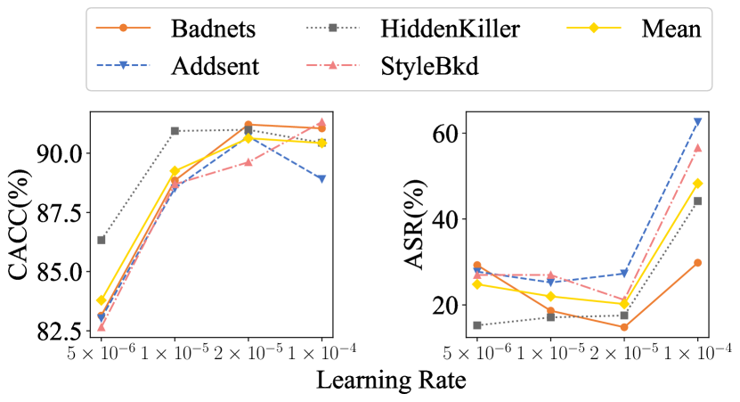
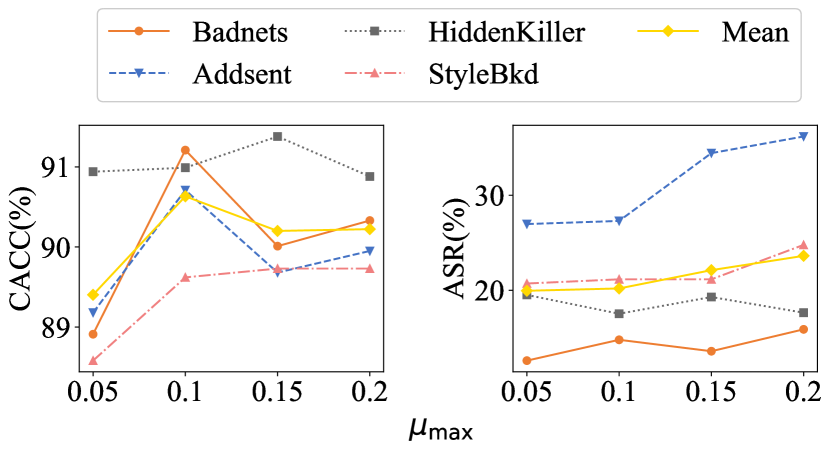
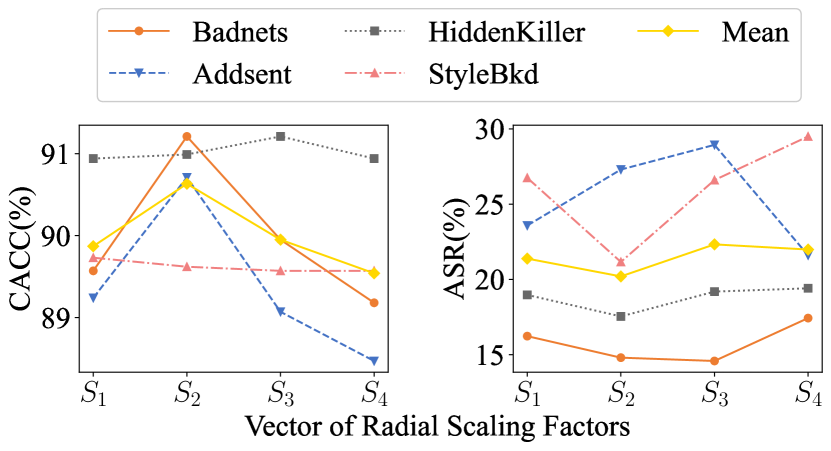
We conduct experiments to investigate the impact of different hyperparameters of MuScleLoRA on $\text{BERT}_{\text{Large}}$, including the number of clean auxiliary samples, learning rate, $\mu_{\max}$, and the vector of radial scaling factors. The results are shown in Figure 7, Figure 8, Figure 9, and Figure 10, respectively. Detailed notation for the vector of radial scaling factors is presented in Table 10.

Figure 7 illustrates that increasing the number of clean auxiliary samples yields higher CACC and lower ASR. Figure 8 demonstrates that a small learning rate induces underfitting in clean tasks, whereas a large one results in high ASR. Moderate learning rates enable a tradeoff between CACC and ASR.Figure 9 reveals that a small $\mu_{\max}$, indicating a lower proportion of the original gradient accepted, results in underfitting in clean tasks, while a large $\mu_{\max}$ can lead to low defense performance. Figure 10 illustrates that altering the vector of radial scaling factors causes fluctuations in both CACC and ASR. Therefore, selecting the appropriate vector of radial scaling factors is essential to achieve optimal backdoor mitigation performance.

Notation	$S$
$S_{1}$	$[1,1.5,2,2.5,3,3.5,4,4.5,5]$
$S_{2}$	$[1,2,3,4,5,6,7,8,9]$
$S_{3}$	$[1,2,4,6,8,10,12,14,16]$
$S_{4}$	$[1,4,8,12,16,20,24,28,32]$

Table 10: Detailed notation for scaling factor vector $S$ when adopting $\text{BERT}_{\text{Large}}$ as the target LM.

Figure 7: CACC and ASR of MuScleLoRA when adopting $\text{BERT}_{\text{Large}}$ as the target LM on poisoned SST-2 under diverse amounts of clean auxiliary samples.

Figure 8: CACC and ASR of MuScleLoRA when adopting $\text{BERT}_{\text{Large}}$ as the target LM on poisoned SST-2 under diverse learning rates.

Figure 9: CACC and ASR of MuScleLoRA when adopting $\text{BERT}_{\text{Large}}$ as the target LM on poisoned SST-2 under diverse $\mu_{\max}$.

Figure 10: CACC and ASR of MuScleLoRA when adopting $\text{BERT}_{\text{Large}}$ as the target LM on poisoned SST-2 dataset under diverse vectors of radial scaling factors.

(a) w/o MS, GA

(b) w/o GA

(c) w/o MS

(d) MuScleLoRA

Figure 11: Relative errors of MuScleLoRA and its ablation methods when adopting $\text{BERT}_{\text{Large}}$ as the target LM on Badnets poisoned SST-2 during training.

(a) w/o MS, GA

(b) w/o GA

(c) w/o MS

(d) MuScleLoRA

Figure 12: Relative errors of MuScleLoRA and its ablation methods when adopting $\text{Llama2}_{\text{7B}}$ as the target LM on Addsent poisoned SST-2 during training.

(a) w/o MS, GA

(b) w/o GA

(c) w/o MS

(d) MuScleLoRA

Figure 13: Relative errors of MuScleLoRA and its ablation methods when adopting $\text{Llama2}_{\text{7B}}$ as the target LM on HiddenKiller poisoned SST-2 during training.

References

- Azizi et al. (2021) Ahmadreza Azizi, Ibrahim Asadullah Tahmid, Asim Waheed, Neal Mangaokar, Jiameng Pu, Mobin Javed, Chandan K Reddy, and Bimal Viswanath. 2021. T-miner: A generative approach to defend against trojan attacks on dnn-based text classification. In Proceedings of the 30th USENIX Security Symposium, pages 2255–2272, Online.
- Chen and Dai (2021) Chuanshuai Chen and Jiazhu Dai. 2021. Mitigating backdoor attacks in lstm-based text classification systems by backdoor keyword identification. Neurocomputing, 452:253–262.
- Chen et al. (2017) Xinyun Chen, Chang Liu, Bo Li, Kimberly Lu, and Dawn Song. 2017. Targeted backdoor attacks on deep learning systems using data poisoning. arXiv preprint arXiv:1712.05526.
- Chen et al. (2020) Zhao Chen, Jiquan Ngiam, Yanping Huang, Thang Luong, Henrik Kretzschmar, Yuning Chai, and Dragomir Anguelov. 2020. Just pick a sign: Optimizing deep multitask models with gradient sign dropout. In Advances in Neural Information Processing Systems 33: Annual Conference on Neural Information Processing Systems 2020, Online.
- Cui et al. (2022) Ganqu Cui, Lifan Yuan, Bingxiang He, Yangyi Chen, Zhiyuan Liu, and Maosong Sun. 2022. A unified evaluation of textual backdoor learning: Frameworks and benchmarks. In Advances in Neural Information Processing Systems 35: Annual Conference on Neural Information Processing Systems 2022, volume 35, pages 5009–5023, New Orleans, USA.
- Dai et al. (2019) Jiazhu Dai, Chuanshuai Chen, and Yufeng Li. 2019. A backdoor attack against lstm-based text classification systems. IEEE Access, 7:138872–138878.
- Davidson et al. (2017) Thomas Davidson, Dana Warmsley, Michael Macy, and Ingmar Weber. 2017. Automated hate speech detection and the problem of offensive language. In Proceedings of the 2017 international AAAI conference on web and social media, volume 11, pages 512–515, Montreal, Canada.
- Devlin et al. (2019) Jacob Devlin, Ming-Wei Chang, Kenton Lee, and Kristina Toutanova. 2019. Bert: Pre-training of deep bidirectional transformers for language understanding. In Proceedings of the 2019 Conference of the North American Chapter of the Association for Computational Linguistics: Human Language Technologies, pages 4171–4186, Minneapolis, USA.
- Gao et al. (2021) Yansong Gao, Yeonjae Kim, Bao Gia Doan, Zhi Zhang, Gongxuan Zhang, Surya Nepal, Damith C Ranasinghe, and Hyoungshick Kim. 2021. Design and evaluation of a multi-domain trojan detection method on deep neural networks. IEEE Transactions on Dependable and Secure Computing, 19(4):2349–2364.
- Gu et al. (2023) Naibin Gu, Peng Fu, Xiyu Liu, Zhengxiao Liu, Zheng Lin, and Weiping Wang. 2023. A gradient control method for backdoor attacks on parameter-efficient tuning. In Proceedings of the 61st Annual Meeting of the Association for Computational Linguistics (Volume 1: Long Papers), pages 3508–3520, Toronto, Canada.
- Han et al. (2016) Song Han, Huizi Mao, and William J Dally. 2016. Deep compression: Compressing deep neural networks with pruning, trained quantization and huffman coding. In Proceedings of the 4th International Conference on Learning Representations, San Juan, Puerto Rico.
- Houlsby et al. (2019) Neil Houlsby, Andrei Giurgiu, Stanislaw Jastrzebski, Bruna Morrone, Quentin De Laroussilhe, Andrea Gesmundo, Mona Attariyan, and Sylvain Gelly. 2019. Parameter-efficient transfer learning for nlp. In Proceedings of the 36th International Conference on International Conference on Machine Learning, pages 2790–2799, Long Beach, USA.
- Hu et al. (2022) Edward J Hu, Phillip Wallis, Zeyuan Allen-Zhu, Yuanzhi Li, Shean Wang, Lu Wang, Weizhu Chen, et al. 2022. Lora: Low-rank adaptation of large language models. In Proceedings of the 10th International Conference on Learning Representations, Online.
- Hu et al. (2023) Shengding Hu, Ning Ding, Weilin Zhao, Xingtai Lv, Zhen Zhang, Zhiyuan Liu, and Maosong Sun. 2023. Opendelta: A plug-and-play library for parameter-efficient adaptation of pre-trained models. In Proceedings of the 61st Annual Meeting of the Association for Computational Linguistics (Volume 3: System Demonstrations), pages 274–281, Toronto, Canada.
- Jin et al. (2022) Lesheng Jin, Zihan Wang, and Jingbo Shang. 2022. Wedef: Weakly supervised backdoor defense for text classification. In Proceedings of the 2022 Conference on Empirical Methods in Natural Language Processing, pages 11614–11626, Abu Dhabi, United Arab Emirates.
- Kurita et al. (2020) Keita Kurita, Paul Michel, and Graham Neubig. 2020. Weight poisoning attacks on pretrained models. In Proceedings of the 58th Annual Meeting of the Association for Computational Linguistics, pages 2793–2806, Online.
- Li and Liang (2021) Xiang Lisa Li and Percy Liang. 2021. Prefix-tuning: Optimizing continuous prompts for generation. In Proceedings of the 59th Annual Meeting of the Association for Computational Linguistics and the 11th International Joint Conference on Natural Language Processing, pages 4582–4597, Online.
- Li et al. (2021) Yige Li, Xixiang Lyu, Nodens Koren, Lingjuan Lyu, Bo Li, and Xingjun Ma. 2021. Anti-backdoor learning: Training clean models on poisoned data. In Advances in Neural Information Processing Systems 34: Annual Conference on Neural Information Processing Systems 2021, NeurIPS 2021, volume 34, pages 14900–14912, Online.
- Liu et al. (2018) Yingqi Liu, Shiqing Ma, Yousra Aafer, Wen-Chuan Lee, Juan Zhai, Weihang Wang, and Xiangyu Zhang. 2018. Trojaning attack on neural networks. In Proceedings of the 25th Annual Network And Distributed System Security Symposium (NDSS 2018). Internet Soc.
- Liu et al. (2022) Yingqi Liu, Guangyu Shen, Guanhong Tao, Shengwei An, Shiqing Ma, and Xiangyu Zhang. 2022. Piccolo: Exposing complex backdoors in nlp transformer models. In Proceedings of the 2022 IEEE Symposium on Security and Privacy (SP), pages 2025–2042, San Francisco, USA.
- Liu et al. (2019) Yinhan Liu, Myle Ott, Naman Goyal, Jingfei Du, Mandar Joshi, Danqi Chen, Omer Levy, Mike Lewis, Luke Zettlemoyer, and Veselin Stoyanov. 2019. Roberta: A robustly optimized bert pretraining approach. arXiv preprint arXiv:1907.11692.
- Liu et al. (2023) Zhengxiao Liu, Bowen Shen, Zheng Lin, Fali Wang, and Weiping Wang. 2023. Maximum entropy loss, the silver bullet targeting backdoor attacks in pre-trained language models. In Findings of the Association for Computational Linguistics: ACL 2023, pages 3850–3868, Toronto, Canada.
- Liu et al. (2020) Ziqi Liu, Wei Cai, and Zhi-Qin John Xu. 2020. Multi-scale deep neural network (mscalednn) for solving poisson-boltzmann equation in complex domains. Communications in Computational Physics, 28(5).
- Mangrulkar et al. (2022) Sourab Mangrulkar, Sylvain Gugger, Lysandre Debut, Younes Belkada, Sayak Paul, and Benjamin Bossan. 2022. Peft: State-of-the-art parameter-efficient fine-tuning methods. https://github.com/huggingface/peft.
- Paszke et al. (2019) Adam Paszke, Sam Gross, Luca Antiga, et al. 2019. Pytorch: An imperative style, high-performance deep learning library. In Advances in Neural Information Processing Systems 32: Annual Conference on Neural Information Processing Systems 2019, volume 32, Vancouver, Canada. Curran Associates, Inc.
- Qi et al. (2021a) Fanchao Qi, Yangyi Chen, Mukai Li, Yuan Yao, Zhiyuan Liu, and Maosong Sun. 2021a. Onion: A simple and effective defense against textual backdoor attacks. In Proceedings of the 2021 Conference on Empirical Methods in Natural Language Processing, pages 9558–9566, Online and Punta Cana, Dominican Republic.
- Qi et al. (2021b) Fanchao Qi, Yangyi Chen, Xurui Zhang, Mukai Li, Zhiyuan Liu, and Maosong Sun. 2021b. Mind the style of text! adversarial and backdoor attacks based on text style transfer. In Proceedings of the 2021 Conference on Empirical Methods in Natural Language Processing, pages 4569–4580, Online and Punta Cana, Dominican Republic.
- Qi et al. (2021c) Fanchao Qi, Mukai Li, Yangyi Chen, Zhengyan Zhang, Zhiyuan Liu, Yasheng Wang, and Maosong Sun. 2021c. Hidden killer: Invisible textual backdoor attacks with syntactic trigger. In Proceedings of the 59th Annual Meeting of the Association for Computational Linguistics and the 11th International Joint Conference on Natural Language Processing, pages 443–453, Online.
- Rahaman et al. (2019) Nasim Rahaman, Aristide Baratin, Devansh Arpit, Felix Draxler, Min Lin, Fred Hamprecht, Yoshua Bengio, and Aaron Courville. 2019. On the spectral bias of neural networks. In Proceedings of the 36th International Conference on Machine Learning, volume 97, pages 5301–5310, Long Beach, USA. PMLR.
- Sakkis et al. (2003) Georgios Sakkis, Ion Androutsopoulos, Georgios Paliouras, Vangelis Karkaletsis, Constantine D. Spyropoulos, and Panagiotis Stamatopoulos. 2003. A memory-based approach to anti-spam filtering for mailing lists. Information Retrieval, 6(1):49–73.
- Shao et al. (2021) Kun Shao, Junan Yang, Yang Ai, Hui Liu, and Yu Zhang. 2021. Bddr: An effective defense against textual backdoor attacks. Computers & Security, 110:102433.
- Shen et al. (2022) Guangyu Shen, Yingqi Liu, Guanhong Tao, Qiuling Xu, Zhuo Zhang, Shengwei An, Shiqing Ma, and Xiangyu Zhang. 2022. Constrained optimization with dynamic bound-scaling for effective nlp backdoor defense. In Proceedings of the 39th International Conference on Machine Learning, pages 19879–19892, Baltimore, USA.
- Socher et al. (2013) Richard Socher, Alex Perelygin, Jean Wu, Jason Chuang, Christopher D Manning, Andrew Y Ng, and Christopher Potts. 2013. Recursive deep models for semantic compositionality over a sentiment treebank. In Proceedings of the 2013 conference on empirical methods in natural language processing, pages 1631–1642, Seattle, USA.
- Touvron et al. (2023) Hugo Touvron, Louis Martin, Kevin Stone, Peter Albert, Amjad Almahairi, Yasmine Babaei, Nikolay Bashlykov, Soumya Batra, Prajjwal Bhargava, Shruti Bhosale, et al. 2023. Llama 2: Open foundation and fine-tuned chat models. arXiv preprint arXiv:2307.09288.
- Xu et al. (2020) Zhi-Qin John Xu, Yaoyu Zhang, Tao Luo, Yanyang Xiao, and Zheng Ma. 2020. Frequency principle: Fourier analysis sheds light on deep neural networks. Communications in Computational Physics, 28(5):1746–1767.
- Xu and Zhou (2021) Zhiqin John Xu and Hanxu Zhou. 2021. Deep frequency principle towards understanding why deeper learning is faster. In Proceedings of the AAAI Conference on Artificial Intelligence, volume 35, pages 10541–10550, Online.
- Yang et al. (2021) Wenkai Yang, Yankai Lin, Peng Li, Jie Zhou, and Xu Sun. 2021. Rap: Robustness-aware perturbations for defending against backdoor attacks on nlp models. In Proceedings of the 2021 Conference on Empirical Methods in Natural Language Processing, pages 8365–8381, Online and Punta Cana, Dominican Republic.
- Zeng et al. (2021) Yi Zeng, Won Park, Z Morley Mao, and Ruoxi Jia. 2021. Rethinking the backdoor attacks’ triggers: A frequency perspective. In Proceedings of the IEEE/CVF international conference on computer vision, pages 16473–16481, Online.
- Zhai et al. (2023) Shengfang Zhai, Qingni Shen, Xiaoyi Chen, Weilong Wang, Cong Li, Yuejian Fang, and Zhonghai Wu. 2023. Ncl: Textual backdoor defense using noise-augmented contrastive learning. In Proceedings of the 2023 IEEE International Conference on Acoustics, Speech and Signal Processing (ICASSP), pages 1–5, Rhodes Island, Greece.
- Zhang et al. (2023a) Shengyu Zhang, Linfeng Dong, Xiaoya Li, Sen Zhang, Xiaofei Sun, Shuhe Wang, Jiwei Li, Runyi Hu, Tianwei Zhang, Fei Wu, et al. 2023a. Instruction tuning for large language models: A survey. arXiv preprint arXiv:2308.10792.
- Zhang et al. (2015) Xiang Zhang, Junbo Zhao, and Yann LeCun. 2015. Character-level convolutional networks for text classification. In Proceedings of the 28th International Conference on Neural Information Processing Systems, pages 649–657, Montreal, Canada.
- Zhang et al. (2023b) Zaixi Zhang, Qi Liu, Zhicai Wang, Zepu Lu, and Qingyong Hu. 2023b. Backdoor defense via deconfounded representation learning. In Proceedings of the IEEE/CVF Conference on Computer Vision and Pattern Recognition, pages 12228–12238, Vancouver, BC, Canada.
- Zhang et al. (2023c) Zhiyuan Zhang, Deli Chen, Hao Zhou, Fandong Meng, Jie Zhou, and Xu Sun. 2023c. Diffusion theory as a scalpel: Detecting and purifying poisonous dimensions in pre-trained language models caused by backdoor or bias. In Findings of the Association for Computational Linguistics: ACL 2023, pages 2495–2517, Toronto, Canada.
- Zhang et al. (2022) Zhiyuan Zhang, Lingjuan Lyu, Xingjun Ma, Chenguang Wang, and Xu Sun. 2022. Fine-mixing: Mitigating backdoors in fine-tuned language models. In Findings of the Association for Computational Linguistics: EMNLP 2022, pages 355–372, Abu Dhabi, United Arab Emirates.
- Zhu et al. (2023) Biru Zhu, Ganqu Cui, Yangyi Chen, Yujia Qin, Lifan Yuan, Chong Fu, Yangdong Deng, Zhiyuan Liu, Maosong Sun, and Ming Gu. 2023. Removing backdoors in pre-trained models by regularized continual pre-training. Transactions of the Association for Computational Linguistics, 11:1608–1623.
- Zhu et al. (2022) Biru Zhu, Yujia Qin, Ganqu Cui, Yangyi Chen, Weilin Zhao, Chong Fu, Yangdong Deng, Zhiyuan Liu, Jingang Wang, Wei Wu, et al. 2022. Moderate-fitting as a natural backdoor defender for pre-trained language models. In Advances in Neural Information Processing Systems 35: Annual Conference on Neural Information Processing Systems 2022, volume 35, pages 1086–1099, New Orleans, USA.