Distilling Large Language Models for Text-Attributed Graph Learning

Abstract

Text-Attributed Graphs (TAGs) are graphs of connected textual documents. Graph models can efficiently learn TAGs, but their training heavily relies on human-annotated labels, which are scarce or even unavailable in many applications. Large language models (LLMs) have recently demonstrated remarkable capabilities in few-shot and zero-shot TAG learning, but they suffer from scalability, cost, and privacy issues. Therefore, in this work, we focus on synergizing LLMs and graph models with their complementary strengths by distilling the power of LLMs to a local graph model on TAG learning. To address the inherent gaps between LLMs (generative models for texts) and graph models (discriminative models for graphs), we propose first to let LLMs teach an interpreter with rich textual rationale and then let a student model mimic the interpreter’s reasoning without LLMs’ textual rationale. Extensive experiments validate the efficacy of our proposed framework.

Distilling Large Language Models for Text-Attributed Graph Learning

Bo Pan, Zheng Zhang, Yifei Zhang, Yuntong Hu, Liang Zhao Department of Computer Science, Emory University Atlanta, GA, USA {bo.pan, zheng.zhang, yifei.zhang2, yuntong.hu, liang.zhao}@emory.edu

1 Introduction

Text-attributed graphs (TAGs) are a type of graph where each node is associated with a text entity, such as a document, and edges reflect the relationships between these nodes. TAGs harness the power of containing both semantic content and structural relations and thus have been predominantly utilized across various domains, including citation networks, e-commerce networks, social media, recommendation systems, and web page analytics, etc Zhao et al. (2022); Zhu et al. (2021). The exploration of TAGs has been attracting significant interest due to its potential to transcend the conventional analysis of independent and identically distributed (i.i.d) text features and focus on the relationship of text features. Current research on TAG learning typically adopts the pipeline of first extracting the text representations with a pre-trained language model, then feeding extracted text representation into a Graph Neural Network (GNN) to extract node embeddings with structural information Chien et al. (2021); Zhao et al. (2022); Duan et al. (2023); Zhu et al. (2021). Such a pipeline allows the simultaneous capture of semantic and structural insights, yielding effective learning on TAGs. However, the training of GNN typically heavily relies on many labels, which are tedious to prepare and may not be available in numerous tasks in TAG Wang et al. (2021); Yue et al. (2022).

The recent emergence of Large Language Models (LLMs) brought light to solving the difficulty of data scarcity. For TAG learning, LLMs have proven zero-shot capabilities Chen et al. (2023b, a), and even become new state-of-the-art on some datasets Huang et al. (2023). Despite the promise, the deployment, fine-tuning, and maintenance of LLMs require excessive resources, which may not be afforded by most of the institutions whose devices are not powerful enough, largely limiting their applicability. The cost of using public LLM APIs, such as ChatGPT, can be huge, especially for the TAG problem, which requires subgraphs of documents as the inputs Wan et al. (2023). The practical applicability is further deteriorated by the privacy concerns of transferring sensitive data (e.g., in the network of health, social media, and finance, etc.) to public LLMs APIs Yao et al. (2023). These issues—scalability, cost, and privacy—underscore the necessity for a localized graph model that retains the advanced capabilities of LLMs without their associated drawbacks.

Given the need to have a localized model that also enjoys LLMs’ power on TAG learning, a straightforward idea is knowledge distillation. For language models, previous research succeeded in distilling LLMs into smaller models and achieved comparable performance on specific tasks. Recent research Ho et al. (2022); Hsieh et al. (2023); Li et al. (2023) found that jointly distilling the answer and rationale can be more effective than only using answers for distillation. However, the distillation of LLMs becomes a non-trivial task when the student models become graph models and are applied in TAGs due to the following challenges: 1) How to let language models teach graph models? Language models are “eloquent” teachers, which are typically generative models that output expressive information, while graph models, such as graph neural networks, have very succinct inputs and outputs (e.g., class labels), which may limit the knowledge absorption if using ordinary knowledge distillation by aligning the outputs. It is challenging yet important to make graph models sufficiently absorb expressive knowledge during training, while still can seamlessly adapt to succinct input and output when predicting. 2) How to transfer text rationales to graph rationales? The rationales provided by LLMs are textual data that use natural language to explain the reasoning process, while graph rationale focuses on the salient areas in graphs most important to prediction. Seamlessly transferring across these heterogeneous rationales is seriously under-explored and challenging.

To tackle these challenges, we propose a novel framework to distill LLMs to graph models. Specifically, to take full advantage of the expressive outputs from LLMs during training, instead of letting LLMs directly teach the student graph model, we propose to let LLMs first teach an interpreter that has a similar structure to the student model but can take LLMs’ expressive output as input, thus it can be sufficiently trained. To infer when LLMs are not available at the test time, we will need the student model to obtain the knowledge from the interpreter but can run without LLMs’ expressive output as input. To achieve this, the student model is aligned with the interpreter model via our new TAG model alignment method, thus possessing the knowledge from the interpreter and can conduct inference without the need for expressive input.

Our contributions can be summarized as follows:

• We propose a new framework for distilling LLMs’ knowledge to graph models for TAG learning. Our proposed framework achieves such knowledge distillation by letting LLMs output rationales to train an interpreter model, which is then projected to a student model with no heavy dependency on LLMs.

• We propose to convert textual rationales to text-level, structure-level, and message-level rationales as enhanced features for the interpreter model, and LLM-generated pseudo-labels and pseudo-soft labels as supervision to train the interpreter model.

• We propose a semantics and structure-aware TAG model aligning method. The proposed alignment method preserves the text and graph information in aligning TAG models, thus allowing the student model to better align with the teacher model.

• We conducted comprehensive experiments to validate the performance of our proposed framework. The proposed method consistently beat the baseline methods by an average improvement of 1.25% across four datasets.

2 Related Work

2.1 LLMs for Text-Attributed Graphs Learning

For the problem of TAG learning, LLMs have been proven to have the power of zero-shot node classification Chen et al. (2023b, a), and even become new state-of-the-art on some datasets Huang et al. (2023). Also, LLMs have also been proven to have the power of node feature enhancement He et al. (2023), edge editing Sun et al. (2023), etc. Such power can greatly benefit the learning on TAGs by providing augmented data and features for training the models He et al. (2023); Sun et al. (2023). Although LLMs have superior power of text feature understanding or local link modification, they still lack the power of capturing higher-hop neighbor information due to the constraints on input text length, and such ability is the advantage of GNNs. Therefore, using LLMs to enhance the features and combining them with GNNs has become a new state-of-the-art paradigm in TAG learning He et al. (2023); Sun et al. (2023); Chen et al. (2023b).

2.2 Knowledge Distillation of LLMs

Previous research in the NLP domain succeeded in distilling larger-scale pre-trained language models into smaller models and achieving comparable performance Sanh et al. (2019); Jiao et al. (2019); Dasgupta et al. (2023). In the LLM’s era, recent work found distilling the rationales as well as answers generated by LLMs in a multi-task learning setting can significantly improve the performance of the student model Magister et al. (2022); Ho et al. (2022); Hsieh et al. (2023); Li et al. (2022); Shridhar et al. (2023). In the graph domain, one work attempted to use LLM as an annotator for node classification Chen et al. (2023b), but it only considered distilling the predictions and failed to leverage the rationales of LLMs. No existing work attempted to leverage the rationales to help the knowledge distillation into graph models.

2.3 Privileged Information

Privileged Information Vapnik et al. (2015) introduces a teacher who provides additional information to a student model during the learning process. The underlying idea is that the teacher’s extra explanations can help the student develop a more effective model. Generalized distillation Lopez-Paz et al. (2015) is a framework that unifies privileged information and knowledge distillation Hinton et al. (2015). It gives a more general form of knowledge distillation that allows the teacher model to have privileged input information than the student model. The generalized distillation framework first learns a teacher model with the data where the input is privileged information and generates a set of soft labels for each data. Then the student model is learned with the original features by aligning the soft labels with the teacher model.

3 Preliminaries

TAG learning aims to learn representations of graphs, each of whose nodes is associated with a text feature. Most existing work on TAG learning follows the paradigm of first using a language model (LM) to encode the text feature into embeddings, then using a graph neural network (GNN) to aggregate the neighbor information to get the node embedding. This approach leverages the strengths of both language models in understanding and encoding textual information and GNNs in capturing the relational structure of the graph. In this work, we also follow this pipeline.

Formally, a TAG can be represented as $\mathcal{G}=\left(\mathcal{V},A,\mathcal{X}\right)$, where $\mathcal{V}=\{v_{0},v_{1},...,v_{N-1}\}$ is a set of $N$ nodes, $A\in\{0,1\}^{N\times N}$ is the adjacency matrix, and $\mathcal{X}=\{x_{0},x_{1},...,x_{N-1}\}$ is the set of text features where $x_{n}$ is the text feature associated with node $v_{n}\in\mathcal{V}$. For a node $v_{n}$, its initial text embedding is obtained by

$$h_{n,0}=\text{LM}(x_{n})$$ (1)

where LM is the text encoder, usually implemented with a Bert-like language model, and $x_{n}$ is the text associated with node $v_{n}$. After obtaining the text embeddings as initial node embeddings, a GNN adopts message passing to learn the structure-aware embeddings for each node. A general message-passing operation can be expressed as:

$$\begin{split}&h_{n,k}=\text{UPD}\big{(}h_{n,k-1},\\ &\text{AGG}\left(\{\text{MSG}(h_{n,k-1},h_{m,k-1})\}_{v_{m}\in\mathcal{N}(v_{n})}\right)\big{)}\end{split}$$ (2)

where $h_{n,k}$ represents the embedding of node $v_{n}$ in the $k-$th layer of the graph neural network, $\mathcal{N}(v_{n})$ is the set of neighbor nodes of $v_{n}$. The AGG is the function used for aggregating the neighbor node embeddings and UPD is the function to update the embedding of $v_{n}$ based on the aggregated neighbor node embedding. Finally, the node classification is made with the final node representation by $\hat{t}_{n}=MLP(h_{n,l})$ where $l$ is the number of message passing layers and $\hat{t}_{n}$ is the predicted soft labels.

4 Methodologies

4.1 Problem Formulation

In this work, we delve into the task of distilling an LLM to a local graph model. We focus on the foundational task of node classification. Given a text-attributed graph $\mathcal{G}=\left(\mathcal{V},A,\mathcal{X}\right)$ and a large language model $LLM$, the goal is to train a student model, which consists of a language model $LM^{\mathcal{S}}$ and a graph neural network model $GNN^{\mathcal{S}}$ with the capability to infer using the features $\mathcal{V},A,\mathcal{X}$. During the learning process, no ground truth labels are provided, and only a subset of nodes $\mathcal{V}_{train}$ and their textual features $\mathcal{X}_{train}$ are allowed to be exposed to LLMs.

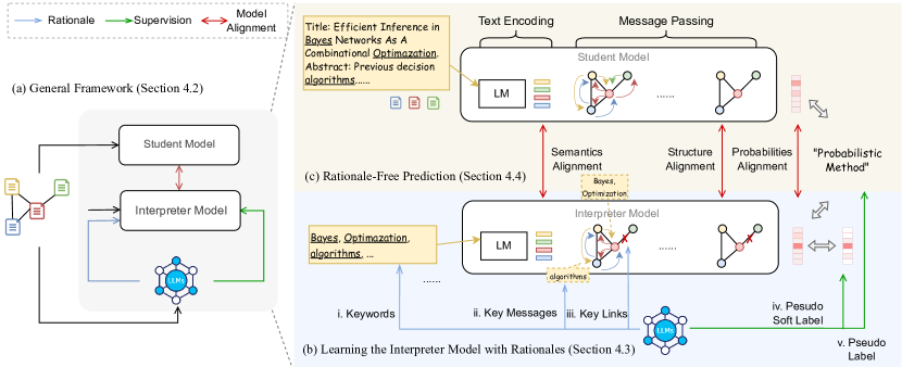
Figure 1: Illustration of our proposed LLM to graph model knowledge distillation framework. (a) The general distillation framework. (b) The training of the interpreter model with rationales and pseudo-supervision. (c) The proposed model alignment framework.

4.2 A General Framework for Distilling LLM to Graph Models

To tackle the difficulty in leveraging language models to teach graph models, we propose a framework that bridges the gap between these two types of models by enabling the student graph model to comprehend and apply the knowledge derived from LLMs.

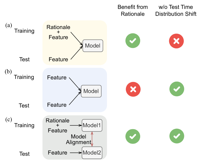
Figure 2: Different approaches to incorporate rationales to train graph models.

LLMs can provide rich knowledge on TAG learning, i.e., rationales. The rationales can be depicted as the important nodes, edges, and text features for each prediction. Graph models, which are discriminative models, can benefit from the rationales by taking them as input. Taking the rationales as input helps the model make predictions easier since the information in the rationale is exactly leading to the correct prediction. To make use of LLM’s knowledge, a naive idea is to use LLM-provided rich knowledge as additional features to train the graph model (Fig. 2 (a)). However, although the rationales can benefit the training process, using them as inputs to train the model leads to even worse test performance due to the distribution shift of features at the test time Wu et al. (2022). An alternative solution is to only leverage succinct knowledge (i.e. LLM’s predictions) as supervision to train the model so that the training and test features can be in the same distribution (Fig. 2 (b)). However, this method falls short of leveraging the full rationale power of LLMs, which encompasses rich information crucial for the student model’s understanding of the predictions.

To address this problem and ensure the model can be generalized to original features without rationales at test time, we propose a solution which is first to use LLMs’ rationale to train an intermediate model, then use the interpreter to train the student model with the same architecture but takes raw features without LLMs’ rationales as input (Fig. 2 (c)).

Leveraging this idea in knowledge distillation, we propose a novel framework for the LLM-to-graph model knowledge distillation problem, illustrated in Fig. 1 (a). Our proposed framework involves an intermediate Interpreter model, which bridges the LLM and the student model. Specifically, to extract the knowledge of LLMs on TAG learnings, we let LLMs provide rationales (the blue arrow) to enhance the features and provide supervision (the green arrow) to train the model. Since the interpreter model and the student model share a similar model structure, the student model can be aligned with the teacher model by aligning their latent embeddings (the red arrow).

Given this general framework, several specific questions arise that need to be addressed to enhance its practical application. These include: (1) how to incorporate LLM-generated textual rationales into the interpreter model, and (2) how to effectively align the student model with the interpreter model. The remainder of this paper addresses these questions, with the first question discussed in Section 4.3 and the second in Section 4.4.

4.3 Interpreter Model: Zero-Shot TAG Learning with Rationales

To tackle the difficulty in transferring text rationales to graph rationales, in this section we propose a new method to transfer TAG rationales into multiple-level enhanced features. The goal is to train the interpreter model, consisting of $LM^{\mathcal{T}}$ and $GNN^{\mathcal{T}}$.

The rationales behind a TAG model decision can be depicted as the prediction is primarily made based on which part(s) of text on which neighbor node(s). Since the graph models cannot directly take the textual rationales, to bridge the style of textual and graph rationales, we convert the textual rationale into three forms of feature enhancements that help with the prediction of the answer: i) keywords in texts, ii) key links around the central node, and iii) key semantic messages from the neighbors. To operationalize the training, we leverage LLMs to generate supervision to train the interpreter model, including iv) pseudo-soft labels and v) pseudo-labels. The training of the interpreter model with rationales is illustrated in Fig. 1 (b).

We prompt such prediction and reasoning in a three-step manner: 1) We input the text attributes of each node, along with those of its neighbors, into LLMs to generate pseudo-labels and pseudo-soft labels. 2) We then supply the node’s text and its pseudo-label to LLMs to identify critical keywords within the node’s attributes for the classification. 3) We feed the text of the node and its neighbors along with its pseudo-label into LLMs to identify essential links and messages for the classification. Each of these steps will be introduced in detail in the following. Examples of all prompts we used are given in Appendix C.

Pseudo-Label and Soft Label Creation. Since soft labels can have more information compared to hard categories in knowledge distillation Lopez-Paz et al. (2015), we first leverage the zero-shot abilities of LLMs to generate the pseudo-labels and pseudo-soft labels to assist in the training of the interpreter model. The generated labels are also used as the targeted answers for generating rationales. The process of label and soft-label creation can be written as

$$y_{n},l_{n}=LLM(x_{n},\{x_{i}\}_{\{i|v_{i}\in\mathcal{N}(v_{n})\}};prompt_{L})$$ (3)

where $y_{n}$ and $l_{n}$ are the LLM-predicted pseudo-label and soft label for node $v_{n}$, respectively. $LLM(x_{n},\{x_{i}\}_{\{i|v_{i}\in\mathcal{N}(v_{n})\}};prompt_{L})$ means calling LLM with the prompt $prompt_{L}$ and variables $x_{n}$ and $\{x_{i}\}_{\{i|v_{i}\in\mathcal{N}(v_{n})\}}$. The format conversion from textual outputs to numerical values is omitted in the mathematical expression.

Keyword Recognition. LLMs have been proven to have the capability to extract keywords in languages Hajialigol et al. (2023). In the interpreter model, we leverage the reasoning power of LLMs to extract the important keywords that are most helpful for the classification of the text, thus removing the words that can be noisy for classification. We then concatenate the keywords and feed them to the local $LM$ to extract text embeddings. Formally, assuming $prompt_{KW}$ is the prompt for keyword recognition, for a node $v_{n}$ with a text attribute $x_{n}$, we feed it to an LLM with $prompt_{KW}$ to obtain the recognized keywords. The enhanced text embedding can be obtained as

$$e_{n}^{\mathcal{T}}=LM^{\mathcal{T}}\left([LLM(x_{n},y_{n};prompt_{KW})]\right)$$ (4)

where $LLM(x_{n},y_{n};prompt_{KW})$ means utilizing LLMs to extract a list of important keywords of $x_{n}$ that helps to classify it to $y_{n}$ with the prompt $prompt_{KW}$. Here the output of the function $LLM$ with $prompt_{KW}$ is seen as the set of keywords. $[\cdot]$ denotes concatenating the keywords with spaces as the separator.

Key Links and Messages Recognition. For structural reasoning, we ask LLM to identify the key links around a specific central node by identifying a subset of neighbors (key links), and also the keywords in each of the neighbor nodes (key messages), that are important for the central node’s classification. The identified key links are used as edited local structures in message passing, and the key messages are used to replace the messages in the first graph convolutional layer. Formally, for a central node $v_{n}$, we provide $LLM$ with its text attribute $x_{n}$, its neighbors’ texts $\{x_{i}\}_{\{i|v_{i}\in\mathcal{N}(v_{n})\}}$, the pseudo-label $y_{n}$ and the prompt for this task $prompt_{KL}$, and extract the important neighbor set and keyword set from LLM’s response. For expression simplicity, we write them as the function $LLM$’s two outputs with $prompt_{KL}$. The key links and message recognition are written as

$$\mathcal{N}^{\prime}(v_{n}),\{{w}_{n,i}\}_{\{i|v_{i}\in\mathcal{N^{\prime}}(v_{n})\}}$$ (5)

$$=LLM\left(x_{n},\{x_{i}\}_{\{i|v_{i}\in\mathcal{N}(v_{n})\}},y_{n};prompt_{KL}\right)$$

where $\mathcal{N}^{\prime}(v_{n})$ is the key neighbor nodes and ${w}_{n,i}$ is the keywords in the message from node $v_{i}$ to the central node $v_{n}$. With the enhanced structural features, the message passing is done by

$$h_{n,k}^{\mathcal{T}} =\text{UPD}\big{(}h_{n,k-1}^{\mathcal{T}},$$ (6)

$$\text{AGG}(\{\text{MSG}(h_{n,k-1}^{\mathcal{T}},h_{m,k-1}^{\mathcal{T}})|v_{m}\in\mathcal{N}^{\prime}(v_{n})\})\big{)}$$

The messages in the first graph convolutional layer are replaced with

$$\text{MSG}(h_{n,k-1}^{\mathcal{T}},h_{i,k-1}^{\mathcal{T}})=LM^{\mathcal{T}}\left([w_{n,i}]\right)$$ (7)

where $[\cdot]$ denotes concatenating the words in the key message from $v_{i}$ to $v_{n}$.

Training Objective of the Interpreter Model. After obtaining the last layer’s node embedding $h_{n,l}^{\mathcal{T}}$, the prediction of the teacher model is made by $\hat{t}_{n}^{\mathcal{T}}=MLP^{\mathcal{T}}(h_{n,l}^{\mathcal{T}})$, where $\hat{t}_{n}^{\mathcal{T}}$ is the predicted soft label. The teacher model is trained to predict the label, and soft labels in a multi-task manner. The overall loss function to train the interpreter model is given by:

$$l^{\mathcal{T}}=\sum_{\{n\}_{v_{n}\in\mathcal{V}_{train}}}\bigg{(}l_{label}^{\mathcal{T}}(\hat{t}_{n}^{\mathcal{T}},y_{n})+\lambda_{1}l_{logits}^{\mathcal{T}}(\hat{t}_{n}^{\mathcal{T}},l_{n})\bigg{)}$$ (8)

where $l_{label}$ is implemented with the Cross-Entropy (CE) loss, $l_{logits}$ and $l_{msg}$ are implemented with the Mean Square Error (MSE) loss, and $\lambda_{1}$ is a hyper-parameter.

4.4 Semantics and Structure-Aware TAG Model Alignment

To achieve better LLM-free prediction at test time, we propose a new model alignment method for TAGs, as illustrated in Fig. 1 (c). The proposed method jointly considers the textual embeddings (LM-generated) and structural embeddings (GNN-generated) between the interpreter and student models, thus allowing the student model to give similar predictions to the interpreter model.

Semantics Alignment. For semantic representation, we extract text embeddings from the interpreter model and student model with weights considering their occurrence frequency in the graph structures. We also focus more on those nodes whose LLM-extracted keywords are more different from their raw text when aligning them. Formally, the semantic alignment loss can be written as:

$$l_{semantic}^{\mathcal{S}}=\sum_{\{n\}_{v_{n}\in\mathcal{V}_{train}}}\frac{\text{Deg}(v_{n})}{\text{sim}_{t}(x_{n},x^{\mathcal{T}}_{n})}\cdot d(h^{\mathcal{S}}_{n,0},h^{\mathcal{T}}_{n,0})$$ (9)

where $\text{Deg}(v_{n})$ is the degree of $v_{n}$, $\text{sim}_{t}(x_{n},x^{\mathcal{T}}_{n})$ is the semantic similarity between the raw text feature and the LLM-enhanced text feature of node $v_{n}$, which can be calculated with the cosine similarity of their embeddings extracted from a pre-trained language model like Bert. $d(h^{\mathcal{S}}_{n,0},h^{\mathcal{T}}_{n,0})$ is the discrepancy between their text embeddings that we aim to align.

Structure Alignment. In structural alignment, we also focus more on those nodes with more discrepancy between the original structure and the enhanced structure. Since in our proposed method, the structure enhancement is done by selecting important neighbors from all neighbors, the discrepancy can be calculated as the difference of neighbor node numbers. Formally, the structural alignment loss can be written as:

$$l_{structural}^{\mathcal{S}}=\sum_{\{n\}_{v_{n}\in\mathcal{V}_{train}}}\frac{\text{Deg}(v_{n})}{\text{sim}_{s}(\mathcal{N}(v_{n}),\mathcal{N}^{\prime}(v_{n}))}\cdot d(h^{\mathcal{S}}_{n,l},h^{\mathcal{T}}_{n,l})$$ (10)

where $\text{sim}_{s}(\mathcal{N}(v_{n}),\mathcal{N}^{\prime}(v_{n}))$ measures the similarity between $v_{n}$’s original neighbor structure and its enhanced neighbor structure, calculated by $\text{sim}_{s}(\mathcal{N}(v_{n}),\mathcal{N}^{\prime}(v_{n}))=\frac{1}{|\mathcal{N}_{k}(v_{n})|-|\mathcal{N}^{\prime}_{k}(v_{n})|}$, and $d(h^{\mathcal{S}}_{n,l},h^{\mathcal{T}}_{n,l})$ is a measure of the distance of node embeddings, which we aim to minimize.

Table 1: Main Results of Zero-Shot Test-Time LLM-Free Node Classification. The best performance on each dataset is bolded, and the second-best performance is underlined.

LLM’s Role	Type	Feature	Model	Cora	PubMed	ogbn-products	arxiv-2023
Annotator	LM	Text	Bert	0.7400±0.0175	0.9058±0.0046	0.7020±0.0033	0.6840±0.0122
			DistilBert	0.7355±0.0163	0.9028±0.0053	0.7080±0.0040	0.6821±0.0100
			Deberta	0.7385±0.0127	0.9020±0.0057	0.7074±0.0056	0.6789±0.0185
	GNN	Shallow	GCN	0.7126±0.0213	0.8322±0.0076	0.5593±0.0031	0.6355±0.0032
			GAT	0.7186±0.0346	0.8122±0.0282	0.5583±0.0010	0.6351±0.0060
			SAGE	0.7149±0.0223	0.8287±0.0107	0.5475±0.0023	0.6460±0.0006
		Text (PLM)	GCN	0.6720±0.0333	0.8136±0.0099	0.6944±0.0111	0.6647±0.0068
			GAT	0.6628±0.0434	0.7996±0.0229	0.7049±0.0043	0.6675±0.0059
			SAGE	0.6619±0.0191	0.7968±0.0118	0.6879±0.0067	0.6748±0.0067
		Text (FLM)	GCN	0.8090±0.0174	0.9043±0.0091	0.7300±0.0033	0.7655±0.0455
			GAT	0.8058±0.0320	0.8956±0.0099	0.7251±0.0013	0.7711±0.0479
			SAGE	0.8196±0.0294	0.9199±0.0105	0.7157±0.0047	0.7911±0.0521
Teacher (Proposed)	GNN	Text	GCN	0.8237±0.0187	0.9215±0.0096	0.7333±0.0025	0.7801±0.0424
			GAT	$\mathbf{0.8237}$±$\mathbf{0.0137}$	0.9189±0.0019	$\mathbf{0.7346}$±$\mathbf{0.0030}$	0.7838±0.0424
			SAGE	0.8210±0.0296	$\mathbf{0.9217}$±$\mathbf{0.0105}$	0.7283±0.0015	$\mathbf{0.7918}$±$\mathbf{0.0456}$

Overall Model Alignment Objective. In addition to the above two distillation loss functions, we also align the logits between the interpreter and the student model. The overall objective in model alignment can be written as:

$$l^{\mathcal{S}}=\underbrace{l_{label}^{\mathcal{S}}+\lambda_{2}l_{logits}^{\mathcal{S}}}_{\text{standard distillation}}+\underbrace{\lambda_{3}l_{semantic}^{\mathcal{S}}+\lambda_{4}l_{structural}^{\mathcal{S}}}_{\text{TAG model alignment}}$$ (11)

where $l_{label}^{\mathcal{S}}$ is the prediction loss of the student model, which is usually calculated with cross-entropy loss. $l_{logits}^{\mathcal{S}}$ is the logits alignment loss between the interpreter and student model, which is usually implemented with the mean square error (MSE) loss. $\lambda_{2},\lambda_{3},\lambda_{4}$ are the hyper-parameters.

5 Experiments

5.1 Experimental Setting

Datasets. We evaluate our proposed framework on four text-attributed graph datasets: Cora McCallum et al. (2000), Pubmed Sen et al. (2008), ogbn-products Hu et al. (2020) and arxiv-2023 He et al. (2023). We use the same subset of ogbn-products as in He et al. (2023). Specifically, we use the 2023 version Arxiv He et al. (2023) which is a dataset comprising papers published in 2023 or later, beyond the knowledge cutoff for GPT-3.5, to address the concern of potential label leakage. The detailed information of each dataset is given in Appendix A.

Baseline Methods. We compare our proposed method with only distilling the prediction without rationales (LLMs as Annotators) on LMs and GNNs. For LMs, we use Bert Devlin et al. (2018), DistilBert Sanh et al. (2019) and DeBERTa He et al. (2020) as backbones; for GNNs, we tested GCN Kipf and Welling (2016), GAT Veličković et al. (2017) and GraphSAGE Hamilton et al. (2017) as backbones, and tested shallow embeddings in the PyG library Fey and Lenssen (2019) (denoted as Shallow), pre-trained language models’ provided text embeddings (denoted as PLM) and fine-tuned LMs’ text embeddings (denoted as FLM) as initial node features. We use GPT-3.5 Turbo in all LLM-related scenarios.

Training and Implementation Details. We follow the standard inductive learning setting Zhang et al. (2021), all links between the training nodes and test nodes in the graphs are removed in the training stage to ensure all test nodes are unseen during training. More implementation details are given in Appendix B.

5.2 Main Results of Zero-Shot Test Time LLM-Free Node Classification

We first compare our proposed method with other test-time LLM-free TAG learning methods. The main results are shown in Table 1. Generally, our proposed framework achieves the best performance on all datasets, and our proposed method can give an increased performance for all GNN backbones.

Best performance on all datasets. Our proposed method achieves the best scores on all datasets, demonstrating its general efficacy. Moreover, for each GNN backbone, our proposed method yields a $1.3\%$ performance improvement on Cora, $1.4\%$ improvement on PubMed, $0.87\%$ improvement on ogbn-products and $0.93\%$ improvement on arxiv-2023, showing our proposed method can consistently beat the all the baseline methods with significant improvements.

Consistent improvements over all GNN backbones. Among all baseline methods, using fine-tuned language models to extract initial node features and then apply GNNs for classification (denoted by Text (FLM) in Table 1) gives the best performance. Compared with this method, our proposed method can achieve improvements on all datasets and all GNN backbones. For example, although the second-best performance is achieved by the baseline SAGE backbone with Text (FLM) as node features, our method still achieves improvements on all GNN backbones under a pair-wise comparison of each GNN backbone.

Potential as pre-training in standard supervised learning. We also demonstrate that our proposed framework can be used as an effective model pre-training method when the downstream task is a standard supervised learning setting on the same data. We conducted experiments on Cora dataset to validate the performance increase. The results are shown in Table. 2. Results reveal that the proposed distillation can serve as an effective model pre-training in the supervised learning setting. It is worth noting that this pre-training uses the same set of TAG data as the supervised learning setting.

Table 2: Performance comparison between standard supervised learning and using proposed method as model pre-training on Cora dataset

Method	GCN	GAT	SAGE
w/o Pre-training	0.8778±0.0084	0.8750±0.0137	0.8815±0.0093
w/ Pre-training	0.8882±0.0020	0.8813±0.0015	0.8910±0.0028

5.3 Ablation Study of Interpreter Model’s Feature Enhancements

We conduct an ablation study of each enhanced feature on Cora dataset. The results are shown in Table 3. To construct ablated versions, we remove the LLM-generated soft labels as supervision (w/o soft labels), keywords recognition (w/o keywords), key edges recognition (w/o key edges), and key messages (w/o messages), correspondingly. The results validate the effectiveness of each feature enhancement for the interpreter model. Specifically, the results show that the proposed method with all components achieves the best average performance (ranked first). This reveals using full components can lead to a more reliable performance. The results also reveal that key edges and LLM-generated messages play a relatively larger role in the interpreter model’s performance improvement, which is aligned with the nature of TAGs that structure-related information plays a more important role than pure text information.

Table 3: Ablation study on feature enhancements, showing interpreter model accuracy. Performances are distinguished: best, second, and third. Includes a Rank column for average accuracy ranking across three GNN backbones.

Method	GCN	GAT	SAGE	Rank
Baseline	0.8090±0.0174	0.8058±0.0320	0.8196±0.0294	6
w/o soft labels	0.8310±0.0376	0.8292±0.0451	$\mathbf{0.8369}$±$\mathbf{0.0527}$	3
w/o keywords	0.8363±0.0291	0.8344±0.0288	0.8322±0.0312	2
w/o key edges	0.8247±0.0271	0.8215±0.0302	0.8353±0.0494	5
w/o messages	$\mathbf{0.8379}$±$\mathbf{0.0388}$	0.8233±0.0410	0.8296±0.0538	4
Proposed	0.8336±0.0288	$\mathbf{0.8376}$±$\mathbf{0.0209}$	0.8326±0.0210	1

Table 4: Ablation study of proposed feature discrepancy feature alignment. The method Interpreter denotes the performance of the interpreter model, which is the target for the student model to emulate through alignment.

Method	GCN	GAT	SAGE
Interpreter	0.8336±0.0288	0.8376±0.0209	0.8326±0.0210
Baseline	0.8090±0.0174	0.8058±0.0320	0.8196±0.0294
Proposed-T	0.8127±0.0235	0.8104±0.0157	0.8187±0.0307
Proposed-N	0.8146±0.0196	0.8081±0.0116	0.8204±0.0304
Proposed	$\mathbf{0.8237}$±$\mathbf{0.0187}$	$\mathbf{0.8237}$±$\mathbf{0.0137}$	$\mathbf{0.8210}$±$\mathbf{0.0296}$

5.4 Ablation Study of Discrepancy-Aware Model Alignment

We further study the effectiveness of two proposed model alignment terms on the Cora dataset. The results are shown in Table 4. In this experiment, the baseline method (denoted by "Baseline") is vanilla model alignment by minimizing the soft predictions, "Proposed-T" and "Proposed-N" means removing the term of semantics and structure alignment, correspondingly. Results show that the proposed method consistently beat all the ablation versions, thus validating the effectiveness of the two proposed alignment terms. Also, the narrower performance gap between the student model and the teacher model shows our proposed framework can well infer unseen data with a consistent performance compared to when LLMs are available.

5.5 Parameter Sensitivity Analysis

We explore the sensitivity of the hyper-parameters in our framework, namely $\lambda_{1}$, $\lambda_{2}$, $\lambda_{3}$, $\lambda_{4}$. For each hyper-parameter, we train the model on seven values ranging from 0.001 to 10, and test the performance of node classification accuracy. Experiments are done on Cora dataset with GCN as the model backbone. The results are shown in Fig. 3. Generally, the results demonstrated the robustness of the proposed framework against the varying of its hyper-parameters. To be more specific, the two parameters corresponding to our proposed alignment terms, $\lambda_{2}$ and $\lambda_{3}$, show a higher stability of the model performance against the change of their values. That shows the stableness of our proposed discrepancy-aware alignment. The parameter $\lambda_{1}$, which corresponds to the loss calculated between the teacher model predicted soft labels and LLM-generated soft labels shows a large performance drop when its value reaches 10. This can be explained as the LLM-generated soft labels are not always reliable.

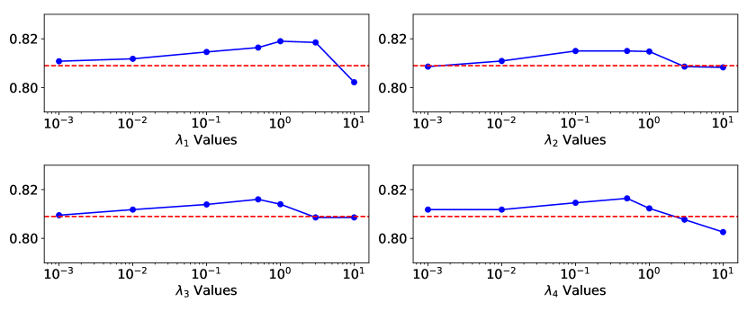
Figure 3: Sensitivity analysis of parameters $\lambda_{1}$, $\lambda_{2}$, $\lambda_{3}$ and $\lambda_{4}$. The red line denotes the baseline performance.

6 Conclusion

In this paper, we propose a framework to distill LLMs to graph models on TAG learning which allows training with both predictions and rationales. We train an interpreter model to bridge LLM’s rationale to the graph model and align the interpreter model based on the nature of TAG data. On four datasets, our proposed distillation method overperforms the baseline by an average of 1.25%.

Limitations

Our method, which aims to distill LLMs for TAG learning, is influenced by the design of prompts for the LLM, potentially affecting the quality of generated rationales. The capabilities of LLMs also influence the correctness of the prediction and rationales. High-capability LLMs, such as GPT-3.5 and GPT-4, are required for our distillation framework to generate reasonable rationales.

Ethical Statements

The datasets and model we used are all open-source and all the references that draw on the work of others are marked with citations. In the process of constructing the rationales and pseudo-supervision, we ensure that all the triples come from GPT-3.5 Turbo, a publicly available LLM. There are no ethical issues in this work. ChatGPT is partially used for coding and checking the grammar in this paper.

Appendix A Dataset Details

Table 5: Statistics of the TAG datasets

Dataset	#Nodes	#Edges	#Classes
Cora	2,708	5,429	7
Pubmed	19,717	44,338	3
ogbn-products	54,025	74,420	47
arxiv-2023	46,198	78,548	40

The details of each dataset in shown in Table 5. Following previous work He et al. (2023), for all datasets, we randomly split the training/validation/test set with the ratio of 60/20/20.

Appendix B Implementation Details

The implementation of the proposed method utilized the PyG and Huggingface libraries, which are licensed under the MIT License. All experiments were conducted on a single NVIDIA RTX 3090 GPU with 24GB VRAM. For pre-training language models, we use a max token number of 512 for full-text features and 48 for keyword features for all three pre-trained language models including bert-base-uncased, distilbert-base-uncased, and microsoft/deberta-base. For the GNN models including GCN, GAT and SAGE, we test on 2-layer models with a hidden dimension of 256. In the training process, we first train the interpreter model alone until convergence, then fix the interpreter model to train the student model. The interpreter model is trained first, then we freeze it and train the student model. We adopt a learning rate of 1e-5 to fine-tune all the pre-trained language models and train for 10 epochs. We train all GNN models for 200 epochs with a learning rate of 0.01.

Appendix C Prompt Details

OpenAI’s GPT-3.5 Turbo 1103 version is utilized in all experiments. Especially, for the ogbn-products and arxiv-2023 datasets, since the total number of categories is large, we adjust the prompt for generating pseudo-soft labels to only generate for the top-5 probable classes, instead of all classes. The complete prompt examples for each dataset and example replies can be found in the following. $prompt_{L}$ has two versions, one for Cora and Pubmed, the other for Arxiv and Products datasets. The two other prompts are the same across all datasets, only different in the options of categories of each dataset. All the prompt examples are shown in Table 6.

Table 6: Prompt Details

Prompt	Content
$prompt_{KL}$	We are exploring a citation network. Each node is associated with a paper’s title and abstract. Each node belongs to one of the classes of [….] Now I want to do the classification of a node. I will give you the class and text of central node and its neighbor nodes. Please identify a subset of the neighbor nodes that the link between central node and them may help a correct classification of the central node, and a set of at most five important single keywords in each important neighbor node that are important to classify the central node’s category. The key words should also be common and general across all potential text from this class. For example: Information I give you: Central Node, Class: Neural_Networks, Text: Title: Graph Neural Networks for molecule design. Abstract: This paper presents a novel Graph Neural Network model for molecule generation. Neighbors: Node 2: Title: Machine Learning For Health: A Review. Abstract: This paper presents a systematic survey of using Deep Learning models for Health prediction. In this example, your reply should be a json like: {’Node 2’: [’Machine’, ’bayesian’, ’prediction’]}. You should only give the keywords for the Neighbors which you think are important to classify the central node. Do not reply anything else except this json. Now, the case you should study is:
$prompt_{KW}$	We are exploring a citation network. Each node is associated with a paper’s title and abstract. Each node belongs to one of the classes of [….] Now I want to do the classification of a node. I will give you the class and text of central node. Please identify up to 5 keywords in the text that may help a correct classification of the central node. The key words should also be common and general across all potential text from this class. For example: Information I give you: Central Node, Class: Neural_Networks, Text: Title: Graph Neural Networks for molecule design. Abstract: This paper presents a novel Graph Neural Network model for molecule generation. In this example, your reply should be a json like: {’Important Keywords’: [’Neural’, ’Network’]}. Do not reply anything else except this json. Now, the case you should study is:
$prompt_{L}$ - ogbn-products and arxiv-2023	We are exploring a product. Each node is assiciated with a product’s description Each node belongs to one of the classes of [….]. Now I want to do classification of a node. Give a logits-like probabilities of how likely it will be in each of your provided top-five probable classes (sum to be 1). Finally your predicted class. Your identified highest probability class must be consistent with the highest probability in your provided logits. For example, your reply format should be like: { "Likely Classes": ["Digital Music", "Office Products", …], "Logits": [0, 0, 0.7, 0.2, 0.1], "Predicted Class": "Digital Music"}. In your likely classes, please strictly follow the format I gave you for each class name. Do not reply anything else except strictly follow this json format. Makesure all the classes are in the classed I gave you. You can reply less than 5 classes. Now the text you should deal with is:
$prompt_{L}$ - Cora and Pubmed	We are exploring a citation network. Each node is assiciated with a paper’s title and abtract. Each node belongs to one of the classes of [….]. Now I want to do classification of a node. Give a logits-like probabilities of how likely it will be in each of these classes [….] (sum to be 1). Finally your predicted class. For example: Text: Deep neural networks methods for biological discovery. Your reply: "{"Logits": [0, 0, 0.7, 0.2, 0.1, 0, 0], "Predicted Class": "Neural_Networks"}". Now the text you should deal with is:

References

- Chen et al. (2023a) Zhikai Chen, Haitao Mao, Hang Li, Wei Jin, Hongzhi Wen, Xiaochi Wei, Shuaiqiang Wang, Dawei Yin, Wenqi Fan, Hui Liu, et al. 2023a. Exploring the potential of large language models (llms) in learning on graphs. arXiv preprint arXiv:2307.03393.
- Chen et al. (2023b) Zhikai Chen, Haitao Mao, Hongzhi Wen, Haoyu Han, Wei Jin, Haiyang Zhang, Hui Liu, and Jiliang Tang. 2023b. Label-free node classification on graphs with large language models (llms). arXiv preprint arXiv:2310.04668.
- Chien et al. (2021) Eli Chien, Wei-Cheng Chang, Cho-Jui Hsieh, Hsiang-Fu Yu, Jiong Zhang, Olgica Milenkovic, and Inderjit S Dhillon. 2021. Node feature extraction by self-supervised multi-scale neighborhood prediction. arXiv preprint arXiv:2111.00064.
- Dasgupta et al. (2023) Sayantan Dasgupta, Trevor Cohn, and Timothy Baldwin. 2023. Cost-effective distillation of large language models. In Findings of the Association for Computational Linguistics: ACL 2023, pages 7346–7354.
- Devlin et al. (2018) Jacob Devlin, Ming-Wei Chang, Kenton Lee, and Kristina Toutanova. 2018. Bert: Pre-training of deep bidirectional transformers for language understanding. arXiv preprint arXiv:1810.04805.
- Duan et al. (2023) Keyu Duan, Qian Liu, Tat-Seng Chua, Shuicheng Yan, Wei Tsang Ooi, Qizhe Xie, and Junxian He. 2023. Simteg: A frustratingly simple approach improves textual graph learning. arXiv preprint arXiv:2308.02565.
- Fey and Lenssen (2019) Matthias Fey and Jan E. Lenssen. 2019. Fast graph representation learning with PyTorch Geometric. In ICLR Workshop on Representation Learning on Graphs and Manifolds.
- Hajialigol et al. (2023) Daniel Hajialigol, Hanwen Liu, and Xuan Wang. 2023. Xai-class: Explanation-enhanced text classification with extremely weak supervision. arXiv preprint arXiv:2311.00189.
- Hamilton et al. (2017) Will Hamilton, Zhitao Ying, and Jure Leskovec. 2017. Inductive representation learning on large graphs. Advances in neural information processing systems, 30.
- He et al. (2020) Pengcheng He, Xiaodong Liu, Jianfeng Gao, and Weizhu Chen. 2020. Deberta: Decoding-enhanced bert with disentangled attention. arXiv preprint arXiv:2006.03654.
- He et al. (2023) Xiaoxin He, Xavier Bresson, Thomas Laurent, and Bryan Hooi. 2023. Explanations as features: Llm-based features for text-attributed graphs. arXiv preprint arXiv:2305.19523.
- Hinton et al. (2015) Geoffrey Hinton, Oriol Vinyals, and Jeff Dean. 2015. Distilling the knowledge in a neural network. arXiv preprint arXiv:1503.02531.
- Ho et al. (2022) Namgyu Ho, Laura Schmid, and Se-Young Yun. 2022. Large language models are reasoning teachers. arXiv preprint arXiv:2212.10071.
- Hsieh et al. (2023) Cheng-Yu Hsieh, Chun-Liang Li, Chih-Kuan Yeh, Hootan Nakhost, Yasuhisa Fujii, Alexander Ratner, Ranjay Krishna, Chen-Yu Lee, and Tomas Pfister. 2023. Distilling step-by-step! outperforming larger language models with less training data and smaller model sizes. arXiv preprint arXiv:2305.02301.
- Hu et al. (2020) Weihua Hu, Matthias Fey, Marinka Zitnik, Yuxiao Dong, Hongyu Ren, Bowen Liu, Michele Catasta, and Jure Leskovec. 2020. Open graph benchmark: Datasets for machine learning on graphs. Advances in neural information processing systems, 33:22118–22133.
- Huang et al. (2023) Jin Huang, Xingjian Zhang, Qiaozhu Mei, and Jiaqi Ma. 2023. Can llms effectively leverage graph structural information: when and why. arXiv preprint arXiv:2309.16595.
- Jiao et al. (2019) Xiaoqi Jiao, Yichun Yin, Lifeng Shang, Xin Jiang, Xiao Chen, Linlin Li, Fang Wang, and Qun Liu. 2019. Tinybert: Distilling bert for natural language understanding. arXiv preprint arXiv:1909.10351.
- Kipf and Welling (2016) Thomas N Kipf and Max Welling. 2016. Semi-supervised classification with graph convolutional networks. arXiv preprint arXiv:1609.02907.
- Li et al. (2023) Liunian Harold Li, Jack Hessel, Youngjae Yu, Xiang Ren, Kai-Wei Chang, and Yejin Choi. 2023. Symbolic chain-of-thought distillation: Small models can also" think" step-by-step. arXiv preprint arXiv:2306.14050.
- Li et al. (2022) Shiyang Li, Jianshu Chen, Yelong Shen, Zhiyu Chen, Xinlu Zhang, Zekun Li, Hong Wang, Jing Qian, Baolin Peng, Yi Mao, et al. 2022. Explanations from large language models make small reasoners better. arXiv preprint arXiv:2210.06726.
- Lopez-Paz et al. (2015) David Lopez-Paz, Léon Bottou, Bernhard Schölkopf, and Vladimir Vapnik. 2015. Unifying distillation and privileged information. arXiv preprint arXiv:1511.03643.
- Magister et al. (2022) Lucie Charlotte Magister, Jonathan Mallinson, Jakub Adamek, Eric Malmi, and Aliaksei Severyn. 2022. Teaching small language models to reason. arXiv preprint arXiv:2212.08410.
- McCallum et al. (2000) Andrew Kachites McCallum, Kamal Nigam, Jason Rennie, and Kristie Seymore. 2000. Automating the construction of internet portals with machine learning. Information Retrieval, 3:127–163.
- Sanh et al. (2019) Victor Sanh, Lysandre Debut, Julien Chaumond, and Thomas Wolf. 2019. Distilbert, a distilled version of bert: smaller, faster, cheaper and lighter. arXiv preprint arXiv:1910.01108.
- Sen et al. (2008) Prithviraj Sen, Galileo Namata, Mustafa Bilgic, Lise Getoor, Brian Galligher, and Tina Eliassi-Rad. 2008. Collective classification in network data. AI magazine, 29(3):93–93.
- Shridhar et al. (2023) Kumar Shridhar, Alessandro Stolfo, and Mrinmaya Sachan. 2023. Distilling reasoning capabilities into smaller language models. In Findings of the Association for Computational Linguistics: ACL 2023, pages 7059–7073.
- Sun et al. (2023) Shengyin Sun, Yuxiang Ren, Chen Ma, and Xuecang Zhang. 2023. Large language models as topological structure enhancers for text-attributed graphs. arXiv preprint arXiv:2311.14324.
- Vapnik et al. (2015) Vladimir Vapnik, Rauf Izmailov, et al. 2015. Learning using privileged information: similarity control and knowledge transfer. J. Mach. Learn. Res., 16(1):2023–2049.
- Veličković et al. (2017) Petar Veličković, Guillem Cucurull, Arantxa Casanova, Adriana Romero, Pietro Lio, and Yoshua Bengio. 2017. Graph attention networks. arXiv preprint arXiv:1710.10903.
- Wan et al. (2023) Zhongwei Wan, Xin Wang, Che Liu, Samiul Alam, Yu Zheng, Zhongnan Qu, Shen Yan, Yi Zhu, Quanlu Zhang, Mosharaf Chowdhury, et al. 2023. Efficient large language models: A survey. arXiv preprint arXiv:2312.03863, 1.
- Wang et al. (2021) Zheng Wang, Jialong Wang, Yuchen Guo, and Zhiguo Gong. 2021. Zero-shot node classification with decomposed graph prototype network. In Proceedings of the 27th ACM SIGKDD Conference on Knowledge Discovery & Data Mining, pages 1769–1779.
- Wu et al. (2022) Lirong Wu, Haitao Lin, Yufei Huang, and Stan Z Li. 2022. Knowledge distillation improves graph structure augmentation for graph neural networks. Advances in Neural Information Processing Systems, 35:11815–11827.
- Yao et al. (2023) Yifan Yao, Jinhao Duan, Kaidi Xu, Yuanfang Cai, Eric Sun, and Yue Zhang. 2023. A survey on large language model (llm) security and privacy: The good, the bad, and the ugly. arXiv preprint arXiv:2312.02003.
- Yue et al. (2022) Qin Yue, Jiye Liang, Junbiao Cui, and Liang Bai. 2022. Dual bidirectional graph convolutional networks for zero-shot node classification. In Proceedings of the 28th ACM SIGKDD Conference on Knowledge Discovery and Data Mining, pages 2408–2417.
- Zhang et al. (2021) Shichang Zhang, Yozen Liu, Yizhou Sun, and Neil Shah. 2021. Graph-less neural networks: Teaching old mlps new tricks via distillation. arXiv preprint arXiv:2110.08727.
- Zhao et al. (2022) Jianan Zhao, Meng Qu, Chaozhuo Li, Hao Yan, Qian Liu, Rui Li, Xing Xie, and Jian Tang. 2022. Learning on large-scale text-attributed graphs via variational inference. arXiv preprint arXiv:2210.14709.
- Zhu et al. (2021) Jason Zhu, Yanling Cui, Yuming Liu, Hao Sun, Xue Li, Markus Pelger, Tianqi Yang, Liangjie Zhang, Ruofei Zhang, and Huasha Zhao. 2021. Textgnn: Improving text encoder via graph neural network in sponsored search. In Proceedings of the Web Conference 2021, pages 2848–2857.