Direct Consistency Optimization for
Compositional Text-to-Image Personalization

Abstract

Text-to-image (T2I) diffusion models, when fine-tuned on a few personal images, are able to generate visuals with a high degree of consistency. However, they still lack in synthesizing images of different scenarios or styles that are possible in the original pretrained models. To address this, we propose to fine-tune the T2I model by maximizing consistency to reference images, while penalizing the deviation from the pretrained model. We devise a novel training objective for T2I diffusion models that minimally fine-tunes the pretrained model to achieve consistency. Our method, dubbed Direct Consistency Optimization, is as simple as regular diffusion loss, while significantly enhancing the compositionality of personalized T2I models. Also, our approach induces a new sampling method that controls the tradeoff between image fidelity and prompt fidelity. Lastly, we emphasize the necessity of using a comprehensive caption for reference images to further enhance the image-text alignment. We show the efficacy of the proposed method on the T2I personalization for subject, style, or both. In particular, our method results in a superior Pareto frontier to the baselines. See our project page for more examples and codes.

1 Introduction

Text-to-image (T2I) is a model for image generation guided by the natural language prompt and has seen rapid progress in recent years (Ramesh et al., 2021; Saharia et al., 2022; Ramesh et al., 2022; Rombach et al., 2022; Yu et al., 2022; Podell et al., 2023; Chang et al., 2023; Betker et al., 2023). The compositional nature of the natural language has enabled the creation of novel images, which composes multiple subjects with varying attributes at different backgrounds or styles. However, the ambiguity of natural language in describing the visual world makes it difficult to create an image of a specific subject, style, interaction, or background.

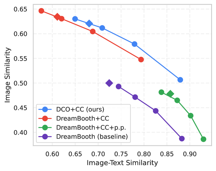
Figure 1: Pareto curve between subject fidelity (image similarity) and compositionality (image-text similarity) on subject personalization task of T2I diffusion models. Scores of each point on the curve are measured with different values of reward guidance sampling ($\bullet$), in addition to a classifier-free guidance sampling ($\blackdiamond$). Top-right corner is preferred. Our method, Direct Consistency Optimization (DCO), with the Comprehensive Caption (CC), pushes the frontier to the upper-right over DreamBooth (Ruiz et al., 2023a), with CC (DreamBooth+CC), and with prior preservation loss (DreamBooth+CC+p.p.). Appendix B for full comparison.

To overcome the lack of accuracy in natural language, there has been an emerging interest in teaching the pretrained T2I models new concepts, such as subject (Gal et al., 2022; Ruiz et al., 2023a), style (Sohn et al., 2023), interaction (Huang et al., 2023), or background (Tang et al., 2023), whose precise visual description is given by a small set of reference images. As proposed in DreamBooth (DB) (Ruiz et al., 2023a), the fundamental idea is to fine-tune the pretrained T2I model on a few images describing a new concept. The adoption of LoRA (Hu et al., 2021) or adapter fine-tuning (Houlsby et al., 2019) to T2I models has made the process more accessible, fast and economical (Ryu, 2023; Sohn et al., 2023). Once fine-tuned, the model can generate images by composing a new concept (e.g., my subject) and the knowledge of the pretrained model (e.g., background, style). While these methods have shown great success, they still suffer from reduced textual alignment and compositional generation capability (Arar et al., 2024), which is particularly problematic when the number of reference images is few. As in Fig. 1, though the subject consistency to reference images, measured by the image similarity, is improved with DreamBooth (${\color[rgb]{0.40234375,0.2265625,0.71875}\blackdiamond}\,0.500$ vs. $0.308$), this comes at a cost of vastly reduced image-text similarity over the pretrained T2I model (${\color[rgb]{0.40234375,0.2265625,0.71875}\blackdiamond}\,0.724$ vs. $0.895$). Ideally, we should aim for high image-text and image similarities after fine-tuning (e.g., top-right corner).

We hypothesize that the limitation comes from the knowledge forgetting (e.g., fails to compose my subject in a known style) and concept collapse (e.g., background concept gets subsumed into my subject) that happened during the course of low-shot fine-tuning. In this work, we aim to develop a method that mitigates such forgetting behavior for low-shot fine-tuning of T2I diffusion models. To this end, we propose Direct Consistency Optimization (DCO), where we fine-tune diffusion models by casting it as a constrained policy optimization problem (Peters et al., 2010; Wu et al., 2019), that promotes text-to-image model to learn the minimal information without losing the composition ability of the pretrained model. Moreover, as DCO encourages each fine-tuned model to be consistent with the pretrained model, two independently fine-tuned models on separate concepts can be easily merged for a multi-concept personalized image generation. We also present a guidance method that balances subject consistency and textual alignment, which allows users to control their preferences. Last but not least, we emphasize the importance of comprehensive and visually grounded captions for low-shot fine-tuning as a way of preventing model shift and concept collapse.

We conduct an extensive empirical study on the personalization of T2I diffusion models. We show that the proposed method improves upon strong baselines including DreamBooth (Ruiz et al., 2023a) and its combination with Textual Inversion (Gal et al., 2022) in the compositional generation of a custom subject with the known style of the pretrained model. Moreover, our approach is applied to the style customization (Sohn et al., 2023) and the composition of independently fine-tuned subject and style T2I models to create an image of my subject in my style (Sohn et al., 2023) without an additional optimization as in (Shah et al., 2023).

2 Related Work

We briefly review the literatures on personalized T2I synthesis and fine-tuning of T2I diffusion models with rewards. A more comprehensive review of relevant work is in Sec. C.

Personalized T2I synthesis.  Several works have shown the promise of personalized T2I synthesis from a few images (Gal et al., 2022; Ruiz et al., 2023a; Han et al., 2023; Kumari et al., 2023; Sohn et al., 2023). To improve efficiency, parameter efficient fine-tuning (PEFT) methods such as soft prompt tuning (Gal et al., 2022; Wei et al., 2023; Gal et al., 2023; Voynov et al., 2023; Tewel et al., 2023), LoRA (Hu et al., 2021; Ruiz et al., 2023b) and adapter tuning (Houlsby et al., 2019; Sohn et al., 2023), have been proposed. To preserve the prior knowledge, Ruiz et al. (2023a) proposed prior preservation loss, which additionally fine-tunes on a class-specific prior dataset synthesized from pretrained T2I model. We present a different approach to preserve prior knowledge by regularizing the model with pretrained model without using any prior dataset.

Fine-tuning T2I diffusion models with rewards.  A line of works has studied fine-tuning T2I diffusion models using reward models such as human preferences (Lee et al., 2023; Kirstain et al., 2023; Xu et al., 2023) or aesthetic scores (Schuhmann & Beaumont, 2022). Those methods use auxiliary reward models to update diffusion models by weighting with rewards (Lee et al., 2023), use reinforcement learning algorithms (Fan et al., 2023; Black et al., 2023), or differentiate through the reward models (Dong et al., 2023; Clark et al., 2023; Prabhudesai et al., 2023). On the other hand, Wallace et al. (2023) have adapted direct preference optimizaton (Rafailov et al., 2023) to fine-tune T2I models with paired preference dataset which do not require explicit reward models. To our knowledge, we are the first to study consistency as a reward function for T2I personalization, or low-shot fine-tuning of T2I diffusion models.

3 Preliminaries

T2I diffusion models. Let $q(\mathbf{x})$ be the data distribution and $p_{\theta}(\mathbf{x})$ be a generative model parameterized by $\theta$ that approximates $q$. The denoising diffusion model (Ho et al., 2020) gradually adds the Gaussian noise to a sample $\mathbf{x_{0}}\sim q(\mathbf{x})$, forming a sequence of latent variables that leads to a joint distribution $q(\mathbf{x}_{0:T})=q(\mathbf{x}_{0},\dots,\mathbf{x}_{T})=q(\mathbf{x}_{0})\Pi_{t=1}^{T}q(\mathbf{x}_{t}|\mathbf{x}_{t-1})$. More formally, the marginal distribution $q_{t}(\mathbf{x}_{t})$ at timestep $t\in[0,T]$ is given by $\mathbf{x}_{t}=\alpha_{t}\mathbf{x}_{t-1}+\sigma_{t}\boldsymbol{\varepsilon},$ where $\boldsymbol{\varepsilon}\sim\mathcal{N}(\boldsymbol{0},\mathbf{I})$, and $\alpha_{t},\sigma_{t}>0$ are noise-scheduling functions. For $\sigma_{T}\gg\sigma_{0}$, $\mathbf{x}_{T}$ is indistinguishable from pure Gaussian noise. Then the diffusion model samples a random noise $\mathbf{x}_{T}\sim\mathcal{N}(\boldsymbol{0},\sigma_{T}^{2}\mathbf{I})$, and sequentially denoise it for recovering $\mathbf{x}_{t}$, so that the recovered one for $\mathbf{x}_{0}$ matches the original data distribution $q(\mathbf{x}_{0})$. In theory, the generative sampling process is governed by solving SDE (Song et al., 2020b; Ho et al., 2020) or probability flow ODE (Song et al., 2020a; Karras et al., 2022), using the score function of marginal data distribution $\nabla\log q_{t}(\mathbf{x}_{t})$. The training objective of the diffusion model is characterized as minimizing the upper bound of KL divergence $D_{\textrm{KL}}\big{(}q(\mathbf{x}_{0})\,\|\,p_{\theta}(\mathbf{x}_{0})\big{)}$, given as

$$D_{\textrm{KL}}\big{(}q(\mathbf{x}_{0})\,\|\,p_{\theta}(\mathbf{x}_{0})\big{)}\leq D_{\textrm{KL}}\big{(}q(\mathbf{x}_{0:T})\,\|\,p_{\theta}(\mathbf{x}_{0:T})\big{)}\text{,}$$ (1)

which is equivalent to the weighted denoising score matching (DSM) objective (Hyvärinen & Dayan, 2005) that approximates the score function $\nabla\log q_{t}(\mathbf{x}_{t})$ of marginal distribution at each timestep $t$ (Kingma & Gao, 2023).

T2I diffusion models (Nichol et al., 2021; Saharia et al., 2022; Rombach et al., 2022) are diffusion models of an image conditioned on text, which is often processed into embeddings using the pretrained text encoders, such as T5 (Raffel et al., 2020) or CLIP (Radford et al., 2021). Given a dataset $(\mathbf{x},\mathbf{c})\sim\mathcal{D}$ of paired image $\mathbf{x}$ and text prompt $\mathbf{c}$, T2I diffusion models are often parametrized through a noise-prediction model $\boldsymbol{\varepsilon}_{\theta}(\mathbf{x}_{t};\mathbf{c},t)$ that estimates the scaled score function $-\sigma_{t}\nabla_{\mathbf{x}_{t}}\log q_{t}(\mathbf{x}_{t}|\mathbf{c})$. The corresponding noise-prediction loss (Ho et al., 2020; Rombach et al., 2022) is equivalent to the DSM objective, which is given as follows:

$$\mathcal{L}_{\textrm{DM}}(\theta;\mathcal{D})=\mathbb{E}_{(\mathbf{x},\mathbf{c})\sim\mathcal{D},\boldsymbol{\varepsilon},t}\big{[}\omega(t)\|\boldsymbol{\varepsilon}_{\theta}(\mathbf{x}_{t};\mathbf{c},t)-\boldsymbol{\varepsilon}\|_{2}^{2}\big{]}\text{,}$$ (2)

where $\mathbf{x}_{t}=\alpha_{t}\mathbf{x}_{t-1}+\sigma_{t}\boldsymbol{\varepsilon}$ for $\boldsymbol{\varepsilon}\sim\mathcal{N}(\boldsymbol{0},\mathbf{I})$, $t\sim\mathcal{U}(0,T)$, and $\omega(t)$ is a weighting function at each timestep $t$. To obtain effective text conditioning, T2I models are trained with classifier-free guidance (CFG) (Ho & Salimans, 2022), which jointly learns unconditional and conditional models, and interpolates them during inference. The predicted noise interpolated by CFG scale $\omega\geq 1$ is given as:

$$\hat{\boldsymbol{\varepsilon}}_{\theta}(\mathbf{x}_{t};\mathbf{c},t)=\omega\,(\boldsymbol{\varepsilon}_{\theta}(\mathbf{x}_{t};\mathbf{c},t)-\boldsymbol{\varepsilon}_{\theta}(\mathbf{x}_{t};t))+\boldsymbol{\varepsilon}_{\theta}(\mathbf{x}_{t};t)\text{,}$$ (3)

where $\boldsymbol{\varepsilon}_{\theta}(\mathbf{x}_{t};t)$ denotes the noise with null text embeddings. Note that one can use negative prompts instead of null prompt for additional control (Liu et al., 2022).

Personalizing T2I models. Recent works have shown the potential for personalization of T2I models by fine-tuning the T2I diffusion models on a few samples. DreamBooth (Ruiz et al., 2023a) optimizes the U-Net of diffusion model on a few subject images accompanied with a compact caption composed of rare token identifier and class noun. While fine-tuning with regular diffusion loss (i.e., $\mathcal{L}_{\textrm{DM}}$) works well, the authors proposed the so-called prior preservation loss to retain the prior knowledge of the pretrained model. This is achieved by optimizing the model with auxiliary training images of the same class to the subject of interest. Formally, given reference dataset $\mathcal{D}_{\textrm{ref}}$ and prior dataset $\mathcal{D}_{\textrm{prior}}$, the prior preservation loss is given by

$$\mathcal{L}_{\textrm{DB+p.p.}}(\theta)=\mathcal{L}_{\textrm{DM}}(\theta;\mathcal{D}_{\textrm{ref}})+\lambda_{\textrm{prior}}\mathcal{L}_{\textrm{DM}}(\theta;\mathcal{D}_{\textrm{prior}})\text{,}$$ (4)

where $\lambda_{\textrm{prior}}\geq 0$ is a weight for prior preservation loss.

In practice, parameter-efficient fine-tuning (PEFT) methods are combined with DreamBooth to enable fast and memory-efficient adaptation of diffusion models. In particular, low-rank adaptation (LoRA) (Hu et al., 2021) is a popular choice, where it fine-tunes the residuals $\Delta W\in\mathbb{R}^{n\times m}$ of weight matrix $W\in\mathbb{R}^{n\times m}$ with low-rank decomposition $\Delta W=AB$ for $A\in\mathbb{R}^{n\times r}$ and $B\in\mathbb{R}^{r\times m}$ with rank $r\ll\min\{n,m\}$. As an alternative choice, Textual Inversion (TI) (Gal et al., 2022) introduces a new token and corresponding textual embedding $\mathbf{v}$ to represent the concept. Then, TI optimizes textual embedding by solving $\mathbf{v}^{*}=\arg\min_{\mathbf{v}}\mathcal{L}_{\textrm{DM}}(\mathcal{D}_{\textrm{ref}})$ without changing U-Net of diffusion model.

Algorithm 1 Fine-tuning T2I DM with DCO loss

0:  Dataset $\mathcal{D}_{\textrm{ref}}$, pretrained model $\boldsymbol{\varepsilon}_{\phi}$, fine-tuning model $\boldsymbol{\varepsilon}_{\theta}$, hyperparameter $\beta>0$, learning rate $\eta>0$

1:  while not converged do

2:     Sample $(\mathbf{x},\mathbf{c})\,{\sim}\,\mathcal{D}_{\textrm{ref}}$

3:     Sample noise $\boldsymbol{\varepsilon}\,{\sim}\,\mathcal{N}(\boldsymbol{0},\mathbf{I})$ and timestep $t\,{\sim}\,\mathcal{U}(0,T)$

4:     Diffuse $\mathbf{x}_{t}\leftarrow\alpha_{t}\mathbf{x}+\sigma_{t}\boldsymbol{\varepsilon}$

5:     Compute $\ell(\theta)\leftarrow\|\boldsymbol{\varepsilon}_{\theta}(\mathbf{x}_{t};c,t)-\boldsymbol{\varepsilon}\|_{2}^{2}$

6:     Compute $\ell(\phi)\leftarrow\|\boldsymbol{\varepsilon}_{\phi}(\mathbf{x}_{t};c,t)-\boldsymbol{\varepsilon}\|_{2}^{2}$ (no gradient)

7:     Compute $\mathcal{L}_{\textrm{DCO}}(\theta)\leftarrow-\log\sigma\big{(}-\beta T\big{(}\ell(\theta)-\ell(\phi)\big{)}\big{)}$

8:     Update $\theta\leftarrow\theta-\eta\nabla_{\theta}\mathcal{L}_{\textrm{DCO}}(\theta)$

9:  end while

4 Method

In this section, we introduce our method for T2I personalization. For presentation clarity, we focus on our demonstration with the subject customization (Ruiz et al., 2023a), but the method can be applied to a broader context of personalization, such as style (Sohn et al., 2023).

4.1 Direct Consistency Optimization

While fine-tuning based T2I personalization methods have shown great success (Ruiz et al., 2023a; Kumari et al., 2023; Ryu, 2023), the generation quality is shown to be heavily dependent on the model’s fitness. For example, the model suffers from image-text alignment when the model overfits to few images used for fine-tuning, making it difficult to generate images with varying attributes around the subject. On the other hand, the model cannot generate consistent subject images when the model underfits. To find the right balance between overfit vs. underfit, certain heuristics such as early stopping has been popularly used.

We propose an alternative, yet more grounded approach by casting the T2I diffusion model fine-tuning problem as a constrained policy optimization problem (Peters et al., 2010; Wu et al., 2019). Suppose $r(\mathbf{x},\mathbf{c};\mathcal{D}_{\textrm{ref}})\coloneqq r(\mathbf{x},\mathbf{c})$ is a reward function that measures the consistency between image $\mathbf{x}$ and reference images, given the relationship between the prompt $\mathbf{c}$ and those of reference images. Let us denote $p_{\phi}$ the distribution and $\boldsymbol{\varepsilon}_{\phi}$ the denoiser of pretrained diffusion model. Then, our goal is to find $\theta$ that maximizes the consistency reward of generated sample $\mathbf{x}\sim p_{\theta}(\mathbf{x}|\mathbf{c})$, while penalizing the deviation from the pretrained model $p_{\phi}$. Formally, this can be written by

$$\max_{\theta}\mathbb{E}_{\mathbf{c},\mathbf{x}\sim p_{\theta}(\cdot|\mathbf{c})}[r(\mathbf{x},\mathbf{c})]-\beta D_{\textrm{KL}}(p_{\theta}(\cdot|\mathbf{c})\|p_{\phi}(\cdot|\mathbf{c})\big{)}\text{,}$$ (5)

where $\beta\,{>}\,0$ is a temperature parameter that controls the deviation from pretrained model. To solve Eq. (5), one can define explicit reward function and fine-tune the diffusion model with reward, e.g., reward-weighed regression (RWR) (Lee et al., 2023) or using reinforcement learning (RL) (Fan et al., 2023; Black et al., 2023). However, the reward function for personalized images is hard to obtain, and fine-tuning diffusion models with reward functions are expensive in general. We bypass these issues by directly fine-tuning models with an implicit reward function, similar to those by Rafailov et al. (2023) and Wallace et al. (2023).

Since the distribution $p_{\theta}(\mathbf{x}_{0}|\mathbf{c})$ is intractable, we consider the reward $\hat{r}(\mathbf{x}_{0:T},\mathbf{c})$ on the diffusion path $\mathbf{x}_{0:T}$ and re-define the reward by marginalizing over all diffusion paths:

$$r(\mathbf{x}_{0},\mathbf{c})=\mathbb{E}_{p_{\theta}(\mathbf{x}_{1:T}|\mathbf{x}_{0},\mathbf{c})}[\hat{r}(\mathbf{x}_{0:T},\mathbf{c})]\text{.}$$ (6)

Then using Eq. (1), the lower bound of Eq. (5) is given by

$$\begin{split}\max_{\theta}~{}&\mathbb{E}_{\mathbf{c},\mathbf{x}_{0:T}\sim p_{\theta}(\mathbf{x}_{0:T}|\mathbf{c})}\big{[}\hat{r}(\mathbf{x}_{0:T},\mathbf{c})\big{]}\\ &-\beta D_{\textrm{KL}}\big{(}p_{\theta}(\mathbf{x}_{0:T}|\mathbf{c})\,\|\,p_{\phi}(\mathbf{x}_{0:T}|\mathbf{c})\big{)}\text{.}\end{split}$$ (7)

Compared to Eq. (5), Eq. (7) regularizes the whole diffusion process to reside with the pretrained model. Then the closed-form solution to Eq. (7) is given by

$$p_{\theta}(\mathbf{x}_{0:T}|\mathbf{c})=p_{\phi}(\mathbf{x}_{0:T}|\mathbf{c})\exp\big{(}\hat{r}(\mathbf{x}_{0:T},\mathbf{c})/\beta\big{)}/Z(\mathbf{c})\text{,}$$ (8)

where $Z(\mathbf{c})=\mathbb{E}_{p_{\phi}(\mathbf{x}_{0:T}^{\prime}|\mathbf{c})}[\exp(\hat{r}(\mathbf{x}_{0:T}^{\prime},\mathbf{c})/\beta)]$ is a normalization constant. From Eq. (8), the reward $\hat{r}$ is given as

$$\hat{r}(\mathbf{x}_{0:T},\mathbf{c})=\beta\log\frac{p_{\theta}(\mathbf{x}_{0:T}\,|\,\mathbf{c})}{p_{\phi}(\mathbf{x}_{0:T}\,|\,\mathbf{c})}+\beta\log Z(\mathbf{c})\text{,}$$

and the reward $r(\mathbf{x}_{0},\mathbf{c})$ is given by

$$r(\mathbf{x}_{0},\mathbf{c})=\mathbb{E}_{p_{\theta}(\mathbf{x}_{1:T}|\mathbf{x}_{0},\mathbf{c})}\bigg{[}\beta\log\frac{p_{\theta}(\mathbf{x}_{0:T}|\mathbf{c})}{p_{\phi}(\mathbf{x}_{0:T}|\mathbf{c})}\bigg{]}+\beta\log Z(\mathbf{c})\text{.}$$

To learn $p_{\theta}$ that is shifted towards the reference dataset, we devise our training objective by enforcing the reward from the fine-tuning model to be greater than that from the pretrained model. Formally, given $(\mathbf{x}_{0},\mathbf{c})\sim\mathcal{D}_{\textrm{ref}}$, let $\mathbf{x}_{1:T}\sim p_{\theta}(\mathbf{x}_{1:T}|\mathbf{x}_{0},\mathbf{c})$ and $\mathbf{x}_{1:T}^{\prime}\sim p_{\phi}(\mathbf{x}_{1:T}^{\prime}|\mathbf{x}_{0},\mathbf{c})$ be diffusion trajectories sampled from fine-tuning model and pretrained model, respectively. Then we enforce the expected reward over fine-tuning the model’s diffusion path to be larger than one over the pretrained model’s. Formally, we ensure the reward $r(\mathbf{x}_{0},\mathbf{c})$ to satisfy following condition:

$$\begin{split}\mathbb{E}_{p_{\theta}(\mathbf{x}_{1:T}|\mathbf{x}_{0},\mathbf{c})}[\hat{r}(\mathbf{x}_{0:T},\mathbf{c})]>\mathbb{E}_{p_{\phi}(\mathbf{x}_{1:T}^{\prime}|\mathbf{x}_{0},\mathbf{c})}[\hat{r}(\mathbf{x}_{0:T}^{\prime},\mathbf{c})]\text{,}\end{split}$$

where the left-hand side (LHS) equals $r(\mathbf{x}_{0},\mathbf{c})$ and the right-hand side (RHS) is the expected reward over the distribution of the pretrained model. It is challenging to compute the RHS. Instead, we show (see Eq. (24) of Appendix A) that RHS is upper bounded by $\beta\log Z(\mathbf{c})$ and we require LHS to be greater than this upper bound. If a new condition is satisfied, then the above condition will be satisfied. This leads to a new condition $r(\mathbf{x}_{0},\mathbf{c})\,{>}\,\beta\log Z(\mathbf{c})$, i.e.,

$$\mathbb{E}_{p_{\theta}(\mathbf{x}_{1:T}|\mathbf{x}_{0},\mathbf{c})}\bigg{[}\beta\log\frac{p_{\theta}(\mathbf{x}_{0:T}|\mathbf{c})}{p_{\phi}(\mathbf{x}_{0:T}|\mathbf{c})}\bigg{]}>0,$$

where we optimize $\theta$ using the following logistic loss:

$$\begin{split}\min_{\theta}-\log\sigma\bigg{(}\mathbb{E}_{p_{\theta}(\mathbf{x}_{1:T}|\mathbf{x}_{0},\mathbf{c})}\bigg{[}\beta\log\frac{p_{\theta}(\mathbf{x}_{0:T}|\mathbf{c})}{p_{\phi}(\mathbf{x}_{0:T}|\mathbf{c})}\bigg{]}\bigg{)}\text{,}\end{split}$$ (9)

where $\sigma(u)=\frac{1}{1+\exp(-u)}$ is a sigmoid function. But still, Eq. (9) is inefficient in optimizing $\theta$ as it requires all density ratios for all timesteps. Thus, we provide a variational upper bound to Eq. (9) by approximating the reverse processes with forward processes. To this end, we further show (see Appendix A) that the reward function can be approximated as follows:

$$\begin{split}r(\mathbf{x}_{0},\mathbf{c})&\approx\mathbb{E}_{\boldsymbol{\varepsilon},t}\big{[}-\beta T\omega(t)(\\ &\|\boldsymbol{\varepsilon}_{\theta}(\mathbf{x}_{t};\mathbf{c},t)-\boldsymbol{\varepsilon}\|_{2}^{2}-\|\boldsymbol{\varepsilon}_{\phi}(\mathbf{x}_{t};\mathbf{c},t)-\boldsymbol{\varepsilon}\|_{2}^{2})\big{]}\text{,}\end{split}$$ (10)

where $\boldsymbol{\varepsilon}\sim\mathcal{N}(\boldsymbol{0},\mathbf{I})$ and $t\sim\mathcal{U}(0,T)$. Finally, by using Jensen’s inequality with the approximation Eq. (10), we derive an upper bound to Eq. (9) and define Direct Consistency Optimization (DCO) loss given as follows:

$$\begin{split}\mathcal{L}_{\textrm{DCO}}(\theta)=\mathbb{E}_{(\mathbf{x},\mathbf{c})\sim\mathcal{D}_{\textrm{ref}},\boldsymbol{\varepsilon},t}\big{[}-\log\sigma\big{(}-\beta T\omega(t)(\\ \|\boldsymbol{\varepsilon}_{\theta}(\mathbf{x}_{t};\mathbf{c},t)-\boldsymbol{\varepsilon}\|_{2}^{2}-\|\boldsymbol{\varepsilon}_{\phi}(\mathbf{x}_{t};\mathbf{c},t)-\boldsymbol{\varepsilon}\|_{2}^{2})\big{)}\big{]}\text{,}\end{split}$$ (11)

where we refer to Appendix A for complete derivation. We use $\mathcal{L}_{\textrm{DCO}}$ in our experiments, which is as practical and easy to implement as regular fine-tuning of T2I diffusion models (i.e., $\mathcal{L}_{\textrm{DM}}$). See Algorithm 1 for implementation.

Gradient analysis of DCO loss. Now, we provide a gradient analysis of DCO loss in fine-tuning diffusion models, to better understand its effect. Given a data pair $(\mathbf{x},\mathbf{c})\,{\sim}\,\mathcal{D}_{\textrm{ref}}$, $\boldsymbol{\varepsilon}\sim\mathcal{N}(\boldsymbol{0},\mathbf{I})$ and $t\in\mathcal{U}[0,T]$, the gradient of DCO loss with respect to parameter $\theta$ is given as follows:

$$\nabla_{\theta}\mathcal{L}_{\textrm{DCO}}(\theta)\,\propto\,(1-\sigma(d_{t}))\,\nabla_{\theta}\|\boldsymbol{\varepsilon}_{\theta}(\mathbf{x}_{t};\mathbf{c},t)-\boldsymbol{\varepsilon}\|_{2}^{2}\text{,}$$ (12)

where $d_{t}=-\beta T(\|\boldsymbol{\varepsilon}_{\theta}(\mathbf{x}_{t},\mathbf{c};t)-\boldsymbol{\varepsilon}\|_{2}^{2}-\|\boldsymbol{\varepsilon}_{\phi}(\mathbf{x}_{t};\mathbf{c},t)-\boldsymbol{\varepsilon}\|_{2}^{2}\big{)}$ without gradient update. Remark that Eq. (12) is identical to the gradient of diffusion loss (i.e., $\mathcal{L}_{\textrm{DM}}$), except that is scaled by the $1-\sigma(d_{t})$, which measures the incorrect reward modeling. In other words, DCO loss implicitly performs an adaptive learning rate scheduling for each timestep $t$ by computing deviation from the pretrained model.

Comparison to prior preservation loss. While the prior preservation loss (Ruiz et al., 2023a) in Eq. (4) has a similar motivation to DCO loss, they work in very different ways. To elaborate, DCO directly regularizes the KL divergence with respect to the samples in $\mathcal{D}_{\textrm{ref}}$, while prior preservation loss does not impose regularization for the reference data. While prior preservation loss may enhance the composition ability, fine-tuning on auxiliary samples from $\mathcal{D}_{\textrm{prior}}$ often causes undesirable model shift, losing consistency to the pretrained model (e.g., Fig. 3). On the other hand, DCO is free from such an issue, as it does not require any auxiliary samples besides the reference dataset.

Applicability.  The proposed method replaces the learning objective of the diffusion model. As such it is not bound with a specific choice but applies to a wide range of fine-tuning methods such as full (Ruiz et al., 2023a), KV update (Kumari et al., 2023), LoRA (Ryu, 2023) or adapter (Sohn et al., 2023). While we primarily focus on the personalization (i.e., low-shot fine-tuning) of T2I diffusion models in this paper, our method is also applicable to larger-scale fine-tuning (e.g., aesthetic tuning (Dai et al., 2023)) when retaining the pretrained knowledge is necessary.

4.2 Reward Guidance

After fine-tuning with DCO loss, our goal is to draw consistent samples from distribution $p_{\theta}$. Let us define $r_{t}(\mathbf{x}_{t},\mathbf{c})\coloneqq\beta\log\frac{p_{\theta}(\mathbf{x}_{t-1}|\mathbf{x}_{t},\mathbf{c})}{p_{\phi}(\mathbf{x}_{t-1}|\mathbf{x}_{t},\mathbf{c})}$, then we have $r(\mathbf{x},\mathbf{c})=T\cdot\mathbb{E}_{t}[r_{t}(\mathbf{x}_{t},\mathbf{c})]$ and the score function of $r_{t}(\mathbf{x}_{t},\mathbf{c})$ becomes following:

$$\begin{split}\nabla{r}_{t}(\mathbf{x}_{t},\mathbf{c})&\,\propto\,\nabla\log p_{\theta}(\mathbf{x}_{t}|\mathbf{c})-\nabla\log p_{\phi}(\mathbf{x}_{t}|\mathbf{c})\\ &\,\approx\,\big{(}\boldsymbol{\varepsilon}_{\theta}(\mathbf{x}_{t};\mathbf{c},t)-\boldsymbol{\varepsilon}_{\phi}(\mathbf{x}_{t};\mathbf{c},t)\big{)}/\sigma_{t}\text{,}\end{split}$$ (13)

where the second row is derived from Eq. (10). Using Eq. (13), we propose reward guidance (RG) that adds the amount of change from pretrained distribution by controlling with guidance scale $\omega_{\textrm{rg}}\geq 1$. The resultant noise estimation is given as follows:

$$\begin{split}\hat{\boldsymbol{\varepsilon}}(\mathbf{x}_{t};\mathbf{c},t)&=\omega_{\textrm{rg}}\,(\boldsymbol{\varepsilon}_{\theta}(\mathbf{x}_{t};\mathbf{c},t)-\boldsymbol{\varepsilon}_{\phi}(\mathbf{x}_{t};\mathbf{c},t))\\ &+\omega_{\textrm{text}}\,(\boldsymbol{\varepsilon}_{\phi}(\mathbf{x}_{t};\mathbf{c},t)-\boldsymbol{\varepsilon}_{\phi}(\mathbf{x}_{t},t))+\boldsymbol{\varepsilon}_{\phi}(\mathbf{x}_{t},t)\text{,}\end{split}$$

where $\omega_{\textrm{text}}\geq 1$ is a CFG parameter controlling the prompt fidelity defined in Eq. (3). Reward guidance can control the tradeoff between consistency and image-text alignment by varying $\omega_{\textrm{rg}}$ (e.g., see Fig. 1).

Note that a similar sampling method was introduced by Sohn et al. (2023) for transformer-based T2I models (Chang et al., 2023), where the logits of fine-tuned model and pretrained model are interpolated to control the image and text fidelity. While they do not use regularized fine-tuning objectives, the reward guidance scheme is still valid. Thus, the reward guidance could be implemented in any fine-tuned model, while we show that it is more effective when combined with a DCO fine-tuned model (e.g., Fig. 1). We also remark that a similar guidance scheme was introduced for diffusion models (Kim et al., 2022; Lu et al., 2023), where they refine the score function using auxiliary discriminators. However, our approach does not use any auxiliary model, and fine-tune the model itself to achieve the desired generation.

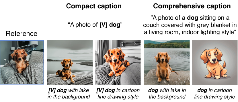
Figure 2: Comprehensive caption. We provide examples of compact caption (Ruiz et al., 2023a) and our comprehensive caption (top row) and generated images from each method (bottom row). The model fine-tuned with compact caption (left) generates images of a dog sitting on a couch though asked to be on the lake. Our comprehensive caption (right) effectively disentangles unwanted attributes, generating images that follow text prompts more faithfully.

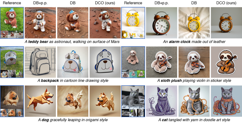
Figure 3: Custom subject generation. We show selected generations from DreamBooth (DB), DB with prior preservation (DB+p.p.), and ours (DCO) of custom subjects with varying attributes and styles guided by text prompts. While DB captures subjects well, it does not follow text prompt well. DB+p.p. shows better textual alignment, but falls short in subject fidelity. Ours show the best in both image-text alignment and subject fidelity. Best viewed in color, zoomed in on monitor.

4.3 Prompt Construction for Reference Images

Comprehensive caption. An important (yet often overlooked) part of the T2I personalization process is the prompt construction of reference images. Recall that Ruiz et al. (2023a) have proposed the use of a compact prompt in the form of “a photo of [V] [class]” with a rare token identifier [V]. However, we find that the use of compact caption is prone to learning distractors, such as a background or a style, as part of the fine-tuned model, as in Fig. 2.

Instead, we propose to provide a comprehensive and visually grounded caption that not only describes the subject but also details other visual attributes, backgrounds, and styles of reference images. In Fig. 2, we show an example of a comprehensive caption and compare the synthesized results that use a compact caption. We find that providing detailed descriptions of the undesirable attributes, e.g., background, or style, helps anchor desirable attributes in reference images to corresponding texts, making it easier to separate between them. This method not only holds for subject customization, but also for style customization; we provide comprehensive descriptions of the subject so that the model distinguishes style from the subject. Note that the use of comprehensive caption has been considered in practice, but has not been investigated from the lens of model shift and concept disentanglement. In our experiments, we use vision-language models such as GPT-4 (Achiam et al., 2023) or LLaVA (Liu et al., 2023) (e.g., see Fig. 11).

Learning textual embeddings.  The rare token identifier [V], such as “sks”, conveys undesirable semantics. Thus, we opt to remove the rare token identifier and use the natural language captions by default. In addition, we learn textual embeddings (Gal et al., 2022) to add more flexibility in subject personalization without changing the semantics of pretrained model. Given a word or a phrase (i.e., [class]) of interest, we insert new tokens and initialize them with textual embeddings of original ones. Then, newly inserted textual embeddings are optimized with diffusion models.

5 Experiments

We use Stable Diffusion XL (SDXL) (Podell et al., 2023) for the pretrained T2I diffusion model. We conduct experiments on subject (Sec. 5.1), style (Sec. 5.2) personalization, and their combination (Sec. 5.3). Ablative studies are in Sec. 5.4.

5.1 Subject Personalization

Experimental setup.  We conduct experiments on DreamBooth dataset (Ruiz et al., 2023a), containing 30 subjects, with 4–6 images per subject. The examples of images and captions are in Fig. 11 in Appendix D.1. To evaluate the effectiveness of DCO loss, we apply the same techniques (e.g., comprehensive caption, learning textual embedding) to baselines, though we omit indications of the use of these techniques when it is clear from the context. We present the efficacy of other techniques in Sec. 5.4 and Appendix B.1.

For baselines, we consider the model trained with a regular diffusion loss (DB) and the one with prior preservation loss (DB+p.p). For all experiments, we fine-tune LoRA of rank $32$ and textual embeddings using Adam (Kingma & Ba, 2014) optimizer with learning rates of 5e-5 and 5e-4, respectively. We use $\beta=1.0$ for DCO loss.

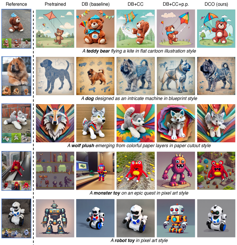
Figure 16: Custom subject generation. We compare our method (DCO) with pretrained model, and default DreamBooth (DB baseline with a compact caption), with comprehensive captions (DB+CC), with prior preservation loss (DB+CC+p.p.). Note that images in each row are generated using the same random seed. Our method is able to generate subject consistent images with various accessories, background or style, with better image-text alignment than baseline methods.

Qualitative results.  Fig. 3 shows the qualitative comparison of our approach with DreamBooth (DB) and DreamBooth using prior preservation loss (DB+p.p.). We observe that our approach can generate images of various visual attributes, e.g., outfits and backgrounds, or changing the material, as well as into various styles, e.g., in origami style or doodle art style. While DB changes the background, it lacks compositional generation in different outfits or styles, especially due to the overfitting to the photographic style. DB+p.p. does better than DB at compositional generation, but it often fails to preserve the subject identity (e.g., alarm clock, backpack, dog). More qualitative comparisons are demonstrated in Fig. 16.

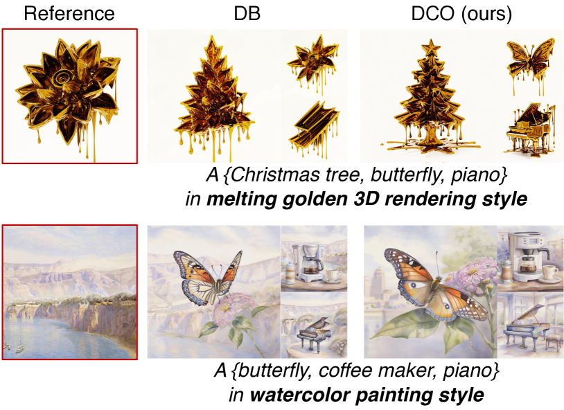
Figure 4: Custom style generation. We show selected generations from DreamBooth (DB) and ours (DCO) of custom styles with varying subjects. DB is prone to capturing undesirable attributes, resulting in generation of mixed concepts (e.g., butterfly mixed with the flower in the first row, background of mountain and sky appearing in the second row), whereas DCO mitigates such a concept mixing. Best viewed in color, zoomed in on monitor.

Quantitative results.  For quantitative evaluation, we design two types of text prompts: subject customization, where we modify the attributes of the subject or its background, and subject stylization, where we change the visual style of a subject image. For each subject and type, we generate images from 50 text prompts with 2 random seeds. For evaluation metrics, we report the image similarity score using DINOv2 (Oquab et al., 2023) and the image-text similarity score using SigLIP (Zhai et al., 2023). See Appendix D for details on evaluation prompts and metrics.

Noting that this is a multi-objective problem (i.e., maximizing image similarity and image-text similarity), we report the Pareto curve consisting of scores with varying reward guidance scale values to show the tradeoff between two scores of each model, instead of reporting scores at one operating point. If two curves overlap, two methods would likely perform similarly and the difference is up to a change in the reward guidance scale at sampling.

Averaged results are in Fig. 1, and results for each subject customization and stylization are in Fig. 9(a) and Fig. 9(b) in Appendix B.1, respectively. Compared to DreamBooth+CC (red), DCO+CC (blue) depicts the upper-right frontier in both image-text similarity and image similarity, demonstrating its effectiveness. Compared to DreamBooth with prior preservation loss (DreamBooth+CC+p.p.; green), ours (blue) results in significantly improved image similarity, while being comparable in image-text similarity. Interestingly, it (green) does not push the frontier to the upper-right compared to the ones without it (red), but it shifts the operating point to the lower-right while lying on the seemingly similar Pareto frontier. This suggests that the use of prior preservation loss improves prompt fidelity at the cost of losing the subject consistency. In Appendix B.1, we further demonstrate the effectiveness of DCO by comparing with various design choices for DreamBooth, such as early stopping or lowering $\lambda_{\textrm{prior}}$ values for prior preservation loss.

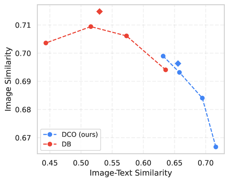
Figure 5: Quantitative results in style personalization. We plot image similarity and image-text similarity for style customization experiment for DreamBooth (DB) and DCO (ours). We plot the scores from reward guidance sampling (dots and dotted lines), and conventional classifier-free guidance sampling (diamond). See Sec. 5.2 for more details.

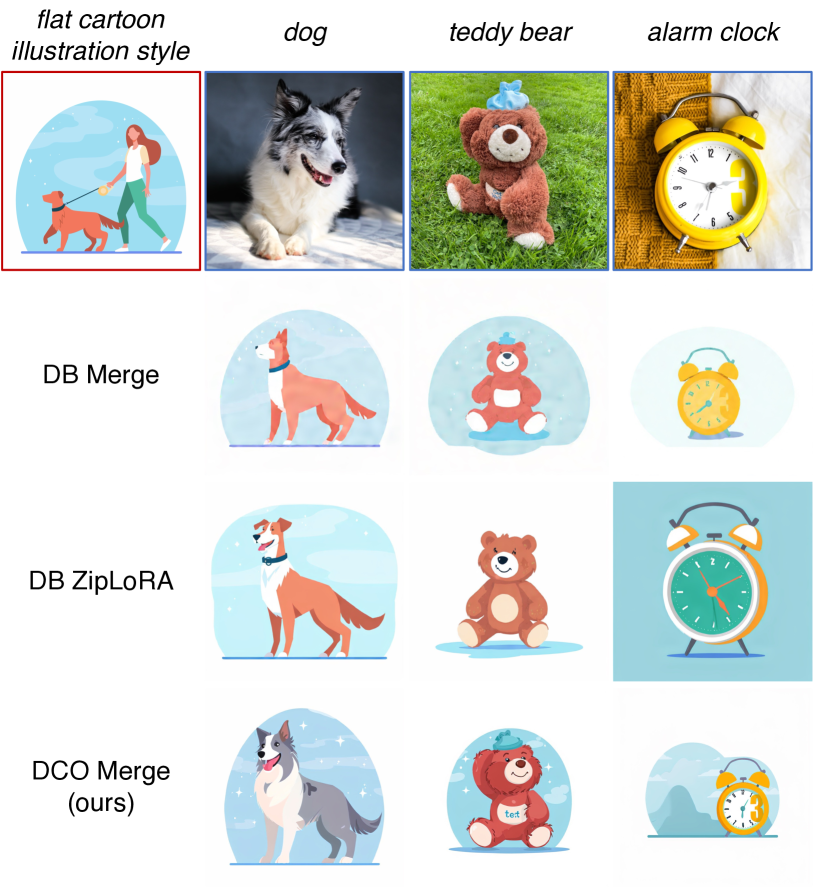
Figure 6: My subject in my style generation. We show images generated by merging subject and style LoRAs, each trained independently with DB (DB Merge) or DCO (DCO Merge). We also show results of ZipLoRA (Shah et al., 2023) from DB models. DB Merge struggles to generate high quality images composing subject and style. DB ZipLoRA improves the quality, but subject is less preserved. Our (DCO Merge) produces consistent images in both subject and style. Best viewed in color, zoomed in on monitor.

5.2 Style Personalization

Experimental setup.  We experiment on style images from StyleDrop dataset (Sohn et al., 2023). The examples of style images and captions are in Fig. 12 in Appendix D.1. We fine-tune LoRA of rank 64 using Adam optimizer with a learning rate of 5e-5 and do not train textual embedding. In addition, we add an offset noise (Guttenberg, 2023) of $0.1$ during training, which empirically helps learning the solid background color of style images. We use $\beta=1.0$ for DCO loss, and compare with DreamBooth (DB) as a baseline.

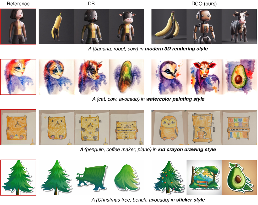
Figure 17: Custom style generation. Additional qualitative results on custom style generation. Our method (DCO) is able to generate style consistent image, while prior method, DreamBooth (DB), is prone to overfitting. For example, in the first row, the outfit and the pose of woman in reference image is inherited to banana, robot, and cow in DB, while our methods disentangle such attributes in generation. Those are also shown in second, third and fourth row.

Qualitative results.  Fig. 4 shows qualitative comparisons between DreamBooth (DB) and ours (DCO). As seen in (Shah et al., 2023), DB captures the style of a reference image, yet it suffers from overfitting to the reference image, e.g., the attributes of the subject in style reference appear in generated images. On the other hand, DCO generates images with consistent style without being entangled with subjects (e.g., flower, cliffs, and sky) in the reference images. We provide additional comparisons in Fig. 17 in Appendix.

Quantitative results.  We choose 10 style images and generate stylized images using 190 text prompts excerpted from Parti prompts (Yu et al., 2022), following (Sohn et al., 2023). We generate 2 images per evaluation prompt, resulting in 380 images in total for each style. For evaluation metrics, we report the image similarity against the style reference image and image-text similarity scores using SigLIP (Zhai et al., 2023). Similarly to Sec. 5.1, we report scores using reward guidance sampling with $\omega_{\textrm{rg}}\in\{2.0,3.0,4.0,5.0\}$.

Fig. 5 shows results. While two models operate in somewhat disjoint regimes, we see that the curve of DCO (ours) is placed on the right of that of DB, showing improved image-text similarity. Nevertheless, as noted in (Sohn et al., 2023), the image similarity for style personalization is particularly noisy, as the score is not only guided by the style but also by the unexpected appearance of the subject in the style reference image (e.g., in Fig. 4) when the model overfits.

5.3 My Subject in My Style

Experimental setup.  Following (Sohn et al., 2023), we combine customized subject and style models to generate images of my subject in my style. Specifically, given two LoRAs $\Delta W_{1}$ and $\Delta W_{2}$ for subject and style, respectively, we use an arithmetic merge (Merge) (Shah et al., 2023), i.e., $\Delta W=\lambda_{1}\Delta W_{1}+\lambda_{2}\Delta W_{2}$ with coefficients $\lambda_{1}$ and $\lambda_{2}$. We use subject and style LoRAs from Sec. 5.1 and Sec. 5.2, respectively, for both baseline (DB) and our method (DCO). We also compare with ZipLoRA (Shah et al., 2023), which finds optimal coefficients $\lambda_{1}$ and $\lambda_{2}$ that preserve identities of each subject and style personalized model while minimizing their interference. For ZipLoRA, we use DreamBooth fine-tuned subject and style models and follow the experimental setup in (Shah et al., 2023). We do not use reward guidance sampling for either method.

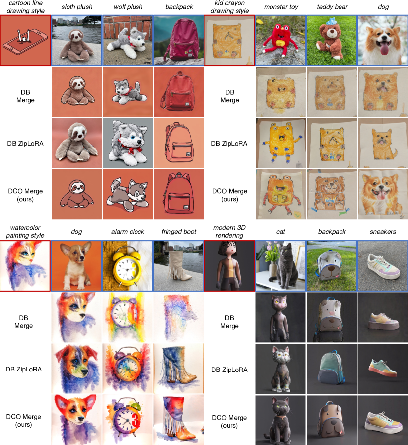
Figure 18: My subject in my style generation. Additional results are shown. Our method (DCO Merge) generates an image that maintains subject and style consistency without any post-processing. On the other hand, DreamBooth Merge (DB Merge) shows inferior results as is either overfitted to subject (e.g., sloth plush, wolf plush, backpack are not in cartoon line drawing style), or styles (e.g., monster toy, teddy bear, dog do not appear in kid crayon drawing style). Meanwhile, ZipLoRA shows better results than DB Merge, yet it often loses the subject or style fidelity.

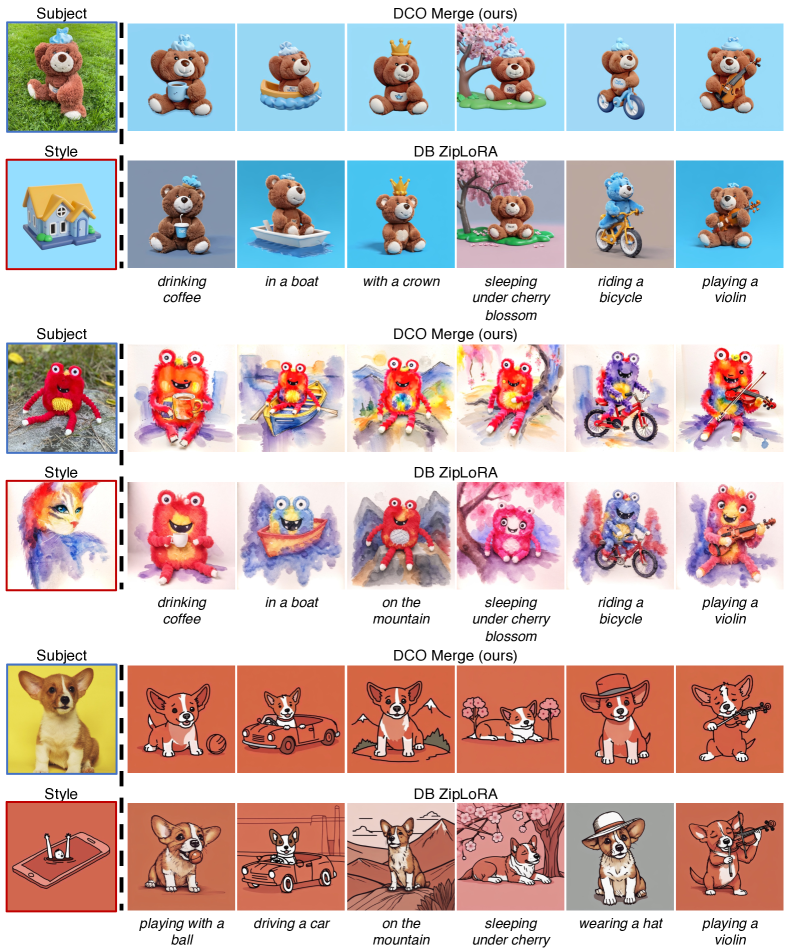
Figure 19: Text-compositional my subject in my style generation. We show more qualitative results for my subject in my style generation that compare arithmetic merge of DCO fine-tuned models (DCO Merge) and ZipLoRA (Shah et al., 2023) on DB fine-tuned models. DCO Merge generates images consistent to both subject and style without further post-optimization, while ZipLoRA often misses the subject or style consistency (e.g., teddy bear and monster toy are changed, and the style of the third example is not as consistent).

Qualitative results.  In Fig. 6, we provide qualitative comparisons between our approach (DCO Merge), and baselines (DB Merge and DB ZipLoRA). As noticed in (Shah et al., 2023), DB Merge struggles to generate high-quality images when composing subject and style customized models. While DB ZipLoRA improves the image quality with fewer artifacts, it loses subject or style consistency after post-processing. Even using a simple arithmetic merge, DCO Merge (ours) generates images with high subject and style consistency. Furthermore, as in Fig. 7, DCO Merge generates custom subjects in custom style under various contexts, guided by text prompts. See Fig. 18 and Fig. 19 for more qualitative comparisons.

Quantitative results.  We use 30 subjects from DreamBooth (Ruiz et al., 2023a) dataset and 10 style images from StyleDrop dataset (Sohn et al., 2023) from Sec. 5.1 and Sec. 5.2, respectively. For each subject and style pair, we generate images of “A [subject] in [style]” and of various text prompts that change attributes, backgrounds, or actions (e.g., in Fig. 7). We compute subject similarity scores using DINO v2 (Oquab et al., 2023), style similarity, and image-text similarity scores using SigLIP (Zhai et al., 2023).

Tab. 1 reports quantitative results. DCO Merge significantly outperforms DB Merge and DB ZipLoRA in subject similarity ($0.462$ vs. $0.386$, $0.406$) and image-text similarity ($0.773$ vs. $0.430$, $0.729$), while retaining competitive style similarity ($0.651$ vs. $0.672$, $0.662$). This is aligned with our observation in Fig. 6 and Fig. 7.

Why does it work?  DCO Merge enjoys the computational efficiency over ZipLoRA (Shah et al., 2023), enabling the composition of customized subject and style models for free. On the other hand, this naturally raises the question of why DCO-trained LoRAs can be combined. We attribute it to the training mechanism of DCO, where models are fine-tuned while retaining the consistency to the pretrained model. As such, two fine-tuned models, each of which is trained to be consistent with the pretrained model, are more likely to be consistent with each other than models trained with DB. We study this more in-depth in Sec. 5.4 and Fig. 8(c).

Table 1: Quantitative results of my subject in my style generation. We report subject, style, and image-text similarity scores of arithmetic merge of DB subject and style models (DB Merge), ZipLoRA of DB models (DB ZipLoRA), and arithmetic merge of DCO models (DCO Merge).

	DB Merge	DB ZipLoRA	DCO Merge
Subject Similarity	0.386	0.406	0.462
Style Similarity	0.672	0.662	0.651
Image-Text Similarity	0.430	0.729	0.773

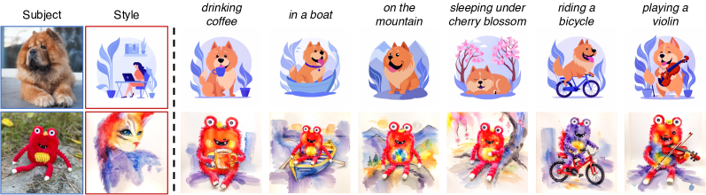
Figure 7: Compositional generation of my subject in my style. We show generated examples of my subject in my style with various actions or visual attributes given by text prompts. We merge independently trained subject and style personalized models with our method (i.e., DCO Merge). Best viewed in color, zoomed in on monitor.

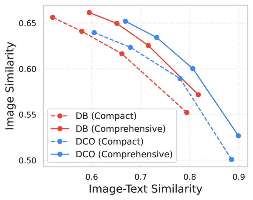
(a) Ablation on comprehensive caption

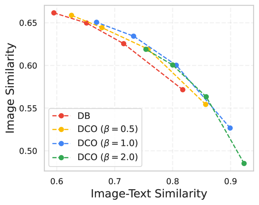
(b) Ablation on $\beta$

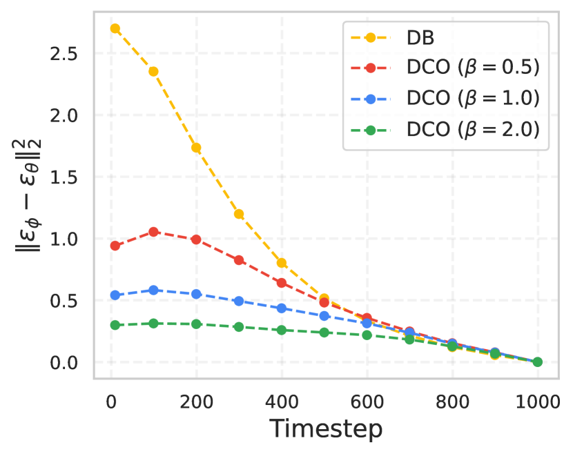
(c) Noise distance

Figure 8: Ablation studies. We conduct ablation studies on (a) comprehensive caption, (b) $\beta$, and (c) noise distance between pretrained model and fine-tuned model.

5.4 Ablation Study

Comprehensive caption. We study the effect of comprehensive caption. We select 10 subjects from DreamBooth dataset and compare with compact captions on both DreamBooth (DB) and DCO, using the same experimental setup as in Sec. 5.1. Fig. 8(a) shows the Pareto curves with reward guidance of varying scales. We observe that comprehensive caption (solid line) forms an upper-right frontier compared to compact caption (dashed line) for both DB and DCO.

Regularization parameter $\mathbf{\beta}$.  We study the effect of the regularization parameter $\beta$ on the subject personalization task. We use 10 subjects from the DreamBooth dataset and conduct experiments with $\beta=\{0.5,1.0,2.0\}$. As in Fig 8(b), all DCO models form a better Pareto frontier than the DB from Sec. 5.1. As $\beta$ becomes larger the curve tends to move lower right, implying the loss in subject identity for better image-text alignment. This is expected as $\beta$ controls the KL divergence between fine-tuned and pretrained models (e.g., Eq. (5)). We find $\beta\,{=}\,1.0$ works well overall, though the optimal $\beta$ might vary across the reference dataset.

Error analysis.  One of our insights is that DCO mitigates the shift in the model’s generation distribution after fine-tuning. We verify this by computing the noise distance between pretrained and fine-tuned models on reference images and prompts, i.e., $\|\boldsymbol{\varepsilon}_{\theta}(\mathbf{x}_{t};\mathbf{c},t)-\boldsymbol{\varepsilon}_{\phi}(\mathbf{x}_{t};\mathbf{c},t)\|_{2}^{2}$ at each timestep $t\,{\in}\,[0,1000]$. We simulate 100 random noises at each timestep and report the average value in Fig. 8(c). We see a clear decrease in noise deviation from the pretrained model with DCO fine-tuning over DB. Moreover, as $\beta$ increases, the noise deviation gets further reduced as expected.

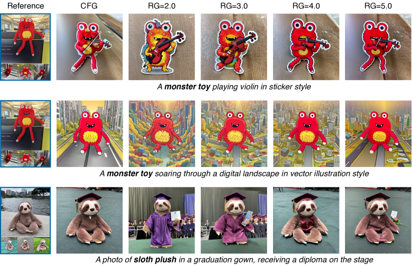
Figure 13: Effect of reward guidance scale. We show the effect of reward guidance (RG) scale by varying from 2.0 to 5.0. We also show the synthesized results using CFG. Note that the optimal choice of reward guidance scale (in consideration of user’s preference) might varies among reference dataset, or even input prompts.

Effect of reward guidance.  Our quantitative results (e.g., Fig. 1, Fig. 8(b)) show that reward guidance sampling controls the textual alignment and subject fidelity, which gives the control over these two axes. Yet, an optimal guidance scale may vary across the reference dataset as well as the input prompt. We provide qualitative examples in Fig. 13.

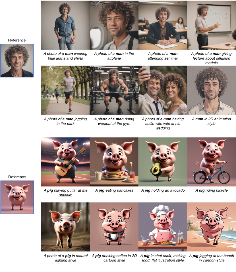
Figure 14: 1–shot personalization using synthetic images generatd by SDXL. We show the capability of our method in 1–shot subject personalization using the images generated by pretrained SDXL models. For each reference image (man and pig), DCO fine-tuned T2I models can generate subjects with different actions and styles. The prompts that used to generate reference images were “a photo of a 50 years old man with curly hair” and “a 3D animation of happy pig”, respectively, as used in (Avrahami et al., 2023).

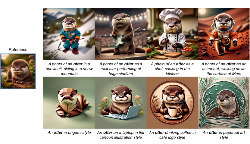
Figure 15: 1–shot personalization using synthethic images generated by DALLE-3. We show the capability of our method in 1–shot subject personalization using the images generated by DALLE–3 (Betker et al., 2023). We asked ChatGPT to generate a cute baby otter image. The comprehensive caption to fine-tune this image is “A closed-up photo of an <otter> on the top of wooden log, forest in the background". Our method is able to recontextualize the subject in the reference image with various text prompts depicting accessories, background, or style.

1–shot personalization.  Finally, we showcase the 1–shot personalized image synthesis results of our method. We refer to Appendix B.3 for experimental details and qualitative results are in Fig. 14 and Fig. 15.

6 Conclusion

We introduce a recipe for low-shot fine-tuning of the T2I diffusion model. This includes Direct Consistency Optimization (DCO), a novel fine-tuning objective that promotes the consistency of the model to the pretrained model, thus enhancing the compositionality of personalized T2I models. We show the necessity of comprehensive captions and propose a reward guidance sampling scheme that balances the subject fidelity and text prompt fidelity trade-off. T2I diffusion models fine-tuned via DCO outperform previous baselines in learning subjects and styles, resulting in a superior Pareto frontier. Moreover, our approach enables the composition of independently fine-tuned subject and style T2I models without further post-processing.

Impact Statements

This paper presents a method that enhances the performance of the personalization of T2I diffusion models. Similarly to other works, the technology for personalization of T2I diffusion models comes with benefits and pitfalls – the tool could be extremely effective for creative directors to efficiently generate new visual assets of various subjects or styles derived from existing private visual assets. Yet, the responsible use of the technology is required for protecting the ownership and copyright of individual assets.

Appendix A Derivation of Direct Consistency Optimization (DCO) loss

Given a consistency reward $r(\mathbf{x},\mathbf{c})$, our goal is to solve following:

$$\max_{\theta}~{}\mathbb{E}_{\mathbf{c},\mathbf{x}_{0}\sim p_{\theta}(\mathbf{x}_{0}|\mathbf{c})}[r(\mathbf{x}_{0},\mathbf{c})]-\beta D_{\textrm{KL}}\big{(}p_{\theta}(\cdot|\mathbf{c})\,\|\,p_{\phi}(\cdot|\mathbf{c})\big{)}\text{,}$$ (14)

where $p_{\phi}(\cdot|\mathbf{c})$ is a distribution of pretrained diffusion model. Since the distribution $p_{\theta}$ (nor $p_{\phi}$) is intractable (as the diffusion models takes non-parametrized inference), we instead consider the marginalization over all diffusion trajectories $\mathbf{x}_{0:T}$. We define the reward on the diffusion path and define the reward to be the expectation over all reverse processes, i.e., let $\hat{r}(\mathbf{x}_{0:T},\mathbf{c})$ be reward on a single diffusion path, then the total reward on $(\mathbf{x}_{0},\mathbf{c})$ is given as

$$r(\mathbf{x}_{0},\mathbf{c})=\mathbb{E}_{\mathbf{x}_{1:T}\sim p_{\theta}(\mathbf{x}_{1:T}|\mathbf{x}_{0},\mathbf{c})}[\hat{r}(\mathbf{x}_{0:T},\mathbf{c})]\text{.}$$ (15)

Then using the variational upper bound on the KL divergence in Eq. (1), we derive following lower bound for the objective in Eq. (14):

$$\max_{\theta}~{}\mathbb{E}_{\mathbf{c},\mathbf{x}_{0}\sim p_{\theta}(\mathbf{x}_{0}|\mathbf{c})}[r(\mathbf{x}_{0},\mathbf{c})]-\beta D_{\textrm{KL}}\big{(}p_{\theta}(\cdot|\mathbf{c})\|p_{\phi}(\cdot|\mathbf{c})\big{)}$$ (16)

$$\geq \max_{\theta}~{}\mathbb{E}_{\mathbf{c},\mathbf{x}_{0:T}\sim p_{\theta}(\mathbf{x}_{0:T}|\mathbf{c})}[\hat{r}(\mathbf{x}_{0:T},\mathbf{c})]-\beta D_{\textrm{KL}}\big{(}p_{\theta}(\mathbf{x}_{0:T}|\mathbf{c})\|p_{\phi}(\mathbf{x}_{0:T}|\mathbf{c})\big{)}\text{.}$$ (17)

It is well-known that Eq. (17) has a closed-form solution given as follows:

$$p_{\theta^{\ast}}(\mathbf{x}_{0:T}|\mathbf{c})=p_{\phi}(\mathbf{x}_{0:T}|\mathbf{c})\exp\big{(}\hat{r}(\mathbf{x}_{0:T},\mathbf{c})/\beta\big{)}/Z(\mathbf{c})\text{,}$$ (18)

where $Z(\mathbf{c})\,{=}\,\mathbb{E}_{p_{\phi}(\mathbf{x}_{0:T},\mathbf{c})}\big{[}\exp\big{(}\hat{r}(\mathbf{x}_{0:T}|\mathbf{c})/\beta\big{)}\big{]}$ is a normalization constant that does not depend on $\theta$ of the fine-tuned model. Similarly to DPO (Rafailov et al., 2023; Wallace et al., 2023), we are interested in devising the training objective by using implicitly defined reward function, which is given as follows:

$$\hat{r}(\mathbf{x}_{0:T},\mathbf{c})=\beta\log\frac{p_{\theta}(\mathbf{x}_{0:T}|\mathbf{c})}{p_{\phi}(\mathbf{x}_{0:T}|\mathbf{c})}+\beta\log Z(\mathbf{c})\text{,}$$ (19)

and the total reward $r(\mathbf{x},\mathbf{c})$ becomes

$$r(\mathbf{x}_{0},\mathbf{c})=\mathbb{E}_{\mathbf{x}_{1:T}\sim p_{\theta}(\mathbf{x}_{1:T}|\mathbf{x}_{0},\mathbf{c})}\bigg{[}\beta\log\frac{p_{\theta}(\mathbf{x}_{0:T}|\mathbf{c})}{p_{\phi}(\mathbf{x}_{0:T}|\mathbf{c})}\bigg{]}+\beta\log Z(\mathbf{c})\text{.}$$ (20)

Since our goal is to fine-tune the model by shifting as small as possible from the pretrained model, we devise the training objective by comparing the induced reward using fine-tuning model $p_{\theta}$ and using the pretrained model $p_{\phi}$. To be specific, given $(\mathbf{x}_{0},\mathbf{c})\sim\mathcal{D}_{\textrm{ref}}$ a data pair sampled from reference dataset, and consider diffusion trajectories $\mathbf{x}_{1:T}\sim p_{\theta}(\mathbf{x}_{1:T}|\mathbf{x}_{0},\mathbf{c})$ and $\mathbf{x}_{1:T}^{\prime}\sim p_{\phi}(\mathbf{x}_{1:T}^{\prime}|\mathbf{x}_{0},\mathbf{c})$. Then we enforce the total reward $r(\mathbf{x}_{0},\mathbf{c})$ to be larger than the expectation of $\hat{r}(\mathbf{x}_{0:T}^{\prime},\mathbf{c})$ over the distribution of diffusion paths $p_{\phi}(\mathbf{x}_{1:T}|\mathbf{x}_{0},\mathbf{c})$. Formally, this can be written as

$$\begin{split}r(\mathbf{x}_{0},\mathbf{c})=&\mathbb{E}_{\mathbf{x}_{1:T}\sim p_{\theta}(\mathbf{x}_{1:T}|\mathbf{x}_{0},\mathbf{c})}[\hat{r}(\mathbf{x}_{0:T},\mathbf{c})]>\mathbb{E}_{\mathbf{x}_{1:T}^{\prime}\sim p_{\phi}(\mathbf{x}_{1:T}^{\prime}|\mathbf{x}_{0},\mathbf{c})}[\hat{r}(\mathbf{x}_{0:T}^{\prime},\mathbf{c})]\text{.}\end{split}$$ (21)

At high level, for any diffusion path that has $\mathbf{x}$ at $t=0$, the total reward should be greater than the marginalization over the pretrained distribution. This is in contrast to the DPO (Rafailov et al., 2023; Wallace et al., 2023), where they perform contrastive objective between data pair; they enforce the total reward of preferred one to be larger than non-preferred one.

Yet, it is still challenging to compute the expectation in RHS of Eq. (21). To this end, we derive its upper bound and provide a tighter condition for $r(\mathbf{x},\mathbf{c})$. Remark that we have

$$\mathbb{E}_{p_{\phi}(\mathbf{x}_{1:T}^{\prime}|\mathbf{x}_{0},\mathbf{c})}[\hat{r}(\mathbf{x}_{0:T}^{\prime},\mathbf{c})] =\mathbb{E}_{p_{\phi}(\mathbf{x}_{1:T}^{\prime}|\mathbf{x}_{0},\mathbf{c})}\bigg{[}\beta\log\frac{p_{\theta}(\mathbf{x}_{0:T}^{\prime}|\mathbf{c})}{p_{\phi}(\mathbf{x}_{0:T}^{\prime}|\mathbf{c})}\bigg{]}+\beta\log Z(\mathbf{c})$$ (22)

$$=-\beta D_{\textrm{KL}}\big{(}p_{\theta}(\mathbf{x}_{0:T}^{\prime}|\mathbf{c})\|p_{\phi}(\mathbf{x}_{0:T}^{\prime}|\mathbf{c})\big{)}+\beta\log Z(\mathbf{c})$$ (23)

$$\leq\beta\log Z(\mathbf{c})\text{,}$$ (24)

where the last inequality comes from the non-negativity of KL divergence. From Eq. (24), we have tighter lower bound for the total reward as follows:

$$r(\mathbf{x}_{0},\mathbf{c})>\beta\log Z(\mathbf{c})\Leftrightarrow\mathbb{E}_{p_{\theta}(\mathbf{x}_{1:T}|\mathbf{x}_{0},\mathbf{c})}\bigg{[}\beta\log\frac{p_{\theta}(\mathbf{x}_{0:T}|\mathbf{c})}{p_{\phi}(\mathbf{x}_{0:T}|\mathbf{c})}\bigg{]}>0\text{.}$$ (25)

We simply shift the reward function with $\beta\log Z(\mathbf{c})$, and let $\hat{r}(\mathbf{x},\mathbf{c})=\beta\log\frac{p_{\theta}(\mathbf{x}_{0:T}|\mathbf{c})}{p_{\phi}(\mathbf{x}_{0:T}|\mathbf{c})}$. Then we use the logistic loss to fine-tune model to satisfy Eq. (25):

$$\min_{\theta}~{}\mathbb{E}_{(\mathbf{x}_{0},\mathbf{c})\sim\mathcal{D}_{\textrm{ref}}}\big{[}-\log\sigma(r(\mathbf{x}_{0},\mathbf{c}))\big{]}=\mathbb{E}_{(\mathbf{x}_{0},\mathbf{c})\sim\mathcal{D}_{\textrm{ref}}}\bigg{[}-\log\sigma\bigg{(}\mathbb{E}_{p_{\theta}(\mathbf{x}_{1:T}|\mathbf{x}_{0},\mathbf{c})}\bigg{[}\beta\log\frac{p_{\theta}(\mathbf{x}_{0:T}|\mathbf{c})}{p_{\phi}(\mathbf{x}_{0:T}|\mathbf{c})}\bigg{]}\bigg{)}\bigg{]}\text{,}$$ (26)

where $\sigma(u)=\frac{1}{1+\exp(-u)}$ is a sigmoid function.

However, it is challenging to optimize Eq. (26) as the joint distribution $p_{\theta}(\mathbf{x}_{0:T}|\mathbf{c})$ is intractable. Instead, we derive a variational upper bound to Eq. (26) for efficient implementation. First, since sampling from $\mathbf{x}_{1:T}\sim p_{\theta}(\mathbf{x}_{1:T}|\mathbf{x}_{0},\mathbf{c})$ is intractable, we instead marginalize the reward using the diffusion forward process, i.e., $q(\mathbf{x}_{1:T}|\mathbf{x}_{0})$. Then, the reward can be approximated as follows:

$$r(\mathbf{x}_{0},\mathbf{c})/\beta \approx\mathbb{E}_{q(\mathbf{x}_{1:T}|\mathbf{x}_{0})}\bigg{[}\log\frac{p_{\theta}(\mathbf{x}_{0:T}|\mathbf{c})}{p_{\phi}(\mathbf{x}_{0:T}|\mathbf{c})}\bigg{]}$$ (27)

$$=\mathbb{E}_{q(\mathbf{x}_{1:T}|\mathbf{x}_{0})}\bigg{[}\sum_{t=1}^{T}\log\frac{p_{\theta}(\mathbf{x}_{t-1}|\mathbf{x}_{t},\mathbf{c})}{p_{\phi}(\mathbf{x}_{t-1}|\mathbf{x}_{t},\mathbf{c})}\bigg{]}$$ (28)

$$=\mathbb{E}_{q(\mathbf{x}_{1:T}|\mathbf{x}_{0})}\bigg{[}\sum_{t=1}^{T}\log\frac{p_{\theta}(\mathbf{x}_{t-1}|\mathbf{x}_{t},\mathbf{c})}{q(\mathbf{x}_{t-1}|\mathbf{x}_{t},\mathbf{x}_{0})}-\sum_{t=1}^{T}\log\frac{p_{\phi}(\mathbf{x}_{t-1}|\mathbf{x}_{t},\mathbf{c})}{q(\mathbf{x}_{t-1}|\mathbf{x}_{t},\mathbf{x}_{0})}\bigg{]}$$ (29)

$$=\sum_{t=1}^{T}\mathbb{E}_{q(\mathbf{x}_{t}|\mathbf{x}_{0})}\big{[}-D_{\textrm{KL}}(q(\mathbf{x}_{t}|\mathbf{x}_{t-1},\mathbf{x}_{0})\|p_{\theta}(\mathbf{x}_{t-1}|\mathbf{x}_{t},\mathbf{c}))+D_{\textrm{KL}}(q(\mathbf{x}_{t}|\mathbf{x}_{t-1},\mathbf{x}_{0})\|p_{\phi}(\mathbf{x}_{t-1}|\mathbf{x}_{t},\mathbf{c}))\big{]}$$ (30)

$$=\mathbb{E}_{\boldsymbol{\varepsilon}\sim\mathcal{N}(\boldsymbol{0},\mathbf{I}),t\sim\mathcal{U}[1,T]}\big{[}-T\omega(t)\big{(}\|\boldsymbol{\varepsilon}_{\theta}(\mathbf{x}_{t};\mathbf{c},t)-\boldsymbol{\varepsilon}\|_{2}^{2}-\|\boldsymbol{\varepsilon}_{\phi}(\mathbf{x}_{t};\mathbf{c},t)-\boldsymbol{\varepsilon}\|_{2}^{2}\big{)}\big{]}\text{,}$$ (31)

where Eq. (31) is from variational lower bound of diffusion loss (Kingma et al., 2021). Then from Jensen’s inequality, we have our DCO loss given as follows:

$$\mathcal{L}_{\textrm{DCO}}(\theta)\coloneqq\mathbb{E}_{(\mathbf{x},\mathbf{c})\sim\mathcal{D}_{\textrm{ref}},t\sim\mathcal{U}(0,T),\boldsymbol{\varepsilon}\sim\mathcal{N}(\boldsymbol{0},\mathbf{I})}\big{[}-\log\sigma\big{(}-\beta T\omega(t)(\|\boldsymbol{\varepsilon}_{\theta}(\mathbf{x}_{t};\mathbf{c},t)-\boldsymbol{\varepsilon}\|_{2}^{2}-\|\boldsymbol{\varepsilon}_{\phi}(\mathbf{x}_{t};\mathbf{c},t)-\boldsymbol{\varepsilon}\|_{2}^{2})\big{)}\big{]}\text{.}$$ (32)

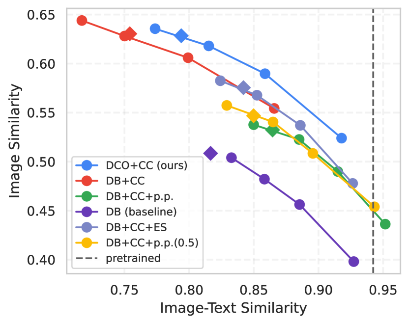
(a) Subject Customization

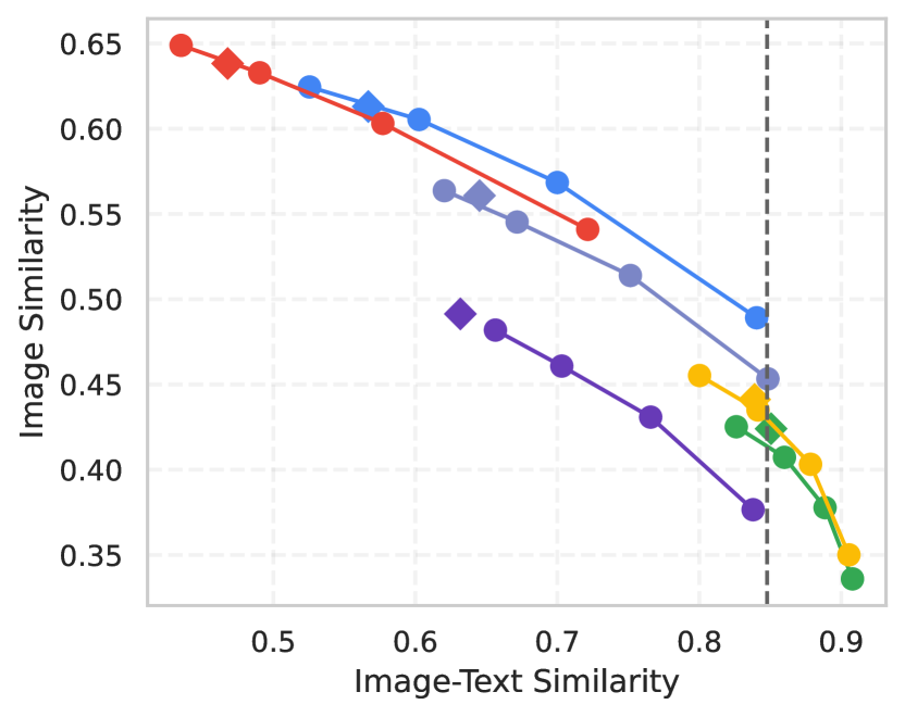
(b) Subject Stylization

Figure 9: Quantitative results. We plot image similarity and image-text similarity for each (a) subject customization and (b) subject stylization experiment. We use SigLIP (Zhai et al., 2023) score for image-text similarity, and DINO (Oquab et al., 2023) score for image similarity. We plot the results of reward guidance sampling (dots and solid lines), and conventional sampling (diamond). The reported reward guidance scales are $\omega_{\textrm{rg}}\in\{2.0,3.0,4.0,5.0\}$.

Appendix B Additional Experiments

B.1 Full comparison

Here we provide full ablation studies that we have conducted in our experiments. For all 30 subjects in DreamBooth dataset, we follow the same experimental setup as in Sec. 5.1. We report the image similarity score using DINOv2 (Oquab et al., 2023), and image-text similarity score using SigLIP (Zhai et al., 2023).

Ablation on early stopping.

Since low-shot fine-tuning methods suffer from overfitting, it is a common practice to early stop the training. In Fig. 9(b) and Fig. 9(b), we plot the results of DreamBooth with comprehensive caption with half of training steps (DB+CC+ES). When compared to DB+CC, it improves the image-text similarity ($0.842$ vs. $0.754$ for customization, $0.645$ vs. $0.468$ for stylization), while the image similarity significantly drops ($0.575$ vs. $0.754$ for customization, $0.630$ vs. $0.638$ for stylization). Notably, we remark that the frontier curve of DB+CC+ES resides at the frontier of DB+CC. Thus, early stopping does not improve the frontier.

Ablation on prior preservation loss weight $\lambda_{\textrm{prior}}$.

In Sec. 5.1, we show that using prior preservation loss often leads to loss of subject consistency. To further verify the effect of prior preservation loss, we vary the coefficient $\lambda_{\textrm{prior}}$ to be $0.5$ (DB+CC+p.p. (0.5)). As shown in Fig. 9(a) and Fig. 9(b), when compare to DB+CC+p.p., using smaller $\lambda_{\textrm{prior}}$ improves image similarity ($0.547$ vs. $0.532$ for customization, $0.441$ vs. $0.424$ for stylization), while decreases the image-text similarity (0.850 vs. 0.864 for customization, $0.839$ vs. $0.851$ for stylization). However, changing $\lambda_{\textrm{prior}}$ does not improve the frontier curve when using reward guidance.

Prior preservation loss vs. pretrained model.

In Fig. 9(a) and Fig. 9(b), we notice that DB with prior preservation loss (DB+CC+p.p.) shows higher image-text similarity than pretrained model. This is in partly due to that the model is fine-tuned with class-specific prior dataset, which improves the prompt fidelity among the class. However, this does not necessarily improves the subject fidelity, and it indicates the large model shift with respect to pretrained model.

Qualitative comparisons.

We further compare the baselines by providing qualitative examples in Fig. 16. As we observed in our quantitative analysis, the methods within DB+CC generally overfits, struggles in generating the subject in different styles. On the other hand, DB+CC+p.p. generally underfits to the subject, which might generate the image that follows prompt, but struggles in preserving the subject consistency. Also, using rare token identifier often generates infavorable results, such as weapons, as we mentioned in Sec. 4.3.

B.2 Effect of Reward Guidance Scale.

We have shown that the user can control the subject fidelity and textual alignment by changing the reward guidance scale. Yet, we remark that the optimal reward guidance scale vary among the reference dataset, and even for the input prompt that the user give during inference. As shown in Fig. 13, the optimal guidance scale should be large (e.g., $5.0$) for the first row, while it should be low (e.g., $2.0$) for the third row. Also, the effect of reward guidance scale might be subtle as in second row. In practice, choosing the best reward guidance scale is up to the user’s preference.

B.3 1-shot personalization

Here we provide some qualitative examples that shows the capability of our method in learning subjects with single reference image. Specifically, we show the capability of personalization with synthetic images, generated by different T2I models such as pretrained SDXL (Podell et al., 2023) and DALLE–3 (Betker et al., 2023). We follow the same setup as in Sec. 5.1 except that we fine-tune for 1000 steps. Remark that for while we have access to the prompts that we used for generation, we did not use this prompt for fine-tuning our model; the generated image might have more details (e.g., backgrounds or attributes), or it may fail to capture all the prompts. Thus, we caption the images following Sec. 4.3.

Fig. 14 shows the qualitative results of DCO fine-tuning on images generated by SDXL. Remark that our method can synthesize images into various actions and styles, while preserving the subject consistency. Notably, it is possible to convert the photographs to other styles (e.g., photo of a man to 2D animation style), and vice versa (e.g., 3D animation style of pig into photography). Also, as shown in Fig. 15, our method is able to generate various actions, backgrounds, or styles.

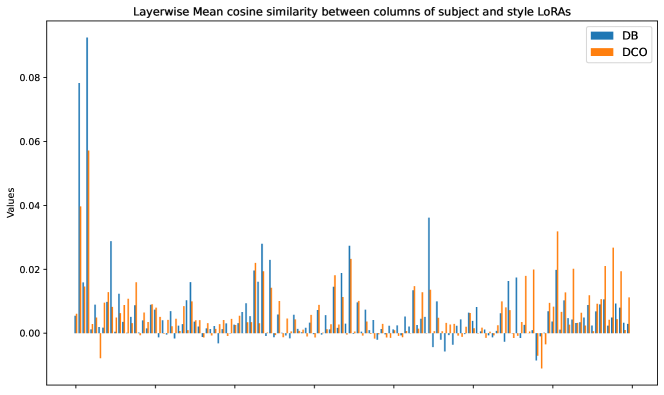
Figure 10: Comparison on the alignment of DreamBooth and DCO fine-tuned subject and style LoRAs. We compute the average cosine similarity of column layers between subject and style LoRAs fine-tuned with each DreamBooth (DB) (Ruiz et al., 2023a) and our method (DCO). The x-axis denotes the component of each U-Net layer. The cosine similarity measures the alignment between two LoRAs, and high cosine similarity values are considered as the interference between them. Interestingly, we find that there is no obvious difference in the cosine similarity values between models trained with DCO and DB methods, while DCO fine-tuned models can be successfully combined with arithmetic merge to generate images of my subject in my style (e.g., see Fig. 6 and Fig. 18). This may be in contrast with the findings of recent works (Shah et al., 2023; Po et al., 2023) and suggests further investigation on method to measure the compatibility between LoRA models.

Appendix C Extended Related Work

Training-free consistent image set generation.

Several works have demonstrated the capability of consistent image set generation without fine-tuning T2I diffusion models (Hertz et al., 2023; Tewel et al., 2024). While these methods do not require fine-tuning and hence may be conceived more time-saving, they often take longer time at generation. On the other hand, fine-tuning is a one-time cost and can be used for generation without additional cost. Also, training-free methods have difficulty in putting the same subject in different styles (as mentioned as limitation in (Tewel et al., 2024)), while our approach is possible. Moreover, our method is able to combine style personalized model and subject personalized model. Lastly, our approach do not require any segmentation mask for subject personalization.

Multi-concept personalization.

Given multiple fine-tuned T2I diffusion models (often using LoRAs), it is of great interest to combine them to generate a scene consists of multiple personalized subjects (Gu et al., 2023; Po et al., 2023), or generating custom subject in custom style (Sohn et al., 2023; Shah et al., 2023). Those approaches often require post-optimization, e.g., orthogonal adaptation of LoRA layers (Po et al., 2023) or optimization of merger coefficients for composition of subject and style LoRAs (Shah et al., 2023). Those methods hypothesize that the interference between subject and style LoRAs (which is measured by the average cosine similarity between LoRA layers), and aim to minimize the interference. Our method seeks for a better training of LoRA for T2I diffusion models and thus complementary to existing works. On the other hand, as shown in Fig. 10, we find that the cosine similarity values of DCO fine-tuned models are not necessarily smaller than those of DreamBooth fine-tuned models, while we do not observe significant interference during generation with arithmetically merged LoRAs trained with our DCO loss. This observation may suggest that we need another metric other than the cosine similarity based interference measure to evaluate the compatibility of LoRAs, which we leave as a future work.

Appendix D Experimental detail

D.1 Dataset

We use DreamBooth dataset (Ruiz et al., 2023a) for subject personalization which contains 30 subjects, including pets and unique objects such as backpack, dogs, plushie, etc. We provide examples of image and comprehensive caption in Fig. 11 where the complete list of comprehensive captions are is available in the source code. A comprehensive caption encompasses not only the subject but also provides detailed information on visual attributes, backgrounds, and style. In contrast, a compact caption generally incorporated in model personalization (Ruiz et al., 2023a; Gal et al., 2022) focuses solely on the subject itself, as exemplified by “a photo of [class]”. To generate comprehensive captions in practical scenarios, we initially employ LLaVA (Liu et al., 2023) to generate a description of the reference image. Subsequently, we filter out unnecessary details such as non-visual attributes and make further modifications. Similarily, we use 10 images from StyleDrop dataset (Sohn et al., 2023) for style personalization, where examples are presented in Fig. 12. Note that one can use different approach for the construction of comprehensive captions, e.g., utilizing different vision language model.

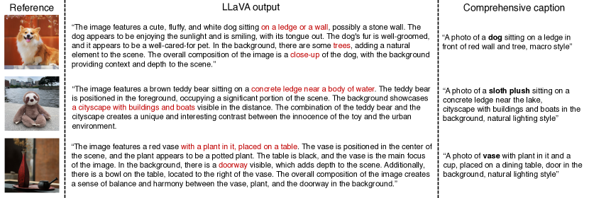
Figure 11: Examples of comprehensive caption for subject images. We provide examples of LLaVA (Liu et al., 2023) output and our comprehensive captions for each reference image. With help of LLaVA, we extract the visual attributes, backgrounds, and styles to construct comprehensive caption (e.g., the texts marked in red in LLaVA output are used). The class tokens that are marked in bold (e.g., dog, sloth plush, vase) are additionally learned with new textual embeddings initialized from the original one.

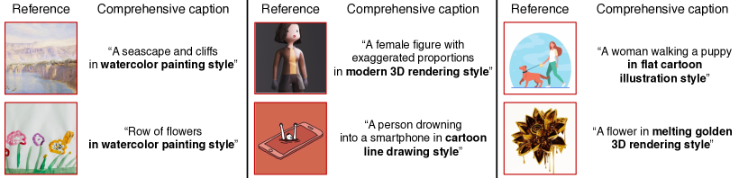
Figure 12: Examples of comprehensive caption for style images. We provide the examples of reference style images and comprehensive captions for style personalization experiment. To disentangle the subject and style in the image, we provide comprehensive description to the subject of the image. The texts marked in bold are used to generate image in custom style.

D.2 Evaluation Prompt

We construct two types of evaluation prompts; (1) subject customization, and (2) subject stylization. In evaluating subject customization, we provide the textual prompts that alter the attributes of the subject (e.g., “cube-shaped”) or its background (e.g., “on the beach”) following DreamBooth (Ruiz et al., 2023a). In evaluating subject stylization, we provide the textual prompts that stylizes the subject into different styles (e.g., “in watercolor painting style”, “in origami style”). For fine-grained evaluation, we construct different prompts for each object (e.g., “clock”, “robot toy”) and subject (e.g., “cat”, “dog”, “wolf plushie”). The examples of evaluation prompts for each category and type are in Table 2.

Table 2: Examples of evaluation prompts used to synthesize images for each object and live subject category. Subject customization are prompts to generate novel views of photo-realistic images and subject stylization aims to alter style of the subject. {}’s are filled with the class token of the subject.

Category\Type	Subject customization	Subject stylization
Object	“A photo of {} on the beach”	“A {} in sticker style”
	“A photo of {} with ribbons”	“A {} in wooden sculpture”
	“A photo of cube-shaped {}”	“A {} in flat cartoon illustration style”
	“A photo of golden {}”	“A {} in pixel art style”
	“A photo of {} made out of leathers”	“A {} in wireframe 3D style”
	“A photo of {} with a tree and autumn leaves in the background”	“A {} in hygge style”
	“A photo of {} on top of a white rug”	“A {} in geometric art style”
Subject	“A photo of {} wearing a spacesuit, planting a flag on the moon”	“A {} playing a violin in sticker style.”
	“A photo of {} as a firefighter, extinguishing a fire in a skyscraper”	“A {} carved as a knight in wooden sculpture”
	“A photo of {} in a wetsuit, surfing a giant wave in the ocea”	“A {} piloting a hot air balloon in travel agency logo style”
	“A photo of {} in Victorian attire, attending a tea party in an elegant garden”	“A {} constructed from abstract metal shapes in constructivism style”
	“A photo of {} in a snowsuit, skiing down a steep mountain”	“A {} on an epic quest in pixel art style”
	“A photo of {} as an explorer, navigating through an icy Arctic landscape”	“A {} designed as an intricate machine in blueprint style”
	“A photo of {} in an elegant masquerade mask at a Venetian ball”	“A {} illustrated in an educational infographic style”

D.3 Hyperparameter detail

Training is performed on a single gpu (e.g., A100) using a batch size of $1$. We perform up to $2000$ optimization steps. Note that our approach is robust to the length of training steps compared to the baseline (i.e., DreamBooth), which often requires early stopping to prevent overfitting. We fine-tune LoRA of rank 32 for subject personalization and rank 64 for style personalization. For sampling, we use DDIM (Song et al., 2020a) scheduler with 50 steps, and use CFG guidance scale of $7.5$ throughout experiments.

D.4 Evaluation metric

To measure the image similarity, we use DINOv2 (Oquab et al., 2023) score, which is given by the mean cosine similarity between the embeddings of reference images and synthesized images. To measure the image-text similarity, we use SigLIP (Zhai et al., 2023) score, which is defined as

$$S_{IT}(\mathbf{x},\mathbf{c})=\frac{1}{1+\exp\big{(}-f_{\textrm{img}}(\mathbf{x})^{\top}f_{\textrm{text}}(\mathbf{c})+b\big{)}}$$

where $f_{\textrm{img}}$ and $f_{\textrm{text}}$ are $\ell_{2}$ normalized embeddings from image and text encoders, and $b$ is a bias term that is optimized during pretraining. We opt to use SigLIP score instead of CLIP score (Radford et al., 2021), as the range of CLIP score depends on the prompt and images, while SigLIP score provides a general score that is bounded on $[0,1]$. For style personalization experiment, we measure image similarity using SigLIP image similarity, by computing the embeddings with SigLIP image encoder. While we desire high scores, these metrics are not perfect, e.g., the image similarity can get $1.0$ if the model overfits, otherwise, the image-text similarity can achieve high score if the model underfits. Thus, instead of reporting the scores from a single data point, we provide multiple data points of the same model while varying sampling parameters (e.g., guidance scale values of reward guidance sampling) and show the trends (e.g., by showing the Pareto frontier).

D.5 Computational Efficiency

Here, we provide some additional information about our method in terms of computational efficiency. Since our method leverages inference on pretrained model during training (e.g., Algorithm 1) and inference (when using reward guidance sampling) (e.g., Eq. (13)), there exists a few extra computational burden compared to original DreamBooth fine-tuning or CFG sampling. Specifically, we measured the optimization and inference time per iteration. Compared to DreamBooth, our method (DCO) approximately takes $\times 1.3$ longer time in fine-tuning. Compared to CFG sampling, reward guidance sampling requires $\times 2$ longer time in sampling. We believe that our work will motivate future studies on efficient fine-tuning to enhance scalability in practical scenarios.

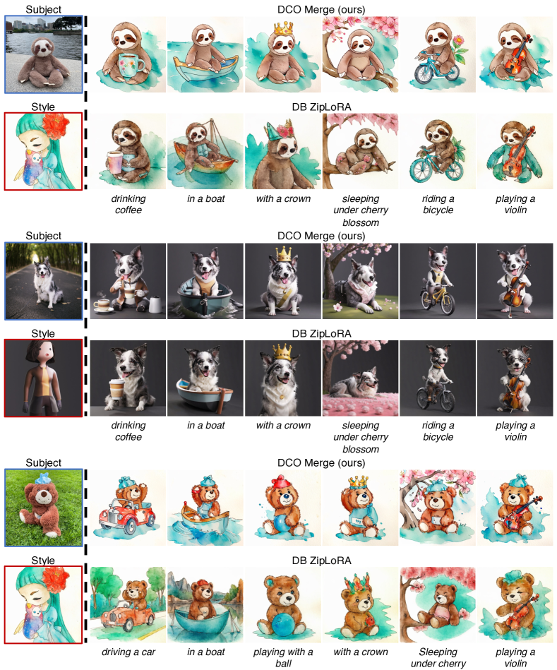
Figure 20: Text-compositional my subject in my style generation. (continued)

References

- Achiam et al. (2023) Achiam, J., Adler, S., Agarwal, S., Ahmad, L., Akkaya, I., Aleman, F. L., Almeida, D., Altenschmidt, J., Altman, S., Anadkat, S., et al. Gpt-4 technical report. arXiv preprint arXiv:2303.08774, 2023.
- Arar et al. (2024) Arar, M., Voynov, A., Hertz, A., Avrahami, O., Fruchter, S., Pritch, Y., Cohen-Or, D., and Shamir, A. Palp: Prompt aligned personalization of text-to-image models. arXiv preprint arXiv:2401.06105, 2024.
- Avrahami et al. (2023) Avrahami, O., Hertz, A., Vinker, Y., Arar, M., Fruchter, S., Fried, O., Cohen-Or, D., and Lischinski, D. The chosen one: Consistent characters in text-to-image diffusion models. arXiv preprint arXiv:2311.10093, 2023.
- Betker et al. (2023) Betker, J., Goh, G., Jing, L., Brooks, T., Wang, J., Li, L., Ouyang, L., Zhuang, J., Lee, J., Guo, Y., et al. Improving image generation with better captions. Computer Science. https://cdn. openai. com/papers/dall-e-3. pdf, 2:3, 2023.
- Black et al. (2023) Black, K., Janner, M., Du, Y., Kostrikov, I., and Levine, S. Training diffusion models with reinforcement learning. arXiv preprint arXiv:2305.13301, 2023.
- Chang et al. (2023) Chang, H., Zhang, H., Barber, J., Maschinot, A., Lezama, J., Jiang, L., Yang, M.-H., Murphy, K., Freeman, W. T., Rubinstein, M., et al. Muse: Text-to-image generation via masked generative transformers. arXiv preprint arXiv:2301.00704, 2023.
- Clark et al. (2023) Clark, K., Vicol, P., Swersky, K., and Fleet, D. J. Directly fine-tuning diffusion models on differentiable rewards. arXiv preprint arXiv:2309.17400, 2023.
- Dai et al. (2023) Dai, X., Hou, J., Ma, C.-Y., Tsai, S., Wang, J., Wang, R., Zhang, P., Vandenhende, S., Wang, X., Dubey, A., et al. Emu: Enhancing image generation models using photogenic needles in a haystack. arXiv preprint arXiv:2309.15807, 2023.
- Dong et al. (2023) Dong, H., Xiong, W., Goyal, D., Pan, R., Diao, S., Zhang, J., Shum, K., and Zhang, T. Raft: Reward ranked finetuning for generative foundation model alignment. arXiv preprint arXiv:2304.06767, 2023.
- Fan et al. (2023) Fan, Y., Watkins, O., Du, Y., Liu, H., Ryu, M., Boutilier, C., Abbeel, P., Ghavamzadeh, M., Lee, K., and Lee, K. Dpok: Reinforcement learning for fine-tuning text-to-image diffusion models. arXiv preprint arXiv:2305.16381, 2023.
- Gal et al. (2022) Gal, R., Alaluf, Y., Atzmon, Y., Patashnik, O., Bermano, A. H., Chechik, G., and Cohen-Or, D. An image is worth one word: Personalizing text-to-image generation using textual inversion. arXiv preprint arXiv:2208.01618, 2022.
- Gal et al. (2023) Gal, R., Arar, M., Atzmon, Y., Bermano, A. H., Chechik, G., and Cohen-Or, D. Designing an encoder for fast personalization of text-to-image models. arXiv preprint arXiv:2302.12228, 2023.
- Gu et al. (2023) Gu, Y., Wang, X., Wu, J. Z., Shi, Y., Chen, Y., Fan, Z., Xiao, W., Zhao, R., Chang, S., Wu, W., et al. Mix-of-show: Decentralized low-rank adaptation for multi-concept customization of diffusion models. arXiv preprint arXiv:2305.18292, 2023.
- Guttenberg (2023) Guttenberg, N. Diffusion with offset noise. link, 2023.
- Han et al. (2023) Han, L., Li, Y., Zhang, H., Milanfar, P., Metaxas, D., and Yang, F. Svdiff: Compact parameter space for diffusion fine-tuning. arXiv preprint arXiv:2303.11305, 2023.
- Hertz et al. (2023) Hertz, A., Voynov, A., Fruchter, S., and Cohen-Or, D. Style aligned image generation via shared attention. arXiv preprint arXiv:2312.02133, 2023.
- Ho & Salimans (2022) Ho, J. and Salimans, T. Classifier-free diffusion guidance. arXiv preprint arXiv:2207.12598, 2022.
- Ho et al. (2020) Ho, J., Jain, A., and Abbeel, P. Denoising diffusion probabilistic models. Advances in neural information processing systems, 33:6840–6851, 2020.
- Houlsby et al. (2019) Houlsby, N., Giurgiu, A., Jastrzebski, S., Morrone, B., De Laroussilhe, Q., Gesmundo, A., Attariyan, M., and Gelly, S. Parameter-efficient transfer learning for nlp. In International Conference on Machine Learning, pp. 2790–2799. PMLR, 2019.
- Hu et al. (2021) Hu, E. J., Shen, Y., Wallis, P., Allen-Zhu, Z., Li, Y., Wang, S., Wang, L., and Chen, W. Lora: Low-rank adaptation of large language models. arXiv preprint arXiv:2106.09685, 2021.
- Huang et al. (2023) Huang, Z., Wu, T., Jiang, Y., Chan, K. C., and Liu, Z. Reversion: Diffusion-based relation inversion from images. arXiv preprint arXiv:2303.13495, 2023.
- Hyvärinen & Dayan (2005) Hyvärinen, A. and Dayan, P. Estimation of non-normalized statistical models by score matching. Journal of Machine Learning Research, 6(4), 2005.
- Karras et al. (2022) Karras, T., Aittala, M., Aila, T., and Laine, S. Elucidating the design space of diffusion-based generative models. Advances in Neural Information Processing Systems, 35:26565–26577, 2022.
- Kim et al. (2022) Kim, D., Kim, Y., Kwon, S. J., Kang, W., and Moon, I.-C. Refining generative process with discriminator guidance in score-based diffusion models. arXiv preprint arXiv:2211.17091, 2022.
- Kingma et al. (2021) Kingma, D., Salimans, T., Poole, B., and Ho, J. Variational diffusion models. Advances in neural information processing systems, 34:21696–21707, 2021.
- Kingma & Ba (2014) Kingma, D. P. and Ba, J. Adam: A method for stochastic optimization. arXiv preprint arXiv:1412.6980, 2014.
- Kingma & Gao (2023) Kingma, D. P. and Gao, R. Understanding diffusion objectives as the elbo with simple data augmentation. In Thirty-seventh Conference on Neural Information Processing Systems, 2023.
- Kirstain et al. (2023) Kirstain, Y., Polyak, A., Singer, U., Matiana, S., Penna, J., and Levy, O. Pick-a-pic: An open dataset of user preferences for text-to-image generation. arXiv preprint arXiv:2305.01569, 2023.
- Kumari et al. (2023) Kumari, N., Zhang, B., Zhang, R., Shechtman, E., and Zhu, J.-Y. Multi-concept customization of text-to-image diffusion. In Proceedings of the IEEE/CVF Conference on Computer Vision and Pattern Recognition, pp. 1931–1941, 2023.
- Lee et al. (2023) Lee, K., Liu, H., Ryu, M., Watkins, O., Du, Y., Boutilier, C., Abbeel, P., Ghavamzadeh, M., and Gu, S. S. Aligning text-to-image models using human feedback. arXiv preprint arXiv:2302.12192, 2023.
- Liu et al. (2023) Liu, H., Li, C., Wu, Q., and Lee, Y. J. Visual instruction tuning. arXiv preprint arXiv:2304.08485, 2023.
- Liu et al. (2022) Liu, N., Li, S., Du, Y., Torralba, A., and Tenenbaum, J. B. Compositional visual generation with composable diffusion models. In European Conference on Computer Vision, pp. 423–439. Springer, 2022.
- Lu et al. (2023) Lu, C., Chen, H., Chen, J., Su, H., Li, C., and Zhu, J. Contrastive energy prediction for exact energy-guided diffusion sampling in offline reinforcement learning. arXiv preprint arXiv:2304.12824, 2023.
- Nichol et al. (2021) Nichol, A., Dhariwal, P., Ramesh, A., Shyam, P., Mishkin, P., McGrew, B., Sutskever, I., and Chen, M. Glide: Towards photorealistic image generation and editing with text-guided diffusion models. arXiv preprint arXiv:2112.10741, 2021.
- Oquab et al. (2023) Oquab, M., Darcet, T., Moutakanni, T., Vo, H., Szafraniec, M., Khalidov, V., Fernandez, P., Haziza, D., Massa, F., El-Nouby, A., et al. Dinov2: Learning robust visual features without supervision. arXiv preprint arXiv:2304.07193, 2023.
- Peters et al. (2010) Peters, J., Mulling, K., and Altun, Y. Relative entropy policy search. In Proceedings of the AAAI Conference on Artificial Intelligence, volume 24, pp. 1607–1612, 2010.
- Po et al. (2023) Po, R., Yang, G., Aberman, K., and Wetzstein, G. Orthogonal adaptation for modular customization of diffusion models. arXiv preprint arXiv:2312.02432, 2023.
- Podell et al. (2023) Podell, D., English, Z., Lacey, K., Blattmann, A., Dockhorn, T., Müller, J., Penna, J., and Rombach, R. Sdxl: Improving latent diffusion models for high-resolution image synthesis. arXiv preprint arXiv:2307.01952, 2023.
- Prabhudesai et al. (2023) Prabhudesai, M., Goyal, A., Pathak, D., and Fragkiadaki, K. Aligning text-to-image diffusion models with reward backpropagation. arXiv preprint arXiv:2310.03739, 2023.
- Radford et al. (2021) Radford, A., Kim, J. W., Hallacy, C., Ramesh, A., Goh, G., Agarwal, S., Sastry, G., Askell, A., Mishkin, P., Clark, J., et al. Learning transferable visual models from natural language supervision. In International conference on machine learning, pp. 8748–8763. PMLR, 2021.
- Rafailov et al. (2023) Rafailov, R., Sharma, A., Mitchell, E., Ermon, S., Manning, C. D., and Finn, C. Direct preference optimization: Your language model is secretly a reward model. arXiv preprint arXiv:2305.18290, 2023.
- Raffel et al. (2020) Raffel, C., Shazeer, N., Roberts, A., Lee, K., Narang, S., Matena, M., Zhou, Y., Li, W., and Liu, P. J. Exploring the limits of transfer learning with a unified text-to-text transformer. The Journal of Machine Learning Research, 21(1):5485–5551, 2020.
- Ramesh et al. (2021) Ramesh, A., Pavlov, M., Goh, G., Gray, S., Voss, C., Radford, A., Chen, M., and Sutskever, I. Zero-shot text-to-image generation. In International Conference on Machine Learning, pp. 8821–8831. PMLR, 2021.
- Ramesh et al. (2022) Ramesh, A., Dhariwal, P., Nichol, A., Chu, C., and Chen, M. Hierarchical text-conditional image generation with clip latents. arXiv preprint arXiv:2204.06125, 1(2):3, 2022.
- Rombach et al. (2022) Rombach, R., Blattmann, A., Lorenz, D., Esser, P., and Ommer, B. High-resolution image synthesis with latent diffusion models. In Proceedings of the IEEE/CVF conference on computer vision and pattern recognition, pp. 10684–10695, 2022.
- Ruiz et al. (2023a) Ruiz, N., Li, Y., Jampani, V., Pritch, Y., Rubinstein, M., and Aberman, K. Dreambooth: Fine tuning text-to-image diffusion models for subject-driven generation. In Proceedings of the IEEE/CVF Conference on Computer Vision and Pattern Recognition, pp. 22500–22510, 2023a.
- Ruiz et al. (2023b) Ruiz, N., Li, Y., Jampani, V., Wei, W., Hou, T., Pritch, Y., Wadhwa, N., Rubinstein, M., and Aberman, K. Hyperdreambooth: Hypernetworks for fast personalization of text-to-image models. arXiv preprint arXiv:2307.06949, 2023b.
- Ryu (2023) Ryu, S. Low-rank adaptation for fast text-to-image diffusion fine-tuning, 2023.
- Saharia et al. (2022) Saharia, C., Chan, W., Saxena, S., Li, L., Whang, J., Denton, E. L., Ghasemipour, K., Gontijo Lopes, R., Karagol Ayan, B., Salimans, T., et al. Photorealistic text-to-image diffusion models with deep language understanding. Advances in Neural Information Processing Systems, 35:36479–36494, 2022.
- Schuhmann & Beaumont (2022) Schuhmann, C. and Beaumont, R. Laion-aesthetics, 2022.
- Shah et al. (2023) Shah, V., Ruiz, N., Cole, F., Lu, E., Lazebnik, S., Li, Y., and Jampani, V. Ziplora: Any subject in any style by effectively merging loras. arXiv preprint arXiv:2311.13600, 2023.
- Sohn et al. (2023) Sohn, K., Ruiz, N., Lee, K., Chin, D. C., Blok, I., Chang, H., Barber, J., Jiang, L., Entis, G., Li, Y., et al. Styledrop: Text-to-image generation in any style. arXiv preprint arXiv:2306.00983, 2023.
- Song et al. (2020a) Song, J., Meng, C., and Ermon, S. Denoising diffusion implicit models. arXiv preprint arXiv:2010.02502, 2020a.
- Song et al. (2020b) Song, Y., Sohl-Dickstein, J., Kingma, D. P., Kumar, A., Ermon, S., and Poole, B. Score-based generative modeling through stochastic differential equations. arXiv preprint arXiv:2011.13456, 2020b.
- Tang et al. (2023) Tang, L., Ruiz, N., Chu, Q., Li, Y., Holynski, A., Jacobs, D. E., Hariharan, B., Pritch, Y., Wadhwa, N., Aberman, K., et al. Realfill: Reference-driven generation for authentic image completion. arXiv preprint arXiv:2309.16668, 2023.
- Tewel et al. (2023) Tewel, Y., Gal, R., Chechik, G., and Atzmon, Y. Key-locked rank one editing for text-to-image personalization. In ACM SIGGRAPH 2023 Conference Proceedings, pp. 1–11, 2023.
- Tewel et al. (2024) Tewel, Y., Kaduri, O., Gal, R., Kasten, Y., Wolf, L., Chechik, G., and Atzmon, Y. Training-free consistent text-to-image generation, 2024.
- Voynov et al. (2023) Voynov, A., Chu, Q., Cohen-Or, D., and Aberman, K. : Extended textual conditioning in text-to-image generation. arXiv preprint arXiv:2303.09522, 2023.
- Wallace et al. (2023) Wallace, B., Dang, M., Rafailov, R., Zhou, L., Lou, A., Purushwalkam, S., Ermon, S., Xiong, C., Joty, S., and Naik, N. Diffusion model alignment using direct preference optimization. arXiv preprint arXiv:2311.12908, 2023.
- Wei et al. (2023) Wei, Y., Zhang, Y., Ji, Z., Bai, J., Zhang, L., and Zuo, W. Elite: Encoding visual concepts into textual embeddings for customized text-to-image generation. arXiv preprint arXiv:2302.13848, 2023.
- Wu et al. (2019) Wu, Y., Tucker, G., and Nachum, O. Behavior regularized offline reinforcement learning. arXiv preprint arXiv:1911.11361, 2019.
- Xu et al. (2023) Xu, J., Liu, X., Wu, Y., Tong, Y., Li, Q., Ding, M., Tang, J., and Dong, Y. Imagereward: Learning and evaluating human preferences for text-to-image generation. arXiv preprint arXiv:2304.05977, 2023.
- Yu et al. (2022) Yu, J., Xu, Y., Koh, J. Y., Luong, T., Baid, G., Wang, Z., Vasudevan, V., Ku, A., Yang, Y., Ayan, B. K., et al. Scaling autoregressive models for content-rich text-to-image generation. arXiv preprint arXiv:2206.10789, 2(3):5, 2022.
- Zhai et al. (2023) Zhai, X., Mustafa, B., Kolesnikov, A., and Beyer, L. Sigmoid loss for language image pre-training. arXiv preprint arXiv:2303.15343, 2023.