Global stability and optimal control in a single-strain dengue model with fractional-order transmission and recovery process

Abstract

In this manuscript, we developed a novel single strain dengue model with fractional order transmission and recovery from a stochastic process. Fractional derivative appeared in the disease transmission and recovery processes is known as tempered fractional ($TF$) derivative. We showed that if a function satisfying certain conditions, then $TF$ derivative of that function is proportional to the function itself. By utilizing this result, we investigated the local and global stability of various equilibrium solutions (disease-free and endemic) related to the novel fractional-order dengue model in terms of the basic reproduction number $R_{0}$. Additionally, we developed an optimal control problem for the extended fractional-order dengue system with control to study the effect of three different interventions: reduction of mosquito recruitment rate, adult vector control, and individual protection. Furthermore, we derived a sufficient condition for the existence of a solution to the optimal control problem. Finally, numerical experiments suggest that policymakers may focus on fractional-order parameters that represent the mechanisms of disease transmission and recovery in addition to the two vector controls to reduce dengue spreading in a location.

1 Introduction

The viral infection dengue transmitted to human due to the bite of female Aedes aegypti mosquito carrying any one of the four virus serotypes namely DENV-1, DENV-2, DENV-3, and DENV-4 WHO-DEN09 ; gubler1995dengue . An infected vector stays infected and never fully recovers from the infection because mosquitoes have a short lifespan sardar2015mathematical . The past few decades have seen an increase in dengue fever cases worldwide as a result of rising temperatures ong2021adult . According to some estimates, there are 390 million dengue infections annually in the world, of which 96 million result in clinical symptoms bhatt2013global . The dengue virus is an acute febrile viral illness that frequently causes headaches, rash, pain in the muscles and bones, and flu-like symptoms htun2021clinical . However, dengue hemorrhagic fever (DHF) or dengue shock syndrome (DSS) is a potentially fatal form of the illness that can cause bleeding, vomiting, and an abrupt drop in blood pressure WHO-DEN09 ; htun2021clinical . Cases of the severe form of dengue hemorrhagic fever (DHF) rose sharply each year throughout the world WHO-DEN09 . The most affected areas by dengue fever are Latin America, the Eastern Mediterranean, Africa, the Western Pacific region, South-East Asia, and the subtropical regions of the world WHO-DEN09 ; gubler2002epidemic ; pinheiro1997global . Controlling the vector population and adopting personal protective measures are two potential intervention strategies for dengue fever, as there is currently no known treatment or vaccine WHO-DEN09 . Therefore, in order to offer a more insightful interpretation of the mechanism of dengue transmission and effect of different interventions, a suitable mathematical model is necessary andraud2012dynamic ; aguiar2022mathematical .

Over the past ten years, various statistical and mathematical models on dengue fever have been developed, offering valuable insights into the spread of the disease and its management andraud2012dynamic ; aguiar2022mathematical ; pinho2010modelling ; gubler2002epidemic . However, the authors of the majority of these models assume that the transmission and recovery processes follow an exponential distribution, which results in a coupled ordinary differential equation system andraud2012dynamic ; aguiar2022mathematical ; pinho2010modelling ; gubler2002epidemic . The solution generated from such a system in general follows a Markovian process agarwal2013existence ; podlubny1999fractional ; du2013measuring ; dokoumetzidis2009fractional ; dokoumetzidis2010fractional ; sardar2015mathematical . However, disease transmission typically occurs through a non-markovian mechanism saeedian2017memory ; starnini2017equivalence ; angstmann2016fractional ; sardar2015mathematical ; sardar2017mathematical . Thus, a mathematical model of dengue fever developed with the assumption of non-Markovian transmission may provide some useful information on the disease’s spread and control angstmann2016fractional ; sardar2017mathematical ; angstmann2017fractional .

A few mathematical models of infectious diseases assuming non-Markovian transmission can be found in the literature sardar2015mathematical ; angstmann2016fractional ; angstmann2017fractional ; sardar2017mathematical ; angstmann2021general ; wu2023global . However, we could only identify two publications that develop mathematical models with non-Markovian transmission about dengue fever or vector-borne diseases sardar2015mathematical ; sardar2017mathematical . In sardar2015mathematical , authors first convert a simple deterministic vector-borne disease model to a system of integral equations. Then they introduced some time-dependent integral kernels in two forces of infection. Furthermore, the authors showed that when time-dependent kernels follow some power-law form, the deterministic dengue system converts to a fractional-order system. Moreover, by studying the local stability properties of different equilibrium solutions of the fractional order system, the authors proved that conventional epidemiological results do not hold for such systems, as reducing the basic reproduction number ($R_{0}$) below one may not be sufficient for the eradication of dengue fever sardar2015mathematical . In sardar2017mathematical , authors follow the approach introduced by Angstmann et al. angstmann2016fractional ; angstmann2017fractional to develop a fractional-order dengue compartmental system directly from a stochastic process. In their model sardar2017mathematical , fractional derivative appeared in the force of infection due to the assumption that the disease transmission follows some power-law (non-Markovian) distribution. Furthermore, the authors investigate the local stability of different equilibrium solutions and calibrate the fractional order dengue system to some real-life data sardar2017mathematical .

Some recent epidemiological findings indicate that both the transmission and recovery processes may exhibit a non-Markovian mechanism starnini2017equivalence ; lin2020non ; sherborne2018mean . However, in the context of dengue fever or any other vector-borne disease, a mathematical model with a non-Markovian transmission and recovery mechanism seems rare. Furthermore, we found only one work that mathematically analyzed the global stability of different equilibrium points of a $SIS$ epidemic model with fractional order transmission wu2023global . However, in wu2023global , authors considered only linear fractional-order infection terms, which is different from other models developed in this direction angstmann2016fractional ; angstmann2017fractional ; angstmann2021general . Furthermore, as far as we are aware, there is not much research done on optimal control problems for these types of mathematical models, where transmission and recovery processes follow some kind of fractional-order dynamics.

The three main objectives of this work are provided below:

1. Development of a new mathematical model for dengue fever with fractional-order transmission and recovery processes.

2. Provide mathematical proof of the local and global stability of different equilibrium solutions to this new fractional-order dengue model.

3. We attempt to formulate and analyze an optimal control problem associated with this new fractional-order dengue model in order to investigate the effects of various dengue interventions.

The rest of the paper is arranged as follows: In Section 2, we made available various definitions and proofs of some results that will be used throughout the manuscript. A new single-strain dengue model with fractional-order transmission and recovery is developed in Section 3. Some mathematical properties like positive invariance and boundedness of solution of the new fractional-order dengue model are studied in Section 4. In Section 5, we investigate the local and global stability of different equilibrium points of the newly developed model with fractional-order transmission and recovery processes. The development of an optimal control problem related to the fractional-order dengue model is provided in Section 6. A numerical investigation of this new fractional-order dengue model along with the optimal control problem is provided in Section 7. Finally, the paper ends with a brief discussion and summary of the main results in Section 8.

2 Preliminaries

In this section, we incorporate several definitions, lemmas, and theorems that are used in different sections of this manuscript. The Riemann-Liouville (R-L) and the Caputo fractional derivatives of a smooth real function $f(t)$ of order $\alpha$ (see (podlubny1999fractional, )), where, $0<\alpha<1$, are defined as follows:

      Definition 2.1.

(R-L fractional integral) The Riemann-Liouville fractional Integral is defined as:

$$\ _{RL}I_{t}^{\alpha}\left[f(t)\right] =\frac{1}{\Gamma(\alpha)}\int_{0}^{t}(t-u)^{\alpha-1}f(u)du$$ (2.1)

      Definition 2.2.

(R-L fractional derivative) The Riemann-Liouville fractional Derivative is defined as:

$$\ {}_{RL}D_{t}^{\alpha}\left[f(t)\right] =\displaystyle\frac{1}{\Gamma(1-\alpha)}\frac{d}{dt}\int_{0}^{t}(t-u)^{-\alpha}f(u)du.$$ (2.2)

      Definition 2.3.

(Caputo fractional derivative) The Caputo fractional derivative is defined as:

$$\ {}_{C}D_{t}^{\alpha}\left[f(t)\right] =\displaystyle\frac{1}{\Gamma(1-\alpha)}\int_{0}^{t}(t-u)^{-\alpha}f^{\prime}(u)du.$$ (2.3)

Relation between the R-L and the Caputo fractional derivatives and their Laplace transformations (see podlubny1999fractional ) are provided below:

$$\ {}_{RL}D_{t}^{\alpha}\left[f(t)\right] =\ {}_{C}D_{t}^{\alpha}\left[f(t)\right]+\frac{f(0)t^{-\alpha}}{\Gamma(1-\alpha)},$$ (2.4)

and

$$\displaystyle L\left[\ {}_{RL}D_{t}^{\alpha}\left(f(t)\right);s\right] =\displaystyle s^{\alpha}L[f(t)].$$ (2.5)

      Definition 2.4.

The lower incomplete gamma function $\gamma(x,\alpha)$, with $\alpha>0$, and $x\geq 0$ is defined as follows:

$$\ \gamma(x,\alpha):=\int_{0}^{x}u^{\alpha-1}e^{-u}du$$ (2.6)

Remark 2.1.

The following integral relation holds:

$$\int_{t_{1}}^{t_{2}}(t-\tau)^{\alpha-1}e^{-l(t-\tau)}d\tau =\displaystyle\frac{1}{l^{\alpha}}\Bigg{[}\gamma\Big{(}l(t-t_{1}),\alpha\Big{)}-\gamma\Big{(}l(t-t_{2}),\alpha\Big{)}\Bigg{]},$$ (2.7)

where, $t_{1},t_{2}>0$.

Theorem 2.1.

Let $F\in\mathbb{C}[0,T]$, $F(t)\geq 0\;\mbox{for all}\;t\geq 0$ and $\beta>0$, then we have, $e^{-\beta t}\ _{RL}D_{t}^{\alpha}\left[e^{\beta t}F(t)\right]\approx\beta^{\alpha}F(t)$.

Proof.

Note that,

$$e^{{-\beta}t}\ _{RL}I_{t}^{\alpha}\left[e^{\beta t}F(t)\right]=\frac{1}{\Gamma(\alpha)}\int_{0}^{t}(t-u)^{\alpha-1}e^{-\beta\left(t-u\right)}F(u)du,$$

Since, $F\in\mathbb{C}[0,t]$, and $g(t)=t^{\alpha-1}e^{-\beta t}$ is an integrable function which does not change sign in $[0,t]$, therefore, applying Mean Value Theorem of definite integrals we have

$$e^{-\beta t}\ _{RL}I_{t}^{\alpha}\left[e^{\beta t}F(t)\right] =\frac{1}{\Gamma(\alpha)}F(\xi)\int_{0}^{t}(t-u)^{\alpha-1}e^{-\beta\left(t-u\right)}du,\leavevmode\nobreak\ \leavevmode\nobreak\ \text{where}\leavevmode\nobreak\ {}\xi\in(0,t)$$ (2.8)

$$=\frac{1}{\Gamma(\alpha)}F(\xi)\frac{\gamma(\beta t,\alpha)}{\beta^{\alpha}},\leavevmode\nobreak\ \hskip 28.45274pt\text{using Remark}\leavevmode\nobreak\ (\ref{Definition-4}),$$

$$\implies\ _{RL}I_{t}^{\alpha}\left[e^{\beta t}F(t)\right] =\frac{e^{\beta t}}{\Gamma(\alpha)}F(\xi)\frac{\gamma(\beta t,\alpha)}{\beta^{\alpha}},$$

$$\implies e^{\beta t}F(t) =\ _{RL}D_{t}^{\alpha}\left[\frac{e^{\beta t}}{\Gamma(\alpha)}F(\xi)\frac{\gamma(\beta t,\alpha)}{\beta^{\alpha}}\right],$$

$$\implies\beta^{\alpha}F(t) =\frac{e^{-\beta t}}{\Gamma(\alpha)}\ _{RL}D_{t}^{\alpha}\left[e^{\beta t}F(\xi)\gamma(\beta t,\alpha)\right],$$

$$=\frac{e^{-\beta t}}{\Gamma(\alpha)}\frac{1}{\Gamma(1-\alpha)}\frac{d}{dt}\int_{0}^{t}(t-u)^{-\alpha}e^{\beta u}F(u)\gamma(\beta u,\alpha)du.$$

Again, $\gamma(\beta t,\alpha)$ is a continuous function and as $F(t)\geq 0\leavevmode\nobreak\ \leavevmode\nobreak\ \mbox{for all}\;t\geq 0$, therefore, $(t-u)^{-\alpha}e^{\beta u}F(u)$, where, $0<u<t$, is integrable and do not changes sign in $[0,t]$. Thus, applying Mean Value Theorem of definite integrals we have,

$$\leavevmode\nobreak\ \beta^{\alpha}F(t) =\frac{e^{-\beta t}}{\Gamma(\alpha)}\frac{1}{\Gamma(1-\alpha)}\frac{d}{dt}\left[\gamma(\beta\xi_{1},\alpha)\int_{0}^{t}(t-u)^{-\alpha}e^{\beta u}F(u)du\right],\leavevmode\nobreak\ \leavevmode\nobreak\ \text{where}\leavevmode\nobreak\ \leavevmode\nobreak\ {}\xi_{1}\in(0,t),$$ (2.9)

$$=\frac{\gamma(\beta\xi_{1},\alpha)}{\Gamma(\alpha)}e^{-\beta t}\ _{RL}D_{t}^{\alpha}\left[e^{\beta t}F(t)\right]+\frac{e^{-\beta\xi_{1}}\left(\beta\xi_{1}\right)^{\alpha-1}\gamma(\beta t,1-\alpha)}{\beta^{\alpha}\Gamma(\alpha)\Gamma(1-\alpha)}F(\xi_{2})\leavevmode\nobreak\ \hskip 2.84544pt\text{where,}\leavevmode\nobreak\ {}\xi_{1},\xi_{2}\in(0,t).$$

Now, $\frac{\gamma(\beta t,1-\alpha)}{\Gamma(1-\alpha)}\to 1$ as $t\to\infty$ and $e^{-\beta\xi_{1}}\left(\beta\xi_{1}\right)^{\alpha-1}\to 0$ as $t\to\infty$. Hence (2.9) can be written as

$$e^{-\beta t}\ _{RL}D_{t}^{\alpha}\left[e^{\beta t}F(t)\right] \approx\beta^{\alpha}F(t).$$

∎

3 Model formulation

To develop a vector-borne disease model with fractional-order transmission and recovery process, the following assumptions are made:

1. Total human population $N_{H}$ is constant.

2. Average biting rate is $\frac{b}{N_{H}}$.

3. $\displaystyle\rho_{V}(t-\tau)$ is the intrinsic infection age in an infected vector. This function depend on both current time $t$, and time since infection $t-\tau$.

4. $\displaystyle\rho_{H}(t-\tau)$ is the intrinsic infection age in an infected human. This function depend on both current time $t$, and time since infection $t-\tau$.

5. Transmission probability from vector to human is $\beta_{V}^{H}$.

6. Transmission probability from human to vector is $\beta_{H}^{V}$.

7. Human population is subdivided into three mutually exclusive classes namely susceptible human ($S_{H}$), infected human ($I_{H}$), and recovered human ($R_{H}$), respectively.

8. Vector population is subdivided into two mutually exclusive classes namely susceptible vector ($S_{V}$), and infected vector ($I_{V}$), respectively.

9. Considering the short life span of the vector, we assumed no recovery for the infected vector population.

Now, the average number of newly infected humans generated within the time domain $[t,t+\Delta t]$ by a single vector infected at some earlier time $\tau<t$ is

$$\displaystyle\frac{b}{N_{H}}\beta_{V}^{H}\rho_{V}(t-\tau)S_{H}(t)\Delta t+o(\Delta t)$$ (3.1)

Following (sardar2017mathematical, ), we assume that the infection first occurred at time $t=0$. Furthermore, let $\Phi_{I_{V}}(t,\tau)$ be the survival probability of an infected vector at time $t$, provided it enters this compartment at time $\tau<t$. Therefore, the average number of newly infected humans at time $t$ is:

$$\displaystyle Q(I_{H},t) =\frac{b}{N_{H}}\beta_{V}^{H}S_{H}(t)\int_{0}^{t}\rho_{V}(t-\tau)\Phi_{I_{V}}(t,\tau)Q(I_{V},\tau)d\tau,$$ (3.2)

where, $Q(I_{V},t)$ is the average number of infected vector at time $t$.

An infected vector can move from its respective compartment only by natural death. We assume that the death process of vectors follows an exponential distribution. Therefore,

$$\displaystyle\Phi_{I_{V}}(t,\tau) =\displaystyle e^{-\int_{\tau}^{t}\mu_{v}ds}=\displaystyle e^{-\mu_{v}(t-\tau)},$$ (3.3)

where, $\mu_{v}$ is the natural death rate of the vectors.

The number of infected individuals at time $t$ is provided below:

$$\displaystyle I_{H}(t) =\displaystyle\int_{0}^{t}\Phi_{I_{H}}(t,\tau)Q(I_{H},\tau)d\tau,$$ (3.4)

where, $\Phi_{I_{H}}(t,\tau)$ is the survival probability of an infected individual who entered this compartment at time $\tau$, and will remain in this state up to time $t$ $(\tau<t)$. Furthermore, $Q(I_{H},t)$ is provided in equation (3.2).

From the hypothesis, there are two possible ways that an individual can move from the infected human compartment, either become recover from the disease or by natural death. We assume that these two processes are independent. Thus survival probability of an individual in the infected human compartment is provided below:

$$\displaystyle\Phi_{I_{H}}(t,\tau) =\displaystyle\phi_{h}^{R}(t-\tau)\theta_{h}^{D}(t,\tau),$$ (3.5)

where $\phi_{h}^{R}(t-\tau)$, and $\theta_{h}^{D}(t,\tau)$ are the probabilities that an individual has not recovered and died at time $t$, respectively, while they entered in this compartment ($I_{H}$) at time $\tau<t$. Furthermore, we assume the death process of humans follows the exponential distribution provided below:

$$\displaystyle\theta_{h}^{D}(t,\tau) =\displaystyle e^{-\int_{\tau}^{t}\mu_{H}ds}=\displaystyle e^{-\mu_{H}(t-\tau)},$$ (3.6)

where $\mu_{H}$ is the natural death rate of the human populations.

Therefore, using (3.5), we have from (3.4):

$$\displaystyle\frac{dI_{H}}{dt} =\displaystyle Q(I_{H},t)-\int_{0}^{t}\Psi(t-\tau)\theta_{h}^{D}(t,\tau)Q(I_{H},\tau)d\tau-\mu_{H}I_{H},$$ (3.7)

where $\displaystyle\Psi(t)=\displaystyle-\frac{d\phi_{h}^{R}(t)}{dt}$. Hence from  (3.2) we have:

$$\displaystyle\frac{dI_{H}}{dt} =\displaystyle\frac{b}{N_{H}}\beta_{V}^{H}S_{H}(t)\int_{0}^{t}\rho_{V}(t-\tau)\theta_{i_{v}}^{D}(t,\tau)Q(I_{V},\tau)d\tau$$ (3.8)

$$-\int_{0}^{t}\Psi(t-\tau)\theta_{h}^{D}(t,\tau)Q(I_{H},\tau)d\tau-\mu_{H}I_{H},$$

where $\theta_{i_{v}}^{D}(t,\tau)=e^{-\mu_{v}(t-\tau)}$.

Similarly, the average number of newly infected vector at time $t$ is:

$$\displaystyle Q(I_{V},t) =\frac{b}{N_{H}}\beta_{H}^{V}S_{V}(t)\int_{0}^{t}\rho_{H}(t-\tau)\Phi_{I_{H}}(t,\tau)Q(I_{H},\tau)d\tau,$$ (3.9)

where $Q(I_{H},t)$ is defined in equation (3.2). Using equation (3.5), we have:

$$\displaystyle Q(I_{V},t) =\frac{b}{N_{H}}\beta_{H}^{V}S_{V}(t)\int_{0}^{t}\rho_{H}(t-\tau)\phi_{h}^{R}(t-\tau)\theta_{h}^{D}(t,\tau)Q(I_{H},\tau)d\tau.$$ (3.10)

Therefore, the number of infected vectors at time $t$ is provided below:

$$\displaystyle I_{V}(t) =\displaystyle\int_{0}^{t}\Phi_{I_{V}}(t,\tau)Q(I_{V},\tau)d\tau.$$ (3.11)

Taking derivative in equation (3.11), and using the relation in (3.3) we have:

$$\displaystyle\frac{dI_{V}}{dt} =\displaystyle Q(I_{V},t)-\mu_{V}I_{V}.$$ (3.12)

Using relation (3.10), we have:

$$\displaystyle\frac{dI_{V}}{dt} =\displaystyle\frac{b}{N_{H}}\beta_{H}^{V}S_{V}(t)\int_{0}^{t}\rho_{H}(t-\tau)\phi_{h}^{R}(t-\tau)\theta_{h}^{D}(t,\tau)Q(I_{H},\tau)-\mu_{V}I_{V}.$$ (3.13)

Now $\theta_{h}^{D}(t,\tau)$, and $\theta_{i_{v}}^{D}(t,\tau)$ both satisfies semi-group property i.e.

$$\displaystyle\theta_{h}^{D}(t,\tau) =\displaystyle\theta_{h}^{D}(t,u)\theta_{h}^{D}(u,\tau),$$ (3.14)

$$\displaystyle\theta_{i_{v}}^{D}(t,\tau) =\displaystyle\theta_{i_{v}}^{D}(t,u)\theta_{i_{v}}^{D}(u,\tau),\hskip 11.38092pt\text{where}\hskip 11.38092pt\tau<u<t.$$

Using semi-group property the systems (3.8) and (3.13) become:

$$\displaystyle\frac{dI_{H}}{dt} =\displaystyle\frac{b}{N_{H}}\beta_{V}^{H}S_{H}(t)\theta_{i_{v}}^{D}(t,0)\int_{0}^{t}\rho_{V}(t-\tau)\frac{Q(I_{V},\tau)}{\theta_{i_{v}}^{D}(\tau,0)}d\tau$$ (3.15)

$$-\theta_{h}^{D}(t,0)\int_{0}^{t}\Psi(t-\tau)\frac{Q(I_{H},\tau)}{\theta_{h}^{D}(\tau,0)}d\tau-\mu_{H}I_{H}.$$

and

$$\displaystyle\frac{dI_{V}}{dt} =\displaystyle\frac{b}{N_{H}}\beta_{H}^{V}S_{V}(t)\theta_{h}^{D}(t,0)\int_{0}^{t}\rho_{H}(t-\tau)\phi_{h}^{R}(t-\tau)\frac{Q(I_{H},\tau)}{\theta_{h}^{D}(\tau,0)}d\tau-\mu_{V}I_{V}.$$ (3.16)

Now again using semi-group property (3.14), we have from (3.11):

$$\displaystyle\frac{I_{V}(t)}{\theta_{i_{v}}^{D}(t,0)} =\displaystyle\int_{0}^{t}\frac{Q(I_{V},\tau)}{\theta_{i_{v}}^{D}(\tau,0)}d\tau.$$ (3.17)

Taking Laplace transform w.r.t. $t$ in the both side of (3.17), we have:

$$\displaystyle L\left[\frac{I_{V}(t)}{\theta_{i_{v}}^{D}(t,0)}\right] =\displaystyle\frac{1}{s}L\left[\frac{Q(I_{V},t)}{\theta_{i_{v}}^{D}(t,0)}\right].$$ (3.18)

Therefore, from the first integrand in the right-hand side of the equation (3.15), we have:

$$\displaystyle L\left[\int_{0}^{t}\rho_{V}(t-\tau)\frac{Q(I_{V},\tau)}{\theta_{i_{v}}^{D}(\tau,0)}\right] =\displaystyle L\left[\kappa_{V}(t)\right]L\left[\frac{I_{V}(t)}{\theta_{i_{v}}^{D}(t,0)}\right],$$ (3.19)

$$=\int_{0}^{t}\kappa_{V}(t-\tau)\frac{I_{V}(\tau)}{\theta_{i_{v}}^{D}(\tau,0)}d\tau,$$

where

$$\displaystyle\kappa_{V}(t) =\displaystyle L^{-1}\left\{sL\left[\rho_{V}(t)\right]\right\}.$$ (3.20)

Again from (3.4), we have:

$$\displaystyle L\left[\frac{I_{H}(t)}{\theta_{h}^{D}(t,0)}\right] =\displaystyle L\left[\phi_{h}^{R}(t)\right]L\left[\frac{Q(I_{H},t)}{\theta_{h}^{D}(t,0)}\right].$$ (3.21)

Therefore, from the second integrand in the right-hand side of the equation (3.15), we have:

$$\displaystyle L\left[\int_{0}^{t}\Psi(t-\tau)\frac{Q(I_{H},\tau)}{\theta_{h}^{D}(\tau,0)}\right] =\displaystyle L\left[\kappa_{R}(t)\right]L\left[\frac{I_{H}(t)}{\theta_{h}^{D}(t,0)}\right],$$ (3.22)

$$=\int_{0}^{t}\kappa_{R}(t-\tau)\frac{I_{H}(\tau)}{\theta_{h}^{D}(\tau,0)}d\tau,$$

where

$$\displaystyle\kappa_{R}(t) =\displaystyle L^{-1}\left\{\frac{L\left[\Psi(t)\right]}{L\left[\phi_{h}^{R}(t)\right]}\right\}.$$ (3.23)

Therefore, using (3.19), and (3.22), we have the general integro-differential equation of the infected human compartment:

$$\displaystyle\frac{dI_{H}}{dt} =\displaystyle\frac{b}{N_{H}}\beta_{V}^{H}S_{H}(t)e^{-\mu_{V}t}\int_{0}^{t}\kappa_{V}(t-\tau)I_{V}(\tau)e^{\mu_{V}\tau}d\tau-e^{-\mu_{H}t}\int_{0}^{t}\kappa_{R}(t-\tau)I_{H}(\tau)e^{\mu_{H}\tau}d\tau$$ (3.24)

$$-\mu_{H}I_{H}.$$

Proceeding similarly, we have the general integro-differential equation of the infected vector compartment provided below:

$$\displaystyle\frac{dI_{V}}{dt} =\displaystyle\frac{b}{N_{H}}\beta_{H}^{V}S_{V}(t)e^{-\mu_{H}t}\int_{0}^{t}\kappa_{H}(t-\tau)I_{H}(\tau)e^{\mu_{H}\tau}d\tau-\mu_{V}I_{V},$$ (3.25)

where

$$\displaystyle\kappa_{H}(t) =\displaystyle L^{-1}\left\{\frac{L\left[\rho_{H}(t)\phi_{h}^{R}(t)\right]}{L\left[\phi_{h}^{R}(t)\right]}\right\},$$ (3.26)

Therefore, a general integro-differential equation representing the interaction between humans and vectors is provided below:

$$\displaystyle\frac{dS_{H}}{dt} =\mu_{H}N_{H}-\frac{b}{N_{H}}\beta_{V}^{H}S_{H}(t)e^{-\mu_{V}t}\int_{0}^{t}\kappa_{V}(t-\tau)I_{V}(\tau)e^{\mu_{V}\tau}d\tau-\mu_{H}S_{H},$$ (3.27)

$$\frac{dI_{H}}{dt} =\displaystyle\frac{b}{N_{H}}\beta_{V}^{H}S_{H}(t)e^{-\mu_{V}t}\int_{0}^{t}\kappa_{V}(t-\tau)I_{V}(\tau)e^{\mu_{V}\tau}d\tau-e^{-\mu_{H}t}\int_{0}^{t}\kappa_{R}(t-\tau)I_{H}(\tau)e^{\mu_{H}\tau}d\tau$$

$$-\mu_{H}I_{H},$$

$$\frac{dR_{H}}{dt} =\displaystyle e^{-\mu_{H}t}\int_{0}^{t}\kappa_{R}(t-\tau)I_{H}(\tau)e^{\mu_{H}\tau}d\tau-\mu_{H}R_{H},$$

$$\frac{dS_{V}}{dt} =\displaystyle\Pi_{V}-\frac{b}{N_{H}}\beta_{H}^{V}S_{V}(t)e^{-\mu_{H}t}\int_{0}^{t}\kappa_{H}(t-\tau)I_{H}(\tau)e^{\mu_{H}\tau}d\tau-\mu_{V}S_{V},$$

$$\frac{dI_{V}}{dt} =\displaystyle\frac{b}{N_{H}}\beta_{H}^{V}S_{V}(t)e^{-\mu_{H}t}\int_{0}^{t}\kappa_{H}(t-\tau)I_{H}(\tau)e^{\mu_{H}\tau}d\tau-\mu_{V}I_{V},$$

where $\kappa_{V}(t)$, $\kappa_{R}(t)$, and $\kappa_{H}(t)$ are provided in equations (3.20), (3.23), and (3.26), respectively.

Following (sardar2017mathematical, ; angstmann2016fractional, ; angstmann2016fractionalA, ), the fractional derivatives can be incorporated in the model (3.27) by choosing the intrinsic infection age of the vector function $\rho_{V}(t)$ in power-law form as follows:

$$\displaystyle\rho_{V}(t) =\displaystyle\frac{t^{\alpha-1}}{\Gamma(\alpha)},\hskip 11.38092pt0<\alpha\leq 1.$$ (3.28)

Using (3.28), and following (sardar2017mathematical, ; angstmann2016fractional, ; angstmann2016fractionalA, ) we have:

$$\displaystyle\int_{0}^{t}\kappa_{V}(t-\tau)I_{V}(\tau)e^{\mu_{V}\tau}d\tau ={}_{RL}{D_{t}}^{1-\alpha}\left[I_{V}(t)e^{\mu_{V}t}\right],$$ (3.29)

Furthermore, following (hilfer1995fractional, ; angstmann2017fractional, ), the probability density function $\Psi(t)$ can be considered in Mittag-Leffler form as follows:

$$\Psi(t)=\displaystyle\frac{t^{\beta-1}}{C^{\beta}}E_{\beta,\beta}\left(-\left(\frac{t}{C}\right)^{\beta}\right),\hskip 11.38092pt0<\beta\leq 1,$$ (3.30)

where $\displaystyle E_{r,l}=\sum_{k=0}^{\infty}\frac{z^{k}}{\Gamma(rk+l)}$ is the two parameter Mittag-Leffler function, and $C$ is a scaling parameter. Density function provided in (3.30) has a power-law tail with $\displaystyle\Psi(t)\sim t^{-1-\beta}$, for sufficiently large $t$. From (3.7), the survival function $\phi_{h}^{R}(t)$ become:

$$\phi_{h}^{R}(t)=\displaystyle E_{\beta,1}\left(-\left(\frac{t}{C}\right)^{\beta}\right),\hskip 11.38092pt0<\beta\leq 1.$$ (3.31)

Following  (angstmann2017fractional, ), we have:

$$\displaystyle\kappa_{R}(t) =\displaystyle L^{-1}\left[\frac{L\left\{\Psi(t)\right\}}{L\left\{\phi_{h}^{R}(t)\right\}}\right]$$ (3.32)

$$=s^{1-\beta}C^{-\beta}$$

Using (3.32), we have:

$$\displaystyle\int_{0}^{t}\kappa_{R}(t-\tau)I_{H}(\tau)e^{\mu_{H}\tau}d\tau =\displaystyle\frac{{}_{RL}D_{t}^{1-\beta}\left[I_{H}(t)e^{\mu_{H}t}\right]}{C^{\beta}}.$$ (3.33)

Following  (angstmann2017fractional, ; angstmann2016fractional, ), we choose the intrinsic infection age of an infected human as follows:

$$\displaystyle\rho_{H}(t) =\displaystyle\frac{t^{p-1}}{\phi_{h}^{R}(t)C^{p}}E_{\beta,p}\left(-\left(\frac{t}{C}\right)^{\beta}\right),\hskip 11.38092pt0<\beta,p\leq 1.$$ (3.34)

As the age of infection must be a non-negative function, therefore, the condition for $\rho_{H}(t)\geq 0$ is the fractional coefficients $\beta$, and $p$ must satisfy $0<\beta\leq p\leq 1$. Following  (angstmann2017fractional, ), we have:

$$\displaystyle\kappa_{H}(t) =\displaystyle s^{1-p}C^{-p}.$$ (3.35)

Using (3.35), we have:

$$\displaystyle\int_{0}^{t}\kappa_{H}(t-\tau)I_{H}(\tau)e^{\mu_{H}\tau}d\tau =\displaystyle\frac{{}_{RL}D_{t}^{1-p}\left[I_{H}(t)e^{\mu_{H}t}\right]}{C^{p}},\hskip 11.38092pt0<\beta\leq p\leq 1.$$ (3.36)

Therefore, substituting (3.29), (3.33), and (3.36) in the system (3.27), we have the vector-borne disease model with fractional order transmission and recovery process provided below:

$$\displaystyle\frac{dS_{H}}{dt} =\mu_{H}N_{H}-\frac{b^{\alpha}}{N_{H}}\beta_{V}^{H}S_{H}(t)e^{-\mu_{V}t}\leavevmode\nobreak\ _{RL}{D_{t}}^{1-\alpha}\left[I_{V}(t)e^{\mu_{V}t}\right]-\mu_{H}S_{H},$$ (3.37)

$$\frac{dI_{H}}{dt} =\displaystyle\frac{b^{\alpha}}{N_{H}}\beta_{V}^{H}S_{H}(t)e^{-\mu_{V}t}\leavevmode\nobreak\ _{RL}{D_{t}}^{1-\alpha}\left[I_{V}(t)e^{\mu_{V}t}\right]-\frac{e^{-\mu_{H}t}}{C^{\beta}}\leavevmode\nobreak\ _{RL}D_{t}^{1-\beta}\left[I_{H}(t)e^{\mu_{H}t}\right]-\mu_{H}I_{H},$$

$$\frac{dR_{H}}{dt} =\displaystyle\frac{e^{-\mu_{H}t}}{C^{\beta}}\leavevmode\nobreak\ _{RL}D_{t}^{1-\beta}\left[I_{H}(t)e^{\mu_{H}t}\right]-\mu_{H}R_{H},$$

$$\frac{dS_{V}}{dt} =\displaystyle\Pi_{V}-\frac{b^{p}}{N_{H}C^{p}}\beta_{H}^{V}S_{V}(t)e^{-\mu_{H}t}\leavevmode\nobreak\ _{RL}D_{t}^{1-p}\left[I_{H}(t)e^{\mu_{H}t}\right]-\mu_{V}S_{V},$$

$$\frac{dI_{V}}{dt} =\displaystyle\frac{b^{p}}{N_{H}C^{p}}\beta_{H}^{V}S_{V}(t)e^{-\mu_{H}t}\leavevmode\nobreak\ _{RL}D_{t}^{1-p}\left[I_{H}(t)e^{\mu_{H}t}\right]-\mu_{V}I_{V},$$

where $0<\alpha\leq 1$, and $0<\beta\leq p\leq 1$, $S_{H}(0)=s_{0}^{h}\geq 0$, $I_{H}(0)=i_{0}^{h}\geq 0$, $R_{H}(0)=r_{0}^{h}\geq 0$, $S_{V}(0)=s_{0}^{v}\geq 0$, and $I_{V}(0)=i_{0}^{v}\geq 0$. Furthermore, we assumed that all model (3.37) parameters are positive.

4 Some mathematical properties of the Model (3.37)

We begin this section with a Lemma given as follows:

Lemma 4.1 (Lemma 2 in yang1996permanence ).

Suppose $\Omega\subset\mathbb{R}\times\mathbb{C}^{n}$ is open, $f_{i}\in C(\Omega,\mathbb{R}),i=1,2,3,...,n$. If $f_{i}|_{x_{i}(t)=0,X_{t}\in\mathbb{C}_{+0}^{n}}\geq 0$, $X_{t}=\left[x_{1}(t),x_{2}(t),.....,x_{n}(t)\right]^{T},i=1,2,3,....,n$, then $\mathbb{C}_{+0}^{n}=\{\phi=(\phi_{1},.....,\phi_{n}):\phi\in\mathbb{C}([-\tau,0],\mathbb{R}_{+0}^{n})\}$ is the invariant domain of the following equations

$$\frac{dx_{i}(t)}{dt}=f_{i}(t,X_{t}),\hskip 8.5359ptt\geq\sigma,\hskip 5.69046pti=1,2,3,...,n.$$

where $\mathbb{R}_{+0}^{n}=\{(x_{1},....x_{n}):x_{i}\geq 0,\hskip 5.69046pti=1,....,n\}$

Proposition 1.

$\mathbb{R}_{+0}^{5}$ is an invariant domain for the system (3.37).

Proof.

Note, from (3.37), we have:

$$\leavevmode\nobreak\ \frac{dS_{H}}{dt}\left|{}_{S_{H}=0,\hskip 5.69046ptX\in\mathbb{R}_{+0}^{5}}\right. =\mu_{H}N_{H}>0,$$ (4.1)

$$\frac{dS_{V}}{dt}\left|{}_{S_{V}=0,\hskip 5.69046ptX\in\mathbb{R}_{+0}^{5}}\right. =\Pi_{V}>0$$

We aim to show that, $\frac{dI_{H}}{dt}\left|{}_{I_{H}=0,X\in\mathbb{R}_{+0}^{5}}\right.\geq 0$. Using the relation between Riemann-Liouville fractional derivative in (podlubny1999fractional, ), and using relation (2.4), we have

$$\leavevmode\nobreak\ \frac{dI_{H}}{dt}= \frac{b^{\alpha}}{N_{H}}\beta_{V}^{H}S_{H}e^{-\mu_{V}t}\leavevmode\nobreak\ _{RL}{D_{t}}^{1-\alpha}\left[I_{V}(t)e^{\mu_{V}t}\right]$$ (4.2)

$$= \frac{b^{\alpha}}{N_{H}}\beta_{V}^{H}S_{H}\int_{0}^{t}e^{-\mu_{V}(t-s)}(t-s)^{\alpha-1}\left[\mu_{V}I_{V}(s)+I^{\prime}_{V}(s)\right]ds$$

$$+\frac{I_{V}(0)b^{\alpha}}{N_{H}\Gamma(\alpha)}e^{-\mu_{V}t}t^{\alpha-1}\beta_{V}^{H}S_{H}$$

$$=\frac{b^{\alpha}}{N_{H}}\beta_{V}^{H}S_{H}\int_{0}^{t}e^{-\mu_{V}(t-s)}(t-s)^{\alpha-1} \left[\frac{b^{p}}{N_{H}C^{p}}\beta_{H}^{V}S_{V}(s)e^{-\mu_{H}s}\leavevmode\nobreak\ _{RL}D_{s}^{1-p}\left[I_{H}(s)e^{\mu_{H}s}\right]\right]ds$$

$$+\frac{I_{V}(0)b^{\alpha}}{N_{H}\Gamma(\alpha)}e^{-\mu_{V}t}t^{\alpha-1}\beta_{V}^{H}S_{H}$$

$$\mbox{Hence,}\;\frac{dI_{H}}{dt}\left|{}_{I_{H}=0,\hskip 5.69046ptX\in\mathbb{R}_{+0}^{5}}\right. =\frac{I_{V}(0)b^{\alpha}}{N_{H}\Gamma(\alpha)}e^{-\mu_{V}t}t^{\alpha-1}\beta_{V}^{H}S_{H}$$

$$\Rightarrow\frac{dI_{H}}{dt}\left|{}_{I_{H}=0,\hskip 5.69046ptX\in\mathbb{R}_{+0}^{5}}\right. \geq 0$$

Similarly,

$$\leavevmode\nobreak\ \frac{dR_{H}}{dt}\left|{}_{R_{H}=0,\hskip 5.69046ptX\in\mathbb{R}_{+0}^{5}}\right. \geq 0$$ (4.3)

$$\frac{dI_{V}}{dt}\left|{}_{I_{V}=0,\hskip 5.69046ptX\in\mathbb{R}_{+0}^{5}}\right. \geq 0$$

Thus, following Lemma 4.1, $\mathbb{R}_{+0}^{5}$ is an invariant region for the system (3.37).  $\Box$ ∎

In reality, all solutions related to a disease process are bounded. Thus, we further restrict our invariant domain $\mathbb{R}_{+0}^{5}$ for the model (3.37) to a bounded region define as follows:

$$\mathbb{D}=\left\{(S_{H},I_{H},R_{H},S_{V},I_{V})\in\mathbb{R}_{+0}^{5}\left|\right.S_{H}+I_{H}+R_{H}=N_{H},S_{V}+I_{V}\leq\frac{\Pi_{V}}{\mu_{V}}\right\}$$ (4.4)

Proposition 2.

The closed and bounded domain $\mathbb{D}(\subset\mathbb{R}_{+0}^{5})$ is a positively invariant and global attracting set for the system (3.37).

Proof.

From  (3.37), we have:

$$\displaystyle\frac{d\bigg{(}S_{H}+I_{H}+R_{H}\bigg{)}}{dt} =\displaystyle 0,$$ (4.5)

$$\implies S_{H}(t)+I_{H}(t)+R_{H}(t) =N_{H}\;\;\forall t,$$

$$\implies S_{H}(t) \leq N_{H},\leavevmode\nobreak\ {}I_{H}(t)\leq N_{H},\leavevmode\nobreak\ {}R_{H}(t)\leq N_{H},\;\;\forall t.$$

Thus $S_{H}$, $I_{H}$, and $R_{H}$ are bounded above by some $N_{H}>0$ for any $t>0$. Again, adding the last two equation from (3.37), we get

$$\leavevmode\nobreak\ \frac{dN_{V}}{dt} =\Pi_{V}-\mu_{V}N_{V}.$$ (4.6)

$$\implies N_{V} =\frac{\Pi_{V}}{\mu_{V}}+\left(N_{V}(0)-\frac{\Pi_{V}}{\mu_{V}}\right)e^{-\mu_{V}t}$$ (4.7)

Thus, from (4.6), we have $N_{V}(0)\leq\displaystyle\frac{\Pi_{V}}{\mu_{V}}$ $\implies$ $N_{V}(t)\leq\displaystyle\frac{\Pi_{V}}{\mu_{V}}$. Therefore, $\mathbb{D}$ is a positively invariant region for the system (3.37). Moreover, $N_{V}(0)>\displaystyle\frac{\Pi}{\mu}$ $\implies$ $\displaystyle\lim\limits_{t\rightarrow\infty}\sup N_{V}(t)\leq\displaystyle\frac{\Pi_{V}}{\mu_{V}}$, leads to the fact that $\mathbb{D}\subset\mathbb{R}_{+0}^{5}$ is a global attracting set (zhao2003dynamical, ) for the system (3.37). ∎

Since, $S_{H}+I_{H}+R_{H}=N_{H}$ and also, $\lim_{t\to\infty}(S_{V}+I_{V})^{{}^{\prime}}(t)=\frac{\Pi_{V}}{\mu_{V}}$, therefore, the model (3.37) can be reduced as follows:

$$\frac{dS_{H}}{dt} =\mu_{H}N_{H}-\frac{b^{\alpha}}{N_{H}}\beta_{V}^{H}S_{H}(t)e^{-\mu_{V}t}\leavevmode\nobreak\ _{RL}{D_{t}}^{1-\alpha}\left[I_{V}(t)e^{\mu_{V}t}\right]-\mu_{H}S_{H},$$ (4.8)

$$\frac{dI_{H}}{dt} =\frac{b^{\alpha}}{N_{H}}\beta_{V}^{H}S_{H}(t)e^{-\mu_{V}t}\leavevmode\nobreak\ _{RL}{D_{t}}^{1-\alpha}\left[I_{V}(t)e^{\mu_{V}t}\right]-\frac{e^{-\mu_{H}t}}{C^{\beta}}\leavevmode\nobreak\ _{RL}D_{t}^{1-\beta}\left[I_{H}(t)e^{\mu_{H}t}\right]-\mu_{H}I_{H},$$

$$\frac{dI_{V}}{dt} =\frac{b^{p}}{N_{H}C^{p}}\beta_{H}^{V}\left(\frac{\Pi_{V}}{\mu_{V}}-I_{V}\right)e^{-\mu_{H}t}\leavevmode\nobreak\ _{RL}D_{t}^{1-p}\left[I_{H}(t)e^{\mu_{H}t}\right]-\mu_{V}I_{V},$$

where $0<\alpha\leq 1$, and $0<\beta\leq p\leq 1$, $S_{H}(0)=s_{0}^{h}\geq 0$, $I_{H}(0)=i_{0}^{h}\geq 0$, and $I_{V}(0)=i_{0}^{v}\geq 0$. Furthermore, we assumed that all model (4.8) parameters are positive. Thus, we can further restrict our invariant domain $\mathbb{R}_{+0}^{5}$ for the model (4.8) to a bounded region define as follows:

$$\leavevmode\nobreak\ \mathbb{T}=\left\{(S_{H},I_{H},I_{V})\in\mathbb{R}_{+0}^{3}\left|\right.S_{H}+I_{H}\leq N_{H},I_{V}\leq\frac{\Pi_{V}}{\mu_{V}}\right\}$$ (4.9)

$$\mathbb{\mathring{T}}=\left\{(S_{H},I_{H},I_{V})\in\mathbb{R}_{+0}^{3}\left|\right.S_{H}+I_{H}<N_{H},I_{V}<\frac{\Pi_{V}}{\mu_{V}}\right\}$$

where, $\mathbb{\mathring{T}}$ be the interior of $\mathbb{T}$.

Proposition 3.

The closed and bounded domain $\mathbb{T}\subset\mathbb{R}_{+0}^{3}$ is a positively invariant and global attracting set for the system (4.8).

Proof.

Proof similar as in Proposition 2. ∎

Now using Theorem 2.1, we have

$$e^{-\mu_{V}t}\leavevmode\nobreak\ _{RL}{D_{t}}^{1-\alpha}\left[I_{V}(t)e^{\mu_{V}t}\right] \approx\mu_{V}^{1-\alpha}I_{V}(t),$$ (4.10)

$$e^{-\mu_{H}t}\leavevmode\nobreak\ _{RL}{D_{t}}^{1-\beta}\left[I_{H}(t)e^{\mu_{H}t}\right] \approx\mu_{H}^{1-\beta}I_{H}(t),$$

$$e^{-\mu_{H}t}\leavevmode\nobreak\ _{RL}{D_{t}}^{1-p}\left[I_{H}(t)e^{\mu_{H}t}\right] \approx\mu_{H}^{1-p}I_{H}(t).$$

Using the relation in (4.10) in the system (4.8), we have the modified system as follows:

$$\frac{dS_{H}}{dt} =\mu_{H}N_{H}-\frac{b^{\alpha}}{N_{H}}\beta_{V}^{H}\mu_{V}^{1-\alpha}S_{H}(t)I_{V}(t)-\mu_{H}S_{H},$$ (4.11)

$$\frac{dI_{H}}{dt} =\frac{b^{\alpha}}{N_{H}}\beta_{V}^{H}\mu_{V}^{1-\alpha}S_{H}(t)I_{V}(t)-\frac{\mu_{H}^{1-\beta}I_{H}(t)}{C^{\beta}}-\mu_{H}I_{H},$$

$$\frac{dI_{V}}{dt} =\frac{b^{p}}{N_{H}C^{p}}\beta_{H}^{V}\mu_{H}^{1-p}\left(\frac{\Pi_{V}}{\mu_{V}}-I_{V}\right)I_{H}(t)-\mu_{V}I_{V},$$

4.1 Basic reproduction number

The basic reproduction number $R_{0}$, also called basic reproduction ratio is an epidemiological constant which is used to described the contagiousness or transmissibility of an infectious disease. This is defined as the average number of new infections that are generated by a primary case in a totally susceptible population. Using the next generation matrix approach van2002reproduction , we calculated the basic reproduction number $(R_{0})$ for the model (4.11), which is defined as follows:

$$\leavevmode\nobreak\ R_{0} =\sqrt{\frac{\Pi_{V}\leavevmode\nobreak\ b^{\alpha+p}\leavevmode\nobreak\ \beta_{V}^{H}\leavevmode\nobreak\ \beta_{H}^{V}\leavevmode\nobreak\ C^{\beta}}{N_{H}\leavevmode\nobreak\ C^{p}\leavevmode\nobreak\ \mu_{V}^{1+\alpha}\leavevmode\nobreak\ \mu_{H}^{p-\beta}\leavevmode\nobreak\ \left(\mu_{H}^{\beta}C^{\beta}+1\right)}}$$ (4.12)

It is clear from the expression of the basic reproduction number(see equation (4.12)) that $R_{0}$ depends on the three fractional order derivatives ($\alpha$, $\beta$, and $p$) appeared in the fractional order dengue system (3.37).

5 Stability of equilibrium point

5.1 Disease-free equilibrium

The system (4.8) has an unique disease-free equilibrium solution $\Psi_{0}$ provided below:

$$\leavevmode\nobreak\ \Psi_{0}:\leavevmode\nobreak\ \left(S_{H}^{*},I_{H}^{*},I_{V}^{*}\right)=\left(N_{H},0,0\right).$$ (5.1)

5.2 Local stability of $\Psi_{0}$

The local stability of $\Psi_{0}$ can be derived for the system (3.37)

Proposition 4.

The disease-free equilibrium $\Psi_{0}$ of the dengue model (3.37) is locally asymptotically stable if $R_{0}<1$, otherwise it is unstable.

Proof.

The matrix of linearization around the disease-free equilibrium point $\Psi_{0}$ of the system (4.11) is given by

$$\centering\begin{array}[]{llll}J\left(\Psi_{0}\right)&=&\left(\begin{array}[]{c c c}-\mu_{H}&0&-b^{\alpha}\beta_{V}^{H}\mu_{V}^{1-\alpha}\\ \\ 0&-\mu_{H}-\frac{\mu_{H}^{1-\alpha}}{C^{\beta}}&b^{\alpha}\beta_{V}^{H}\mu_{V}^{1-\alpha}\\ \\ 0&\frac{b^{p}\beta_{H}^{V}\mu_{H}^{1-p}}{N_{H}C^{p}}\frac{\Pi_{V}}{\mu_{V}}&-\mu_{V}\end{array}\right),\\ \end{array}\@add@centering$$ (5.8)

Let $det\left(\lambda I-J(\Psi_{0})\right)=0$ be the characteristic equation of (5.8), where $I_{3\times 3}$ is the identity matrix. After expanding the characteristic equation we have the following characteristic polynomial

$$\leavevmode\nobreak\ \left(\lambda+\mu_{H}\right)\left(\lambda^{2}+a_{1}\lambda+a_{2}\right)=0,$$ (5.9)

where,

$$a_{1} =\mu_{V}+\mu_{H}+\frac{\mu_{H}^{1-\alpha}}{C^{\beta}}$$ (5.10)

$$a_{2} =\mu_{V}\left(\mu_{H}+\frac{\mu_{H}^{1-\alpha}}{C^{\beta}}\right)\left(1-R_{0}^{2}\right)$$

Then from equation (5.9) always has negative eigen value $\lambda=-\mu_{H}$. All other eigen values are the solution of the characteristic equation

$$\leavevmode\nobreak\ \lambda^{2}+a_{1}\lambda+a_{2}=0,$$ (5.11)

Again, $a_{1}>0$ and $a_{2}>0$ if $R_{0}<1$,and $a_{1}a_{2}=a_{1}\mu_{V}\left(\mu_{H}+\frac{\mu_{H}^{1-\alpha}}{C^{\beta}}\right)\left(1-R_{0}^{2}\right)>0$ if $R_{0}<1$. Therefore, if $R_{0}<1$, using the Routh-Hurwitz criterion the quadratic equation (5.11) have roots with negative real parts. Hence, the disease-free equilibrium $\Psi_{0}$ is locally asymptotically stable if $R_{0}<1$. ∎

5.3 Global stability of disease-free equilibrium

Now, we established the global stability of disease-free equilibrium of the model (4.11) using Castillo Chavez’s method castillo2002computation .

Let the system (4.11) can be written in the form

$$\leavevmode\nobreak\ \frac{dX}{dt} =F(X,Y),$$ (5.12)

$$\frac{dY}{dt} =G(X,Y),\leavevmode\nobreak\ \hskip 2.84544pt\text{where}\leavevmode\nobreak\ \hskip 2.84544ptG(X,0)=0,$$

where, $X$ and $Y$ represent the number of uninfected and infected individuals. Let the disease-free equilibrium defined as $E_{0}=\left(X_{0},0\right)$. To prove the global stability of disease-free state $E_{0}=\left(X_{0},0\right)$ of the system (5.13) we require following condition:

$$\leavevmode\nobreak\ \left(H1\right) :\frac{dX}{dt}=F(X,0),\leavevmode\nobreak\ \hskip 2.84544ptX_{0}\leavevmode\nobreak\ \hskip 2.84544pt\text{is globally asymptotically stable},$$ (5.13)

$$\left(H2\right) :G(X,Y)=BY-\tilde{G}{(X,Y)},\leavevmode\nobreak\ \hskip 2.84544pt\tilde{G}{(X,Y)}\geq 0\leavevmode\nobreak\ \hskip 2.84544pt\text{for}\left(X,Y\right)\in\mathbb{T}$$

where, The off diagonal elements of the $M$-matrix $B=D_{Y}G(X_{0},0)$ are non negative.

Proposition 5.

The equilibrium $\Psi_{0}$ of the dengue model (3.37) is globally asymptotically stable if $R_{0}<1$ and satisfied the condition $H1$ and $H2$ defined above. It is unstable if $R_{0}>1$.

Proof.

Let $X=S_{H}$ and $Y=\left(I_{H},I_{V}\right)$ and define $E_{0}=\left(X_{0},0\right)=\Psi_{0}$. Then from the equation (4.11), we have

$$\frac{dX}{dt} =F(X,Y)=\mu_{H}N_{H}-\frac{b^{\alpha}}{N_{H}}\beta_{V}^{H}\mu_{V}^{1-\alpha}S_{H}(t)I_{V}(t)-\mu_{H}S_{H}$$ (5.14)

$$\frac{dX}{dt} =F(X,0)=\mu_{H}N_{H}-\mu_{H}S_{H}=0$$ (5.15)

$$\implies\lim_{t\to\infty}X =X_{0}$$

Thus the equilibrium point $X=X_{0}$ is globally asymptotically stable. Hence $1^{st}$ $(H1)$ condition satisfied. Now,

$$\centering\begin{array}[]{llll}B&=&\left(\begin{array}[]{c c}-\mu_{H}-\frac{\mu_{H}^{1-\alpha}}{C^{\beta}}&\frac{b^{\alpha}\beta_{V}^{H}}{\mu_{V}^{\alpha-1}}\\ \\ \frac{b^{p}\beta_{H}^{V}\mu_{H}^{1-p}}{N_{H}C^{p}}\frac{\Pi_{V}}{\mu_{V}}&-\mu_{V}\\ \\ \end{array}\right),\\ \end{array}\@add@centering$$ (5.21)

$$\centering\begin{array}[]{llll}\tilde{G}{(X,Y)}&=&\left(\begin{array}[]{c}\frac{b^{\alpha}\beta_{V}^{H}}{\mu_{V}^{\alpha-1}}I_{V}\left(1-\frac{S_{H}}{N_{H}}\right)\\ \\ \frac{b^{p}\beta_{H}^{V}\mu_{H}^{1-p}}{N_{H}C^{p}}I_{V}I_{H}\\ \\ \end{array}\right),\\ \end{array}\@add@centering$$ (5.27)

since, $0\leq S_{H}\leq N_{H}$, then $\tilde{G}{(X,Y)}\geq 0$. Hence, we obtain $G(X,Y)=BY-\tilde{G}{(X,Y)},\leavevmode\nobreak\ \hskip 2.84544pt\text{with}\leavevmode\nobreak\ \hskip 2.84544pt\tilde{G(X,Y)}\geq 0\leavevmode\nobreak\ \hskip 2.84544pt\text{for}\left(X,Y\right)\in\mathbb{T}$. Therefore, $2^{nd}$ $(H2)$ condition satisfied. Hence, $E_{0}=\left(X_{0},0\right)$ is globally asymptotically stable.

∎

5.4 Endemic Equilibrium point and it’s stability

Let $\Psi_{*}=\left(S_{H}^{*},I_{H}^{*},I_{V}^{*}\right)$ be an equilibrium point of the modified dengue system (4.8) and using the theorem-(2.1) we have,

$$\lim_{t\to\infty}\left\{e^{-\mu_{V}t}\leavevmode\nobreak\ _{RL}{D_{t}}^{1-\alpha}\left[I_{V}(t)e^{\mu_{V}t}\right]\right\}=\mu_{V}^{1-\alpha}I_{V}^{*}$$ (5.28)

$$\lim_{t\to\infty}\left\{e^{-\mu_{H}t}\leavevmode\nobreak\ _{RL}D_{t}^{1-\beta}\left[I_{H}(t)e^{\mu_{H}t}\right]\right\}=\mu_{H}^{1-\beta}I_{H}^{*}$$

$$\lim_{t\to\infty}\left\{e^{-\mu_{H}t}\leavevmode\nobreak\ _{RL}D_{t}^{1-p}\left[I_{H}(t)e^{\mu_{H}t}\right]\right\}=\mu_{H}^{1-p}I_{H}^{*}$$

Thus the system (4.8) becomes,

$$\mu_{H}N_{H}-\frac{b^{\alpha}}{N_{H}}\beta_{V}^{H}S_{H}^{*}(t)\mu_{V}^{1-\alpha}I_{V}^{*}-\mu_{H}S_{H}^{*}=0,$$ (5.29)

$$\frac{b^{\alpha}}{N_{H}}\beta_{V}^{H}S_{H}^{*}(t)\mu_{V}^{1-\alpha}I_{V}^{*}-\frac{1}{C^{\beta}}\mu_{H}^{1-\beta}I_{H}^{*}-\mu_{H}I_{H}^{*}=0,$$

$$\frac{b^{p}}{N_{H}C^{p}}\beta_{H}^{V}\left(\frac{\Pi_{V}}{\mu_{V}}-I_{V}\right)S_{V}(t)\mu_{H}^{1-p}I_{H}^{*}-\mu_{V}I_{V}^{*}=0,$$

Now from (5.29) we have,

$$S_{H}^{*} =\frac{\mu_{H}N_{H}}{\frac{b^{\alpha}\mu_{V}^{1-\alpha}\beta_{V}^{H}}{N_{H}}I_{V}^{*}+\mu_{H}}$$ (5.30)

$$I_{H}^{*} =\frac{b^{\alpha}\beta_{V}^{H}\mu_{V}^{1-\alpha}\mu_{H}^{\beta}C^{\beta}}{\mu_{H}(\mu_{H}^{\beta}C^{\beta}+1)N_{H}}S_{H}^{*}I_{V}^{*}$$

$$=\frac{b^{\alpha}\beta_{V}^{H}\mu_{V}^{1-\alpha}\mu_{H}^{\beta}C^{\beta}}{\left(\frac{b^{\alpha}\mu_{V}^{1-\alpha}\beta_{V}^{H}}{N_{H}}I_{V}^{*}+\mu_{H}\right)\left(\mu_{H}^{\beta}C^{\beta}+1\right)}I_{V}^{*}$$

$$I_{V}^{*} =\frac{b^{\alpha+p}\beta_{V}^{H}\mu_{V}^{1-\alpha}\mu_{H}^{\beta}C^{\beta}}{N_{H}\mu_{V}C^{p}\left(\frac{b^{\alpha}\mu_{V}^{1-\alpha}\beta_{V}^{H}}{N_{H}}I_{V}^{*}+\mu_{H}\right)\left(\mu_{H}^{\beta}C^{\beta}+1\right)\mu_{H}^{p-1}}(\frac{\Pi_{V}}{\mu_{V}}-I_{V}^{*})I_{V}^{*}$$

Now, one solution is $I_{V}^{*}=0$, which provides the diseases free equilibrium $(N_{H},0,0)$. In case $I_{V}^{*}\neq 0$, then we have,

$$I_{V}^{*} =\frac{\mu_{H}}{A}\left(R_{0}^{2}-1\right)$$ (5.31)

where,

$$A =\frac{\mu_{V}^{1-\alpha}b^{\alpha}\beta_{V}^{H}}{N_{H}}+\frac{b^{\alpha+p}\beta_{V}^{H}\beta_{H}^{V}\mu_{H}^{\beta}C^{\beta}}{N_{H}C^{p}\mu_{V}^{\alpha}\mu_{H}^{p-1}\left(\mu_{H}^{\beta}C^{\beta}+1\right)}$$ (5.32)

and $R_{0}$ defined in (4.12). Thus, $I_{V}^{*}>0$, $S_{H}^{*}>0$, $I_{H}^{*}>0$ if and only if $R_{0}>1$. Therefore the system has an unique positive endemic equilibrium point if and only if $R_{0}>1$. Threshold quantity $R_{0}$ can be considered as the basic Reproduction number.

Proposition 6.

The endemic equilibrium point $\Psi_{*}$ of the dengue model (3.37) is locally asymptotically stable if $R_{0}>1$.

Proof.

The Jacobian matrix of the system (4.11) around the endemic equilibrium point $\Psi_{*}$ can be written as follows

$$\centering\begin{array}[]{llll}J\left(\Psi_{*}\right)&=&\left(\begin{array}[]{c c c}-\frac{b^{\alpha}\beta_{V}^{H}\mu_{V}^{1-\alpha}}{N_{H}}I_{V}^{*}-\mu_{H}&0&-\frac{b^{\alpha}\beta_{V}^{H}\mu_{V}^{1-\alpha}}{N_{H}}S_{H}^{*}\\ \\ \frac{b^{\alpha}\beta_{V}^{H}\mu_{V}^{1-\alpha}}{N_{H}}I_{V}^{*}&-\mu_{H}-\frac{\mu_{H}^{1-\alpha}}{C^{\beta}}&\frac{b^{\alpha}\beta_{V}^{H}\mu_{V}^{1-\alpha}}{N_{H}}S_{H}^{*}\\ \\ 0&\frac{b^{p}\beta_{H}^{V}\mu_{H}^{1-p}}{N_{H}C^{p}}\left(\frac{\Pi_{V}}{\mu_{V}}-I_{V}^{*}\right)&-\mu_{V}-\frac{b^{p}\beta_{H}^{V}\mu_{H}^{1-p}}{N_{H}C^{p}}I_{H}^{*}\\ \\ \end{array}\right),\\ \end{array}\@add@centering$$ (5.40)

Now the characteristic equation of (5.8) can be written as $det\left(\lambda I-J(\Psi_{*})\right)=0$ , where $I_{3\times 3}$ is the identity matrix. After expanding the characteristic equation we have the following characteristic polynomial

$$\lambda^{3}+A_{1}\lambda^{2}+B_{1}\lambda+C_{1}=0,$$ (5.41)

where,

$$A_{1} =\left(\mu_{V}+\frac{b^{p}\beta_{H}^{V}\mu_{H}^{1-p}}{N_{H}C^{p}}I_{H}^{*}\right)+\left(\mu_{H}+\frac{\mu_{H}^{1-\alpha}}{C^{\beta}}\right)+\left(\mu_{H}+\frac{b^{\alpha}\beta_{V}^{H}\mu_{V}^{1-\alpha}}{N_{H}}I_{V}^{*}\right)>0$$ (5.42)

$$B_{1} =\left(\mu_{H}+\frac{\mu_{H}^{1-\alpha}}{C^{\beta}}\right)\left(\mu_{H}+\frac{b^{\alpha}\beta_{V}^{H}\mu_{V}^{1-\alpha}}{N_{H}}I_{V}^{*}+\frac{b^{p}\beta_{H}^{V}\mu_{H}^{1-p}}{N_{H}C^{p}}I_{H}^{*}\right)$$

$$+\left(\mu_{H}+\frac{b^{\alpha}\beta_{V}^{H}\mu_{V}^{1-\alpha}}{N_{H}}I_{V}^{*}\right)\left(\mu_{V}+\frac{b^{p}\beta_{H}^{V}\mu_{H}^{1-p}}{N_{H}C^{p}}I_{H}^{*}\right)>0$$

$$C_{1} =\left(\mu_{H}+\frac{\mu_{H}^{1-\alpha}}{C^{\beta}}\right)\left[\mu_{V}\frac{b^{\alpha}\beta_{V}^{H}\mu_{V}^{1-\alpha}}{N_{H}}I_{V}^{*}+\left(\mu_{H}+\frac{b^{\alpha}\beta_{V}^{H}\mu_{V}^{1-\alpha}}{N_{H}}I_{V}^{*}\right)\frac{b^{p}\beta_{H}^{V}\mu_{H}^{1-p}}{N_{H}C^{p}}I_{H}^{*}\right]>0$$

$$A_{1}B_{1}-C_{1} =\left[\left(\mu_{H}+\frac{b^{\alpha}\beta_{V}^{H}\mu_{V}^{1-\alpha}}{N_{H}}I_{V}^{*}\right)\left(\mu_{V}+\frac{b^{p}\beta_{H}^{V}\mu_{H}^{1-p}}{N_{H}C^{p}}I_{H}^{*}\right)\right.$$ (5.43)

$$\left.+\frac{b^{p}\beta_{H}^{V}\mu_{H}^{1-p}}{N_{H}C^{p}}I_{H}^{*}\left(\mu_{H}+\frac{\mu_{H}^{1-\alpha}}{C^{\beta}}\right)\right]\left[\mu_{H}+\frac{\mu_{H}^{1-\alpha}}{C^{\beta}}+\mu_{V}+\frac{b^{p}\beta_{H}^{V}\mu_{H}^{1-p}}{N_{H}C^{p}}I_{H}^{*}\right]$$

$$+\left(\mu_{H}+\frac{\mu_{H}^{1-\alpha}}{C^{\beta}}\right)^{2}\left(\mu_{H}+\frac{b^{\alpha}\beta_{V}^{H}\mu_{V}^{1-\alpha}}{N_{H}}I_{V}^{*}\right)+\mu_{H}\left(\mu_{H}+\frac{\mu_{H}^{1-\alpha}}{C^{\beta}}\right)\left(\mu_{V}+\frac{b^{p}\beta_{H}^{V}\mu_{H}^{1-p}}{N_{H}C^{p}}I_{H}^{*}\right)$$

$$+\left[2\mu_{H}+\frac{\mu_{H}^{1-\alpha}}{C^{\beta}}+\mu_{V}+\frac{b^{p}\beta_{H}^{V}\mu_{H}^{1-p}}{N_{H}C^{p}}I_{H}^{*}\right]\left(\mu_{H}+\frac{b^{\alpha}\beta_{V}^{H}\mu_{V}^{1-\alpha}}{N_{H}}I_{V}^{*}\right)^{2}$$

$$+\left(\mu_{H}+\frac{\mu_{H}^{1-\alpha}}{C^{\beta}}\right)\frac{b^{\alpha+p}\beta_{V}^{H}\beta_{H}^{V}}{N_{H}^{2}C^{p}\mu_{V}^{\alpha-1}\mu_{H}^{p-1}}I_{H}^{*}I_{V}^{*}$$

$$\implies A_{1}B_{1}-C_{1}>0$$

Hence, using the Routh-Hurwitz criterion, the endemic equilibrium $\Psi_{*}$ is locally asymptotically stable in $\mathbb{\mathring{T}}$. ∎

Now, following li1996geometric ; li1999global ; wu2023global , we establish global asymptotic stability of the endemic equilibrium point $\Psi_{*}$ in $\mathbb{\mathring{T}}$ of the model (3.37) if $R_{0}>1$.

Let the system of equation can be written as follows:

$$\leavevmode\nobreak\ \frac{dx_{i}(t)}{dt}=f_{i}(x_{t}),\hskip 8.5359ptt\geq\sigma,\hskip 5.69046pti=1,2,3,...,n.$$ (5.44)

where $\mathbb{R}_{+0}^{n}=\{(x_{1},....x_{n}):x_{i}\geq 0,\hskip 5.69046pti=1,....,n\}$.

Let us define the general principal of global stability using li2002global ; li1996geometric ; wu2023global .

Lemma 5.1 (Theorem-2.2 in li2002global ).

$$\left(H1\right) :\exists\leavevmode\nobreak\ \hskip 2.84544pt\mathbb{K}\subset\mathbb{D}\leavevmode\nobreak\ \hskip 2.84544pt\text{such that}\leavevmode\nobreak\ \hskip 2.84544pt\mathbb{K}\leavevmode\nobreak\ \hskip 2.84544pt\text{is compact absorbing set}.$$

$$\left(H2\right) :\Delta_{*}\leavevmode\nobreak\ \hskip 2.84544pt\text{is unique equilibrium of the system}\leavevmode\nobreak\ \eqref{general-equation}\leavevmode\nobreak\ \hskip 2.84544pt\text{which is locally asymptotic stable}.$$

$$\left(H3\right) :\text{the system}\leavevmode\nobreak\ \eqref{general-equation}\leavevmode\nobreak\ \hskip 2.84544pt\text{satisfy the Poincaré-Bendixson property}.$$

$$\left(H4\right) :\text{every periodic orbit of}\leavevmode\nobreak\ \eqref{general-equation}\leavevmode\nobreak\ \hskip 2.84544pt\text{in}\leavevmode\nobreak\ \hskip 2.84544pt\mathbb{D}\leavevmode\nobreak\ \hskip 2.84544pt\text{is orbitally asymptotically stable}.$$

Then the equilibrium point $\Delta_{*}$ is globally asymptotically stable in $\mathbb{D}$.

Proposition 7.

The endemic equilibrium point $\Psi_{*}$ of the dengue model (3.37) is globally asymptotically stable if $R_{0}>1$ in $\mathbb{\mathring{T}}$.

Proof.

If the model (4.11) is uniformly persistent then there exist a compact set which is absorbing freedman1994uniform ; wu2023global . It can be seen that the boundary $\mathbb{\partial T}$ of $\mathbb{T}$ is positive invariant and contain unique disease-free equilibrium $\Psi_{0}$ of the model (4.11). Furthermore, the set $\{\Psi_{0}\}$ is maximal and isolated on the boundary $\mathbb{\partial T}$. Now, following wu2023global and the Theorem-4.3 of  freedman1994uniform we see that instability of $\Psi_{0}$ is identical to the uniform persistence of the system of equation (4.11). Now using the proposition (5) for instability of disease-free equilibrium $\Psi_{0}$ in the circumstance of $R_{0}>1$ and the Theorem-4.3 of  freedman1994uniform . Hence, we established that the model (4.11) is uniformly persistent if $R_{0}>1$. Therefore $\mathbb{\partial T}\subset\mathbb{T}$ is a compact absorbing set. Hence, the condition $(H1)$ is fulfilled. The condition $(H2)$ is satisfied, since the endemic equilibrium point $\Psi_{*}$ is unique and locally asymptotic stable by proposition (6).

Now, we verify the condition $(H3)$. Let the jacobian matrix of the system (4.11) given below:

$$\centering\begin{array}[]{llll}J\left(\Psi_{*}\right)&=&\left(\begin{array}[]{c c c}-\frac{b^{\alpha}\beta_{V}^{H}\mu_{V}^{1-\alpha}}{N_{H}}I_{V}-\mu_{H}&0&-\frac{b^{\alpha}\beta_{V}^{H}\mu_{V}^{1-\alpha}}{N_{H}}S_{H}\\ \\ \frac{b^{\alpha}\beta_{V}^{H}\mu_{V}^{1-\alpha}}{N_{H}}I_{V}&-\mu_{H}-\frac{\mu_{H}^{1-\alpha}}{C^{\beta}}&\frac{b^{\alpha}\beta_{V}^{H}\mu_{V}^{1-\alpha}}{N_{H}}S_{H}\\ \\ 0&\frac{b^{p}\beta_{H}^{V}\mu_{H}^{1-p}}{N_{H}C^{p}}\left(\frac{\Pi_{V}}{\mu_{V}}-I_{V}\right)&-\mu_{V}-\frac{b^{p}\beta_{H}^{V}\mu_{H}^{1-p}}{N_{H}C^{p}}I_{H}\\ \\ \end{array}\right),\\ \end{array}\@add@centering$$ (5.52)

choosing the matrix

$$\centering\begin{array}[]{llll}H&=&\left(\begin{array}[]{c c c}-1&0&0\\ \\ 0&1&0\\ \\ 0&0&1\\ \\ \end{array}\right),\\ \end{array}\@add@centering$$ (5.60)

Then,

$$\centering\begin{array}[]{llll}HJH&=&\left(\begin{array}[]{c c c}-\frac{b^{\alpha}\beta_{V}^{H}\mu_{V}^{1-\alpha}}{N_{H}}I_{V}-\mu_{H}&0&-\frac{b^{\alpha}\beta_{V}^{H}\mu_{V}^{1-\alpha}}{N_{H}}S_{H}\\ \\ -\frac{b^{\alpha}\beta_{V}^{H}\mu_{V}^{1-\alpha}}{N_{H}}I_{V}&-\mu_{H}-\frac{\mu_{H}^{1-\alpha}}{C^{\beta}}&-\frac{b^{\alpha}\beta_{V}^{H}\mu_{V}^{1-\alpha}}{N_{H}}S_{H}\\ \\ 0&-\frac{b^{p}\beta_{H}^{V}\mu_{H}^{1-p}}{N_{H}C^{p}}\left(\frac{\Pi_{V}}{\mu_{V}}-I_{V}\right)&-\mu_{V}-\frac{b^{p}\beta_{H}^{V}\mu_{H}^{1-p}}{N_{H}C^{p}}I_{H}\\ \\ \end{array}\right),\\ \end{array}\@add@centering$$ (5.68)

Hence, the system of equation (4.11) is said to be competitive in $\mathbb{\mathring{T}}$, since, $HJH$ has non-positive off diagonal elements $\forall$ $\left(S_{H},I_{H},I_{V}\right)$$\in$ $\mathbb{\mathring{T}}$. Since, $\mathbb{\mathring{T}}\subset\mathbb{R}^{3}$ is convex and the system (4.11) is competitive then using the result of hirsch2006monotone and the theorem$(2.1)$ of li2002global we have the condition of $(H3)$ holds.

To prove condition $(H4)$ we follow li1996geometric . Let the second additive compound matrix of (4.11) calculated as follows:

$$\centering\begin{array}[]{llll}J^{[2]}&=&\left(\begin{array}[]{c c c}-\Lambda_{1}I_{V}-2\mu_{H}-\Lambda_{2}&\Lambda_{1}S_{H}&\Lambda_{1}S_{H}\\ \\ \Lambda_{3}\left(\frac{\Pi_{V}}{\mu_{V}}-I_{V}\right)&-\Lambda_{1}I_{V}-\mu_{H}-\mu_{V}-\Lambda_{3}I_{H}&0\\ \\ 0&\Lambda_{1}I_{V}&-\mu_{H}-\Lambda_{2}-\mu_{V}-\Lambda_{3}I_{H}\\ \\ \end{array}\right),\\ \end{array}\@add@centering$$ (5.76)

where,

$$\Lambda_{1} =\frac{b^{\alpha}\beta_{V}^{H}\mu_{V}^{1-\alpha}}{N_{H}}$$ (5.77)

$$\Lambda_{2} =\frac{\mu_{H}^{1-\alpha}}{C^{\beta}}$$

$$\Lambda_{3} =\frac{b^{p}\beta_{H}^{V}\mu_{H}^{1-p}}{N_{H}C^{p}}$$

$$\centering\begin{array}[]{llll}A&=&\left(\begin{array}[]{c c c}1&0&0\\ \\ 0&\frac{I_{H}}{I_{V}}&0\\ \\ 0&0&\frac{I_{H}}{I_{V}}\\ \\ \end{array}\right),\\ \end{array}\@add@centering$$ (5.85)

$$\centering\begin{array}[]{llll}A_{f}&=&\left(\begin{array}[]{c c c}0&0&0\\ \\ 0&\frac{I_{H}^{{}^{\prime}}}{I_{V}}-\frac{I_{H}I_{V}^{{}^{\prime}}}{I_{V}^{2}}&0\\ \\ 0&0&\frac{I_{H}^{{}^{\prime}}}{I_{V}}-\frac{I_{H}I_{V}^{{}^{\prime}}}{I_{V}^{2}}\\ \\ \end{array}\right),\\ \end{array}\@add@centering$$ (5.93)

$$\centering\small\begin{array}[]{llll}A_{f}A^{-1}&=&\left(\begin{array}[]{c c c}0&0&0\\ \\ 0&\frac{I_{H}^{{}^{\prime}}}{I_{H}}-\frac{I_{V}^{{}^{\prime}}}{I_{V}}&0\\ \\ 0&0&\frac{I_{H}^{{}^{\prime}}}{I_{H}}-\frac{I_{V}^{{}^{\prime}}}{I_{V}}\\ \\ \end{array}\right),\\ \end{array}\@add@centering$$ (5.101)

$$\centering\begin{array}[]{llll}B&=&A_{f}A^{-1}+A_{f}J^{[2]}A^{-1}\\ &=&\left(\begin{array}[]{c c c}-\Lambda_{1}I_{V}-2\mu_{H}-\Lambda_{2}&\Lambda_{1}S_{H}&\Lambda_{1}S_{H}\\ \\ \Lambda_{3}\left(\frac{\Pi_{V}}{\mu_{V}}-I_{V}\right)&-\Lambda_{1}I_{V}-\mu_{H}-\mu_{V}-\Lambda_{3}I_{H}&0\\ \\ 0&\Lambda_{1}I_{V}&-\mu_{H}-\Lambda_{1}-\mu_{V}-\Lambda_{3}I_{H}\\ \\ \end{array}\right),\\ &=&\left(\begin{array}[]{c c}B_{11}&B_{12}\\ \\ B_{21}&B_{22}\\ \\ \end{array}\right),\\ \end{array}\@add@centering$$ (5.115)

where,

$$B_{11} =-\Lambda_{1}I_{V}-2\mu_{H}-\Lambda_{2}$$ (5.116)

$$B_{12} =\begin{pmatrix}\frac{\Lambda_{1}S_{H}I_{V}}{I_{H}}&\frac{\Lambda_{1}S_{H}I_{V}}{I_{H}}\\ \end{pmatrix}$$

$$B_{21} =\begin{pmatrix}\Lambda_{3}\left(\frac{\Pi{V}}{\mu_{V}}-I_{V}\right)\frac{I_{H}}{I_{V}}\\ 0\\ \end{pmatrix}$$

$$B_{22} =\begin{pmatrix}\frac{I_{H}^{{}^{\prime}}}{I_{H}}-\frac{I_{V}^{{}^{\prime}}}{I_{V}}-\Lambda_{1}I_{V}-\mu_{H}-\mu_{V}-\Lambda_{3}I_{H}&0\\ \Lambda_{1}I_{V}&\frac{I_{H}^{{}^{\prime}}}{I_{H}}-\frac{I_{V}^{{}^{\prime}}}{I_{V}}-\Lambda_{1}I_{V}-\mu_{H}-\mu_{V}-\Lambda_{3}I_{H}\\ \end{pmatrix}$$

Now using li1996geometric , we define, $\bar{q_{2}}$ as follows,

$$\leavevmode\nobreak\ \bar{q_{2}}=\lim_{t\to\infty}sup\sup_{\left(S_{H}(0),I_{H}(0),I_{V}(0)\right)\in\mathbb{\mathring{T}}}\frac{1}{t}\int_{0}^{t}\mu(B)ds$$ (5.117)

where,

$$\leavevmode\nobreak\ \mu(B)\leq\sup\{g_{1},g_{2}\}$$ (5.118)

where,

$$\leavevmode\nobreak\ g_{1} =\mu_{1}(B_{11})+|B_{12}|$$ (5.119)

$$=-\Lambda_{1}I_{V}-2\mu_{H}-\Lambda_{2}+\frac{\Lambda_{1}S_{H}I_{V}}{I_{H}}$$

$$g_{2} =|B_{21}|+\mu_{1}(B_{22})$$

$$=\Lambda_{3}\left(\frac{\Pi_{V}}{\mu_{V}}-I_{V}\right)\frac{I_{H}}{I_{V}}+\frac{I_{H}^{{}^{\prime}}}{I_{H}}-\frac{I_{V}^{{}^{\prime}}}{I_{V}}-\mu_{H}-\mu_{V}-\Lambda_{3}I_{H}$$

Now, from (4.11) we have,

$$\leavevmode\nobreak\ \frac{I_{H}^{{}^{\prime}}}{I_{H}} =\frac{\Lambda_{1}S_{H}I_{V}}{I_{H}}-\mu_{H}-\Lambda_{2}$$ (5.120)

$$\frac{I_{V}^{{}^{\prime}}}{I_{V}} =\Lambda_{3}\left(\frac{\Pi_{V}}{\mu_{V}}-I_{V}\right)\frac{I_{H}}{I_{V}}-\mu_{V}$$

Now using the result (5.120) in (5.119) we have,

$$\leavevmode\nobreak\ g_{1} =\frac{I_{H}^{{}^{\prime}}}{I_{H}}-\mu_{H}-\Lambda_{1}I_{V}$$ (5.121)

$$\leq\frac{I_{H}^{{}^{\prime}}}{I_{H}}-\mu_{H}$$

$$g_{2} =\frac{I_{H}^{{}^{\prime}}}{I_{H}}-\mu_{H}-\Lambda_{3}I_{H}$$

$$\leq\frac{I_{H}^{{}^{\prime}}}{I_{H}}-\mu_{H}$$

Therefore, using (5.121) in (5.118) we have,

$$\leavevmode\nobreak\ \mu(B)\leq\frac{I_{H}^{{}^{\prime}}}{I_{H}}-\mu_{H}$$ (5.122)

Hence,

$$\lim_{t\to\infty}sup\frac{1}{t}\int_{0}^{t}\mu(B) \leq\frac{1}{t}\log\left(\frac{I_{H}(t)}{I_{H}(0)}\right)-\mu_{H}$$ (5.123)

$$<-\mu_{H}$$

Hence, using (5.122) we have,

$$\bar{q_{2}}<0$$ (5.124)

Since, $\mathbb{T}$ is connected, and $\bar{q_{2}}<0$ then the condition $(H4)$ is satisfied li1996geometric ; li2002global ; li1999global . Hence, the endemic equilibrium point $\Psi_{*}$ is globally asymptotic stable for $R_{0}>1$ in $\mathbb{\mathring{T}}$. ∎

6 Optimal Control Analysis

To control dengue outbreak in an affected region, we considered the following three control policies in the proposed fractional order dengue model (3.37):

1. Individual precaution which reduce mosquito biting rate by using mosquito net, repellent, etc. Using this control, the effective transmission rates become: $\displaystyle\frac{b^{\alpha}\beta_{V}^{H}(1-\psi(t))}{N_{H}}$, and $\displaystyle\frac{b^{p}\beta_{H}^{V}(1-\psi(t))}{N_{H}}$, where, $0\leq\psi(t)\leq 1$.

2. The second control is the reduction in the adult mosquito recruitment rate by reducing aquatic transition (e.g. killing mosquito egg, larvae, and pupae by using some aquatic insecticides). Thus by applying this control the modified recruitment rate is $\Pi_{V}(1-\zeta(t))$, where, $0\leq\zeta(t)\leq 1$.

3. The final control we considered in the dengue model  (3.37) is the adult vector control by spraying ultra-low-volume insecticide applications that kill adult mosquitoes. The modified mosquito death rate become $mu_{V}+c_{m}\kappa(t)$, where $0\leq\kappa(t)\leq 1$, and $0.2\leq c_{m}\leq 0.8$ abboubakar2021mathematical .

Therefore, based on these assumptions the dengue control model with fractional order transmission and recovery become:

$$\displaystyle\frac{dS_{H}}{dt} =\displaystyle\mu_{H}N_{H}-\frac{b^{\alpha}}{N_{H}}\beta_{V}^{H}S_{H}(t)\left(1-\psi(t)\right)e^{-\mu_{V}t}\leavevmode\nobreak\ _{RL}{D_{t}}^{1-\alpha}\left[I_{V}(t)e^{\mu_{V}t}\right]-\mu_{H}S_{H},$$ (6.1)

$$\displaystyle\frac{dI_{H}}{dt} =\displaystyle\frac{b^{\alpha}}{N_{H}}\beta_{V}^{H}S_{H}(t)\left(1-\psi(t)\right)e^{-\mu_{V}t}\leavevmode\nobreak\ _{RL}{D_{t}}^{1-\alpha}\left[I_{V}(t)e^{\mu_{V}t}\right]-\frac{e^{-\mu_{H}t}}{C^{\beta}}\leavevmode\nobreak\ _{RL}D_{t}^{1-\beta}\left[I_{H}(t)e^{\mu_{H}t}\right]-\mu_{H}I_{H},$$

$$\frac{dR_{H}}{dt} =\displaystyle\frac{e^{-\mu_{H}t}}{C^{\beta}}\leavevmode\nobreak\ _{RL}D_{t}^{1-\beta}\left[I_{H}(t)e^{\mu_{H}t}\right]-\mu_{H}R_{H},$$

$$\frac{dS_{V}}{dt} =\displaystyle\Pi_{V}(1-\zeta(t))-\frac{b^{p}}{N_{H}C^{p}}\beta_{H}^{V}S_{V}(t)\left(1-\psi(t)\right)e^{-\mu_{H}t}\leavevmode\nobreak\ _{RL}D_{t}^{1-p}\left[I_{H}(t)e^{\mu_{H}t}\right]-\left(\mu_{V}+c_{m}\kappa(t)\right)S_{V},$$

$$\frac{dI_{V}}{dt} =\displaystyle\frac{b^{p}}{N_{H}C^{p}}\beta_{H}^{V}S_{V}(t)\left(1-\psi(t)\right)e^{-\mu_{H}t}\leavevmode\nobreak\ _{RL}D_{t}^{1-p}\left[I_{H}(t)e^{\mu_{H}t}\right]-\left(\mu_{V}+c_{m}\kappa(t)\right)I_{V},$$

where, $0<\alpha\leq 1$, $0<\beta\leq p\leq 1$, $S_{H}(0)=S^{h}_{0}\geq 0$, $I_{H}(0)=I^{h}_{0}\geq 0$, $R_{H}(0)=R^{h}_{0}\geq 0$, $S_{V}(0)=S^{v}_{0}\geq 0$, $I_{V}(0)=I^{v}_{0}\geq 0$.

Our target is to minimize the following cost function:

$$\displaystyle J(\psi,\zeta,\kappa) =\displaystyle\int_{0}^{T_{max}}\left[A_{1}N_{V}+A_{2}I_{H}+B_{1}S_{V}\zeta(t)+\frac{1}{2}B_{2}\zeta(t)^{2}+B_{3}N_{V}\kappa(t)+\frac{1}{2}B_{4}\kappa(t)^{2}\right.$$ (6.2)

$$\left.+B_{5}N_{H}\psi(t)+\frac{1}{2}B_{6}\psi(t)^{2}\right]dt,$$

subject to the model with control (6.1).

Following abboubakar2021mathematical , $A_{1}$, $A_{2}$, $B_{1}$, $B_{2}$, $B_{3}$, $B_{4}$, $B_{4}$, and $B_{6}$ are weight constants related to the cost-functional (6.2) and their values are provided below:

Table 1: Weight coefficients in the cost functional (6.2)

Weight parameter	Value	Reference
$A_{1}$	$1$	abboubakar2021mathematical
$A_{2}$	$10$	abboubakar2021mathematical
$B_{1}$	$5\hskip 2.84544pt10^{-10}$	abboubakar2021mathematical
$B_{3}$	$5\hskip 2.84544pt10^{-10}$	abboubakar2021mathematical
$B_{5}$	$5\hskip 2.84544pt10^{-10}$	abboubakar2021mathematical
$B_{2}$	$1$	abboubakar2021mathematical
$B_{4}$	$1$	abboubakar2021mathematical
$B_{6}$	$5$	abboubakar2021mathematical

Here, $A_{2}>A_{1}$ implies that the control mainly target in reducing infected human population abboubakar2021mathematical . Quadratic term in the control functional represents high levels of intervention during epidemic sardar2013optimal .

Aim is to determine an optimal solution $\displaystyle\xi^{*}=\displaystyle\Large(\psi^{*},\zeta^{*},\kappa^{*}\Large)\in\Sigma$ such that

$$\displaystyle J(\xi^{*}) =\displaystyle\min\limits_{\xi\in\Sigma}J(\psi,\zeta,\kappa),$$ (6.3)

with constraint provided by the system (6.1) and

$$\displaystyle\Sigma =\displaystyle\Bigg{\{}\Bigl{(}\psi,\zeta,\kappa\Bigr{)}\leavevmode\nobreak\ |\leavevmode\nobreak\ {}\psi,\zeta,\kappa\in L^{1}(0,T_{max}),\Bigl{(}\psi(t),\zeta(t),\kappa(t)\Bigr{)}\in[0,1]\times[0,1]\times[0,1]\leavevmode\nobreak\ {}\forall\leavevmode\nobreak\ t\in[0,T_{max}]\Bigg{\}},$$ (6.4)

6.1 Existence of an optimal control solution

We now determine a sufficient condition for existence of an optimal control solution to the control problem (6.2) by testing the conditions provided in Theorem 4.1 (Chapter-III) fleming2012deterministic and Theorem 3.1 gaff2009optimal in the context of the dengue control model (6.1). We claim the following result:

Theorem 6.1.

If the following conditions hold

1. There exists a solution for the control system (6.1) with control variables $\xi\in\Sigma$.
   

2. The control state system can be written as a linear function of the control variables $\psi(t)$, $\zeta(t)$, $\kappa(t)$ with coefficients dependent on time and the state variables.
   

3. Let the integrand in the equation (6.2) be written as

   $$\displaystyle L(t,S_{H},I_{H},R_{H},S_{V},I_{V},\psi,\zeta,\kappa) =\displaystyle A_{1}N_{V}+A_{2}I_{H}+B_{1}S_{V}\zeta(t)+\frac{1}{2}B_{2}\zeta(t)^{2}+B_{3}N_{V}\kappa(t)+\frac{1}{2}B_{4}\kappa(t)^{2}$$ (6.5)

   $$+B_{5}N_{H}\psi(t)+\frac{1}{2}B_{6}\psi(t)^{2},$$

   then the integrand $L$ in equation (6.5) is convex on $\Sigma$ and also satisfies

   $\displaystyle L(t,S_{H},I_{H},R_{H},S_{V},I_{V},\psi,\zeta,\kappa)\geq c_{1}||(\psi,\zeta,\kappa)||^{\beta}-c_{2}$, where $c_{1}>0$ and $\beta>1$.

then there exists an optimal control pair $\Bigg{(}\psi^{*},\zeta^{*},\kappa^{*}\Bigg{)}\in\displaystyle\Sigma$, and corresponding solution $S_{H}^{*}$, $I_{H}^{*}$, $R_{H}^{*}$, $S_{V}^{*}$, $I_{V}^{*}$ to the control state system (6.1) that minimizes $J(\psi,\zeta,\kappa)$ over $\Sigma$.

Proof.

Condition (b) in Theorem 4.1 of fleming2012deterministic is clearly met as $\Sigma$ is compact. Similarly, the set of end conditions of the control problem (6.2) also satisfies the condition (c) in Theorem 4.1 of fleming2012deterministic . Therefore, nontrivial requirements in the Theorem 4.1 (associated corollary 4.1) of fleming2012deterministic are provided by the conditions (H1), (H2), and (H3).

Using Theorem 2.1, we have

$$e^{-\mu_{V}t}\leavevmode\nobreak\ _{RL}{D_{t}}^{1-\alpha}\left[I_{V}(t)e^{\mu_{V}t}\right] \approx\mu_{V}^{1-\alpha}I_{V}(t),$$ (6.6)

$$e^{-\mu_{H}t}\leavevmode\nobreak\ _{RL}{D_{t}}^{1-\beta}\left[I_{H}(t)e^{\mu_{H}t}\right] \approx\mu_{H}^{1-\beta}I_{H}(t),$$

$$e^{-\mu_{H}t}\leavevmode\nobreak\ _{RL}{D_{t}}^{1-p}\left[I_{H}(t)e^{\mu_{H}t}\right] \approx\mu_{H}^{1-p}I_{H}(t).$$

Substituting the relation in (6.6) in the control system (6.1), we have the modified control system as follows:

$$\displaystyle\frac{dS_{H}}{dt} =\displaystyle\mu_{H}N_{H}-\frac{b^{\alpha}\mu_{V}^{1-\alpha}}{N_{H}}\beta_{V}^{H}\left(1-\psi(t)\right)S_{H}I_{V}-\mu_{H}S_{H},$$ (6.7)

$$\displaystyle\frac{dI_{H}}{dt} =\displaystyle\frac{b^{\alpha}\mu_{V}^{1-\alpha}}{N_{H}}\beta_{V}^{H}\left(1-\psi(t)\right)S_{H}I_{V}-\frac{\mu_{H}^{1-\beta}}{C^{\beta}}\leavevmode\nobreak\ I_{H}-\mu_{H}I_{H},$$

$$\frac{dR_{H}}{dt} =\displaystyle\frac{\mu_{H}^{1-\beta}}{C^{\beta}}\leavevmode\nobreak\ I_{H}-\mu_{H}R_{H},$$

$$\frac{dS_{V}}{dt} =\displaystyle\Pi_{V}(1-\zeta(t))-\frac{b^{p}\mu_{H}^{1-p}}{N_{H}C^{p}}\beta_{H}^{V}\left(1-\psi(t)\right)S_{V}I_{H}-\left(\mu_{V}+c_{m}\kappa(t)\right)S_{V},$$

$$\frac{dI_{V}}{dt} =\displaystyle\frac{b^{p}\mu_{H}^{1-p}}{N_{H}C^{p}}\beta_{H}^{V}\left(1-\psi(t)\right)S_{V}I_{H}-\left(\mu_{V}+c_{m}\kappa(t)\right)I_{V},$$

where, $0<\alpha\leq 1$, $0<\beta\leq p\leq 1$, $S_{H}(0)=S^{h}_{0}\geq 0$, $I_{H}(0)=I^{h}_{0}\geq 0$, $R_{H}(0)=R^{h}_{0}\geq 0$, $S_{V}(0)=S^{v}_{0}\geq 0$, $I_{V}(0)=I^{v}_{0}\geq 0$. Adding first three equation of the modified control system (6.7), we have:

$$\displaystyle\frac{d\bigg{(}S_{H}+I_{H}+R_{H}\bigg{)}}{dt} =\displaystyle 0,$$ (6.8)

$$\implies S_{H}(t)+I_{H}(t)+R_{H}(t) =N_{H}\leavevmode\nobreak\ \hskip 28.45274pt\forall t,$$

$$\implies S_{H}(t) \leq N_{H},\leavevmode\nobreak\ {}I_{H}(t)\leq N_{H},\leavevmode\nobreak\ {}R_{H}(t)\leq N_{H},\leavevmode\nobreak\ \hskip 28.45274pt\forall t.$$

Thus for a finite end time $T_{max}$, $S_{H}$, $I_{H}$, and $R_{H}$ are bounded above by $N_{H}>0$.

Similarly, adding last two equations of the modified control system (6.7), we have:

$$\displaystyle\frac{dN_{V}}{dt} =\displaystyle\Pi_{V}(1-\zeta(t))-(\mu_{V}+c_{m}\kappa(t))N_{V},$$ (6.9)

$$\implies\frac{dN_{V}}{dt} \leq\displaystyle\Pi_{V}-\mu_{V}N_{V},\leavevmode\nobreak\ \hskip 28.45274pt\text{as}\leavevmode\nobreak\ {}\leavevmode\nobreak\ {}\leavevmode\nobreak\ {}\zeta(t),\leavevmode\nobreak\ {}\kappa(t)\in[0,1],\leavevmode\nobreak\ {}\text{and}\leavevmode\nobreak\ {}\leavevmode\nobreak\ {}c_{m}\geq 0.$$

Therefore, using standard comparison theorem lakshmikantham1989stability , we have:

$$\displaystyle N_{V}(t) \leq\displaystyle\frac{\Pi_{V}}{\mu_{V}}\Bigg{(}1-e^{-\mu_{V}t}\Bigg{)}+N_{V}(0)e^{-\mu_{V}t}.$$ (6.10)

Thus, for a finite end time $T_{max}$, $N_{V}(t)$ is bounded above by some positive quantity $M>0$. This upper bound of $N_{V}$ is also an upper bound for $S_{V}$, and $I_{V}$.

Again from the system (6.7), and considering the fact that $\xi\in\Sigma$, we have:

$$\displaystyle\frac{dS_{H}}{dt} \geq\displaystyle-\frac{b^{\alpha}\mu_{V}^{1-\alpha}\beta_{V}^{H}}{N_{H}}S_{H}I_{V}-\mu_{H}S_{H}$$ (6.11)

$$\displaystyle\frac{dI_{H}}{dt} \geq\displaystyle-\bigg{(}\frac{\mu_{H}^{1-\beta}}{C^{\beta}}+\mu_{H}\bigg{)}I_{H}$$

$$\displaystyle\frac{dR_{H}}{dt} \geq\displaystyle-\mu_{H}R_{H}$$

$$\displaystyle\frac{dS_{V}}{dt} \geq\displaystyle-\frac{b^{p}\mu_{H}^{1-p}\beta_{H}^{V}}{N_{H}C^{p}}S_{V}I_{H}-(\mu_{V}+c_{m})S_{V}$$

$$\displaystyle\frac{dI_{V}}{dt} \geq\displaystyle-(\mu_{V}+c_{m})I_{V}.$$

Therefore, using the standard comparison theorem lakshmikantham1989stability , we have from (6.11):

$$\displaystyle S_{H}(t) \geq\displaystyle S_{H}(0)\exp{\left[-\int_{0}^{t}\Bigg{(}\frac{b^{\alpha}\mu_{V}^{1-\alpha}\beta_{V}^{H}}{N_{H}}I_{V}(\tau)+\mu_{H}\Bigg{)}d\tau\right]}\geq 0,$$ (6.12)

$$\displaystyle I_{H}(t) \geq\displaystyle I_{H}(0)\exp{\left[-\Bigg{(}\frac{\mu_{H}^{1-\beta}}{C^{\beta}}+\mu_{H}\Bigg{)}t\right]}\geq 0,$$

$$\displaystyle R_{H}(t) \geq\displaystyle R_{H}(0)\exp{\left[-\mu_{H}t\right]}\geq 0,\leavevmode\nobreak\ \hskip 113.81102pt\forall t\in[0,T_{max}]$$

$$\displaystyle S_{V}(t) \geq\displaystyle S_{V}(0)\exp{\left[-\int_{0}^{t}\Bigg{(}\frac{b^{p}\mu_{H}^{1-p}\beta_{H}^{V}}{N_{H}C^{p}}I_{H}(\tau)+\mu_{V}\Bigg{)}d\tau\right]}\geq 0,$$

$$\displaystyle I_{V}(t) \geq\displaystyle I_{V}(0)\exp{\left[-(\mu_{V}+c_{m})t\right]}\geq 0.$$

Thus, for some finite end time $T_{max}$, solution to the control system (6.7) is bounded below. Therefore, each solution to the control system (6.7) is bounded for some finite end time $T_{max}$ with control $\xi\in\Sigma$. Furthermore, it is obvious that the state control system is continuous with respect to the state variables. Moreover, it is straightforward to show that the partial derivatives with respect to the state variables in the control state system (6.7) are also bounded. Therefore, using Theorem-1 (page-248) in coddington2012introduction we establish that the state control system is Lipschitz with respect to the state variables. Finally, using Picard-Lindel$\ddot{o}$f theorem in coddingtontheory , there is a unique solution of the state control system for every $\xi\in\Sigma$. Thus, condition (H1) holds for the dengue control problem (6.2).

As the state equations in the system (6.1) are linearly dependent on $\psi(t)$, $\zeta(t)$, and $\kappa(t)$, therefore, the condition (H2) is satisfied for the control problem (6.2).

Finally, the integrand $L$ defined in equation (6.5) is a quadratic function of $\psi$, $\zeta$, and $\kappa$, therefore, it is clearly a convex function with respect to the control $\xi\in\Sigma$.

Since $\xi\in\Sigma$, therefore, $B_{6}\psi^{2}(t)\leq B_{6}$ $\implies$ $B_{6}\psi^{2}(t)-B_{6}\leq 0$. Now, from the equation (6.5), we have:

$$\displaystyle L(t,S_{H},I_{H},R_{H},S_{V},I_{V},\psi,\zeta,\kappa) =\displaystyle A_{1}N_{V}+A_{2}I_{H}+B_{1}S_{V}\zeta(t)+\frac{1}{2}B_{2}\zeta(t)^{2}+B_{3}N_{V}\kappa(t)+\frac{1}{2}B_{4}\kappa(t)^{2}$$

$$+B_{5}N_{H}\psi(t)+\frac{1}{2}B_{6}\psi(t)^{2}$$

$$\geq\frac{1}{2}B_{2}\zeta^{2}(t)+\frac{1}{2}B_{4}\kappa^{2}(t)+\frac{1}{2}B_{6}\psi^{2}(t)$$

$$\geq\frac{1}{2}B_{2}\zeta^{2}(t)+\frac{1}{2}B_{4}\kappa^{2}(t)+\frac{1}{2}B_{6}\psi^{2}(t)-B_{6}$$

$$\geq\frac{\min{\bigg{(}B_{2},B_{4},B_{6}\bigg{)}}}{2}\bigg{(}\zeta^{2}+\kappa^{2}(t)+\psi^{2}(t)\bigg{)}-B_{6}$$

$$=c_{1}||(\zeta,\kappa,\psi)||^{2}-c_{2},$$

where, $c_{1}=\frac{\min{\large(B_{2},B_{4},B_{6}\large)}}{2}>0$, and $c_{2}=B_{6}$.

Therefore, (H3) is satisfied for the optimal control problem (6.2). ∎

6.2 Derivation of adjoint system corresponding to the optimal control problem (6.2)

Using Pontryagin’s maximum principal kirk2004optimal , we formulated the Hamiltonian as follows:

$$Z(t) =A_{1}N_{V}+A_{2}I_{H}+B_{1}S_{V}\zeta(t)+\frac{1}{2}B_{2}\zeta(t)^{2}+B_{3}N_{V}\kappa(t)+\frac{1}{2}B_{4}\kappa(t)^{2}$$ (6.13)

$$+B_{5}N_{H}\psi(t)+\frac{1}{2}B_{6}\psi(t)^{2}$$

$$+\lambda_{1}\left\{\mu_{H}N_{H}-\frac{b^{\alpha}}{N_{H}}\beta_{V}^{H}S_{H}(t)\left(1-\psi(t)\right)e^{-\mu_{V}t}\leavevmode\nobreak\ _{RL}{D_{t}}^{1-\alpha}\left[I_{V}(t)e^{\mu_{V}t}\right]-\mu_{H}S_{H}\right\}$$

$$+\lambda_{2}\left\{\frac{b^{\alpha}}{N_{H}}\beta_{V}^{H}S_{H}(t)\left(1-\psi(t)\right)e^{-\mu_{V}t}\leavevmode\nobreak\ _{RL}{D_{t}}^{1-\alpha}\left[I_{V}(t)e^{\mu_{V}t}\right]-\frac{e^{-\mu_{H}t}}{C^{\beta}}\leavevmode\nobreak\ _{RL}D_{t}^{1-\beta}\left[I_{H}(t)e^{\mu_{H}t}\right]-\mu_{H}I_{H}\right\}$$

$$+\lambda_{3}\left\{\frac{e^{-\mu_{H}t}}{C^{\beta}}\leavevmode\nobreak\ _{RL}D_{t}^{1-\beta}\left[I_{H}(t)e^{\mu_{H}t}\right]-\mu_{H}R_{H}\right\}$$

$$+\lambda_{4}\left\{\Pi_{V}(1-\zeta(t))-\frac{b^{p}}{N_{H}C^{p}}\beta_{H}^{V}S_{V}(t)\left(1-\psi(t)\right)e^{-\mu_{H}t}\leavevmode\nobreak\ _{RL}D_{t}^{1-p}\left[I_{H}(t)e^{\mu_{H}t}\right]-\left(\mu_{V}+c_{m}\kappa(t)\right)S_{V}\right\}$$

$$+\lambda_{5}\left\{\frac{b^{p}}{N_{H}C^{p}}\beta_{H}^{V}S_{V}(t)\left(1-\psi(t)\right)e^{-\mu_{H}t}\leavevmode\nobreak\ _{RL}D_{t}^{1-p}\left[I_{H}(t)e^{\mu_{H}t}\right]-\left(\mu_{V}+c_{m}\kappa(t)\right)I_{V}\right\},$$

where, $\lambda_{1}$, $\lambda_{2}$, $\lambda_{3}$, $\lambda_{4}$, and $\lambda_{5}$ are the associated adjoints for the states $S_{H}$, $I_{H}$, $R_{H}$, $S_{V}$, and $I_{V}$. Furthermore, $N_{V}(t)$ is the total vector population at time $t$.

We have the following theorem corresponding to the derivation of the optimal control problem as follows:

Theorem 6.2.

Given an optimal control solution $\left(\psi^{*},\zeta^{*},\kappa^{*}\right)$, and $S_{H}^{*},I_{H}^{*},R_{H}^{*},S_{V}^{*}$, $I_{V}^{*}$ is the solution of the corresponding state system  (6.1) that minimizes the cost-functional $J(\psi,\zeta,\kappa)$ in $\Sigma$. Then there exist adjoint variables $\lambda_{1}$, $\lambda_{2}$, $\lambda_{3}$, $\lambda_{4}$, and $\lambda_{5}$ satisfying $\frac{d\lambda_{1}}{dt}=-\frac{\partial Z}{\partial S_{H}}$, $\frac{d\lambda_{2}}{dt}=-\frac{\partial Z}{\partial I_{H}}$, $\frac{d\lambda_{3}}{dt}=-\frac{\partial Z}{\partial R_{H}}$, $\frac{d\lambda_{4}}{dt}=-\frac{\partial Z}{\partial S_{V}}$, and $\frac{d\lambda_{5}}{dt}=-\frac{\partial Z}{\partial I_{V}}$ with transversality condition $\lambda_{i}(T_{max})=0$, $i=1,2,3,4,5$. The optimality conditions is provided as: $\frac{\partial Z}{\partial\psi}=0$, $\frac{\partial Z}{\partial\zeta}=0$, $\frac{\partial Z}{\partial\kappa}=0$. Furthermore, $(\psi^{*},\zeta^{*},\kappa^{*})$ is given as:

$$\displaystyle\psi^{*} =\displaystyle\min\left\{1,\displaystyle\max\left(0,\frac{1}{B_{6}}\left[(\lambda_{5}-\lambda_{4})\frac{b^{p}}{N_{H}C^{p}}\beta_{H}^{V}S_{V}e^{-\mu_{H}t}\leavevmode\nobreak\ _{RL}D_{t}^{1-p}\left[I_{H}e^{\mu_{H}t}\right]\right.\right.\right.$$

$$\left.\left.\left.+(\lambda_{2}-\lambda_{1})\frac{b^{\alpha}}{N_{H}}\beta_{V}^{H}S_{H}e^{-\mu_{V}t}\leavevmode\nobreak\ _{RL}D_{t}^{1-\alpha}\left[I_{V}(t)e^{\mu_{V}t}\right]-B_{5}N_{H}\right]\right)\right\}$$

$$\displaystyle\zeta^{*} =\displaystyle\min\left\{1,\max\left(0,\frac{\lambda_{4}\Pi_{V}-B_{1}S_{V}}{B_{2}}\right)\right\}$$

$$\displaystyle\kappa^{*} =\displaystyle\min\left\{1,\max\left(0,\frac{c_{m}\left(\lambda_{4}S_{V}+\lambda_{5}I_{V}\right)-B_{3}N_{V}}{B_{4}}\right)\right\}$$

Proof.

$$\frac{d\lambda_{1}}{dt} =\displaystyle(\lambda_{1}-\lambda_{2})\frac{b^{\alpha}}{N_{H}}\beta_{V}^{H}(1-\psi(t))e^{-\mu_{V}t}\leavevmode\nobreak\ _{RL}{D_{t}}^{1-\alpha}\left[I_{V}(t)e^{\mu_{V}t}\right]+\lambda_{1}\mu_{H}$$ (6.14)

$$\displaystyle\frac{d\lambda_{2}}{dt} =\displaystyle-A_{2}+\lambda_{2}\leavevmode\nobreak\ \mu_{H}+(\lambda_{2}-\lambda_{3})\frac{\mu_{H}^{1-\beta}}{C^{\beta}}+\displaystyle(\lambda_{4}-\lambda_{5})\frac{b^{p}\mu_{H}^{1-p}\beta_{H}^{V}S_{V}(1-\psi(t))}{N_{H}C^{p}}$$

$$\displaystyle\frac{d\lambda_{3}}{dt} =\displaystyle\lambda_{3}\mu_{H}$$

$$\displaystyle\frac{d\lambda_{4}}{dt} =\displaystyle-A_{1}-B_{1}\zeta(t)-B_{3}\kappa(t)+(\lambda_{4}-\lambda_{5})\frac{b^{p}}{N_{H}C^{p}}\beta_{H}^{V}(1-\psi(t))e^{-\mu_{H}t}\leavevmode\nobreak\ _{RL}D_{t}^{1-p}\left[I_{H}(t)e^{\mu_{H}t}\right]+\lambda_{4}\left(\mu_{V}+c_{m}\kappa(t)\right)$$

$$\displaystyle\frac{d\lambda_{5}}{dt} =\displaystyle-A_{1}-B_{3}\leavevmode\nobreak\ \kappa(t)+(\lambda_{1}-\lambda_{2})\frac{b^{\alpha}\mu_{V}^{1-\alpha}\beta_{V}^{H}(1-\psi(t))S_{H}}{N_{H}}+\lambda_{5}\left(\mu_{V}+c_{m}\kappa(t)\right)$$

with transversal conditions $\lambda_{1}(T_{max})=\lambda_{2}(T_{max})=\lambda_{3}(T_{max})=\lambda_{4}(T_{max})=\lambda_{5}(T_{max})=0$, with optimal condition we have $\frac{\partial Z}{\partial\psi}=\frac{\partial Z}{\partial\zeta}=\frac{\partial Z}{\partial\kappa}=0$, at $\psi=\psi^{*}$, $\zeta=\zeta^{*}$, and $\kappa=\kappa^{*}$ respectively.

Let $(\psi^{*},\zeta^{*},\kappa^{*})$ be the optimal solution of the control problem (6.2) subject to the control system (6.1) . Then by Pontryagin’s Maximum principle, there exist $\lambda_{1},\lambda_{2},\lambda_{3},\lambda_{4}$ and $\lambda_{5}$ which satisfy the following equation $\frac{d\lambda_{1}}{dt}=-\frac{\partial Z}{\partial S_{H}}$, $\frac{d\lambda_{2}}{dt}=-\frac{\partial Z}{\partial I_{H}}$, $\frac{d\lambda_{3}}{dt}=-\frac{\partial Z}{\partial R_{H}}$, $\frac{d\lambda_{4}}{dt}=-\frac{\partial Z}{\partial S_{V}}$ and $\frac{d\lambda_{5}}{dt}=-\frac{\partial Z}{\partial I_{V}}$, here $Z$ is defined in (6.13) with the transversal conditions $\lambda_{i}(T_{max})=0,i=1,2,3,4,5$. ∎

7 Numerical Experiments

We developed an implicit-$\theta$ scheme (see Appendix A) to solve the fractional order dengue model (3.37). In Table 2, we provided the parameter values and initial conditions that are used during the model simulation.

Table 2: Dengue model (3.37) parameter values and initial conditions

Parameter	Epidemiological meaning	Value	Reference
$N_{H}$	Total Human Population	600000	Assumed
$1/\mu_{H}$	Average life expectancy of human at birth in a country	$79.25$   years	sardar2017mathematical
$\alpha$	Order of the fractional derivative (power law exponent) in the force of infection occurring from infected vector to susceptible human	$0.767$	sardar2017mathematical
$\beta$	Order of the fractional derivative in the fractional order recovery term	$0.559$	Assumed
$p$	Order of the fractional derivative in the force of infection occurring from infected human to susceptible vector	$0.891$	Assumed
$\beta_{V}^{H}$	Transmission probability from infected vector to susceptible human	$0.112$	sardar2017mathematical
$\beta_{H}^{V}$	Transmission probability from infected human to susceptible vector	$0.518$	sardar2017mathematical
$b$	Average number of bite per mosquito per day	$2.403$   $\textup{day}^{-1}$	sardar2017mathematical
$\mu_{V}$	Death rate of mosquito	$0.398$   $\textup{day}^{-1}$	sardar2017mathematical
$C$	Scaling constant in the probability density function $\Psi(t)$ defined in (3.30)	$1.0$	Assumed
$k$	Ratio between total vector and human population	$1.2$	sardar2017mathematical
$\Pi_{V}$	Recruitment rate of the vector population	$k\times N_{H}$	sardar2017mathematical
$S_{H}(0)$	Initial susceptible human	$598000$	Assumed
$I_{H}(0)$	Initial infected human	$200$	Assumed
$R_{H}(0)$	Initial recovered human	$N_{H}-S_{H}(0)-I_{H}(0)$	–
$S_{V}(0)$	Initial number of susceptible vector	$6100000$	Assumed
$I_{V}(0)$	Initial number of infected vector	$1500$	Assumed

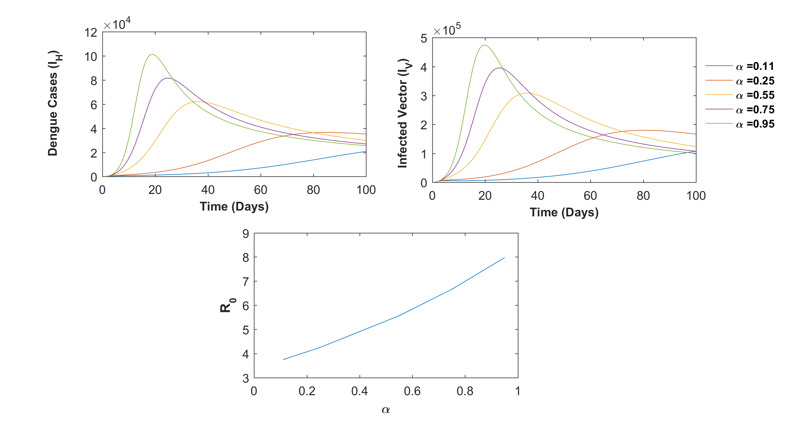
Figure 1: Effect of $\alpha$ (order of the fractional derivative in the force of infection occurring from infected vector to susceptible human) on the infected time-series (human and vector) of the dengue model (3.37) and on the basic reproduction number ($R_{0}$). Other parameters are taken from Table 2. Time step size ($h$) and the value of $\theta$ (see Appendix A for detail numerical scheme) to obtain a solution of the fractional order dengue model (3.37) are taken as $h=\frac{1}{5}$, and $\theta=\frac{1}{2}$, respectively.

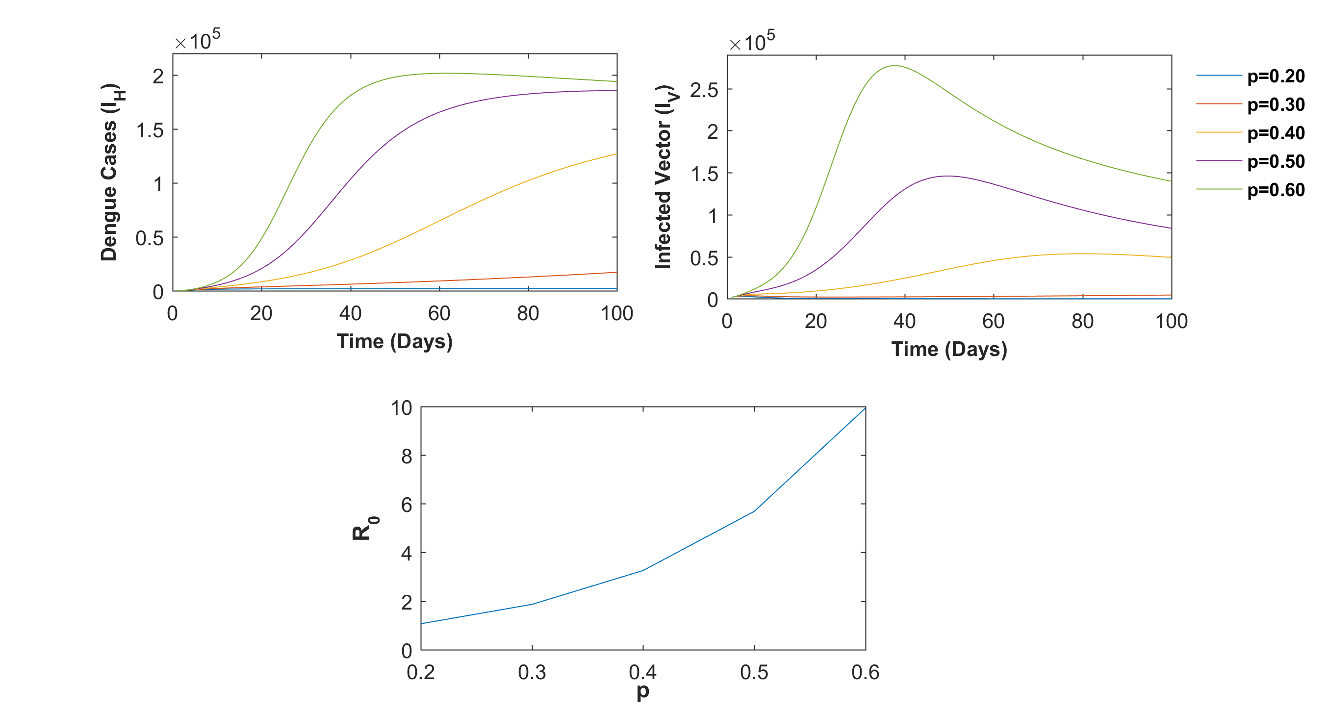
Figure 2: Effect of $p$ (order of the fractional derivative in the force of infection occurring from infected human to susceptible vector) on the infected time-series (human and vector) of the dengue model (3.37) and on the basic reproduction number ($R_{0}$). In this scenario, we take $\beta=0.15$ (as $0<\beta\leq p\leq 1$) and other parameters are taken from Table 2. Furthermore, we varies $p$ within the interval [0.20, 0.60] as in the dengue model (3.37), $p$ satisfies the relation $0<\beta\leq p\leq 1$. Time step size ($h$) and the value of $\theta$ (see Appendix A for detail numerical scheme) to obtain a solution of the fractional order dengue model (3.37) are taken as $h=\frac{1}{5}$, and $\theta=\frac{1}{2}$, respectively.

To see the effect of three fractional order parameters ($\alpha$, $\beta$, and $p$) on the time-series of the state-variables of the dengue model (3.37), we first vary $\alpha$, $\beta$, and $p$ within the interval $(0,1]$ and numerically solve the system (3.37) (see Fig 1 and Fig 2). We found that an increase in both $\alpha$ ($\alpha\to 1$) and $p$ ($p\to 1$) will increase the dengue (human and vector) epidemic peak and the total number of dengue cases in a region (see Fig 1 and Fig 2). Furthermore, we observed early dengue epidemic peak timings (the day at which epidemic peak occurs in a region) as $\alpha$ and $p$ are increased ($\alpha\to 1$, and $p\to 1$), respectively. These results are further established by the fact that an increase in both $\alpha$ ($\alpha\to 1$) and $p$ ($p\to 1$) will increase the basic reproduction number $R_{0}$ (see Fig 1 and Fig 2). Biologically, $\alpha$, and $p$ represent memory effects in disease transmission sardar2017mathematical ; du2013measuring . Thus, increasing the memory effect ($\alpha$ $\to$ 0, and $p$ $\to$ 0, respectively) in disease transmission may lead to longer epidemic duration and fewer dengue incidences in a region.

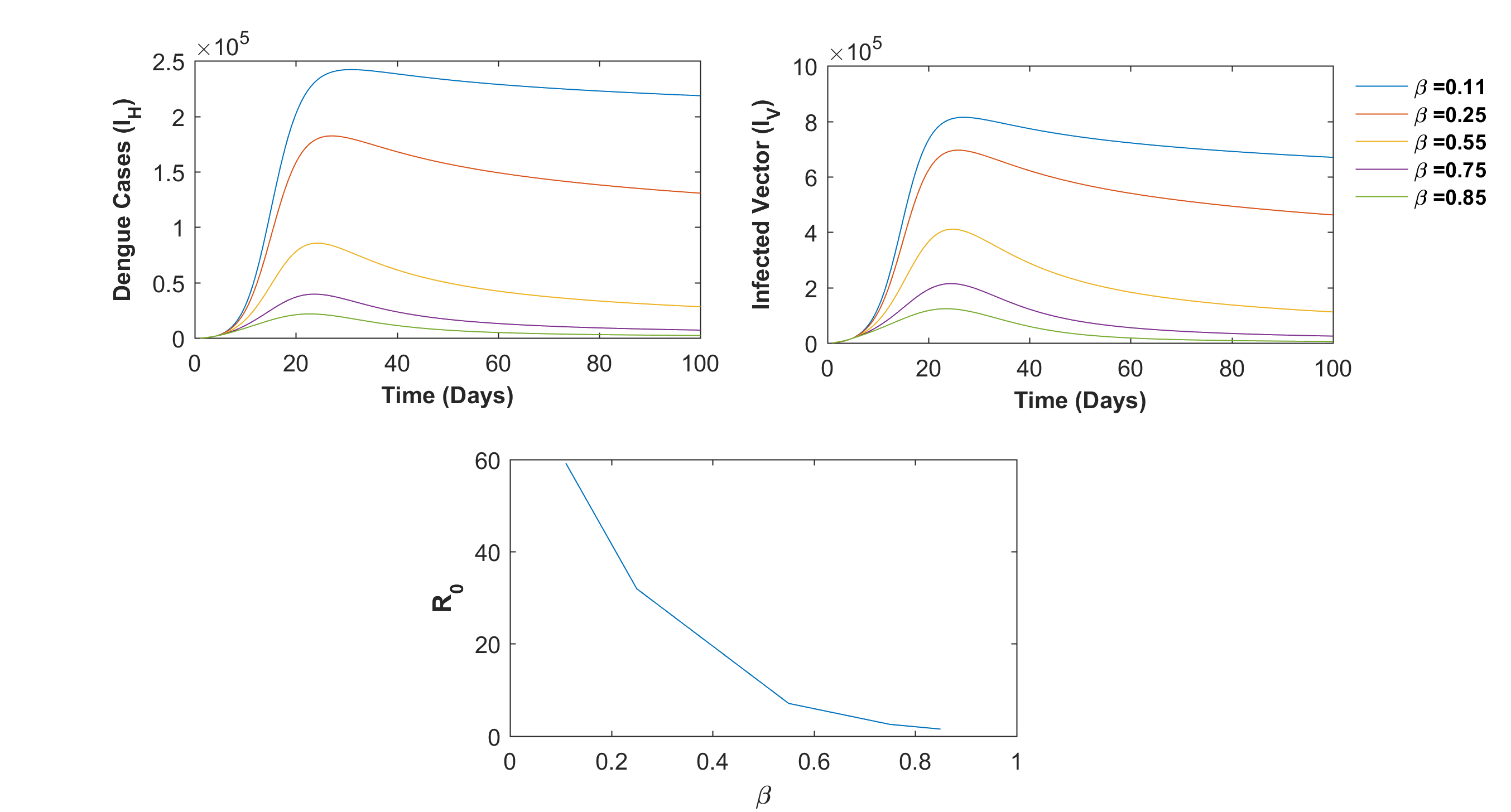
Figure 3: Effect of $\beta$ (order of the fractional derivative in the fractional order recovery term) on the infected time-series (human and vector) of the dengue model (3.37) and on the basic reproduction number ($R_{0}$). Other parameters are taken from Table 2. Moreover, we varies $\beta$ within the interval (0, 0.85] as in the dengue model (3.37), $\beta$ satisfies the relation $0<\beta\leq p\leq 1$. Time step size ($h$) and the value of $\theta$ (see Appendix A for detail numerical scheme) to obtain a solution of the fractional order dengue model (3.37) are taken as $h=\frac{1}{5}$, and $\theta=\frac{1}{2}$, respectively.

We found a different trend in case of varying fractional order recovery parameter $\beta$, as increasing $\beta$ ($\beta\to 1$) will decrease the dengue (human and vector) epidemic peak and the total number of dengue cases in a region (see Fig 3). This fact also established from the fact that $R_{0}$ has a negative correlation with $\beta$ (see Fig 3). However, in case of fractional order recovery parameter $\beta$, the epidemic peak timing remain unchanged as $\beta$ varies from 0 $\to$ 1 (see Fig 3). Epidemiologically, parameter $\beta$ represents a measure of the recovery rate of the infected human. Therefore, an increase in $\beta$ ($\beta$ $\to$ 1) may leads to faster recovery and subsequently, produce lesser number of dengue cases in a region.

We simultaneously solve the dengue state system (6.1) along with the co-state system (6.14) using forward-backward-sweep method lenhart2007optimal . Numerical discretization of the fractional derivatives appeared in both state system (6.1) and co-state system (6.14) are done using a implicit-$\theta$ scheme provided in Appendix A. Parameter values used in obtaining the numerical solution of dengue the control problem (6.2) are taken from Table 1 and Table 2.

We consider different control structures to reduce dengue epidemic in a location. Different control combination are provided below:

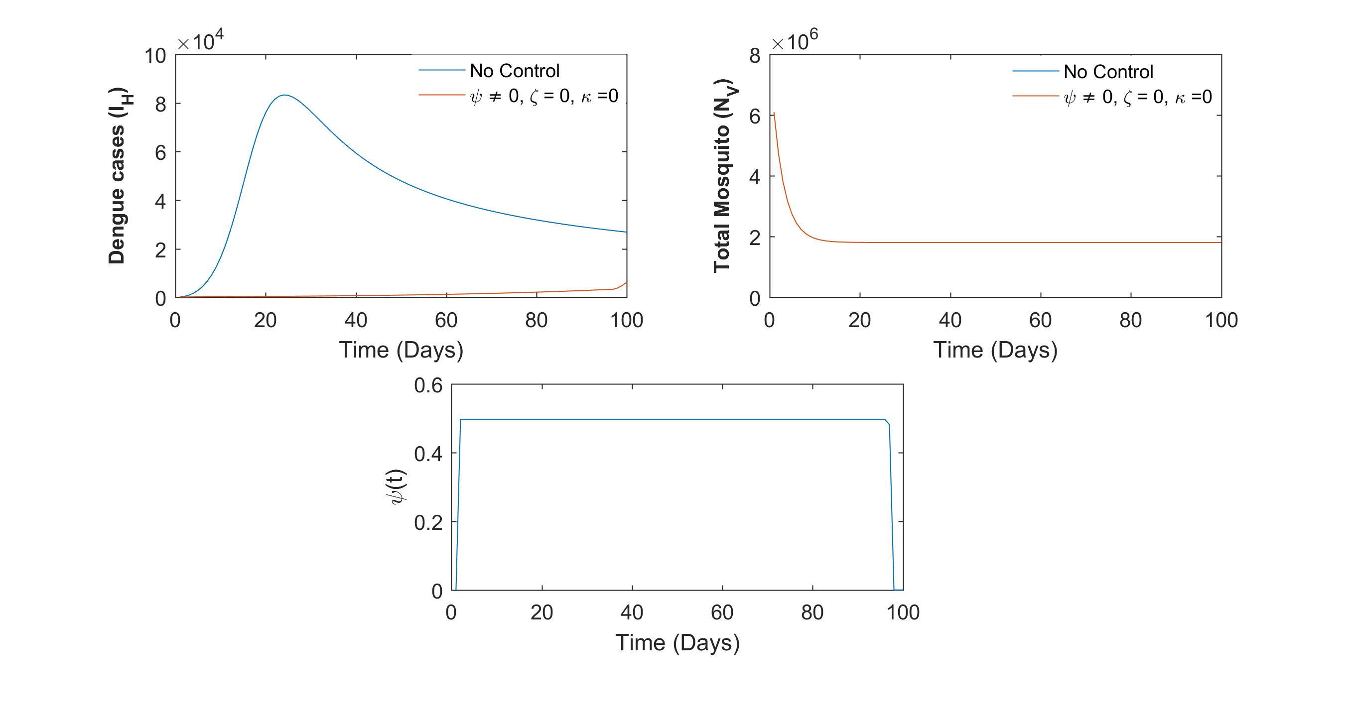
Figure 4: Optimal effect of only individual protection ($\psi(t)\neq 0$, $\zeta(t)=0$, $\kappa(t)=0$) like using mosquito net, mosquito repellent, etc. on dengue incidence in a region.

1. Individual precaution only ($S_{1}$): In this scenario, only individual protection (using mosquito net, mosquito repellent, etc.) is considered i.e. $\psi\neq 0$ and $\zeta=\kappa=0$. We found that applying this control may significantly reduce dengue cases in a location (see Fig. 4). However, the total mosquito population ($N_{V}$) may remain unchanged (see Fig. 4).

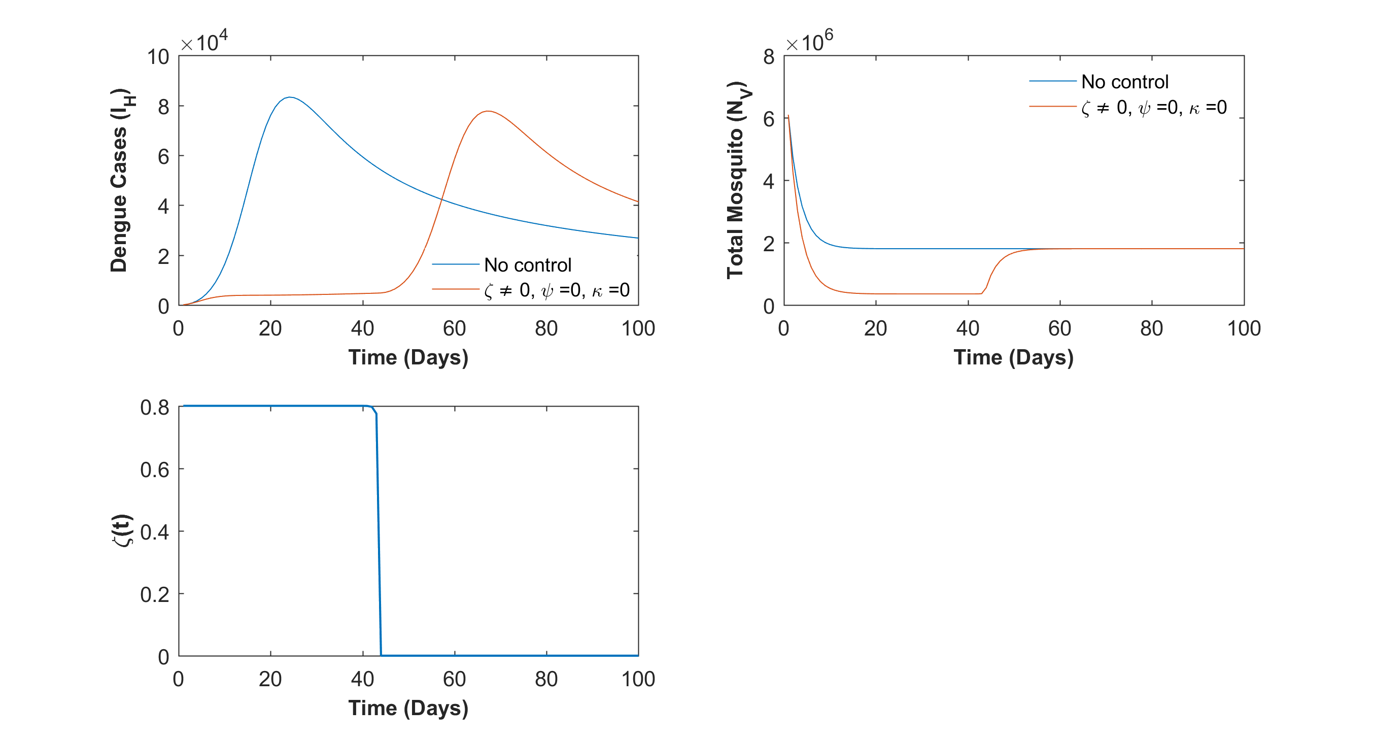
Figure 5: Optimal effect of reducing aquatic transition only ($\zeta(t)\neq 0$, $\psi(t)=0$, $\kappa(t)=0$) by spraying aquatic insecticides that kill mosquito egg, larvae, and pupae etc. on dengue incidence in a region.

2. Reducing aquatic transition only ($S_{2}$): In this control strategy, we considered reducing mosquito recruitment rate only (i.e. killing mosquito egg, larvae, and pupae by spraying aquatic insecticides, and therefore, it reduces aquatic transition rate) i.e. $\zeta\neq 0$, and $\psi=\kappa=0$. We found that applying this control dengue cases are reduced up to a certain time point but again cases increased when the effect of $\zeta$ is reduced (Fig. 5). Similar effect also be seen in case of total vector population $N_{V}$ (Fig. 5).

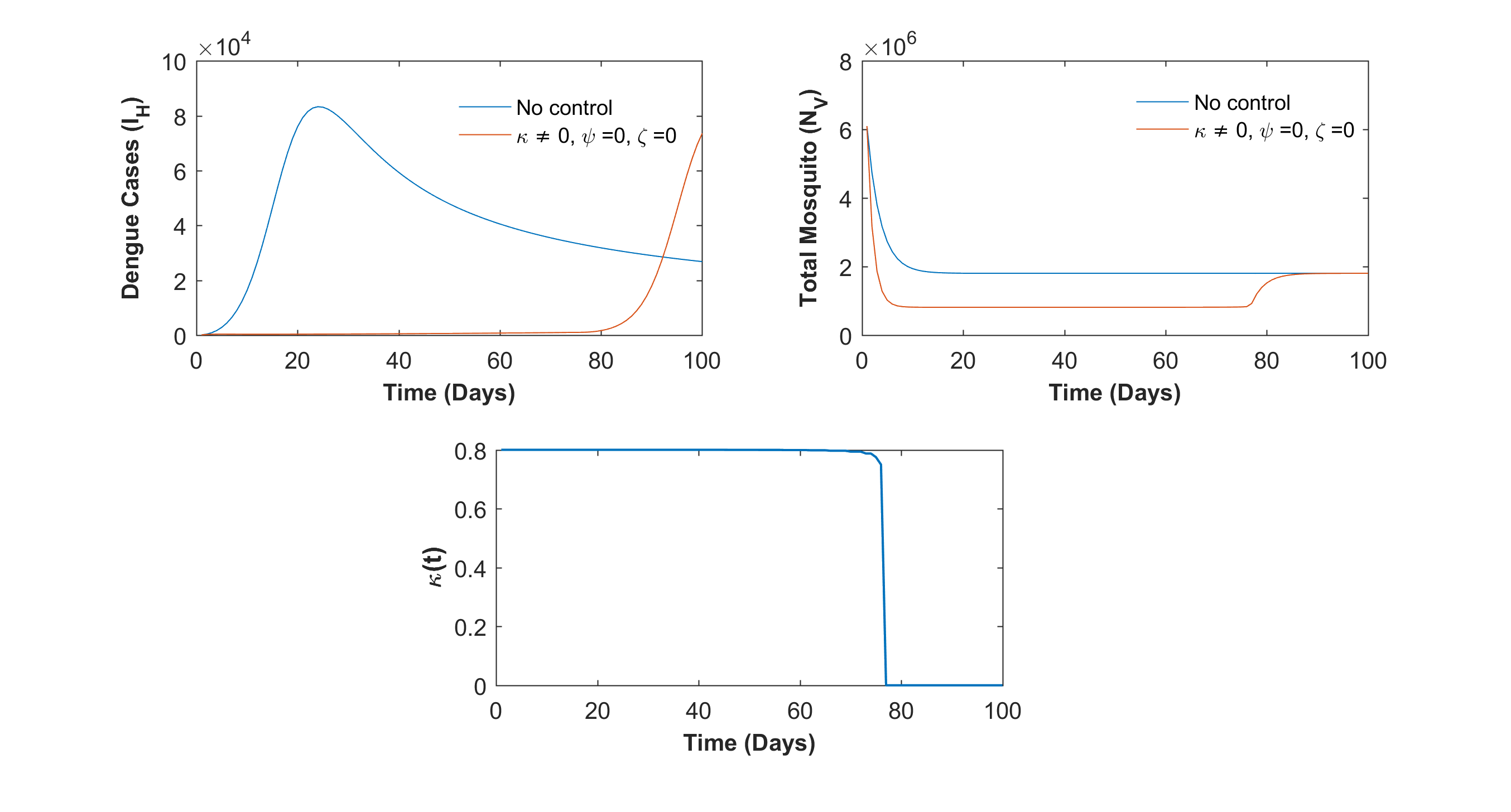
Figure 6: Optimal effect of reducing aquatic transition only ($\zeta(t)\neq 0$, $\psi(t)=0$, $\kappa(t)=0$) by spraying aquatic insecticides that kill mosquito egg, larvae, and pupae etc. on dengue incidence in a region.

3. Adult vector control only ($S_{3}$): In this control scenario, we considered adult vector control only (spraying adult insecticides) i.e. $\kappa\neq 0$, and $\psi=\zeta=0$. Applying this control, new dengue cases along with the total mosquito population reduced significantly (see Fig. 6).

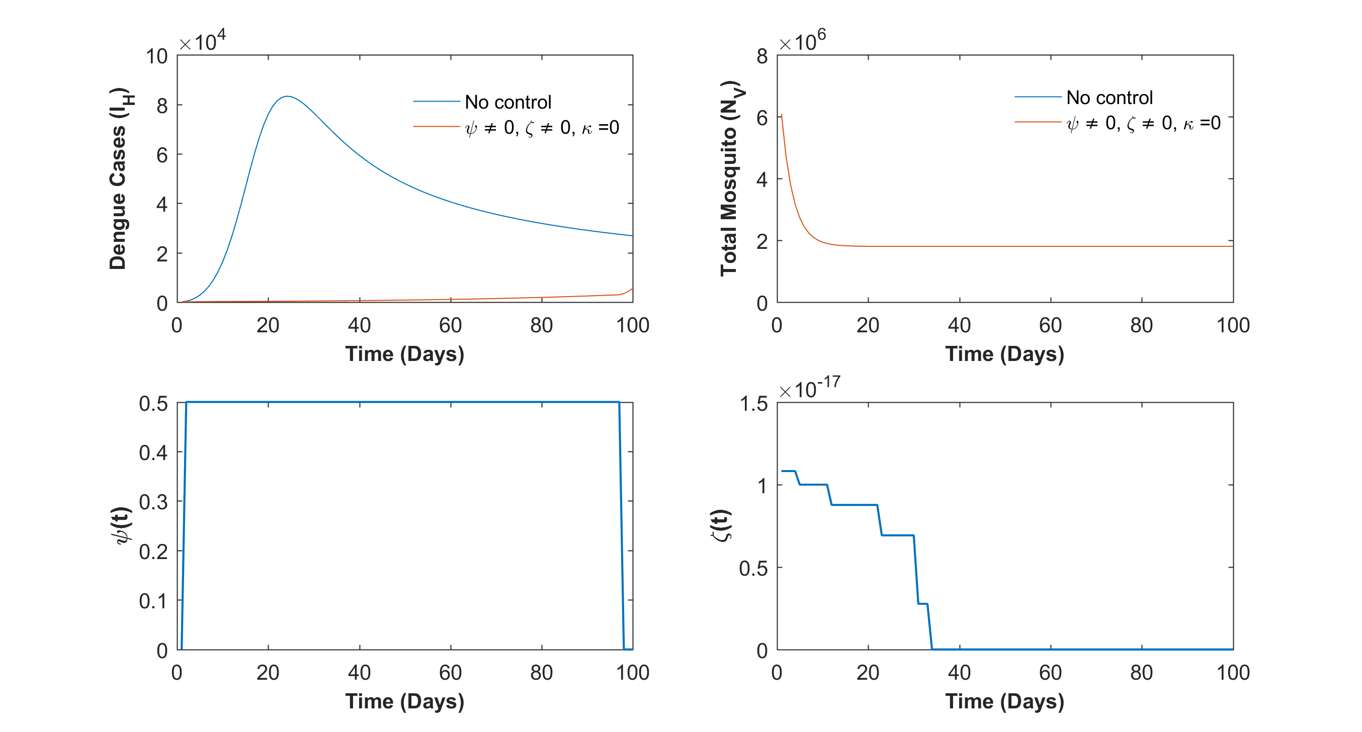
Figure 7: Optimal effect of the control combination namely individual protection and reduced aquatic transition ($\psi(t)\neq 0$, $\zeta(t)\neq 0$, $\kappa(t)=0$) on dengue epidemic in a region.

4. Individual precaution along with reduced aquatic transition ($S_{4}$): In this case, we considered combination of individual protection and aquatic transition control i.e. $\psi\neq 0$, $\zeta\neq 0$, and $\kappa=0$. In this scenario, we found that optimal effect of individual protection dominates aquatic transition as a result number of dengue cases reduce significantly but total mosquito population remain unchanged (see Fig. 7).

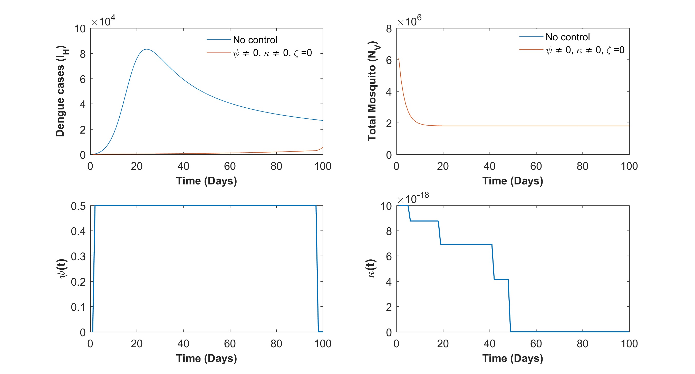
Figure 8: Optimal effect of the control combination namely individual protection and adult vector control ($\psi(t)\neq 0$, $\kappa(t)\neq 0$, $\zeta(t)=0$) on dengue epidemic in a region.

5. Individual precaution along with adult mosquito control ($S_{5}$): In this scenario, we considered combination of individual protection and adult vector control i.e. $\psi\neq 0$, $\kappa\neq 0$, and $\zeta=0$. As similar to previous case, in this control scenario also optimal effect $\psi$ dominates $\kappa$. Therefore, the number of dengue cases reduce significantly however total mosquito population remain unchanged (see Fig. 8).

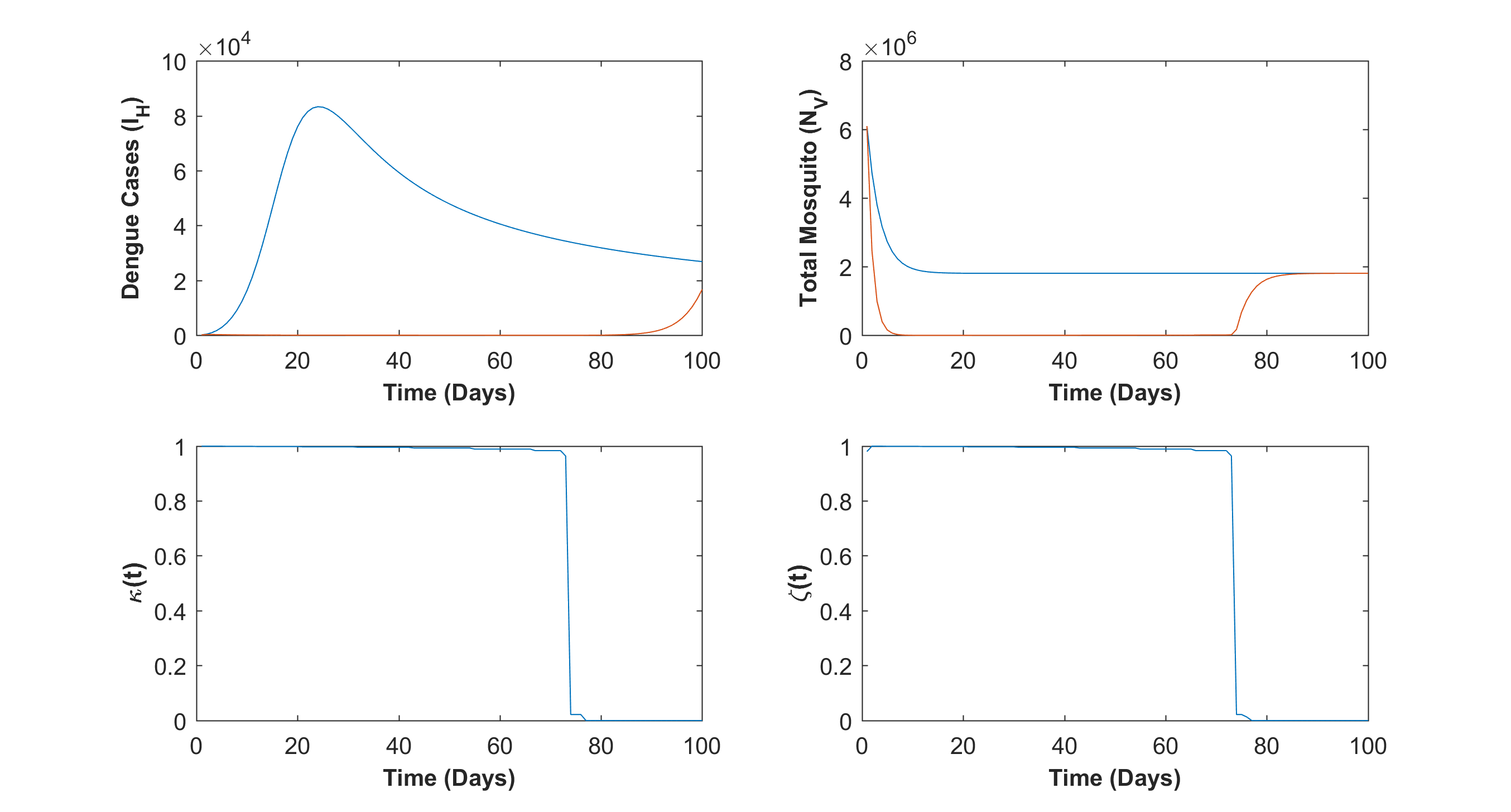
Figure 9: Optimal effect of the control combination namely adult vector control, and reduction in aquatic transition ($\kappa(t)\neq 0$, $\zeta(t)\neq 0$, $\psi(t)=0$) on dengue epidemic in a region.

6. Adult mosquito control along with reduction in aquatic transition ($S_{6}$): In this scenario, we considered combination of adult vector control and reduction in mosquito recruitment rate i.e. $\kappa\neq 0$, $\zeta\neq 0$, and $\psi=0$. We found that in this optimal control scenario the number of dengue cases as well as the total mosquito population are reduced significantly (see Fig. 9).

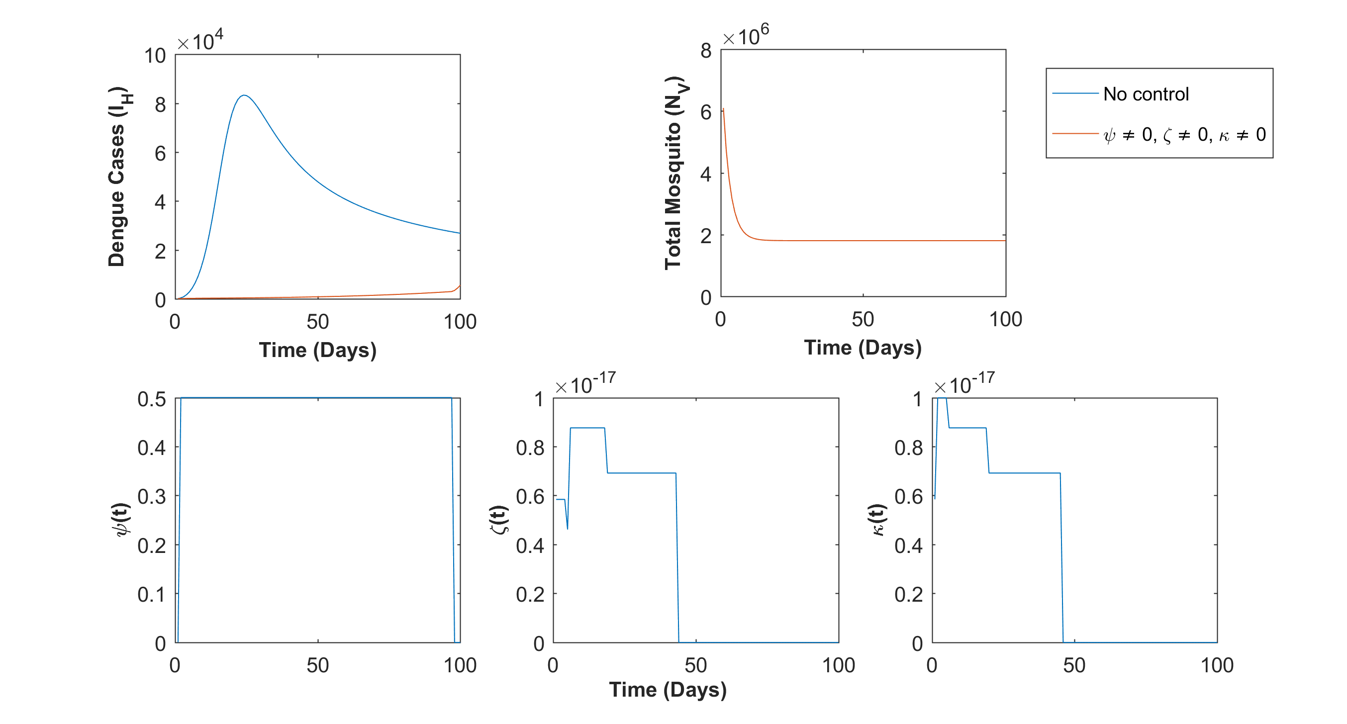
Figure 10: Optimal effect of all three control ($\psi(t)\neq 0$, $\kappa(t)\neq 0$, $\zeta(t)\neq 0$) on dengue epidemic in a region.

7. Combination of all control ($S_{7}$): In this scenario, we studied the optimal effect of all control ($\kappa\neq 0$, $\zeta\neq 0$, $\psi\neq 0$). In this case, optimal effect of individual protection dominates other two controls (adult vector control and reduction in mosquito recruitment rate). Therefore, optimal effect of all control reduce dengue cases significantly but total vector population remain unchanged (see Fig. 10).

7.1 Efficacy analysis

Now, we analyze the efficiency of different optimal combinations in terms of reducing the total number of dengue cases. We define efficacy index abboubakar2021mathematical as follows:

$$\displaystyle E_{I} =\displaystyle\left(1-\frac{\varepsilon^{c}}{\varepsilon^{0}}\right),$$ (7.1)

where, $\varepsilon^{c}$, and $\varepsilon^{0}$ are the cumulative number of dengue cases with control and without control, respectively. We computed $E_{I}$ for seven different control combinations mentioned previously (see Table 3). Our result on efficacy analysis suggest that the adult mosquito control in combination with the reduction in aquatic control ($S_{6}$) provide the best result in reducing cumulative number of dengue cases (see Table 3) in compare to other six control combinations.

Table 3: Efficacy of different optimal control combinations

Control Combination	$\varepsilon^{c}$	$E_{I}(\%)$
No control	4.27E6	0.00%
$S_{1}$	1.33E5	96.88%
$S_{2}$	2.94E6	31.16%
$S_{3}$	5.80E5	86.41%
$S_{4}$	1.22E5	97.13%
$S_{5}$	1.22E5	97.13%
$S_{6}$	7.37E4	98.27%
$S_{7}$	1.22E5	97.13%

8 Results and Discussion

Some recent studies indicate that some epidemic transmission and recovery processes may follow a non-Markovian distribution starnini2017equivalence ; lin2020non ; sherborne2018mean ; sardar2017mathematical ; sardar2015mathematical . To study more on this fact, we developed a new single-strain dengue model (3.37) with transmission and recovery processes following some power-law distribution. We showed that these power-law distributions in transmission and recovery processes lead to a fractional-order dengue system (3.37). In this new dengue model (3.37), fractional derivative appeared as tempered fractional derivative sabzikar2015tempered . Mathematically, we derived an approximation (see Theorem 2.1) of the tempered fractional derivative $\bigg{(}e^{-\beta t}\ _{RL}D_{t}^{\alpha}\left[e^{\beta t}F(t)\right]\approx\beta^{\alpha}F(t)\bigg{)}$ that appeared in the right hand side of the fractional order dengue system (3.37). We provide a mathematical proof of the positive invariance and the boundedness (see Proposition 2 and Proposition 3) of every forward solution of the fractional order dengue system (3.37). We derived the basic-reproduction number ($R_{0}$) for the fractional-order system (3.37), which is dependent on both transmission and recovery process parameters ($\alpha$, $\beta$, and $p$). The relationship between $R_{0}$ with $\alpha$, $\beta$, and $p$ are provided in Figures 1-to- 3. Moreover, we found that the fractional order dengue system (3.37) has a unique disease-free state ($\Psi_{0}$) and using the approximation provided in Theorem 2.1, we studied the local and global stability of $\Psi_{0}$ in terms of the basic reproduction number $R_{0}$ (see Proposition 4, and Proposition 5). Furthermore, we found that the fractional order dengue system (3.37) has a unique endemic equilibrium ($\Psi_{*}$) whenever $R_{0}>1$. Using poincaré-Bendixson theorem and a geometric framework li2002global , we prove the global stability of $\Psi_{*}$ in terms of $R_{0}$.

To study the effect of different interventions, we extended the dengue model (3.37) to a fractional order dengue model with control (6.1). Furthermore, we constructed an optimal control problem [see equation (6.2)] related to the fractional order dengue control system (6.1) to study the optimal effect of different dengue interventions in reducing the number of infected cases in a location. Furthermore, we state and proof (see Theorem 6.1) a sufficient condition for the existence of a solution to the optimal control problem related to the fractional order dengue control model (6.1).

As the analytical solution of the newly developed fractional-order dengue model (3.37) is almost impossible to be determined, therefore, we developed a numerical scheme (see Appendix 9) to study the dynamics of the dengue system (3.37). Furthermore, using this scheme, we also determined the solution of the optimal control problem [see section 6] related to the fractional order control model (6.1). Numerical findings suggest that increasing fractional order transmission parameters ($\alpha\to 1$, and $p\to 1$) will lead to faster epidemic growth (early peak timing and increasing $R_{0}$) and increase overall cases in a location (see Figures 1, and 2). As biologically, $\alpha$, and $p$ measure some memory effect in disease transmission du2013measuring ; saeedian2017memory ; sardar2017mathematical and therefore, increasing memory effect ($\alpha\to 0$, and $p\to 0$) in transmission process leads to slow epidemic peak timings. This result is in agreement with some previous studies on fractional-order transmission models sardar2017mathematical ; sardar2015mathematical . The power-law recovery process parameter $\beta$ does not have any effect on peak timing (see Figure 3). However, it may significantly change the cumulative dengue cases in a location (see Figure 3). Biologically, $\beta$ may represent a measure of recovery rate, and thus $\beta\to 1$ leads to a lower number of dengue incidences in a location (see Figure 3). Comparing the optimal effect of three dengue interventions and all their possible combinations suggests that adult mosquito control in combination with the reduction in aquatic transition may provide the best result in terms of dengue case reduction (see Figure 9, and Table 3). Thus, policymakers may focus on fractional-order transmission and recovery parameters ($\alpha$, $\beta$, $p$) along with vector controls (adult and aquatic) to reduce dengue transmission in a location.

Lastly, a few shortcomings of the current study can be noted, and they might be expanded upon in the future. There are evidences that asymptomatic and exposed cases of vector-borne diseases can transmit the disease to others duong2015asymptomatic ; gumel2012causes ; eshita2007vector ; wilder2004seroepidemiology . Incorporating these disease stages may lead to more complex results. We left this for future projects.

9 Appendix $A$. Numerical-Scheme

9.1 An implicit-$\theta$ method

To develop a numerical algorithm for the initial value problem (3.37), we used a one-step Euler method. We begin with the rectangle scheme to discretize the RL-fractional derivatives that appeared in the dengue model (3.37).

9.2 Rectangle method:

Let us assume that $[0,t_{max}]$ be the interval for which the problems (3.37) are well defined. We subdivide this interval into $(T+1)$ uniform grid by $t_{i}=ih,i=0,1,....T$, where, $h>0$, and $T=\left\lceil\frac{t_{max}}{h}\right\rceil$ is a positive integer. Furthermore, we assume that $S_{H}(i)=S_{H}(t_{i}),I_{H}(i)=I_{H}(t_{i}),R_{H}(i)=R_{H}(t_{i}),S_{V}(i)=S_{V}(t_{i}),I_{V}(i)=I_{V}(t_{i}),$ for $i=0,1....T$ are the approximation of $S_{H}$, $I_{H}$ and $I_{V}$ respectively at the point $t_{i}$. We approximate the system (3.37) as follows:

$$\frac{S_{H}(i+1)-S_{H}(i)}{h} =\mu_{H}N_{H}-\frac{b^{\alpha}}{N_{H}}\beta_{V}^{H}S_{H}(i+1)e^{-\mu_{V}(i+1)h}\leavevmode\nobreak\ _{RL}{D_{t}}^{1-\alpha}\left[I_{V}(t)e^{\mu_{V}t}\right]\Big{|}_{t=t_{i}}-\mu_{H}S_{H}(i+1)$$ (9.1)

$$\frac{I_{H}(i+1)-I_{H}(i)}{h} =\frac{b^{\alpha}}{N_{H}}\beta_{V}^{H}S_{H}(i+1)e^{-\mu_{V}(i+1)h}\leavevmode\nobreak\ _{RL}{D_{t}}^{1-\alpha}\left[I_{V}(t)e^{\mu_{V}t}\right]\Big{|}_{t=t_{i}}$$

$$-\frac{e^{-\mu_{H}(i+1)h}}{C^{\beta}}\leavevmode\nobreak\ _{RL}D_{t}^{1-\beta}\left[I_{H}(t)e^{\mu_{H}t}\right]\Big{|}_{t=t_{i}}-\mu_{H}I_{H}(i+1),$$

$$\frac{R_{H}(i+1)-R_{H}(i)}{h} =\frac{e^{-\mu_{H}(i+1)h}}{C^{\beta}}\leavevmode\nobreak\ _{RL}D_{t}^{1-\beta}\left[I_{H}(t)e^{\mu_{H}t}\right]\Big{|}_{t=t_{i}}-\mu_{H}R_{H}(i+1),$$

$$\frac{S_{V}(i+1)-S_{V}(i)}{h} =\Pi_{V}-\frac{b^{p}}{N_{H}C^{p}}\beta_{H}^{V}S_{V}(i+1)I_{H}(i+1)e^{-\mu_{H}(i+1)h}\leavevmode\nobreak\ _{RL}D_{t}^{1-p}\left[I_{H}(t)e^{\mu_{H}t}\right]\Big{|}_{t=t_{i}}-\mu_{V}S_{V}(i+1),$$

$$\frac{I_{V}(i+1)-I_{V}(i)}{h} =\frac{b^{p}}{N_{H}C^{p}}\beta_{H}^{V}S_{V}(i+1)I_{H}(i+1)e^{-\mu_{H}(i+1)h}\leavevmode\nobreak\ _{RL}D_{t}^{1-p}\left[I_{H}(t)e^{\mu_{H}t}\right]\Big{|}_{t=t_{i}}-\mu_{V}I_{V}(i+1),$$

We now determine an approximation of the fractional derivatives in the right-hand side of the system (3.37). From definition (2.2), we have:

$$_{RL}{D_{t}}^{1-\alpha}\Big{[}I_{V}(t)e^{\mu_{V}t}\Big{]} =\displaystyle\frac{1}{\Gamma(\alpha)}\frac{d}{dt}\int_{0}^{t}(t-\tau)^{\alpha-1}e^{\mu_{V}\tau}I_{V}(\tau)d\tau,$$ (9.2)

$$=\frac{1}{\Gamma(\alpha)}\frac{dH(t)}{dt},$$

where, $\displaystyle H(t)=\int_{0}^{t}(t-\tau)^{\alpha-1}e^{\mu_{V}\tau}I_{V}(\tau)d\tau$

Now using (9.2) we have ,

$$_{RL}{D_{t}}^{1-\alpha}\left[I_{V}(t)e^{\mu_{V}t}\right]\Big{|}_{t=t_{i}} =\frac{1}{\Gamma(\alpha)}\left[\frac{H(t_{i+1})-H(t_{i})}{h}\right]$$ (9.3)

$$=\frac{e^{\mu_{V}(i+1)h}}{h}\left[\sum_{j=0}^{i}\omega_{j,i}^{I_{V},R}I_{V}(t_{j+1})+e^{-\mu_{V}h}\sum_{j=0}^{i}\tilde{\omega}_{j,i}^{I_{V},R}I_{V}(t_{j+1})\right]$$

where,

$\omega_{j,i}^{I_{V},R}=\frac{1}{\mu_{V}^{\alpha}\Gamma(\alpha)}\left\{\begin{array}[]{ll}\gamma(\mu_{V}h,\alpha),&\mathrm{if}\text{ }(j=i)\\ \left[\gamma(\mu_{V}(i+1-j)h,\alpha)-\gamma(\mu_{V}(i-j)h,\alpha)\right]&\mathrm{if}\text{ }(j=0,1...(i-1))\\ \end{array}\right.\\$ $\tilde{\omega}_{j,i}^{I_{V},R}=\frac{1}{\mu_{V}^{\alpha}\Gamma(\alpha)}\left\{\begin{array}[]{ll}0,&\mathrm{if}\text{ }(j=i)\\ \left[\gamma(\mu_{V}(i-1-j)h,\alpha)-\gamma(\mu_{V}(i-j)h,\alpha)\right]&\mathrm{if}\text{ }(j=0,1...(i-1))\\ \end{array}\right.\\$

9.3 Trapezoidal method:

We use the piece-wise linear trapezoidal quadrature interpolation formula for the function given below:

$S_{H}(t)=\frac{t-t_{i+1}}{t_{i}-t_{i+1}}S_{H}(t_{i})+\frac{t-t_{i}}{t_{i+1}-t_{i}}S_{H}(t_{i+1})$,
$I_{H}(t)=\frac{t-t_{i+1}}{t_{i}-t_{i+1}}I_{H}(t_{i})+\frac{t-t_{i}}{t_{i+1}-t_{i}}I_{H}(t_{i+1})$,
$R_{H}(t)=\frac{t-t_{i+1}}{t_{i}-t_{i+1}}R_{H}(t_{i})+\frac{t-t_{i}}{t_{i+1}-t_{i}}R_{H}(t_{i+1})$,
$S_{V}(t)=\frac{t-t_{i+1}}{t_{i}-t_{i+1}}S_{V}(t_{i})+\frac{t-t_{i}}{t_{i+1}-t_{i}}S_{V}(t_{i+1})$,
$I_{V}(t)=\frac{t-t_{i+1}}{t_{i}-t_{i+1}}I_{V}(t_{i})+\frac{t-t_{i}}{t_{i+1}-t_{i}}I_{V}(t_{i+1}),$
for $i=0,1....T$ are the approximation of $S_{H},I_{H}$, and $I_{V}$ respectively at the point $t_{i}$ and $t_{i+1}$. Then approximate the term ${}_{RL}{D_{t}}^{1-\alpha}\left[M_{I}(t)e^{\mu_{m}t}\right]$ at $t=t_{i}$ as follows:

$$_{RL}{D_{t}}^{1-\alpha}\left[I_{V}(t)e^{\mu_{V}t}\right]\Big{|}_{t=t_{i}} =\frac{1}{\Gamma(\alpha)}\left[\frac{H(t_{i+1})-H(t_{i})}{h}\right]$$ (9.4)

$$=\frac{e^{\mu_{V}(i+1)h}}{h^{2}}\left[\sum_{j=0}^{i}\left(\omega_{j,i}^{I_{V},T}-e^{-\mu_{V}h}U_{j,i}^{I_{V},T}\right)I_{V}(t_{j})\right.$$

$$\left.\quad+\sum_{j=0}^{i}\left(\tilde{\omega}_{j,i}^{I_{V},T}-e^{-\mu_{V}h}\tilde{U}_{j,i}^{I_{V},T}\right)I_{V}(t_{j+1})\right]$$

where,

$\omega_{j,i}^{I_{V},T}=\frac{1}{\mu_{V}^{\alpha+1}\Gamma(\alpha)}\left\{\begin{array}[]{ll}\gamma(\mu_{V}h,\alpha+1),&\mathrm{if}\text{ }(j=i)\\ \left[\gamma(\mu_{V}(i+1-j)h,\alpha+1)-\gamma(\mu_{V}(i-j)h,\alpha+1)\right]\\ -\mu_{V}(i-j)h\left[\gamma(\mu_{V}(i+1-j)h,\alpha)-\gamma(\mu_{V}(i-j)h,\alpha)\right]&\mathrm{if}\text{ }(j=0,1...(i-1))\\ \end{array}\right.\\$ $U_{j,i}^{I_{V},T}=\frac{1}{\mu_{V}^{\alpha+1}\Gamma(\alpha)}\left\{\begin{array}[]{ll}0,&\mathrm{if}\text{ }(j=i)\\ \left[\gamma(\mu_{V}(i-j)h,\alpha+1)-\gamma(\mu_{V}(i-j-1)h,\alpha+1)\right]\\ -\mu_{V}(i-j-1)h\left[\gamma(\mu_{V}(i-j)h,\alpha)-\gamma(\mu_{V}(i-j-1)h,\alpha)\right]&\mathrm{if}\text{ }(j=0,1...(i-1))\\ \end{array}\right.\\$ $\tilde{\omega}_{j,i}^{I_{V}T}=\frac{1}{\mu_{V}^{\alpha+1}\Gamma(\alpha)}\left\{\begin{array}[]{ll}\mu_{V}h\gamma(\mu_{V}h,\alpha)-\gamma(\mu_{V}h,\alpha+1),&\mathrm{if}\text{ }(j=i)\\ \mu_{V}(i+1-j)h\left[\gamma(\mu_{V}(i+1-j)h,\alpha)-\gamma(\mu_{V}(i-j)h,\alpha)\right]\\ -\left[\gamma(\mu_{V}(i+1-j)h,\alpha+1)-\gamma(\mu_{V}(i-j)h,\alpha+1)\right]&\mathrm{if}\text{ }(j=0,1...(i-1))\\ \end{array}\right.\\$ $\tilde{U}_{j,i}^{I_{V}T}=\frac{1}{\mu_{V}^{\alpha+1}\Gamma(\alpha)}\left\{\begin{array}[]{ll}0,&\mathrm{if}\text{ }(j=i)\\ \mu_{V}(i-j)h\left[\gamma(\mu_{V}(i-j)h,\alpha)-\gamma(\mu_{V}(i-j-1)h,\alpha)\right]\\ -\left[\gamma(\mu_{V}(i-j)h,\alpha+1)-\gamma(\mu_{V}(i-j-1)h,\alpha+1)\right]&\mathrm{if}\text{ }(j=0,1...(i-1))\\ \end{array}\right.\\$

9.4 Implicit $\theta$-Method

Let the integral ${}_{RL}{D_{t}}^{1-\alpha}\left[y(t)e^{\mu_{m}t}\right]$ at $t=t_{i}$ can be discritize using $\theta-method$, which is defined as follows:

$${}_{RL}{D_{t}}^{1-\alpha}\left[y(t)e^{\mu_{m}t}\right]\Big{|}_{t=t_{i}} =\frac{e^{\mu_{m}(i+1)h}}{h}\left\{\theta\left[\sum_{j=0}^{i}\omega_{j,i}^{y,R}y(t_{j+1})+e^{-\mu_{m}h}\sum_{j=0}^{i}\tilde{\omega}_{j,i}^{y,R}y(t_{j+1})\right]\right.$$ (9.5)

$$\left.\quad+\frac{(1-\theta)}{h}\left[\sum_{j=0}^{i}\left(\omega_{j,i}^{y,T}-e^{-\mu_{m}h}U_{j,i}^{y,T}\right)y(t_{j})\right.\right.$$

$$\left.\left.\quad+\sum_{j=0}^{i}\left(\tilde{\omega}_{j,i}^{y,T}-e^{-\mu_{m}h}\tilde{U}_{j,i}^{y,T}\right)y(t_{j+1})\right]\right\}$$

where, we consider the $\theta-method$ as the combination of Rectangle and Trapezoidal method defined above (9.3) and (9.4). Then the differential equation $\frac{dy}{dt}=_{RL}{D_{t}}^{1-\alpha}\left[y(t)e^{\mu_{m}t}\right]$, can be discritize using Euler method as follows

$$y_{i+1} =y_{i}+\frac{e^{\mu_{m}(i+1)h}}{h}\left\{\theta\left[\sum_{j=0}^{i}\omega_{j,i}^{y,R}y(t_{j+1})+e^{-\mu_{m}h}\sum_{j=0}^{i}\tilde{\omega}_{j,i}^{y,R}y(t_{j+1})\right]\right.$$ (9.6)

$$\left.\quad+\frac{(1-\theta)}{h}\left[\sum_{j=0}^{i}\left(\omega_{j,i}^{y,T}-e^{-\mu_{m}h}U_{j,i}^{y,T}\right)y(t_{j})\right.\right.$$

$$\left.\left.\quad+\sum_{j=0}^{i}\left(\tilde{\omega}_{j,i}^{y,T}-e^{-\mu_{m}h}\tilde{U}_{j,i}^{y,T}\right)y(t_{j+1})\right]\right\}$$

.

Now, using (9.8) ${}_{RL}{D_{t}}^{1-\alpha}\left[I_{V}(t)e^{\mu_{V}t}\right]$ can be descritize as follows:

$${}_{RL}{D_{t}}^{1-\alpha}\left[I_{V}(t)e^{\mu_{V}t}\right]\Big{|}_{t=t_{i}} =\frac{e^{\mu_{V}(i+1)h}}{h}\left\{\theta\left[\sum_{j=0}^{i}\omega_{j,i}^{I_{V},R}I_{V}(t_{j+1})+e^{-\mu_{V}h}\sum_{j=0}^{i}\tilde{\omega}_{j,i}^{I_{V},R}I_{V}(t_{j+1})\right]\right.$$ (9.7)

$$\left.\quad+\frac{(1-\theta)}{h}\left[\sum_{j=0}^{i}\left(\omega_{j,i}^{I_{V},T}-e^{-\mu_{V}h}U_{j,i}^{I_{V},T}\right)I_{V}(t_{j})\right.\right.$$

$$\left.\left.\quad+\sum_{j=0}^{i}\left(\tilde{\omega}_{j,i}^{I_{V},T}-e^{-\mu_{V}h}\tilde{U}_{j,i}^{I_{V},T}\right)I_{V}(t_{j+1})\right]\right\}$$

Then the equation (9.1) can be transformed as system of equation:

$$\leavevmode\nobreak\ A_{S_{H}}S_{H}^{i+1,\theta}+B_{S_{H}}S_{H}^{i+1,\theta}I_{V}^{i+1,\theta}+C_{S_{H}}=0$$ (9.8)

$$A_{I_{H}}S_{H}^{i+1,\theta}+B_{I_{H}}I_{H}^{i+1,\theta}+C_{I_{H}}S_{H}^{i+1,\theta}I_{V}^{i+1,\theta}+D_{I_{H}}=0$$

$$A_{R_{H}}R_{H}^{i+1,\theta}+B_{R_{H}}I_{H}^{i+1,\theta}+C_{R_{H}}=0$$

$$A_{S_{V}}S_{V}^{i+1,\theta}+B_{S_{V}}S_{V}^{i+1,\theta}I_{H}^{i+1,\theta}+C_{S_{V}}=0$$

$$A_{I_{V}}S_{V}^{i+1,\theta}+B_{I_{V}}S_{V}^{i+1,\theta}I_{H}^{i+1,\theta}+C_{I_{V}}I_{V}^{i+1,\theta}+D_{I_{V}}=0$$

where,

$$A_{S_{H}} =1+\mu_{H}h$$ (9.9)

$$+\frac{b^{\alpha}}{N_{H}}\beta_{V}^{H}\left[\sum_{j=0}^{i-1}\left(\theta\left\{\omega_{j,i}^{I_{V},R}+e^{-\mu_{V}h}\tilde{\omega}_{j,i}^{I_{V},R}\right\}+\frac{(1-\theta)}{h}\sum_{j=0}^{i-1}\left(\tilde{\omega}_{j,i}^{I_{V},T}-e^{-\mu_{V}h}\tilde{U}_{j,i}^{I_{V},T}\right)\right)I_{V}(t_{j+1})\right.$$

$$\left.\quad+\frac{(1-\theta)}{h}\sum_{j=0}^{i}\left(\omega_{j,i}^{I_{V},T}-e^{-\mu_{V}h}U_{j,i}^{I_{V},T}\right)I_{V}(t_{j})\right]$$

$$B_{S_{H}} =\frac{b^{\alpha}}{N_{H}}\beta_{V}^{H}\left(\theta\left\{\omega_{i,i}^{I_{V},R}+e^{-\mu_{V}h}\tilde{\omega}_{i,i}^{I_{V},R}\right\}+\frac{(1-\theta)}{h}\left\{\tilde{\omega}_{i,i}^{I_{V},T}-e^{-\mu_{V}h}\tilde{U}_{i,i}^{I_{V},T}\right\}\right)$$

$$C_{S_{H}} =-S_{H}^{i,\theta}-h\mu_{H}N_{H}$$

$$A_{I_{H}} =1+h\mu_{H}-A_{S_{H}}$$ (9.10)

$$B_{I_{H}} =1+h\mu_{H}+\frac{1}{C^{\beta}}\left(\theta\left\{\omega_{i,i}^{I_{H},R}+e^{-\mu_{H}h}\tilde{\omega}_{i,i}^{I_{H},R}\right\}+\frac{(1-\theta)}{h}\left(\tilde{\omega}_{i,i}^{I_{H},T}-e^{-\mu_{H}h}\tilde{U}_{i,i}^{I_{H},T}\right)\right)$$

$$C_{I_{H}} =-B_{S_{H}}$$

$$D_{I_{H}} =-I_{H}^{i,\theta}+\frac{1}{C^{\beta}}\left[\sum_{j=0}^{i-1}\left(\theta\left\{\omega_{j,i}^{I_{H},R}+e^{-\mu_{H}h}\tilde{\omega}_{j,i}^{I_{H},R}\right\}+\frac{(1-\theta)}{h}\sum_{j=0}^{i-1}\left(\tilde{\omega}_{j,i}^{I_{H},T}-e^{-\mu_{H}h}\tilde{U}_{j,i}^{I_{H},T}\right)\right)I_{H}(t_{j+1})\right.$$

$$\left.\quad+\frac{(1-\theta)}{h}\sum_{j=0}^{i}\left(\omega_{j,i}^{I_{H},T}-e^{-\mu_{H}h}U_{j,i}^{I_{H},T}\right)I_{H}(t_{j})\right]$$

$$A_{R_{H}} =1+h\mu_{H}$$

$$B_{R_{H}} =1+h\mu_{H}-B_{I_{H}}$$

$$C_{R_{H}} =-R_{H}^{i,\theta}-D_{I_{H}}$$

$$A_{S_{V}} =1+\mu_{V}h$$

$$+\frac{b^{\alpha}\beta_{H}^{V}}{N_{H}C^{p}}\left[\sum_{j=0}^{i-1}\left(\theta\left\{\omega_{j,i}^{I_{H},R}+e^{-\mu_{H}h}\tilde{\omega}_{j,i}^{I_{H},R}\right\}+\frac{(1-\theta)}{h}\sum_{j=0}^{i-1}\left(\tilde{\omega}_{j,i}^{I_{H},T}-e^{-\mu_{H}h}\tilde{U}_{j,i}^{I_{H},T}\right)\right)I_{H}(t_{j+1})\right.$$

$$\left.\quad+\frac{(1-\theta)}{h}\sum_{j=0}^{i}\left(\omega_{j,i}^{I_{H},T}-e^{-\mu_{H}h}U_{j,i}^{I_{H},T}\right)I_{H}(t_{j})\right]$$

$$B_{S_{V}} =\frac{b^{\alpha}\beta_{H}^{V}}{N_{H}C^{p}}\left(\theta\left\{\omega_{i,i}^{I_{H},R}+e^{-\mu_{H}h}\tilde{\omega}_{i,i}^{I_{H},R}\right\}+\frac{(1-\theta)}{h}\left\{\tilde{\omega}_{i,i}^{I_{H},T}-e^{-\mu_{H}h}\tilde{U}_{i,i}^{I_{H},T}\right\}\right)$$

$$C_{S_{V}} =-S_{V}^{i,\theta}-h\Pi_{V}$$

$$A_{I_{V}} =1+h\mu_{V}-A_{S_{V}}$$

$$B_{I_{V}} =-B_{S_{V}}$$

$$C_{I_{V}} =1+h\mu_{V}$$

$$D_{I_{V}} =-I_{V}^{i,\theta}$$

10 Appendix $B$. Figures

References

- [1] W. H. Organization, “Dengue guidelines for diagnosis, treatment, prevention and control : new edition,” 2009.
- [2] D. J. Gubler and G. G. Clark, “Dengue/dengue hemorrhagic fever: the emergence of a global health problem.,” Emerging infectious diseases, vol. 1, no. 2, p. 55, 1995.
- [3] T. Sardar, S. Rana, and J. Chattopadhyay, “A mathematical model of dengue transmission with memory,” Communications in Nonlinear Science and Numerical Simulation, vol. 22, no. 1-3, pp. 511–525, 2015.
- [4] J. Ong, J. Aik, and L. C. Ng, “Adult aedes abundance and risk of dengue transmission,” PLoS Neglected Tropical Diseases, vol. 15, no. 6, p. e0009475, 2021.
- [5] S. Bhatt, P. W. Gething, O. J. Brady, J. P. Messina, A. W. Farlow, C. L. Moyes, J. M. Drake, J. S. Brownstein, A. G. Hoen, O. Sankoh, et al., “The global distribution and burden of dengue,” Nature, vol. 496, no. 7446, pp. 504–507, 2013.
- [6] T. P. Htun, Z. Xiong, and J. Pang, “Clinical signs and symptoms associated with who severe dengue classification: a systematic review and meta-analysis,” Emerging Microbes & Infections, vol. 10, no. 1, pp. 1116–1128, 2021.
- [7] D. J. Gubler, “Epidemic dengue/dengue hemorrhagic fever as a public health, social and economic problem in the 21st century,” Trends in microbiology, vol. 10, no. 2, pp. 100–103, 2002.
- [8] F. P. Pinheiro, S. J. Corber, et al., “Global situation of dengue and dengue haemorrhagic fever, and its emergence in the americas,” World health statistics quarterly, vol. 50, pp. 161–169, 1997.
- [9] M. Andraud, N. Hens, C. Marais, and P. Beutels, “Dynamic epidemiological models for dengue transmission: a systematic review of structural approaches,” PloS one, vol. 7, no. 11, p. e49085, 2012.
- [10] M. Aguiar, V. Anam, K. B. Blyuss, C. D. S. Estadilla, B. V. Guerrero, D. Knopoff, B. W. Kooi, A. K. Srivastav, V. Steindorf, and N. Stollenwerk, “Mathematical models for dengue fever epidemiology: A 10-year systematic review,” Physics of Life Reviews, vol. 40, pp. 65–92, 2022.
- [11] S. T. R. d. Pinho, C. P. Ferreira, L. Esteva, F. R. Barreto, V. Morato e Silva, and M. Teixeira, “Modelling the dynamics of dengue real epidemics,” Philosophical Transactions of the Royal Society A: Mathematical, Physical and Engineering Sciences, vol. 368, no. 1933, pp. 5679–5693, 2010.
- [12] R. P. Agarwal, S. K. Ntouyas, B. Ahmad, and M. S. Alhothuali, “Existence of solutions for integro-differential equations of fractional order with nonlocal three-point fractional boundary conditions,” Advances in Difference Equations, vol. 2013, no. 1, pp. 1–9, 2013.
- [13] I. Podlubny, “Fractional differential equations: an introduction to fractional derivatives, fractional differential equations, to methods of their solution and some of their applications,” 1999.
- [14] M. Du, Z. Wang, and H. Hu, “Measuring memory with the order of fractional derivative,” Scientific reports, vol. 3, no. 1, p. 3431, 2013.
- [15] A. Dokoumetzidis and P. Macheras, “Fractional kinetics in drug absorption and disposition processes,” Journal of pharmacokinetics and pharmacodynamics, vol. 36, no. 2, pp. 165–178, 2009.
- [16] A. Dokoumetzidis, R. Magin, and P. Macheras, “Fractional kinetics in multi-compartmental systems,” Journal of pharmacokinetics and pharmacodynamics, vol. 37, no. 5, pp. 507–524, 2010.
- [17] M. Saeedian, M. Khalighi, N. Azimi-Tafreshi, G. Jafari, and M. Ausloos, “Memory effects on epidemic evolution: The susceptible-infected-recovered epidemic model,” Physical Review E, vol. 95, no. 2, p. 022409, 2017.
- [18] M. Starnini, J. P. Gleeson, and M. Boguñá, “Equivalence between non-markovian and markovian dynamics in epidemic spreading processes,” Physical review letters, vol. 118, no. 12, p. 128301, 2017.
- [19] C. Angstmann, B. Henry, and A. McGann, “A fractional order recovery sir model from a stochastic process,” Bulletin of mathematical biology, vol. 78, no. 3, pp. 468–499, 2016.
- [20] T. Sardar and B. Saha, “Mathematical analysis of a power-law form time dependent vector-borne disease transmission model,” Mathematical biosciences, vol. 288, pp. 109–123, 2017.
- [21] C. N. Angstmann, B. I. Henry, and A. V. McGann, “A fractional-order infectivity and recovery sir model,” Fractal and Fractional, vol. 1, no. 1, p. 11, 2017.
- [22] C. N. Angstmann, A. M. Erickson, B. I. Henry, A. V. McGann, J. M. Murray, and J. A. Nichols, “A general framework for fractional order compartment models,” SIAM Review, vol. 63, no. 2, pp. 375–392, 2021.
- [23] Z. Wu, Y. Cai, Z. Wang, and W. Wang, “Global stability of a fractional order sis epidemic model,” Journal of Differential Equations, vol. 352, pp. 221–248, 2023.
- [24] Z.-H. Lin, M. Feng, M. Tang, Z. Liu, C. Xu, P. M. Hui, and Y.-C. Lai, “Non-markovian recovery makes complex networks more resilient against large-scale failures,” Nature communications, vol. 11, no. 1, p. 2490, 2020.
- [25] N. Sherborne, J. C. Miller, K. B. Blyuss, and I. Z. Kiss, “Mean-field models for non-markovian epidemics on networks,” Journal of mathematical biology, vol. 76, pp. 755–778, 2018.
- [26] C. N. Angstmann, B. I. Henry, and A. V. McGann, “A fractional-order infectivity sir model,” Physica A: Statistical Mechanics and its Applications, vol. 452, pp. 86–93, 2016.
- [27] R. Hilfer and L. Anton, “Fractional master equations and fractal time random walks,” Physical Review E, vol. 51, no. 2, p. R848, 1995.
- [28] X. Yang, L. Chen, and J. Chen, “Permanence and positive periodic solution for the single-species nonautonomous delay diffusive models,” Comput. Math. Appl., vol. 32, no. 4, pp. 109–116, 1996.
- [29] X.-Q. Zhao, Dynamical systems in population biology, vol. 16. Springer, 2003.
- [30] J. Watmough, “Reproduction numbers and sub-threshold endemic equilibria for compartmental models of disease transmission,” Mathematical biosciences, vol. 180, no. 1-2, pp. 29–48, 2002.
- [31] C. Castillo-Chavez, “On the computation of r. and its role on global stability carlos castillo-chavez*, zhilan feng, and wenzhang huang,” Mathematical approaches for emerging and reemerging infectious diseases: an introduction, vol. 1, p. 229, 2002.
- [32] M. Y. Li and J. S. Muldowney, “A geometric approach to global-stability problems,” SIAM Journal on Mathematical Analysis, vol. 27, no. 4, pp. 1070–1083, 1996.
- [33] M. Y. Li, J. R. Graef, L. Wang, and J. Karsai, “Global dynamics of a seir model with varying total population size,” Mathematical biosciences, vol. 160, no. 2, pp. 191–213, 1999.
- [34] M. Y. Li and L. Wang, “Global stability in some seir epidemic models,” in Mathematical approaches for emerging and reemerging infectious diseases: models, methods, and theory, pp. 295–311, Springer, 2002.
- [35] H. I. Freedman, S. Ruan, and M. Tang, “Uniform persistence and flows near a closed positively invariant set,” Journal of Dynamics and Differential Equations, vol. 6, pp. 583–600, 1994.
- [36] H. Smith, “Monotone dynamical systems,” Handbook of differential equations: ordinary differential equations, vol. 2, pp. 239–357, 2006.
- [37] H. Abboubakar, A. K. Guidzavai, J. Yangla, I. Damakoa, and R. Mouangue, “Mathematical modeling and projections of a vector-borne disease with optimal control strategies: A case study of the chikungunya in chad,” Chaos, Solitons & Fractals, vol. 150, p. 111197, 2021.
- [38] T. Sardar, S. Mukhopadhyay, A. R. Bhowmick, and J. Chattopadhyay, “An optimal cost effectiveness study on zimbabwe cholera seasonal data from 2008–2011,” PLoS One, vol. 8, no. 12, p. e81231, 2013.
- [39] W. H. Fleming and R. W. Rishel, Deterministic and stochastic optimal control, vol. 1. Springer Science & Business Media, 2012.
- [40] H. Gaff and E. Schaefer, “Optimal control applied to vaccination and treatment strategies for various epidemiological models,” Math. Biosci. Eng, vol. 6, no. 3, pp. 469–492, 2009.
- [41] V. Lakshmikantham, S. Leela, and A. A. Martynyuk, Stability analysis of nonlinear systems. Springer, 1989.
- [42] E. A. Coddington, An introduction to ordinary differential equations. Courier Corporation, 2012.
- [43] E. Coddington and N. Levinson, “Theory of ordinary differential equations (mcgraw-hill, new york, 1955).,” MR16: 1022b.
- [44] D. E. Kirk, Optimal control theory: an introduction. Courier Corporation, 2004.
- [45] S. Lenhart and J. T. Workman, Optimal control applied to biological models. CRC press, 2007.
- [46] F. Sabzikar, M. M. Meerschaert, and J. Chen, “Tempered fractional calculus,” Journal of Computational Physics, vol. 293, pp. 14–28, 2015.
- [47] V. Duong, L. Lambrechts, R. E. Paul, S. Ly, R. S. Lay, K. C. Long, R. Huy, A. Tarantola, T. W. Scott, A. Sakuntabhai, et al., “Asymptomatic humans transmit dengue virus to mosquitoes,” Proceedings of the National Academy of Sciences, vol. 112, no. 47, pp. 14688–14693, 2015.
- [48] A. B. Gumel, “Causes of backward bifurcations in some epidemiological models,” Journal of Mathematical Analysis and Applications, vol. 395, no. 1, pp. 355–365, 2012.
- [49] Y. Eshita, T. Takasaki, I. Takashima, N. Komalamisra, H. Ushijima, and I. Kurane, “Vector competence of japanese mosquitoes for dengue and west nile viruses,” Pesticide Chemistry: Crop Protection, Public Health, Environmental Safety, pp. 217–225, 2007.
- [50] A. Wilder-Smith, W. Foo, A. Earnest, S. Sremulanathan, and N. I. Paton, “Seroepidemiology of dengue in the adult population of singapore,” Tropical Medicine & International Health, vol. 9, no. 2, pp. 305–308, 2004.