Node-opening construction of maxfaces

Abstract.

The node-opening technique developed by Traizet has been very useful in constructing minimal surfaces. In this paper, we use the technique to construct families of maximal immersions in Lorentz space that are embedded outside a compact set. Each family depends on a real parameter $t$. The surfaces look like spacelike planes connected by small necks that shrink to singular points as $t\to 0$. The limit positions of the necks must satisfy a balance condition, which turns out to be exactly the same for maxfaces and for minimal surfaces. By simply comparing notes, we obtain a rich variety of new maxfaces with high genus and arbitrarily many space-like ends, including the Lorentzian Costa–Hoffman–Meeks surfaces, thereby remove the scarcity of examples of maxfaces. Moreover, a main task of this paper is to analyse the singularities, an interesting feature that distinguishes maxfaces from minimal surfaces. For sufficiently small non-zero $t$, the singular set consists of curves in the waist of every neck. In generic and some symmetric cases, we are able to prove that all but finitely many singularities are cuspidal edges, and the non-cuspidal singularities are swallowtails.

1. Introduction

Maximal surfaces are zero mean curvature immersions in the Lorentz Minkowski space ${\mathbb{E}}_{1}^{3}$. These surfaces emerge as solutions to the variational problem of locally maximizing the area among spacelike surfaces. They share several similarities with minimal surfaces in ${\mathbb{R}}^{3}$. For instance, both are critical points of the area functional and admit Weierstrass-Enneper representations. However, while there are rich examples of complete minimal surfaces, the only complete maximal immersion is the plane [umehara2006].

It is then natural to allow singularities. Following [imaizumi2008, lopez2007, umehara2006], etc., we adopt the term maximal map for maximal immersions with singularities. A maximal map is called a maxface if its singularities consist solely of points where the limiting tangent plane contains a light-like vector [umehara2006]. Umehara and Yamada also defined completeness for maxfaces [umehara2006]. Complete non-planar maxfaces always possess a compact singularity set. At the singularities, a maxface cannot be embedded, regardless of whether the rest of the surface is embedded. Therefore, following [fujimori2009, kim2006, umehara2006], we adopt embeddedness in wider sense as follows:

Definition 1.1.

A complete maxface is embedded in a wider sense if it is embedded outside of some compact subset.

Now that singularities are allowed, there are many examples of complete maxfaces, such as the Lorentzian Catenoid and Kim-Yang Toroidal maxface [kim2006]. In 2006, Kim and Yang [kim2006] constructed complete maximal maps of genus $k\geq 1$. When $k=1$, it is a complete embedded (in a wider sense) maxface known as Kim-Yang toroidal maxface. When $k>1$, they are not maxfaces. In [fujimori2009], the authors constructed a family of complete maxfaces $f_{k}$ for $k\geq 1$ with two ends; but when $k>1$, these may not be embedded (in a wider sense). Moreover, in 2016, Fujimori, Mohamed, and Pember [fujimori2016h] constructed maxfaces of any odd genus $g$ with two complete ends (if $g=1$, the ends are embedded) and maxfaces of genus $g=1$ and three complete embedded ends.

There is a scarcity of examples of complete maxfaces [fujimori2009]. All higher-genus maxfaces in the literature, to our best knowledge, have only two or three ends, usually of the catenoid type. Very few known higher-genus maxfaces are embedded (in a wider sense). Open problems in [fujimori2009] expressed hope for a large collection of examples of complete maxfaces that are embedded (in a wider sense) with higher genus and many ends.

In this paper, we construct a rich variety of complete maxfaces that are embedded (in a wider sense) of high genus and arbitrary number of spacelike ends. Each of these families depends on a sufficiently small non-zero real parameter $t$.

Our primary tool of construction will be the node opening technique, a Weierstrass gluing method developed by Traizet [traizet2002e]. The approach starts from Weierstrass data defined on a Riemann surface with nodes, then obtains Riemann surfaces by opening the nodes into necks and, at the same time, extends the Weierstrass data to Riemann surfaces using the Implicit Function Theorem. The node-opening technique has been very successful in constructing a rich variety of minimal surfaces [traizet2002e]. However, to the best of our knowledge, the current paper marks the first application of the technique to surfaces in the Lorentz-Minkowski space.

The Weierstrass gluing method has several advantages over other methods. On the one hand, in the existing literature on maxfaces, authors often need to assume symmetries to make the construction possible, hence only produce examples restricted to symmetries. The gluing technique has been a very powerful tool to break symmetries in minimal surfaces; in some sense, the technique was developed for this purpose [traizet2002e]. We will see later that it is equally powerful in breaking symmetries for maximal surfaces, hence ideal for removing the scarcity of examples. On the other hand, while the PDE gluing method is also popular for constructing minimal surfaces, the existence of singularities makes it difficult to apply on maxfaces. More specifically, one needs to identify (glue) two curves in the process, but the analysis would be difficult if the curves contain singularities. In the Weierstrass gluing process, we instead identify (glue) two annuli; hence, we can bypass the singularities.

The node-opening construction for maxfaces turns out to be very similar to that for minimal surfaces, hence will only be sketched in Section 4. This similarity implies that, for any minimal surface constructed by opening nodes, there is a corresponding maxface also constructed by opening nodes. This correspondence between maximal and minimal immersions is different from the usual correspondence through Weierstrass data [umehara2006]. Then in Section 3, by simply comparing notes, we obtain a rich variety of new maxfaces with high genus and arbitrarily many space-like ends, thereby remove the scarcity of examples of maxfaces. Among the examples are the Lorentzian Costa and Costa–Hoffman–Meeks (CHM) surfaces and their generalizations with arbitrarily many ends, providing positive answers to the open problems in [fujimori2009]. To the best of our knowledges, these are the first time that Lorentzian analogues of CHM surfaces were constructed.

Remark 1.2.

One could also use the node-opening technique to glue catenoids into periodic maxfaces, even of infinite genus, just by mimicking [traizet2002r, traizet2008t, morabito2012, chen2021, chen2023]. We believe that many examples in the existing literature, e.g. Lorentzian Riemann examples and Schwarz P surfaces, etc, can be produced in this way [fujimori2009, lopez2000m]. However, we do not plan to implement such constructions.

The singularity structure is an interesting feature that is special for maxfaces. Complete non-planar maxfaces always appear with singularities, such as cuspidal edges, swallowtails, cuspidal crosscaps, and cone-like singularities, to name a few. We refer the readers to [umehara2006, sai2022, kumar2020] to explore various singularities on maxfaces. In Section 5, we will analyse the types of singularities on the maxfaces that we construct using their Weierstrass data.

Components of the singular set are waists around the necks. We first prove in Theorem 5.1 that, around a specific neck and for sufficiently small non-zero $t$, either the singular set is mapped to a single point (cone-like singularity), or all but finitely many singular points are cuspidal edges. Moreover, the finitely many non-cuspidal singularities are generalized $A_{k}$ singularities, their positions on the waist depend analytically on $t$, and their types do not vary for sufficiently small $t$. Then, in Proposition 5.2, we show that, generically, there are four swallowtail singularities around a neck. The non-generic cases are generally hard to study. But in Section 5.5, we managed to analyse the singularities in the presence of rotational and reflectional symmetries. In Section 3, we will use the Lorentzian Costa and Costa–Hoffman–Meeks surfaces to examplify our results on singularities.

Acknowledgment

The first and third authors would like to extend their sincere gratitude to Professor S. D. Yang for graciously inviting them to The 3rd Conference on Surfaces, Analysis, and Numerics at Korea University. They are truly grateful for the opportunity, and our current work has commenced.

2. Main results

We want to construct maxfaces that look like horizontal (spacelike) planes connected by small necks. For that, we consider $L$ horizontal planes, labeled by integers $l\in[1,L]$. We want $n_{l}>0$ necks at level $l$, that is, between the planes $l$ and $l+1$, $1\leq l<L$. For convenience, we adopt the convention that $n_{0}=n_{L}=0$, and write $N=\sum n_{l}$ for the total number of necks. Each neck is then labeled by a pair $(l,k)$ with $1\leq l<L$ and $1\leq k\leq n_{l}$.

To each plane is associated a real number $Q_{l}$, indicating the logarithmic growth of the catenoid ($Q_{l}\neq 0$) or planar ends ($Q_{l}=0$). To each neck is associated a complex number $p_{l,k}\in{\mathbb{C}}$ indicating its horizontal limit position at $t=0$. We write $p=(p_{l,k})_{1\leq l<L,1\leq k\leq n_{l}}$ and $Q=(Q_{l})_{1\leq l<L}$. The pair $(p,Q)$ is called a configuration.

Given a configuration $(p,Q)$, let $c_{l}$ be the real numbers that solve

$$Q_{l}=n_{l-1}c_{l-1}-n_{l}c_{l},\qquad 1\leq l\leq L,$$

under the convention that $c_{0}=c_{L}=0$. A summation over $l$ yields that $\sum Q_{l}=0$, which is necessary for $c=(c_{l})_{1\leq l\leq L}$ to be uniquely determined as a linear function of $Q$. In fact, we may even replace $Q$ by $c$ in the definition of a configuration. Geometrically, $c_{l}$ corresponds to the “size” of the necks at level $l$.

For the neck $(l,k)$ in a configuration, we define the force $F_{l,k}$ on the neck as

$$F_{l,k}=\sum_{1\leq i\neq k\leq n_{l}}\frac{2c_{l}^{2}}{p_{l,k}-p_{l,i}}-\sum_{i=1}^{n_{l+1}}\frac{c_{l}c_{l+1}}{p_{l,k}-p_{l+1,i}}-\sum_{i=1}^{n_{l-1}}\frac{c_{l}c_{l-1}}{p_{l,k}-p_{l-1,i}}.$$

Note that we have necessarily $\sum F_{l,k}=0$.

Alternatively, let

$${\omega}_{l}=-\sum_{k=1}^{n_{l}}\frac{c_{l}\;dz}{z-p_{l,k}}+\sum_{i=1}^{n_{l-1}}\frac{c_{l-1}\;dz}{z-p_{l-1,k}}$$

be the unique meromorphic $1$-form on ${\mathbb{C}}_{l}$ with simple poles at $p_{l,k}$ and $p_{l-1,k}$, respectively with residues $-c_{l}$ and $c_{l-1}$. Then, the force is given by

$$F_{l,k}=\frac{1}{2}\operatorname{Res}_{p_{l,k}}\left(\frac{\omega_{l}^{2}}{dz}+\frac{\omega_{l+1}^{2}}{dz}\right).$$

Definition 2.1.

A configuration is balanced if $F_{l,k}=0$ for all $1\leq l<L$ and $1\leq k\leq n_{l}$, and is rigid if the differential of $F=(F_{l,k})_{1\leq l<L,1\leq k\leq n_{l}}$ with respect to $p$ has a complex rank of $n-2$.

In fact, $n-2$ is the maximum possible rank. To see this, note that the forces $F$ are invariant under the translations and complex scalings of $p$.

A necessary condition for the balance is

$$W:=\sum_{l=1}^{L}\sum_{k=1}^{n_{l}}p_{l,k}F_{l,k}=\sum_{l=1}^{L-1}n_{l}(n_{l}-1)c_{l}^{2}-\sum_{l=1}^{L-2}n_{l}n_{l+1}c_{l}c_{l+1}=0.$$

We now state our main result.

Theorem 2.2.

Let $(p,Q)$ be a balanced and rigid configuration such that the differential of $Q\mapsto W$ has rank $1$. Then, for sufficiently small $t$, there is a smooth family $M_{t}$ of complete maxfaces with the following asymptotic behaviors as $t\to 0$

• The maxfaces are of genus $N-L+1$ with $L$ space like ends, whose logarithmic growths converge to $Q_{l}$.

• After suitable scalings, the necks at level $l$ converge to Lorentzian catenoids;

• $M_{t}$ scaled by $t$ converges to an $L$-sheeted space-like plane with singular points at $p_{l,k}$.

Moreover, $M_{t}$ is embedded in a wider sense for sufficiently small $t$ if $Q_{1}<Q_{2}<\cdots<Q_{L}$.

To state our result on singularities, we need to define

(2.1) $$R^{(r)}_{l,k}(\theta)=\begin{dcases}\operatorname{Im}\bigg{(}e^{(r+1)i\theta}\overline{\operatorname{Res}_{p_{l,k}}\frac{\omega_{l}^{r+2}}{dz}}-e^{-(r+1)i\theta}\operatorname{Res}_{p_{l,k}}\frac{\omega_{l+1}^{r+2}}{dz}\bigg{)},&l\text{ odd},\\ \operatorname{Im}\bigg{(}e^{(r+1)i\theta}\operatorname{Res}_{p_{l,k}}\frac{\omega_{l}^{r+2}}{dz}-e^{-(r+1)i\theta}\overline{\operatorname{Res}_{p_{l,k}}\frac{\omega_{l+1}^{r+2}}{dz}}\bigg{)},&l\text{ even}.\end{dcases}$$

Our results about singularities are summarized below.

Theorem (Informal).

On a maxfaces constructed above, for sufficiently small non-zero $t$,

• The singular set has $N$ singular components, each being a curve around the waist of a neck.

• The singularities are all nondegenerate.

• If the singular curve is not mapped to a single point (cone-like singularity), then all but finitely many singular points are cuspidal edges.

• The non-cuspidal singularities are generalized $A_{k}$ singularities, their positions vary analytically with $t$, and their types do not vary.

• If $R^{(1)}_{l,k}\neq 0$, then there are exactly four non-cuspidal singularities around the neck $(l,k)$, and they are all swallowtails. Moreover, they tend to be evenly distributed on the waist as $t\to 0$.

The results above cover the generic situations. The non-generic cases are hard to analyze. However, if the configuration has symmetries, we have the following results:

1. Assume that the configuration has rotational symmetry of order $r>1$s around a neck and $R^{(r-1)}_{l,k}\neq 0$, then for sufficiently small non-zero $t$, there are $2r$ swallowtail singularities around the neck, and they tend to be evenly distributed as $t\to 0$.

2. Assume that the configuration has a vertical reflection plane that cuts through a neck, then the singularity around the neck that is fixed by the reflection is non-cuspidal.

3. Assume that the configuration of necks has a horizontal reflection plane that cuts through a neck, then the singular curve around the neck is mapped to a conelike singularity.

We will demonstrate these situations by examples in the next section.

Remark 2.3.

Because the singularities are all non-degenerate for sufficiently small $t$, we do not have any cuspidal cross caps. However, if we glue Lorentzian helicoids into maxfaces (see [traizet2005, freese2022, chen2022] for constructions of minimal surfaces), then by the duality between swallowtails and cuspidal cross caps [fujimori2008], we would expect no swallowtails but only cuspidal cross caps.

3. Examples

3.1. Configurations from minimal surfaces

Note that the balance and non-degeneracy conditions are exactly the same for maxfaces and for minimal surfaces. So all the configurations found in [traizet2002e] that give rise to the minimal surface also give rise to maxfaces. We now summarize some balanced and non-degenerate configurations (or methods to produce configurations) from [traizet2002e], and the corresponding maxfaces.

• The simplest configuration would have a single neck, given by

  $$L=2,\quad n_{1}=1,\quad p_{1,1}=0,$$

  $$Q_{1}=-1,\quad Q_{2}=1,\quad(\text{so }c_{1}=1).$$

  The corresponding maxface is the Lorentzian catenoid. It is of genus $0$, has two spacelike ends.

• The Costa–Hoffman–Meeks (CHM) configurations are given by

  $$L=3,\quad n_{1}=1,\quad n_{2}=m,$$

  $$p_{1,1}=0,\quad p_{2,m}=e^{2k\pi i/m},\quad 1\leq k\leq m,$$

  $$Q_{1}=1-m,\quad Q_{2}=-1,\quad Q_{3}=m\quad(\text{so }c_{1}=m-1,\quad c_{2}=1).$$

  We call the corresponding maxfaces Lorentzian Costa ($m=2$) or Costa–Hoffman–Meeks (CHM) surfaces ($m>2$). They provide positive answers to Problem 1 in [fujimori2009].

  Theorem 3.1.

  For each $g>1$, there exist complete embedded (in a wider sense) maxfaces with $3$ spacelike ends and genus $g$.

• Dihedral configurations with arbitrary number of ends were explicitly constructed in [traizet2008n]. They are given by $n_{1}=1$ and $n_{2}=\ldots n_{L-1}=m$, subject to a dihedral symmetry of order $m$. These configurations are balanced, and non-degenerate for a generic choice of $c_{l}$. The embeddedness condition $Q_{1}<\cdots<Q_{L}$ is satisfied if $m>2(L-2)$. Taking $m=2L-3$, we obtain generalizations of CHM maxfaces that provide positive answer to Problem 2 in [fujimori2009].

  Theorem 3.2.

  For each $L>3$, there exist complete embedded (in a wider sense) maxfaces with $L$ spacelike ends and genus $2(L-2)^{2}$.

• Numerical examples can be obtained by the polynomial method. More specifically, let

  $$P_{l}=\prod_{k=1}^{n_{l}}(z-p_{l,k}),\quad P=\prod_{l=1}^{L-1}P_{l},$$

  then the configuration is balanced if

  $$\sum_{l=1}^{L-1}c_{l}^{2}P\frac{P^{\prime\prime}_{l}}{P_{l}}-\sum_{l=1}^{L-2}c_{l}c_{l+1}P\frac{P^{\prime}_{l}P^{\prime}_{l+1}}{P_{l}P_{l+1}}\equiv 0.$$

  If a polynomial solution to this differential equation has only simple roots, then the roots correspond to the positions of nodes (up to permutations).

• Implicit examples can be obtained by perturbing “singular” configurations.

  More specifically, consider a partition $I_{1},...,I_{m}$ of the nodes and a family of configurations given by $p_{l,k}^{\lambda}=\hat{p}_{\mu}+\lambda_{\mu}\tilde{p}_{l,k,\mu}$ when $(l,k)\in I_{\mu}$. Then, the limit configuration $p^{0}$ is singular. A force can be defined for the limit configuration in terms of $\hat{p}$ and the partition. For each $\mu$, $\tilde{p}_{l,k,\mu}$ form a subconfiguration $\tilde{p}_{\mu}$.

  In the backward direction, Traizet [traizet2002e] found sufficient conditions to recover configuration $p^{\lambda}$ from the limit configuration $\hat{p}$ and the sub-configurations $\tilde{p}_{\mu}$. In particular, the limit configuration and all sub-configurations should be balanced. This result was used to construct examples with no symmetry. Using exactly the same configuration, we also obtain

  Theorem 3.3.

  There exist complete embedded (in a wider sense) maxfaces with no nontrivial symmetries.

Remark 3.4.

As we have noticed in Remark 1.2, a similar technique can produce periodic maxfaces. Although we do not plan to implement such constructions, it is predictable that the balance and non-degeneracy conditions are again the same for maxfaces and for minimal surfaces. Hence, the periodic configurations in [traizet2002r, traizet2008t] and even the nonperiodic infinite-genus configurations in [morabito2012, chen2021] should also give rise to maxfaces.

3.2. Singularities on Lorentzian Costa and CHM surfaces

The Lorentzian Costa and CHM surfaces are particularly interesting in regard to singularities.

The Lorentzian Costa surface has three disjoint singular curves in the waist of each neck. To analyse its singularities, we need to compute ${R}_{l,k}^{(r)}(\theta)$ as in Equation 2.1. We have

$$R_{1,1}^{(1)}(\theta) =6\sin\theta,$$

$$R_{2,1}^{(1)}(\theta) =-3\sin\theta,$$

$$R_{2,2}^{(1)}(\theta) =-3\sin\theta.$$

Therefore, by Theorem 5.1 and Proposition 5.2, we can conclude that all non-cuspidal singularities are swallowtails for sufficiently small $t$.

The computation above did not rely on symmetries. For a Lorentzian CHM surface, by Propositions 5.3 and 5.4, we can already conclude from its dihedral symmetry that, for sufficiently small non-zero $t$, there are $2m$ non-zero in the waist of the neck $(1,1)$, all are swallowtails and are fixed by the vertical reflections. See Figure 1.

Figure 1. Sketch of singularity structure of a CHM surface with $m=4$. The dashed lines indicate the reflection symmetries. The solid curves are singular curves in the waist of the necks. The singularities are cuspidal edges except at the dots, where the singularities are swallowtails.

Alternatively, we could also perform an explicit computation that $R_{1,1}^{(r)}=0$ for all $1\leq r\leq m-2$ while

$$R_{1,1}^{(m-1)}=(m+1)m(m-1)^{m}\sin(m\theta)\not\equiv 0.$$

Moreover, for $1\leq k\leq m$, we have

$$R_{2,k}^{(1)}=(1-m^{2})\sin(2\theta-4k\pi/m)\not\equiv 0.$$

Then, by Theorem 5.1 and Proposition 5.2, we can conclude that for sufficiently small non-zero $t$, there are $2m$ non-cuspidal singularities in the waist of the center neck, and four non-cuspidal singularities in the waist of the other necks, and they are all swallowtails.

In Figure 2, we show the numerical pictures of Lorentzian CHM surfaces with $m=4$ and $m=5$, and zoom in to show the details of singularities around the center neck.

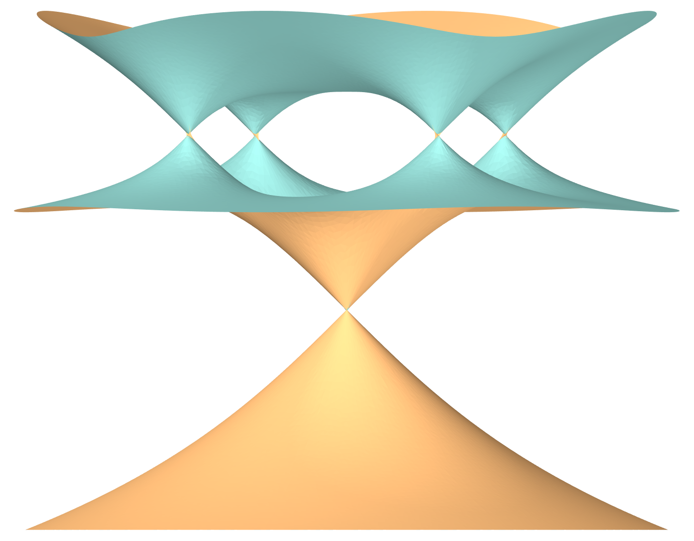
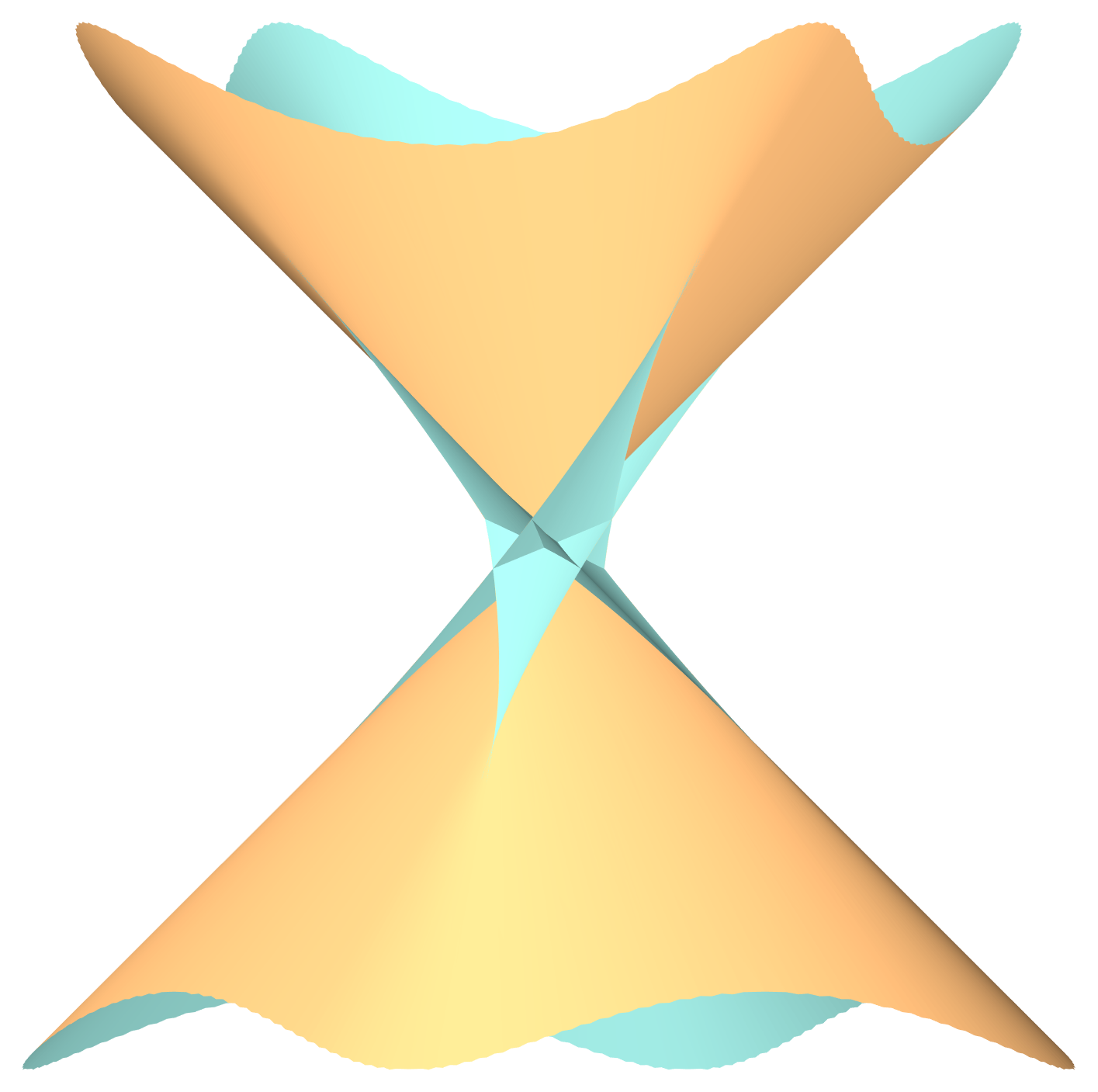
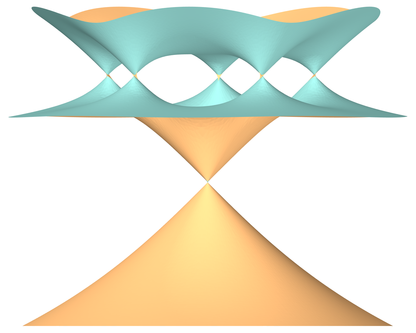
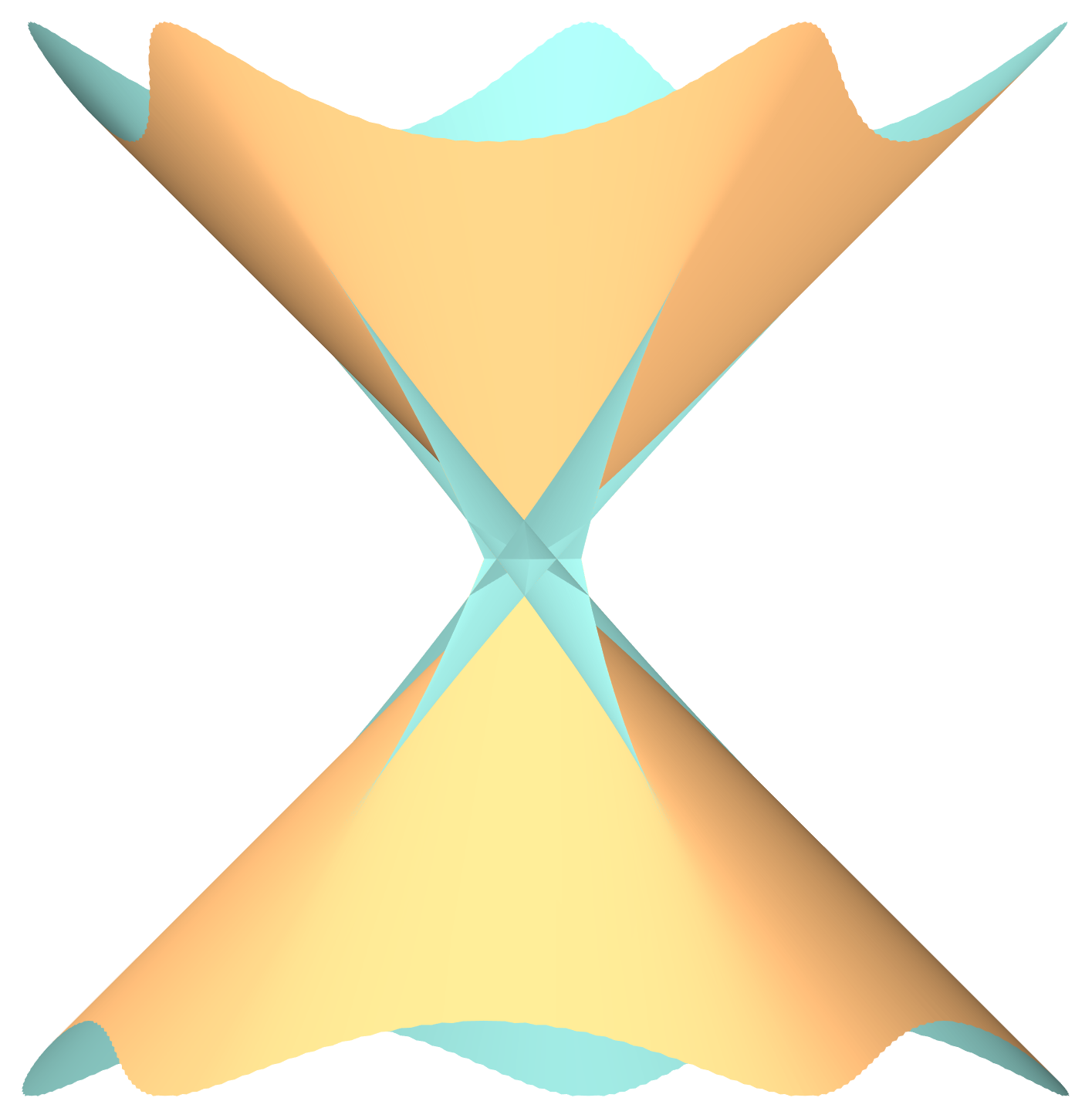
Figure 2. CHM sufaces with $m=4$ (top) and $m=5$ (bottom). On the right-hand side are the zoom-ins of the center neck, showing details of the cuspidal edges and swallowtails. To make this picture, we use the node-opening construction as in [traizet2008t], which is different but equivalent to the construction in the current paper, and better suited for numerical computations [traizet2008n].

4. Sketched construction

4.1. The Weierstrass data

We construct maxfaces using a Weierstrass–Enneper-like parameterization, namely

(4.1) $$M\ni z\mapsto\operatorname{Re}\int^{z}\Big{(}\frac{1}{2}(g^{-1}+g),\frac{i}{2}(g^{-1}-g),1\Big{)}dh\in{\mathbb{E}}^{3}_{1},$$

where $M$ is a Riemann surface, possibly with punctures corresponding to the ends, $g$ is a meromorphic function, and $dh$ a holomorphic $1$-form on $M$, subject to the following conditions:

Divisor condition:

Away from the punctures, we must have

$$(g)_{0}-(g)_{\infty}=(dh)_{0}$$

for the Weierstrass integrands to be holomorphic. The behavior at the punctures depend on the type of the ends.

Period condition:

For all closed curves $\gamma$ on $M$, we have

(4.2) $$\overline{\int_{\gamma}g^{-1}dh}+\int_{\gamma}gdh =0,$$

(4.3) $$\operatorname{Re}\int_{\gamma}dh =0.$$

So, closed curves in $M$ are mapped to closed curves on the surface. This guarantees that the immersion is well-defined.

Regularity condition:

$|g|$ is not identically $1$. In fact, the pullback metric on the Riemann surface $M$ is given by $ds^{2}=\frac{1}{4}\left(|g|^{-1}-|g|\right)^{2}|dh|^{2}$. In view of the divisor condition, the singularity set for maxfaces is then given by $\{p\in M:|g(p)|=1\}$. The regularity condition guarantees that the immersion is regular.

Remark 4.1.

For minimal surface, the horizontal period condition (4.2) would have a minus sign in the middle, and the pull-back metric would have a plus sign.

4.1.1. The Riemann Surface

We construct the Riemann surface by node-opening as follows:

To each of the $L$ horizontal (spacelike) planes is associated a copy of the complex plane ${\mathbb{C}}$, which can be seen as the Riemann sphere with punctures at $\infty$. The $L$ copies of ${\mathbb{C}}$, as well as their punctures, are then indexed by $l$, $1\leq l\leq L$. To each neck at level $l$, $1\leq l<L$ is associated a puncture $a_{l,k}\in{\mathbb{C}}_{l}$ and a puncture $b_{l,k}\in{\mathbb{C}}_{l+1}$, $1\leq k\leq n_{l}$.

Initially at $t=0$, we simply identify $a_{l,k}$ with $b_{l,k}$ for all $1\leq l<L$ and $1\leq k\leq n_{l}$ to obtain a noded Riemann surface $\Sigma_{0}$. As $t$ increases, fix local coordinates $v_{l,k}$ in the neighborhood of $a_{l,k}$, and local coordinates $w_{l,k}$ in the neighborhood of $b_{l,k}$; a concrete choice will be made soon later. We may fix an $\varepsilon$ sufficiently small and independent of $l$ and $k$ so that the disks $|v_{l,k}|<2\varepsilon$ and $|w_{l,k}|<2\varepsilon$ are all disjoint. For $t<\varepsilon$, we may remove the disks $|v_{l,k}|<t^{2}/\varepsilon$ and $|w_{l,k}|<t^{2}/\varepsilon$, and identify the annuli

$$t^{2}/\varepsilon<|v_{l,k}|<\varepsilon\qquad t^{2}/\varepsilon<|w_{l,k}|<\varepsilon$$

by

$$v_{l,k}w_{l,k}=t^{2}.$$

The resulting Riemann surface is denoted by $\Sigma_{t}$.

4.1.2. Gauss map and local coordinates

We define on ${\mathbb{C}}_{l}$ the meromorphic function

$$g_{l}:=\sum_{k=1}^{n_{l}}\frac{\alpha_{l,k}}{z-a_{l,k}}+\sum_{k=1}^{n_{l-1}}\frac{\beta_{l-1,k}}{z-b_{l-1,k}}.$$

Then the Gauss map $g$ is defined on $\Sigma_{t}$ as

$$g(z)=\begin{cases}tg_{l}(z)&\text{if }z\in{\mathbb{C}}_{l}\text{ and $l$ is odd,}\\ 1/(tg_{l}(z))&\text{if }z\in{\mathbb{C}}_{l}\text{ and $l$ is even.}\end{cases}$$

As $t\to 0$, the Gauss map converges to that of catenoids around the necks. Note that $1/g_{l}$ provides local coordinates $v_{l,k}$ around $a_{l,k}$ and $w_{l-1,k}$ around $b_{l-1,k}$. From now on, we adopt these local coordinates for the construction of $\Sigma_{t}$.

4.1.3. The height differential

Recall the period conditions $\operatorname{Re}\int_{\gamma}dh=0$ for every closed cycles $\gamma$ of $\Sigma_{t}$. Define

$$\Omega_{l}:=\{z\in{\mathbb{C}}_{l}:|v_{l,i}|<\varepsilon\quad\forall 1\leq i\leq n_{l}\quad\text{and}\quad|w_{l-1,j}|<\varepsilon\quad\forall 1\leq j\leq n_{l-1}\},$$

where $\varepsilon$ was previously fixed for the construction of $\Sigma_{t}$. Let $\gamma_{l,k}$ be small clockwise circles in $\Omega_{l}$ around $a_{l,k}$; they are homologous to counterclockwise circles in $\Omega_{l+1}$ around $b_{l}$. We close the vertical periods by requiring that $\int_{\gamma_{l,k}}dh=2\pi ir_{l,k}$ for real numbers $r_{l,k}$. Moreover, as we expect catenoid ends at $\infty_{l}$, we require that the height differential $dh$ has simple poles of residues $-R_{l}\in{\mathbb{R}}$ at $\infty_{l}$, $1\leq l\leq L$. By the Residue Theorem, it is necessary that $\sum R_{l}=0$ and

$$\sum_{k=1}^{n_{l}}r_{l,k}-\sum_{k=1}^{n_{l-1}}r_{l-1,k}=-R_{l}.$$

So, it suffices to prescribe the residue $-R_{k}$ and the periods around $\gamma_{l,k}$ for $1<k\leq n_{l}$.

By [traizet2002e], these requirements uniquely determine the height differential $dh$. Moreover, as $t\to 0$, $dh$ converges uniformly on a compact set of $\Omega_{l}$ to the form

(4.4) $$\sum_{k=1}^{n_{l}}\frac{-r_{l,k}dz}{z-a_{l,k}}+\sum_{i=1}^{n_{l-1}}\frac{r_{l-1,k}dz}{z-b_{l-1,k}}$$

We want catenoid or planar ends at the punctures $\infty_{l}$. This translates to the following divisor condition at $\infty_{l}$: Whenever $g$ has a simple zero or pole there, $dh$ must have a simple zero; this corresponds to the catenoid ends. On the other hand, whenever $g$ has a zero or pole of multiplicity $m>1$ at $\infty_{l}$, $dh$ must have a zero or multiplicity $m-2$; this corresponds to the planar ends. Because $dz$ has a pole of order $2$ at the punctures $\infty$, our divisor condition can be formulated as

(4.5) $$(g)_{0}-(g)_{\infty}=(dh/dz)_{0}.$$

4.2. Using the Implicit Function Theorem

We want to find parameters $X=(t,a,b,\alpha,\beta,r,R)$ that solve the divisor conditions, period conditions, and regularity conditions. All parameters vary in a neighborhood of their initial values at $t=0$, denoted by $X^{\circ}$. Given a balanced configuration $(l,p,c)$, we will see that

$$t^{\circ}=0,\quad R_{l}^{\circ}=Q_{l},$$

$$\forall 1\leq k\leq n_{l},r_{l,k}^{\circ}=-\alpha_{l,k}^{\circ}=\beta_{l,k}^{\circ}=c_{l}$$

$$\forall 1\leq k\leq n_{l},a_{l,k}^{\circ}=\overline{b_{l,k}^{\circ}}=\begin{cases}\overline{p_{l,k}},&l\text{ odd}\\ p_{l,k},&l\text{ even}.\end{cases}$$

The argument in [traizet2002e] applies, word by word, to prove the following

Proposition 4.2 (Divisor condition).

For $(t,a,b,r,R)$ in a neighborhood of their initial values, there exist unique values for $\alpha$ and $\beta$, depending analytically on $(t,a,b,r,R)$, such that the divisor conditions are satisfied. Moreover, at $t=0$, we have $-\alpha_{l,k}=\beta_{l,k}=r_{l,k}$.

For $1\leq l<L$, $1<k\leq n_{l}$, let $\Gamma_{l,k}$ be a closed curve that starts in $\Omega_{l}$, travels first through the neck $(l,1)$ to $\Omega_{l+1}$, then through the neck $(l,k)$ back to $\Omega_{l}$, and finally close itself. See [traizet2002e] for formal definitions of these curves. For $1\leq l<L$ and $1<k\leq n_{l}$, the curves $\Gamma_{l,k}$ and the previously defined $\gamma_{l,k}$ form a homology basis. So, we only need to close periods on these curves to solve the period conditions.

Recall that the vertical periods are already closed when defining the height differential $dh$. In the following proposition, we need to switch to the parameter $\tau$ given by $t=\exp(-1/\tau^{2})$. Again, The argument in [traizet2002e] applies word by word. The key point is that $-\tau^{-2}\int_{\Gamma_{l,k}}dh$ extends to a smooth function at $\tau=0$ with the value $2(r_{l,k}-r_{l,1})$.

Proposition 4.3 (Vertical periods).

Assume that $(\alpha,\beta)$ are given by the previous proposition. For $(\tau,a,b,R)$ in a neighborhood of their initial values, there exists unique values for $r$, depending smoothly on $(\tau,a,b,R)$, such that the vertical period condition (4.3) are satisfied over the curves $\Gamma_{l,k}$, $1\leq l<L$ and $1<k\leq n_{l}$. Moreover, at $\tau=0$, we have $r_{l,k}=c_{l}$ for all $1\leq k\leq n_{l}$ and $1\leq l<L$, where $c_{l}$ are defined from $R_{l}$ by $c_{0}=c_{L}=0$ and $c_{l-1}n_{l-1}-c_{l}n_{l}=R_{l}$.

The proof for the following step differs from minimal surfaces [traizet2002e] only by a few signs. This slight difference comes from the sign change in the horizontal period condition (4.2). We will give a sketch to point out the difference.

Proposition 4.4 (Horizontal periods).

Given a balanced and rigid configuration $(p,Q)$ such that the map $Q\to W$ has rank $1$. Assume that $(\alpha,\beta,r)$ are given by previous propositions. For $\tau$ in a neighborhood of $0$, there exists unique values for $a$, $b$, and $R$, depending smoothly on $\tau$, such that $\sum R_{l}=0$ and the horizontal period condition (4.2) are satisfied over the curves $\Gamma_{l,k}$ and $\gamma_{l,k}$, $1\leq l<L$ and $1<k\leq n_{l}$. Moreover, at $\tau=0$, up to a translation in ${\mathbb{C}}_{l}$, we have $a_{l,k}=\overline{b_{l,k}}=\overline{p_{l,k}}$ if $l$ is odd, $=p_{l,k}$ if $l$ is even, and $R_{l}=Q_{l}$.

Sketched proof.

Define the horizontal period along a curve $c$ as

$$P(c)=\overline{\int_{c}g^{-1}dh}+\int_{c}gdh.$$

Then $tP(\Gamma_{l,k})$ is extends to a smooth function at $\tau=0$ with the values

$$\begin{cases}b_{l,k}-b_{l,1}+\overline{a_{l,1}}-\overline{a_{l,k}},&l\text{ odd};\\ \overline{b_{l,k}}-\overline{b_{l,1}}+a_{l,1}-a_{l,k},&l\text{ even}.\end{cases}$$

If we normalize $b$ by fixing $b_{l,1}=\overline{a_{l,1}}$, then $tP(\Gamma_{l,k})$ vanish at $\tau=0$ if $b_{l,k}=\overline{a_{l,k}}$. As the partial differential of $tP(\Gamma_{l,k})$ with respect to $b$ is a linear isomorphism, the parameters $b$ are found by the Implicit Function Theorem.

Using these values of $b$, $t^{-1}P(\gamma_{l,k})$ extends to a smooth function at $\tau=0$ with the values

$$\begin{dcases}-4\pi i\Bigg{(}\sum_{1\leq j\neq k\leq n_{l}}\frac{2c_{l}^{2}}{a_{l,k}-a_{l,j}}-\sum_{j=1}^{n_{l+1}}\frac{c_{l}c_{l+1}}{a_{l,k}-\overline{a_{l+1,j}}}-\sum_{j=1}^{n_{l-1}}\frac{c_{l}c_{l-1}}{a_{l,k}-\overline{a_{l-1,j}}}\Bigg{)},&l\text{ odd},\\ 4\pi i\Bigg{(}\sum_{1\leq j\neq k\leq n_{l}}\frac{2c_{l}^{2}}{\overline{a_{l,k}}-\overline{a_{l,j}}}-\sum_{j=1}^{n_{l+1}}\frac{c_{l}c_{l+1}}{\overline{a_{l,k}}-a_{l+1,j}}-\sum_{j=1}^{n_{l-1}}\frac{c_{l}c_{l-1}}{\overline{a_{l,k}}-a_{l-1,j}}\Bigg{)},&l\text{ even}.\end{dcases}$$

They vanish at $t=0$ if $a_{l,k}=\overline{p_{l,k}}$ where $p$ is from a balanced configuration. Since the configuration is rigid, we may re-normalize $a$ by fixing two of the $a$ parameters, then use the Implicit Function Theorem to find the remaining $N-2$ $a$ parameters, depending smoothly on $t$ that solves $t^{-1}P(\gamma_{l,k})=0$ for all but two necks.

It remains to solve $P(\gamma_{l,k})=0$ for the remaining two necks. It is necessary that $n_{l_{0}}>1$ for some $l_{0}$; otherwise, the configuration would not be balanced unless $N=1$. So we may assume that the remaining necks are labeled by $(l_{0},1)$ and $(l_{0},k_{0})$, $1<k_{0}\leq n_{l_{0}}$. The relation that $P(\gamma_{l_{0},1})+P(\gamma_{l_{0},k_{0}})=0$ follows from the Residue Theorem. The Riemann Bilinear Relation shows that

$$\operatorname{Re}\Big{(}P(\gamma_{l_{0},k_{0}})\int_{\Gamma_{l_{0},k_{0}}}g^{-1}dh\Big{)}=0.$$

And finally, we study the function

$$G=\operatorname{Im}\Big{(}\sum_{l=1}^{L}\sum_{k=1}^{n_{k}}(-1)^{k}\overline{p_{l,k}}t^{-1}P(\gamma_{l,k})\Big{)}.$$

It extends to a smooth function at $\tau=0$ with the values of $4\pi W$, which vanishes because the configuration is balanced. Since the partial differential of $W$ with respect to $R$ is surjective at $t=0$, we may use the Implicit Function Theorem to find $R$, depending smoothly on $\tau$ in a neighborhood of $0$, such that $\sum R_{l}=0$ and $G(\tau,R)=0$. These conclude the proof that $P(\gamma_{l_{0},1})=P(\gamma_{l_{0},k_{0}})=0$. ∎

We have constructed a family of maximal maps.

$$(X_{1},X_{2},X_{3}):\Sigma_{t}\to{\mathbb{E}}^{3}_{1}.$$

Let $0_{k}$ be the origin point of ${\mathbb{C}}_{k}$. With a translation if necessary, we may assume that $0_{k}\in\Omega_{k}$. With similar computations as in [traizet2002e], one verifies that

• The necks converge to Lorentzian catenoids and, after a scaling by $t$, the limit positions of the necks are $p_{l,k}$.

• The image of $\Omega_{k}$ is a space-like graph over the horizontal plane and this image stays within a bounded distance from $X_{3}(0_{k})+R_{k}\log(1+t|x_{1}+ix_{2}|)$.

• $X_{3}(0_{k})-X_{3}(0_{k+1})=O(-\log t)$. So, if $Q_{k}<Q_{k+1}$, then for sufficiently small $t$, we have $R_{k}\leq R_{k+1}$ and the image of $\Omega_{k}$ is above the image of $\Omega_{k+1}$.

The singular set, given by $|v_{l,k}|=t$ and $|w_{l,k}|=t$, is compact in $\Sigma_{t}$, and is not included in $\Omega_{k}$. We then have proved that the constructed maximal maps are in fact maxface. Moreover these are embedded in a wider sense for sufficiently small $t$ if $Q_{1}<Q_{2}<\cdots<Q_{L}$.

5. Singularities

Recall that the singular set is given by $|g|=1$. From our definition of the Gauss map, the singularity set of the maxface $X_{t}$ is given by the union of

$$\mathcal{S}_{l,k}=\{z\in{\mathbb{C}}_{l}:|v_{l,k}|=t\}=\{z\in{\mathbb{C}}_{l+1}:|w_{l,k}|=t\}$$

with $1\leq l\leq N-1,1\leq k\leq n_{l}$. In this section, we aim to analyze the nature of these singularities.

For this purpose, we will focus on singularities around a specific neck of interest, labeled by $(l,k)$. Without loss of generality, we may assume that $l$ is odd. So the Gauss map $g_{t}=t/v_{l,k}=w_{l,k}/t$ in the local coordinates. To ease the text, we will omit the subscript $(l,k)$ unless necessary. So we study the connected component $\mathcal{S}$ of the singular set given by $|v|=|w|=t$.

5.1. The governing function

We need to study the function

(5.1) $${\mathcal{A}}(t,\theta)=-\frac{g_{t}(dh_{t}/dv)}{dg_{t}/dv}\Big{|}_{v=e^{i\theta}}=te^{i\theta}f_{t}(te^{i\theta}),$$

where $f_{t}:=dh_{t}/dv$.

Let $p$ be a singular point with $v(p)=te^{i\theta}$. On the one hand, it was proved in [umehara2006] that the parameterization (4.1) is a front (that is, the projection of a Legendrian immersion into the unit cotangent bundle of ${\mathbb{R}}^{3}$) on a neighborhood $U$ of a singular point $p$ and $p$ is a nondegenerate singular point (meaning $d\lambda=0$ where $\lambda^{2}$ is the determinant of the Euclidean metric tensor) if and only if $\operatorname{Re}(1/{\mathcal{A}}(t,\theta))\neq 0$. If this is the case, the singular set $\mathcal{S}$ is a smooth singular curve in $U$ that passes through $p$. In our case, the singular curve $\gamma_{t}(\theta)$ is actually given by $v(\gamma_{t}(\theta))=te^{i\theta}$, $0\leq\theta<2\pi$.

On the other hand, it was shown in [umehara2006] that

$$\det(\dot{\gamma}_{t}(\theta),\eta_{t}(\theta))=\operatorname{Im}(1/{\mathcal{A}}(t,\theta)),$$

where $\dot{\gamma}_{t}$ is the singular direction and $\eta_{t}\in\operatorname{Ker}(dX_{t})$ is the null direction. So $\operatorname{Im}(1/{\mathcal{A}})$ measures the collinearity between the $\dot{\gamma}$ and $\eta$.

In particular, $p=te^{i\theta}$ is a cuspidal singularity whenever

(5.2) $$\operatorname{Re}{\mathcal{A}}(t,\theta)\neq 0\quad\text{and}\quad\operatorname{Im}{\mathcal{A}}(t,\theta)\neq 0,$$

and $p$ is a swallowtail singularity whenever

(5.3) $$\operatorname{Re}{\mathcal{A}}\neq 0,\quad\operatorname{Im}{\mathcal{A}}=0,\quad\text{and}\quad\frac{\partial}{\partial\theta}\operatorname{Im}{\mathcal{A}}\neq 0.$$

In fact, the cuspidals are $A_{2}$ singularities, the swallowtails are $A_{3}$ singularities and the butterflies are $A_{4}$ singularities. More generally, one may define [honda2021] that $p$ is a generalized $A_{k+2}$ singularity if

(5.4) $$\operatorname{Re}{\mathcal{A}}\neq 0,\quad\operatorname{Im}{\mathcal{A}}=\frac{\partial}{\partial\theta}\operatorname{Im}{\mathcal{A}}=\cdots\frac{\partial^{k-1}}{\partial\theta^{k-1}}\operatorname{Im}{\mathcal{A}}=0,\quad\frac{\partial^{k}}{\partial\theta^{k}}\operatorname{Im}{\mathcal{A}}\neq 0.$$

It was proved [izumiya2012, kokubu2005] that generalized $A_{k}$ singularities with $k=2,3,4$ are indeed $A_{k}$ singularities, but this is not known for $k\geq 5$.

5.2. Nondegeneracy

Recall that $dh_{t}$ extend real analytically to $t=0$ with the form given by (4.4), with simple poles of residue $-r_{l,k}$ at the nodes at $a_{l,k}$. Because $-r_{l,k}\to-c_{l}$ as $t\to 0$, we have ${\mathcal{A}}(t,\theta)\to-c_{l}\neq 0$ no matter the value of $\theta$. This implies that $A(t,\theta)$ extends real analytically to $t=0$ with a non-zero finite value independent of $\theta$. So $\operatorname{Re}(1/{\mathcal{A}}(t,\theta))$ extends real analytically to $t=0$ with a non-zero value independent of $\theta$. By continuity, we have $\operatorname{Re}(1/{\mathcal{A}})\neq 0$ for sufficiently small $t$.

This proves that, for sufficiently small non-zero $t$, the Weierstrass parameterization defines a front in a neighborhood of the singular points, and the singular points are all nondegenerate. Note that, for sufficiently small $t$, the singular set is a circle of radius $t$ in the local coordinate $v$, which obviously defines a smooth curve. So, the nondegeneracy of the singular points is expected.

5.3. Non-cuspidal singularities

The node opening could also be implemented by an identification $vw=s$ where $s$ is a complex parameter. It was proved in [traizet2002e] that the height differential $dh$ depends holomorphically on $s$ and $v$, and extends holomorphically to $s=0$. In our case, we have $vf_{t}$ extends holomorphically to $(s,v)=(0,0)$ with the value $-c_{l}$. So ${\mathcal{A}}(t,\theta)$ depends real analytically on $t$ and $\theta$, and extends real analytically to $t=0$ with the value $-c_{l}$ independent of the value of $\theta$.

The singularity is cuspidal when $\operatorname{Im}{\mathcal{A}}\neq 0$. So, the set of non-cuspidal singularities around a neck, given as the zero locus $\operatorname{Im}{\mathcal{A}}=0$, is a real analytic variety.

If the zero locus has a non-zero measure, then $\operatorname{Im}{\mathcal{A}}\equiv 0$, and the singular curve is mapped to a single point, so we have a cone singularity no matter $t$ and $\theta$ [fujimori2009].

Otherwise, by Lojasiewicz’s theorem, the non-cuspidal singular set can be stratified into a disjoint union of real analytic curves ($1$-strata) and discrete points ($0$-strata). In particular, $t=0$ is a trivial solution of $\operatorname{Im}{\mathcal{A}}=0$, and there is no $0$-strata for $t\neq 0$ sufficiently small. In other words, in a neighborhood of $t=0$, the set of non-cuspidal singularities is given by disjoint curves. See Figure 3.

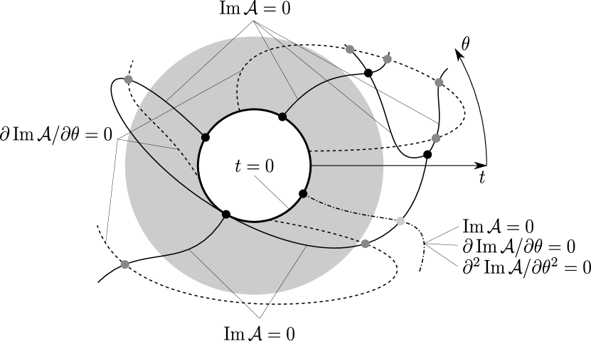
Figure 3. Sketch of a typical structure of non-cuspidal singularities. The circle in the middle is the trivial locus with $t=0$. Solid curves are solutions to $\operatorname{Im}{\mathcal{A}}=0$. Dashed curves are solutions to $\partial\operatorname{Im}{\mathcal{A}}/\partial\theta=0$. Dots indicate the $0$-strata. The grey dots at the intersection of solid and dashed curves are then at least butterfly singularities. The dot-dashed curve indicates a possible curve that solves $\operatorname{Im}{\mathcal{A}}=\partial\operatorname{Im}{\mathcal{A}}/\partial\theta=\partial^{2}\operatorname{Im}{\mathcal{A}}/\partial\theta^{2}=0$. Singularities on this curve are then at least generalized $A_{5}$ singularities. The grey area indicates a neighborhood of the trivial locus that includes no $0$-strata of the variety. The variety appears as disjoint curves within this neighborhood.

More generally, the set of generalized $A_{k}$-singularities, $k>0$, is a real-analytic variety given by the zero locus

$$\mathcal{Z}_{k}=\{(t,\theta):\operatorname{Im}{\mathcal{A}}=\frac{\partial}{\partial\theta}\operatorname{Im}{\mathcal{A}}=\cdots\frac{\partial^{k-1}}{\partial\theta^{k-1}}\operatorname{Im}{\mathcal{A}}=0\}.$$

Again, by Lojasiewicz’s theorem, the locus can be stratified into curves and discrete points and contains the trivial solution $t=0$. In particular, if the singularities are of type $A_{k}$ along a segment of a curve in $\mathcal{Z}_{k}$, then the type will remain along this curve until hitting a $0$-stratum of $\mathcal{Z}_{k+1}$. See Figure 3.

We have proved the following

Theorem 5.1.

For $t\neq 0$ sufficiently small, if the height differential $dh_{t}$ is not identically $0$ (as a function of $t$ and $\theta$), then the non-cuspidal singularities around a neck are described by a disjoint union of finitely many curves in the $(t,\theta)$-plane, each given by a real-analytic function $\theta=\theta(t)$. Moreover, along each of these curves, the type of singularities is invariant for $t\neq 0$ sufficiently small.

5.4. Swallowtails

We have seen that, generically, a non-cuspidal singularity is a swallowtail. In this part, for sufficiently small non-zero $t$, we want to identify swallowtails using the Implicit Function Theorem. The strategy is the following:

We first remove the trivial solutions $t=0$ by considering the function

(5.5) $$\widetilde{\mathcal{A}}(t,\theta):=\operatorname{Im}{\mathcal{A}}(t,\theta)/t^{m},$$

which should extend to $t=0$ with the values $\widetilde{\mathcal{A}}(0,\theta)$ that is not identically $0$. Of course, this is only possible if $\operatorname{Im}{\mathcal{A}}(t,\theta)$ itself is not identically $0$. That is if the singularity is not cone-like. Then $\widetilde{\mathcal{A}}(0,\theta)$ could only have finitely many zeros. At a simple zero $\theta_{0}$, we may apply the Implicit Function Theorem on $\widetilde{\mathcal{A}}$. More specifically, if

$$\widetilde{\mathcal{A}}(0,\theta_{0})=0,\qquad\frac{\partial}{\partial\theta}\widetilde{\mathcal{A}}(0,\theta_{0})\neq 0$$

for some $\theta_{0}$, then for sufficiently small $t$, there exists a unique value for $\theta$ as a function of $t$, such that $\widetilde{\mathcal{A}}(t,\theta(t))=0$ and $\theta(t)$ extends to $t=0$ with the value $\theta(0)=\theta_{0}$. Moreover, $\frac{\partial}{\partial\theta}\widetilde{\mathcal{A}}(t,\theta(t))\neq 0$ for sufficiently small non-zero $t$. In other words, the singularities are swallowtails along the curve $\theta=\theta(t)$. Unfortunately, if $\theta_{0}$ is a multiple zero of $\widetilde{\mathcal{A}}$, we are not able to draw concrete conclusions on the numbers and types of the singularities in the neighborhood $(0,\theta_{0})$.

Now, the problem reduces to finding $\widetilde{\mathcal{A}}$. If $\frac{\partial^{k}}{\partial t^{k}}\operatorname{Im}{\mathcal{A}}(0,\theta)\equiv 0$ for all $0\leq k<m$, then $\frac{\partial^{m}}{\partial t^{m}}\operatorname{Im}{\mathcal{A}}(t,\theta)$ extends to $t=0$ with the value

$$\frac{\partial^{m}}{\partial t^{m}}\operatorname{Im}{\mathcal{A}}(0,\theta)=m!\lim_{t\to 0}\frac{\operatorname{Im}{\mathcal{A}}(t,\theta)}{t^{m}}.$$

Therefore, let $m$ be the smallest integer $k$ such that $\frac{\partial^{k}}{\partial t^{k}}{\mathcal{A}}(0,\theta)\not\equiv 0$, then

$$\widetilde{\mathcal{A}}(t,\theta)=\frac{\operatorname{Im}{\mathcal{A}}(t,\theta)}{t^{m}}=\frac{1}{m!}\frac{\partial^{m}}{\partial t^{m}}\operatorname{Im}{\mathcal{A}}(t,\theta)+o(1)$$

for $t$ in a neighborhood of $0$, and extends to $t=0$ with the value $\frac{1}{m!}\frac{\partial^{m}}{\partial t^{m}}\operatorname{Im}{\mathcal{A}}(0,\theta)$.

In the Appendix, we compute that the partial derivatives

(5.6) $$\frac{1}{m!}\frac{\partial^{m}{\mathcal{A}}}{\partial t^{m}}(0,\theta)=\lim_{t\to 0}\sum_{0\leq n\leq m-1}\frac{1}{(m-n-1)!}\frac{\partial^{m-n-1}}{\partial t^{m-n-1}}(a_{n}e^{i(n+1)\theta}-b_{n}e^{-i(n+1)\theta}).$$

where

$$a_{n}=\frac{1}{2\pi i}\int_{|v|=\varepsilon}\frac{dh_{t}}{v^{n+1}},\quad b_{n}=\frac{1}{2\pi i}\int_{|w|=\varepsilon}\frac{dh_{t}}{w^{n+1}}$$

are coefficients in the Laurent expansions of $dh_{t}$ in the ${\mathbb{C}}_{l}$ and ${\mathbb{C}}_{l+1}$, respectively. Recall that, at $t=0$, $dh_{t}/dv=g_{l}=1/v$ on ${\mathbb{C}}_{l}$, so

$$a_{n}=\operatorname{Res}_{0}g_{l}^{n+2},\quad b_{n}=\operatorname{Res}_{0}g_{l+1}^{n+2}.$$

In particular,

$$\frac{\partial{\mathcal{A}}}{\partial t}(0,\theta)=\lim_{t\to 0}(a_{0}e^{i\theta}-b_{0}e^{-i\theta}).$$

Note that, at $t=0$, we have

$$\overline{a_{0}} =\sum_{1\leq j\neq k\leq n_{l}}\frac{c_{l}}{p_{l,k}-p_{l,j}}-\sum_{1\leq j\leq n_{l-1}}\frac{c_{l-1}}{p_{l,k}-p_{l-1,j}},$$

$$b_{0} =\sum_{1\leq j\neq k\leq n_{l}}\frac{c_{l}}{p_{l,k}-p_{l,j}}-\sum_{1\leq j\leq n_{l+1}}\frac{c_{l+1}}{p_{l,k}-p_{l+1,j}},$$

so $\overline{a_{0}}+b_{0}=F_{l,k}/c_{l}$, which vanishes by the balance condition. Therefore, $\frac{\partial}{\partial t}{\mathcal{A}}(0,\theta)=2\operatorname{Re}(a_{0}e^{i\theta})$ is real, hence $\frac{\partial}{\partial t}\operatorname{Im}{\mathcal{A}}(0,\theta)=0$. This implies that $m>1$ in (5.5).

Then, we must look at the next derivative, namely

$$\frac{1}{2}\frac{\partial^{2}{\mathcal{A}}}{\partial t^{2}}(0,\theta)=\lim_{t\to 0}(a_{1}e^{2i\theta}-b_{1}e^{-2i\theta})+\lim_{t\to 0}\frac{\partial}{\partial t}(a_{0}e^{i\theta}-b_{0}e^{-i\theta}).$$

Note that the node opening process remains the same if we replace $t$ by $-t$, so $dh_{t}$, as well as its Laurent coefficients, are even in $t$. So, the second limit vanishes in the formula above. The imaginary part of the first limit equals $R^{(1)}(\theta)$ as defined in Section 2. If it does not vanish, then $m=2$ in (5.5), and $\widetilde{\mathcal{A}}(0,\theta)$ is given by a shifted sine function of period $\pi$. We then conclude that

Proposition 5.2.

If $R^{(1)}(\theta)\not\equiv 0$ at $t=0$, there are four non-cuspidal singularities around the neck for sufficiently small non-zero $t$, they are all swallowtails and, as $t\to 0$, the differences between the angles $\theta$ of neighboring swallowtails tend to $\pi/2$. In other words, these swallowtails tend to be evenly distributed as $t\to 0$.

Otherwise, if $R^{(1)}(\theta)\equiv 0$ at $t=0$, we must look at higher order derivatives of ${\mathcal{A}}$ and continue the analysis. But things become significantly more complicated, mainly because we don’t have control over even-order derivatives of the $a_{n}$ and $b_{n}$.

5.5. Symmetries

We can say more about the singularities if symmetries are imposed to the maxfaces.

Proposition 5.3.

Assume that the configuration has a rotational symmetry of order $r>1$ and the neck of interest is at the rotation center. If $R^{(r-1)}(\theta)\not\equiv 0$, then there are $2r$ non-cuspidal singularities around the neck for sufficiently small non-zero $t$, they are all swallowtails and, as $t\to 0$, the differences between the angles $\theta$ between neighboring swallowtails tend to $\pi/r$. In other words, these swallowtails tend to be evenly distributed as $t\to 0$.

Proof.

Under the assumed symmetry, $vf=vdh_{t}/dv$ is a function of $v^{r}$, hence $a_{0}=b_{1}=\cdots=a_{r-2}=b_{r-2}=0$ for all $t$. then $m\geq r-1$ in (5.5) and the equality holds if $R^{(r-1)}(\theta)\not\equiv 0$ at $t=0$. In the case of equality, $\widetilde{\mathcal{A}}(0,\theta)$ is given by a shifted sine function of period $2\pi/r$. ∎

Proposition 5.4.

Assume that the configuration has a vertical reflection plane that cuts through the neck of interest. Then, the singularity around the neck that is fixed by the reflection is non-cuspidal.

Proof.

We may further assume that the singular point $p$ fixed by the reflection is given by $v(p)=t$. Then, the height differential is real on the real line under the local coordinate $v$. So, all the Laurent coefficients are real no matter the value of $t$. In particular, $\operatorname{Im}{\mathcal{A}}(t,0)=0$, so $p$ is a non-cuspidal singularity. ∎

Remark 5.5.

For sufficiently small non-zero $t$, a singularity around the neck that is fixed by a vertical reflection could be a generalized $A_{k}$ singularity only for odd $k$.

Remark 5.6.

By the two propositions above, if a configuration has a dihedral symmetry of order $2r$ and the neck of interest is at the symmetry center, then there are $2r$ swallowtails around the neck with the same dihedral symmetry.

Proposition 5.7.

Assume that the configuration of necks has a horizontal reflection plane that cuts through the neck of interest. Then, the singular curve around the neck is mapped to a conelike singularity.

Proof.

Under the assumed symmetry, the singular curve is pointwise fixed by an antiholomorphic involution $\iota:v\mapsto w=t^{2}/v$ of the Riemann surface $\Sigma_{t}$, and $\iota^{*}(dh)=-\overline{dh}$. In other words, we have $a_{n}+\overline{b_{n}}=0$ for all $n\in{\mathbb{Z}}$ no matter the value of $t$. As a consequence, the partial derivatives of ${\mathcal{A}}$ over $t$ are all real, so $\operatorname{Im}{\mathcal{A}}\equiv 0$. ∎

Appendix A Derivatives of ${\mathcal{A}}$

The height differential $dh_{t}$ for the maxface, as defined in Section 4.1.3, has the following Laurent expansion in the annulus $t^{2}/\varepsilon<v<\varepsilon$:

$$dh_{t}(v)=\sum_{n\in{\mathbb{Z}}}a_{n}(t)v^{n}dv,\quad dh_{t}(w)=\sum_{n\in{\mathbb{Z}}}b_{n}(t)w^{n}dw,$$

where

$$a_{n}=\frac{1}{2\pi i}\int_{|v|=\varepsilon}\frac{dh_{t}}{v^{n+1}},\quad b_{n}=\frac{1}{2\pi i}\int_{|w|=\varepsilon}\frac{dh_{t}}{w^{n+1}}.$$

Moreover, for each $n\in{\mathbb{Z}}$,

$$a_{n}=\frac{1}{2\pi i}\int_{|v|=\varepsilon}\frac{dh_{t}}{v^{n+1}}=\frac{-1}{2\pi i}\int_{|w|=\varepsilon}\frac{dh_{t}w^{n+1}}{t^{2n+2}}.$$

Therefore, we have

(A.1) $$\frac{\partial^{m}a_{n}}{\partial t^{m}}=\frac{-1}{2\pi i}\sum_{j=0}^{m}\int_{|w|=\varepsilon}w^{n+1}\binom{m}{j}\frac{\partial^{m-j}dh_{t}}{\partial t^{m-j}}(-2n-2)_{j}\frac{1}{t^{2n+2+j}}.$$

Here, $(a)_{j}=a(a-1)\cdots(a-j+1)$ (in particular $(a)_{0}=1)$ is the descending factorial. In particular, $(-2n-2)_{j}=0$ whenever $0\leq-2n-2<j$. Note that $dh_{t}$ and its derivatives are bounded on the circle $|w|=\varepsilon$.

We now prove Equation (5.6) for the partial derivatives of ${\mathcal{A}}$ over $t$. We repeat the formula below

$$\frac{1}{m!}\frac{\partial^{m}{\mathcal{A}}}{\partial t^{m}}(0,\theta)=\lim_{t\to 0}\sum_{0\leq n\leq m-1}\frac{1}{(m-n-1)!}\frac{\partial^{m-n-1}}{\partial t^{m-n-1}}(a_{n}e^{i(n+1)\theta}-b_{n}e^{-i(n+1)\theta}).$$

Proof.

Recall the expression (5.1) of ${\mathcal{A}}$

(A.2) $${\mathcal{A}}(t,\theta)=te^{i\theta}\frac{dh_{t}}{dv}(te^{i\theta})=\sum_{n\in{\mathbb{Z}}}a_{n}(t)t^{n+1}e^{i(n+1)\theta}=\sum_{n\in{\mathbb{Z}}}b_{n}(t)t^{n+1}e^{-i(n+1)\theta},$$

which can be expanded in terms of $t$ as follows

(A.3) $${\mathcal{A}}(t,\theta)=\sum_{m\geq 0}\frac{1}{m!}\frac{\partial^{m}{\mathcal{A}}}{\partial t^{m}}(0,\theta)t^{m}.$$

From (A.2), we have

$$\frac{1}{m!}\frac{\partial^{m}{\mathcal{A}}}{\partial t^{m}}(t,\theta) =\sum_{n\in{\mathbb{Z}}}\sum_{j=0}^{m}\binom{m}{j}\frac{(n+1)_{j}}{m!}\frac{\partial^{m-j}a_{n}}{\partial t^{m-j}}t^{n+1-j}e^{i(n+1)\theta}.$$

In the following, we will calculate the limits of the terms on the right-hand side as $t\to 0$. The computation is done case by case.

$n>m-1$:

Since derivative of $a_{n}$ is bounded, $\frac{\partial^{m-j}a_{n}}{\partial t^{m-j}}t^{n+1-j}\to 0$ as $t\to 0$ when $n>j-1$. In particular, this also holds when $n>m-1$. We conclude that, when $n>m-1$ and as $t\to 0$,

$$\sum_{j=0}^{m}\binom{m}{j}\frac{(n+1)_{j}}{m!}\frac{\partial^{m-j}a_{n}}{\partial t^{m-j}}t^{n+1-j}e^{i(n+1)\theta}\to 0.$$

$n=m-1$:

In this case, as $t\to 0$, we have

$$\sum_{j=0}^{m}\binom{m}{j}\frac{(m)_{j}}{m!}\frac{\partial^{m-j}a_{m-1}}{\partial t^{m-j}}t^{m-j}e^{im\theta}\to a_{m-1}e^{im\theta},$$

since derivatives of $a_{n}$ are bounded and, for $j<m$, $t^{m-j}\to 0.$

$0\leq n<m-1$:

In this case, as $t\to 0$, we have

$$\sum_{j=0}^{m}\binom{m}{j}\frac{(n+1)_{j}}{m!}\frac{\partial^{m-j}a_{n}}{\partial t^{m-j}}t^{n+1-j}e^{i(n+1)\theta}\to\frac{1}{(m-n-1)!}\frac{\partial^{m-n-1}a_{n}}{\partial t^{m-n-1}}e^{i(n+1)\theta},$$

since $j=n+1$ is the only non-zero term in the summation.

$n=-1$:

In this case, we have

$$\sum_{j=0}^{m}\binom{m}{j}\frac{(n+1)_{j}}{m!}\frac{\partial^{m-j}a_{n}}{\partial t^{m-j}}t^{n+1-j}e^{i(n+1)\theta}=0.$$

$-m\leq n\leq-2$:

In this case, we have

$$\frac{\partial^{m-j}a_{n}}{\partial t^{m-j}}t^{n+1-j} =\frac{-1}{2\pi i}\sum_{k=0}^{m-j}\int_{w=|\varepsilon|}w^{n+1}\binom{m-j}{k}\frac{\partial^{m-j-k}dh_{t}}{\partial t^{m-j-k}}(-2n-2)_{k}t^{-n-1-k-j}$$

$$\to\frac{-1}{2\pi i}\sum_{k=-n-1-j}^{m-j}\int_{w=|\varepsilon|}w^{n+1}\binom{m-j}{k}\frac{\partial^{m-j-k}dh_{t}}{\partial t^{m-j-k}}(-2n-2)_{k}t^{-n-1-k-j}.$$

By the identity

(A.4) $$\sum_{j=0}^{l}\binom{m}{j}\frac{(n+1)_{j}}{m!}\binom{m-j}{k}(-2n-2)_{k}\\ =\begin{dcases}\frac{1}{(m-n-1)!},&\text{ when }l=-n-1\\ 0,&\text{ when }l<-n-1\end{dcases},$$

where $l=j+k$ and $-m\leq n\leq-2$, we conclude that

$$\sum_{j=0}^{m}\binom{m}{j}\frac{(n+1)_{j}}{m!}\frac{\partial^{m-j}a_{n}}{\partial t^{m-j}}t^{n+1-j}\to\frac{-1}{(m+n+1)!}\frac{\partial^{m+n+1}}{\partial t^{m+n+1}}b_{-n-2}.$$

$n=-(m+1)$:

In this case,

$$\frac{\partial^{m-j}a_{-(m+1)}}{\partial t^{m-j}}t^{-m-j} =\frac{-1}{2\pi i}\sum_{k=0}^{m-j}\int_{|w|=\varepsilon}w^{-m}\binom{m-j}{k}\frac{\partial^{m-j-k}dh_{t}}{\partial t^{m-j-k}}(2m)_{k}\frac{1}{t^{-m+j+k}}$$

$$\to\frac{-1}{2\pi i}\int_{|w|=\epsilon}w^{-m}dh_{t}(2m)_{m-j}.$$

As $t\to 0$, we have

$$\sum_{j=0}^{m}\binom{m}{j}\frac{(-m)_{j}}{m!}\frac{\partial^{m-j}a_{-(m+1)}}{\partial t^{m-j}}t^{-m-j}e^{-im\theta}$$

$$\to \frac{-1}{2\pi i}\sum_{j=0}^{m}\binom{m}{j}\frac{(-m)_{j}}{m!}\int_{|w|=\epsilon}w^{-m}dh_{t}(2m)_{m-j}e^{-im\theta}$$

$$= \sum_{j=0}^{m}\binom{m}{j}\frac{(-m)_{j}}{m!}\frac{(2m)!}{(m+j)!}a_{-(m+1)}t^{-2m}e^{-im\theta}$$

$$= \sum_{j=0}^{m}\binom{m}{j}\frac{(-m)_{j}}{m!}\frac{(2m)!}{(m+j)!}(-1)b_{m-1}e^{-im\theta}.$$

By the identity

(A.5) $$\sum_{j=0}^{m}\binom{m}{j}\frac{(-m)_{j}(2m)_{m-j}}{m!}=1,\quad m>0,$$

we conclude that, as $t\to 0$,

$$\sum_{j=0}^{m}\binom{m}{j}\frac{(-m)_{j}}{m!}\frac{\partial^{m-j}a_{-m-1}}{\partial t^{m-j}}t^{-m-j}\to-b_{m-1}.$$

$n<-(m+1)$:

In this case, by (A.1)

$$\frac{\partial^{m-j}a_{n}}{\partial t^{m-j}}t^{n+1-j}=\frac{-1}{2\pi i}\sum_{k=0}^{m-j}\int_{|w|=\varepsilon}w^{n+1}\binom{m-j}{k}\frac{\partial^{m-j-k}dh_{t}}{\partial t^{m-j-k}}(-2n-2)_{k}\frac{1}{t^{n+1+j+k}}.$$

Since partial derivatives of $dh$ are bounded on $|w|=\epsilon$, $\frac{\partial^{m-j}a_{n}}{\partial t^{m-j}}t^{n+1-j}\to 0$ as $t\to 0$ when $n+1+j+k<0$. In particular, this also holds when $n<-(m+1)$. We conclude that, when $n<-(m+1)$ and as $t\to 0$,

$$\sum_{j=0}^{m}\binom{m}{j}\frac{(n+1)_{j}}{m!}\frac{\partial^{m-j}a_{n}}{\partial t^{m-j}}t^{n+1-j}e^{i(n+1)\theta}\to 0.$$

Gathering all these computations, we obtain

$$\frac{1}{m!}\frac{\partial^{m}A}{\partial t^{m}}(0,\theta) =\lim_{t\to 0}\Bigg{(}-\sum_{-m-1\leq n\leq-2}\frac{1}{(m+n+1)!}\frac{\partial^{m+n+1}}{\partial t^{m+n+1}}b_{-n-2}e^{i(n+1)\theta}$$

$$\quad\quad\quad\quad+\sum_{0\leq n\leq m-1}\frac{1}{(m-n-1)!}\frac{\partial^{m-n-1}a_{n}}{\partial t^{m-n-1}}e^{i(n+1)\theta}\Bigg{)}$$

$$=\lim_{t\to 0}\sum_{0\leq n\leq m-1}\frac{1}{(m-n-1)!}\frac{\partial^{m-n-1}}{\partial t^{m-n-1}}(a_{n}e^{i(n+1)\theta}-b_{n}e^{-i(n+1)\theta}).$$

∎

Finally, we prove the two combinatorial identities (A.4) and (A.5) used in the proof above.

Proof of (A.5).

$$\sum_{j=0}^{m}\binom{m}{j}\frac{(-m)_{j}(2m)_{m-j}}{m!} =\sum_{j=0}^{m}(-1)^{j}\frac{m!(m+j-1)!(2m)!}{m!(m-j)!j!(m-1)!(m+j)!}$$

$$=\sum_{j=0}^{m}(-1)^{j}\frac{m}{m+j}\binom{m+j}{j}\binom{2m}{m+j}$$

$$=\sum_{j=0}^{m}(-1)^{j}\frac{m}{m+j}\binom{m}{j}\binom{2m}{m}$$

$$=m\binom{2m}{m}\sum_{j=0}^{m}\frac{(-1)^{j}}{m+j}\binom{m}{j}=1,$$

where the last line follows from

$$\sum_{j=0}^{m}\frac{(-1)^{j}}{m+j}\binom{m}{j} =\sum_{j=0}^{m}(-1)^{j}\binom{m}{j}\int_{0}^{1}x^{m+j-1}dx$$

$$=\int_{0}^{1}x^{m-1}\sum_{j=0}^{m}\binom{m}{j}(-x)^{j}dx=\int_{0}^{1}x^{m-1}(1-x)^{m}dx$$

$$=\frac{\Gamma(m)\Gamma(1+m)}{\Gamma(1+2m)}=\frac{(m-1)!m!}{(2m)!}=\frac{1}{m\binom{2m}{m}}.$$

∎

Proof of (A.4).

For each $-n-1\leq l=j+k\leq m$,

$$\sum_{j=0}^{l}\binom{m}{j}\frac{(n+1)_{j}}{m!}\binom{m-j}{k}(-2n-2)_{k} =\sum_{j=0}^{l}\binom{m}{l}\binom{l}{j}\frac{(n+1)_{j}}{m!}(-2n-2)_{l-j}$$

$$=\binom{m}{l}\frac{l!}{m!}\sum_{j=0}^{l}\binom{l}{j}\frac{(n+1)_{j}(-2n-2)_{l-j}}{l!}$$

which, by similar argument as before, equals $\frac{1}{(m+n+1)!}$ when $l=-n-1$. Otherwise, if $l>-n-1$, it

$$=\binom{m}{l}\frac{l!}{m!}\sum_{j=0}^{l}(-1)^{j}\frac{l!(-n+j-2)!(-2n-2)!}{l!(l-j)!j!(-n-2)!(-2n-2-l+j)!}$$

$$=\binom{m}{l}\frac{l!}{m!}\sum_{j=0}^{l}(-1)^{j}\binom{-n+j-2}{j}\binom{-2n-2}{-2n-2-l+j}$$

$$=\binom{m}{l}\frac{l!}{m!}\sum_{j=0}^{l}(-1)^{j}\frac{(-n-2+j)_{l+n}}{(-n-2)_{l+n}}\binom{-2n-2-l+j}{j}\binom{-2n-2}{-2n-2-l+j}$$

$$=\binom{m}{l}\frac{l!}{m!}\sum_{j=0}^{l}(-1)^{j}\frac{(-n-2+j)_{l+n}}{(-n-2)_{l+n}}\binom{l}{j}\binom{-2n-2}{-2n-2-l}=0$$

because $(-n-2+j)_{l+n}$ is a polynomial of $j$ of degree $0\leq l+n<l$. ∎