Optimal Design of Climate Disclosure Policies: Transparency versus Externality

Abstract

Does a more transparent climate disclosure policy induce lower emissions? This paper analyzes the welfare consequences of transparency in corporate disclosure regulation in an environment in which regulatory disclosure constitutes the sole avenue for the verification of a firm’s emissions. On the one hand, a potential trade-off between disclosure transparency and externality suggests a non-monotonic relationship between them. On the other hand, increased transparency never makes the firm worse off. Consequently, mandating full disclosure is no different from maximizing the firm’s private benefit while disregarding the ensuing externality. When the regulator is symmetrically informed about the firm’s energy efficiency level, transparency beyond binary disclosure does not lead to welfare improvements. In the presence of information asymmetry, the welfare-maximizing disclosure takes a threshold form: all emissions above the threshold are pooled together, whereas all emissions below are fully disclosed.

Keywords: Sustainable finance, Carbon disclosure, Information design.

JEL classification: G18; M48; Q58.

1 Introduction

Recent years have witnessed an unprecedented surge in public awareness of climate impacts, and the financial sector is no exception. Investors have been showing a growing interest in scrutinizing the environmental impacts of the firms they consider for investment, calling for greater transparency in the disclosure of corporate carbon footprints. In response to this demand, the regulation of corporate climate disclosure has taken center stage on the agenda of the policymakers. From a welfare perspective, disclosing firms’ climate-related activities, such as their greenhouse gas emissions, serves to hold these firms accountable for their actions, and thereby facilitates the internalization of their externalities. Nevertheless, somewhat paradoxically, more disclosure does not always reduce the externalities, as demonstrated in the following example.

Consider a firm raising capital for a project that involves a choice among three levels of emission: $\{\texttt{LOW},\texttt{MID},\texttt{HIGH}\}$. The revenue of the project depends only on the chosen emission, and is given by $R(\texttt{LOW})=3$, $R(\texttt{MID})=5$ and $R(\texttt{HIGH})=6$. To finance this project, the firm seeks investment in the financial market. As a consequence of the investors’ preference for green assets, the cost of capital increases with the firm’s emission level perceived by the market, and is given by $C(\texttt{LOW})=1$, $C(\texttt{MID})=2$ and $C(\texttt{HIGH})=5$. Furthermore, assume that the firm’s emissions can only be verified based on the disclosure policy prescribed by the regulator. With such a disclosure policy in place, the firm then chooses the level of emission to maximize its profit.

The benefit of disclosure is straightforward. In the absence of such a disclosure policy, no avenue is available for the firm to prove its emission level to the investors. As emission reduction is costly, the investors would never believe that a LOW or MID level of emission has been chosen. As a consequence, by choosing the emission level HIGH, the firm earns a profit of $R(\texttt{HIGH})-C(\texttt{HIGH})=1$. By contrast, under a disclosure policy that fully discloses emissions, the firm would choose the emission level MID, obtaining a profit of $R(\texttt{MID})-C(\texttt{MID})=3$. Hence, disclosure not only helps internalize the externality but also improves the firm’s private benefits, thereby leading to a more efficient outcome relative to a scenario without disclosure.

Can there be a disclosure policy that incentivizes the firm to lower its emissions even further? Consider the policy that discloses the level LOW as before, but pools the levels MID and HIGH together. As the market would perceive MID as HIGH under such a disclosure policy, the firm would never choose MID, as it incurs a cost of capital the same as HIGH, yet delivers a lower revenue. Given that HIGH emission yields a profit of 1, the firm would then choose the emission level LOW, which yields a profit of $R(\texttt{LOW})-C(\texttt{LOW})=2$.

This example demonstrates a trade-off between transparency and externality in the design of climate disclosure policies. Transparency sometimes reduces emissions, but not always: full disclosure induces an emission level lower than no disclosure, but not as low as the less transparent policy that pools MID and HIGH.

This paper studies the design of climate disclosure policies, with a particular focus on the role of transparency. The model in Section 2 formalizes the example above and generalizes it in two aspects as follows. First, the emission space is taken to be a closed interval in the real line instead of a set of discrete values as above. Second and more importantly, in addition to moral hazard, the model also features adverse selection. The revenue of the project depends not only on the chosen emissions, but also on the firm’s energy efficiency level, which is assumed to be the firm’s private information.

In a benchmark setting where the regulator and the firm are symmetrically informed, I show that it is optimal to adopt a binary disclosure policy that discloses whether or not the firm’s emission exceeds a critical value. This critical value implements the socially optimal level of emission as long as an individual rationality constraint is satisfied. Because the equilibrium emission level can be anticipated under each given policy, further transparency is deemed unnecessary under symmetric information.

Under asymmetric information, disclosure policy also serves as a screening device in addition to its role of monitoring, with more transparent disclosure being able to screen the firm’s type more excessively. Therefore, policies more transparent than binary disclosure might be able to improve social welfare, in marked contrast to the benchmark scenario. This analysis reveals that in the context of climate disclosure, transparency is desired mainly because of its advantage in tackling adverse selection, rather than, as suggested by conventional wisdom, moral hazard.

My analysis then proceeds to study the effect of transparency on welfare. In contrast to the transparency versus externality trade-off illustrated earlier, it turns out that more transparent disclosure always makes the firm weakly better off. The intuition behind this seemingly counterintuitive statement is that more transparent disclosure offers the firm a richer set of emission levels that can be sustained in equilibrium, and thereby enlarges the feasible set of its optimization problem. This result immediately implies that full disclosure is efficient, yet induces the highest expected emission among all efficient policies. Put differently, pursuing maximal transparency is no different from maximizing the firm’s profit without concerning the ensuing externalities.

These findings naturally lead to the inquiry into the optimal policy under asymmetric information. Assuming the regulator aims to maximize a weighted sum of public welfare and private benefit, I characterize the optimal disclosure policy for a relatively general class of profit functions and type distributions. For type distributions that are strictly log-concave, the optimal disclosure policy is characterized by a unique threshold: the firm’s emissions are fully disclosed if they fall weakly below this threshold and are pooled together (effectively no disclosure) otherwise.

There is a large body of literature on financial disclosure in general, and rapidly emerging empirical studies on climate disclosure due to the nascent public interest in sustainable finance. Recent empirical studies (e.g., [7]; [11]; [9]; [17]; [5]; [15]) have examined the real effect of climate-related disclosure. However, theoretical research in climate disclosure remains notably scarce. This paper provides one of the first theoretical analyses of climate disclosure transparency and its environmental consequences. Recently, [16] also contributed to this line of work by exploring a closely related design problem. He analyzes a noisy rational expectation equilibrium model in which disclosure policy controls the precision of the observed emission, which in turn disciplines the firm through its stock price. He characterizes the optimal disclosure precision that balances the firm’s private benefit and the social cost of emission, nonetheless from the viewpoint of a risk-averse representative investor. Notably, one of his findings—less disclosure is deemed desirable when faced with stronger environmental concerns—aligns with the transparency versus externality trade-off highlighted here. Beyond the single-firm scenario, he also considers a large economy populated by firms with free-riding incentives. Compared to his work, my analysis elucidates the non-monotonic relationship between disclosure transparency and externality, and also examines its welfare implications under adverse selection.

This paper also contributes to an emerging strand of literature on information design with moral hazard. [4] study a three-player Bayesian persuasion game in which a sender designs a signal to influence a receiver’s belief about an agent’s hidden effort. They characterize the optimal signal structure in a general environment, and provide more concrete results when the state space or action space is further restricted. [13] studies a similar career concerns model and focuses on the comparative statics of incentive provision with respect to the informativeness of the signal. Although neither of these two papers considers adverse selection, their settings substantially differ from my benchmark scenario because of the rich information structure considered in their papers.

In a closely related paper, [14] study the design of optimal grading scheme in schools under various information environments. The designer in their model aims to maximize the agents’s effort without concerning their welfare. Thus, their characterization of optimal deterministic grading schemes essentially corresponds to the emission-minimizing disclosure policy in my model, albeit the approach they take differs significantly from mine.

From a modeling perspective, this paper employs the Lagrangian technique originally developed by [1] for analyzing delegation problems. [2] extends this method to incorporate an ex post participation constraint. Building upon their method, I derive interpretable sufficient conditions under which the optimal disclosure takes a threshold form. The inherent connection between disclosure and delegation leveraged in this paper has been previously noted by [12] and [18].

2 Model

There is a firm, a regulator, and a competitive financial market.

Firm:

The firm seeks investment for a project that involves choosing an emission level $e\in E\coloneqq[0,\bar{e}]\subset\mathbb{R}_{+}$. The project yields a deterministic revenue as a function of the chosen emission $e$ and the firm’s type $\theta$. The parameter $\theta\in\mathbb{R}$, interpreted as the firm’s energy efficiency level, is known to the firm only, and has a commonly known density $f(\theta)$ continuous on its support $\Theta\coloneqq[\underline{\theta},\bar{\theta}]\subset\mathbb{R}$, with the corresponding cumulative distribution denoted by $F$. A lower $\theta$ corresponds to higher energy efficiency, as will become clear shortly.

Regulator:

At the outset of the game, a regulator commits to a disclosure policy. A disclosure policy is a partition of $E$, with the requirement that each set in the partition contains a maximal element (i.e., $\sup E_{i}\in E_{i}$ for all $E_{i}$ in the partition). A disclosure policy, with partition $\{E_{i}\}_{i\in I}$, can be alternatively represented by a function $d\colon E\to E$, which maps each emission level to the maximal element of the set it belongs to in the partition, i.e., $d(e)=\max E_{i}$ for $e\in E_{i}$. I denote the set of all disclosure policies by $\mathcal{D}$.

Financial Market:

I do not model individual investors in the financial market explicitly. Instead, I assume that after observing the disclosed emission level $d(e)$, the market forms a belief $\tilde{e}$ about the firm’s emission level $e$. The market belief $\tilde{e}$ determines the cost of capital, which in turn, combined with the revenue, determines the firm’s profit. I write the profit function in a reduced form as $\tilde{\pi}(\theta,e,\tilde{e})$, and assume that for each type $\theta$, this function is strictly increasing in $e$ and strictly decreasing in $\tilde{e}$, to reflect the fact that reducing emissions is costly and higher perceived emission impedes fundraising. Moreover, I assume the profit function takes the form $\tilde{\pi}(\theta,e,\tilde{e})=\theta e+\tilde{\pi}(0,e,\tilde{e})$. A firm with a lower $\theta$ operates in a more energy-efficient way, as its marginal private benefit of emission $\theta+\tilde{\pi}_{e}(0,e,\tilde{e})$ is smaller. The function $\tilde{\pi}$ is commonly known to all players.

Timing:

The events occur in the following order.

1. The regulator commits to a disclosure policy $d\in\mathcal{D}$;

2. The firm obtains capital from the financial market at a cost conditional on the perceived emission level $\tilde{e}$;

3. The firm privately chooses an emission level $e\in E$;

4. The market observes the disclosed emission level $d(e)$, and forms a belief $\tilde{e}$ about the firm’s emission level;

5. The firm earns a profit of $\tilde{\pi}(\theta,e,\tilde{e})$.

Let $\pi(\theta,e)\coloneqq\tilde{\pi}(\theta,e,e)$, which can be interpreted as the profit of the firm when emissions are verifiable. In addition to the monotonicity assumption on $\tilde{\pi}$, I further make the following regularity assumptions.

Assumption 1.

1. $\tilde{\pi}\in C^{0}(\Theta\times E\times E)\cap C^{2}(\operatorname{\mathrm{int}}(\Theta\times E\times E))$;

2. $\pi(\theta,\cdot)$ is strictly concave on $E$ for each $\theta\in\Theta$;

3. $\pi(\theta,0)<\pi(\theta,\bar{e})$ for all $\theta\in\Theta$.

Definition 1 (Equilibrium).

Given a disclosure policy $d$, an equilibrium $(\mathbf{e},\tilde{\mathbf{e}})$ consists of a pair of mappings $\mathbf{e}:\Theta\to E$ and $\tilde{\mathbf{e}}:E\to E$, such that

• anticipating the market’s belief $\tilde{\mathbf{e}}(d(e))$, the firm of type $\theta$ chooses the emission level $e=\mathbf{e}(\theta)$ to maximize its profit $\tilde{\pi}(\theta,e,\tilde{\mathbf{e}}(d(e)))$;

• after observing the disclosed emission level $d(e)$, the market forms its belief $\tilde{\mathbf{e}}(d(e))$ according to Bayes’ rule whenever possible, with forward induction refinement off the equilibrium path;

• and the belief is correct: $\mathbf{e}(\theta)=\tilde{\mathbf{e}}(d(\mathbf{e}(\theta)))$.

The forward induction refinement implies that in any equilibrium, upon observing an off-path disclosed emission $d(e^{\prime})$, the investors conjecture that the firm has chosen the highest emission consistent with the disclosed information, and form their beliefs accordingly. As a result, the equilibrium market belief can be simply written as $d(e)$ for each chosen emission $e$. Given a disclosure policy $d\in\mathcal{D}$, I say an emission level is belief-compatible if it is in the image of $d$, which is denoted by $d(E)$. Anticipating the emission level perceived by the market, the firm then solves $\max_{e\in E}\{\tilde{\pi}(\theta,e,d(e))\}$ to maximize its profit. I denote the maximized profit of type $\theta$ by $\pi_{d}(\theta)$ and the equilibrium emission level by $\gamma_{d}(\theta)$.

3 The Disclosure Problem

Given a disclosure policy $d$, denote by $\Pi(d)\coloneqq\int_{\Theta}\pi_{d}(\theta)\differential{F(\theta)}$ the expected profit of the firm, and by $\Gamma(d)\coloneqq\int_{\Theta}\gamma_{d}(\theta)\differential{F(\theta)}$ the expected emission level in the equilibrium. The regulator’s goal is to design a disclosure policy that maximizes the weighted sum of the public benefit $-\Gamma$ and the private benefit $\Pi$.

Definition 2.

A disclosure policy $d$ is optimal for $\alpha\in[0,1]$ if

$$-\alpha\Gamma(d)+(1-\alpha)\Pi(d)=\sup_{d^{\prime}\in\mathcal{D}}\{-\alpha\Gamma(d^{\prime})+(1-\alpha)\Pi(d^{\prime})\}.$$

The Revelation Principle suggests that, instead of considering all disclosure policies, it is sufficient to focus directly on the set of emission schemes that could arise in equilibrium.

Definition 3.

I say that a disclosure policy $d$ implements an emission scheme $\mathbf{e}:\Theta\to E$ if $\tilde{\pi}(\theta,\mathbf{e}(\theta),d(\mathbf{e}(\theta)))\geq\tilde{\pi}(\theta,e^{\prime},d(e^{\prime}))$ for all $e^{\prime}\in E$. An emission scheme $\mathbf{e}:\Theta\to E$ is implementable if there exists a disclosure policy $d\in\mathcal{D}$ that implements $\mathbf{e}$.

In other words, $d$ implements $\mathbf{e}$ if for each type $\theta\in\Theta$, $\mathbf{e}(\theta)$ is a profit-maximizing emission level among the belief-compatible emission levels $d(E)$.

Based on the definition of the function $d$ and the notion of equilibrium, the following observation is straightforward.

Lemma 1.

If $\mathbf{e}$ is implemented by $d$, then $\mathbf{e}(\theta)=d(\mathbf{e}(\theta))$ for all $\theta\in\Theta$.

Proof.

By the definition of $d$, we have $\mathbf{e}(\theta)\leq d(\mathbf{e}(\theta))$ . Suppose by contradiction that $\mathbf{e}(\theta)<d(\mathbf{e}(\theta))$. Since $\tilde{\pi}(\theta,e,\tilde{e})$ is strictly increasing in $e$, we have $\tilde{\pi}(\theta,\mathbf{e}(\theta),d(\mathbf{e}(\theta)))<\tilde{\pi}(\theta,d(\mathbf{e}(\theta)),d(\mathbf{e}(\theta)))$, which contradicts the premise that $d$ implements $\mathbf{e}$. ∎

The following lemma establishes that implementable emission schemes can be characterized by an incentive compatibility constraint and an individual rationality constraint.

Lemma 2.

An emission scheme $\mathbf{e}:\Theta\to E$ is implementable if and only if

$$\pi(\theta,\mathbf{e}(\theta)) \geq\pi(\theta,\mathbf{e}(\theta^{\prime})), \text{for all }\theta,\theta^{\prime}\in\Theta,$$ (IC)

$$\text{and}\quad\pi(\theta,\mathbf{e}(\theta)) \geq\pi(\theta,\bar{e}), \text{for all }\theta\in\Theta.$$ (IR)

Proof.

See the Appendix. ∎

The proof of the “only if” part is straightforward. If the inequality (IC) is violated, then the firm would deviate to the emission level $\mathbf{e}(\theta^{\prime})$, which is belief-compatible given that it is chosen by some other types in equilibrium. If the inequality (IR) is violated, then the firm would be better off by adopting the highest possible emission level $\bar{e}$, which serves as an outside option for all types of firms. To prove the “if” part, I show that an emission scheme that satisfies these two constraints can be implemented by a disclosure policy which fully discloses the emission levels that are supposed to be chosen by some types, and pools all the other emissions to higher levels so as to prevent them from being chosen by any type.

4 Transparency and Welfare

In this section, I examine how the degree of transparency in disclosure policies impacts welfare. To that end, it is useful to introduce the following partial order on $\mathcal{D}$.

Definition 4 (Transparency).

Given two distinct disclosure policies $d,d^{\prime}\in\mathcal{D}$, I say that $d$ is more transparent than $d^{\prime}$ if the partition associated with $d$ is finer than the one associated with $d^{\prime}$.

It is not difficult to show that $d$ is more transparent than $d^{\prime}$ if and only if $d^{\prime}=g\circ d$ for some function $g:d(E)\to d(E)$. Therefore, this definition of transparency encapsulates the notion of information reduction from $d$ to $d^{\prime}$.

4.1 First Best

I first consider the setting in which there is no information asymmetry between the firm and the regulator, as if the regulator observes the firm’s energy efficiency level $\theta$ before committing to a disclosure policy. Consequently, we can drop the individual rationality constraint in Lemma 2 and obtain the first-best policy.

Proposition 1 (First-best Disclosure Policy).

Without information asymmetry, the optimal policy for $\alpha$ is given by

$$d(e)=\begin{cases}\mathbf{e}^{FB}(\theta),&\text{if }e\leq\mathbf{e}^{FB}(\theta),\\ d(e)=\bar{e},&\text{otherwise},\end{cases}$$

where

$$\mathbf{e}^{FB}(\theta)\in\operatorname*{arg\,max}_{e\in[\underline{\mathbf{e}}(\theta),\bar{e}]}\{-\alpha e+(1-\alpha)\pi(\theta,e)\}$$

and

$$\underline{\mathbf{e}}(\theta)\coloneqq\min\{e\in E:\pi(\theta,e)\geq\pi(\theta,\bar{e})\}.$$

Proof.

This proposition follows directly from Lemma 2. ∎

Proposition 1 demonstrates that, when there is no information asymmetry, the least transparent informative disclosure policy—binary disclosure—is sufficient to achieve the first best. More transparent policies do not improve welfare further. The intuition is easy to grasp. Without information asymmetry, the only constraint facing the regulator is the individual rationality constraint (IR). This constraint arises from the regulator’s limited authority that she can neither enforce the adoption of a particular emission level nor discipline the firm beyond the scope of disclosure policies. Indeed, the emission levels lower than $\underline{\mathbf{e}}(\theta)$ can not be implemented even if emissions are observable and verifiable. Other than that, the regulator is able to tackle the moral hazard problem to the maximum extent: any emission level $e^{\prime}\in[\underline{\mathbf{e}}(\theta),\bar{e}]$ can be implemented. To implement such an emission level, the regulator adopts the binary disclosure that pools together all emissions weakly below, and pools together all emissions strictly above. The firm would then choose $e^{\prime}$, as deviating to a lower emission would decrease the revenue without saving any cost of capital, whereas deviating to a higher emission would at best yields a profit of $\pi(\theta,\bar{e})$ and thus will not be profitable either.

The structure of the first-best policy highlights the fact that transparency does not necessarily reduce emissions, as counterintuitive as it may seem at first glance. To understand this claim, notice that the game can be decomposed into two stages. First, the regulator chooses a disclosure policy $d\in\mathcal{D}$, which amounts to offering the firm a set of belief-compatible emission levels $d(E)$. Second, the firm chooses an emission level from $d(E)$ to maximize its profit. A more transparent policy results in a larger set of belief-compatible emission levels, thereby potentially inducing the firm to switch to a new emission level. This new equilibrium emission could be lower than the previous one, as depicted in Figure 1(a), or might as well be higher than the previous emission level, as illustrated in Figure 1(b). In this latter scenario, increased disclosure transparency leads to higher emissions, thereby manifesting a trade-off between transparency and externality.

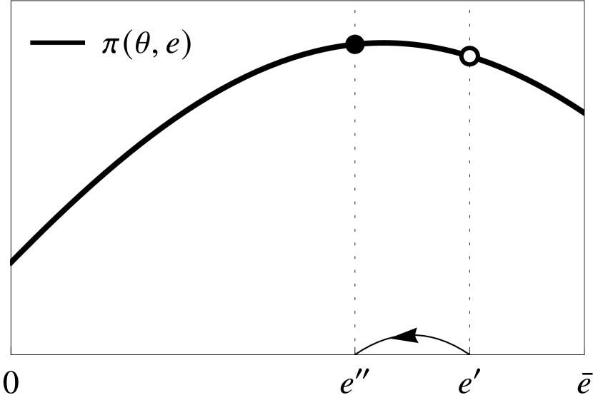
(a) Transparency decreases emission

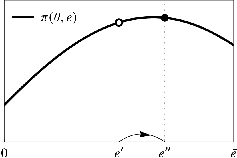
(b) Transparency increases emission

Figure 1: Both figures illustrate the effect of increasing transparency from a disclosure policy represented by the partition $\{[0,e^{\prime}],(e^{\prime},\bar{e}]\}$. This policy induces an equilibrium emission level $e^{\prime}$, as it yields a higher profit than the other belief-compatible emission level $\bar{e}$. In Figure 1(a), transparency is increased by breaking $[0,e^{\prime}]$ into intervals $[0,e^{\prime\prime}]$ and $(e^{\prime\prime},e^{\prime}]$, which leads to a lower equilibrium emission level $e^{\prime\prime}$. In Figure 1(b), transparency is increased by breaking $(e^{\prime},\bar{e}]$ into intervals $(e^{\prime},e^{\prime\prime}]$ and $(e^{\prime\prime},\bar{e}]$, which leads a higher equilibrium emission level $e^{\prime\prime}$.

In terms of the firm’s profit, the above argument reveals an even more striking observation: increased transparency never makes the firm worse off. The reason is simply that a more transparent disclosure policy enlarges the set of belief-compatible emission levels, which serves as the feasible set of the firm’s optimization problem. Intuitively, disclosure policies facilitate monitoring, and more transparent policies allow a larger set of emission levels to be communicated to the market. Unsurprisingly, the firm would then opt for the one in its favor, rather than being concerned about the resulting externality. I summarize this observation formally as follows.

Lemma 3.

If $d$ is more transparent than $d^{\prime}$, then $\pi_{d}(\theta)\geq\pi_{d^{\prime}}(\theta)$ for all $\theta\in\Theta$.

Proof.

Since $d$ is more transparent than $d^{\prime}$, we have $d^{\prime}(E)\subset d(E)$, which implies $\gamma_{d^{\prime}}(\theta)\in d(E)$ and thus the emission level $\gamma_{d^{\prime}}(\theta)$ is belief-compatible under policy $d$. Then we must have $\pi_{d}(\theta)=\pi(\theta,\gamma_{d}(\theta))\geq\pi(\theta,\gamma_{d^{\prime}}(\theta))=\pi_{d^{\prime}}(\theta)$. Because if this is not the case, the firm would receive a higher profit by deviating from $\gamma_{d}(\theta)$ to $\gamma_{d^{\prime}}(\theta)$ under policy $d$. ∎

4.2 Second Best

From now on, I return to the initial setting in which the energy efficiency level $\theta$ is the firm’s private information. The uncertainty of $\theta$ make it challenging, if not impossible, for the regulator to identify a single level of emission that maximizes social welfare. As a result, the optimal disclosure under asymmetric information may entail higher transparency than a binary form of disclosure as in the first best.

Increasing transparency tends to raise the firm’s expected profit, as it holds type by type by Lemma 3. This result may be considered as an argument in favor of transparency, provided the regulator values the firm’s private benefit along with emission reduction. Nonetheless, a more fundamental rationale for transparency lies in its impact on externalities under adverse selection. By choosing a disclosure policy, the regulator essentially offers the firm a menu of belief-compatible emission levels, with the maximal level $\bar{e}$ included by default so as to respect the individual rationality constraint. Depending on the firm’s type distribution, the regulator might want to offer a richer menu, by employing a more transparent policy, to screen the firm’s type more effectively. In light of this, increased transparency might be preferable for internalizing externalities, largely because it mitigates adverse selection, rather than moral hazard as suggested by conventional wisdom.

Nevertheless, transparency might as well exacerbate adverse selection through the transparency versus externality trade-off. While a more transparent disclosure policy may induce certain types of firms to lower their emissions, it might still raise the expected emissions, as some other types find it profitable to switch to higher levels of belief-compatible emissions made available by the increased transparency. Overall, the effect of transparency on emissions depends on the firm’s type distribution, as well as the region where transparency is increased. The non-monotonic relationship between transparency and emission discussed earlier continues to hold under asymmetric information.

4.3 Welfare Analysis

Having examined the impact of transparency on emissions and the firm’s profit, I will now turn to its welfare implications.

Definition 5 (Efficient Policy).

A disclosure policy $d$ is (ex ante) efficient if there is no disclosure policy $d^{\prime}\in\mathcal{D}$ such that $\Pi(d^{\prime})\geq\Pi(d)$ and $\Gamma(d^{\prime})\leq\Gamma(d)$, with at least one inequality strict.

The uninformative disclosure, or equivalently no disclosure, is clearly not efficient. In fact, it is the least efficient policy in the following sense.

Proposition 2 (No Disclosure).

The uninformative disclosure policy induces the highest emission level and the lowest profit among all disclosure policies.

Proof.

The uninformative disclosure, i.e., $d(e)=\bar{e}$ for all $e\in E$, induces the emission level $\bar{e}$ for all $\theta\in\Theta$. Therefore $\Gamma(d)=\bar{e}\geq\Gamma(d^{\prime})$ for all $d^{\prime}\in\mathcal{D}$. The claim on the expected profit follows from the inequality (IR) in Lemma 2. ∎

The uninformative disclosure can be thought of as the least transparent policy. On the other end of the spectrum, we have the most transparent disclosure policy defined as follows.

Definition 6 (Full Disclsoure).

A disclosure policy $d$ is a full-disclosure policy if $d(e)=e$ for all $e\in[\hat{\mathbf{e}}(\underline{\theta}),\hat{\mathbf{e}}(\bar{\theta})]$, where $\hat{\mathbf{e}}(\theta)\coloneqq\operatorname*{arg\,max}_{e\in E}\pi(\theta,e)$.

Since all the most desirable emission levels become observable to the market, under full disclosure each type $\theta$ is able to attain its highest possible equilibrium profit by choosing its most preferred emission level $\hat{\mathbf{e}}(\theta)$.

As the profit is maximized type by type under full disclosure, we are able to conclude the following.

Proposition 3.

A full-disclosure policy is efficient, and induces the highest expected profit among all disclosure policies.

Proof.

The claim on the expected profit follows directly from Lemma 3. Efficiency then follows from the strict concavity of $\pi(\theta,\cdot)$, which implies there does not exist a disclosure policy that attains a lower expected emission without lowering the expected profit. ∎

Given the non-monotonic relationship between transparency and emission as a result of the transparency versus externality trade-off, should the regulator seek more transparent disclosure policies to combat carbon emissions? The next proposition provides a partial answer.

Proposition 4.

If $d^{\prime}$ is more transparent than $d$ and $d$ is efficient, then $\Gamma(d^{\prime})\geq\Gamma(d)$.

Proof.

Given that $d^{\prime}$ is more transparent than $d$, Lemma 3 implies that $\Pi(d^{\prime})\geq\Pi(d)$. If $\Gamma(d^{\prime})<\Gamma(d)$, then by definition $d$ is not efficient, which is a contradiction. ∎

Starting with no disclosure, more transparent disclosures improve efficiency by mitigating the moral hazard problem. As long as inefficiency remains, the firm would embrace, rather than resist, the emission reduction induced by increased transparency because of the higher profit attained. Nonetheless, since more transparent disclosures tend to allocate the surplus to the firm, transparency exacerbates the externality once efficiency is achieved. Proposition 4 asserts that as long as efficiency is achieved, attempting to further reduce emissions by pursuing transparency would be in vain. This insight naturally leads to the following counterintuitive statement.

Proposition 5.

A full-disclosure policy induces the highest expected emission level among all efficient disclosure policies.

Proof.

This proposition follows directly from Proposition 4. ∎

Proposition 5 makes clear what would be achieved when pursuing maximal transparency. We learn from Lemma 3 and Proposition 3 that full transparency maximizes the profit of the firm and therefore restores efficiency. However, when efficiency is considered as a precondition for disclosure policies, perhaps surprisingly, full transparency proves to be the worst in terms of internalizing externalities.

5 Optimal Policy

In principle, an optimal solution to the disclosure problem can exhibit complex structures that divide the emission space into a mixture of multiple transparent and opaque regions. Nevertheless, I now show that optimal disclosure policies can take a rather simple structure, and provide sufficient conditions for this to occur. Specifically, I first restrict attention to a class of disclosure policies that exhibit the following threshold structure.

Definition 7 (Threshold Disclosure Policies).

A disclosure policy $d$ is said to be a threshold policy with threshold $e^{*}\in E$ if $d(e)=e$ for $e\leq e^{*}$ and $d(e)=\bar{e}$ otherwise.

A threshold policy thus contains a transparent region at the bottom and an opaque region at the top. For any threshold policy with threshold $e^{*}$, the induced equilibrium emission scheme $\mathbf{e}$ can be written as

$$\mathbf{e}(\theta)=\begin{cases}\hat{\mathbf{e}}(\theta);&\theta\leq\hat{\theta},\\ e^{*};&\theta\in(\hat{\theta},\theta^{*}],\\ \bar{e};&\theta\in(\theta^{*},\bar{\theta}],\end{cases}$$

where

$$\hat{\theta}\coloneqq\begin{cases}\bar{\theta};&\text{if }e^{*}>\hat{\mathbf{e}}(\bar{\theta}),\\ \hat{\mathbf{e}}^{-1}(e^{*});&\text{if }e^{*}\in[\hat{\mathbf{e}}(\underline{\theta}),\hat{\mathbf{e}}(\bar{\theta})],\\ \underline{\theta};&\text{if }e^{*}<\hat{\mathbf{e}}(\underline{\theta}),\end{cases}$$ (1)

and

$$\theta^{*}\coloneqq\begin{cases}\bar{\theta};&\text{if }e^{*}>\underline{\mathbf{e}}(\bar{\theta}),\\ \underline{\mathbf{e}}^{-1}(e^{*});&\text{if }e^{*}\in[\underline{\mathbf{e}}(\underline{\theta}),\underline{\mathbf{e}}(\bar{\theta})],\\ \underline{\theta};&\text{if }e^{*}<\underline{\mathbf{e}}(\underline{\theta}).\end{cases}$$ (2)

Figure 2 illustrates an example of the emission scheme implemented by a threshold policy. Firms with type $\theta\in[\underline{\theta},\hat{\theta})$ have $\hat{\mathbf{e}}(\theta)\leq e^{*}$, and thus are induced to choose their most preferred emission level $\hat{\mathbf{e}}(\theta)$. Firms with type $\theta\in[\hat{\theta},\theta^{*}]$ face $\pi(\theta,e^{*})\geq\pi(\theta,\bar{e})$. They are induced to lower their emission to the threshold $e^{*}$ since all emissions higher than $e^{*}$ will be pooled to $\bar{e}$. Lastly, firms with type $\theta\in(\theta^{*},\bar{\theta}]$ are those with $\pi(\theta,e^{*})<\pi(\theta,\bar{e})$ and thus do not find it worthwhile to reduce emissions from $\bar{e}$.

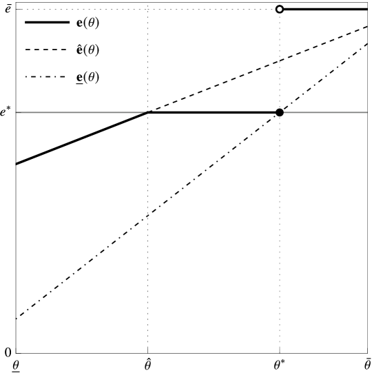
Figure 2: The emission scheme $\mathbf{e}(\theta)$ induced by a threshold policy with threshold $e^{*}$.

In general, solutions to the disclosure problem do not have to take the form of threshold policies described above. The next lemma establishes a sufficient condition under which a threshold policy solves the disclosure problem.

Lemma 4 (Optimality of Threshold Policies).

If $(1-\alpha)F(\theta)+\alpha f(\theta)$ is quasi-concave on $\Theta$, then a threshold policy solves the disclosure problem.

Proof.

See the Appendix. ∎

When the function $(1-\alpha)F(\theta)+\alpha f(\theta)$ is quasi-concave, Lemma 4 simplifies the disclosure problem to the choice of an optimal threshold—a straightforward univariate optimization problem. If, in addition, the function $(1-\alpha)F(\theta)+\alpha f(\theta)$ is strictly quasi-concave, then the optimal threshold is unique in $[0,\hat{\mathbf{e}}(\bar{\theta})]$. The strict quasi-concavity of this function is guaranteed for all $\alpha\in[0,1]$ if the density of the type distribution is strictly log-concave. This observation leads to the following proposition.

Proposition 6.

Suppose $f$ is continuously differentiable and $\ln(f(\theta))^{\prime\prime}<0$ on $\operatorname{\mathrm{int}}\Theta$. For each $\alpha\in[0,1]$, there is a unique $e^{*}\in[0,\hat{\mathbf{e}}(\bar{\theta})]$ such that the threshold policy with threshold $e^{*}$ solves the disclosure problem. This threshold is weakly decreasing in $\alpha$.

Proof.

See the Appendix. ∎

We learn from Proposition 5 that a full-disclosure policy induces the highest expected emission among all efficient policies, which suggests that full disclosure is more likely to be optimal if the regulator assigns a lower weight to the public benefit. It is worth noting that full disclosure can still be optimal for $\alpha>0$. In fact, it can even be optimal regardless of the weight $\alpha$, which occurs when all other disclosure policies are inefficient. The next proposition establishes the necessary and sufficient conditions for the optimality of full disclosure.

Proposition 7 (Optimality of Full Disclosure).

A full-disclosure policy is optimal for $\alpha$ if and only if

1. $\hat{\mathbf{e}}(\bar{\theta})=\bar{e}$ and $(1-\alpha)F(\theta)+\alpha f(\theta)$ is nondecreasing on $[\underline{\theta},\bar{\theta}]$,

2. or, $\alpha=0$.

Proof.

See the Appendix. ∎

As apparent from Proposition 7, if full disclosure is optimal for some $\alpha$, then it remains optimal for all weights smaller than $\alpha$.

Appendix A Proof of Lemma 2

Proof.

Suppose that $\mathbf{e}$ is implemented by $d$. Then we have

$$\tilde{\pi}(\theta,\mathbf{e}(\theta),d(\mathbf{e}(\theta)))\geq\tilde{\pi}(\theta,e^{\prime},d(e^{\prime}))$$ (3)

for all $\theta\in\Theta$ and $e^{\prime}\in E$. In particular for $e^{\prime}=\mathbf{e}(\theta^{\prime})$, inequality (3) becomes

$$\tilde{\pi}(\theta,\mathbf{e}(\theta),d(\mathbf{e}(\theta)))\geq\tilde{\pi}(\theta,\mathbf{e}(\theta^{\prime}),d(\mathbf{e}(\theta^{\prime}))).$$

This inequality, together with Lemma 1, gives

$$\pi(\theta,\mathbf{e}(\theta)) =\tilde{\pi}(\theta,\mathbf{e}(\theta),\mathbf{e}(\theta))$$

$$=\tilde{\pi}(\theta,\mathbf{e}(\theta),d(\mathbf{e}(\theta)))$$

$$\geq\tilde{\pi}(\theta,\mathbf{e}(\theta^{\prime}),d(\mathbf{e}(\theta^{\prime})))$$

$$=\tilde{\pi}(\theta,\mathbf{e}(\theta^{\prime}),\mathbf{e}(\theta^{\prime}))$$

$$=\pi(\theta,\mathbf{e}(\theta^{\prime})),$$

which yields inequality (IC).

Moreover, inequality (3) holds for $e^{\prime}=\bar{e}$, which, together with Lemma 1, gives

$$\pi(\theta,\mathbf{e}(\theta)) =\tilde{\pi}(\theta,\mathbf{e}(\theta),\mathbf{e}(\theta))$$

$$=\tilde{\pi}(\theta,\mathbf{e}(\theta),d(\mathbf{e}(\theta)))$$

$$\geq\tilde{\pi}(\theta,\bar{e},d(\bar{e}))$$

$$=\tilde{\pi}(\theta,\bar{e},\bar{e})$$

$$=\pi(\theta,\bar{e}),$$

which yields inequality (IR).

Now suppose that (IC) and (IR) hold. Let $d(e)=e$ if $e=\mathbf{e}(\theta)$ for some $\theta\in\Theta$, and $d(e)=\bar{e}$ otherwise. Consider any $e^{\prime}\in E$.

Suppose $e^{\prime}=\mathbf{e}(\theta^{\prime})$ for some $\theta^{\prime}\in\Theta$. Then for all $\theta^{\prime}\in\Theta$, we have

$$\tilde{\pi}(\theta,\mathbf{e}(\theta),d(\mathbf{e}(\theta))) =\tilde{\pi}(\theta,\mathbf{e}(\theta),\mathbf{e}(\theta))$$

$$\geq\tilde{\pi}(\theta,\mathbf{e}(\theta^{\prime}),\mathbf{e}(\theta^{\prime}))$$

$$=\tilde{\pi}(\theta,e^{\prime},e^{\prime})$$

$$=\tilde{\pi}(\theta,e^{\prime},d(e^{\prime})),$$

where the inequality comes from (IC).

Otherwise, if $e^{\prime}\neq\mathbf{e}(\theta)$ for any $\theta\in\Theta$, then for all $\theta^{\prime}\in\Theta$, we have

$$\tilde{\pi}(\theta,\mathbf{e}(\theta),d(\mathbf{e}(\theta))) =\tilde{\pi}(\theta,\mathbf{e}(\theta),\mathbf{e}(\theta))$$

$$\geq\tilde{\pi}(\theta,\bar{e},\bar{e})$$

$$\geq\tilde{\pi}(\theta,e^{\prime},\bar{e})$$

$$=\tilde{\pi}(\theta,e^{\prime},d(e^{\prime})),$$

where the first inequality comes from (IR), and the second inequality comes from the monotonicity of $\tilde{\pi}(\theta,\,\cdot\,,\tilde{e})$. Hence, $\mathbf{e}$ is implemented by $d$. ∎

Appendix B Proof of Lemma 4

First, the disclosure problem can be rewritten as

$$\max_{\mathbf{e}} \int_{\underline{\theta}}^{\bar{\theta}}[-\alpha\mathbf{e}(\theta)+(1-\alpha)\pi(\theta,\mathbf{e}(\theta))]\differential{F(\theta)}\quad\text{subject to:}$$

$$\pi(\theta,\mathbf{e}(\theta))+\int_{\theta}^{\bar{\theta}}\mathbf{e}(\tilde{\theta})\differential{\tilde{\theta}}=\pi(\bar{\theta},\mathbf{e}(\bar{\theta})),\quad\text{for all }\theta\in\Theta,$$

$$\pi(\theta,\mathbf{e}(\theta))\geq\pi(\theta,\bar{e}),\quad\text{for all }\theta\in\Theta,$$

$$\mathbf{e}:\Theta\to E\text{ nondecreasing}.$$

Next, I follow [1] and write the incentive constraint as two inequalities:

$$-\int_{\theta}^{\bar{\theta}}\mathbf{e}(\tilde{\theta})\differential{\tilde{\theta}}-\pi(\theta,\mathbf{e}(\theta))+\pi(\bar{\theta},\mathbf{e}(\bar{\theta})) \leq 0\quad\text{for all }\theta\in\Theta,$$

$$\int_{\theta}^{\bar{\theta}}\mathbf{e}(\tilde{\theta})\differential{\tilde{\theta}}+\pi(\theta,\mathbf{e}(\theta))-\pi(\bar{\theta},\mathbf{e}(\bar{\theta})) \leq 0\quad\text{for all }\theta\in\Theta.$$

With the choice set for $\mathbf{e}$ defined as $\Phi\coloneqq\{\mathbf{e}\mid\mathbf{e}:\Theta\to E,\text{ and }\mathbf{e}\text{ nondecreasing}\}$, the disclosure problem can further be written as

$$\max_{\mathbf{e}\in\Phi} \int_{\underline{\theta}}^{\bar{\theta}}[-\alpha\mathbf{e}(\theta)+(1-\alpha)\pi(\theta,\mathbf{e}(\theta))]\differential{F(\theta)}\quad\text{subject to:}$$

$$-\int_{\theta}^{\bar{\theta}}\mathbf{e}(\tilde{\theta})\differential{\tilde{\theta}}-\pi(\theta,\mathbf{e}(\theta))+\pi(\bar{\theta},\mathbf{e}(\bar{\theta}))\leq 0\quad\text{for all }\theta\in\Theta,$$ (4)

$$\int_{\theta}^{\bar{\theta}}\mathbf{e}(\tilde{\theta})\differential{\tilde{\theta}}+\pi(\theta,\mathbf{e}(\theta))-\pi(\bar{\theta},\mathbf{e}(\bar{\theta}))\leq 0\quad\text{for all }\theta\in\Theta,$$ (5)

$$-\pi(\theta,\mathbf{e}(\theta))+\pi(\theta,\bar{e})\leq 0\quad\text{for all }\theta\in\Theta.$$ (6)

Now, consider a threshold policy that is optimal within the class of all threshold policies. Denote by $\mathbf{e}^{*}$ the resulting emission scheme and by $e^{*}$ the associated threshold. Without loss of generality, I assume that $e^{*}\leq\hat{\mathbf{e}}(\bar{\theta})$, which implies that $\hat{\theta}=\bar{\theta}$ if and only if $e^{*}=\hat{\mathbf{e}}(\bar{\theta})$. In what follows, I show that $\mathbf{e}^{*}$ solves the optimization problem above.

Let $\Lambda_{1}(\theta)$, $\Lambda_{2}(\theta)$, and $\Psi(\theta)$ denote the (cumulative) multiplier functions associated with inequalities (4), (5) and (6), respectively. These functions are restricted to be nondecreasing on $\Theta$. Let $\Lambda(\theta)\coloneqq\Lambda_{1}(\theta)-\Lambda_{2}(\theta)$. The Lagrangian can be written as follows:

$$\mathcal{L}(\mathbf{e}\mid\Lambda,\Psi)= \int_{\underline{\theta}}^{\bar{\theta}}[-\alpha\mathbf{e}(\theta)+(1-\alpha)\pi(\theta,\mathbf{e}(\theta))]\differential{F(\theta)}$$

$$+\int_{\underline{\theta}}^{\bar{\theta}}\left(\int_{\theta}^{\bar{\theta}}\mathbf{e}(\tilde{\theta})\differential{\tilde{\theta}}+\pi(\theta,\mathbf{e}(\theta))-\pi(\bar{\theta},\mathbf{e}(\bar{\theta}))\right)\differential{\Lambda(\theta)}$$

$$+\int_{\underline{\theta}}^{\bar{\theta}}(\pi(\theta,\mathbf{e}(\theta))-\pi(\theta,\bar{e}))\differential{\Psi(\theta)}.$$

Integration by parts gives

$$\mathcal{L}(\mathbf{e}\mid\Lambda,\Psi)= \int_{\underline{\theta}}^{\bar{\theta}}-\alpha\mathbf{e}(\theta)\differential{F(\theta)}+\int_{\underline{\theta}}^{\bar{\theta}}\pi(\theta,\mathbf{e}(\theta))\differential{((1-\alpha)F(\theta)+\Lambda(\theta)+\Psi(\theta))}$$

$$+\int_{\underline{\theta}}^{\bar{\theta}}(\Lambda(\theta)-\Lambda(\underline{\theta}))\mathbf{e}(\theta)\differential{\theta}-\pi(\bar{\theta},\mathbf{e}(\bar{\theta}))(\Lambda(\bar{\theta})-\Lambda(\underline{\theta}))$$

$$-\int_{\underline{\theta}}^{\bar{\theta}}\pi(\theta,\bar{e})\differential{\Psi(\theta)}.$$

I propose the following multipliers:

$$\Lambda(\theta)\coloneqq\begin{cases}0,&\theta=\underline{\theta},\\ \alpha f(\theta),&\theta\in(\underline{\theta},\hat{\theta}),\\ (1-\alpha)F(\theta^{*})+\alpha f(\theta^{*})-(1-\alpha)F(\theta),&\theta\in[\hat{\theta},\theta^{*})\backslash\{\underline{\theta}\},\\ \alpha f(\theta),&\theta\in[\theta^{*},\bar{\theta}),\\ \alpha f(\theta^{*})-A,&\theta=\bar{\theta},\end{cases}$$

and

$$\Psi(\theta)\coloneqq\begin{cases}0,&\theta\in[\underline{\theta},\theta^{*}),\\ (1-\alpha)F(\theta^{*})+\alpha f(\theta^{*})-(1-\alpha)F(\theta)-\alpha f(\theta),&\theta\in[\theta^{*},\bar{\theta}),\\ (1-\alpha)F(\theta^{*})-(1-\alpha)F(\bar{\theta})+A,&\theta=\bar{\theta},\end{cases}$$

where

$$A\coloneqq\begin{cases}\frac{-1}{\pi_{e}(\theta^{*},e^{*})}\int_{\hat{\theta}}^{\theta^{*}}[-\alpha+(1-\alpha)\pi_{e}(\theta,e^{*})]\differential{F(\theta)},&\text{if }\pi_{e}(\theta^{*},e^{*})\neq 0\\ 0,&\text{otherwise}.\end{cases}$$

Note that these functions are well defined even if $\underline{\theta}=\hat{\theta}$ or $\theta^{*}=\bar{\theta}$. Also, note that we must have $e^{*}>\underline{\mathbf{e}}(\underline{\theta})$, which implies $\theta^{*}>\underline{\theta}$. Because if otherwise, the induced emission scheme becomes $\mathbf{e}^{*}(\theta)=\bar{e}$ for all $\theta\in\Theta$, which is clearly not optimal within the class of threshold policies.

By Lemma 5, we have $A=\alpha f(\theta^{*})$ if $\theta^{*}<\bar{\theta}$, and $A\in[0,\alpha f(\theta^{*})]$ otherwise. Therefore, if $\Psi(\theta)$ is discontinuous at $\bar{\theta}-$, then its jump at $\bar{\theta}$ cannot be negative. Moreover, since the function $(1-\alpha)F(\theta)+\alpha f(\theta)$ is quasi-concave, Lemma 6 implies that it is nonincreasing on $[\theta^{*},\bar{\theta}]$. Therefore, $\Psi$ is nondecreasing on $\Theta$. By letting $\Lambda_{1}(\theta)\coloneqq(1-\alpha)F(\theta)+\Lambda(\theta)+\Psi(\theta)$, and $\Lambda_{2}\coloneqq(1-\alpha)F(\theta)+\Psi(\theta)$, we will see that the function $\Lambda$ can be written as the difference between two nondecreasing functions, where the monotonicity of $\Lambda_{1}$ will be verified shortly.

With $\Lambda(\underline{\theta})=0$, the Lagrangian becomes

$$\mathcal{L}(\mathbf{e}\mid\Lambda,\Psi)= \int_{\underline{\theta}}^{\bar{\theta}}-\alpha\mathbf{e}(\theta)\differential{F(\theta)}+\int_{\underline{\theta}}^{\bar{\theta}}\pi(\theta,\mathbf{e}(\theta))\differential{((1-\alpha)F(\theta)+\Lambda(\theta)+\Psi(\theta))}$$

$$+\int_{\underline{\theta}}^{\bar{\theta}}\Lambda(\theta)\mathbf{e}(\theta)\differential{\theta}-\int_{\underline{\theta}}^{\bar{\theta}}\pi(\theta,\bar{e})\differential{\Psi(\theta)}-\Lambda(\bar{\theta})\pi(\bar{\theta},\mathbf{e}(\bar{\theta})).$$

Concavity of the Lagrangian

Since $\pi(\theta,e)$ is concave in $e$, the Lagrangian is concave in $\mathbf{e}$ if $(1-\alpha)F(\theta)+\Lambda(\theta)+\Psi(\theta)$ is nondecreasing in $\theta$. With the proposed multipliers, we have

$$(1-\alpha)F(\theta)+\Lambda(\theta)+\Psi(\theta)=\begin{cases}0,&\theta=\underline{\theta},\\ (1-\alpha)F(\theta)+\alpha f(\theta),&\theta\in(\underline{\theta},\hat{\theta}),\\ (1-\alpha)F(\theta^{*})+\alpha f(\theta^{*}),&\theta\in[\hat{\theta},\bar{\theta}]\backslash\{\underline{\theta}\}.\end{cases}$$

This expression is clearly nondecreasing if $\hat{\theta}=\underline{\theta}$. Now suppose that $\hat{\theta}>\underline{\theta}$. As the function $(1-\alpha)F(\theta)+\alpha f(\theta)$ is assumed to be quasi-concave, Lemma 6 implies that it is nondecreasing on $(\underline{\theta},\hat{\theta})$. Then, the above expression is nondecreasing on $\Theta$ as long as it has a nonnegative jump at $\hat{\theta}$. This is clearly the case if $\hat{\theta}=\theta^{*}=\bar{\theta}$. I will verify this fact later for the case of $\underline{\theta}<\hat{\theta}<\bar{\theta}$.

Maximizing the Lagrangian

I now show that the emission scheme $\mathbf{e}^{*}$ maximizes the Lagrangian. I first extend $\pi(\theta,\cdot)$ to the entire positive ray of the real line by defining

$$\hat{\pi}(\theta,e)\coloneqq\begin{cases}\pi(\theta,e),&\text{for }e\in[0,\bar{e}],\\ \pi(\theta,\bar{e})+\pi_{e}(\theta,\bar{e})(e-\bar{e}),&\text{for }e\in(\bar{e},\infty),\end{cases}$$

for all $\theta\in\Theta$. Consequently, the choice set $\Phi$ can be extended to a convex cone $\hat{\Phi}\coloneqq\{\mathbf{e}\mid\mathbf{e}:\Theta\to\mathbb{R}_{+},\text{ and }\mathbf{e}\text{ nondecreasing}\}$. I then define the extended Lagrangian as

$$\hat{\mathcal{L}}(\mathbf{e}\mid\Lambda,\Psi)= \int_{\underline{\theta}}^{\bar{\theta}}-\alpha\mathbf{e}(\theta)\differential{F(\theta)}+\int_{\underline{\theta}}^{\bar{\theta}}\hat{\pi}(\theta,\mathbf{e}(\theta))\differential{((1-\alpha)F(\theta)+\Lambda(\theta)+\Psi(\theta))}$$

$$+\int_{\underline{\theta}}^{\bar{\theta}}\Lambda(\theta)\mathbf{e}(\theta)\differential{\theta}-\int_{\underline{\theta}}^{\bar{\theta}}\hat{\pi}(\theta,\bar{e})\differential{\Psi(\theta)}-\Lambda(\bar{\theta})\hat{\pi}(\bar{\theta},\mathbf{e}(\bar{\theta})).$$

For the same reason as before, $\hat{\mathcal{L}}$ is concave in $\mathbf{e}$. Moreover, because $\hat{\mathcal{L}}$ and $\mathcal{L}$ coincide on $\Phi$, I can say that if $\mathbf{e}^{*}$ maximizes the extended Lagrangian $\hat{\mathcal{L}}(\mathbf{e}\mid\Lambda,\Psi)$ over $\hat{\Phi}$, then it also maximizes Lagrangian $\mathcal{L}(\mathbf{e}\mid\Lambda,\Psi)$ over $\Phi$. According to Lemma A.2 in [3], I can then say that if

$$\partial\hat{\mathcal{L}}(\mathbf{e}^{*};\mathbf{e}^{*}\mid\Lambda,\Psi)=0,$$

$$\partial\hat{\mathcal{L}}(\mathbf{e}^{*};\mathbf{x}\mid\Lambda,\Psi)\leq 0;\quad\text{for all }\mathbf{x}\in\hat{\Phi},$$

then $\mathbf{e}^{*}$ maximizes $\hat{\mathcal{L}}(\mathbf{e}\mid\Lambda,\Psi)$ over $\hat{\Phi}$. In what follows, I show that these conditions are satisfied.

Taking the Gateaux differential in the direction $\mathbf{x}\in\hat{\Phi}$, we have

$$\partial{\hat{\mathcal{L}}(\mathbf{e}^{*};\mathbf{x}\mid\Lambda,\Psi)}= \int_{\underline{\theta}}^{\bar{\theta}}\left[-\alpha f(\theta)+\Lambda(\theta)\right]\mathbf{x}(\theta)\differential{\theta}$$

$$+\int_{\underline{\theta}}^{\bar{\theta}}\pi_{e}(\theta,\mathbf{e}^{*}(\theta))\mathbf{x}(\theta)\differential{((1-\alpha)F(\theta)+\Lambda(\theta)+\Psi(\theta))}$$

$$-\Lambda(\bar{\theta})\pi_{e}(\bar{\theta},\mathbf{e}^{*}(\bar{\theta}))\mathbf{x}(\bar{\theta}).$$

Given our choice of $\Lambda(\theta)$ within the interval $(\underline{\theta},\hat{\theta})$ and the observation that $\pi_{e}(\theta,\mathbf{e}^{*}(\theta))=\pi_{e}(\theta,\hat{\mathbf{e}}(\theta))=0$ for all $\theta\in[\underline{\theta},\hat{\theta}]$ whenever $\hat{\theta}>\underline{\theta}$, it follows that

$$\partial{\hat{\mathcal{L}}(\mathbf{e}^{*};\mathbf{x}\mid\Lambda,\Psi)}= \int_{\hat{\theta}}^{\bar{\theta}}\left[-\alpha f(\theta)+\Lambda(\theta)\right]\mathbf{x}(\theta)\differential{\theta}$$

$$+\int_{\hat{\theta}}^{\bar{\theta}}\pi_{e}(\theta,\mathbf{e}^{*}(\theta))\mathbf{x}(\theta)\differential{((1-\alpha)F(\theta)+\Lambda(\theta)+\Psi(\theta))}$$

$$-\Lambda(\bar{\theta})\pi_{e}(\bar{\theta},\mathbf{e}^{*}(\bar{\theta}))\mathbf{x}(\bar{\theta}).$$

Integration by parts yields

$$\partial{\hat{\mathcal{L}}(\mathbf{e}^{*};\mathbf{x}\mid\Lambda,\Psi)}= \left[\int_{\hat{\theta}}^{\bar{\theta}}\left[-\alpha f(\theta)+\Lambda(\theta)\right]\differential{\theta}\right.$$

$$\left.\quad+\int_{\hat{\theta}}^{\bar{\theta}}\pi_{e}(\theta,\mathbf{e}^{*}(\theta))\differential{((1-\alpha)F(\theta)+\Lambda(\theta)+\Psi(\theta))}\right]\mathbf{x}(\hat{\theta})$$

$$+\int_{\hat{\theta}}^{\bar{\theta}}\left[\int_{\theta}^{\bar{\theta}}[-\alpha f(\tilde{\theta})+\Lambda(\tilde{\theta})]\differential{\tilde{\theta}}\right.$$

$$\left.\quad\quad\quad+\int_{\theta}^{\bar{\theta}}\pi_{e}(\tilde{\theta},\mathbf{e}^{*}(\tilde{\theta}))\differential{((1-\alpha)F(\tilde{\theta})+\Lambda(\tilde{\theta})+\Psi(\tilde{\theta}))}\right]\differential{\mathbf{x}(\theta)}$$

$$-\Lambda(\bar{\theta})\pi_{e}(\bar{\theta},\mathbf{e}^{*}(\bar{\theta}))\mathbf{x}(\bar{\theta})$$

$$= Q(\hat{\theta})\mathbf{x}(\hat{\theta})-\Lambda(\bar{\theta})\pi_{e}(\bar{\theta},\mathbf{e}^{*}(\bar{\theta}))\mathbf{x}(\bar{\theta})+\int_{\hat{\theta}}^{\bar{\theta}}Q(\theta)\differential{\mathbf{x}(\theta)},$$

where I define

$$Q(\theta)\coloneqq\int_{\theta}^{\bar{\theta}}\left[-\alpha f(\tilde{\theta})+\Lambda(\tilde{\theta})\right]\differential{\tilde{\theta}}+\int_{\theta}^{\bar{\theta}}\pi_{e}(\tilde{\theta},\mathbf{e}^{*}(\tilde{\theta}))\differential{((1-\alpha)F(\tilde{\theta})+\Lambda(\tilde{\theta})+\Psi(\tilde{\theta}))}$$

for $\theta\in[\hat{\theta},\bar{\theta}]$.

Proof of $\partial{\hat{\mathcal{L}}(\mathbf{e}^{*};\mathbf{e}^{*}\mid\Lambda,\Psi)}=0$.

For $\mathbf{x}=\mathbf{e}^{*}$, we have

$$\partial{\hat{\mathcal{L}}(\mathbf{e}^{*};\mathbf{e}^{*}\mid\Lambda,\Psi)} =Q(\hat{\theta})\mathbf{e}^{*}(\hat{\theta})-\Lambda(\bar{\theta})\pi_{e}(\bar{\theta},\mathbf{e}^{*}(\bar{\theta}))\mathbf{e}^{*}(\bar{\theta})+\int_{\hat{\theta}}^{\bar{\theta}}Q(\theta)\differential{\mathbf{e}^{*}(\theta)}$$

$$=Q(\hat{\theta})\mathbf{e}^{*}(\hat{\theta})-\Lambda(\bar{\theta})\pi_{e}(\bar{\theta},\mathbf{e}^{*}(\bar{\theta}))\mathbf{e}^{*}(\bar{\theta})+Q(\theta^{*})(\bar{e}-e^{*}).$$

Next, I show that

$$Q(\theta^{*})=0,$$ (7)

and $$Q(\hat{\theta})\mathbf{e}^{*}(\hat{\theta})=\Lambda(\bar{\theta})\pi_{e}(\bar{\theta},\mathbf{e}^{*}(\bar{\theta}))\mathbf{e}^{*}(\bar{\theta}),$$ (8)

which gives $\partial{\hat{\mathcal{L}}(\mathbf{e}^{*};\mathbf{e}^{*}\mid\Lambda,\Psi)}=0$.

Since the function $(1-\alpha)F(\theta)+\Lambda(\theta)+\Psi(\theta)$ is constant over the interval $[\theta^{*},\bar{\theta}]$ and $\Lambda(\theta)=\alpha f(\theta)$ for $\theta\in(\theta^{*},\bar{\theta})$, it follows that

$$Q(\theta^{*}) =\int_{\theta^{*}}^{\bar{\theta}}\left[-\alpha f(\theta)+\Lambda(\theta)\right]\differential{\theta}$$

$$\quad+\int_{\theta^{*}}^{\bar{\theta}}\pi_{e}(\theta,\mathbf{e}^{*}(\theta))\differential{((1-\alpha)F(\theta)+\Lambda(\theta)+\Psi(\theta))}$$

$$=0,$$

which shows equality (7).

To show equality (8), we can write $Q(\hat{\theta})$ as

$$Q(\hat{\theta})=Q(\hat{\theta})-Q(\theta^{*})$$

$$=\int_{\hat{\theta}}^{\theta^{*}}[-\alpha f(\theta)+\Lambda(\theta)]\differential{\theta}+\int_{\hat{\theta}}^{\theta^{*}}\pi_{e}(\theta,\mathbf{e}^{*}(\theta))\differential{((1-\alpha)F(\theta)+\Lambda(\theta)+\Psi(\theta))}$$

$$=\int_{\hat{\theta}}^{\theta^{*}}[-\alpha f(\theta)+\Lambda(\theta)]\differential{\theta}+\int_{\hat{\theta}}^{\theta^{*}}\pi_{e}(\theta,e^{*})\differential{((1-\alpha)F(\theta)+\Lambda(\theta)+\Psi(\theta))}$$

$$=\int_{\hat{\theta}}^{\theta^{*}}[-\alpha+(1-\alpha)\pi_{e}(\theta,e^{*})]\differential{F(\theta)}+\int_{\hat{\theta}}^{\theta^{*}}\derivative{\theta}\left(\Lambda(\theta)\pi_{e}(\theta,e^{*})\right)\differential{\theta}+\int_{\hat{\theta}}^{\theta^{*}}\pi_{e}(\theta,e^{*})\differential{\Psi(\theta)}$$

$$=\int_{\hat{\theta}}^{\theta^{*}}[-\alpha+(1-\alpha)\pi_{e}(\theta,e^{*})]\differential{F(\theta)}+\underbrace{(\Lambda(\theta^{*})+\Psi(\theta^{*}))}_{=\alpha f(\theta^{*})}\pi_{e}(\theta^{*},e^{*})-\underbrace{\Lambda(\hat{\theta})\pi_{e}(\hat{\theta},e^{*})}_{=0}$$

$$=\int_{\hat{\theta}}^{\theta^{*}}[-\alpha+(1-\alpha)\pi_{e}(\theta,e^{*})]\differential{F(\theta)}+\alpha f(\theta^{*})\pi_{e}(\theta^{*},e^{*}),$$

where $\Lambda(\hat{\theta})\pi_{e}(\hat{\theta},e^{*})=0$ comes from the fact that $\pi_{e}(\hat{\theta},e^{*})=0$ if $\hat{\theta}>\underline{\theta}$ and $\Lambda(\hat{\theta})=0$ if $\hat{\theta}=\underline{\theta}$.

If $\theta^{*}<\bar{\theta}$, which occurs when $e^{*}<\underline{\mathbf{e}}(\bar{\theta})$, then by Lemma 5 we have both $\Lambda(\bar{\theta})=0$ and $Q(\hat{\theta})=0$, which yields equality (8). Otherwise, if $\theta^{*}=\bar{\theta}$, we have $\mathbf{e}^{*}(\hat{\theta})=\mathbf{e}^{*}(\bar{\theta})=e^{*}$. Then equality (8) follows from $Q(\hat{\theta})=\Lambda(\bar{\theta})\pi_{e}(\bar{\theta},e^{*})$, which holds by our choice of $\Lambda(\bar{\theta})$. Since both equalities (7) and (8) are satisfied, we have $\partial{\hat{\mathcal{L}}(\mathbf{e}^{*};\mathbf{e}^{*}\mid\Lambda,\Psi)}=0$.

Proof of $\partial{\hat{\mathcal{L}}(\mathbf{e}^{*};\mathbf{x}^{*}\mid\Lambda,\Psi)}\leq 0$ for all $\mathbf{x}\in\hat{\Phi}$.

I have shown $Q(\hat{\theta})=\Lambda(\bar{\theta})\pi_{e}(\bar{\theta},\mathbf{e}^{*}(\bar{\theta}))$ for both $\theta^{*}<\bar{\theta}$ and $\theta^{*}=\bar{\theta}$. Next, I show that $Q(\hat{\theta})\geq Q(\theta)$ for all $\theta\in[\hat{\theta},\bar{\theta}]$, which leads to

$$\partial{\hat{\mathcal{L}}(\mathbf{e}^{*};\mathbf{x}\mid\Lambda,\Psi)} =Q(\hat{\theta})\mathbf{x}(\hat{\theta})-\Lambda(\bar{\theta})\pi_{e}(\bar{\theta},\mathbf{e}^{*}(\bar{\theta}))\mathbf{x}(\bar{\theta})+\int_{\hat{\theta}}^{\bar{\theta}}Q(\theta)\differential{\mathbf{x}(\theta)}$$

$$=Q(\hat{\theta})(\mathbf{x}(\hat{\theta})-\mathbf{x}(\bar{\theta}))+\int_{\hat{\theta}}^{\bar{\theta}}Q(\theta)\differential{\mathbf{x}(\theta)}$$

$$\leq Q(\hat{\theta})(\mathbf{x}(\hat{\theta})-\mathbf{x}(\bar{\theta}))+Q(\hat{\theta})\int_{\hat{\theta}}^{\bar{\theta}}\differential{\mathbf{x}(\theta)}$$

$$=0.$$

Since the function $(1-\alpha)F(\theta)+\Lambda(\theta)+\Psi(\theta)$ is constant over the interval $[\theta^{*},\bar{\theta}]$, we have $Q(\theta)=0$ for all $\theta\in[\theta^{*},\bar{\theta}]$ by our choice of $\Lambda$. Moreover, we know from Lemma 5 that $Q(\hat{\theta})\geq 0$, and thus $Q(\hat{\theta})\geq Q(\theta)$ for all $\theta\in[\theta^{*},\bar{\theta}]$.

To show $Q(\hat{\theta})\geq Q(\theta)$ for all $\theta\in(\hat{\theta},\theta^{*})$, suppose by contradiction that $Q(\hat{\theta})<Q(\theta_{1})$ for some $\theta_{1}\in(\hat{\theta},\theta^{*})$.

By the definition of $Q$, we know that $Q(\theta^{*}-)=Q(\theta^{*})=0$, and $Q$ is continuously differentiable on $(\hat{\theta},\theta^{*})$, with

$$Q^{\prime}(\theta) =\alpha f(\theta)-\Lambda(\theta)$$

$$=(1-\alpha)F(\theta)+\alpha f(\theta)-(1-\alpha)F(\theta^{*})-\alpha f(\theta^{*}).$$

Since $Q(\theta_{1})>Q(\hat{\theta})\geq 0=Q(\theta^{*}-)$, we must have $Q^{\prime}(\theta_{2})<0=Q^{\prime}(\theta^{*}-)$ for some $\theta_{2}\in(\theta_{1},\theta^{*})$. Also, note that $Q^{\prime}$ is quasi-concave due to the quasi-concavity of the function $(1-\alpha)F(\theta)+\alpha f(\theta)$. This property of $Q^{\prime}$, together with the inequality $Q^{\prime}(\theta_{2})<Q^{\prime}(\theta^{*}-)$, implies that $Q^{\prime}$ must be nondecreasing on $(\hat{\theta},\theta_{2})$. Consequently, we have $Q^{\prime}(\theta)\leq Q^{\prime}(\theta_{1})\leq Q^{\prime}(\theta_{2})<0$ for all $\theta\in(\hat{\theta},\theta_{1})$. However, from the definition of $Q$ we can observe that $Q(\hat{\theta})\geq Q(\hat{\theta}+)$. Then, the fact that $Q^{\prime}(\theta)<0$ for all $\theta\in(\hat{\theta},\theta_{1})$ leads to $Q(\hat{\theta})\geq Q(\theta_{1})$, a contradiction.

Lastly, I return to my earlier claim that that the jump in $(1-\alpha)F(\theta)+\Lambda(\theta)+\Psi(\theta)$ at $\hat{\theta}$ is nonnegative when $\underline{\theta}<\hat{\theta}<\bar{\theta}$. I continue to validate this assertion by verifying the inequality

$$(1-\alpha)F(\theta^{*})+\alpha f(\theta^{*})\geq(1-\alpha)F(\hat{\theta})+\alpha f(\hat{\theta}).$$

From the definition of $Q$, we can observe that $Q$ is right-continuous at $\hat{\theta}$ if $\hat{\theta}>\underline{\theta}$. I have also shown that $Q(\hat{\theta})\geq Q(\theta)$ for all $\theta\in[\hat{\theta},\theta^{*}]$. Therefore, the right-hand derivative of $Q$ at $\hat{\theta}$ must be nonpositive, which gives

$$0 \geq Q^{\prime}(\hat{\theta}+)=(1-\alpha)F(\hat{\theta})+\alpha f(\hat{\theta})-(1-\alpha)F(\theta^{*})-\alpha f(\theta^{*}).$$

Therefore, if $\hat{\theta}>\underline{\theta}$, the jump in $(1-\alpha)F(\theta)+\Lambda(\theta)+\Psi(\theta)$ at $\hat{\theta}$ is nonnegative. As a result, the function $(1-\alpha)F(\theta)+\Lambda(\theta)+\Psi(\theta)$ is indeed nondecreasing on $\Theta$.

To summarize, I have shown that $\partial\hat{\mathcal{L}}(\mathbf{e}^{*};\mathbf{e}^{*}\mid\Lambda,\Psi)=0$ and $\partial\hat{\mathcal{L}}(\mathbf{e}^{*};\mathbf{x}\mid\Lambda,\Psi)\leq 0$ for all $\mathbf{x}\in\hat{\Phi}$. Therefore, according to Lemma A.2 in [3], I conclude that $\mathbf{e}^{*}$ maximizes $\hat{\mathcal{L}}$ over $\hat{\Phi}$, and thus also maximizes $\mathcal{L}$ over $\Phi$.

Applying Luenberger’s Sufficiency Theorem

Next, I apply Theorem 1 in [1], which is restated here for convenience.

Theorem 1 ([1], Theorem 1).

Let $f$ be a real-valued functional defined on a subset $\Omega$ of a linear space $X$. Let $G$ be a mapping from $\Omega$ into the linear space $Z$ having nonempty positive cone $P$. Suppose that

1. there exists a linear function $T:Z\to\mathbb{R}$ such that $T(z)\geq 0$ for all $z\in P$,

2. there is an element $x_{0}\in\Omega$ such that

   $$f(x_{0})+T(G(x_{0}))\leq f(x)+T(G(x))\quad\text{for all }x\in\Omega,$$

3. $-G(x_{0})\in P$, and

4. $T(G(x_{0}))=0$.

Then $x_{0}$ solves

$$\min f(x)\text{ subject to: }-G(x)\in P,x\in\Omega.$$

To apply this theorem, I set

1. $x_{0}\coloneqq\mathbf{e}^{*}$;

2. $X\coloneqq\{\mathbf{e}\mid\mathbf{e}:\Theta\to E\}$;

3. $f$ to be given by $-\int_{\underline{\theta}}^{\bar{\theta}}[-\alpha\mathbf{e}(\theta)+(1-\alpha)\pi(\theta,\mathbf{e}(\theta))]\differential{F(\theta)}$, as a function of $e\in X$;

4. $Z\coloneqq\{(z_{1},z_{2},z_{3})\mid z_{1}:\Theta\to\mathbb{R},z_{2}:\Theta\to\mathbb{R}\text{ and }z_{3}:\Theta\to\mathbb{R}\text{ with }z_{1},z_{2},z_{3}\text{ integrable}\}$;

5. $\Omega\coloneqq\Phi$;

6. $P\coloneqq\{(z_{1},z_{2},z_{3})\mid(z_{1},z_{2},z_{3})\in Z\text{ such that }z_{1}(\theta)\geq 0,z_{2}(\theta)\geq 0\text{ and }z_{3}(\theta)\geq 0\text{ for all }\theta\in\Theta\}$;

7. $G$ to be the mapping from $\Phi$ to $Z$ given by the left-hand sides of inequalities (4), (5) and (6);

8. $T$ to be the linear mapping:

   $$T((z_{1},z_{2},z_{3}))\coloneqq\int_{\Theta}z_{1}(\theta)\differential{\Lambda_{1}(\theta)}+\int_{\Theta}z_{2}(\theta)\differential{\Lambda_{2}(\theta)}+\int_{\Theta}z_{3}(\theta)\differential{\Psi(\theta)},$$

   where $\Lambda_{1}$, $\Lambda_{2}$, and $\Psi$ being nondecreasing functions implies that $T(z)\geq 0$ for $z\in P$.

We have that

$$T(G(x_{0})) =-\left[\int_{\Theta}\int_{\theta}^{\bar{\theta}}\pi_{\theta}(\tilde{\theta},\mathbf{e}^{*}(\tilde{\theta}))\differential{\theta}+\pi(\theta,\mathbf{e}^{*}(\theta))-\pi(\bar{\theta},\mathbf{e}^{*}(\bar{\theta}))\right]\differential{(\Lambda_{1}(\theta)-\Lambda_{2}(\theta))}$$

$$\quad-\int_{\Theta}(\pi(\theta,\mathbf{e}^{*}(\theta))-\pi(\theta,\bar{e}))\differential{\Psi(\theta)}$$

$$=0,$$

where the last equality follows from the construction of $\mathbf{e}^{*}$ and the proposed multipliers. We have found the conditions under which the proposed $\mathbf{e}^{*}$ minimizes $f(x)+T(G(x))$ for $x\in\Omega$. Given that $T(G(x_{0}))=0$, the conditions of Theorem 1 hold and it follows that $\mathbf{e}^{*}$ solves $\min_{x\in\Omega}f(x)$ subject to $-G(x)\in P$, which is the original problem.

Lemma 5.

Let $e^{*}$ be the threshold of a threshold policy that is optimal within the class of all threshold policies. Let $\hat{\theta}$ and $\theta^{*}$ defined as in (1) and (2). Then we have

$$-\int_{\hat{\theta}}^{\theta^{*}}[-\alpha+(1-\alpha)\pi_{e}(\theta,e^{*})]\differential{F(\theta)}\begin{cases}=\alpha f(\theta^{*})\pi_{e}(\theta^{*},e^{*}),&\text{ if }e^{*}<\underline{\mathbf{e}}(\bar{\theta}),\\ \in[0,\alpha f(\theta^{*})\pi_{e}(\theta^{*},e^{*})],&\text{ if }e^{*}=\underline{\mathbf{e}}(\bar{\theta}),\\ =0,&\text{ if }\underline{\mathbf{e}}(\bar{\theta})<e^{*}\leq\bar{e}.\end{cases}$$

Proof.

The expected welfare associated with such a threshold policy is given by

$$\int_{\underline{\theta}}^{\bar{\theta}}[-\alpha\mathbf{e}(\theta)+(1-\alpha)\pi(\theta,\mathbf{e}(\theta))]\differential{F(\theta)}$$

$$= \int_{\underline{\theta}}^{\hat{\theta}}[-\alpha\hat{\mathbf{e}}(\theta)+(1-\alpha)\pi(\theta,\hat{\mathbf{e}}(\theta))]\differential{F(\theta)}+\int_{\hat{\theta}}^{\theta^{*}}[-\alpha e^{*}+(1-\alpha)\pi(\theta,e^{*})]\differential{F(\theta)}$$

$$+\int_{\theta^{*}}^{\bar{\theta}}[-\alpha\bar{e}+(1-\alpha)\pi(\theta,\bar{e})]\differential{F(\theta)}.$$

Take derivative with respect to $e^{*}$, we have

$$[-\alpha e^{*}+(1-\alpha)\pi(\hat{\theta},e^{*})]f(\hat{\theta})\derivative{\hat{\theta}}{e^{*}}+[-\alpha e^{*}+(1-\alpha)\pi(\theta^{*},e^{*})]f(\theta^{*})\derivative{\theta^{*}}{e^{*}}$$

$$-[-\alpha e^{*}+(1-\alpha)\pi(\hat{\theta},e^{*})]f(\hat{\theta})\derivative{\hat{\theta}}{e^{*}}+\int_{\hat{\theta}}^{\theta^{*}}[-\alpha+(1-\alpha)\pi_{e}(\theta,e^{*})]\differential{F(\theta)}$$

$$-[-\alpha\bar{e}+(1-\alpha)\underbrace{\pi(\theta^{*},\bar{e})}_{=\pi(\theta^{*},e^{*})}]f(\theta^{*})\derivative{\theta^{*}}{e^{*}}$$

$$=\alpha(\bar{e}-e^{*})f(\theta^{*})\derivative{\theta^{*}}{e^{*}}+\int_{\hat{\theta}}^{\theta^{*}}[-\alpha+(1-\alpha)\pi_{e}(\theta,e^{*})]\differential{F(\theta)}.$$

1. If $e^{*}<\underline{\mathbf{e}}(\bar{\theta})$, then $\derivative{\theta^{*}}{e^{*}}=\frac{1}{\underline{\mathbf{e}}^{\prime}(\theta^{*})}$. By the definition of $\underline{\mathbf{e}}(\cdot)$ we have $\pi(\theta,\underline{\mathbf{e}}(\theta))=\pi(\theta,\bar{e})$. Taking derivative with respect to $\theta$ on both sides gives

   $$\pi_{\theta}(\theta,\underline{\mathbf{e}}(\theta))+\pi_{e}(\theta,\underline{\mathbf{e}}(\theta))\underline{\mathbf{e}}^{\prime}(\theta)=\pi_{\theta}(\theta,\bar{e}).$$

   Therefore, we have $\underline{\mathbf{e}}^{\prime}(\theta^{*})=(\bar{e}-e^{*})/\pi_{e}(\theta^{*},e^{*})$, and hence $\derivative{\theta^{*}}{e^{*}}=\frac{\pi_{e}(\theta^{*},e^{*})}{\bar{e}-e^{*}}$. Then, the first-order condition yields

   $$-\int_{\hat{\theta}}^{\theta^{*}}[-\alpha+(1-\alpha)\pi_{e}(\theta,e^{*})]\differential{F(\theta)}=\alpha f(\theta^{*})\pi_{e}(\theta^{*},e^{*}).$$

2. If $e^{*}=\underline{\mathbf{e}}(\bar{\theta})=\bar{e}$, then we have $\hat{\theta}=\theta^{*}=\bar{\theta}$, and hence

   $$-\int_{\hat{\theta}}^{\theta^{*}}[-\alpha+(1-\alpha)\pi_{e}(\theta,e^{*})]\differential{F(\theta)}=0\in[0,\alpha f(\theta^{*})\pi_{e}(\theta^{*},e^{*})].$$

3. If $e^{*}=\underline{\mathbf{e}}(\bar{\theta})<\bar{e}$, then the derivative of the expected welfare with respect to $e^{*}$ must be nonnegative as $e^{*}\uparrow\underline{\mathbf{e}}(\bar{\theta})$, which yields

   $$-\int_{\hat{\theta}}^{\theta^{*}}[-\alpha+(1-\alpha)\pi_{e}(\theta,e^{*})]\differential{F(\theta)}\leq\alpha f(\theta^{*})\pi_{e}(\theta^{*},e^{*}).$$

   Moreover, the derivative must also be nonpositive as $e^{*}\downarrow\underline{\mathbf{e}}(\bar{\theta})$. Because $\left.\derivative{\theta^{*}}{e^{*}}\right\rvert_{e^{*}=\underline{\mathbf{e}}(\bar{\theta})+}=0$, we have

   $$-\int_{\hat{\theta}}^{\theta^{*}}[-\alpha+(1-\alpha)\pi_{e}(\theta,e^{*})]\differential{F(\theta)}\geq 0.$$

4. Lastly, if $\underline{\mathbf{e}}(\bar{\theta})<\bar{e}$ and $e^{*}\in(\underline{\mathbf{e}}(\bar{\theta}),\bar{e}]$, then we have $\derivative{\theta^{*}}{e^{*}}=0$. The first-order condition then yields

   $$-\int_{\hat{\theta}}^{\theta^{*}}[-\alpha+(1-\alpha)\pi_{e}(\theta,e^{*})]\differential{F(\theta)}=0.$$

∎

Lemma 6.

Suppose $(1-\alpha)F(\theta)+\alpha f(\theta)$ is quasi-concave, and denote the set of its maximizers by $\Theta^{\blacktriangle}_{\alpha}\coloneqq\arg\max_{\theta\in\Theta}\{(1-\alpha)F(\theta)+\alpha f(\theta)\}$. If a threshold policy, with threshold $e^{*}$ and the associated $\hat{\theta}$ and $\theta^{*}$ defined as in (1) and (2), is optimal within the class of all threshold policies, then we have $[\hat{\theta},\theta^{*}]\cap\Theta^{\blacktriangle}_{\alpha}\neq\varnothing$.

Proof.

In this proof, I distinguish three cases.

Case 1: $e^{*}<\underline{\mathbf{e}}(\bar{\theta})$.

Since $e^{*}\leq\underline{\mathbf{e}}(\underline{\theta})$ is never optimal, in this case we are certain that $e^{*}\in(\underline{\mathbf{e}}(\underline{\theta}),\underline{\mathbf{e}}(\bar{\theta}))$. For an arbitrary threshold policies with threshold $e_{1}\in(\underline{\mathbf{e}}(\underline{\theta}),\underline{\mathbf{e}}(\bar{\theta}))$ and the corresponding $\hat{\theta}_{1}$ and $\theta^{*}_{1}$, the derivative of the expected welfare with respect to $e_{1}$ is given by

$$W^{\prime}(e_{1})= \int_{\hat{\theta}_{1}}^{\theta^{*}_{1}}[-\alpha+(1-\alpha)\pi_{e}(\theta,e_{1})]\differential{F(\theta)}+\alpha f(\theta^{*}_{1})\pi_{e}(\theta^{*}_{1},e_{1})$$

$$= \int_{\hat{\theta}_{1}}^{\theta^{*}_{1}}\pi_{e}(\theta,e_{1})\differential{((1-\alpha)F(\theta)+\alpha f(\theta))}+\alpha f(\hat{\theta}_{1})\pi_{e}(\hat{\theta}_{1},e_{1}).$$

At the optimal threshold $e^{*}$, the first-order condition yields

$$W^{\prime}(e^{*})=\int_{\hat{\theta}}^{\theta^{*}}\pi_{e}(\theta,e^{*})\differential{((1-\alpha)F(\theta)+\alpha f(\theta))}+\alpha f(\hat{\theta})\pi_{e}(\hat{\theta},e^{*})=0,$$

which implies

$$\int_{\hat{\theta}}^{\theta^{*}}\pi_{e}(\theta,e^{*})\differential{((1-\alpha)F(\theta)+\alpha f(\theta))}=-\alpha f(\hat{\theta})\pi_{e}(\hat{\theta},e^{*})\leq 0.$$

Now, suppose by contradiction that $[\hat{\theta},\theta^{*}]\cap\Theta^{\blacktriangle}_{\alpha}=\varnothing$. Then, the quasi-concave function $(1-\alpha)F(\theta)+\alpha f(\theta)$ must be either nondecreasing or nonincreasing on the interval $[\hat{\theta},\theta^{*}]$. Moreover, since $\pi_{e}(\theta,e^{*})>0$ on $(\hat{\theta},\theta^{*})$, the above inequality implies the function $(1-\alpha)F(\theta)+\alpha f(\theta)$ can only be nonincreasing on $[\hat{\theta},\theta^{*}]$. It must then follow that $(1-\alpha)F(\theta)+\alpha f(\theta)$ is constant on $[\hat{\theta},\theta^{*}]$. To see this, suppose by contradiction that this function contains a strictly decreasing part within $[\hat{\theta},\theta^{*}]$. Then the integral above has to be negative, which implies $\pi_{e}(\hat{\theta},e^{*})$ is positive. Such a scenario can only occur if $e^{*}<\hat{\mathbf{e}}(\underline{\theta})$, in which case $\hat{\theta}=\underline{\theta}$. However, since $(1-\alpha)F(\theta)+\alpha f(\theta)$ is quasi-concave and contains a strictly decreasing part within $[\hat{\theta},\theta^{*}]$, if $\hat{\theta}=\underline{\theta}$, then $\hat{\theta}$ has to be a maximizer, contradicting the hypothesis that $[\hat{\theta},\theta^{*}]\cap\Theta^{\blacktriangle}_{\alpha}=\varnothing$.

Therefore, if $[\hat{\theta},\theta^{*}]\cap\Theta^{\blacktriangle}_{\alpha}=\varnothing$, then $(1-\alpha)F(\theta)+\alpha f(\theta)$ has to be constant on $[\hat{\theta},\theta^{*}]$. It then follows that the integral above is zero. However, since the maximizers are outside the interval $[\hat{\theta},\theta^{*}]$ and $(1-\alpha)F(\theta)+\alpha f(\theta)$ is quasi-concave on $\Theta$, we can increase the threshold from $e^{*}$ until the derivative becomes positive if those maximizers are on the right, or decrease the threshold until the derivative becomes negative if they are on the left. Either of these two cases contradicts the optimality of $e^{*}$.

Case 2: $\underline{\mathbf{e}}(\bar{\theta})\leq e^{*}<\hat{\mathbf{e}}(\bar{\theta})$.

If $\hat{\theta}=\underline{\theta}$, then we have $[\hat{\theta},\theta^{*}]=[\underline{\theta},\bar{\theta}]$, and hence the statement holds trivially.

Suppose $\hat{\theta}>\underline{\theta}$, which implies $\pi_{e}(\hat{\theta},e^{*})=0$. The first-order condition yields

$$W^{\prime}(e^{*}) =\int_{\hat{\theta}}^{\theta^{*}}[-\alpha+(1-\alpha)\pi_{e}(\theta,e^{*})]\differential{F(\theta)}$$

$$=\int_{\hat{\theta}}^{\theta^{*}}\pi_{e}(\theta,e^{*})\differential{((1-\alpha)F(\theta)+\alpha f(\theta))}-\alpha f(\theta^{*})\pi_{e}(\theta^{*},e^{*})$$

$$=0,$$

which implies

$$\int_{\hat{\theta}}^{\theta^{*}}\pi_{e}(\theta,e^{*})\differential{((1-\alpha)F(\theta)+\alpha f(\theta))}=\alpha f(\theta^{*})\pi_{e}(\theta^{*},e^{*})\geq 0.$$

Suppose by contradiction that $[\hat{\theta},\theta^{*}]\cap\Theta^{\blacktriangle}_{\alpha}=\varnothing$. Then $(1-\alpha)F(\theta)+\alpha f(\theta)$ is nonincreasing on $[\hat{\theta},\theta^{*}]$, because it is quasi-concave and all its maximizers lie to the left of the interval $[\hat{\theta},\theta^{*}]=[\hat{\theta},\bar{\theta}]$. As $\pi_{e}(\theta,e^{*})>0$ on $(\hat{\theta},\theta^{*})$, the above inequality further implies $(1-\alpha)F(\theta)+\alpha f(\theta)$ is constant on $[\hat{\theta},\theta^{*}]$, and consequently the inequality holds with equality. Thus, both the integral and the second term in the derivative are zero. Similar to the previous case, decreasing the threshold $e^{*}$ eventually leads to negative derivatives, either because the integral becomes negative, or because the second term in the derivative becomes positive. This observation contradicts the optimality of the threshold $e^{*}$.

Case 3: $\hat{\mathbf{e}}(\bar{\theta})\leq e^{*}\leq\bar{e}$.

In this case, I assume without loss of generality that $e^{*}=\hat{\mathbf{e}}(\bar{\theta})$.

Suppose by contradiction that $[\hat{\theta},\theta^{*}]\cap\Theta^{\blacktriangle}_{\alpha}=\varnothing$. In this case, $[\hat{\theta},\theta^{*}]=\{\bar{\theta}\}$, and thus any element in $\Theta^{\blacktriangle}_{\alpha}$ must lie strictly below $\bar{\theta}$. Hence, there exists an interval $(\bar{\theta}-\delta,\bar{\theta}]$ for some $\delta>0$, such that $(\bar{\theta}-\delta,\bar{\theta}]\cap\Theta^{\blacktriangle}_{\alpha}=\varnothing$, and the function $(1-\alpha)F(\theta)+\alpha f(\theta)$ is nonincreasing on $(\bar{\theta}-\delta,\bar{\theta}]$ as a consequence of its quasi-concavity. Since $e^{*}=\hat{\mathbf{e}}(\bar{\theta})$ is optimal, we have

$$W^{\prime}(e_{1})=\int_{\hat{\theta}_{1}}^{\theta^{*}_{1}}\pi_{e}(\theta,e_{1})\differential{((1-\alpha)F(\theta)+\alpha f(\theta))}-\alpha f(\theta^{*}_{1})\pi_{e}(\theta^{*}_{1},e_{1})\operatorname{\mathbf{1}}_{\{\theta^{*}_{1}=\bar{\theta}\}}\geq 0$$

for all $e_{1}$ less than but sufficiently close to $e^{*}$. However, since $(1-\alpha)F(\theta)+\alpha f(\theta)$ is nonincreasing on $(\bar{\theta}-\delta,\bar{\theta}]$, for all $e_{1}$ sufficiently close to $e^{*}=\hat{\mathbf{e}}(\bar{\theta})$ with $\hat{\theta}_{1}>\bar{\theta}-\delta$, the integral above must be nonpositive, and thus the inequality must hold with equality. Therefore, the derivatives $W^{\prime}(e_{1})=0$ for all $e_{1}$ sufficiently close to $e^{*}=\hat{\mathbf{e}}(\bar{\theta})$, which implies some threshold policy, with a threshold $e_{1}<\hat{\mathbf{e}}(\bar{\theta})$ and $[\hat{\theta}_{1},\theta^{*}_{1}]\subset(\bar{\theta}-\delta,\bar{\theta}]$, is also optimal within the class of threshold policies. Since $(\bar{\theta}-\delta,\bar{\theta}]\cap\Theta^{\blacktriangle}_{\alpha}=\varnothing$, we also have $[\hat{\theta}_{1},\theta^{*}_{1}]\cap\Theta^{\blacktriangle}_{\alpha}=\varnothing$. However, this is a contradiction, because it has been shown (in Case 1 if $\underline{\mathbf{e}}(\bar{\theta})=\hat{\mathbf{e}}(\bar{\theta})=\bar{e}$, and in Case 2 if $\underline{\mathbf{e}}(\bar{\theta})<\hat{\mathbf{e}}(\bar{\theta})<\bar{e}$) that if $e_{1}$ is an optimal threshold with $e_{1}<\hat{\mathbf{e}}(\bar{\theta})$, we must have $[\hat{\theta}_{1},\theta^{*}_{1}]\cap\Theta^{\blacktriangle}_{\alpha}\neq\varnothing$.

∎

Appendix C Proof of Proposition 6

Proof.

Given that $\ln(f(\theta))^{\prime\prime}<0$, we can see that $\ln(f(\theta))^{\prime}=f^{\prime}(\theta)/f(\theta)$ is strictly decreasing on $\operatorname{\mathrm{int}}\Theta$. This implies that for each $\alpha\in[0,1]$, there exists some $\theta^{\blacktriangle}_{\alpha}\in\Theta$ such that $(1-\alpha)f(\theta)+\alpha f^{\prime}(\theta)$ is positive for all $\theta<\theta^{\blacktriangle}_{\alpha}$ and negative for all $\theta>\theta^{\blacktriangle}_{\alpha}$. As a result, the function $(1-\alpha)F(\theta)+\alpha f(\theta)$ is strictly quasi-concave on $\Theta$. Then, the uniqueness of the optimal threshold follows from Lemma 7.

To show the comparative statics, consider two different weights $\alpha_{0}$ and $\alpha_{1}$ with $0\leq\alpha_{0}<\alpha_{1}\leq 1$. Suppose the optimal threshold within the range $[0,\hat{\mathbf{e}}(\bar{\theta})]$ is $e^{*}_{0}$ for $\alpha_{0}$, and $e^{*}_{1}$ for $\alpha_{1}$. To show $e^{*}_{1}\leq e^{*}_{0}$, suppose by contradiction that $e^{*}_{1}>e^{*}_{0}$. Since the threshold policy with $e^{*}_{1}$ is more transparent than the one with $e^{*}_{0}$, we have $\Gamma_{1}\geq\Gamma_{0}$ by Proposition 4, and $\Pi_{1}\geq\Pi_{0}$ by Lemma 3. Since $e^{*}_{0}$ is an optimal threshold for $\alpha_{0}$, we have

$$-\alpha_{0}\Gamma_{0}+(1-\alpha_{0})\Pi_{0}\geq-\alpha_{0}\Gamma_{1}+(1-\alpha_{0})\Pi_{1}.$$

Simple algebra shows that this inequality continues to hold if $\alpha_{0}$ is replaced with the larger weight $\alpha_{1}$, which implies $e^{*}_{0}$ is also optimal for $\alpha_{1}$. This contradicts the uniqueness of the optimal threshold. ∎

Lemma 7.

If the function $(1-\alpha)F(\theta)+\alpha f(\theta)$ is strictly quasi-concave, then there exists a unique $e^{*}\in[0,\hat{\mathbf{e}}(\bar{\theta})]$ such that a threshold policy with a threshold $e^{*}$ is optimal within the class of all threshold policies.

Proof.

Denote by $W(e_{1})$ the expected welfare associated with the threshold policy with threshold $e_{1}\in[0,\hat{\mathbf{e}}(\bar{\theta})]$. In the case of $\underline{\mathbf{e}}(\bar{\theta})<\hat{\mathbf{e}}(\bar{\theta})<\bar{e}$, it is possible that $W^{\prime}(\underline{\mathbf{e}}(\bar{\theta})-)$ and $W^{\prime}(\underline{\mathbf{e}}(\bar{\theta})+)$, the left and right-hand derivatives of $W$ at $\underline{\mathbf{e}}(\bar{\theta})$, do not match. However, one can easily check that in such a case we always have $W^{\prime}(\underline{\mathbf{e}}(\bar{\theta})-)\geq W^{\prime}(\underline{\mathbf{e}}(\bar{\theta})+)$. Therefore, if one can show that for any $e_{1}\in(\underline{\mathbf{e}}(\underline{\theta}),\hat{\mathbf{e}}(\bar{\theta}))$, we have $W^{\prime\prime}(e_{1}-)<0$ whenever $W^{\prime}(e_{1})=0$, then we can conclude that there is a unique $e^{*}\in(\underline{\mathbf{e}}(\underline{\theta}),\hat{\mathbf{e}}(\bar{\theta})]$ such that $W(e^{*})\geq W(e_{1})$ for all $e_{1}\in[0,\hat{\mathbf{e}}(\bar{\theta})]$. This is what I show next.

Let $h(\theta)\coloneqq(1-\alpha)F(\theta)+\alpha f(\theta)$, and consider two cases.

Case 1: $e_{1}\in(\underline{\mathbf{e}}(\underline{\theta}),\underline{\mathbf{e}}(\bar{\theta}))$.

The first derivative of $W$ with respect to $e_{1}$ is given by

$$W^{\prime}(e_{1})= \int_{\hat{\theta}_{1}}^{\theta^{*}_{1}}\pi_{e}(\theta,e_{1})\differential{h(\theta)}+\alpha f(\hat{\theta})\pi_{e}(\hat{\theta}_{1},e_{1})\operatorname{\mathbf{1}}_{\{e_{1}\leq\hat{\mathbf{e}}(\underline{\theta})\}}.$$

The left-hand side second derivative is given by

$$W^{\prime\prime}(e_{1}-)= \int_{\hat{\theta}_{1}}^{\theta^{*}_{1}}\pi_{ee}(\theta,e_{1})\differential{h(\theta)}$$

$$\quad+\pi_{e}(\theta^{*}_{1},e_{1})h(\theta^{*}_{1})\theta^{*\prime}_{1}(e_{1}-)-\pi_{e}(\hat{\theta}_{1},e_{1})h(\hat{\theta}_{1})\hat{\theta}_{1}^{\prime}(e_{1}-)$$

$$\quad+\alpha(f(\hat{\theta}_{1})+f^{\prime}(\hat{\theta}_{1})\pi_{e}(\hat{\theta}_{1},e_{1}))\hat{\theta}_{1}^{\prime}(e_{1}-)\operatorname{\mathbf{1}}_{\{e_{1}\leq\hat{\mathbf{e}}(\underline{\theta})\}}$$

$$\quad+\alpha f(\hat{\theta}_{1})\pi_{ee}(\hat{\theta}_{1},e_{1})\operatorname{\mathbf{1}}_{\{e_{1}\leq\hat{\mathbf{e}}(\underline{\theta})\}}$$

$$=\pi_{0}^{\prime\prime}(e_{1})\left(h(\theta^{*}_{1})-h(\hat{\theta}_{1})+\alpha f(\hat{\theta}_{1})\operatorname{\mathbf{1}}_{\{e_{1}\leq\hat{\mathbf{e}}(\underline{\theta})\}}\right)+\pi_{e}(\theta^{*}_{1},e_{1})h^{\prime}(\theta^{*}_{1})\theta^{*\prime}_{1}(e_{1}-),$$

where we use that $\pi_{e}(\hat{\theta}_{1},e_{1})\hat{\theta}_{1}^{\prime}(e_{1}-)=0$ for all $e_{1}\in(\underline{\mathbf{e}}(\underline{\theta}),\underline{\mathbf{e}}(\bar{\theta}))$, and that $\hat{\theta}_{1}^{\prime}(e_{1}-)=0$ for $e_{1}\leq\hat{\mathbf{e}}(\underline{\theta})$. Since $h$ is quasi-concave and the maximizer of $h$ lies within $[\hat{\theta}_{1},\theta^{*}_{1}]$ by Lemma 6, we have $h^{\prime}(\theta^{*}_{1})\leq 0$. Hence, the last term is nonpositive, as both $\pi_{e}(\theta^{*}_{1},e_{1})$ and $\theta^{*\prime}_{1}(e_{1}-)$ are positive. If $e_{1}\leq\hat{\mathbf{e}}(\underline{\theta})$, then $h(\theta^{*}_{1})-h(\hat{\theta}_{1})+\alpha f(\hat{\theta}_{1})=(1-\alpha)(F(\theta^{*}_{1})-F(\hat{\theta}_{1}))+\alpha f(\theta^{*}_{1})$ is clearly positive, and hence $W^{\prime\prime}(e_{1}-)<0$. If $e_{1}>\hat{\mathbf{e}}(\underline{\theta})$, then given that $W^{\prime}(e_{1})=0$, Lemma 8 implies $h(\theta^{*}_{1})-h(\hat{\theta}_{1})>0$, which also gives $W^{\prime\prime}(e_{1}-)<0$.

Case 2: $e_{1}\in(\underline{\mathbf{e}}(\bar{\theta}),\hat{\mathbf{e}}(\bar{\theta}))$.

The first derivatives of $W$ with respect to $e_{1}$ is given by

$$W^{\prime}(e_{1})= \int_{\hat{\theta}_{1}}^{\theta^{*}_{1}}\pi_{e}(\theta,e_{1})\differential{h(\theta)}-\alpha f(\theta^{*}_{1})\pi_{e}(\theta^{*}_{1},e_{1})+\alpha f(\hat{\theta})\pi_{e}(\hat{\theta}_{1},e_{1})\operatorname{\mathbf{1}}_{\{e_{1}\leq\hat{\mathbf{e}}(\underline{\theta})\}}.$$

The left-hand side second derivative is given by

$$W^{\prime\prime}(e_{1}-)= \int_{\hat{\theta}_{1}}^{\theta^{*}_{1}}\pi_{ee}(\theta,e_{1})\differential{h(\theta)}$$

$$\quad+\pi_{e}(\theta^{*}_{1},e_{1})h(\theta^{*}_{1})\theta^{*\prime}_{1}(e_{1}-)-\pi_{e}(\hat{\theta}_{1},e_{1})h(\hat{\theta}_{1})\hat{\theta}_{1}^{\prime}(e_{1}-)$$

$$\quad-\alpha(f(\theta^{*}_{1})+f^{\prime}(\theta^{*}_{1})\pi_{e}(\theta^{*}_{1},e_{1}))\theta^{*\prime}_{1}(e_{1}-)$$

$$\quad-\alpha f(\theta^{*}_{1})\pi_{ee}(\theta^{*},e_{1})$$

$$\quad+\alpha(f(\hat{\theta}_{1})+f^{\prime}(\hat{\theta}_{1})\pi_{e}(\hat{\theta}_{1},e_{1}))\hat{\theta}_{1}^{\prime}(e_{1}-)\operatorname{\mathbf{1}}_{\{e_{1}\leq\hat{\mathbf{e}}(\underline{\theta})\}}$$

$$\quad+\alpha f(\hat{\theta}_{1})\pi_{ee}(\hat{\theta}_{1},e_{1})\operatorname{\mathbf{1}}_{\{e_{1}\leq\hat{\mathbf{e}}(\underline{\theta})\}}$$

$$=\pi_{0}^{\prime\prime}(e_{1})\left(h(\theta^{*}_{1})-h(\hat{\theta}_{1})-\alpha f(\theta^{*}_{1})+\alpha f(\hat{\theta}_{1})\operatorname{\mathbf{1}}_{\{e_{1}\leq\hat{\mathbf{e}}(\underline{\theta})\}}\right),$$

where we use that $\theta^{*\prime}_{1}(e_{1}-)=0$ for $e_{1}>\underline{\mathbf{e}}(\bar{\theta})$, that $\pi_{e}(\hat{\theta}_{1},e_{1})\hat{\theta}_{1}^{\prime}(e_{1}-)=0$ for all $e_{1}\in(\underline{\mathbf{e}}(\underline{\theta}),\underline{\mathbf{e}}(\bar{\theta}))$, and that $\hat{\theta}_{1}^{\prime}(e_{1}-)=0$ for $e_{1}\leq\hat{\mathbf{e}}(\underline{\theta})$. If $e_{1}\leq\hat{\mathbf{e}}(\underline{\theta})$, then $h(\theta^{*}_{1})-h(\hat{\theta}_{1})-\alpha f(\theta^{*}_{1})+\alpha f(\hat{\theta}_{1})=(1-\alpha)(F(\theta^{*}_{1})-F(\hat{\theta}_{1}))$ is clearly positive, and thus $W^{\prime\prime}(e_{1}-)<0$. If $e_{1}>\hat{\mathbf{e}}(\underline{\theta})$, then given that $W^{\prime}(e_{1})=0$, Lemma 8 implies $h(\theta^{*}_{1})-h(\hat{\theta}_{1})-\alpha f(\theta^{*}_{1})>0$, which also gives $W^{\prime\prime}(e_{1}-)<0$.

∎

Lemma 8.

Suppose $(1-\alpha)F(\theta)+\alpha f(\theta)$ is quasi-concave on $\Theta$. Consider a threshold policy with threshold $e_{1}\in(\hat{\mathbf{e}}(\underline{\theta}),\hat{\mathbf{e}}(\bar{\theta}))$ and the associated $\hat{\theta}_{1}$ and $\theta^{*}_{1}$ defined as in (1) and (2). Denote by $W(e_{1})$ the expected welfare as a function of the threshold. If the first-order condition $W^{\prime}(e_{1})=0$ is satisfied, then we have

• $(1-\alpha)F(\theta^{*}_{1})+\alpha f(\theta^{*}_{1})\geq(1-\alpha)F(\hat{\theta}_{1})+\alpha f(\hat{\theta}_{1})$ if $e_{1}\in(\hat{\mathbf{e}}(\underline{\theta}),\underline{\mathbf{e}}(\bar{\theta}))$;

• $(1-\alpha)F(\theta^{*}_{1})\geq(1-\alpha)F(\hat{\theta}_{1})+\alpha f(\hat{\theta}_{1})$ if $e_{1}\in(\underline{\mathbf{e}}(\bar{\theta}),\hat{\mathbf{e}}(\bar{\theta}))$.

These inequalities are strict if $(1-\alpha)F(\theta)+\alpha f(\theta)$ is strictly quasi-concave on $\Theta$.

Proof.

Let $h(\theta)\coloneqq(1-\alpha)F(\theta)+\alpha f(\theta)$. Consider $e_{1}\in(\hat{\mathbf{e}}(\underline{\theta}),\hat{\mathbf{e}}(\bar{\theta}))$ with $e_{1}\neq\underline{\mathbf{e}}(\bar{\theta})$.

The first-order condition yields

$$0=W^{\prime}(e_{1})=\int_{\hat{\theta}_{1}}^{\theta^{*}_{1}}\pi_{e}(\theta,e_{1})\differential{h(\theta)}-\alpha f(\theta^{*}_{1})\pi_{e}(\theta^{*}_{1},e_{1})\operatorname{\mathbf{1}}_{\{e_{1}>\underline{\mathbf{e}}(\bar{\theta})\}},$$

which gives

$$\int_{\hat{\theta}_{1}}^{\theta^{*}_{1}}(\theta-\hat{\theta}_{1})\differential{h(\theta)}=\alpha f(\theta^{*}_{1})(\theta^{*}_{1}-\hat{\theta}_{1})\operatorname{\mathbf{1}}_{\{e_{1}>\underline{\mathbf{e}}(\bar{\theta})\}}.$$

Integration by parts gives

$$h(\theta^{*}_{1})= \frac{1}{\theta^{*}_{1}-\hat{\theta}_{1}}\int_{\hat{\theta}_{1}}^{\theta^{*}_{1}}h(\theta)\differential{\theta}+\alpha f(\theta^{*}_{1})\operatorname{\mathbf{1}}_{\{e_{1}>\underline{\mathbf{e}}(\bar{\theta})\}}.$$

Suppose $h$ is quasi-concave. We then must have $h(\hat{\theta}_{1})\leq h(\theta^{*}_{1})$, because otherwise we would have

$$h(\hat{\theta}_{1})>h(\theta^{*}_{1})\geq\frac{1}{\theta^{*}_{1}-\hat{\theta}_{1}}\int_{\hat{\theta}_{1}}^{\theta^{*}_{1}}h(\theta)\differential{\theta},$$

which cannot hold given that $h$ is continuous and quasi-concave on $[\hat{\theta}_{1},\theta^{*}_{1}]$. Therefore, we have

$$h(\theta^{*}_{1})-\alpha f(\theta^{*}_{1})\operatorname{\mathbf{1}}_{\{e_{1}>\underline{\mathbf{e}}(\bar{\theta})\}} =\frac{1}{\theta^{*}_{1}-\hat{\theta}_{1}}\int_{\hat{\theta}_{1}}^{\theta^{*}_{1}}h(\theta)\differential{\theta}$$

$$\geq\min_{\theta\in[\hat{\theta}_{1},\theta^{*}_{1}]}h(\theta)$$

$$=\min\{h(\hat{\theta}_{1}),h(\theta^{*}_{1})\}$$

$$=h(\hat{\theta}_{1}),$$

where the second-to-last equality holds because $h$ is quasi-concave.

If $h$ is strictly quasi-concave, then $h$ cannot be constant on $[\hat{\theta}_{1},\theta^{*}_{1}]$, and thus the last inequality above becomes strict. ∎

Appendix D Proof of Proposition 7

Proof.

Sufficiency.

If $\alpha=0$, the optimality of full disclosure follows immediately from Proposition 3. If $\alpha>0$, then the condition $\hat{\mathbf{e}}(\bar{\theta})=\bar{e}$ implies $\hat{\theta}=\theta^{*}=\bar{\theta}$ under full disclosure. The sufficiency then follows from the proof of Lemma 4. One can verify that, when $\hat{\theta}=\theta^{*}=\bar{\theta}$, that proof hinges solely on the function $(1-\alpha)F(\theta)+\alpha f(\theta)$ being nondecreasing, and does not require the optimality of full-disclosure policies within the class of all threshold policies.

Necessity.

Suppose $\alpha>0$ and full disclosure is optimal. Recall that a full-disclosure policy induces emission level $\hat{\mathbf{e}}(\theta)$ for all $\theta\in\Theta$, which is equivalent to a threshold policy with a threshold equal to $\hat{\mathbf{e}}(\bar{\theta})$ and $\hat{\theta}=\theta^{*}=\bar{\theta}$.

To show $\hat{\mathbf{e}}(\bar{\theta})=\bar{e}$, suppose by contradiction that $\hat{\mathbf{e}}(\bar{\theta})\neq\bar{e}$, and thus $\underline{\mathbf{e}}(\bar{\theta})<\hat{\mathbf{e}}(\bar{\theta})<\bar{e}$. I now show that full disclosure cannot be optimal even within the class of threshold policies. Consider decreasing the threshold of full-disclosure policy slightly from $\hat{\mathbf{e}}(\bar{\theta})$ to some $e_{1}\in(\underline{\mathbf{e}}(\bar{\theta}),\hat{\mathbf{e}}(\bar{\theta}))$. Writing $\hat{\theta}$ as a function of the threshold $e_{1}$, we have $\hat{\theta}(e_{1})<\theta^{*}=\bar{\theta}$, and thus the welfare change $\Delta W$ can be calculated as

$$\Delta W(e_{1})=\int_{\hat{\theta}(e_{1})}^{\bar{\theta}}[-\alpha(e_{1}-\hat{\mathbf{e}}(\theta))+(1-\alpha)(\pi(\theta,e_{1})-\pi(\theta,\hat{\mathbf{e}}(\theta)))]\differential{F(\theta)}.$$

Taking derivative with respect to $e_{1}$ yields

$$\Delta W^{\prime}(e_{1})= \int_{\hat{\theta}(e_{1})}^{\bar{\theta}}[-\alpha+(1-\alpha)\pi_{e}(\theta,e_{1})]\differential{F(\theta)}.$$

Since $\alpha>0$ and $\pi_{e}(\bar{\theta},\hat{\mathbf{e}}(\bar{\theta}))=0$, we have $\pi_{e}(\theta,e_{1})<\alpha/(1-\alpha)$ for all $\theta\in[\hat{\theta},\bar{\theta}]$ when $e_{1}$ is sufficiently close to $\hat{\mathbf{e}}(\bar{\theta})$ and consequently $\hat{\theta}$ is sufficiently close to $\bar{\theta}$. Hence, there exists an $\eta>0$ such that $\Delta W^{\prime}(e_{1})<0$ for all $e_{1}\in(\hat{\mathbf{e}}(\bar{\theta})-\eta,\hat{\mathbf{e}}(\bar{\theta}))$. Therefore, lowering the threshold $e_{1}$ slightly below $\hat{\mathbf{e}}(\bar{\theta})$ improves the total welfare, contradicting the optimality of the full-disclosure policy.

Lastly, to show $(1-\alpha)F(\theta)+\alpha f(\theta)$ is nondecreasing, consider creating an opaque region $(\hat{\mathbf{e}}(\hat{\theta}),\hat{\mathbf{e}}(\hat{\theta}+\epsilon)]\subset[\hat{\mathbf{e}}(\underline{\theta}),\hat{\mathbf{e}}(\bar{\theta})]$ upon the full-disclosure policy, so that only the types in the interval $(\hat{\theta},\hat{\theta}+\epsilon)$ are affected. Specifically, the affected emission levels become $\mathbf{e}(\theta)=\hat{\mathbf{e}}(\hat{\theta})$ for $\theta\in(\hat{\theta},\theta^{*}(\epsilon)]$, and $\mathbf{e}(\theta)=\hat{\mathbf{e}}(\hat{\theta}+\epsilon)$ for $\theta\in(\theta^{*}(\epsilon),\hat{\theta}+\epsilon]$, where $\theta^{*}(\epsilon)$ denotes the type that is indifferent between $\hat{\mathbf{e}}(\hat{\theta})$ and $\hat{\mathbf{e}}(\hat{\theta}+\epsilon)$. One can calculate the derivatives of the corresponding change in welfare, $\Delta W(\epsilon)$, with respect to $\epsilon$ evaluated as $\epsilon\downarrow 0$ and show that $\Delta W^{\prime}(0)=\Delta W^{\prime\prime}(0)=0$. As a result, the optimality of the full disclosure requires that $\Delta W^{\prime\prime\prime}(0)\leq 0$, which reduces to $(1-\alpha)f(\hat{\theta})+\alpha f^{\prime}(\hat{\theta})\geq 0$ after some algebra. Since $\hat{\theta}$ is chosen arbitrarily from $\Theta$, I can conclude that $(1-\alpha)F(\theta)+\alpha f(\theta)$ is nondecreasing on $\Theta$.

∎

References

- [1] Manuel Amador and Kyle Bagwell “The Theory of Optimal Delegation With an Application to Tariff Caps” In Econometrica 81.4, 2013, pp. 1541–1599 DOI: https://doi.org/10.3982/ECTA9288
- [2] Manuel Amador and Kyle Bagwell “Regulating a monopolist with uncertain costs without transfers” In Theoretical Economics 17.4, 2022, pp. 1719–1760 DOI: https://doi.org/10.3982/TE4691
- [3] Manuel Amador, Iván Werning and George-Marios Angeletos “Commitment vs. Flexibility” In Econometrica 74.2, 2006, pp. 365–396 DOI: https://doi.org/10.1111/j.1468-0262.2006.00666.x
- [4] Raphael Boleslavsky and Kyungmin Kim “Bayesian Persuasion and Moral Hazard” Working Paper, 2021 DOI: 10.2139/ssrn.2913669
- [5] Patrick Bolton and Marcin T Kacperczyk “Carbon disclosure and the cost of capital” Working Paper, 2021 DOI: 10.2139/ssrn.3755613
- [6] Sudheer Chava “Environmental Externalities and Cost of Capital” In Management Science 60.9, 2014, pp. 2223–2247 DOI: 10.1287/mnsc.2013.1863
- [7] Yi-Chun Chen, Mingyi Hung and Yongxiang Wang “The effect of mandatory CSR disclosure on firm profitability and social externalities: Evidence from China” In Journal of Accounting and Economics 65.1, 2018, pp. 169–190 DOI: https://doi.org/10.1016/j.jacceco.2017.11.009
- [8] Mathias Dewatripont, Ian Jewitt and Jean Tirole “The Economics of Career Concerns, Part I: Comparing Information Structures” In The Review of Economic Studies 66.1, 1999, pp. 183–198 DOI: 10.1111/1467-937X.00084
- [9] Benedikt Downar et al. “The impact of carbon disclosure mandates on emissions and financial operating performance” In Review of Accounting Studies 26.3, 2021, pp. 1137–1175 DOI: 10.1007/s11142-021-09611-x
- [10] Bengt Holmström “Moral Hazard and Observability” In The Bell Journal of Economics 10.1 [RAND Corporation, Wiley], 1979, pp. 74–91 URL: http://www.jstor.org/stable/3003320
- [11] Valentin Jouvenot and Philipp Krueger “Mandatory Corporate Carbon Disclosure: Evidence from a Natural Experiment” Working Paper, 2021 DOI: 10.2139/ssrn.3434490
- [12] Anton Kolotilin and Andriy Zapechelnyuk “Persuasion Meets Delegation” Working Paper, 2019 arXiv:1902.02628 [econ.TH]
- [13] David Rodina “Information Design and Career Concerns” Working Paper, 2018
- [14] David Rodina and John Farragut “Inducing Effort Through Grades” Working Paper, 2018
- [15] Sorabh Tomar “Greenhouse Gas Disclosure and Emissions Benchmarking” In Journal of Accounting Research 61.2, 2023, pp. 451–492 DOI: https://doi.org/10.1111/1475-679X.12473
- [16] Hao Xue “ESG Disclosure, Market Forces, and Investment Efficiency” Working Paper, 2023 DOI: 10.2139/ssrn.4344253
- [17] Lavender Yang, Nicholas Z. Muller and Pierre Jinghong Liang “The Real Effects of Mandatory CSR Disclosure on Emissions: Evidence from the Greenhouse Gas Reporting Program” Working Paper, Working Paper Series 28984, 2021 DOI: 10.3386/w28984
- [18] Andriy Zapechelnyuk “Optimal Quality Certification” In American Economic Review: Insights 2.2, 2020, pp. 161–76 DOI: 10.1257/aeri.20190387