Abstract: Classical coupled harmonic oscillator models have been proven capable to describe successfully the spectra of many nanophotonic systems where an optical mode couples to a molecular or matter excitation. Although models with distinct coupling terms have been proposed, they are used interchangeably due to their similar results in the weak and strong coupling regimes. However, in the ultrastrong coupling regime, each oscillator model leads to very different predictions. Further, it is important to determine which physical magnitude is associated to each harmonic oscillator of these models in order to reproduce appropriately experimentally measurable quantities in each system. To clarify which classical model must be used for a given experiment, we establish a connection with the quantum description of these systems based on cavity quantum electrodynamics. We show that the proper choice of the classical coupling term depends on the presence or absence of the diamagnetic term in the quantum models and on whether the electromagnetic modes involved in the coupling are transverse or longitudinal. The comparison with quantum models further enables to make the correspondence between quantum operators and classical variables in the oscillator models, in order to extract measurable information of the hybrid modes of the system.

1 Introduction

The optical properties of molecules, quantum dots, two-dimensional materials or other systems supporting matter excitations are strongly modified by the coupling of these excitations with the electromagnetic modes of a cavity or a resonator. An important interaction regime occurs when the coupling strength $g$ between the cavity modes and the matter excitations exceeds the losses. In this strong coupling regime [1, 2], hybrid modes appear that are known as polaritons and have a different frequency and properties compared to those of the uncoupled constituents. The properties of the hybrid modes depend mostly on the coupling strength, and thus determining $g$ is crucial to calculate the optical response of the system.

In order to characterize the properties of the hybrid modes in any system, we need to use appropriate descriptions of light-matter interaction, which can be based on classical or quantum models. In this context, models based on cavity quantum electrodynamics (QED) have been successfully used, where the degrees of freedom of the electromagnetic field and the matter are quantized. These models enable to evaluate the frequencies of the hybrid modes and also to explain phenomena related to strong coupling beyond the classical realm, such as nonlinearities due to the Jaynes-Cummings ladder [3], emission of strongly correlated light [4], and changes on the chemical reactivity [5] or on the conductivity [6] of molecules situated in optical resonators.

Further, after the first observations of strong coupling for a single [7, 8] and many emitters [9, 10, 11], larger coupling strengths have been successfully measured in subsequent experiments, exploiting semiconductors [12, 13], superconducting circuits [14] or organic molecules [15, 16, 17, 18], for instance. It is possible nowadays to reach coupling strengths that overcome the 10$\%$ of the frequencies of the uncoupled excitations, corresponding to the condition used to define the ultrastrong coupling regime [19, 20, 21]. Cavity-QED models can be particularly interesting in this regime because additional quantum phenomena emerge, such as a shift of the energy of the ground state, together with the appearance of virtual excitations in this state [22]. These effects are attributed to the breakdown of the rotating-wave approximation (RWA), which makes necessary to include the counter-rotating terms in the Hamiltonian. However, two different Hamiltonians have been considered when studying the ultrastrong coupling regime, where the difference stems from the presence or absence of a contribution to the energy called diamagnetic term (also known as the $A^{2}$ term, where $A$ refers to the transverse vector potential of the electromagnetic mode). Introducing this term avoids a superradiant phase transition [23], for example. However, the inclusion of the diamagnetic contribution is still under discussion [24, 25, 26, 27, 28] and it depends on the system [29, 30].

We focus on three situations of interest. First, we consider conventional dielectric cavities. In this case, the electromagnetic fields of the cavity modes are transverse (the fields are perpendicular to the wavevector in all the Fourier components) and expressed with the vector potential. As a consequence, the diamagnetic term is necessary to model the interaction of these modes with excitations of molecules introduced in the cavity (see schematics for a dielectric Fabry-Pérot cavity in Fig. 1a). On the other hand, if molecules interact with a cavity via Coulomb coupling, the interaction is mediated by longitudinal fields (the fields are parallel to the wavevector in all the Fourier components). This type of interaction occurs, for instance, in systems with plasmonic cavities of nanometric dimensions (such as metallic nanospheres, as shown in Fig. 1b). In this case, we can use the quasistatic approximation that neglects the effect of all transverse modes, leading to the disappearance of the diamagnetic term. In a general system, both transverse and longitudinal fields may appear. By decomposing the total electric field into these components, the incorporation of the diamagnetic term for each component depends on whether it exhibits transverse or longitudinal characteristics. We illustrate in Fig. 1c the case of an ensemble of molecules inside a Fabry-Pérot cavity. In this system, each molecule couples with the transverse electromagnetic modes of the cavity and with other molecules via longitudinal Coulomb interactions (we discuss in Sec. 4.3 how this system can be treated in a simplified case).

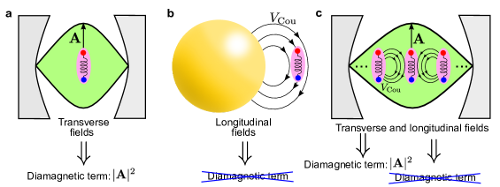
Figure 1: Schematics of the interaction between molecular excitations and cavity modes in the three systems considered in this work. a) A molecule placed inside a dielectric (Fabry-Pérot) cavity. The transverse field of the single cavity mode considered is described with the vector potential $\mathbf{A}$, which leads to the presence of the diamagnetic term $\propto|\mathbf{A}|^{2}$ in the cavity-QED Hamiltonian that describes this system. b) A molecule close to a metallic nanosphere and coupled to a single plasmonic mode. Within the quasistatic approximation, the molecule only interacts with the longitudinal fields of the nanosphere, via the Coulomb potential $V_{\text{Cou}}$. Since the vector potential $\mathbf{A}$ is not considered, the diamagnetic term is absent in the corresponding cavity-QED description. c) An ensemble of molecules placed inside a Fabry-Pérot cavity. In this system, each molecule interacts with the transverse cavity modes indicated by the vector potential $\mathbf{A}$ and with the longitudinal fields associated with the Coulomb potential $V_{\text{Cou}}$ induced by the other molecules. Whereas the interaction with cavity modes requires a diamagnetic term in the cavity-QED description, the coupling with other molecules is described without this term.

In this context, many recent studies focus on the strong and ultrastrong coupling between many molecules and microcavities or nanoresonators presenting optical modes (for simplicity, we often focus on nanophotonic systems but the discussion is also valid for systems of micrometer dimensions, except when stated otherwise). Introducing many molecules in a cavity increases the coupling strength substantially and to reach the strong and ultrastrong coupling regimes more easily in experiments. Under these circumstances, linear phenomena dominate and the optical response of the system is usually described with fully classical models based on coupled harmonic oscillators [32, 31, 33]. These classical coupled harmonic oscillator models have successfully described the avoided crossing of the hybrid modes [34], Fano resonances [35], stimulated Raman [36] and electromagnetic induced transparency [37, 38, 39]. Further, they are used to fit experimental data and to extract the coupling strength $g$, the frequencies of the hybrid modes and the fraction of light and matter corresponding to each mode [40, 41]. However, it is often not clear the exact physical magnitude that each oscillator represents, which can make it difficult to determine the value of a given observable in an experiment. Further, in a similar way as we have described the possibility to use two cavity-QED Hamiltonians to model light-matter coupling with or without diamagnetic term, different classical models have been used to analyze the strong and ultrastrong coupling regimes. These classical models are almost equivalent in the strong coupling but not in the ultrastrong coupling regime, leading e.g. to different frequencies of the hybrid modes and of the corresponding mode splitting. However, the choice of the model and its connection with the cavity-QED description is often not clearly justified [33, 43, 42]. Therefore, it can be useful to analyze in detail the relation between these classical models with the cavity-QED formalism, in order to understand better how to use and interpret the classical harmonic oscillator models and how each classical oscillator is related with physical magnitudes of the system. In this analysis, it is again critical to consider if the matter excitations couple with either the transverse electromagnetic fields (e.g. in conventional dielectric cavities) or the longitudinal fields characteristic of Coulomb coupling with plasmonic cavities.

In this work, we present a pedagogical overview of the different classical models of coupled harmonic oscillators that can be used to describe ultrastrong coupling in nanophotonics, and their connection with the equivalent cavity-QED description. We establish that the main light-matter coupling mechanism, i.e. either the coupling occurs via transverse electromagnetic fields or via Coulomb interactions, is the key to determine the right model of the system. In Sec. 2, we present in detail the two main classical coupled harmonic oscillator models under consideration and show that they lead to different dispersions of the hybrid modes as a function of the frequency of the cavity mode (other possible models are discussed in the Supplementary Information). In Sec. 3, we show that each classical model has a counterpart cavity-QED bosonic Hamiltonian that results in identical eigenfrequencies. In Sec. 4, we show that the connection between the amplitudes of the classical harmonic oscillators and the expectation values of quantum operators allows us to determine how to calculate physical observables within the classical description, such as the electric field of the cavity mode or the induced dipole moment of the matter excitation. With this aim, we consider in this section the three specific examples shown in Fig. 1. Specifically, we first discuss the application of coupled harmonic oscillator models in systems with transverse (molecule in a dielectric cavity, Sec. 4.1) and longitudinal (molecule coupled to a metallic nanoparticle via Coulomb interactions, Sec. 4.2) fields. We then consider a system or large relevance in studies of strong and ultrastrong coupling, which consists in an ensemble of molecules inside a Fabry-Pérot cavity [43, 44] and where both components of the electromagnetic fields (transverse and longitudinal) need to be considered (Sec. 4.3). Last, in Sec. 5, we present the main conclusions of this work.

2 Classical models of coupled harmonic oscillators in nanophotonics

In classical models of light-matter interaction based on coupled harmonic oscillators, one oscillator represents the degrees of freedom of the matter excitation, whose physical origin can be electronic or vibrational, for instance. The electromagnetic mode that couples with these matter excitations is modelled with another oscillator, and can correspond to a resonance of different types of optical resonators, such as Fabry-Pérot cavities, metallic planar layers supporting surface plasmon polaritons, nanocavities supporting localized plasmon polaritons, photonic crystals…

The interchange of energy between the matter and light degrees of freedom can be described by making an analogy with the widely-used spring mass model, as it is schematically shown in Fig. 2a. This model is able to capture the dynamics of strongly-coupled light-matter systems, such as Rabi oscillations [31]. In this approach, the cavity mode is replaced by a mass $m_{\text{cav}}$ attached to a spring with spring constant $k_{\text{cav}}$, while the matter excitation is modelled in the same way with a mass $m_{\text{mat}}$ and spring constant $k_{\text{mat}}$. These two masses are coupled with each other by a spring of spring constant $k_{\scriptscriptstyle{\text{SpC}}}$. The equations of motion for the displacements $X_{\text{cav}}$ and $X_{\text{mat}}$ of the oscillators from the equilibrium positions are

$$m_{\text{cav}}\ddot{X}_{\text{cav}}+k_{\text{cav}}X_{\text{cav}}+k_{\scriptscriptstyle{\text{SpC}}}(X_{\text{cav}}-X_{\text{mat}})=0,$$ (1a)

$$m_{\text{mat}}\ddot{X}_{\text{mat}}+k_{\text{mat}}X_{\text{mat}}-k_{\scriptscriptstyle{\text{SpC}}}(X_{\text{cav}}-X_{\text{mat}})=0.$$ (1b)

As will be analyzed in detail below, the displacements of the oscillators can in principle refer to different magnitudes of the nanophotonic system that oscillate during the Rabi oscillations. For instance, $X_{\text{mat}}$ can be related to the charges inside the matter structure, and $X_{\text{cav}}$ to the transverse electromagnetic fields of a dielectric cavity mode or to moving electrons inside a plasmonic nanocavity. Similarly, $m_{\text{cav}}$ and $m_{\text{mat}}$ can be seen as effective parameters whose meaning depends on the system and, at this stage, are not well defined. By defining the frequency of the cavity $\omega_{\text{cav}}=\sqrt{\frac{k_{\text{cav}}+k_{\scriptscriptstyle{\text{SpC}}}}{m_{\text{cav}}}}$, the frequency of the matter excitation $\omega_{\text{mat}}=\sqrt{\frac{k_{\text{mat}}+k_{\scriptscriptstyle{\text{SpC}}}}{m_{\text{mat}}}}$ and the coupling strength $g_{\scriptscriptstyle{\text{SpC}}}=\frac{k_{\text{SpC}}}{2\sqrt{m_{\text{cav}}m_{\text{mat}}}\sqrt{\omega_{\text{cav}}\omega_{\text{mat}}}}$, Eq. (1) can be rewritten as

$$\ddot{x}_{\text{cav}}+\omega_{\text{cav}}^{2}x_{\text{cav}}+2g_{\scriptscriptstyle{\text{SpC}}}\sqrt{\omega_{\text{cav}}\omega_{\text{mat}}}x_{\text{mat}}=0,$$ (2a)

$$\ddot{x}_{\text{mat}}+\omega_{\text{mat}}^{2}x_{\text{mat}}+2g_{\scriptscriptstyle{\text{SpC}}}\sqrt{\omega_{\text{cav}}\omega_{\text{mat}}}x_{\text{cav}}=0,$$ (2b)

where we have used the renormalized displacements $x_{\text{cav}}=\sqrt{m_{\text{cav}}}X_{\text{cav}}$ and $x_{\text{mat}}=\sqrt{m_{\text{mat}}}X_{\text{mat}}$. This transformation allows us to write the equations in a simpler way without indicating the masses of the oscillators $m_{\text{cav}}$ and $m_{\text{mat}}$ explicitly, and leaves the eigenfrequencies of the system invariant. We discuss in Sec. 4 how to connect $x_{\text{cav}}$ and $x_{\text{mat}}$ with the parameters governing specific systems. Further, we have not included losses (friction terms proportional to the time derivatives $\dot{x}_{\text{cav}}$ and $\dot{x}_{\text{mat}}$) in these equations in order to facilitate the comparison with Hermitian Hamiltonians of cavity-QED models. Neglecting losses is usually an excellent approximation for the calculation of the eigenfrequencies and eigenvectors of the system in the ultrastrong coupling regime, where the coupling strength can be much larger than the losses of the system. The eigenmodes of this model are obtained by writing Eq. (2b) in the frequency domain and diagonalizing the matrix associated with the resulting equations, which leads to the eigenfrequencies

$$\omega_{\pm,\scriptscriptstyle{\text{SpC}}}=\frac{1}{\sqrt{2}}\sqrt{\omega_{\text{cav}}^{2}+\omega_{\text{mat}}^{2}\pm\sqrt{(\omega_{\text{cav}}^{2}-\omega_{\text{mat}}^{2})^{2}+16g_{\scriptscriptstyle{\text{SpC}}}^{2}\omega_{\text{cav}}\omega_{\text{mat}}}}.$$ (3)

This simple coupled harmonic oscillator model has been used to extract the coupling strength $g_{\scriptscriptstyle{\text{SpC}}}$ by fitting the spectra of the hybrid modes obtained from experimental data or from simulations [16, 45, 17, 46, 47, 48, 49]. We refer to this model as the Spring Coupling (SpC) model, as it assumes that the coupling is mathematically equivalent to a spring attached to two masses. We emphasize that the SpC model is defined as the coupled harmonic oscillator model that satisfies two important properties as indicated in Eq. (2b): i) the coupling terms (third term in the left handsides) are proportional to the amplitudes $x_{\text{cav}}$ and $x_{\text{mat}}$; and ii) the frequencies that appear in the second term in the left handsides are the bare frequencies $\omega_{\text{cav}}$ and $\omega_{\text{mat}}$ corresponding to the uncoupled oscillators (without considering any modification in these frequencies as done in Sec. S2 in the SI).

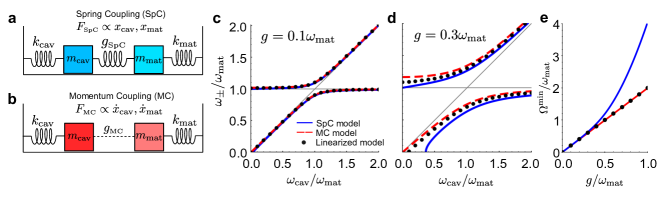
Figure 2: Comparison of the Spring Coupling (SpC), Momentum Coupling (MC) and linearized models. a) Schematics of the SpC model in analogy to an oscillator model in classical mechanics. The coupling mechanism of strength $g_{\scriptscriptstyle{\text{SpC}}}$ is analogous to a force $F_{\scriptscriptstyle{\text{SpC}}}$ exerted by a spring and that is proportional to the oscillator displacements $x_{\text{cav}}$ and $x_{\text{mat}}$. b) Schematics of the MC model. The coupling mechanism of strength $g_{\scriptscriptstyle{\text{MC}}}$ is analogous to a force $F_{\scriptscriptstyle{\text{MC}}}$ proportional to the time derivatives of the oscillator displacements $\dot{x}_{\text{cav}}$ and $\dot{x}_{\text{mat}}$. c) Eigenfrequencies $\omega_{\pm}$ as a function of the cavity frequency $\omega_{\text{cav}}$, obtained from the SpC model (blue solid line, corresponding to Eq. (3)), MC model (red dashed line, Eq. (6)) and the approximate linearized model (black dots, Eq. (8)), for coupling strength $g=0.1\,\omega_{\text{mat}}$. The thin gray lines correspond to the bare cavity frequency $\omega_{\text{cav}}$ and the bare frequency of the matter excitation, $\omega_{\text{mat}}$. d) Same as panel (c), for coupling strength $g=0.3\,\omega_{\text{mat}}$. e) Minimum splitting between the hybrid modes $\Omega^{\text{min}}=\omega_{+}-\omega_{-}$, as a function of the coupling strength $g$ for the SpC model (blue solid line), the MC model (red solid line) and the linearized model (black dots). All frequencies in panels (c-e) are normalized with respect to the fixed frequency of the matter excitation $\omega_{\text{mat}}$.

On the other hand, a different classical coupled harmonic oscillator model is also used [51, 50, 52, 53]:

$$\ddot{x}_{\text{cav}}+\omega_{\text{cav}}^{2}x_{\text{cav}}-2g_{\scriptscriptstyle{\text{MC}}}\dot{x}_{\text{mat}}=0,$$ (4a)

$$\ddot{x}_{\text{mat}}+\omega_{\text{mat}}^{2}x_{\text{mat}}+2g_{\scriptscriptstyle{\text{MC}}}\dot{x}_{\text{cav}}=0.$$ (4b)

These equations are very similar to Eq. (2b), but in this case the coupling terms are proportional to the time derivatives of the displacements $\dot{x}_{\text{cav}}$ and $\dot{x}_{\text{mat}}$ (i.e. to the velocities of the oscillators, in the analogy with the coupled masses). Equivalently, the coupling terms are proportional to the frequency $\omega$ in the frequency domain [42]:

$$(\omega_{\text{cav}}^{2}-\omega^{2})x_{\text{cav}}+2i\omega g_{\scriptscriptstyle{\text{MC}}}x_{\text{mat}}=0,$$ (5a)

$$(\omega_{\text{mat}}^{2}-\omega^{2})x_{\text{mat}}-2i\omega g_{\scriptscriptstyle{\text{MC}}}x_{\text{cav}}=0.$$ (5b)

Since in these equations the coupling term scales with the velocities of the oscillators, and hence with their linear momenta, we call this model the Momentum Coupling (MC) model (Fig. 2b). Similarly to the case of the SpC model, we emphasize that the frequencies in the MC model (appearing in the second term in the left handsides in Eq. (4b)) are the bare frequencies $\omega_{\text{cav}}$ and $\omega_{\text{mat}}$, as modifying these frequencies is equivalent to a change in the coupling term (see Sec. S2 in the SI) and thus it would correspond to a different type of model. The frequencies of the hybrid modes according to the MC model are

$$\omega_{\pm,\scriptscriptstyle{\text{MC}}}=\frac{1}{\sqrt{2}}\sqrt{\omega_{\text{cav}}^{2}+\omega_{\text{mat}}^{2}+4g_{\scriptscriptstyle{\text{MC}}}^{2}\pm\sqrt{(\omega_{\text{cav}}^{2}+\omega_{\text{mat}}^{2}+4g_{\scriptscriptstyle{\text{MC}}}^{2})^{2}-4\omega_{\text{cav}}^{2}\omega_{\text{mat}}^{2}}}.$$ (6)

At moderate coupling strengths $g$, corresponding to a system in the strong but not in the ultrastrong coupling regime, the frequencies of the hybrid modes are very similar for the two models. In this regime, by considering that the eigenfrequencies $\omega_{\pm}$ do not differ too strongly from the bare frequencies $\omega_{\alpha}$ ($\alpha$ = ’cav’ or $\alpha$ = ’mat’), we can make the approximation $\omega_{\alpha}+\omega\approx 2\omega$ to solve the equations for $\omega_{\pm}$. The frequency-domain equations of both the SpC and MC models become linear in $\omega$:

$$(\omega_{\text{cav}}-\omega)x_{\text{cav}}+g_{\scriptscriptstyle{\text{lin}}}x_{\text{mat}}=0\\$$ (7a)

$$(\omega_{\text{mat}}-\omega)x_{\text{mat}}+g_{\scriptscriptstyle{\text{lin}}}^{*}x_{\text{cav}}=0,$$ (7b)

with $g_{\scriptscriptstyle{\text{lin}}}=g_{\scriptscriptstyle{\text{SpC}}}$ (SpC model) or $g_{\scriptscriptstyle{\text{lin}}}=ig_{\scriptscriptstyle{\text{MC}}}$ (MC model). The resulting eigenfrequencies are in both cases

$$\omega_{\pm,\text{lin}}=\frac{\omega_{\text{cav}}+\omega_{\text{mat}}\pm\sqrt{(\omega_{\text{cav}}-\omega_{\text{mat}})^{2}+4|g_{\scriptscriptstyle{\text{lin}}}|^{2}}}{2}.$$ (8)

The validity of these linearized equations for $g=0.1\omega_{\text{mat}}$ (conventionally defined as the onset of the ultrastrong coupling regime) is analyzed in Fig. 2c, where we compare the eigenfrequencies of the SpC model (blue solid line), the MC model (red dashed line) and the linearized model (black dots). These eigenfrequencies are given by equations (3), (6) and (8), respectively, and plotted as a function of the cavity frequency $\omega_{\text{cav}}$ (all values in Fig. 2 are given as the ratio with the frequency $\omega_{\text{mat}}$, which remains fixed in all the panels of this figure). We find that the three curves follow a nearly identical dependence on the cavity frequency $\omega_{\text{cav}}$, and the agreement is even better for $g<0.1\,\omega_{\text{mat}}$. Thus, for systems not in the ultrastrong coupling regime, the three models can often be used equally with very small implications to the results.

In contrast, for even larger coupling strengths, corresponding to a system well into the ultrastrong coupling regime, the choice of the model is crucial. The differences between the three models are illustrated in Fig. 2d for coupling strength $g=0.3\,\omega_{\text{mat}}$. In this case, the three models predict significantly different eigenfrequencies of the coupled system. The difference is smaller for large cavity frequencies, $\omega_{\text{cav}}\gg\omega_{\text{mat}}$, because the oscillators become uncoupled and the eigenfrequencies approach the bare frequencies $\omega_{\text{cav}}$ and $\omega_{\text{mat}}$ in all models. However, even for a relatively large $\frac{\omega_{\text{cav}}}{\omega_{\text{mat}}}=1.5$, the difference between the values of $\omega_{\pm}$ according to the different models is around 10$\%$.

Further, comparing the three models in resonant conditions at zero detuning, $\omega_{\text{cav}}=\omega_{\text{mat}}$, the splitting $\Omega=\omega_{+}-\omega_{-}$ between the two eigenmodes is equal to twice the coupling strength in the linearized and in the MC model, i.e., $\Omega=2g$. This is the minimum splitting in these two models [54, 55]. On the other hand, in the SpC model the relation between $\Omega$ and the coupling strength for zero detuning is different:

$$\Omega_{\scriptscriptstyle{\text{SpC}}}=\omega_{+,\scriptscriptstyle{\text{SpC}}}-\omega_{-,\scriptscriptstyle{\text{SpC}}}=\omega_{\text{mat}}\left(\sqrt{1+\frac{2g_{\scriptscriptstyle{\text{SpC}}}}{\omega_{\text{mat}}}}-\sqrt{1-\frac{2g_{\scriptscriptstyle{\text{SpC}}}}{\omega_{\text{mat}}}}\right).$$ (9)

We find $\Omega_{\scriptscriptstyle{\text{SpC}}}=2.11g_{\scriptscriptstyle{\text{SpC}}}$ for the values used in Fig. 2d. Further, according to this model the minimum splitting between the branches does not happen at zero detuning, but at cavity frequencies larger than the matter excitation frequencies. To further emphasize the difference in the splitting between the models, we plot in Fig. 2e the minimum splitting $\Omega^{\text{min}}$ for the SpC model (blue solid line) as a function of the coupling strength, as compared to the $\Omega^{\text{min}}=2g$ linear relationship of the MC (red solid line) and the linearized model (black dots). For couplings too small to reach the ultrastrong coupling regime $\left(\frac{g}{\omega_{\text{mat}}}\lesssim 0.1\right)$, the splitting of the three models follows the same linear tendency. However, for larger values of $g$, within the ultrastrong coupling regime, the minimum splitting according to the SpC model deviates strongly from linearity, and close to the so-called deep strong coupling regime $\left(\frac{g}{\omega_{\text{mat}}}\approx 1\right)$, $\Omega^{\text{min}}_{\scriptscriptstyle{\text{SpC}}}$ is approximately the double than for the other two models. Last, Fig. 2d shows that a striking difference appears for small cavity frequencies, $\omega_{\text{cav}}\ll\omega_{\text{mat}}$. According to the MC model, for decreasing $\omega_{\text{cav}}$ the lower mode frequency $\omega_{-,\scriptscriptstyle{\text{MC}}}$ tends towards $\omega_{\text{cav}}$, but the upper branch approaches the limit $\omega_{+,\scriptscriptstyle{\text{MC}}}=\sqrt{\omega_{\text{mat}}^{2}+4g_{\scriptscriptstyle{\text{MC}}}^{2}}$ instead of the bare matter frequency, and thus this hybrid mode is affected by the coupling even in this highly detuned situation.

The behavior of $\omega_{-}$ and $\omega_{+}$ in the asymptotic limits of $\omega_{\text{cav}}$ has an interesting consequence on the range of energies where hybrid modes can exist according to each model. The dispersion of the MC model shows two hybrid modes for all values of the detuning and indicates that there is a band between $\omega_{\text{mat}}$ and $\sqrt{\omega_{\text{mat}}^{2}+4g_{\scriptscriptstyle{\text{MC}}}^{2}}$ with no modes available (as can be appreciated from the limits of the eigenfrequencies for $\omega_{\text{cav}}\rightarrow 0$ and $\omega_{\text{cav}}\rightarrow\infty$). For the SpC model, the upper mode approaches the bare frequency $\omega_{\text{mat}}$ for vanishing $\omega_{\text{cav}}$, but the lower mode ceases to exist ($\omega_{-,\scriptscriptstyle{\text{SpC}}}$ becomes imaginary) under the condition $\frac{\omega_{\text{cav}}}{\omega_{\text{mat}}}<\left(\frac{2g_{\scriptscriptstyle{\text{SpC}}}}{\omega_{\text{mat}}}\right)^{2}$. Further, by considering the total dispersion of the SpC model, we emphasize that we obtain hybrid modes at any frequency $\omega_{\pm,\scriptscriptstyle{\text{SpC}}}$ by tuning the bare frequencies $\omega_{\text{cav}}$ and $\omega_{\text{mat}}$, and thus there is no forbidden band as opposed to the MC model. Last, the dispersion of the linearized model lies between the dispersions of the other two models. In this case, there is a band of forbidden modes of spectral width half the value given by the MC model, and the lower mode disappears as in the SpC model but under a different inequality, because $\omega_{-,\text{lin}}$ becomes negative for frequencies $\frac{\omega_{\text{cav}}}{\omega_{\text{mat}}}<\left(\frac{g_{\scriptscriptstyle{\text{lin}}}}{\omega_{\text{mat}}}\right)^{2}$. In Sec. 4, we connect the finding of these bands with the Reststrahlen band of polar materials, and show that we can only reproduce the experimental dispersion with the correct width of the Reststrahlen band by using the MC model.

The analysis of Fig. 2d thus emphasizes that the three classical models considered can lead to distinctly different predictions of the eigenfrequencies of light-matter coupled systems in the ultrastrong coupling regime. These differences imply that the coupling terms of the SpC and MC models are related to different types of interactions between light and matter, and that not all electromagnetic interactions are mathematically equivalent to two coupled mechanical springs (i.e. to the SpC model). In order to better understand the origins of the SpC and MC models and their relation with Coulomb interactions and with interactions based on transverse electromagnetic modes, we compare in the next section the classical equations with those obtained using a cavity-QED model. Further, this section has focused on the eigenfrequencies, which can be extracted directly from the equations of coupled harmonic oscillators without an exact knowledge of what the displacements $x_{\text{cav}}$ and $x_{\text{mat}}$ represent. However, a clear physical interpretation of these parameters often becomes necessary to evaluate magnitudes of interest such as the electric field at a given position. We discuss in Sec. 4 how $x_{\text{cav}}$ and $x_{\text{mat}}$ relate to relevant physical quantities for representative systems.

3 Comparison of classical and cavity QED models

3.1 Spring Coupling model

We next analyze the light-matter interaction using a cavity-QED framework. The cavity modes and the matter excitations are quantized using bosonic operators, so that we can directly compare the cavity-QED description with the classical models in Section 2. The use of bosonic operators is valid for the cavity modes, as well as for matter excitations such as vibrations or phonons associated to a potential with a harmonic dependence on the degrees of freedom. For matter excitations of fermionic nature or with highly anharmonic behavior, the response can become dominated by non-linear effects that go beyond this work. However, the correspondence with classical oscillators can still be valid for weak excitation, i.e. weakly-populated states, and for systems with many particles. Under this description based on bosonic operators, we can use a Hopfield-type Hamiltonian [56] of the form

$$\hat{H}_{1}=\hbar\omega_{\text{cav}}\left(\hat{a}^{\dagger}\hat{a}+\frac{1}{2}\right)+\hbar\omega_{\text{mat}}\left(\hat{b}^{\dagger}\hat{b}+\frac{1}{2}\right)+\hbar g_{\scriptscriptstyle{\text{QED}}}(\hat{a}+\hat{a}^{\dagger})(\hat{b}+\hat{b}^{\dagger})+\hbar D(\hat{a}+\hat{a}^{\dagger})^{2}.$$ (10)

In this Hamiltonian, the creation operator $\hat{a}^{\dagger}$ and the annihilation operator $\hat{a}$ act on the cavity mode, while the equivalent operators $\hat{b}^{\dagger}$ and $\hat{b}$ are associated to the matter excitation, obeying commutation rules $[\hat{a},\hat{a}^{\dagger}]=[\hat{b},\hat{b}^{\dagger}]=1$. The first two terms in the right handside indicate the energy of the uncoupled cavity modes and matter excitations. The third term describes the light-matter coupling, which is parametrized by the coupling strength $g_{\scriptscriptstyle{\text{QED}}}$, and where we include the anti-resonant terms $\hat{a}\hat{b}$ and $\hat{a}^{\dagger}\hat{b}^{\dagger}$ required to describe correctly the ultrastrong coupling regime. Last, we introduce the diamagnetic term, scaled by a parameter $D$ that is initially considered to have an arbitrary value and can be zero. This last term is included in many (but not all) studies of ultrastrong coupling and originates from the $|\mathbf{A}|^{2}$ term of the minimal coupling Hamiltonian, where $\mathbf{A}$ is the vector potential of the cavity mode in the Coulomb gauge ($\nabla\cdot\mathbf{A}=0$). Further, the diamagnetic term is negligible in the strong coupling regime and only becomes important under ultrastrong coupling.

From the Hopfield Hamiltonian, we can obtain the equations of motion of the displacements of the two quantum oscillators, which will allow for a direct comparison with the classical SpC and MC models. To obtain these equations, we connect the creation and annihilation operators from the Hamiltonian in Eq. (10) with the quantum displacement ($\hat{X}_{\text{cav}}$ and $\hat{X}_{\text{mat}}$) and momentum ($\hat{P}_{\text{cav}}$ and $\hat{P}_{\text{mat}}$) operators, associated to two harmonic oscillators with masses $m_{\text{cav}}$ and $m_{\text{mat}}$ (as indicated in Eq. (1)). According to the quantization rules of harmonic oscillators, we use the relations $\hat{X}_{\text{cav}}=\sqrt{\frac{\hbar}{2m_{\text{cav}}\omega_{\text{cav}}}}(\hat{a}+\hat{a}^{\dagger})$, $\hat{X}_{\text{mat}}=\sqrt{\frac{\hbar}{2m_{\text{mat}}\omega_{\text{mat}}}}(\hat{b}+\hat{b}^{\dagger})$, $\hat{P}_{\text{cav}}=-i\sqrt{\frac{\hbar m_{\text{cav}}\omega_{\text{cav}}}{2}}(\hat{a}-\hat{a}^{\dagger})$ and $\hat{P}_{\text{mat}}=-i\sqrt{\frac{\hbar m_{\text{mat}}\omega_{\text{mat}}}{2}}(\hat{b}-\hat{b}^{\dagger})$. The dynamics of these four new displacement and momentum operators $\hat{O}$ is calculated from the Heisenberg equations of motion, $\frac{d}{dt}\hat{O}=\frac{1}{i\hbar}[\hat{O},\hat{H}]$. We convert the four resulting first-order differential equations into two second-order equations by eliminating the momentum operators. In this conversion, we consider the renormalized position operators in equivalence to the classical variables used in Sec. 2, i.e. $\hat{x}_{\text{cav}}=\sqrt{m_{\text{cav}}}\hat{X}_{\text{cav}}$ and $\hat{x}_{\text{mat}}=\sqrt{m_{\text{mat}}}\hat{X}_{\text{mat}}$. We obtain the following equations of motion for the expectation values $\langle\hat{x}_{\text{cav}}\rangle$ and $\langle\hat{x}_{\text{mat}}\rangle$:

$$\langle\ddot{\hat{x}}_{\text{cav}}\rangle+(\omega_{\text{cav}}^{2}+4D\omega_{\text{cav}})\langle\hat{x}_{\text{cav}}\rangle+2g_{\scriptscriptstyle{\text{QED}}}\sqrt{\omega_{\text{cav}}\omega_{\text{mat}}}\langle\hat{x}_{\text{mat}}\rangle=0,$$ (11a)

$$\langle\ddot{\hat{x}}_{\text{mat}}\rangle+\omega_{\text{mat}}^{2}\langle\hat{x}_{\text{mat}}\rangle+2g_{\scriptscriptstyle{\text{QED}}}\sqrt{\omega_{\text{cav}}\omega_{\text{mat}}}\langle\hat{x}_{\text{cav}}\rangle=0.$$ (11b)

We observe that for $D=0$ (no diamagnetic term) we recover the equations of motion from Eq. (2b) that correspond to the classical SpC model. The comparison between Eq. (2b) and Eq. (11b) also confirms that the quantum expectation values $\langle\hat{x}_{\text{cav}}\rangle$ and $\langle\hat{x}_{\text{mat}}\rangle$ correspond to the classical displacements $x_{\text{cav}}$ and $x_{\text{mat}}$.

To conclude, we note that the solutions of both the classical Eq. (2b) and quantum Eq. (11b) correspond to the energy of the transitions between two eigenstates, and not to the eigenfrequencies themselves. This distinction is not necessary in classical descriptions that set the energy of the ground state to zero (or a fixed value). However, the cavity-QED model indicates a $g_{\scriptscriptstyle{\text{QED}}}$-dependent shift of the ground-state energy from zero, which is a fully quantum phenomenon. The information of this shift is lost when we take the expectation value of the operators $\langle\hat{x}_{\text{cav}}\rangle$ and $\langle\hat{x}_{\text{mat}}\rangle$ in Eq. (11b), but can be recovered by solving the Schrödinger equation with the Hamiltonian of Eq. (10).

3.2 Momentum Coupling model

In order to recover the equations of motion of the MC model, we start from the same Hopfield Hamiltonian $\hat{H}_{1}$ in Eq. (10) and perform a unitary transformation with the operator $\hat{U}=e^{-i\frac{\pi}{2}\hat{b}^{\dagger}\hat{b}}$, which does not change the eigenfrequencies. In the new reference frame, the Hopfield-type Hamiltonian $\hat{H}_{2}=\hat{U}\hat{H}_{1}\hat{U}^{\dagger}+i\hbar\frac{\partial\hat{U}}{\partial t}\hat{U}^{\dagger}$ reads

$$\hat{H}_{2}=\hbar\omega_{\text{cav}}\left(\hat{a}^{\dagger}\hat{a}+\frac{1}{2}\right)+\hbar\omega_{\text{mat}}\left(\hat{b}^{\dagger\prime}\hat{b}^{\prime}+\frac{1}{2}\right)+i\hbar g_{\scriptscriptstyle{\text{QED}}}(\hat{a}+\hat{a}^{\dagger})(\hat{b}^{\prime}-\hat{b}^{\dagger\prime})+\hbar D(\hat{a}+\hat{a}^{\dagger})^{2},$$ (12)

where the prime ^′ denotes that the matter operators are transformed ($\hat{b}\rightarrow i\hat{b}^{\prime}$ and $\hat{b}^{\dagger}\rightarrow-i\hat{b}^{\dagger\prime}$). In the representation of position and momentum operators, this transformation can be understood as a rotation in the phase space, so that the canonical variables transform as

$$\hat{X}_{\text{mat}} \rightarrow-\frac{\hat{P}_{\text{mat}}^{\prime}}{m_{\text{mat}}\omega_{\text{mat}}},$$ (13a)

$$\hat{P}_{\text{mat}} \rightarrow m_{\text{mat}}\omega_{\text{mat}}\hat{X}_{\text{mat}}^{\prime}.$$ (13b)

In this new reference frame, we can calculate the equations of motion for the expectation values of the renormalized position operators $\langle\hat{x}_{\text{cav}}\rangle=\sqrt{m_{\text{cav}}}\langle\hat{X}_{\text{cav}}\rangle$ and $\langle\hat{x}^{\prime}_{\text{mat}}\rangle=\sqrt{m_{\text{mat}}}\langle\hat{X}^{\prime}_{\text{mat}}\rangle$:

$$\langle\ddot{\hat{x}}_{\text{cav}}\rangle+\left(\omega_{\text{cav}}^{2}+4D\omega_{\text{cav}}-4g_{\scriptscriptstyle{\text{MC}}}^{2}\right)\langle\hat{x}_{\text{cav}}\rangle-2g_{\scriptscriptstyle{\text{MC}}}\langle\dot{\hat{x}}^{\prime}_{\text{mat}}\rangle=0,$$ (14a)

$$\langle\ddot{\hat{x}}_{\text{mat}}^{\prime}\rangle+\omega_{\text{mat}}^{2}\langle\hat{x}_{\text{mat}}^{\prime}\rangle+2g_{\scriptscriptstyle{\text{MC}}}\langle\dot{\hat{x}}_{\text{cav}}\rangle=0.$$ (14b)

We recover the equations of motion of the MC model (Eq. (4b)) if we set $D=\frac{g_{\scriptscriptstyle{\text{MC}}}^{2}}{\omega_{\text{cav}}}$, which shows that the MC model is the classical equivalent to the quantum Hamiltonian with diamagnetic term and the given value of $D$ (which is the value normally used in cavity QED [22]). As a small difference, the coupling strength in the classical MC model is not identical to the corresponding value in the cavity-QED description (for $D=\frac{g_{\scriptscriptstyle{\text{QED}}}^{2}}{\omega_{\text{mat}}}=\frac{g_{\scriptscriptstyle{\text{MC}}}^{2}}{\omega_{\text{cav}}}$), but they are related as $g_{\scriptscriptstyle{\text{MC}}}=\sqrt{\frac{\omega_{\text{cav}}}{\omega_{\text{mat}}}}g_{\scriptscriptstyle{\text{QED}}}$ (in contrast, $g_{\scriptscriptstyle{\text{SpC}}}=g_{\scriptscriptstyle{\text{QED}}}$ in the case of the SpC model and $D=0$). Thus, if the classical coupling strength is assumed to be independent of the bare frequencies $\omega_{\text{cav}}$ and $\omega_{\text{mat}}$ (as expected from previous work that found excellent agreement with simulations and experiment [53]), then $g_{\scriptscriptstyle{\text{QED}}}$ must be modified with $\omega_{\text{cav}}$ and $\omega_{\text{mat}}$ to maintain the consistency of the equations of motion and the eigenvalues of the MC model.

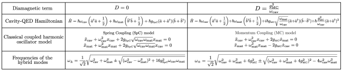
Table 1: Summary of the correspondences between the classical models and the cavity-QED description without diamagnetic term $D=0$ (second column) and with diamagnetic term of value $D=\frac{g_{\scriptscriptstyle{\text{MC}}}^{2}}{\omega_{\text{cav}}}$ (third column). The second row shows the two considered cavity-QED Hamiltonians. The third row indicates the equations of motion of the displacements $x_{\text{cav}}$ and $x_{\text{mat}}$ obtained with the classical SpC and MC harmonic oscillator models. The fourth row gives the frequencies of the two resulting hybrid modes, which are the same for the cavity-QED and classical models for the value of $D$ indicated in each column.

The connection between classical and quantum models is summarized in Table 1. The classical SpC and MC models result in the same eigenfrequencies as cavity-QED Hamiltonians without the diamagnetic term ($D=0$) and with $D=\frac{g_{\scriptscriptstyle{\text{MC}}}^{2}}{\omega_{\text{cav}}}$, respectively (we write in this table the quantum Hamiltonians in terms of the classical coupling strengths $g_{\scriptscriptstyle{\text{SpC}}}$ and $g_{\scriptscriptstyle{\text{MC}}}$ to show their equivalence appropriately). The correspondence between each classical model and these particular values of the parameter $D$ in the cavity-QED descriptions implies that the SpC model is well suited to describe the interaction of matter excitations with longitudinal fields, whereas the MC model is appropriate when transverse cavity modes are involved (see Fig. 1). Last, we have focused until here on the two classical models that are most used in the literature, but we discuss other alternatives in Sec. S2 of the SI. Specifically, we show that renormalizing the cavity frequency by the right amount in the model with coupling terms proportional to the time derivatives $\dot{x}_{\text{cav}}$ and $\dot{x}_{\text{mat}}$ leads to the same frequencies as for the SpC model without renormalization, or vice versa.

4 Physical observables obtained from classical models in configurations of interest

We now exploit the connection between classical and cavity-QED models to establish the relationship between the amplitudes $x_{\text{cav}}$ and $x_{\text{mat}}$ of the classical oscillators and physical observables of the light-matter coupled system (for example, the electric field inside the cavity). This relationship depends on the particular configuration, and it requires determining whether the SpC or the MC model describes better the system. Thus, to illustrate the procedure, we analyze the same three canonical examples in nanophotonics that we have already introduced (Fig. 1) and for which different cavity-QED Hamiltonians (with and without the diamagnetic term) are appropriate. In Sec. 4.1, we focus in the textbook case of a single molecule interacting with transverse electromagnetic modes of a resonant dielectric cavity (Fig. 1a). As the next example, we analyze in Sec. 4.2 a molecule close to a small metallic nanoparticle, where the coupling is governed by longitudinal Coulomb interactions (Fig. 1b). The last example (Sec. 4.3) consists on an ensemble of molecules (representing a bulk material) inside a Fabry-Pérot cavity, where the molecules couple with each other as well as with the transverse electromagnetic modes of the cavity (Fig. 1c).

4.1 A molecule interacting with a transverse mode of a dielectric cavity

We consider first the canonical quantum-optics system consisting in one dipole interacting with a single transverse mode of a resonant dielectric cavity. The dipole is associated to matter excitations, and it can represent an excitonic transition of a molecule or a transition between vibrational states, for example. Cavity-QED models of this system have successfully described phenomena such as the modification of the spontaneous emission rate of a molecule [57, 58], of the photon statistics of the emitted light [59, 60, 61] or of the coherence time of the quantum states [62].

To analyze how the physical observables associated with this system can be described classically, the whole derivation of the equations of motion of the classical variables is discussed in the SI (Sec. S1), but we summarize it in the following. We represent the molecule as two point charges with relative position $\mathbf{l}$ (forming a dipole), which experience Coulomb interactions determined by the potential $V_{\text{Cou}}(l)$ and we make the harmonic approximation of the potential with respect to the distance $l=|\mathbf{l}|$ between them, i.e. $V_{\text{Cou}}(l)=\frac{1}{2}m_{\text{red}}\omega_{\text{mat}}^{2}l^{2}$, where $m_{\text{red}}$ is the reduced mass of this two-body system. From this description, the dipole moment induced in the molecule is $\mathbf{d}=q\mathbf{l}$, where $q$ is the charge of the particles in the dipole. On the other hand, the cavity mode is characterized by the vector potential $\mathbf{A}$, which is the canonical position variable of the transverse electromagnetic fields [63]. This description does not include non-linear effects, which is valid for harmonic molecular vibrations and can also be useful for anharmonic vibrations or excitonic transitions under weak illumination, for example.

In Cavity QED, the standard approach to describe light-matter interactions in this system is to use the minimal-coupling Hamiltonian of the form $H_{\text{min-c}}=\frac{(\mathbf{p}-q\mathbf{A})^{2}}{2m_{\text{red}}}$, where $\mathbf{p}$ is the classical canonical momentum of the dipole. To prove that this classical Hamiltonian leads to the quantum Hamiltonian of Eq. (12) (with $D=\frac{g_{\scriptscriptstyle{\text{QED}}}^{2}}{\omega_{\text{mat}}}$), we use the following quantization relations [56, 63, 64]:

$$\hat{A}(\mathbf{r})=\sqrt{\frac{\hbar}{2\omega_{\text{cav}}\varepsilon_{0}V_{\text{eff}}}}\Xi(\mathbf{r})(\hat{a}+\hat{a}^{\dagger}),$$ (15)

$$\hat{\Pi}(\mathbf{r})=-i\sqrt{\frac{\hbar\omega_{\text{cav}}\varepsilon_{0}V_{\text{eff}}}{2}}\Xi(\mathbf{r})(\hat{a}-\hat{a}^{\dagger}),$$ (16)

$$\hat{d}=\sqrt{\frac{\hbar f_{\text{mat}}}{2\omega_{\text{mat}}}}(\hat{b}+\hat{b}^{\dagger}),$$ (17)

$$\hat{p}=-i\sqrt{\frac{\hbar\omega_{\text{mat}}}{2f_{\text{mat}}}}(\hat{b}-\hat{b}^{\dagger}),$$ (18)

where $\hat{\Pi}(\mathbf{r})$ is the canonical momentum associated to the vector potential $\hat{A}(\mathbf{r})$ (see Sec. S1 of the SI). The function $\Xi(\mathbf{r})$ accounts for the spatial distribution of the vector potential of the cavity mode and is normalized so that its maximum value is 1. Further, we have introduced the effective mode volume of the cavity field, $V_{\text{eff}}$, and the oscillator strength of the dipole $f_{\text{mat}}=\frac{q^{2}}{m_{\text{red}}}$. From the minimal-coupling Hamiltonian $H_{\text{min-c}}$, the light-matter interaction term is $H_{\text{int}}=\frac{-q\mathbf{p}\cdot\mathbf{A}}{m_{\text{red}}}$. By considering that the induced dipole moment and the vector potential form an angle $\theta$, and by using Eqs. (15) and (18), the interaction term of quantized Hamiltonian reads

$$\hat{H}_{\text{int}}=i\hbar\frac{1}{2}\sqrt{\frac{f_{\text{mat}}}{\varepsilon_{0}V_{\text{eff}}}}\sqrt{\frac{\omega_{\text{mat}}}{\omega_{\text{cav}}}}\Xi(\mathbf{r})\cos\theta(\hat{a}+\hat{a}^{\dagger})(\hat{b}-\hat{b}^{\dagger}).$$ (19)

Comparing this expression with the third term of the Hopfield Hamiltonian (Eq. (12)), we directly obtain that the coupling strength in the cavity-QED formalism is $g_{\scriptscriptstyle{\text{QED}}}=\frac{1}{2}\sqrt{\frac{f_{\text{mat}}}{\varepsilon_{0}V_{\text{eff}}}}\sqrt{\frac{\omega_{\text{mat}}}{\omega_{\text{cav}}}}\Xi(\mathbf{r})\cos\theta$. The maximum coupling strength $g_{\scriptscriptstyle{\text{QED}}}=\frac{1}{2}\sqrt{\frac{f_{\text{mat}}}{\varepsilon_{0}V_{\text{eff}}}}\sqrt{\frac{\omega_{\text{mat}}}{\omega_{\text{cav}}}}$, which we consider from now on, is achieved in the position of the maximum field $(\Xi(\mathbf{r})=1)$ and with optimal orientation ($\theta=0$). Further, the $\mathbf{A}^{2}$ term in the minimal-coupling Hamiltonian leads to a diamagnetic term (fourth term in the right handside of Eq. (12)) with $D=\frac{g_{\scriptscriptstyle{\text{QED}}}^{2}}{\omega_{\text{mat}}}$. Following the discussion of Sec. 3, the presence of the diamagnetic term in the cavity-QED Hamiltonian with this exact value of $D$ indicates that the classical equivalent model of this system is the MC model.

Next, we use the connection between the classical and cavity-QED approaches to illustrate how to obtain the value of physical observables from the classical oscillator amplitudes $x_{\text{cav}}$ and $x_{\text{mat}}$. The classical coupling strength $g_{\scriptscriptstyle{\text{MC}}}$ is directly obtained from the quantum value as $g_{\scriptscriptstyle{\text{MC}}}=\sqrt{\frac{\omega_{\text{cav}}}{\omega_{\text{mat}}}}g_{\scriptscriptstyle{\text{QED}}}=\frac{1}{2}\sqrt{\frac{f_{\text{mat}}}{\varepsilon_{0}V_{\text{eff}}}}$. Further, the quantum position operators ($\propto\hat{a}+\hat{a}^{\dagger}$ and $\propto\hat{b}+\hat{b}^{\dagger}$ for the cavity and dipole, respectively) and the classical amplitudes of the cavity $x_{\text{cav}}$ and of the molecular excitation $x_{\text{mat}}$ are related by the standard quantization relationship

$$x_{\text{cav}}=\langle\hat{x}_{\text{cav}}\rangle=\sqrt{\frac{\hbar}{2\omega_{\text{cav}}}}\langle\hat{a}+\hat{a}^{\dagger}\rangle,$$ (20a)

$$x_{\text{mat}}=\langle\hat{x}_{\text{mat}}\rangle=\sqrt{\frac{\hbar}{2\omega_{\text{mat}}}}\langle\hat{b}+\hat{b}^{\dagger}\rangle.$$ (20b)

By comparing Eq. (20a) with Eq. (15), we obtain that the cavity oscillator amplitude $x_{\text{cav}}$ in the MC model (Eq. (4b)) is given by $x_{\text{cav}}=\mathcal{A}\sqrt{\varepsilon_{0}V_{\text{eff}}}$, where $\mathcal{A}$ is the maximum amplitude of the classical vector potential (i.e. in the position where $\Xi(\mathbf{r})=1$). Therefore, the oscillator amplitude $x_{\text{cav}}$ can be used to calculate the spatial distribution of this potential as $A(\mathbf{r})=\mathcal{A}\Xi(\mathbf{r})=\frac{x_{\text{cav}}}{\sqrt{\varepsilon_{0}V_{\text{eff}}}}\Xi(\mathbf{r})$ ($A(\mathbf{r})=\langle\hat{A}(\mathbf{r})\rangle$ is the classical counterpart of the quantum operator of the vector potential). Equivalently, from Eqs. (20b) and (17), the amplitude of the oscillator corresponding to the matter excitation is directly connected with the induced classical dipole moment $d=|\mathbf{d}|$ as $x_{\text{mat}}=\frac{d}{\sqrt{f_{\text{mat}}}}$. These relations are schematically shown in Fig. 3a.

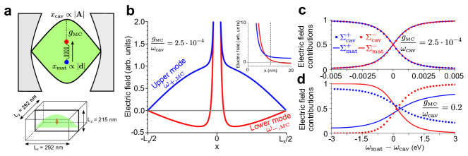
Figure 3: Interaction of a molecule with a transverse cavity mode within the classical MC model. a) Schematics of the system. The two oscillators are associated with the vector potential $\mathbf{A}$ of the cavity mode and the induced dipole moment $\mathbf{d}$ of the molecular excitation. The oscillators are coupled with each other with strength $g_{\scriptscriptstyle{\text{MC}}}$. The bottom sketch indicates the dimensions of the cavity that we analyze in the rest of the panels. The dipole is placed at the center of the cavity. The green shaded areas in the sketches represent the field distribution of the cavity mode. b) Spatial distribution of the electric field for the upper (blue) and the lower (red) hybrid modes at frequencies $\omega_{+,\scriptscriptstyle{\text{MC}}}$ and $\omega_{-,\scriptscriptstyle{\text{MC}}}$, respectively, for coupling strength $g_{\scriptscriptstyle{\text{MC}}}=2.5\cdot 10^{-4}\omega_{\text{cav}}$. The electric field is calculated along the axis of the cavity (along the $x$ direction in panel (a), with $x=y=z=0$ corresponding to the cavity center). The inset is a zoom of the region near the molecule. c) Contribution to the electric field from the cavity $\Sigma_{\text{cav}}^{\pm}$ (dots) and from the molecule $\Sigma_{\text{mat}}^{\pm}$ (solid lines), for the hybrid mode at frequency $\omega_{+,\scriptscriptstyle{\text{MC}}}$ (blue) and the hybrid mode at frequency $\omega_{-,\scriptscriptstyle{\text{MC}}}$ (red), as a function of the detuning $\omega_{\text{mat}}-\omega_{\text{cav}}$. The fields are evaluated at the position $(x,y,z)$ = (10.5 nm, 0, 0), i.e. at 10.5 nm distance from the center of the cavity where the molecule is situated (see sketch in (a) for directions), which corresponds to the position indicated by the dashed line in the inset of panel (b). The coupling strength is $g_{\scriptscriptstyle{\text{MC}}}=2.5\cdot 10^{-4}\omega_{\text{cav}}$. d) Same as in (c), for $g_{\scriptscriptstyle{\text{MC}}}=0.2\,\omega_{\text{cav}}$.

We are now finally in conditions to obtain the value of physical observables such as the electric field from the classical harmonic MC model. We first show how to obtain the spatial distribution of the electric fields corresponding to each hybrid mode. The transverse cavity mode field (given by $\mathbf{A}(\mathbf{r},t)$) must be added to the longitudinal near field induced by the dipole, which is obtained from the scalar Coulomb potential

$$V_{\text{Cou}}(\mathbf{r},t)=\frac{1}{4\pi\varepsilon_{0}}\frac{d(t)\mathbf{n_{d}}\cdot\mathbf{n_{r}}}{|\mathbf{r}|^{2}},$$ (21)

with the unit vectors $\mathbf{n_{d}}=\frac{\mathbf{d}}{|\mathbf{d}|}$ and $\mathbf{n_{r}}=\frac{\mathbf{r}}{|\mathbf{r}|}$. The total electric field is therefore given as

$$\mathbf{E}(\mathbf{r},t)=-\nabla V_{\text{Cou}}(\mathbf{r},t)-\frac{\partial\mathbf{A}(\mathbf{r},t)}{\partial t},$$

and the electric field at frequencies $\omega_{\pm,\scriptscriptstyle{\text{MC}}}$ of each hybrid mode (given by Eq. (6)) corresponds to

$$\mathbf{E}(\mathbf{r},\omega_{\pm,\scriptscriptstyle{\text{MC}}})= \frac{3(\mathbf{n_{d}}\cdot\mathbf{n_{r}})\mathbf{n_{r}}-\mathbf{n_{d}}}{4\pi\varepsilon_{0}r^{3}}d(\omega_{\pm,\scriptscriptstyle{\text{MC}}})+i\omega_{\pm,\scriptscriptstyle{\text{MC}}}A(\mathbf{r},\omega_{\pm,\scriptscriptstyle{\text{MC}}})\mathbf{n}_{\alpha}$$

$$= \underbrace{\frac{3(\mathbf{n_{d}}\cdot\mathbf{n_{r}})\mathbf{n_{r}}-\mathbf{n_{d}}}{4\pi\varepsilon_{0}r^{3}}\sqrt{f_{\text{mat}}}x_{\text{mat}}(\omega_{\pm,\scriptscriptstyle{\text{MC}}})}_{\mathbf{E}_{\text{mat}}(\mathbf{r},\omega_{\pm,\scriptscriptstyle{\text{MC}}})}+\underbrace{\frac{i\Xi(\mathbf{r})}{\sqrt{\varepsilon_{0}\mathcal{V}_{\text{eff}}}}\omega_{\pm,\scriptscriptstyle{\text{MC}}}x_{\text{cav}}(\omega_{\pm,\scriptscriptstyle{\text{MC}}})\mathbf{n}_{\alpha}}_{\mathbf{E}_{\text{cav}}(\mathbf{r},\omega_{\pm,\scriptscriptstyle{\text{MC}}})},$$ (22)

with $\mathbf{n_{A}}=\frac{\mathbf{A}(\mathbf{r})}{|\mathbf{A}(\mathbf{r})|}$. According to this equation, the oscillator amplitude of the cavity mode $x_{\text{cav}}$ gives directly the contribution of the cavity to the electric field, $\mathbf{E}_{\text{cav}}(\mathbf{r},\omega_{\pm,\scriptscriptstyle{\text{MC}}})$, whereas the oscillator amplitude $x_{\text{mat}}$ is related to the contribution of the matter excitation $\mathbf{E}_{\text{mat }}(\mathbf{r},\omega_{\pm,\scriptscriptstyle{\text{MC}}})$. Further, we use Eq. (5) to obtain the ratio between the amplitudes $x_{\text{cav}}$ and $x_{\text{mat}}$ of the classical harmonic oscillators:

$$\frac{x_{\text{cav}}(\omega_{\pm,\scriptscriptstyle{\text{MC}}})}{x_{\text{mat}}(\omega_{\pm,\scriptscriptstyle{\text{MC}}})}=\frac{-2i\omega_{\pm,\scriptscriptstyle{\text{MC}}}g_{\scriptscriptstyle{\text{MC}}}}{\omega_{\text{cav}}^{2}-\omega_{\pm,\scriptscriptstyle{\text{MC}}}^{2}}.$$ (23)

Inserting Eq. (23) into Eq. (22), we obtain the ratio between the electric field contribution of the cavity and of the matter excitation.

Equations (22) and (23) are the main result of this subsection and are valid to obtain the electric field at any position and for an arbitrary transverse mode with field distribution given by $\Xi(\mathbf{r})$. We consider for illustration the particular case of a molecule introduced in the center of a rectangular vacuum box enclosed in the three dimensions by perfect mirrors, as sketched in Fig. 3a. The cross section of the box is square, with size $L_{x}=L_{y}=$ 292 nm and its height is $L_{z}=$ 215 nm, which results in a fundamental lowest-order mode at frequency $\omega_{\text{cav}}$ = 3 eV and an effective volume $V_{\text{eff}}=4.483\cdot 10^{6}\text{ nm}^{3}$. This value of $V_{\text{eff}}$ is calculated from the general expression of dielectric structures [65]

$$V_{\text{eff}}=\frac{\int\varepsilon(\mathbf{r})|\Xi(\mathbf{r})|^{2}d\mathbf{r}}{\max[\varepsilon(\mathbf{r})|\Xi(\mathbf{r})|^{2}]},$$ (24)

where $\varepsilon(\mathbf{r})$ refers to the permittivity of the system at position $\mathbf{r}$, and in this particular case we consider $\varepsilon(\mathbf{r})=1$ inside the cavity. The molecular excitation is nearly resonant with the cavity, $\omega_{\text{mat}}\approx\omega_{\text{cav}}=$ 3 eV, but its exact frequency is changed to study the effects of the detuning. The transition dipole moment $\mu_{\text{mat}}=\sqrt{\frac{\hbar f_{\text{mat}}}{2\omega_{\text{mat}}}}$ (corresponding to the transition from the ground state to the first excited state) is parallel to the $z$ axis and is relatively strong, $\mu_{\text{mat}}$ = 15 Debye, achievable with nonacene, for example [66]. This value of the transition dipole moment implies that this molecule has an oscillator strength of $f_{\text{mat}}=\frac{(118.74e)^{2}}{m_{\text{p}}}$, where $e$ is the electron charge and $m_{\text{p}}$ the mass of the proton. By placing the molecule in the center of the cavity where the electric field of the mode is maximum, this choice of parameters leads to a coupling strength $g_{\scriptscriptstyle{\text{MC}}}\approx 2.5\cdot 10^{-4}\omega_{\text{cav}}$, far from the ultrastrong coupling regime (a larger value of $g_{\scriptscriptstyle{\text{MC}}}$ is considered at the end of this subsection).

We show in Fig. 3b the distribution of the $z$ component of the electric field inside this cavity for the upper hybrid mode $E_{z}(x,\omega_{+,\scriptscriptstyle{\text{MC}}})$ and for the lower hybrid mode $E_{z}(x,\omega_{-,\scriptscriptstyle{\text{MC}}})$, as obtained from Eq. (22). We plot the fields as a function of the position in the $x$ direction with respect to the location of the dipole at the center of the cavity. To highlight the differences between the contributions of the cavity and the dipole in the two modes, we choose a slight detuning of $\omega_{\text{cav}}-\omega_{\text{mat}}=1.5$ meV. Since the classical MC model does not give the absolute value of the eigenmode fields, we choose arbitrary units so that the contribution of the cavity mode to the electric field of the upper hybrid mode ($\mathbf{E}_{\text{cav}}(\mathbf{r},\omega_{+,\scriptscriptstyle{\text{MC}}})$ in Eq. (22)) has a maximum absolute value of 1, and this choice fixes all the other values according to Eq. (23). The field distribution shows a clear difference in the behavior of the two hybrid modes, where for the upper mode the dipole points in the same direction as the cavity field ($\frac{x_{\text{cav}}(\omega_{+,\scriptscriptstyle{\text{MC}}})}{x_{\text{mat}}(\omega_{+,\scriptscriptstyle{\text{MC}}})}>0$), but in the inverse direction for the lower mode ($\frac{x_{\text{cav}}(\omega_{-,\scriptscriptstyle{\text{MC}}})}{x_{\text{mat}}(\omega_{-,\scriptscriptstyle{\text{MC}}})}<0$). Further, at the chosen detuning, the relative contribution of the cavity to the fields is larger for the upper than the lower mode, as indicated by the values of the electric field far from the molecule at $\omega_{+,\scriptscriptstyle{\text{MC}}}$ and $\omega_{-,\scriptscriptstyle{\text{MC}}}$. In contrast, as shown in the inset, the relative contribution from the dipole to the field close to the molecule ($x=0$) is stronger for the lower mode. Figure 3b thus confirms that the classical harmonic oscillator model allows for the calculation of the relative contribution of cavity and matter for each mode, as desired.

In addition to the spatial distribution of the electric field of the two hybrid modes, Eqs. (22) and (23) also enable to plot the dependence of the field $\mathbf{E}(\mathbf{r},\omega_{\pm,\scriptscriptstyle{\text{MC}}})$ inside the same cavity on the detuning $\omega_{\text{mat}}-\omega_{\text{cav}}$. Figure 3c shows for each mode the contributions to this electric field of the cavity and the molecule, normalized with respect to the sum of both contributions, according to $\Sigma_{\text{cav}}^{\pm}=\frac{|\mathbf{E}_{\text{cav}}(\omega_{\pm,\scriptscriptstyle{\text{MC}}})|^{2}}{|\mathbf{E}_{\text{cav}}(\omega_{\pm,\scriptscriptstyle{\text{MC}}})|^{2}+|\mathbf{E}_{\text{mat}}(\omega_{\pm,\scriptscriptstyle{\text{MC}}})|^{2}}$ (dots) and $\Sigma_{\text{mat}}^{\pm}=\frac{|\mathbf{E}_{\text{mat}}(\omega_{\pm,\scriptscriptstyle{\text{MC}}})|^{2}}{|\mathbf{E}_{\text{cav}}(\omega_{\pm,\scriptscriptstyle{\text{MC}}})|^{2}+|\mathbf{E}_{\text{mat}}(\omega_{\pm,\scriptscriptstyle{\text{MC}}})|^{2}}$ (solid lines). These ratios play a similar role as the Hopfield coefficients from cavity QED. The blue (red) dots and solid lines correspond to the upper (lower) hybrid mode. We obtain $\mathbf{E}_{\text{cav}}(\omega_{\pm,\scriptscriptstyle{\text{MC}}})$ and $\mathbf{E}_{\text{mat}}(\omega_{\pm,\scriptscriptstyle{\text{MC}}})$ by replacing Eq. (23) into Eq. (22), for a fixed coupling strength $g_{\scriptscriptstyle{\text{MC}}}=2.5\cdot 10^{-4}\omega_{\text{cav}}$ and for a distance of 10.5 nm from the dipole in the $x$ direction. This position (indicated by the dashed line in the inset of Fig. 3b) is chosen because it is where the contributions of the matter and cavity have the same weight for the two hybrid modes at zero detuning for such small coupling strengths ($\Sigma_{\text{cav}}^{\pm}=\Sigma_{\text{mat}}^{\pm}\approx 0.5$, as shown in Fig. 3c). For detunings such that $\omega_{\text{cav}}>\omega_{\text{mat}}$ the field of the lower mode is predominantly given by the matter excitation ($\Sigma_{\text{mat}}^{-}>\Sigma_{\text{cav}}^{-}$ as indicated by the red dots and the red solid line), while for the upper mode the cavity contribution dominates ($\Sigma_{\text{cav}}^{+}>\Sigma_{\text{mat}}^{+}$, blue). Further, already at detunings as small as $\omega_{\text{cav}}-\omega_{\text{mat}}\gtrsim 15\text{ meV}=5\cdot 10^{-3}\omega_{\text{cav}}$, the modes are essentially uncoupled for this small coupling strength ($\Sigma_{\text{mat}}^{+}\ll\Sigma_{\text{cav}}^{+}$ and $\Sigma_{\text{mat}}^{-}\gg\Sigma_{\text{cav}}^{-}$).

The coupling strength that we have considered up to now in this subsection corresponds to the strong coupling regime (we have neglected losses), far from the ultrastrong coupling regime, so that the phenomena studied can also be explained with the classical linearized model. On the other hand, we consider again in Fig. 3d the contributions to the electric field $\Sigma_{\text{cav}}^{\pm}$ and $\Sigma_{\text{mat}}^{\pm}$ as a function of the detuning, but in this case for a considerably larger coupling strength $g_{\scriptscriptstyle{\text{MC}}}=0.2\omega_{\text{cav}}$. This value of $g_{\scriptscriptstyle{\text{MC}}}$ is not currently achievable with dielectric cavities at the single molecule level, but we choose it to illustrate the analysis of a ultrastrongly-coupled systems within the classical MC model. Further, such large $g_{\scriptscriptstyle{\text{MC}}}$ can be achieved in systems with many molecules, as discussed in Sec. 4.3. For zero detuning $\omega_{\text{cav}}=\omega_{\text{mat}}$, the contributions of the dipole and the cavity are no longer identical in the ultrastrong coupling regime, with $\Sigma_{\text{cav}}^{+}\approx 0.6$ and $\Sigma_{\text{mat}}^{+}\approx 0.4$ for the upper hybrid mode at frequency $\omega_{+,\scriptscriptstyle{\text{MC}}}$ (and the opposite for the lower hybrid mode). More strikingly, the results in Fig. 3d indicate a qualitatively very different tendency of the modes at large detunings as compared to strong coupling, especially in the case of the upper hybrid mode. In ultrastrong coupling, in the $\omega_{\text{mat}}\rightarrow 0$ limit ($\omega_{\text{mat}}-\omega_{\text{cav}}\rightarrow-3$ eV), this mode at frequency $\omega_{+,\scriptscriptstyle{\text{MC}}}$ (blue solid line and dots) has significant contributions from both the cavity and the matter ($\Sigma_{\text{cav}}^{+}\approx 0.9$ and $\Sigma_{\text{mat}}^{+}\approx 0.1$), and thus these two excitations do not decouple in this limit. This behavior is consistent with the discussion of the dispersion in Fig. 2d, where at large detunings the upper mode frequency does not reach the bare frequency $\omega_{\text{cav}}$ or $\omega_{\text{mat}}$. The SpC, as well as the linearized model (not shown), do not reproduce this behavior, because in the SpC model the modes become uncoupled ($\Sigma_{\text{cav}}^{+}\approx 1$ and $\Sigma_{\text{mat}}^{+}\approx 0$), while in the linearized model we obtain intermediate values between those corresponding to the SpC and MC models. In summary, we have shown in this section how to use the classical MC model to characterize the fields in a hybrid system composed by a molecule coupled to a transverse mode of a cavity. The methodology described enables to obtain equivalent results to the cavity-QED description (Hopfield Hamiltonian with diamagnetic term) by using an intuitive classical model of coupled harmonic oscillators.

4.2 A molecule interacting with the longitudinal field of a metallic nanoparticle

As an alternative system to analyze how to obtain physical observables in the strong and ultrastrong coupling regimes, we now consider a molecule placed close to a metallic nanoparticle. These nanoparticles are attractive in nanophotonics because they support localized surface plasmon modes characterized by very low effective volumes [67, 68, 69, 66, 17]. Since the coupling strength is inversely proportional to the square root of the effective mode volume, large coupling strengths can be obtained even when the nanoparticle interacts with a single molecule, as desired to reach the ultrastrong coupling regime.

In order to analyze the interaction of the nanoparticle with a molecular (bosonic) excitation of dipole moment $d_{\text{mat}}$, we consider that the size of the nanoparticle and the molecule-nanoparticle distance are much smaller than the light wavelength, and treat the system within the quasistatic approximation. Under this approximation, the temporal variation of the vector potential $\mathbf{A}$ in Eq. (4.1) is negligible and therefore the coupling between the nanoparticle and the molecule is governed by Coulomb interactions expressed by the scalar potential $V_{\text{Cou}}$. Therefore, the interactions governing this system are different from those analyzed in Sec. 4.1, because while in the previous subsection the electromagnetic fields coupled to the molecule are mainly transverse, in this system we consider longitudinal fields.

For simplicity, we consider small spherical particles of radius $R_{\text{cav}}$ that are composed by a Drude metal with plasma frequency $\omega_{\text{p}}$. These particles present a dipolar plasmonic resonance of Lorentzian lineshape at frequency $\omega_{\text{cav}}=\frac{\omega_{\text{p}}}{\sqrt{3}}$, oscillator strength $f_{\text{cav}}=4\pi\varepsilon_{0}R_{\text{cav}}^{3}\omega_{\text{cav}}^{2}$ and dipole moment $d_{\text{cav}}$ [70]. In this context, the molecule-nanoparticle coupling cannot be modelled with the minimal coupling Hamiltonian as in Sec. 4.1 and it is described instead with the interaction Hamiltonian [71]

$$\hat{H}_{\text{int2}}=-\hat{\mathbf{d}}_{\text{mat}}\cdot\hat{\mathbf{E}}_{\text{cav}}(\mathbf{r}_{\text{mat}}).$$ (25)

$\hat{\mathbf{E}}_{\text{cav}}$ is the electric field associated to the dipolar mode of the nanocavity, which in the quasistatic approximation is completely longitudinal and directly determined by the dipole moment as $\hat{\mathbf{E}}_{\text{cav}}(\mathbf{r})=\frac{3(\hat{\mathbf{d}}_{\text{cav}}\cdot\mathbf{n}_{\mathbf{r}\text{cav}})\mathbf{n}_{\mathbf{r}\text{cav}}-\hat{\mathbf{d}}_{\text{cav}}}{4\pi\varepsilon_{0}|\mathbf{r}_{\text{cav}}-\mathbf{r}|^{3}}$ outside the spherical nanoparticle ($|\mathbf{r}-\mathbf{r}_{\text{cav}}|>R_{\text{cav}}$), where $\mathbf{r}_{\text{cav}}$ is the center of the nanoparticle and we define the unit vector $\mathbf{n}_{\mathbf{r}\text{cav}}=\frac{\mathbf{r}-\mathbf{r}_{\text{cav}}}{|\mathbf{r}-\mathbf{r}_{\text{cav}}|}$. We insert the quantized expressions of the dipole moments $\hat{d}_{\text{cav}}$ and $\hat{d}_{\text{mat}}$ of Eq. (17) into the Hamiltonian in Eq. (25) and obtain

$$\hat{H}_{\text{int2}}=\hbar g_{\scriptscriptstyle{\text{SpC}}}(\hat{a}+\hat{a}^{\dagger})(\hat{b}+\hat{b}^{\dagger}),$$ (26)

with coupling strength

$$g_{\scriptscriptstyle{\text{SpC}}}=\frac{1}{2}\frac{\sqrt{f_{\text{cav}}}\sqrt{f_{\text{mat}}}}{4\pi\varepsilon_{0}|\mathbf{r}_{\text{cav}}-\mathbf{r}_{\text{mat}}|^{3}\sqrt{\omega_{\text{cav}}\omega_{\text{mat}}}}[\mathbf{n}_{\mathbf{d}\text{cav}}\cdot\mathbf{n}_{\mathbf{d}\text{mat}}-3(\mathbf{n}_{\mathbf{d}\text{cav}}\cdot\mathbf{n}_{\mathbf{r}\text{rel}})(\mathbf{n}_{\mathbf{d}\text{mat}}\cdot\mathbf{n}_{\mathbf{r}\text{rel}})],$$ (27)

where we have defined the unit vectors as $\mathbf{n}_{\mathbf{d}\text{cav}}=\frac{\mathbf{d}_{\text{cav}}}{|\mathbf{d}_{\text{cav}}|}$, $\mathbf{n}_{\mathbf{d}\text{mat}}=\frac{\mathbf{d}_{\text{mat}}}{|\mathbf{d}_{\text{mat}}|}$ and $\mathbf{n}_{\mathbf{r}\text{rel}}=\frac{\mathbf{r}_{\text{cav}}-\mathbf{r}_{\text{mat}}}{|\mathbf{r}_{\text{cav}}-\mathbf{r}_{\text{mat}}|}$. The total Hamiltonian is thus the sum of $\hat{H}_{\text{int2}}$ and the terms related to the energy of the uncoupled plasmon and molecular excitation, corresponding to the Hopfield Hamiltonian of Eq. (10) without the diamagnetic term $(D=0)$. Thus, as justified in Sec. 3.1, the corresponding classical model is the SpC model, with the equations of motion in Eq. (2b).

The representation of the plasmon-molecule system with the SpC model is schematically shown in Fig. 4a. To obtain the observables in this system, we need to establish the equivalence of the oscillator amplitudes $x_{\text{cav}}$ and $x_{\text{mat}}$ with the dipole moments of the cavity and the molecular (or matter) excitation. This equivalence can be obtained from Eqs. (17) and (20b), as discussed in Sec. 4.1, and it follows $x_{\text{cav}}=\frac{d_{\text{cav}}}{\sqrt{f_{\text{cav}}}}$ and $x_{\text{mat}}=\frac{d_{\text{mat}}}{\sqrt{f_{\text{mat}}}}$. Further, this treatment is generalizable to other dipole-dipole interactions beyond the coupling of a molecule with a plasmon (molecule-molecule interactions are considered in the next section).

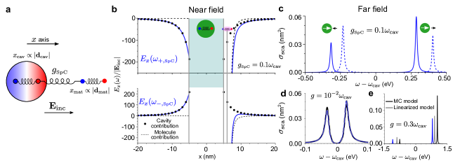
Figure 4: Modelling of the coupling between a molecule and a spherical nanoparticle (a nanocavity) within the classical SpC model. a) Schematics of the system. The molecular excitation (of induced dipole moment $\mathbf{d}_{\text{mat}}$) and the dipolar mode of the plasmonic nanocavity (of induced dipole moment $\mathbf{d}_{\text{cav}}$) are described as two harmonic oscillators (with oscillation amplitudes $x_{\text{mat}}$ and $x_{\text{cav}}$) that are coupled with strength $g_{\scriptscriptstyle{\text{SpC}}}$. The system is excited by a laser with electric field $\mathbf{E}_{\text{inc}}$. The radius of the spherical nanocavity is 5 nm and the dipole is placed at 1 nm distance from the surface of the nanoparticle along the $x$ axis (the center of the nanoparticle corresponds to $x=y=z=0$). $\mathbf{d}_{\text{cav}}$, $\mathbf{d}_{\text{mat}}$ and $\mathbf{E}_{\text{inc}}$ are polarized along $x$. b) Electric field distribution along the $x$ axis ($y=z=0$) when the system is excited at the frequency of the upper hybrid mode $\omega_{+,\scriptscriptstyle{\text{SpC}}}$ (top panel) and of the lower hybrid mode $\omega_{-,\scriptscriptstyle{\text{SpC}}}$ (bottom panel). The fields are evaluated only outside the nanocavity, with the positions inside highlighted by the green-shaded area. The position of the molecule is indicated by the vertical gray line. We evaluate the fields for coupling strength $g_{\scriptscriptstyle{\text{SpC}}}=0.1\,\omega_{\text{cav}}$ and the following parameters: $f_{\text{mat}}=(118.74e)^{2}/m_{\text{p}}$, $f_{\text{cav}}=(4345e)^{2}/m_{\text{p}}$, $F_{\text{cav}}=\sqrt{f_{\text{cav}}}|\mathbf{E}_{\text{inc}}|$, $F_{\text{mat}}=\sqrt{f_{\text{mat}}}|\mathbf{E}_{\text{inc}}|$, $\kappa=$ 20 meV and $\gamma=$ 10 meV. For each hybrid mode, the cavity contribution to the field is highlighted by dots, the molecular contribution is indicated by dashed lines and the total field by blue solid lines. c) Scattering cross section of the same system, with $g_{\scriptscriptstyle{\text{SpC}}}=0.1\,\omega_{\text{cav}}$, as a function of the detuning of the laser $\omega-\omega_{\text{cav}}$. Solid lines: tuned system with frequencies $\omega_{\text{cav}}=\omega_{\text{mat}}=$ 3 eV. Dashed lines: detuned system with frequencies $\omega_{\text{cav}}=$ 3 eV and $\omega_{\text{mat}}=$ 3.2 eV. d) Scattering cross section of the tuned system ($\omega_{\text{cav}}=\omega_{\text{mat}}=$ 3 eV), comparing the result of the SpC model (blue line) to the results of the MC model (black) and the linearized model (gray), in the strong coupling regime, $g=10^{-2}\omega_{\text{cav}}$. e) Same as in (d) for the ultrastrong coupling regime, $g=0.3\,\omega_{\text{cav}}$.

We next consider that the dipolar mode of the metallic nanoparticle is illuminated by an external field of amplitude $\mathbf{E}_{\text{inc}}$ and frequency $\omega$. We introduce this field in the SpC model as a forcing term acting both into the nanoparticle and into the molecule. Specifically, this is done by adding terms $F_{\alpha}e^{-i\omega t}=\sqrt{f_{\alpha}}|\mathbf{E}_{\text{inc}}|e^{-i\omega t}$ ($\alpha$ = ’cav’ or $\alpha$ = ’mat’) in the right handside of Eq. (2b), i.e., the amplitude $F_{\alpha}$ of the time-dependent force is proportional to the dipole moments $d_{\alpha}$ and to the electric field of the illumination (see Sec. S1 in the SI for further details). By solving the equations of motion of the SpC model (Eq. (2b)) with this external force included, we can calculate the induced dipole moments of the cavity and the matter excitation:

$$d_{\text{cav}}(\omega)=\sqrt{f_{\text{cav}}}x_{\text{cav}}(\omega)=\sqrt{f_{\text{cav}}}\frac{F_{\text{cav}}(\omega_{\text{mat}}^{2}-\omega^{2})-F_{\text{mat}}2g_{\scriptscriptstyle{\text{SpC}}}\sqrt{\omega_{\text{cav}}\omega_{\text{mat}}}}{(\omega_{\text{cav}}^{2}-\omega^{2})(\omega_{\text{mat}}^{2}-\omega^{2})-4g_{\scriptscriptstyle{\text{SpC}}}^{2}\omega_{\text{cav}}\omega_{\text{mat}}},$$ (28a)

$$d_{\text{mat}}(\omega)=\sqrt{f_{\text{mat}}}x_{\text{mat}}(\omega)=\sqrt{f_{\text{mat}}}\frac{F_{\text{mat}}(\omega_{\text{cav}}^{2}-\omega^{2})-F_{\text{cav}}2g_{\scriptscriptstyle{\text{SpC}}}\sqrt{\omega_{\text{cav}}\omega_{\text{mat}}}}{(\omega_{\text{cav}}^{2}-\omega^{2})(\omega_{\text{mat}}^{2}-\omega^{2})-4g_{\scriptscriptstyle{\text{SpC}}}^{2}\omega_{\text{cav}}\omega_{\text{mat}}}.$$ (28b)

These expressions are consistent with an alternative classical approach that models the nanocavity and the molecule as polarizable objects (Sec. S1 of SI), which supports the validity of the general approach presented in this paper. We further note that in the absence of losses the dipole moments $d_{\text{cav}}$ and $d_{\text{mat}}$ diverge at the eigenfrequencies $\omega_{\pm,\scriptscriptstyle{\text{SpC}}}$ of the SpC model (Eq. (3)). To avoid these divergences, in this section we add an imaginary part to the bare cavity and matter frequencies. These imaginary parts are related to the decay rates $\kappa$ and $\gamma$ of the cavity and the matter excitation, respectively, as $\imaginary(\omega_{\text{cav}})=-\frac{\kappa}{2}$ and $\imaginary(\omega_{\text{mat}})=-\frac{\gamma}{2}$.

As an example, we consider a metallic spherical nanoparticle of radius $R_{\text{cav}}$ = 5 nm and with a cavity mode of frequency $\omega_{\text{cav}}$ = 3 eV. We consider the same molecule of Sec. 4.1, with a strong transition dipole moment of magnitude $\mu_{\text{mat}}=15$ Debye. As indicated by Eq. (27), the coupling strength of the system can be adjusted depending on the position and the orientation of the molecule. The coupling strength is maximized if the induced dipole moments $\mathbf{d}_{\text{cav}}$ and $\mathbf{d}_{\text{mat}}$ and their relative position $\mathbf{n}_{\mathbf{r}\text{rel}}$ are oriented in the same direction, parallel to the incident field. With this choice (as indicated in Fig. 4a) and placing the molecule at 1 nm from the surface of the nanoparticle, we obtain a coupling strength $g_{\scriptscriptstyle{\text{SpC}}}\approx 300\text{ meV}=0.1\,\omega_{\text{cav}}$ and thus reach the limit of ultrastrong coupling regime. This large value of $g_{\scriptscriptstyle{\text{SpC}}}$ is possible due to the small size of the nanoparticle (large field confinement) and to the strong transition dipole moment considered for the molecule, which lies slightly beyond the values of $\mu_{\text{mat}}=3-5$ Debyes corresponding to typical molecules used in plasmonic systems. Even larger field confinement is possible in current non-spherical experimental configurations that exploit very narrow gaps [17]. To ensure that the system is also in the strong coupling regime when considering lower values of $g_{\scriptscriptstyle{\text{SpC}}}$ below, we choose $\gamma=10$ meV and a damping rate of the plasmonic cavity $\kappa=20$ meV that is small compared to those of usual plasmonic metals.

The induced dipole moments obtained from Eq. (28b) can be used, for example, to calculate the near-field distribution for excitation at frequency $\omega$. The total electric field is the sum of the cavity $\mathbf{E}_{\text{cav}}$ and molecular or matter contribution $\mathbf{E}_{\text{mat}}$. Under the quasistatic approximation, with $d_{\text{cav}}(\omega)=\sqrt{f_{\text{cav}}}x_{\text{cav}}(\omega)$ and $d_{\text{mat}}(\omega)=\sqrt{f_{\text{mat}}}x_{\text{mat}}(\omega)$ we obtain that the fields at position $\mathbf{r}$ outside the metallic nanoparticle, $|\mathbf{r}-\mathbf{r}_{\text{cav}}|>R_{\text{cav}}$, depend on the amplitude of the harmonic oscillators as

$$\mathbf{E}(\mathbf{r},\omega)=\underbrace{\frac{3(\mathbf{n}_{\mathbf{d}\text{cav}}\cdot\mathbf{n}_{\mathbf{r}\text{cav}})\mathbf{n}_{\mathbf{r}\text{cav}}-\mathbf{n}_{\mathbf{d}\text{cav}}}{4\pi\varepsilon_{0}|\mathbf{r}-\mathbf{r}_{\text{cav}}|^{3}}\sqrt{f_{\text{cav}}}x_{\text{cav}}(\omega)}_{\mathbf{E}_{\text{cav}}(\mathbf{r},\omega)}+\underbrace{\frac{3(\mathbf{n}_{\mathbf{d}\text{mat}}\cdot\mathbf{n}_{\mathbf{r}\text{mat}})\mathbf{n}_{\mathbf{r}\text{mat}}-\mathbf{n}_{\mathbf{d}\text{mat}}}{4\pi\varepsilon_{0}|\mathbf{r}-\mathbf{r}_{\text{mat}}|^{3}}\sqrt{f_{\text{mat}}}x_{\text{mat}}(\omega)}_{\mathbf{E}_{\text{mat}}(\mathbf{r},\omega)}.$$ (29)

From this expression, the fields at the frequency of each hybrid mode are calculated by replacing into Eq. (29) the dipole moments of Eq. (28b) induced at the mode frequencies $\omega_{\pm,\scriptscriptstyle{\text{SpC}}}$.

The electric fields associated to the upper and lower mode frequencies, which at both frequencies are real and polarized along the $x$ direction, are plotted in the top and bottom panels of Fig. 4b (blue lines), respectively. We further show the decomposition of the fields into the contribution of the cavity (black dots) and the molecule (black dashed line) as given by the first and second terms in the right handside of Eq. (29), respectively, which is useful to characterize the different properties of each mode. In particular, it can be appreciated from Fig. 4b that when the upper hybrid mode is excited, the dipoles associated to the cavity and the molecule are oriented to the same direction (same sign). In contrast, for the lower mode, the dipoles point towards the opposite direction.

The near field plotted in Fig. 4b is useful to analyze the behavior of the hybrid modes but is difficult to measure, and most experiments focus on the far-field spectra, such as the scattering cross-section spectra $\sigma_{\text{sca}}$. Neglecting retardation effects due to the small molecule-nanocavity distance that we consider, $\sigma_{\text{sca}}$ is related to the total dipole moment of the system as [72]

$$\sigma_{\text{sca}}(\omega) =\frac{\omega^{4}}{6\pi\varepsilon_{0}^{2}c^{4}}\left|\frac{\mathbf{d}_{\text{cav}}(\omega)}{|\mathbf{E}_{\text{inc}}|}+\frac{\mathbf{d}_{\text{mat}}(\omega)}{|\mathbf{E}_{\text{inc}}|}\right|^{2}$$

$$=\frac{\omega^{4}}{6\pi\varepsilon_{0}^{2}c^{4}}\left|\frac{\sqrt{f_{\text{cav}}}x_{\text{cav}}(\omega)}{|\mathbf{E}_{\text{inc}}|}\mathbf{n}_{\mathbf{d}\text{cav}}+\frac{\sqrt{f_{\text{mat}}}x_{\text{mat}}(\omega)}{|\mathbf{E}_{\text{inc}}|}\mathbf{n}_{\mathbf{d}\text{mat}}\right|^{2}.$$ (30)

We show in Fig. 4c the scattering cross section for the same nanoparticle-molecule system in the outset of the ultrastrong coupling regime ($g_{\scriptscriptstyle{\text{SpC}}}=0.1\,\omega_{\text{cav}}$). Since the oscillator strength of the cavity is much larger than that of the molecule ($f_{\text{cav}}\gg f_{\text{mat}}$), the spectrum is fully dominated by the contribution of the cavity, given by Eq. (28a) (however, in other systems, where both oscillator strengths are similar, $f_{\text{cav}}\approx f_{\text{mat}}$, it is crucial to consider both contributions in Eq. (30)). The scattering cross-section spectra are shown for two different detunings between the nanocavity and the molecule. At zero detuning ($\omega_{\text{cav}}=\omega_{\text{mat}}$ = 3 eV, solid lines in Fig. 4c) the upper hybrid mode has a (moderately) larger cross section than the lower hybrid mode, mostly due to the $\omega^{4}$ factor in Eq. (30). However, when the molecular excitation is blue detuned with respect to the cavity ($\omega_{\text{cav}}$ = 3 eV and $\omega_{\text{mat}}$ = 3.2 eV, dashed line), the strength of the peak in the cross-section spectra associated to the lower hybrid mode increases and the upper hybrid mode becomes weaker. This behavior occurs because, for this detuning, the lower hybrid mode acquires a larger contribution of the cavity resonance that dominates the scattering spectra, while the predominantly molecule-like behavior of the upper mode results in a smaller cross section due to $f_{\text{mat}}\ll f_{\text{cav}}$.

To assess the importance of using the classical SpC model to describe this system, we compare the results of the scattering cross-section spectra calculated with this model with those obtained using the MC and linearized models. For this purpose, it is first necessary to obtain the expressions of the scattering cross section for the latter two models under external illumination. By introducing forcing terms in the equations of motion of the MC model (Eq. (4b)) to account for the external field, we obtain the corresponding oscillator amplitudes

$$x_{\text{cav}}(\omega)=\frac{F_{\text{cav}}(\omega_{\text{mat}}^{2}-\omega^{2})-F_{\text{mat}}2ig_{\scriptscriptstyle{\text{MC}}}\omega}{(\omega_{\text{cav}}^{2}-\omega^{2})(\omega_{\text{mat}}^{2}-\omega^{2})-4g_{\scriptscriptstyle{\text{MC}}}^{2}\omega^{2}},$$ (31a)

$$x_{\text{mat}}(\omega)=\frac{F_{\text{cav}}2ig_{\scriptscriptstyle{\text{MC}}}\omega+F_{\text{mat}}(\omega_{\text{mat}}^{2}-\omega^{2})}{(\omega_{\text{cav}}^{2}-\omega^{2})(\omega_{\text{mat}}^{2}-\omega^{2})-4g_{\scriptscriptstyle{\text{MC}}}^{2}\omega^{2}}.$$ (31b)

On the other hand, by repeating the procedure with the linearized model (Eq. (7b)), we obtain

$$x_{\text{cav}}(\omega)=\frac{1}{4\omega}\frac{F_{\text{cav}}(\omega_{\text{mat}}-\omega)-F_{\text{mat}}g_{\scriptscriptstyle{\text{lin}}}}{(\omega_{\text{cav}}-\omega)(\omega_{\text{mat}}-\omega)-g_{\scriptscriptstyle{\text{lin}}}^{2}},$$ (32a)

$$x_{\text{mat}}(\omega)=\frac{1}{4\omega}\frac{F_{\text{mat}}(\omega_{\text{cav}}-\omega)-F_{\text{cav}}g_{\scriptscriptstyle{\text{lin}}}}{(\omega_{\text{cav}}-\omega)(\omega_{\text{mat}}-\omega)-g_{\scriptscriptstyle{\text{lin}}}^{2}}.$$ (32b)

We calculate the scattering cross section according to each classical model by introducing the corresponding values of $x_{\text{cav}}(\omega)$ and $x_{\text{mat}}(\omega)$ in Eq. (30). Figure 4d shows the spectra for the system at zero detuning ($\omega_{\text{cav}}=\omega_{\text{mat}}$ = 3 eV) in the strong coupling regime but far from the ultrastrong coupling regime, with $g=10^{-2}\omega_{\text{cav}}$. The spectra calculated from the three models overlap almost perfectly, as expected (black line: MC model; gray line: linearized model; blue line: SpC model). Concretely, the difference between the three calculations is less than $10\%$ at the hybrid mode frequencies $\omega_{\pm,\scriptscriptstyle{\text{SpC}}}$. This small error is consistent with the good agreement of the eigenfrequencies in Sec. 2 for this relatively low value of $g$.

In contrast, if the system is well into the ultrastrong coupling regime, with coupling strength $g=0.3\,\omega_{\text{cav}}$, the spectra obtained with the three models are very different (Fig. 4e). There is a clear disagreement in the peak positions, due to the difference in the eigenfrequencies of the three models (see Fig. 2d). Further, the MC model predicts that the strength of the peak corresponding to the excitation of the upper hybrid mode is two times larger than the equivalent value for the SpC model. These significant differences emphasize the importance of the choice of the model in this regime. We note, however, that for such large coupling, higher-order modes of the nanocavity likely play an important role in the coupling in realistic systems, which would need to be taken into account [73]. Further, it would be interesting to examine how this analysis is modified by going beyond the quasistatic description.

4.3 An ensemble of interacting molecules in a Fabry-Pérot cavity

The previous two examples were chosen to illustrate the procedure to connect the oscillators of the SpC and MC models to physical observables. In both cases, the optical cavity was coupled to a single molecule, which makes it very challenging to reach the ultrastrong coupling regime experimentally. An alternative approach to reach the necessary coupling strengths consists in filling a cavity with many molecules or a material supporting a well-defined excitation (such as a phononic resonance) [74, 75, 53]. We consider in this section a homogeneous ensemble of molecules interacting with resonant transverse electromagnetic modes of a Fabry-Pérot cavity (left sketch in Fig. 5a), a system of large relevance to experiments [43]. Each molecule presents a vibrational excitation that is modelled as a dipole of induced dipole moment $\mathbf{d}_{i}$ (we focus here on the case of molecules for specificity, but the same derivation can also be applied to phononic or similar materials by focusing on the dipole moment associated to each unit cell). We consider that all molecules are identical, and thus have the same oscillator strength $f_{\text{mat}}$ and resonant frequency $\omega_{\text{mat}}$. For simplicity, we assume that there are $N_{\text{mat}}$ molecules distributed homogeneously. The electromagnetic modes of the Fabry-Pérot cavity are standing waves with vector potential $\mathbf{A}_{\alpha}$ and frequency $\omega_{\text{cav},\alpha}$, where all $\alpha$ modes are orthogonal.

Following the relations between the observables and oscillators given in Sec. 4.1, we represent each vibrational dipole as a harmonic oscillator with oscillation amplitude $x_{\text{mat},i}=\frac{|\mathbf{d}_{i}|}{\sqrt{f_{\text{mat}}}}$ and each cavity mode with the variable $x_{\text{cav},\alpha}=\sqrt{\varepsilon_{0}V_{\text{eff}}}\mathcal{A}_{\alpha}$, where $\mathcal{A}_{\alpha}$ is the maximum amplitude of the vector potential of the $\alpha$ mode. Notably, this system encompasses the two types of interaction discussed in the previous subsections: (i) each dipole $i$ is coupled to all other dipoles $j$ (i.e. direct Coulomb molecule-molecule interaction) following the SpC model, where the coupling strength $g_{\scriptscriptstyle{\text{SpC}}}^{(i,j)}$ is given by Eq. (27); (ii) each dipole $i$ is coupled to all transverse cavity modes $\alpha$ according to the MC model with coupling strength $g^{(\alpha,i)}_{\scriptscriptstyle{\text{MC}}}=\frac{1}{2}\sqrt{\frac{f_{\text{mat}}}{\varepsilon_{0}V_{\text{eff}}}}\Xi_{\alpha}(\mathbf{r}_{i})\cos\theta_{\alpha,i}$ (see Sec. 4.1), where $\Xi_{\alpha}(\mathbf{r}_{i})$ is the normalized amplitude value of the cavity field at the position of molecule $i$ and $\theta^{(\alpha,i)}$ is the angle between the orientation of the induced dipole moment of the $i^{\text{th}}$ molecule and the polarization of each cavity mode. We assume for simplicity that all molecules are oriented in the same direction as the cavity field, and thus $\cos\theta_{\alpha,i}=1$ for all $\alpha$ and $i$. All the interactions that are present in this system are shown schematically in the left panel of Fig. 5a. To combine all couplings in a single model, we just include in the harmonic oscillator equations the coupling terms associated with the longitudinal dipole-dipole interactions (SpC model, Eq. (2b)) and those describing the interaction of the molecules with the transverse cavity modes (MC model, Eq. (4b)). The resulting equations are

$$\ddot{x}_{\text{mat},i}+\omega^{2}_{\text{mat}}x_{\text{mat},i}+\sum_{\alpha}2g_{\scriptscriptstyle{\text{MC}}}^{(\alpha,i)}\dot{x}_{\text{cav},\alpha}+\sum_{j\neq i}2\omega_{\text{mat}}g_{\scriptscriptstyle{\text{SpC}}}^{(i,j)}x_{\text{mat},j}=0,$$ (33a)

$$\ddot{x}_{\text{cav},\alpha}+\omega^{2}_{\text{cav},\alpha}x_{\text{cav},\alpha}-\sum_{i}2g_{\scriptscriptstyle{\text{MC}}}^{(\alpha,i)*}\dot{x}_{\text{mat},i}=0,$$ (33b)

where we sum over all molecules and all cavity modes.

The direct calculation of the whole dynamics of the system requires solving $N_{\text{mat}}\crossproduct N_{\text{cav}}$ equations, where $N_{\text{cav}}$ is the number of cavity modes. However, due to the homogeneity of the material and of the orthogonality of the cavity modes, each cavity mode $\alpha$ only couples with a collective matter excitation (represented by an oscillator of oscillation amplitude $x_{\text{mat},\alpha}\propto\sum_{i}\Xi_{\alpha}(\mathbf{r}_{i})x_{\text{mat},i}$, i.e. the amplitude of each individual oscillator in the collective mode $\alpha$ is weighted by the cavity mode field at the same position), which allows us to strongly simplify Eq. (33b). The equations of motion for this new variable are (see Sec. S5 in SI for the derivation of these equations and of the value of the different parameters)

$$\ddot{x}_{\text{mat},\alpha}+(\omega_{\text{mat}}^{2}+2\omega_{\text{mat}}\overline{g_{\scriptscriptstyle{\text{SpC}}}})x_{\text{mat},\alpha}+2\overline{g_{\scriptscriptstyle{\text{MC}}}}\sqrt{N_{\text{eff}}}\dot{x}_{\text{cav},\alpha}=0,$$ (34a)

$$\ddot{x}_{\text{cav},\alpha}+\omega_{\text{cav},\alpha}^{2}x_{\text{cav},\alpha}-2\overline{g_{\scriptscriptstyle{\text{MC}}}}\sqrt{N_{\text{eff}}}\dot{x}_{\text{mat},\alpha}=0.$$ (34b)

In these equations, $\overline{g_{\scriptscriptstyle{\text{SpC}}}}$ is a parameter that describes effectively the effect of the molecule-molecule interactions within the $\alpha$ collective matter excitation, and $\overline{g_{\scriptscriptstyle{\text{MC}}}}$ is the maximum coupling strength between a single molecule and the transverse cavity mode, obtained for a molecule placed at the antinodes of the mode. $N_{\text{eff}}$ is the effective number of molecules that are coupled to the mode ($N_{\text{eff}}=N_{\text{mat}}/2$ for a Fabry-Pérot mode). Equation (34b) indicates that it is possible to describe the coupling between a cavity mode and a collective molecular excitation by considering only two harmonic oscillators, which are independent of the other cavity and collective modes. The coupling strength between each collective matter excitation and the corresponding cavity mode increases with $N_{\text{eff}}$ as $G_{\scriptscriptstyle{\text{MC}}}=\overline{g_{\scriptscriptstyle{\text{MC}}}}\sqrt{N_{\text{eff}}}$. This scaling with $\sqrt{N_{\text{eff}}}$ is consistent with the quantum Dicke model [76], and explains the large coupling strengths that have been demonstrated in these systems [53, 77, 78]. Further, the dipole-dipole interaction between the molecules just renormalizes the frequency of the collective excitation from $\omega_{\text{mat}}$ to $\Omega_{\text{mat}}=\sqrt{\omega_{\text{mat}}^{2}+2\omega_{\text{mat}}\overline{g_{\scriptscriptstyle{\text{SpC}}}}}$ (except when the cavity mode presents extremely fast spatial variations, where more complex effects can occur [79]).

In this description, each cavity mode $\alpha$ only couples to the collective molecular mode where the dipoles are polarized following the orientation and spatial distribution $\Xi_{\alpha}(\mathbf{r})$ of the cavity field. This collective mode thus has a dipole moment $\mathbf{d}_{\alpha}=\frac{1}{\sqrt{N_{\text{eff}}}}\sum_{i}\Xi_{\alpha}(\mathbf{r}_{i})\mathbf{d}_{i}$, where $\mathbf{d}_{i}$ are the single-molecule induced dipole moments (see Sec. S5 in SI). Importantly, as can be observed in Eq. (34b), the interaction between each cavity mode with the corresponding collective matter mode is described classically within the MC model. As a consequence, the description of this coupling is fully equivalent to the analysis of the coupling between the same cavity mode and an individual dipole of frequency $\Omega_{\text{mat}}$ and increased coupling strength $G_{\scriptscriptstyle{\text{MC}}}$, as indicated schematically in Fig. 5a. Accordingly, the response of the cavity filled by a large number of molecules can be described by adapting the analysis and conclusions in Sec. 4.1. For example, the expression of the eigenmodes as a function of the cavity and collective molecular modes can be obtained using Eq. (23). The electric field inside the cavity corresponding to each hybrid mode can be obtained by noticing that i) $x_{\text{cav},\alpha}$ gives the amplitude of the vector potential $\mathcal{A}_{\alpha}$, ii) the oscillator $x_{\text{mat},\alpha}$ is proportional to the dipole moment $\mathbf{d}_{\alpha}$, which enables to calculate the individual induced dipole moments $\mathbf{d}_{i}$ and iii) these single-molecule quantities lead to the polarization density $\mathbf{P}(\mathbf{r})=\frac{\mathbf{d}_{i}(\mathbf{r})}{\Delta V}$, where $\Delta V$ is the volume that each individual dipole occupies.

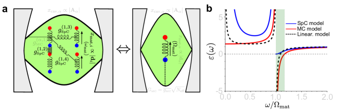
Figure 5: Interaction between matter excitations within a homogeneous material (here a homogeneous ensemble of molecules) and the transverse modes of a dielectric cavity. a) (Left) Schematic of the system. The oscillators $x_{\text{cav},\alpha}$ represent the vector potential $\mathbf{A}_{\alpha}$ associated to all modes $\alpha$ in the cavity, and the matter oscillators $x_{\text{mat},i}$ represent the dipole moments $\mathbf{d}_{i}$ of each molecule. The cavity-molecule interactions are modelled with the MC model and coupling strength $g_{\scriptscriptstyle{\text{MC}}}^{(\alpha,i)}$, and the molecule-molecule interactions with the SpC model and coupling strength $g_{\scriptscriptstyle{\text{SpC}}}^{(i,j)}$. We indicate all the interactions of the molecule with index $i=1$. (Right) Schematic indicating that the description of the full system is equivalent to the coupling, within the MC model, of the cavity mode $\alpha$ with a single molecular excitation of dipole moment $\mathbf{d}_{\alpha}$, modified frequency $\Omega_{\text{mat}}$ and modified coupling strength $G_{\scriptscriptstyle{\text{MC}}}$. b) Permittivity of the material inside the cavity, obtained from the classical SpC model (blue solid line, Eq. (37)), MC model (red solid line, Eq. (35)) and the linearized model (black dashed line, Eq. (38)), for the collective coupling strength $G=0.3\,\omega_{\text{cav}}$.

We have thus shown that the MC model constitutes the proper description of the coupling between transverse cavity modes and matter excitations in homogeneous materials. Next, we confirm the validity of this model to describe the system by demonstrating that it allows for recovering the typical bulk permittivity of phononic materials or ensembles of molecules, and that this is beyond the SpC or linearized models. We first note that, according to recent work [53, 80, 81], the dispersion of the cavity-matter system is exactly the same as the bulk dispersion of the material. This enables to relate the spectrum of the MC model with the bulk permittivity $\varepsilon(\omega)$ of the material in the following manner: the cavity modes of the bare cavity (without molecules) follow the dispersion of free photons as $\omega_{\text{cav},\alpha}=ck_{\alpha}$, with $c$ the light speed in vacuum and $k_{\alpha}$ the wavevector that is determined by the length $L_{\text{cav}}$ of the Fabry-Pérot cavity (for perfect mirrors) as $k_{\alpha}=n_{\alpha}\pi/L_{\text{cav}}$, for an integer $n_{\alpha}$. For the cavity filled with molecules, the frequency of each cavity mode of wavevector $k_{\alpha}$ is modified according to $\omega=\frac{ck_{\alpha}}{\sqrt{\varepsilon(\omega)}}=\frac{\omega_{\text{cav},\alpha}}{\sqrt{\varepsilon(\omega)}}$. According to the discussion above, these $\omega$ values need to be equal to the eigenfrequencies $\omega_{\pm,\scriptscriptstyle{\text{MC}}}$ of the MC model. By using the relation $\omega_{\pm,\scriptscriptstyle{\text{MC}}}(\omega_{\text{cav},\alpha})$ between these eigenfrequencies and the bare cavity frequencies from Eq. (6), we can obtain that the permittivity of the material in the cavity must be

$$\varepsilon_{\scriptscriptstyle{\text{MC}}}(\omega)=1+\frac{4G_{\scriptscriptstyle{\text{MC}}}^{2}}{\Omega_{\text{mat}}^{2}-\omega^{2}}.$$ (35)

The last expression can be compared, for example, with the permittivity of polar materials, which can often be described in a range of infrared frequencies by

$$\varepsilon(\omega)=\varepsilon_{\infty}\left(1+\frac{\omega_{\text{LO}}^{2}-\omega_{\text{TO}}^{2}}{\omega_{\text{TO}}^{2}-\omega^{2}}\right),$$ (36)

where $\omega_{\text{TO}}$ and $\omega_{\text{LO}}$ are the frequencies of the transverse optical and longitudinal optical phonons, respectively [82]. Thus, the MC model recovers the permittivity of a polar material or an ensemble of molecules, with the correspondences $\Omega_{\text{mat}}=\omega_{\text{TO}}$ and $G_{\scriptscriptstyle{\text{MC}}}=\sqrt{\frac{\omega_{\text{LO}}^{2}-\omega_{\text{TO}}^{2}}{4}}$. The only difference is that Eq. (35) does not include the high-frequency permittivity $\varepsilon_{\infty}$, because this parameter originates from other molecular excitations than the one considered in our model. In order to show that only the MC model correctly describes the permittivity of these materials, we derive the permittivities $\varepsilon_{\scriptscriptstyle{\text{SpC}}}(\omega)$ and $\varepsilon_{\scriptscriptstyle{\text{lin}}}(\omega)$ obtained within the SpC and linearized models, by repeating the procedure with Eqs. (3) and (8), respectively. We obtain:

$$\varepsilon_{\scriptscriptstyle{\text{SpC}}}(\omega)=\left(\frac{}{}\frac{2G_{\scriptscriptstyle{\text{SpC}}}^{2}\Omega_{\text{mat}}}{\omega(\Omega_{\text{mat}}^{2}-\omega^{2})}+\sqrt{1+\left(\frac{2G_{\scriptscriptstyle{\text{SpC}}}^{2}\Omega_{\text{mat}}}{\omega(\Omega_{\text{mat}}^{2}-\omega^{2})}\right)^{2}}\right)^{2},$$ (37)

$$\varepsilon_{\scriptscriptstyle{\text{lin}}}(\omega)=1+\frac{G_{\scriptscriptstyle{\text{lin}}}^{2}}{\omega(\Omega_{\text{mat}}-\omega)},$$ (38)

which do not follow the standard form of the permittivity (Eq. (36)).

For a comparison, we plot in Fig. 5b the permittivities obtained with the MC model (red solid line, Eq. (35)), the SpC model (blue solid line, Eq. (37)) and the linearized model (black dashed line, Eq. (38)), as a function of the normalized frequency $\omega/\Omega_{\text{mat}}$, with $G=0.3\,\Omega_{\text{mat}}$. The different behavior of the permittivity according to the three models can be clearly observed by comparing the Reststrahlen band, which corresponds to the range of frequencies with negative permittivity. In polar materials, this band is delimited by the phonon frequencies $\omega_{\text{TO}}$ and $\omega_{\text{LO}}$. The MC model describes the Reststrahlen band appropriately, because the permittivity is negative in the range $\omega\in\left(\Omega_{\text{mat}},\sqrt{\Omega_{\text{mat}}^{2}+4G_{\scriptscriptstyle{\text{MC}}}^{2}}\right)=(\omega_{\text{TO}},\omega_{\text{LO}})$ (highlighted by the green area in Fig. 5b). In contrast, the permittivity $\varepsilon_{\scriptscriptstyle{\text{SpC}}}$ associated to the SpC model is non-negative for all frequencies, and thus is unable to describe the presence of a Reststrahlen band. Although the linearized model does give a Reststrahlen band, as can be appreciated in Fig. 5b, the width of this band is half of that obtained with the MC model. As an additional difference between the models, only the MC model results in a permittivity that does not diverge in the $\omega\rightarrow 0$ limit, in agreement with the expected behavior (Eq. (36)).

We have focused in this subsection on the coupling with (harmonic) vibrations and phonons, but the discussion holds valid for other matter excitations, independently from their physical origin, such as molecular excitons. The main difference between excitons and vibrations is that the former are two-level systems (fermionic transitions), which for small number of molecules introduces many non-linear effects not included in classical harmonic oscillator models. However, when many molecules are present, the collective excitation is bosonic according to the Holstein-Primakoff transformation [83]. Therefore, while in Secs. 4.1 and 4.2 the discussion is valid for harmonic excitations such as vibrations or to obtain properties such as the eigenvalues of the system or the electric field distribution of the hybrid modes under weak illumination, the discussion of this subsection is applicable more broadly.

5 Conclusions

We have analyzed the application of classical coupled harmonic oscillator models to describe nanophotonic systems under ultrastrong coupling and the connection of these models with quantum descriptions. The study focuses on the two classical models typically used in this context, here referred to as the Spring Coupling (SpC) and Momentum Coupling (MC) models, where the difference relies on whether the coupling term is proportional to the displacement of the oscillators (SpC model) or to their time derivatives (MC model). The choice between these models typically does not have significant consequences in the weak and strong coupling regimes, where both can be approximated to the same linearized model (this approximation is equivalent to the rotating-wave approximation in quantum models). However, the SpC model and the MC model result in very different eigenvalues in the ultrastrong coupling regime. We demonstrate that the SpC model represents light-matter coupling via Coulomb interactions, such as those governing the interaction between different molecules and between molecules and small plasmonic nanoparticles, and that this model results in the same eigenvalue spectra as the quantum Hopfield Hamiltonian without diamagnetic term. On the other hand, the MC model reproduces the spectra of systems for which the diamagnetic term should be present in the Hamiltonian, corresponding to systems where matter excitations interact with transverse electromagnetic fields (for example, in conventional dielectric cavities). We thus show that the SpC and MC models are capable of capturing the same information than a cavity-QED description about the spectra of nanophotonic systems under ultrastrong coupling, but using a simpler framework. We generalize this discussion in the SI (Sec. S2) to other alternative models of classical oscillators.

Additionally, classical oscillator models are typically used to calculate the eigenvalues of the system, but we also discuss how they provide other experimentally measurable magnitudes in three canonical systems of nanophotonics. We first show that the MC model can be applied to calculate the electric field distribution of each hybrid mode in a dielectric cavity filled by a single molecule. On the other hand, for the SpC model, we consider a molecule situated near a metallic nanoparticle and calculate the near-field distribution and the far-field scattering spectra. Last, the two models are combined when considering an ensemble of molecules that interact with each other due to Coulomb interactions (SpC model) and also with transverse electromagnetic modes of a cavity (MC model). In this case, we show that the response of the system can be obtained by considering that each transverse cavity mode interacts with a collective molecular excitation. The only effect of the molecule-molecule interactions is to modify the effective frequency of these collective excitations, and the MC model describes the relevant ultrastrong coupling between these collective excitations and the cavity modes. Interestingly, only the MC model enables to recover correctly the permittivity of the material filling the cavity, and thus the Reststrahlen band observed in polar materials. Our work thus advances the exploration of classical descriptions of the ultrastrong coupling regime and opens the possibility to simplify the analysis of a wide variety of complex systems that are usually described with quantum models.

S1 Derivation of the equations of motion in the classical coupled harmonic oscillator models

In the main article, we compare classical models of coupled harmonic oscillators with Hamiltonians in the framework of cavity Quantum Electrodynamics (QED). In this supplementary section, we derive in detail the equations of motion of the classical harmonic oscillators from a purely classical description, without quantization. We start this derivation from the general classical Lagrangian representing charges and electromagnetic fields, which we then particularize for the specific systems that we analyze in the main article under ultrastrong coupling. Afterwards, we show that the Spring Coupling (SpC) and the Momentum Coupling (MC) models defined in the main article are obtained from the Euler-Lagrange equations of motion of these Lagrangians, demonstrating that a fully classical description is enough to obtain models of ultrastrong coupling without the need to use any quantum model.

The form of the electromagnetic Lagrangian depends on the gauge. We choose the Coulomb gauge, which leads to the following expression [1]:

$$L_{\text{Cou}}=\sum_{i}\frac{1}{2}m_{i}\dot{\mathbf{r}}_{i}^{2}-\sum_{i,j>i}\frac{q_{i}q_{j}}{4\pi\varepsilon_{0}|\mathbf{r}_{i}-\mathbf{r}_{j}|}+\int\left[\frac{\varepsilon_{0}}{2}(|\dot{\mathbf{A}}(\mathbf{r})|^{2}-c^{2}|\nabla\crossproduct\mathbf{A}(\mathbf{r})|^{2})+\mathbf{j}(\mathbf{r})\cdot\mathbf{A}(\mathbf{r})\right]d\mathbf{r}.$$ (S1)

In this Lagrangian, the electromagnetic degrees of freedom are encapsulated in the dynamical field variable $\mathbf{A}(\mathbf{r})$, which represents the vector potential of the fields, with the condition $\nabla\cdot\mathbf{A}=0$ due to the choice of gauge. The energy of these fields is scaled by the vacuum permitivity $\varepsilon_{0}$ and the light speed in vacuum $c$ (for simplicity, we assume in this section that the material filling the cavity is vacuum). On the other hand, all the dynamics related to the matter structure are expressed by the spatial positions $\mathbf{r}_{i}$ of each point-like charge indexed by $i$. Each point charge, of mass $m_{i}$ and charge $q_{i}$, interacts with all the others according to the Coulomb potential energy (second term in the right handside) and with the transverse electromagnetic fields as indicated in the last term of the Lagrangian (of the form $\mathbf{j}\cdot\mathbf{A}$), where $\mathbf{j}(\mathbf{r})=\sum_{i}q_{i}\dot{\mathbf{r}}_{i}\delta(\mathbf{r}-\mathbf{r}_{i})$ is the current density at any position $\mathbf{r}$.

The equations of motion obtained from the Lagrangian in Eq. (S1) for the variables $\mathbf{A}(\mathbf{r})$ and $\mathbf{r}_{i}$ are completely equivalent to Maxwell’s equation for a general system. We are interested in obtaining the equations of motion that describe the dynamics of systems formed by molecules interacting with cavity modes in the strong and the ultrastrong coupling regimes. First, we focus on the terms of the Lagrangian related to the electromagnetic field (which in the Coulomb gauge is entirely described with the vector potential $\mathbf{A}$), in order to separate them into the contribution of different cavity modes. The vector potential is separated into the components $\mathbf{A}_{\alpha}(\mathbf{r})$ of all transverse modes $\alpha$ of the cavity as $\mathbf{A}(\mathbf{r})=\sum_{\alpha}\mathbf{A}_{\alpha}(\mathbf{r})=\sum_{\alpha}\mathcal{A}_{\alpha}\Xi_{\alpha}(\mathbf{r})\mathbf{n}_{\alpha}$. For each $\alpha$ index, the field is polarized in the direction determined by the unit vector $\mathbf{n}_{\alpha}$, the amplitude is given by $\mathcal{A}_{\alpha}$ and the fields have spatial distribution $\Xi_{\alpha}(\mathbf{r})$, normalized so that $\Xi_{\alpha}(\mathbf{r})=1$ in the position where the field is maximum. Further, we consider that the $\alpha$ modes form an orthogonal basis and the integral of the field distribution over space gives the effective volume of the mode, i.e.

$$\int\Xi_{\alpha}(\mathbf{r})\Xi^{*}_{\alpha^{\prime}}(\mathbf{r})d\mathbf{r}=V_{\text{eff},\alpha}\delta_{\alpha,\alpha^{\prime}}.$$ (S2)

By taking into account the decomposition of the modes and their orthogonality, the terms of the Lagrangian of Eq. (S1) only related to the electromagnetic fields are written as

$$\int\frac{\varepsilon_{0}}{2}\left(\left|\sum_{\alpha}\dot{\mathcal{A}}_{\alpha}\Xi_{\alpha}(\mathbf{r})\mathbf{n}_{\alpha}\right|^{2}-c^{2}\left|\nabla\crossproduct\sum_{\alpha}\mathcal{A}_{\alpha}\Xi_{\alpha}(\mathbf{r})\mathbf{n}_{\alpha}\right|^{2}\right)d\mathbf{r}=\sum_{\alpha}\frac{\varepsilon_{0}V_{\text{eff},\alpha}}{2}\left(\dot{\mathcal{A}}_{\alpha}\dot{\mathcal{A}}^{*}_{\alpha}-\omega_{\text{cav},\alpha}^{2}\mathcal{A}_{\alpha}\mathcal{A}^{*}_{\alpha}\right).$$ (S3)

We now focus on the terms of the Lagrangian associated to the matter degrees of freedom, so that we can describe the matter excitations. We model the material as an ensemble of dipoles indexed by $j$, each formed by two point charges that have the same mass $m_{j}$ and opposite charges, and are placed in positions $\mathbf{r}_{j+}$ and $\mathbf{r}_{j-}$. The two point charges are at equilibrium if they are placed at a distance $|\mathbf{r}_{j+}-\mathbf{r}_{j-}|=|\mathbf{r}_{\text{eq}}|$. We make the harmonic approximation to the Coulomb potential of each dipole with respect to the equilibrium position: $\frac{q_{j}^{2}}{4\pi\varepsilon_{0}|\mathbf{r}_{j+}-\mathbf{r}_{j-}|}=\frac{1}{2}m_{\text{red}}\omega_{\text{mat}}^{2}|\mathbf{r}_{j+}-\mathbf{r}_{j-}-\mathbf{r}_{\text{eq}}|^{2}+\mathcal{O}(|\mathbf{r}_{j+}-\mathbf{r}_{j-}-\mathbf{r}_{\text{eq}}|^{3})\approx\frac{1}{2}m_{\text{red}}\omega_{\text{mat}}^{2}|\mathbf{r}_{j+}-\mathbf{r}_{j-}-\mathbf{r}_{\text{eq}}|^{2}$, where $m_{\text{red}}=\frac{m_{j}}{2}$ is the reduced mass of the dipole. We also assume that the mass center of the dipole is static at position $\mathbf{r}_{j}=\frac{\mathbf{r}_{j+}+\mathbf{r}_{j-}}{2}$. Therefore, the only variable that evolves in time for each dipole is the distance between point charges from the equilibrium position, i.e., $\mathbf{l}_{j}=\mathbf{r}_{j+}-\mathbf{r}_{j-}-\mathbf{r}_{\text{eq}}$ or, equivalently, the induced dipole moment $\mathbf{d}_{j}=q_{j}\mathbf{l}_{j}.$ From these assumptions, the Coulomb potential energy in Eq. (S1) includes the harmonic potential energy corresponding to the charges in each dipole, and also the potential energy due to the interaction between different dipoles. Accordingly, the terms related to the matter degrees of freedom in the Lagrangian transform as

$$\sum_{j}\frac{1}{2}m_{j}\dot{\mathbf{r}}_{j}^{2}-\sum_{i,j>i}\frac{q_{i}q_{j}}{4\pi\varepsilon_{0}|\mathbf{r}_{i}-\mathbf{r}_{j}|}= \sum_{j}\left(\frac{1}{2}\frac{m_{\text{red},j}}{q_{j}^{2}}\dot{d}_{j}^{2}-\frac{1}{2}\frac{m_{\text{red},j}}{q_{j}^{2}}\omega_{\text{mat},j}^{2}d_{j}^{2}\right)$$

$$-\sum_{i,j>i}\frac{1}{4\pi\varepsilon_{0}|\mathbf{r}_{i}-\mathbf{r}_{j}|^{3}}\left[\mathbf{d}_{i}\cdot\mathbf{d}_{j}-3(\mathbf{d}_{i}\cdot\mathbf{n}_{\mathbf{r}ij})(\mathbf{d}_{j}\cdot\mathbf{n}_{\mathbf{r}ij})\right],$$ (S4)

with $d_{j}=|\mathbf{d}_{j}|$ and the unit vector $\mathbf{n}_{\mathbf{r}ij}=\frac{\mathbf{r}_{j}-\mathbf{r}_{i}}{|\mathbf{r}_{j}-\mathbf{r}_{i}|}$.

Equation (S4) has been derived using the harmonic approximation of the dipolar potential, and as a consequence all terms of the Lagrangian that do not account for light-matter interaction are quadratic with respect to the amplitudes of the vector potential and their time derivatives (Eq. (S3)), or with respect to the dipole moments and their time derivatives (Eq. (S4)). Therefore, if light and matter were uncoupled, the dynamical evolution of these variables would be the same as that of free harmonic oscillators. We now discuss how the interaction between the cavity modes and the dipoles affects the equations of motion. The coupling of each dipole with the transverse fields of the cavity appears in the Lagrangian as

$$\int\mathbf{j}\cdot\mathbf{A}\;d\mathbf{r} =\int\left(\sum_{j}q_{j}\dot{\mathbf{r}}_{j+}\delta(\mathbf{r}-\mathbf{r}_{j+})-q_{j}\dot{\mathbf{r}}_{j-}\delta(\mathbf{r}-\mathbf{r}_{j-})\right)\left(\sum_{\alpha}\mathcal{A}_{\alpha}\Xi_{\alpha}(\mathbf{r})\mathbf{n}_{\alpha}\right)d\mathbf{r}$$

$$=\sum_{j,\alpha}q_{j}[\mathbf{r}_{j+}\Xi_{\alpha}(\dot{\mathbf{r}}_{j+})-\dot{\mathbf{r}}_{j-}\Xi_{\alpha}(\mathbf{r}_{j-})]\mathcal{A}_{\alpha}\mathbf{n}_{\alpha}\approx\sum_{j,\alpha}\mathcal{A}_{\alpha}\Xi_{\alpha}(\mathbf{r}_{j})\dot{\mathbf{d}}_{j}\cdot\mathbf{n}_{\alpha}$$ (S5)

In the last step, we have performed the long-wavelength approximation, so that in the length scale of each dipole the fields do not vary, i.e. $\Xi(\mathbf{r}_{j+})\approx\Xi(\mathbf{r}_{j-})$ for any $j$. The total Lagrangian of the system in the Coulomb gauge reads

$$L_{\text{Cou}}(d_{j},\dot{d}_{j},\mathcal{A}_{\alpha},\dot{\mathcal{A}}_{\alpha},\mathcal{A}^{*}_{\alpha},\dot{\mathcal{A}}^{*}_{\alpha})= \sum_{\alpha}\frac{\varepsilon_{0}V_{\text{eff},\alpha}}{2}\left(\dot{\mathcal{A}}_{\alpha}\dot{\mathcal{A}}^{*}_{\alpha}-\omega_{\text{cav},\alpha}^{2}\mathcal{A}_{\alpha}\mathcal{A}^{*}_{\alpha}\right)+\sum_{j}\frac{1}{2}\frac{1}{f_{\text{mat},j}}\left(\dot{d}_{j}^{2}-\omega_{\text{mat},j}^{2}d_{j}^{2}\right)$$

$$+ \sum_{j,\alpha}\mathcal{A}_{\alpha}\dot{d}_{j}\Xi_{\alpha}(\mathbf{r}_{j})\cos\theta_{\alpha,j}-\sum_{i,j}d_{i}d_{j}\frac{\mathbf{n}_{\mathbf{d}i}\cdot\mathbf{n}_{\mathbf{d}j}-3(\mathbf{n}_{\mathbf{d}i}\cdot\mathbf{n}_{\mathbf{r}ij})(\mathbf{n}_{\mathbf{d}j}\cdot\mathbf{n}_{\mathbf{r}ij})}{4\pi\varepsilon_{0}|\mathbf{r}_{i}-\mathbf{r}_{j}|^{3}},$$ (S6)

where $\mathbf{n}_{\mathbf{d}j}=\frac{\mathbf{d}_{j}}{|\mathbf{d}_{j}|}$, $\theta_{\alpha,j}$ is the angle between the dipole moment $\mathbf{d}_{j}$ and the direction $\mathbf{n}_{\alpha}$ of the electric field in the mode $\alpha$, and $f_{\text{mat}}=\frac{q_{j}^{2}}{m_{\text{red}}}$ is the oscillator strength of the $j^{\text{th}}$ dipole.

From the Lagrangian $L_{\text{Cou}}$ of Eq. (S6), we can easily derive the equations of motion of the classical coupled harmonic oscillators by calculating the Euler-Lagrange equations, $\frac{d}{dt}\frac{\partial L_{\text{Cou}}}{\partial\dot{x}}-\frac{\partial L_{\text{Cou}}}{\partial x}=0$, for $x\in\{d_{j},\mathcal{A}^{*}_{\alpha}\}$. The resulting equations of motion are

$$\ddot{\mathcal{A}}_{\alpha}+\omega_{\text{cav},\alpha}^{2}\mathcal{A}_{\alpha}-\sum_{j}\dot{d}_{j}\frac{\Xi_{\alpha}(\mathbf{r}_{j})\cos\theta_{\alpha,j}}{\varepsilon_{0}V_{\text{eff},\alpha}}=0,$$ (S7a)

$$\ddot{d}_{j}+\omega_{\text{mat},j}^{2}d_{j}+f_{\text{mat},j}\sum_{i\neq j}\frac{\mathbf{n}_{\mathbf{d}i}\cdot\mathbf{n}_{\mathbf{d}j}-3(\mathbf{n}_{\mathbf{d}i}\cdot\mathbf{n}_{\mathbf{r}ij})(\mathbf{n}_{\mathbf{d}j}\cdot\mathbf{n}_{\mathbf{r}ij})}{4\pi\varepsilon_{0}|\mathbf{r}_{i}-\mathbf{r}_{j}|^{3}}d_{i}+\sum_{\alpha}\dot{\mathcal{A}}_{\alpha}f_{\text{mat},j}\Xi^{*}_{\alpha}(\mathbf{r}_{j})\cos\theta_{\alpha,j}=0.$$ (S7b)

These equations account for all dipole-cavity and dipole-dipole interactions, as analyzed in Sec. 4.3 of the main article. To show how each interaction is connected with the MC and SpC models, we focus on the two canonical examples analyzed in Secs. 4.1 and 4.2 of the main article:

• Coupling between a molecule and a transverse mode of a dielectric cavity (Section 4.1): By considering a single transverse mode $\alpha$ of the cavity interacting with one molecule represented by the induced dipole moment $d$, all Coulomb interactions in Eq. (S7) are eliminated. The equations of motion become

  $$\ddot{\mathcal{A}}+\omega_{\text{cav}}^{2}\mathcal{A}-\dot{d}\frac{\Xi(\mathbf{r}_{\text{mat}})\cos\theta}{\varepsilon_{0}V_{\text{eff}}}=0,$$ (S8a)

  $$\ddot{d}+\omega_{\text{mat}}^{2}d+\dot{\mathcal{A}}f_{\text{mat}}\Xi^{*}(\mathbf{r}_{\text{mat}})\cos\theta=0.$$ (S8b)

  By replacing here the oscillator amplitudes $x_{\text{cav}}=\mathcal{A}\sqrt{\varepsilon_{0}V_{\text{eff}}}$ and $x_{\text{mat}}=\frac{d}{\sqrt{f_{\text{mat}}}}$ and the coupling strength

  $$g_{\scriptscriptstyle{\text{MC}}}=\frac{1}{2}\sqrt{\frac{f_{\text{mat}}}{\varepsilon_{0}V_{\text{eff}}}}\Xi(\mathbf{r}_{\text{mat}})\cos\theta,$$ (S9)

  we recover the equations of motion of the MC model (Eq. (4b) in the main article).

• Coupling between a molecule and a plasmonic nanoparticle via Coulomb interactions (Section 4.2): We consider that the molecule and the nanoparticle have dipole moments $d_{\text{mat}}$ and $d_{\text{cav}}$, respectively. Under the quasitatic approximation of the plasmonic response, the vector potential components of all transverse modes are neglected. With this approximation and for only two dipoles, Eq. (S7) is written as

  $$\ddot{d}_{\text{cav}}+\omega_{\text{cav}}^{2}d_{\text{cav}}+f_{\text{cav}}\frac{\mathbf{n}_{\mathbf{d}\text{cav}}\cdot\mathbf{n}_{\mathbf{d}\text{mat}}-3(\mathbf{n}_{\mathbf{d}\text{cav}}\cdot\mathbf{n}_{\mathbf{r}\text{rel}})(\mathbf{n}_{\mathbf{d}\text{mat}}\cdot\mathbf{n}_{\mathbf{r}\text{rel}})}{4\pi\varepsilon_{0}|\mathbf{r}_{\text{cav}}-\mathbf{r}_{\text{mat}}|^{3}}d_{\text{mat}}=0,$$ (S10a)

  $$\ddot{d}_{\text{mat}}+\omega_{\text{mat}}^{2}d_{\text{mat}}+f_{\text{mat}}\frac{\mathbf{n}_{\mathbf{d}\text{cav}}\cdot\mathbf{n}_{\mathbf{d}\text{mat}}-3(\mathbf{n}_{\mathbf{d}\text{cav}}\cdot\mathbf{n}_{\mathbf{r}\text{rel}})(\mathbf{n}_{\mathbf{d}\text{mat}}\cdot\mathbf{n}_{\mathbf{r}\text{rel}})}{4\pi\varepsilon_{0}|\mathbf{r}_{\text{cav}}-\mathbf{r}_{\text{mat}}|^{3}}d_{\text{cav}}=0,$$ (S10b)

  where $\mathbf{n}_{\mathbf{r}\text{rel}}=\frac{\mathbf{r}_{\text{cav}}-\mathbf{r}_{\text{mat}}}{|\mathbf{r}_{\text{cav}}-\mathbf{r}_{\text{mat}}|}$ is the unitary vector of the relative direction between the nanocavity and the molecule. By replacing $x_{\text{cav}}=\frac{d_{\text{cav}}}{\sqrt{f_{\text{cav}}}}$ and $x_{\text{mat}}=\frac{d_{\text{mat}}}{\sqrt{f_{\text{mat}}}}$, together with the coupling strength $g_{\scriptscriptstyle{\text{SpC}}}$ defined as

  $$g_{\scriptscriptstyle{\text{SpC}}}=\frac{1}{2}\frac{\sqrt{f_{\text{cav}}}\sqrt{f_{\text{mat}}}}{4\pi\varepsilon_{0}|\mathbf{r}_{\text{cav}}-\mathbf{r}_{\text{mat}}|^{3}\sqrt{\omega_{\text{cav}}\omega_{\text{mat}}}}[\mathbf{n}_{\mathbf{d}\text{cav}}\cdot\mathbf{n}_{\mathbf{d}\text{mat}}-3(\mathbf{n}_{\mathbf{d}\text{cav}}\cdot\mathbf{n}_{\mathbf{r}\text{rel}})(\mathbf{n}_{\mathbf{d}\text{mat}}\cdot\mathbf{n}_{\mathbf{r}\text{rel}})],$$ (S11)

  we recover the equations of the SpC model (Eq. (2b) in the main article).

Spring coupling model with external laser illumination

In Sec. 4.2 of the main text, the dipolar mode of a metallic nanoparticle is excited by an external laser. We now discuss briefly how to introduce an incident laser field in the model of nanocavity-molecule interaction (however, this derivation can be generalized to systems with more molecules, with metallic nanoparticles suporting more plasmonic modes, and also to a dielectric cavity supporting transverse cavity modes). The incident field has associated a vector potential of the form $\mathbf{A}_{\text{inc}}(\mathbf{r},t)=\mathcal{A}_{\text{inc}}e^{i\mathbf{k}_{\text{inc}}\cdot\mathbf{r}}e^{-i\omega t}$, which is a planewave of wavevector $\mathbf{k}_{\text{inc}}$, amplitude $\mathcal{A}_{\text{inc}}$ and frequency $\omega$. Under the quasistatic appoximation, all transverse modes $\alpha$ of the system are neglected, and thus the only component of the vector potential considered in the Lagrangian of Eq. (S6) corresponds to the external laser $\mathbf{A}_{\text{inc}}(\mathbf{r},t)$. With these considerations, the Lagrangian of Eq. (S6) becomes

$$L_{\text{Cou}}^{\text{dip-dip}}(d_{\text{cav}},\dot{d}_{\text{cav}},d_{\text{mat}},\dot{d}_{\text{mat}})=\frac{1}{2}\frac{1}{f_{\text{cav}}}\left(\dot{d}_{\text{cav}}^{2}-\omega_{\text{cav}}^{2}d_{\text{cav}}^{2}\right)+\frac{1}{2}\frac{1}{f_{\text{mat}}}\left(\dot{d}_{\text{mat}}^{2}-\omega_{\text{mat}}^{2}d_{\text{mat}}^{2}\right)$$

$$-d_{\text{cav}}d_{\text{mat}}\frac{\mathbf{n}_{\mathbf{d}\text{cav}}\cdot\mathbf{n}_{\mathbf{d}\text{mat}}-3(\mathbf{n}_{\mathbf{d}\text{cav}}\cdot\mathbf{n}_{\mathbf{r}\text{rel}})(\mathbf{n}_{\mathbf{d}\text{mat}}\cdot\mathbf{n}_{\mathbf{r}\text{rel}})}{4\pi\varepsilon_{0}|\mathbf{r}_{\text{cav}}-\mathbf{r}_{\text{mat}}|^{3}}+\mathcal{A}_{\text{inc}}e^{-i\omega t}(\dot{d}_{\text{cav}}\cos\theta_{\text{inc},\text{cav}}+\dot{d}_{\text{mat}}\cos\theta_{\text{inc},\text{mat}}),$$ (S12)

where $\theta_{\text{inc},\text{cav}}$ and $\theta_{\text{inc},\text{mat}}$ are the angles between the incident field and the dipole moments of the cavity and molecule, respectively. The superscript ”dip-dip” emphasizes that we only consider dipole-dipole interactions for this system (under the quasistatic approximation). The dynamics of the variables $d_{\text{cav}}$ and $d_{\text{mat}}$ are obtained within the Euler-Lagrange equations from Eq. (S12). By calculating these equations of motion and transforming the variables into the oscillator amplitudes $x_{\text{cav}}=\frac{d_{\text{cav}}}{\sqrt{f_{\text{cav}}}}$ and $x_{\text{mat}}=\frac{d_{\text{mat}}}{\sqrt{f_{\text{mat}}}}$, the resulting equations are

$$\ddot{x}_{\text{cav}}+\omega_{\text{cav}}^{2}x_{\text{cav}}+\frac{\mathbf{n}_{\mathbf{d}\text{cav}}\cdot\mathbf{n}_{\mathbf{d}\text{mat}}-3(\mathbf{n}_{\mathbf{d}\text{cav}}\cdot\mathbf{n}_{\mathbf{r}\text{rel}})(\mathbf{n}_{\mathbf{d}\text{mat}}\cdot\mathbf{n}_{\mathbf{r}\text{rel}})}{4\pi\varepsilon_{0}|\mathbf{r}_{\text{cav}}-\mathbf{r}_{\text{mat}}|^{3}}x_{\text{mat}}=i\omega\mathcal{A}_{\text{inc}}\sqrt{f_{\text{cav}}}\cos\theta_{\text{inc},\text{cav}}e^{-i\omega t},$$ (S13a)

$$\ddot{x}_{\text{mat}}+\omega_{\text{mat}}^{2}x_{\text{mat}}+\frac{\mathbf{n}_{\mathbf{d}\text{cav}}\cdot\mathbf{n}_{\mathbf{d}\text{mat}}-3(\mathbf{n}_{\mathbf{d}\text{cav}}\cdot\mathbf{n}_{\mathbf{r}\text{rel}})(\mathbf{n}_{\mathbf{d}\text{mat}}\cdot\mathbf{n}_{\mathbf{r}\text{rel}})}{4\pi\varepsilon_{0}|\mathbf{r}_{\text{cav}}-\mathbf{r}_{\text{mat}}|^{3}}x_{\text{cav}}=i\omega\mathcal{A}_{\text{inc}}\sqrt{f_{\text{mat}}}\cos\theta_{\text{inc},\text{mat}}e^{-i\omega t}.$$ (S13b)

Therefore, the incident field is incorporated into the SpC equations of motion (Eq. (2b) in the main article) by adding time-dependent forces of amplitude $F_{\text{cav}}=i\omega\mathcal{A}_{\text{inc}}\sqrt{f_{\text{cav}}}\cos\theta_{\text{inc},\text{cav}}$ and $F_{\text{mat}}=i\omega\mathcal{A}_{\text{inc}}\sqrt{f_{\text{mat}}}\cos\theta_{\text{inc},\text{mat}}$ to the nanocavity and the molecule, respectively.

Classical description of the coupling between a molecule and a plasmonic nanocavity based on their polarizability

The interaction of a small metallic nanoparticle with a molecular excitation can also be described classically by using polarizabilities $\alpha_{\text{cav}}$ and $\alpha_{\text{mat}}$ for both particles, so that the dipole moment induced by the electric field at each position $\mathbf{r}_{\text{cav}}$ and $\mathbf{r}_{\text{mat}}$ is given by $\mathbf{d}_{\text{cav}}=\alpha_{\text{cav}}\mathbf{E}(\mathbf{r}_{\text{cav}})$ and $\mathbf{d}_{\text{mat}}=\alpha_{\text{mat}}\mathbf{E}(\mathbf{r}_{\text{mat}})$, respectively. We briefly show here that this approach leads to the same equations as the SpC model obtained from the electromagnetic Lagrangian, which supports the validity of the general approach used in the main text. For the cavity (metallic nanoparticle) and the molecular excitation (or any matter excitation in general), we consider the polarizability given by the Lorentz oscillator model. In the case of the molecule, we focus on a single excitation with Lorentzian polarizability centered at resonant frequency $\omega_{\text{mat}}$, linewidth determined by the damping frequency $\gamma$ and oscillator strength $f_{\text{mat}}$. Similarly, we also model the nanocavity response as given by a single plasmonic resonance that follows a Lorentzian-like lineshape, which is the typical lineshape in the quasistatic regime. This resonance is centered at frequency $\omega_{\text{cav}}$, and is characterized by losses $\kappa$ and oscillator strength $f_{\text{cav}}$. The polarizabilities of the plasmonic nanocavity and the molecule are then given by

$$\alpha_{\text{cav}}(\omega)=\frac{f_{\text{cav}}}{\omega_{\text{cav}}^{2}-\omega^{2}-i\omega\kappa},$$ (S14a)

$$\alpha_{\text{mat}}(\omega)=\frac{f_{\text{mat}}}{\omega_{\text{mat}}^{2}-\omega^{2}-i\omega\gamma}.$$ (S14b)

The dipole moment of each particle is induced by the electric field $\mathbf{E}_{\text{inc}}$ of the external laser and also by the electric field generated by the other particle ($\mathbf{E}_{\text{cav}}$ and $\mathbf{E}_{\text{mat}}$ corresponding to the fields induced by the nanocavity and the matter excitation, respectively). We then have $\mathbf{d}_{\text{cav}}=\alpha_{\text{cav}}[\mathbf{E}_{\text{mat}}(\mathbf{r}_{\text{cav}})+\mathbf{E}_{\text{inc}}]$ and $\mathbf{d}_{\text{mat}}=\alpha_{\text{mat}}[\mathbf{E}_{\text{cav}}(\mathbf{r}_{\text{mat}})+\mathbf{E}_{\text{inc}}]$. By inserting in these expressions the polarizabilities given by Eq. (S14b) and the fields induced by the dipoles excited at the cavity and the molecule,

$$\mathbf{E}_{\text{mat}}(\mathbf{r}_{\text{cav}})=\frac{\mathbf{n}_{\mathbf{d}\text{mat}}-3(\mathbf{n}_{\mathbf{d}\text{mat}}\cdot\mathbf{n}_{\mathbf{r}\text{rel}})\mathbf{n}_{\mathbf{r}\text{rel}}}{4\pi\varepsilon_{0}|\mathbf{r}_{\text{cav}}-\mathbf{r}_{\text{mat}}|^{3}}d_{\text{mat}},$$ (S15a)

$$\mathbf{E}_{\text{cav}}(\mathbf{r}_{\text{mat}})=\frac{\mathbf{n}_{\mathbf{d}\text{cav}}-3(\mathbf{n}_{\mathbf{d}\text{cav}}\cdot\mathbf{n}_{\mathbf{r}\text{rel}})\mathbf{n}_{\mathbf{r}\text{rel}}}{4\pi\varepsilon_{0}|\mathbf{r}_{\text{cav}}-\mathbf{r}_{\text{mat}}|^{3}}d_{\text{cav}},$$ (S15b)

we obtain the expressions of the induced dipole moments

$$(\omega_{\text{cav}}^{2}-\omega^{2}-i\omega\kappa)d_{\text{cav}}=f_{\text{cav}}\left[\frac{\mathbf{n}_{\mathbf{d}\text{cav}}\cdot\mathbf{n}_{\mathbf{d}\text{mat}}-3(\mathbf{n}_{\mathbf{d}\text{cav}}\cdot\mathbf{n}_{\mathbf{r}\text{rel}})(\mathbf{n}_{\mathbf{d}\text{mat}}\cdot\mathbf{n}_{\mathbf{r}\text{rel}})}{4\pi\varepsilon_{0}|\mathbf{r}_{\text{cav}}-\mathbf{r}_{\text{mat}}|^{3}}d_{\text{mat}}+\mathbf{E}_{\text{inc}}\cdot\mathbf{n}_{\mathbf{d}\text{cav}}\right],$$ (S16a)

$$(\omega_{\text{mat}}^{2}-\omega^{2}-i\omega\gamma)d_{\text{mat}}=f_{\text{mat}}\left[\frac{\mathbf{n}_{\mathbf{d}\text{cav}}\cdot\mathbf{n}_{\mathbf{d}\text{mat}}-3(\mathbf{n}_{\mathbf{d}\text{cav}}\cdot\mathbf{n}_{\mathbf{r}\text{rel}})(\mathbf{n}_{\mathbf{d}\text{mat}}\cdot\mathbf{n}_{\mathbf{r}\text{rel}})}{4\pi\varepsilon_{0}|\mathbf{r}_{\text{cav}}-\mathbf{r}_{\text{mat}}|^{3}}d_{\text{cav}}+\mathbf{E}_{\text{inc}}\cdot\mathbf{n}_{\mathbf{d}\text{mat}}\right].$$ (S16b)

These equations are equivalent to Eq. (S13b) in frequency domain, with $x_{\text{cav}}=\frac{d_{\text{cav}}}{\sqrt{f_{\text{cav}}}}$, $x_{\text{mat}}=\frac{d_{\text{mat}}}{\sqrt{f_{\text{mat}}}}$ and using the relation $|\mathbf{E}_{\text{inc}}|=|i\omega\mathcal{A_{\text{inc}}}|$ that follows from the definition of the vector potential.

S2 Alternative classical models of coupled harmonic oscillators

The discussion of Supplementary Sec. S1 led us to conclude that the classical MC model relates matter excitations with transverse electromagnetic modes, while the SpC model can express dipole-dipole interactions. In this supplementary section, we show that there are other classical coupled harmonic oscillator models that are equivalent to the MC and the SpC models. These alternative models depend on the gauge chosen for the classical Lagrangian and Hamiltonian descriptions, and we discuss oscillator models in two of the most vastly used gauges: the Coulomb and dipole gauges.

S2.1 Alternative model of a molecular excitation interacting with transverse cavity modes obtained within the Coulomb gauge

We first focus on the description of the coupling between a transverse electromagnetic mode and a molecular excitation, which is the system discussed in Sec. 4.1 of the main article. To obtain the equations of motion of this system, we start with the Lagrangian of Coulomb gauge given by Eq. (S6), which for the considered system gives the classical Lagrangian

$$L_{\text{Cou}}^{\text{min-c}}(d,\dot{d},\mathcal{A},\dot{\mathcal{A}})=\frac{\varepsilon_{0}V_{\text{eff}}}{2}(\dot{\mathcal{A}}^{2}-\omega_{\text{cav}}^{2}\mathcal{A}^{2})+\frac{1}{2f_{\text{mat}}}(\dot{d}^{2}-\omega_{\text{mat}}^{2}d^{2})+\mathcal{A}\dot{d}.$$ (S17)

Further, to simplify the analytical expressions in the following discussion, Eq. (S17) considers a specific case where the molecule is placed in the position of maximum field of the mode and oriented in the same direction as the field polarization, so that we set $\Xi(\mathbf{r_{\text{mat}}})\cos\theta=1$. However, the discussion of this section remains valid for other values of $\Xi(\mathbf{r_{\text{mat}}})\cos\theta.$

It has been shown in Supplementary Sec. S1 that the Euler-Lagrange equations derived from Eq. (S17) lead to the MC model. Alternatively, here we use Hamilton’s equations to obtain another equivalent classical model of harmonic oscillators. To first derive the classical Hamiltonian of the system, we obtain the canonical momenta related to the transverse electromagnetic modes and to the dipole moment in the Coulomb gauge as

$$\Pi_{\text{Cou}}= \frac{\partial L_{\text{Cou}}}{\partial\dot{\mathcal{A}}}=\varepsilon_{0}V_{\text{eff}}\dot{\mathcal{A}},$$ (S18a)

$$p_{\text{Cou}}= \frac{\partial L_{\text{Cou}}}{\partial\dot{d}}=\frac{\dot{d}}{f_{\text{mat}}}+\mathcal{A}.$$ (S18b)

According to these expressions, the dynamical variable $\Pi_{\text{Cou}}$ expresses the transverse electric field of the cavity modes from the relation $\mathbf{E}=-\frac{\partial\mathbf{A}}{\partial t}$. On the other hand, the relation between the dipole moment $d$ and its canonical momentum $p_{\text{Cou}}$ is more complicated because $p_{\text{Cou}}$ depends not only on $d$ but also on the vector potential. Using Eq. (S18), the calculation of the Hamiltonian $H^{\text{min-c}}_{\text{Cou}}=\dot{\mathcal{A}}\Pi_{\text{Cou}}+\dot{d}p_{\text{Cou}}-L^{\text{min-c}}_{\text{Cou}}$ is straightforward:

$$H_{\text{Cou}}^{\text{min-c}}= \frac{\Pi_{\text{Cou}}^{2}}{2\varepsilon_{0}V_{\text{eff}}}+\frac{1}{2}\varepsilon_{0}V_{\text{eff}}\omega_{\text{cav}}^{2}\mathcal{A}^{2}+\frac{f_{\text{mat}}}{2}p_{\text{Cou}}^{2}+\frac{1}{2}\frac{\omega_{\text{mat}}^{2}}{f_{\text{mat}}}d^{2}-f_{\text{mat}}p_{\text{Cou}}\mathcal{A}+\frac{1}{2}f_{\text{mat}}\mathcal{A}^{2}.$$ (S19)

This expression has the well-known form of the minimal-coupling Hamiltonian, and thus we refer to this form of the coupling with the superindex ”min-c” in the Lagrangian of Eq. (S17) and in the Hamiltonian of Eq. (S19). We can directly derive the Hamilton’s equations of motion of all canonical variables:

$$\dot{\mathcal{A}}=\frac{\partial H^{\text{min-c}}_{\text{Cou}}}{\partial\Pi_{\text{Cou}}}=\frac{\Pi_{\text{Cou}}}{\varepsilon_{0}V_{\text{eff}}},$$ (S20a)

$$\dot{\Pi}_{\text{Cou}}=-\frac{\partial H^{\text{min-c}}_{\text{Cou}}}{\partial\mathcal{A}}=-\varepsilon_{0}V_{\text{eff}}\omega_{\text{cav}}^{2}\mathcal{A}+f_{\text{mat}}(p_{\text{Cou}}-\mathcal{A}),$$ (S20b)

$$\dot{d}=\frac{\partial H^{\text{min-c}}_{\text{Cou}}}{\partial p_{\text{Cou}}}=f_{\text{mat}}(p_{\text{Cou}}-\mathcal{A}),$$ (S20c)

$$\dot{p}_{\text{Cou}}=-\frac{\partial H^{\text{min-c}}_{\text{Cou}}}{\partial d}=-\frac{\omega_{\text{mat}}^{2}}{f_{\text{mat}}}d_{j}.$$ (S20d)

Hamilton’s equations can be used to obtain classical harmonic oscillator models by eliminating two variables, which leads to two second-order differential equations. By choosing the variables $\mathcal{A}$ and $d$ to describe the dynamics of the system, we obtain

$$\ddot{\mathcal{A}}+\omega_{\text{cav}}^{2}\mathcal{A}-\frac{\dot{d}}{\varepsilon_{0}V_{\text{eff}}}=0,$$ (S21a)

$$\ddot{d}+\omega_{\text{mat}}^{2}d+f_{\text{mat}}\dot{\mathcal{A}}=0.$$ (S21b)

As discussed in detail in the main article, these equations have the form of the MC model, because the coupling terms are proportional to the time derivatives $\dot{\mathcal{A}}$ and $\dot{d}$. However, there are other possible ways to represent the response of this system with harmonic oscillators. An alternative is to choose the variable $p_{\text{Cou}}$ for the matter excitation and $\mathcal{A}$ for the cavity mode. By eliminating the rest of variables in Eq. (S20), the equations of motion for the chosen variables are written as

$$\ddot{\mathcal{A}}+\left(\omega_{\text{cav}}^{2}+\frac{f_{\text{mat}}}{\varepsilon_{0}V_{\text{eff}}}\right)\mathcal{A}-\frac{f_{\text{mat}}}{\varepsilon_{0}V_{\text{eff}}}p_{\text{Cou}}=0,$$ (S22a)

$$\ddot{p}_{\text{Cou}}+\omega_{\text{mat}}^{2}p_{\text{Cou}}-\omega_{\text{mat}}^{2}\mathcal{A}=0.$$ (S22b)

With the transformation $x_{\text{cav}}=\sqrt{\varepsilon_{0}V_{\text{eff}}}\mathcal{A}$ used in Sec. 4.1 of the main text, and with the new transformation $x^{\prime}_{\text{mat}}=\frac{\sqrt{f_{\text{mat}}}}{\omega_{\text{mat}}}p_{\text{Cou}}$, Eq. (S22) becomes

$$\ddot{x}_{\text{cav}}+(\omega_{\text{cav}}^{2}+4g_{\scriptscriptstyle{\text{MC}}}^{2})x_{\text{cav}}-2g_{\scriptscriptstyle{\text{MC}}}\omega_{\text{mat}}x^{\prime}_{\text{mat}}=0,$$ (S23a)

$$\ddot{x}^{\prime}_{\text{mat}}+\omega_{\text{mat}}^{2}x^{\prime}_{\text{mat}}-2g_{\scriptscriptstyle{\text{MC}}}\omega_{\text{mat}}x_{\text{cav}}=0,$$ (S23b)

with the same coupling strength $g_{\scriptscriptstyle{\text{MC}}}=\frac{1}{2}\sqrt{\frac{f_{\text{mat}}}{\varepsilon_{0}V_{\text{eff}}}}$ that is used to describe the cavity-dipole coupling within the MC model.

Equations (S21) and (S23) (the former corresponding to the MC model) have been derived for the same system, and thus must result in the same response of the system. However, several interesting aspects can be observed. First, in Eq. (S23) $x^{\prime}_{\text{mat}}$ is related to $p_{\text{Cou}}$, while $x_{\text{mat}}$ is related to $d$ in the MC model. Thus, it is important to consider this difference when calculating physical observables as in Sec. 4.1 of the main text. Second, Eq. (S23) contains coupling terms proportional to the oscillator displacements $x_{\text{cav}}$ and $x^{\prime}_{\text{mat}}$ (as in the SpC model) instead of to their time derivatives $\dot{x}_{\text{cav}}$ and $\dot{x}_{\text{mat}}$ (as in the MC model). Last, in Eq. (S23) the frequency of the cavity mode is renormalized from $\omega_{\text{cav}}$ to $\sqrt{\omega_{\text{cav}}^{2}+4g_{\scriptscriptstyle{\text{MC}}}^{2}}$. The different coupling term and the frequency renormalization compensate each other, so that Eq. (S23) gives the same result as the MC model. Therefore, the molecule-dielectric cavity system can be equivalently described with coupling terms proportional to the oscillator displacements or to their time derivatives, if the frequency of the cavity mode and the oscillator amplitudes are modified appropriately.

S2.2 Alternative model of a molecular excitation interacting with transverse cavity modes obtained within the dipole gauge

We have shown that the results of the MC model can be recovered by equations with a different coupling term and a renormalized frequency of the cavity mode. Here, we use the dipole gauge to show that we can also obtain equivalent equations by renormalizing the frequency of the matter excitation.

The Lagrangian in the Coulomb gauge $L_{\text{Cou}}$ of Eq. (S17) can be transformed to any other Lagrangian $L^{\prime}$ with the operation $L^{\prime}=L_{\text{Cou}}+\frac{d\mathcal{G}(\mathcal{A},d,t)}{dt}$, by using a general function $\mathcal{G}(\mathcal{A},d,t)$. In particular, the transformation to the dipole gauge is done with the choice $\mathcal{G}=-d\mathcal{A}$. This is equivalent to the Power-Zienau-Woolley transformation [2] in cavity QED, with the unitary operator

$$\hat{U}=\exp{\frac{i}{\hbar}\int\mathbf{P}\cdot\mathbf{A}\;d\mathbf{r}},$$ (S24)

where $\mathbf{P}$ is the polarization density. After applying the gauge transformation to Eq. (S17), the Lagrangian of the system in the dipole gauge is

$$L_{\text{Dip}}^{\text{min-c}}(d,\dot{d},\mathcal{A},\dot{\mathcal{A}})= \frac{\varepsilon_{0}V_{\text{eff}}}{2}(\dot{\mathcal{A}}^{2}-\omega_{\text{cav}}^{2}\mathcal{A}^{2})+\frac{1}{2f_{\text{mat}}}(\dot{d}^{2}-\omega_{\text{mat}}^{2}d^{2})-\dot{\mathcal{A}}d.$$ (S25)

We repeat the procedure implemented in the Coulomb gauge to obtain the equations of motion of the dynamical variables in the dipole gauge. The canonical momenta are calculated as

$$\Pi_{\text{Dip}}= \frac{\partial L_{\text{Dip}}}{\partial\dot{\mathcal{A}}}=\varepsilon_{0}V_{\text{eff}}\dot{\mathcal{A}}-d,$$ (S26a)

$$p_{\text{Dip}}= \frac{\partial L_{\text{Dip}}}{\partial\dot{d}}=\frac{\dot{d}}{f_{\text{mat}}}.$$ (S26b)

In the dipole gauge, $p_{\text{Dip}}$ is only related to the time derivative of the dipole moment. However, the canonical momentum associated with the cavity mode, $\Pi_{\text{Dip}}$, depends on both $d$ and the vector potential, in contrast to the result of the Coulomb gauge. Thus, in the dipole gauge this variable represents the displacement vector $\Pi_{\text{Dip}}\propto|\mathbf{D}|=|\varepsilon_{0}\mathbf{E}+\mathbf{P}|$ instead of the electric field of the cavity mode as happens in the Coulomb gauge, i.e. $\Pi_{\text{Cou}}\propto|\mathbf{E}|$. The resulting Hamiltonian in the dipole gauge is

$$H_{\text{Dip}}^{\text{min-c}}= \frac{\Pi_{\text{Dip}}^{2}}{2\varepsilon_{0}V_{\text{eff}}}+\frac{1}{2}\varepsilon_{0}V_{\text{eff}}\omega_{\text{cav}}^{2}\mathcal{A}^{2}+\frac{f_{\text{mat}}}{2}p_{\text{Dip}}^{2}+\frac{1}{2}\frac{\omega_{\text{mat}}^{2}}{f_{\text{mat}}}d^{2}+\frac{\Pi_{\text{Dip}}d}{\varepsilon_{0}V_{\text{eff}}}+\frac{d^{2}}{2\varepsilon_{0}V_{\text{eff}}},$$ (S27)

with corresponding Hamilton’s equations of motion:

$$\dot{\mathcal{A}}=\frac{\partial H^{\text{min-c}}_{\text{Dip}}}{\partial\Pi_{\text{Dip}}}=\frac{\Pi_{\text{Dip}}+d}{\varepsilon_{0}V_{\text{eff}}},$$ (S28a)

$$\dot{\Pi}_{\text{Dip}}=-\frac{\partial H^{\text{min-c}}_{\text{Dip}}}{\partial\mathcal{A}}=-\varepsilon_{0}V_{\text{eff}}\omega_{\text{cav}}^{2}\mathcal{A},$$ (S28b)

$$\dot{d}=\frac{\partial H^{\text{min-c}}_{\text{Dip}}}{\partial p_{\text{Dip}}}=f_{\text{mat}}p_{\text{Dip}},$$ (S28c)

$$\dot{p}_{\text{Dip}}=-\frac{\partial H^{\text{min-c}}_{\text{Dip}}}{\partial d}=-\frac{\omega_{\text{mat}}^{2}}{f_{\text{mat}}}d-\frac{\Pi_{\text{Dip}}+d}{\varepsilon_{0}V_{\text{eff}}}.$$ (S28d)

The choice of variables $\mathcal{A}$ and $d$ to obtain second-order differential equations leads to the transformation from Eq. (S28) to Eq. (S21). Therefore, for these variables the MC model is obtained independently of the considered gauge. On the other hand, with the choice of the variables $d$ and $\Pi_{\text{Dip}}$, we obtain

$$\ddot{\Pi}_{\text{Dip}}+\omega_{\text{cav}}^{2}\Pi_{\text{Dip}}+\omega_{\text{cav}}^{2}d=0$$ (S29a)

$$\ddot{d}+\left(\omega_{\text{mat}}^{2}+\frac{f_{\text{mat}}}{\varepsilon_{0}V_{\text{eff}}}\right)d+\frac{f_{\text{mat}}}{\varepsilon_{0}V_{\text{eff}}}\Pi_{\text{Dip}}=0.$$ (S29b)

This equation can be rewritten in terms of oscillator amplitudes. By using the matter oscillator amplitude $x_{\text{mat}}=\frac{d}{\sqrt{f_{\text{mat}}}}$ and the new cavity oscillator amplitude $x^{\prime}_{\text{cav}}=\frac{\Pi_{\text{Dip}}}{\sqrt{\varepsilon_{0}V_{\text{eff}}}\omega_{\text{cav}}}$, the equations are

$$\ddot{x}^{\prime}_{\text{cav}}+\omega_{\text{cav}}^{2}x^{\prime}_{\text{cav}}+2g_{\scriptscriptstyle{\text{MC}}}\omega_{\text{cav}}x_{\text{mat}}=0,$$ (S30a)

$$\ddot{x}_{\text{mat}}+(\omega_{\text{mat}}^{2}+4g_{\scriptscriptstyle{\text{MC}}}^{2})x_{\text{mat}}+2g_{\scriptscriptstyle{\text{MC}}}\omega_{\text{cav}}x^{\prime}_{\text{cav}}=0.$$ (S30b)

The last system of equations gives the same results as the MC model, but with the coupling term proportional to the oscillator displacements $x^{\prime}_{\text{cav}}$ and $x_{\text{mat}}$ and with the frequency of the matter excitation renormalized from $\omega_{\text{mat}}$ to $\sqrt{\omega_{\text{mat}}^{2}+4g_{\scriptscriptstyle{\text{MC}}}^{2}}$.

S2.3 Alternative model for a molecule interacting with a metallic nanoparticle

In Supplementary Secs. S2.1 and S2.2 we have shown that the coupling between a molecular excitation and a transverse cavity mode can be described equivalently with the MC model (coupling terms proportional to the time derivatives $\dot{x}_{\text{cav}}$ and $\dot{x}_{\text{mat}}$) or with models where the coupling terms are proportional to the oscillator displacements and the frequencies of the oscillators are modified. Here, we show a similar result for dipole-dipole interactions: they can be described by the SpC model (coupling terms proportional to the amplitudes $x_{\text{cav}}$ and $x_{\text{mat}}$) or with alternative equations that contain coupling terms proportional to the time derivatives $\dot{x}_{\text{cav}}$ and $\dot{x}_{\text{mat}}$ (as they appear in the MC model), together with renormalized frequencies.

We consider the same system analyzed in Sec. 4.2 of the main article, consistent in a molecule placed close to a metallic nanoparticle and coupled to it due to the Coulomb interaction. This system is described by the Lagrangian of Eq. (S12) (here we do not include laser excitation, i.e. $\mathcal{A}_{\text{inc}}=0$), which leads to the SpC model in Eq. (S10), as discussed in Sec. S1. To obtain the alternative model, we follow the procedure of the previous subsections obtaining first from Eq. (S12) the classical Hamiltonian of the system $H^{\text{dip-dip}}=\dot{d}_{\text{cav}}p_{\text{cav}}+\dot{d}_{\text{mat}}p_{\text{mat}}-L^{\text{dip-dip}}_{\text{Cou}}$, which is

$$H^{\text{dip-dip}}=\frac{1}{2}f_{\text{cav}}p_{\text{cav}}^{2}+\frac{1}{2}\frac{\omega^{2}_{\text{cav}}}{f_{\text{cav}}}d_{\text{cav}}^{2}+\frac{1}{2}f_{\text{mat}}p_{\text{mat}}^{2}+\frac{1}{2}\frac{\omega^{2}_{\text{mat}}}{f_{\text{mat}}}d_{\text{mat}}^{2}$$

$$+d_{\text{cav}}d_{\text{mat}}\frac{\mathbf{n}_{\mathbf{d}\text{cav}}\cdot\mathbf{n}_{\mathbf{d}\text{mat}}-3(\mathbf{n}_{\mathbf{d}\text{cav}}\cdot\mathbf{n}_{\mathbf{r}\text{rel}})(\mathbf{n}_{\mathbf{d}\text{mat}}\cdot\mathbf{n}_{\mathbf{r}\text{rel}})}{4\pi\varepsilon_{0}|\mathbf{r}_{\text{cav}}-\mathbf{r}_{\text{mat}}|^{3}},$$ (S31)

with the canonical momenta $p_{\text{cav}}=\frac{\dot{d}_{\text{cav}}}{f_{\text{cav}}}$ and $p_{\text{mat}}=\frac{\dot{d}_{\text{mat}}}{f_{\text{mat}}}$. The Hamiltonian of Eq. (S31) has been obtained from the Coulomb gauge, but the dipole gauge leads to the same Hamiltonian for this specific system.

By calculating the equations of motion for the oscillator variables $x_{\text{cav}}=\frac{d_{\text{cav}}}{\sqrt{f_{\text{cav}}}}$ and $x_{\text{mat}}=\frac{d_{\text{mat}}}{\sqrt{f_{\text{mat}}}}$ as in previous subsections, we recover the equations of the SpC model (Eq. (2b)). However, we can again make another choice for the variables to obtain an alternative model of harmonic oscillators. Using the oscillator $x_{\text{cav}}=\frac{d_{\text{cav}}}{\sqrt{f_{\text{cav}}}}$ as considered in Sec. 4.2 of the main article and the new oscillator $x^{\prime}_{\text{mat}}=\frac{\sqrt{f_{\text{mat}}}}{\omega_{\text{mat}}}p_{\text{mat}}$, the equations of motion are

$$\ddot{x}_{\text{cav}}+(\omega_{\text{cav}}^{2}-4g_{\scriptscriptstyle{\text{SpC}}}^{\prime 2})x_{\text{cav}}-2g^{\prime}_{\scriptscriptstyle{\text{SpC}}}\dot{x}^{\prime}_{\text{mat}}=0,$$ (S32a)

$$\ddot{x}^{\prime}_{\text{mat}}+\omega_{\text{mat}}^{2}x^{\prime}_{\text{mat}}+2g^{\prime}_{\scriptscriptstyle{\text{SpC}}}\dot{x}_{\text{cav}}=0,$$ (S32b)

with the coupling strength $g^{\prime}_{\scriptscriptstyle{\text{SpC}}}=g_{\scriptscriptstyle{\text{SpC}}}\sqrt{\frac{\omega_{\text{cav}}}{\omega_{\text{mat}}}}$, slightly modified compared to the SpC value $g_{\scriptscriptstyle{\text{SpC}}}$ used in Eq. (27) of the main text. We have thus shown that the results of the SpC model can also be obtained with a model where the coupling terms are proportional to the time derivatives $\dot{x}_{\text{cav}}$ and $\dot{x}^{\prime}_{\text{mat}}$, but in this case the cavity frequency has been renormalized from $\omega_{\text{cav}}$ to $\sqrt{\omega_{\text{cav}}^{2}-4g_{\scriptscriptstyle{\text{SpC}}}^{\prime 2}}$.

S3 Comparison between cavity-QED Hamiltonians of different systems and gauges

The SpC, MC and alternative coupled harmonic oscillator models are derived in Supplementary Secs. S1 and S2 from a fully classical description based on Lagrangian and Hamiltonian mechanics. We show next how these classical Hamiltonians (and thus the corresponding harmonic oscillator models) can be directly quantized to obtain the cavity-QED Hamiltonians that describe the system, including those in the main text.

The coupling between a molecule and the transverse electromagnetic modes of a dielectric cavity are described by the minimal-coupling Hamiltonian, which for the Coulomb gauge has the classical form of Eq. (S19) and for the dipole gauge it is given by Eq. (S27). We quantize these classical Hamiltonians following the standard rules of quantization (Eqs. (15)-(18) in the main article) and obtain

$$\hat{H}_{\text{Cou}}^{\text{min-c}}=\hbar\omega_{\text{cav}}\left(\hat{a}^{\dagger}\hat{a}+\frac{1}{2}\right)+\hbar\omega_{\text{mat}}\left(\hat{b}^{\dagger}\hat{b}+\frac{1}{2}\right)+i\hbar g_{\scriptscriptstyle{\text{MC}}}\sqrt{\frac{\omega_{\text{mat}}}{\omega_{\text{cav}}}}(\hat{a}+\hat{a}^{\dagger})(\hat{b}-\hat{b}^{\dagger})+\hbar\frac{g_{\scriptscriptstyle{\text{MC}}}^{2}}{\omega_{\text{cav}}}(\hat{a}+\hat{a}^{\dagger})^{2}.$$ (S33)

$$\hat{H}_{\text{Dip}}^{\text{min-c}}=\hbar\omega_{\text{cav}}\left(\hat{a}^{\dagger}\hat{a}+\frac{1}{2}\right)+\hbar\omega_{\text{mat}}\left(\hat{b}^{\dagger}\hat{b}+\frac{1}{2}\right)-i\hbar g_{\scriptscriptstyle{\text{MC}}}\sqrt{\frac{\omega_{\text{cav}}}{\omega_{\text{mat}}}}(\hat{a}-\hat{a}^{\dagger})(\hat{b}+\hat{b}^{\dagger})+\hbar\frac{g_{\scriptscriptstyle{\text{MC}}}^{2}}{\omega_{\text{mat}}}(\hat{b}+\hat{b}^{\dagger})^{2}.$$ (S34)

for the Coulomb and dipole gauges, respectively. In these Hamiltonians, $\hat{a}$ and $\hat{a}^{\dagger}$ are the annihilation and creation operators of the cavity mode, while $\hat{b}$ and $\hat{b}^{\dagger}$ are the corresponding operators of the molecular excitation. The main difference between Eqs. (S33) and (S34) is the last quadratic term, which is originated from the vector potential of the electromagnetic mode in the Coulomb gauge, while it comes from the dipole moment of the molecule in the dipole gauge. We emphasize, however, that the eigenvalues of the two Hamiltonians are identical (given by Eq. (6) in the main text). Further, these two Hamiltonians also lead to identical results for any physical magnitude, once we consider that the operators $\hat{a}$, $\hat{a}^{\dagger}$, $\hat{b}$ and $\hat{b}^{\dagger}$ are not equivalent in the two Hamiltonians, because in each Hamiltonian these operators are related to a different set of canonical momenta: $\Pi_{\text{Cou}}$ and $p_{\text{Cou}}$ given by Eq. (S18) for the Hamiltonian of Eq. (S33), or $\Pi_{\text{Dip}}$ and $p_{\text{Dip}}$ given by Eq. (S2.2) for the Hamiltonian of Eq. (S34).

On the other hand, dipole-dipole interactions (for example, between a metallic nanoparticle and a molecule) are modelled with the following cavity-QED Hamiltonian both in the Coulomb and dipole gauges (obtained by applying the quantization rules to Eq. (S31)):

$$\hat{H}^{\text{dip-dip}}=\hbar\omega_{\text{cav}}\left(\hat{a}^{\dagger}\hat{a}+\frac{1}{2}\right)+\hbar\omega_{\text{mat}}\left(\hat{b}^{\dagger}\hat{b}+\frac{1}{2}\right)+\hbar g_{\scriptscriptstyle{\text{SpC}}}(\hat{a}+\hat{a}^{\dagger})(\hat{b}+\hat{b}^{\dagger}).$$ (S35)

This Hamiltonian does not have any diamagnetic term. In this case, the eigenvalues (given by Eq. (3)) and all other physical results that can be calculated from this expression are different than those obtained from the minimal-coupling Hamiltonians of Eqs. (S33) and (S34).

The analysis of this section establishes the connection between all classical models with cavity-QED Hamiltonians. Further, this comparison implies that all classical models of coupled harmonic oscillators shown in Supplementary Secs. S1 and S2 and the quantum Hamiltonians of Eqs. (S33)–(S35) can be derived from the same starting point of the Lagrangian given by Eq. (S1). Therefore, both the classical and quantum points of view lead to equivalent physical results.

S4 Summary of classical models and their connection with cavity-QED Hamiltonians

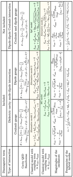
Table S1: Summary of the correspondences between the classical coupled harmonic oscillator models and the cavity-QED Hamiltonians. We consider the coupling between a dipole (representing e.g. a molecular excitation) and a dielectric cavity (with transverse electromagnetic modes) or a plasmonic nanocavity (dipole-dipole coupling via Coulomb interactions). The coupling with transverse modes is described in the Coulomb (second column) and dipole (third column) gauges, while the dipole-dipole coupling is described in the same way in both gauges as indicated in the fourth column. The fourth row shows the cavity-QED Hamiltonians that describe each of these situations. The fifth and the sixth rows indicate the corresponding equations of motion. The fifth mode corresponds to the models associated with coupling terms proportional to oscillator amplitudes, and the sixth row to models with coupling terms proportional to the time derivatives $\dot{x}_{\text{cav}}$ and $\dot{x}_{\text{mat}}$ (with coupling strengths $g_{\scriptscriptstyle{\text{MC}}}$ given by Eq. (S9) and $g_{\scriptscriptstyle{\text{SpC}}}$ given by Eq. (S11)). We highlight in green the SpC and MC models, which are the focus of the main text and for which the frequencies $\omega_{\text{cav}}$ and $\omega_{\text{mat}}$ are considered. We indicate with the yellow background the alternative models where we use renormalized frequencies, which also changes the coupling term. The seventh row includes the association between the amplitudes of the oscillators and physical magnitudes of the system, which is different for the models in the fifth and in the sixth row. The last row gives the frequencies of the two hybrid modes due to each type of interaction.

We summarize in Table S1 all the classical models discussed in Supplementary Secs. S1 and S2 and the cavity-QED Hamiltonians discussed in Supplementary Sec. S3. The models and Hamiltonians included are not limited to those discussed in the main text. Sections S1 and S2 have been focused on two types of interactions: the coupling between a molecular excitation with transverse electromagnetic modes, and the dipole-dipole coupling due to the Coulomb interaction. As can be observed from Table S1, the form of the cavity-QED Hamiltonian depends on the chosen gauge (Coulomb or dipole) [3] for the molecule-dielectric cavity system, but the eigenvalues are gauge-independent and thus they only depend on the type of interaction.

We include in Table S1 the discussed equivalent classical models for each type of interaction. In some of these coupled harmonic oscillator models, the coupling term is proportional to the oscillator displacements $x_{\text{cav}}$ and $x_{\text{mat}}$, while in other models the coupling term is proportional to their time derivatives. We show that if the system is described with the frequencies of the uncoupled oscillators $\omega_{\text{cav}}$ and $\omega_{\text{mat}}$, the description of the interaction between transverse cavity modes and matter excitations requires a coupling term proportional to the time derivatives of the oscillator amplitudes (MC model, equivalent to cavity-QED Hamiltonians with diamagnetic term), while the coupling term associated with dipole-dipole interactions is proportional to the oscillator displacements (SpC model, equivalent to cavity-QED Hamiltonians without diamagnetic term). These classical models analyzed in the main text and in Supplementary Sec. S1 are highlighted by green. On the other hand, as discussed in Supplementary Sec. S2, each type of interaction can also be modelled with alternative models where the variable that appears in the coupling term (oscillator displacements or velocities) is modified. We highlight these models in Table S1 by the yellow squares. In these alternative models, a renormalization in one of the oscillator frequencies is needed to maintain their equivalence with their corresponding cavity-QED Hamiltonians. Further, the alternative classical models also require to modify the physical magnitudes that each oscillator represents. However, if the transformation of oscillator amplitudes and frequencies is done appropriately, all models describing the coupling between transverse fields and dipoles lead to identical results, and the same happens for dipole-dipole interactions.

S5 Transformation from individual to collective oscillators in the description of homogeneous materials in Fabry-Pérot cavities

In Sec. 4.3 of the main article, we analyze how classical models of harmonic oscillators describe an ensemble of $N_{\text{mat}}$ molecules introduced in a Fabry-Pérot cavity. Each molecule couples with all the other molecules and also with the transverse modes of the cavity, and all these interactions can be modelled through Eq. (33b) in the main text. In this supplementary section, we show how to describe this system by considering the coupling of each Fabry-Pérot mode with a single collective mode of matter oscillators. Specifically, here we demonstrate how to transform Eq. (33b) in Sec. 4.3, written in terms of harmonic oscillators of individual molecular excitations, into Eq. (34b), which considers collective modes. This derivation can be generalized to other cavities by following the same procedure but using the spatial distribution of the transverse electric field of the corresponding cavity modes.

We assume that the Fabry-Pérot cavity contains perfect mirrors in the planes $z=0$ and $z=L_{\text{cav}}$ ($L_{\text{cav}}$ is the thickness of the cavity), so that the cavity has transverse electric (TE) modes with field distribution

$$\Xi_{n\mathbf{k}_{\parallel}}(\mathbf{r})=\sin\left(\frac{n\pi z}{L_{\text{cav}}}\right)e^{i\mathbf{k}_{\parallel}\cdot\mathbf{r}_{\parallel}}.$$ (S36)

All modes of the cavity are indexed by the integer $n$ and the wavevector in the parallel direction $\mathbf{k}_{\parallel}$, which can be any two-dimensional vector (we consider a discrete set of $\mathbf{k}_{\parallel}$ by assuming that the cavity has long but finite size in the lateral dimensions and using Born-von Karman periodic boundary conditions for Eq. (S36)). We further assume that the direction of the transition dipole moments of the molecules is the same as that of the electric field of the mode (parallel to the mirror planes). As a consequence, the coupling strength between each molecule placed in the position $\mathbf{r}_{i}=(\mathbf{r}_{\parallel,i},z_{i})$ and the $n\mathbf{k}_{\parallel}$ Fabry-Pérot mode is calculated with the expression $g_{\scriptscriptstyle{\text{MC}}}^{(n\mathbf{k}_{\parallel},i)}=\frac{1}{2}\sqrt{\frac{f_{\text{mat}}}{\varepsilon_{0}V_{\text{eff}}}}\Xi_{n\mathbf{k}_{\parallel}}(\mathbf{r}_{i})$ (see discussion of Supplementary Sec. S1 and Eq. (S9)). By introducing the field distribution of Eq. (S36) in the expression of the coupling strength explicitly, the equations of motion of the system (Eq. (33b)) become

$$\ddot{x}_{\text{cav},n\mathbf{k}_{\parallel}}+\omega^{2}_{\text{cav},n\mathbf{k}_{\parallel}}x_{\text{cav},n\mathbf{k}_{\parallel}}-\sum_{i}\sqrt{\frac{f_{\text{mat}}}{\varepsilon_{0}V_{\text{eff}}}}\sin\left(\frac{n\pi z_{i}}{L_{\text{cav}}}\right)e^{-i\mathbf{k}_{\parallel}\cdot\mathbf{r}_{\parallel i}}\dot{x}_{\text{mat},i}=0,$$ (S37a)

$$\ddot{x}_{\text{mat},i}+\omega^{2}_{\text{mat}}x_{\text{mat},i}+\sum_{n^{\prime},\mathbf{k^{\prime}}_{\parallel}}\sqrt{\frac{f_{\text{mat}}}{\varepsilon_{0}V_{\text{eff}}}}\sin\left(\frac{n^{\prime}\pi z_{i}}{L_{\text{cav}}}\right)e^{i\mathbf{k^{\prime}}_{\parallel}\cdot\mathbf{r}_{\parallel i}}\dot{x}_{\text{cav},n^{\prime}\mathbf{k^{\prime}}_{\parallel}}+\sum_{j\neq i}2\omega_{\text{mat}}g_{\scriptscriptstyle{\text{SpC}}}^{(i,j)}x_{\text{mat},j}=0.$$ (S37b)

In Eq. (S37a), we already observe that the oscillator $x_{\text{cav},n\mathbf{k}_{\parallel}}$ of the $n\mathbf{k}_{\parallel}$ cavity mode is coupled to a collective matter operator. By defining the collective oscillator of the $n\mathbf{k}_{\parallel}$ matter mode as

$$x_{\text{mat},n\mathbf{k}_{\parallel}}=\frac{1}{\sqrt{N_{\text{eff}}}}\sum_{i}e^{-i\mathbf{k}_{\parallel}\cdot\mathbf{r}_{\parallel i}}\sin\left(\frac{n\pi z_{i}}{L_{\text{cav}}}\right)x_{\text{mat},i},$$ (S38)

Equation (S37a) becomes

$$\ddot{x}_{\text{cav},n\mathbf{k}_{\parallel}}+\omega^{2}_{\text{cav},n\mathbf{k}_{\parallel}}x_{\text{cav},n\mathbf{k}_{\parallel}}-\sqrt{N_{\text{eff}}}\overline{g_{\scriptscriptstyle{\text{MC}}}}\dot{x}_{\text{mat},n\mathbf{k}_{\parallel}}=0.$$ (S39)

where $\overline{g_{\scriptscriptstyle{\text{MC}}}}=\frac{1}{2}\sqrt{\frac{f_{\text{mat}}}{\varepsilon_{0}V_{\text{eff}}}}$ is the maximum achievable coupling strength in this system between a single molecule and a cavity mode, for molecules placed in the antinodes of the mode. As discussed below, $N_{\text{eff}}=\sum_{i}|\Xi_{n\mathbf{k_{\parallel}}}(\mathbf{r}_{i})|^{2}$ is the effective number of molecules that couple with the cavity mode, whose exact relation with the total number of molecules $N_{\text{mat}}$ depends on the system and the spatial distribution of the modes. Further, we observe in Eq. (S39) that the coupling strength between the cavity mode and the collective oscillator mode increases as $\overline{g_{\scriptscriptstyle{\text{MC}}}}\sqrt{N_{\text{eff}}}$. This scaling of the coupling strength (together with the scaling as $1/\sqrt{N_{\text{eff}}}$ of the collective oscillator in Eq. (S38)) is the same as in the quantum Dicke model [4], showing that the classical oscillator models are consistent with descriptions based on cavity QED.

The next step is to transform Eq. (S37b), which requires considering $N_{\text{mat}}$ equations simultaneously, one per molecule at position $\mathbf{r}_{i}$. To do the transformation, we multiply Eq. (S37b) by $\frac{1}{\sqrt{N_{\text{eff}}}}\sin\left(\frac{n\pi z_{i}}{L_{\text{cav}}}\right)e^{-i\mathbf{k}_{\parallel}\cdot\mathbf{r}_{\parallel i}}$ for each $i$ molecule and sum the $N_{\text{mat}}$ resulting terms. With this procedure, the transformation of the first two terms is straightforward as

$$\frac{1}{\sqrt{N_{\text{eff}}}}\sum_{i}\sin\left(\frac{n\pi z_{i}}{L_{\text{cav}}}\right)e^{-i\mathbf{k}_{\parallel}\cdot\mathbf{r}_{\parallel i}}(\ddot{x}_{\text{mat},i}+\omega^{2}_{\text{mat}}x_{\text{mat},i})=\ddot{x}_{\text{mat},n\mathbf{k}_{\parallel}}+\omega_{\text{mat}}^{2}x_{\text{mat},n\mathbf{k}_{\parallel}}.$$ (S40)

Repeating the procedure with the third term of Eq. (S37b), we obtain

$$\frac{1}{\sqrt{N_{\text{eff}}}}\overline{g_{\scriptscriptstyle{\text{MC}}}}\sum_{n^{\prime},\mathbf{k^{\prime}}_{\parallel}}\dot{x}_{\text{cav},n^{\prime}\mathbf{k^{\prime}}_{\parallel}}\sum_{i}\sin\left(\frac{n^{\prime}\pi z_{i}}{L_{\text{cav}}}\right)\sin\left(\frac{n\pi z_{i}}{L_{\text{cav}}}\right)e^{i(\mathbf{k}_{\parallel}-\mathbf{k^{\prime}}_{\parallel})\cdot\mathbf{r_{\parallel}}}$$

$$\qquad=\frac{1}{\sqrt{N_{\text{eff}}}}\overline{g_{\scriptscriptstyle{\text{MC}}}}\sum_{n^{\prime},\mathbf{k^{\prime}}_{\parallel}}\dot{x}_{\text{cav},n\mathbf{k}_{\parallel}}\frac{N_{\text{mat}}}{2}\delta_{n,n^{\prime}}\delta_{\mathbf{k}_{\parallel},\mathbf{k^{\prime}}_{\parallel}}=\overline{g_{\scriptscriptstyle{\text{MC}}}}\frac{N_{\text{mat}}}{2}\frac{1}{\sqrt{N_{\text{eff}}}}\dot{x}_{\text{cav},n\mathbf{k}_{\parallel}}.$$ (S41)

Equation (S41) shows that, although each molecule couples with all Fabry-Pérot modes, the collective matter oscillator of amplitude $x_{\text{mat},n\mathbf{k}_{\parallel}}$, described by the indexes $n$ and $\mathbf{k_{\parallel}}$, only couples with the cavity mode of same indexes due to the orthogonality of all these modes. Further, the coupling strength between the cavity mode and the collective matter mode, which is the term multiplying $\dot{x}_{\text{cav},n\mathbf{k}_{\parallel}}$ in Eq. (S41), must be equal to the coupling strength that multiplies $\dot{x}_{\text{mat},n\mathbf{k}_{\parallel}}$ in Eq. (S39). This equality implies that $N_{\text{eff}}=\sum_{i}|\Xi_{n\mathbf{k_{\parallel}}}(\mathbf{r}_{i})|^{2}=N_{\text{mat}}/2$ for the Fabry-Pérot cavity.

Last, we transform the fourth term of Eq. (S37b), which involves molecule-molecule interactions. To perform this transformation, we consider the SpC coupling strength between molecules as given by Eq. (S11) explicitly, which leads to

$$\frac{1}{\sqrt{N_{\text{eff}}}}\sum_{i}\sum_{j\neq i}2\omega_{\text{mat}}g_{\scriptscriptstyle{\text{SpC}}}^{(i,j)}\sin\left(\frac{n\pi z_{i}}{L_{\text{cav}}}\right)e^{-i\mathbf{k}_{\parallel}\cdot\mathbf{r}_{\parallel i}}x_{\text{mat},j}$$

$$=\frac{1}{\sqrt{N_{\text{eff}}}}\sum_{j}2\omega_{\text{mat}}x_{\text{mat},j}e^{-i\mathbf{k}_{\parallel}\cdot\mathbf{r}_{\parallel j}}\sum_{i\neq j}g_{\scriptscriptstyle{\text{SpC}}}^{(i,j)}\sin\left(\frac{n\pi z_{i}}{L_{\text{cav}}}\right)e^{-i\mathbf{k}_{\parallel}\cdot(\mathbf{r}_{\parallel i}-\mathbf{r}_{\parallel j})}$$

$$=\frac{1}{\sqrt{N_{\text{eff}}}}\sum_{j}2\omega_{\text{mat}}x_{\text{mat},j}e^{-i\mathbf{k}_{\parallel}\cdot\mathbf{r}_{\parallel j}}\sum_{i\neq j}\frac{1}{2}\frac{f_{\text{mat}}e^{-i\mathbf{k}_{\parallel}\cdot(\mathbf{r}_{\parallel i}-\mathbf{r}_{\parallel j})}}{4\pi\varepsilon_{0}|\mathbf{r}_{i}-\mathbf{r}_{j}|^{3}\omega_{\text{mat}}}[1-3(\mathbf{n}_{\mathbf{d}}\cdot\mathbf{n}_{\mathbf{r}ij})]\sin\left(\frac{n\pi z_{i}}{L_{\text{cav}}}\right)$$

$$\approx\frac{1}{\sqrt{N_{\text{eff}}}}\sum_{j}2\omega_{\text{mat}}x_{\text{mat},j}e^{-i\mathbf{k}_{\parallel}\cdot\mathbf{r}_{\parallel j}}\sin\left(\frac{n\pi z_{j}}{L_{\text{cav}}}\right)\underbrace{\sum_{i\neq j}\frac{1}{2}\frac{f_{\text{mat}}e^{-i\mathbf{k}_{\parallel}\cdot(\mathbf{r}_{\parallel i}-\mathbf{r}_{\parallel j})}}{4\pi\varepsilon_{0}|\mathbf{r}_{i}-\mathbf{r}_{j}|^{3}\omega_{\text{mat}}}[1-3(\mathbf{n}_{\mathbf{d}}\cdot\mathbf{n}_{\mathbf{r}ij})]}_{\overline{g_{\scriptscriptstyle{\text{SpC}}}^{(n\mathbf{k}_{\parallel})}}}$$ (S42)

$$\qquad=2\omega_{\text{mat}}\overline{g_{\scriptscriptstyle{\text{SpC}}}^{(n\mathbf{k}_{\parallel})}}x_{\text{mat},n\mathbf{k}_{\parallel}}.$$ (S43)

To obtain Eq. (S42), we have considered that the dipole-dipole coupling strength between different molecules, which depends over their distance as $|\mathbf{r}_{i}-\mathbf{r}_{j}|^{-3}$, decays much faster over $z$ than the term $\sin(n\pi z/L_{\text{cav}})$ changes (unless $n$ is so large that it has very fast oscillations, which we do not consider here). Due to this fast decay, we have checked numerically that the term $\sin(n\pi z/L_{\text{cav}})$ can be taken outside the sum over molecules $i$ as a constant. The sum over the variable $i$ in Eq. (S42) can be then performed numerically to obtain the collective molecule-molecule coupling strength $\overline{g_{\scriptscriptstyle{\text{SpC}}}^{(n\mathbf{k}_{\parallel})}}$.

Therefore, by gathering all transformed terms in Eqs. (S40), (S41) and (S43), Eq. (S37b) becomes

$$\ddot{x}_{\text{mat},n\mathbf{k}_{\parallel}}+(\omega_{\text{mat}}^{2}+2\omega_{\text{mat}}\overline{g_{\scriptscriptstyle{\text{SpC}}}^{(n\mathbf{k}_{\parallel})}})x_{\text{mat},n\mathbf{k}_{\parallel}}+\overline{g_{\scriptscriptstyle{\text{MC}}}}\sqrt{N_{\text{eff}}}\dot{x}_{\text{cav},n\mathbf{k}_{\parallel}}=0.$$ (S44)

Equations (S39) and (S44) correspond to Eq. (34b) in the main article. Importantly, the derivation carried out in this section shows two important features of light-matter coupling in this system: i) although each $n\mathbf{k}_{\parallel}$ cavity mode is coupled to all individual molecules, it is only coupled to the $n\mathbf{k}_{\parallel}$ collective mode due to the orthogonality of the modes, and ii) the only consequence of the molecule-molecule coupling for the interaction between the $n\mathbf{k}_{\parallel}$ cavity and matter modes is to renormalize the bare frequency of the matter oscillator from $\omega_{\text{mat}}$ to $\sqrt{\omega_{\text{mat}}^{2}+2\omega_{\text{mat}}\overline{g_{\scriptscriptstyle{\text{SpC}}}^{(n\mathbf{k}_{\parallel})}}}$ [5].

References

- [1] P. Törmä and W. L. Barnes, Strong coupling between surface plasmon polaritons and emitters: a review. Rep. Prog. Phys. 78, 013901 (2015).
- [2] D. S. Dovzhenko, S. V. Ryabchuk, Y. P. Rakovich, and I. R. Nabiev, Light–matter interaction in the strong coupling regime: configurations, conditions, and applications. Nanoscale 10, 3589-3605 (2018).
- [3] J. M. Fink et al., Climbing the Jaynes-Cummings ladder and observing its nonlinearity in a cavity QED system. Nature 454, 315-318 (2008).
- [4] R. Sáez-Blázquez, J. Feist, A. I. Fernández-Domínguez, and F. J. García-Vidal, Enhancing photon correlations through plasmonic strong coupling. Optica 4, 1363-1367 (2017).
- [5] A. Thomas et al., Tilting a ground-state reactivity landscape by vibrational strong coupling. Science 363, 615-619 (2019).
- [6] E. Orgiu et al., Conductivity in organic semiconductors hybridized with the vacuum field. Nat. Mater. 14, 1123-1129 (2015).
- [7] G. Rempe and H. Walther, Observation of quantum collapse and revival in a one-atom maser. Phys. Rev. Lett. 58, 353 (1987).
- [8] R. J. Thompson, G. Rempe, and H. J. Kimble, Observation of normal-mode splitting for an atom in an optical cavity. Phys. Rev. Lett. 68, 1132 (1992).
- [9] Y. Kaluzny, P. Goy, M. Gross, J. M. Raimond, and S. Haroche, Observation of self-induced Rabi oscillations in two-level atoms excited inside a resonant cavity: the ringing regime of superradiance. Phys. Rev. Lett. 51, 1175 (1983).
- [10] M. Brune, J. M. Raimond, P. Goy, L. Davidovich, and S. Haroche, Realization of a two-photon maser oscillator. Phys. Rev. Lett. 59, 1899 (1987).
- [11] M. G. Raizen, R. J. Thompson, R. J. Brecha, H. J. Kimble, and H. J. Carmichael, Normal-mode splitting and linewidth averaging for two-state atoms in an optical cavity. Phys. Rev. Lett. 63, 240 (1989).
- [12] J. P. Reithmaier et al., Strong coupling in a single quantum dot-semiconductor microcavity system. Nature 432, 197-200 (2004).
- [13] S. Christopoulos et al., Room-temperature polariton lasing in semiconductor microcavities. Phys. Rev. Lett. 98, 126405 (2007).
- [14] A. Wallraff et al., Strong coupling of a single photon to a superconducting qubit using circuit quantum electrodynamics. Nature 431, 162-167 (2004).
- [15] T. K. Hakala et al., Vacuum Rabi splitting and strong-coupling dynamics for surface-plasmon polaritons and rhodamine 6G molecules. Phys. Rev. Lett. 103, 053602 (2009).
- [16] P. Vasa et al., Ultrafast manipulation of strong coupling in metal-molecular aggregate hybrid nanostructures. ACS Nano 4, 7559–7565 (2010).
- [17] R. Chikkaraddy et al., Single-molecule strong coupling at room temperature in plasmonic nanocavities. Nature 535, 127-130 (2016).
- [18] J. Feist, J. Galego, and F. J. García-Vidal, Polaritonic chemistry with organic molecules. ACS Photonics 5, 205-216 (2018).
- [19] T. Niemczyk et al., Circuit quantum electrodynamics in the ultrastrong-coupling regime. Nat. Phys. 2, 81-90 (2006).
- [20] A. F. Kockum, A. Miranowicz, S. De Liberato, S. Savasta, and F. Nori, Ultrastrong coupling between light and matter. Nat. Rev. Phys. 1 19-40 (2019).
- [21] P. Forn-Díaz, L. Lamata, E. Rico, J. Kono, and E. Solano, Ultrastrong coupling regimes of light-matter interaction. Rev. Mod. Phys. 91, 025005 (2019).
- [22] C. Ciuti, G. Bastard, and I. Carusotto, Quantum vacuum properties of the intersubband polariton field. Phys. Rev. B. 72, 115303 (2005).
- [23] K. Rzazewski, K. Wodkiewicz, and W. Zakowicz, Phase transitions, two-level atoms and the term. Phys. Rev. Lett. 35, 432 (1975).
- [24] P. Nataf and C. Ciuti, No-go theorem for superradiant quantum phase transitions in cavity QED and counter-example in circuit QED. Nat. Commun. 1, 72 (2010).
- [25] A. Vukics and P. Domokos, Adequacy of the Dicke model in cavity QED: A counter-no-go statement. Phys. Rev. A 86, 053807 (2012).
- [26] T. Tufarelli, K. R. McEnergy, S. A. Maier, and M. S. Kim, Signatures of the term in ultrastrongly coupled oscillators. Phys. Rev. A 91, 063840 (2015).
- [27] D. De Bernardis, T. Jaako, and P. Rabl, Cavity quantum electrodynamics in the nonperturbative regime. Phys. Rev. A 97, 043820 (2018).
- [28] C. Schäfer, M. Ruggenthaler, V. Rokaj, and A. Rubio, Relevance of the quadratic diamagnetic and self-polarization terms in cavity quantum electrodynamics. ACS Photonics 7, 975-990 (2020).
- [29] J. Galego, C. Climent, F. J. Garcia-Vidal, and J. Feist, Cavity Casimir-Polder Forces and Their Effects in Ground-State Chemical Reactivity. Phys. Rev. X 9, 021057 (2019).
- [30] J. Feist, A. I. Fernández-Domínguez, and F. J. García-Vidal, Macroscopic QED for quantum nanophotonics: emitter-centered modes as a minimal basis for multiemitter problems. Nanophotonics 10, 477-489 (2021).
- [31] L. Novotny, Strong coupling, energy splitting, and level crossings: a classical perspective. Am. J. Phys. 78 1199-1202 (2010).
- [32] S. R. K. Rodriguez, Classical and quantum distinctions between weak and strong coupling. Eur. J. Phys. 37 025802 (2016).
- [33] S. Rudin and T. L. Reinecke, Oscillator model for vacuum Rabi splitting in microcavities. Phys. Rev. B 59 10227 (1999).
- [34] A. B. Lockhart, A. Skinner, W. Newman, D. B. Steinwachs, and S. A. Hilbert, An experimental demonstration of avoided crossings with masses on springs. Am. J. Phys. 86, 526 (2018).
- [35] Y. S. Joe, A. M. Satanin, and C. S. Kim, Classical analogy of Fano resonances. Phys. Scr. 74, 259 (2006).
- [36] P. D. Hemmer and M. G. Prentiss, Coupled-pendulum model of the stimulated resonance Raman effect. J. Opt. Soc. Am. B 5, 1613-1623 (1988).
- [37] C. L. Garrido Alzar, M. A. G. Martinez, and P. Nussenzveig, Classical analog of electromagnetically induced transparency. Am. J. Phys. 70, 37-41 (2002).
- [38] J. Harden, A. Joshi, and J. D. Serna, Demonstration of double EIT using coupled harmonic oscillators and RLC circuits. Eur. J. Phys 32 541-558 (2011).
- [39] J. A. Souza, L. Cabral, R. R. Oliveira, and C. J. Villas-Boas, Electromagnetically-induced-transparency-related phenomena and their mechanical analogs. Phys. Rev. A 92, 023818 (2015).
- [40] M. Harder and C.-M. Hu, Cavity spintronics: an early review of recent progress in the study of magnon-photon level repulsion. Solid State Phys. 69, 47–121 (2018).
- [41] X. Liu et al., Strong light-matter coupling in two-dimensional atomic crystals. Nat. Photonics 9, 30-34 (2015).
- [42] D. Yoo et al., Ultrastrong plasmon-phonon coupling via epsilon-near-zero nanocavities. Nat. Photonics 15, 125-130 (2021).
- [43] J. George et al., Multiple Rabi Splittings under Ultrastrong Vibrational Coupling. Phys. Rev. Lett. 117, 153601 (2016).
- [44] K. Nagarajan, A. Thomas, and T. W. Ebbesen, Chemistry under Vibrational Strong Coupling. J. Am. Chem. Soc. 143, 16877 (2021).
- [45] C. Symonds et al., Particularities of surface plasmon-exciton strong coupling with large Rabi splitting. New J. Phys. 10 065017 (2008).
- [46] S. Wang et al., Coherent coupling of WS2 monolayers with metallic photonic nanostructures at room temperature. Nano Lett. 16, 4368-4374 (2016).
- [47] D. Zheng, S. Zhang, Q. Deng, M. Kang, P. Nordlander, and H. Xu, Manipulating coherent plasmon-exciton interaction in a single silver nanorod on monolayer WSe2. Nano Lett. 17, 3809-3814 (2017).
- [48] M. Stührenberg et al., Strong light-matter coupling between plasmons in individual gold bi-pyramids and excitons in mono- and multilayer WSe2. Nano Lett. 18, 5938-5945 (2018).
- [49] M. Autore et al., Boron nitride nanoresonators for phonon-enhanced molecular vibrational spectroscopy at the strong coupling limit. Light: Science applications. 7, 17172 (2018).
- [50] N. Liu et al., Plasmonic analogue of electromagnetically induced transparency at the Drude damping limit. Nature Mater. 8, 758–762 (2009).
- [51] X. Wu, S. K. Gray, and M. Pelton, Quantum-dot-induced transparency in a nanoscale plasmonic resonator. Opt. Express 18, 23633–23645 (2010).
- [52] S. R. K. Rodriguez, Y. T. Chen, T. P. Steinbusch, M. A. Verschuuren, A. F. Koenderink, J. Gómez Rivas, From weak to strong coupling of localized surface plasmons to guided modes in a luminescent slab. Phys. Rev. B 90, 235406 (2014).
- [53] M. Barra-Burillo, U. Muniain et al., Microcavity phonon polaritons from the weak to the ultrastrong phonon-photon coupling regime. Nat. Commun. 12, 6206 (2021).
- [54] G. Khitrova, H. M. Gibbs, M. Kira, S. W. Koch, and A. Scherer, Vacuum Rabi splitting in semiconductors. Nat. Phys. 2, 81-90 (2006).
- [55] H. Bellessa, C. Bonnand, J. C. Plenet, and J. Mugnier, Strong coupling between surface plasmon and excitons in an organic semiconductor. Phys. Rev. Lett. 93, 036404 (2004).
- [56] J. J. Hopfield, Theory of the contribution of excitons to the complex dielectric constant of crystals. Phys. Rev. 112, 1555 (1958).
- [57] E. M. Purcell, Spontaneous emission probabilities at radio frequencies. Phys. Rev. 69, 681 (1946).
- [58] M. Pelton, Modified spontaneous emission in nanophotonic structures. Nat. Photonics 9, 427–435 (2015)
- [59] J. McKeever, A. Boca, A. D. Boozer, J. R. Buck, and H. J. Kimble, Experimental realization of a one-atom laser in the regime of strong coupling. Nature 425, 268–271 (2003).
- [60] R. Sáez-Blázquez, J. Feist, F. J. García-Vidal, and A. I. Fernández-Domínguez, Photon statistics in collective strong coupling: Nanocavities and microcavities. Phys. Rev. A 98, 013839 (2018).
- [61] Á. Nodar, R. Esteban, U. Muniain, M. J. Steel, J. Aizpurua, and M. K. Schmidt, Identifying unbound strong bunching and the breakdown of the Rotating Wave Approximation in the quantum Rabi model. Phys. Rev. Research 5, 043213 (2023).
- [62] M. Thorwart, L. Hartmann, I. Goychuk, and P. Hänggi, Controlling decoherence of a two-level atom in a lossy cavity. J. Mod. Opt. 47, 2905–2919 (2000).
- [63] C. Cohen-Tannoudji, J. Dupont-Roc, and G. Grynberg, Photons and Atoms (Wiley, New York, 1997).
- [64] R. Esteban, J. Aizpurua, and G. W. Bryant, Strong coupling of single emitters interacting with phononic infrared antennae. New J. Phys 16, 013052 (2014).
- [65] J. S. Foresi et al., Photonic-bandgap microcavities in optical waveguides. Nature 390, 143-145 (1997).
- [66] M. Kuisma et al., Ultrastrong coupling of a single molecule to a plasmonic nanocavity: a first-principles study. ACS Photonics 9, 1065-1077 (2022).
- [67] M. Pelton, S. D. Storm, and H. Leng, Strong coupling of emitters to single plasmonic nanoparticles: exciton-induced transparency and Rabi splitting. Nanoscale 11, 14540 (2019).
- [68] E. Waks and D. Sridharan, Cavity QED treatment of interactions between a metal nanoparticle and a dipole emitter. Phys. Rev. A 82, 043845 (2010).
- [69] A. Trügler and U. Hohenester, Strong coupling between a metallic nanoparticle and a single molecule. Phys. Rev. B 77, 115403 (2008).
- [70] W. L. Barnes, Particle plasmons: why shape matters. Am. J. Phys 84, 593-601 (2016).
- [71] C. C. Gerry and P. L. Knight, Introductory Quantum Optics (Cambridge University Press, 2004).
- [72] L. Novotny and B. Hecht, Principles of Nano-Optics (Cambridge University Press, 2006).
- [73] A. Delga, J. Feist, J. Bravo-Abad, and F. J. García-Vidal, Quantum emitters near a metal nanoparticle: strong coupling and quenching. Phys. Rev. Lett. 112, 253601 (2014).
- [74] S. Kéna-Cohen, S. A. Maier, and D. C. D. Bradley, Ultrastrongly coupled exciton–polaritons in metal-clad organic semiconductor microcavities. Adv. Optical Mater. 1, 827–833 (2013).
- [75] S. Brodbeck et al., Experimental Verification of the Very Strong Coupling Regime in a GaAs Quantum Well Microcavity. Phys. Rev. Lett. 119, 027401 (2017).
- [76] R. H. Dicke, Coherence in spontaneous radiation processes. Phys. Rev. 93, 99 (1954).
- [77] T. Schwartz, J. A. Hutchison, C. Genet, and T. W. Ebbesen, Reversible switching of ultrastrong light-molecule coupling. Phys. Rev. Lett. 106, 196405 (2011).
- [78] F. Barachati et al., Tunable third-harmonic generation from polaritons in the ultrastrong coupling regime. ACS Photonics 5, 119–125 (2018).
- [79] S. Ribeiro, J. Aizpurua, and R. Esteban, Influence of direct dipole-dipole interactions on the optical response of two-dimensional materials in strongly inhomogeneous infrared cavity fields. Phys. Rev. A 108, 043718 (2023).
- [80] A. Canales, D. G. Baranov, T. J. Antosiewicz, and T. Shegai, Abundance of cavity-free polaritonic states in resonant materials and nanostructures. J. Chem. Phys. 154, 024701 (2021).
- [81] D. R. Abujetas, J. Feist, F. J. García-Vidal, J. Gómez Rivas, and J. A. Sánchez-Gil, Strong coupling between weakly guided semiconductor nanowire modes and an organic dye. Phys. Rev. B 99, 205409 (2019).
- [82] N. W. Ashcroft and N. D. Mermin, Solid state physics (Saunders College Publishing, 1976).
- [83] T. Holstein and H. Primakoff, Field dependence of the intrinsic domain magnetization of a ferromagnet. Phys. Rev. 58, 1098 (1940).
Supplementary Information for:
Description of ultrastrong light-matter interaction through coupled harmonic oscillator models and their connection with cavity-QED Hamiltonians
Unai Muniain1, Javier Aizpurua1,2,3, Rainer Hillenbrand2,3,4, Luis Martín-Moreno5,6 and Ruben Esteban1,7
1Donostia International Physics Center, Paseo Manuel de Lardizabal 4, 20018 Donostia-San Sebastián, Spain
2IKERBASQUE, Basque Foundation for Science, María Díaz de Haro 3, 48013 Bilbao, Spain
3Department of Electricity and Electronics, University of the Basque Country (UPV/EHU), 48940 Leioa, Spain
4CIC nanoGUNE BRTA, Tolosa Hiribidea 76, 20018 Donostia-San Sebastián, Spain
5Departamento de Física de la Materia Condensada, Universidad de Zaragoza, 50009 Zaragoza, Spain
6Instituto de Nanociencia y Materiales de Aragón (INMA), CSIC-Universidadd de Zaragoza, 50009 Zaragoza, Spain
7Materials Physics Center, CSIC-UPV/EHU, Paseo Manuel de Lardizabal 5, 20018 Donostia-San Sebastián, Spain

References

- [1] C. Cohen-Tannoudji, J. Dupont-Roc, and G. Grynberg, Photons and Atoms (Wiley, New York, 1997).
- [2] R. Guy Woolley, Power-Zienau-Woolley representations of nonrelativistic QED for atoms and molecules. Phys. Rev. Research 2, 013206 (2020).
- [3] D. L. Andrews, G. A. Jones, A. Salam, and R. Guy Woolley, Perspective: Quantum Hamiltonians for optical interactions. J. Chem. Phys. 148 040901 (2018).
- [4] R. H. Dicke, Coherence in spontaneous radiation processes. Phys. Rev. 93, 99 (1954).
- [5] S. Ribeiro, J. Aizpurua, and R. Esteban, Influence of direct dipole-dipole interactions on the optical response of two-dimensional materials in strongly inhomogeneous infrared cavity fields. Phys. Rev. A 108, 043718 (2023).