Stylized Facts of High-Frequency Bitcoin Time Series

Abstract

This paper analyses the high-frequency intraday Bitcoin dataset from 2019 to 2022. During this time frame, the Bitcoin market index exhibited two distinct periods characterized by abrupt changes in volatility. The Bitcoin price returns for both periods can be described by an anomalous diffusion process, transitioning from subdiffusion for short intervals to weak superdiffusion over longer time intervals. The characteristic features related to this anomalous behavior studied in the present paper include heavy tails, which can be described using a $q$-Gaussian distribution and correlations. When we sample the autocorrelation of absolute returns, we observe a power-law relationship, indicating time dependency in both periods initially. The ensemble autocorrelation of returns decays rapidly and exhibits periodicity. We fitted the autocorrelation with a power law and a cosine function to capture both the decay and the fluctuation and found that the two periods have distinctive periodicity. Further study involves the analysis of endogenous effects within the Bitcoin time series, which are examined through detrending analysis. We found that both periods are multifractal and present self-similarity in the detrended probability density function (PDF). The Hurst exponent over short time intervals shifts from less than 0.5 ($\sim$ 0.42) in Period 1 to be closer to 0.5 in Period 2 ($\sim$ 0.49), indicating the market is more efficient at short time scales.

I Introduction

Cryptocurrencies offer a decentralized and innovative alternative to traditional financial systems Corbet et al. (2019). Despite not being globally accepted as digital currency, many consider cryptocurrencies valuable assets for storing and retrieving value when needed Crosby et al. (2016). With over 2,000 distinct cryptocurrencies currently in circulation, their potential and prominence continue growing Noam (2021). In this dynamically evolving market, Bitcoin stands out as the dominant one. Introduced by Nakamoto Nakamoto (2008) in 2008 as the first decentralized cryptocurrency, Bitcoin has witnessed a substantial increase in its market value. Statistics from CoinMarketCap reveal that Bitcoin’s market capitalization reached 567.61 billion USD as of August 3, 2023, constituting 48.09% of the aggregate market capitalization of major cryptoassets Coi (2023). Bitcoin operates as an open accessible network, providing an emerging market free from the constraints of traditional trading hours. It captures the attention of practitioners, individuals who see value in associating Bitcoin with their addresses on the blockchain, and academics intrigued by its durability and the broader understanding of blockchain-based cryptocurrencies.

Bitcoin was created as an online payment system that enables users to engage in direct transactions without intermediaries Nakamoto (2008). Its decentralized nature ensures independence from central banks or government authorities responsible for currency issuance Underwood (2016); Zaghloul et al. (2020). The adoption of Bitcoin for payments of goods and services has experienced substantial growth. Some argue that businesses find it advantageous to accept Bitcoin, citing lower transaction fees compared to the typical 2-3% imposed by credit card processors Hong (2017). Conversely, investors perceive Bitcoin as an alternative investment avenue, as indicated by an analysis of transactions from 2011 to 2014 Baur et al. (2015). Bitcoin has sometimes been referred to as the ‘digital gold’ Popper (2016), attracting individual investors seeking portfolio diversification as a replacement for gold as a hedge against inflation Henriques and Sadorsky (2018). This investment interest extends beyond individual investors to various institutional players, including the Global Advisors Bitcoin Investment Fund, Pantera Capital, and Falcon Global Capital, which initiated Bitcoin investments as early as 2013 Hong (2017). Various types of institutions that hold Bitcoin have emerged, including the Bitcoin Exchange-Traded Funds (ETFs) that track the value of Bitcoin. These ETFs attract investors and speculators by facilitating transactions through traditional stock market exchanges rather than cryptocurrency trading platforms. Presently, a significant portion of Bitcoin is under institutional ownership, ranging from ETFs to sovereign governments like El Salvador Genç (2023). Institutional investment in Bitcoin takes various forms, encompassing direct ownership, participation in mining companies, Bitcoin futures ETFs, or integration into retirement strategies Genç (2023).

The peer-to-peer characteristic of Bitcoin is underpinned by blockchain technology, which functions as a shared public ledger of all transactions and digital events among participants Underwood (2016); Crosby et al. (2016); Zaghloul et al. (2020). This technology has demonstrated its versatility by finding applications in both financial and non-financial domains. Financial institutions and banks actively explore innovative blockchain applications, with a focus on areas such as private securities and insurance Crosby et al. (2016). A notable example is Decentralized Finance (DeFi), which represents a groundbreaking financial paradigm built on blockchain, providing services like loans, insurance, and financial assets exchange without reliance on a central authority Auer et al. (2023). DeFi is gaining attention from investment banks and central banks, with initiated programs to explore the potential applications of digital assets Genç (2023). The non-financial applications of blockchain technology also hold considerable promise. Serving as a decentralized storage system, blockchain facilitates the storage of various file types. This technology can verify the existence of diverse documents, including legal documents, health records, loyalty payments, and licenses across various industries. By storing the fingerprint of the asset instead of the asset itself, blockchain ensures enhanced privacy and anonymity Crosby et al. (2016).

With an increasing number of users adopting Bitcoin, and despite its meaningful fluctuations, high volatility, and dependence on evolving technology, this emerging asset continues to gain importance in our economy. Previous studies have extensively explored various aspects of Bitcoin, including its market efficiency Urquhart (2016); Kurihara and Fukushima (2017); Jiang et al. (2018); Caporale et al. (2018); Noda (2021); Bariviera et al. (2017); Mnif et al. (2020); Mnif and Jarboui (2021); Fernandes et al. (2022); Montasser et al. (2022); Kakinaka and Umeno (2022), regulatory requirements Brito et al. (2014); Böhme et al. (2015); Hendrickson and Luther (2017); Marian (2013); Gross et al. (2017), market dynamics and its correlations with various asset classes Conrad et al. (2018); Ciaian et al. (2018); Klein et al. (2018); Eross et al. (2019); Ariya et al. (2020); Arias-Calluari et al. (2021); Hu et al. (2019); De Sousa Filho et al. (2021); Cremaschini et al. (2023); Ghosh et al. (2023); Bariviera et al. (2017); De Sousa Filho et al. (2021); Wen et al. (2022); Zhang et al. (2018), with the intent to quantify Bitcoin price fluctuations and evaluate their proximity to stock market prices mechanisms. Given that the Bitcoin pricing mechanism differs from conventional stock market price indexes, we propose initiating the analysis by examining robust patterns or ‘stylized facts’ of Bitcoin price fluctuations. This analysis is based on ‘tick-by-tick’ recorded data from Reuters Datascope. The motivation lies in unveiling precise time-scale properties of Bitcoin time series, allowing comparisons with the widely acknowledged stylized facts from stock market data Cont (2001), e.g. fat tails, volatility clustering, short-time correlations, and self-similarity measurements. To do this we analyze the intraday data of the BTC/USD exchange, spanning the years 2018 to 2022. The dataset has a frequency of 10 minutes, and trading occurs continuously throughout the 24-hour day.

The paper is organized as follows: Section II recalls well-known stylized facts observed in financial time series. Section III presents a background of the Bitcoin cryptocurrency, essential for understanding the dynamics of Bitcoin transactions. In Section IV, we provide the governing equations adapted from our closest model obtained for stock market prices for this study, along with the notations used in this paper. In Section V, we divide the Bitcoin time series into different time periods characterized by the abrupt change in the volatility, and then we examine the stylized facts for each period, respectively. Finally, we provide a summary of our findings based on the comparative analysis of the S&P 500 and Bitcoin.

II Stylized facts of financial markets

For the evaluation of financial models and the development of econometric theories, researchers focus on studying persistent statistical characteristics of the market, commonly referred to as ‘stylized facts’.

Stylized fact is a widely adopted concept in economics, referring to the common statistical properties observed across datasets spanning different timeframes Cont (2001); Chakraborti et al. (2011). The concept of stylized facts, initially introduced in macroeconomics to describe statistical patterns characterizing macroeconomic growth over extended periods and across diverse countries Kaldor (1961), has undergone extensive examination in traditional financial instruments. In stock markets, widely recognized stylized facts include phenomena such as fat-tailed distribution, volatility clustering, self-similarity of market returns, and seasonality in time series Bollerslev et al. (1994); Cont (2001); Chakraborti et al. (2011); Nystrup et al. (2015); Shakeel and Srivastava (2018); Arias-Calluari et al. (2021). Analyzing stylized facts is crucial for establishing the foundation for the development of theoretical forecasting models (Rydén et al. (1998); Liesenfeld and Jung (2000); Andersson (2001); Carnero (2004); Bulla and Bulla (2006); Malmsten and Teräsvirta (2010); Chakraborti et al. (2011)). A substantial body of evidence suggests that cryptocurrency markets exhibit the key stylized characteristics observed in foreign exchange markets Segnon and Bekiros (2020); Bariviera et al. (2017). These findings motivate a careful analysis of the most well-known stylized facts in stock markets before seeking future modeling approaches. In this section, we dedicate ourselves to recalling each of these well-known stylized facts along with their corresponding descriptions, as listed below:

1. fat-tailed distribution of returns: This phenomenon was initially recognized by Mandelbrot Mandelbrot (1963), based on empirical distributions of financial returns (and log-returns) that exhibit heavy-tailed distributions, deviating from the Gaussian distribution Cont (2001); Chakraborti et al. (2011). The presence of heavy tails indicates a higher likelihood of extreme events than predicted by a normal distribution Stoyanov et al. (2011). Within a self-similar fat-tailed distribution, the tails can be characterized by a power law relation denoted as $P(x,t)\sim t^{-H}F(xt^{-H})$, where $P(x,t)$ represents the probability distribution function (PDF) of the price return $x$. $F$ was widely assumed to follow a distribution known as a Levy distribution from the 1990s, $F(x)=L_{\alpha}(x)$, $H=1/\alpha$ where $\alpha\in(0,2]$ Lèvy (1937); Mantegna and Stanley (1994, 1999). After the 2000, $F$ was considered as a q-Gaussian distribution, $F(x)=g_{q}(x)$, $H=1/\alpha$ , where $\alpha=\frac{3-q}{\xi}$ with $q\in(1,3)$ and $\xi$ as a constant parameterBorland and Bouchaud (2004); Queirós (2005); Malamud (2003); Alonso-Marroquin et al. (2019). More recently $F$ is viewed as the solution of a general porous media equation solved through local derivatives $H(t)=1/\alpha(t)$, where $\alpha(t)=\frac{3-q(t)}{\xi(t)}$ Gharari et al. (2021); Tang et al. (2023).

2. short-time autocorrelation of returns: The autocorrelation function (ACF) quantifies the relationship between the current data and historical data, showing the extent to which there is some form of ‘memory’ in the market Vilela et al. (2013); Nounou and Bakshi (2000). The memory is commonly defined as the critic shifted time for the autocorrelation process $\tau_{c}=1/ACF(0)\int_{0}^{\infty}ACF(\tau)d\tau$ Kasdin (1995). In terms of financial data analysis, ACF is evaluated using price returns and describes a rapid decay during very small intraday time scales, before decaying to zero value Cont (2001); Chakraborti et al. (2011). This trend aligns with the efficient market hypothesis De Sousa Filho et al. (2021); Cont (2001), signifying a finite memory; it retains correlation with values closer back in time only.

3. volatility clustering: Volatility in finance measures the extent to which actual returns deviate from average returns over a designated time span Kumar (2016). It is related to the risk management of assets, with higher volatility implying a greater chance of substantial losses De Silva et al. (2017). Volatility is commonly quantified as the standard deviation ($\sigma$) of the returns, and it plays an important role as an estimation tool in empirical investigations in financial studies, especially when examining new and emerging assets Ghosh et al. (2023). Regarding stylized facts, volatility clustering is a widely observed phenomenon, particularly in speculative return time series. Mandelbrot initially identified this pattern Mandelbrot (1963), denoting the tendency for substantial changes to be succeeded by similarly substantial changes, and minor changes to be succeeded by comparably minor changes. This underscores the empirical reality that price fluctuations are non-stationary processes as the fluctuations are not identically distributed and the distributions experience temporal shifts Chakraborti et al. (2011).

4. self-similarity and fractality: Broadly defined, a fractal refers to a geometric shape that exhibits fragmented characteristics, with each fragment (at least approximately) resembling a reduced-scale replica of the whole structure Chen et al. (2016). A fractal can be described by its scale-invariant fractal dimension Mandelbrot and Mandelbrot (1982), which is directly related to the Hurst exponent, $H$. Fractals have been studied extensively in finance and economics, including the stock market Lee et al. (2017), gold Mali and Mukhopadhyay (2014), electricity Wang et al. (2013), crude oil Gu et al. (2010), and shipping markets Chen et al. (2016). In the domains of finance and economics, substantial research has explored the concept of fractals and scaling laws Önalan (2004). Scaling laws establish a connection between price returns computed over various sampling intervals, highlighting that the shape of PDF of price return remains consistent as the time scale varies, $P(x,t)\sim t^{-H}F(xt^{-H})$Gharari et al. (2021), where a self-similar time series denotes $\sqrt{\langle x^{2}\rangle}\propto t^{H}$. Fractal analysis techniques such as rescaled range analysis (R/S) and Detrended Fluctuation Analysis (DFA) have been pivotal in these investigations Lahmiri and Bekiros (2018). Both methods yield a spectrum of Hurst exponent, enabling the determination of the fractality of the time series. However, the R/S statistic is susceptible to outlier influence, potentially leading to a biased estimation of the Hurst exponent Gu et al. (2010). Therefore, in this study, we adopt the multifractal detrended fluctuation analysis (MF-DFA) method, which is a generalization of the DFA, owing to its proficiency in handling nonstationary time series Lahmiri and Bekiros (2018).

Besides these well-acknowledged facts, financial markets exhibit other widely observed statistical characteristics, one of which is the anomalous diffusion in the peak of the PDF of returns. Bachelier’s Bachelier (1900) original work on market fluctuations also introduced the first option pricing model grounded in Brownian motion, associating this motion with price return fluctuations. Later the Black-Scholes equation was proposed to improve the Brownian motion model to prevent the possibility of negative prices Black and Scholes (1973). The Black-Scholes model is alternately referred to as the geometric Brownian model. However, these models fall short of effectively characterizing numerous dynamic processes Weron and Magdziarz (2009). This limitation arises from the fact that the mean squared displacement of the price return scales with time exhibiting a fractional exponent deviating from conventional Brownian motion Sposini et al. (2022a), $H\neq 0.5$ and is not a unique value $H(t)=1/\alpha(t)$; this deviation is known as anomalous diffusion. Anomalous diffusion is widely observed within financial data and is expressible through a power law relation $P_{max}\sim t^{-1/\alpha(t)}$, where $P_{max}$ represents the peak of the PDF of the future price return, and $t$ represents the predicted time Alonso-Marroquin et al. (2019). Here, $\alpha=2$ indicates normal (Brownian) diffusion, $\alpha<2$ implies superdiffusion, and $\alpha>2$ denotes subdiffusion Sposini et al. (2022a). Moreover, the value of $\alpha$ is intricately tied to the Hurst exponent ($H$) through the relation $H=1/\alpha(t)$ Gharari et al. (2021); Sposini et al. (2022a); Ghosh et al. (2023). For example, this relationship is valid in fraction Brownian motion, which is a self-similar Gaussian stochastic process characterized by stationary power-law correlated increments Gharari et al. (2021).

The aforementioned statistical properties are typically observed in traditional markets. This paper seeks to evaluate these properties in the context of Bitcoin, drawing comparisons with conventional markets. Given the distinctive framework of Bitcoin compared to traditional markets, the following section will offer a brief overview of its characteristics.

III Bitcoin’s Operational Framework

Cryptocurrencies are decentralized digital assets that rely on encryption to verify transactions. Bitcoin, being the first, largest, and most well-known cryptocurrency, operates differently from centralized money systems. For centralized money, currency is issued by central banks and transactions involve intermediaries like banks. In contrast, Bitcoin employs a decentralized digital infrastructure called “blockchain” for peer-to-peer transactions and value storage. This allows Bitcoin to operate independently of any government, company, or financial institution. The concept of blockchain was initially proposed in 1991 Haber and Stornetta (1991) and further developed by Satoshi Nakamoto Nakamoto (2008). A blockchain is a public ledger of all transactions and digital events shared among participating parties since the creation of Bitcoin Underwood (2016); Crosby et al. (2016). The blockchain maintains a certain and verifiable record of every single transaction and ownership and once lodged, the transaction can never be erased Crosby et al. (2016); Vujičić et al. (2018). Additionally, blockchain technology prevents double-spending, enhancing the security level of Bitcoin cryptocurrency Kuo Chuen et al. (2018). This technology creates a network of traders, with each node in the network retaining a copy of the ledger record Vujičić et al. (2018).

Transferring Bitcoin from one owner to another relies on blockchain technology, where Bitcoin owners execute transactions using their private and public keys. The private key serves as a digital signature, while the public key is used for verifying transactions. During a transaction, Bitcoins are sent from one address to another, requiring the sender’s private key for validation. The transaction details must include the Bitcoin address, the amount to be transferred, and the public key of the next owner Vujičić et al. (2018). Subsequently, the transaction is broadcast to the Bitcoin network, rapidly disseminating across connected nodes to notify them of its occurrence. However, before being added to the blockchain, this transaction undergoes a validation process known as Bitcoin mining. Miners engage in a competition, a ‘proof-of-work puzzle’, to include the transaction in a block. The winning miner then broadcasts the block to all nodes, allowing them to expand and update their copies of the blockchain Zaghloul et al. (2020). Only miners possess the capability to add a transaction to the digital ledger, transitioning it from pending to confirmed.

Miners play a crucial role in Bitcoin systems, assembling a special transaction known as a coinbase transaction, which relates to the creation of new coins in the network. Bitcoin operates independently of a centralized authority responsible for issuing new coins, and instead, coins are automatically generated by the Bitcoin blockchain system as a reward for the first miner who successfully completes the proof-of-work consensus mechanism Nakamoto (2008). The initiation of a new coin is triggered by the first transaction in a block, and ownership of this coin is attributed to the creator of the block Nakamoto (2008). This incentive structure motivates miners to validate transactions, thereby injecting coins into circulation. The mining process involves solving a mathematical puzzle, with miners rewarded for finding the solution, resulting in the creation of a new block that is updated to the blockchain Tschorsch and Scheuermann (2016). The design of the Bitcoin network aims to produce one block roughly every ten minutes. As computational power increases, the network maintains a relatively stable block creation time by progressively elevating the difficulty of generating new blocks Vujičić et al. (2018). While mining remains the exclusive means of generating new coins, it comes with a significant energy consumption. Furthermore, individual miners may face a notably low likelihood of achieving successful returns. To address this, solo miners collaborate by uniting their mining capabilities and forming mining pools. Eventually, these pools evolve into substantial organizations with considerable computational prowess, enabling them to contend with other major entities. Rewards are then distributed among participants based on their individual contributions Zaghloul et al. (2020).

One fundamental characteristic of Bitcoin is its deliberate limitation on coin supply. The initial Bitcoin coin reward was established at 50 coins, which is the total amount of Bitcoin when it was first created. This reward is designed to undergo halving every 210,000 blocks, equivalent to approximately four years Vujičić et al. (2018). With a fixed total supply of 21 million Bitcoin, currently, approximately 93% of this total has been brought into existence. Even after the full issuance of coins, Bitcoin will remain exchangeable among owners, with rewards shifted to the verification of transactions.

Bitcoin offers a 24/7 market accessible globally. Its unique attributes enable transactions to occur at a significantly accelerated pace compared to fiat currency, which leads to a notably more volatile market compared to conventional financial markets.

IV Governing equations

A common approach for analyzing option pricing is related to the well-known Black-Scholes equation (BSE) as the governing equation for modeling price return. We recall our governing equation from Arias-Calluari et al. (2022) which is used to model stock market indexes. This equation allows prices to fluctuate with a trend and a stochastic noise. This stochastic noise can be well-described by a $q$-Gaussian distribution. The time evolution of the PDF of stochastic processes can be presented using a Fokker-Planck equation (FPE). In our analysis, we use fractional FPE to describe the time evolution of the PDF of price return, and use the local Katugampola fractional operators for the fractional $q$-Gaussian process. The anomalous diffusion is defined in terms of the second moment of the PDF. The autocorrelation is presented in an integral form.

1. Governing equations of stock market: The market index of any given stock market data is denoted as $I(t)$, and the simple price return in a time interval from current time $t_{0}$ to future time $t$ is defined as

   $$X(t_{0},t)=I(t_{0}+t)-I(t_{0}).$$ (1)

   The stock market index fluctuates over time in a random process. In this analysis, it is assumed that the stock market index $I(t)$ can be decomposed to a deterministic trend $\bar{I}(t)$ and a stochastic noise $\hat{I}(t)$

   $$I(t)=\overline{I}(t)+\hat{I}(t).$$ (2)

   The price return $X(t)$ can also be divided into two parts: a deterministic component $\bar{X}(t)$ and a stochastic $q$-Gaussian noise $x(t)$

   $$X(t)=\overline{X}(t)+x(t),$$ (3)

   where $\overline{X}(t)=\overline{I}(t_{0}+t)-\overline{I}(t_{0})$, and $x(t)=\hat{I}(t_{0}+t)-\hat{I}(t_{0})$. The increment of the price return is calculated by the difference between the consecutive points of the price return, written as

   $$\begin{split}&X^{*}(t)=I(t+1)-I(t)\\ &x^{*}(t)=\hat{I}(t+1)-\hat{I}(t)\end{split}.$$ (4)

   From here onward, $t$ represents the normalized time obtained by $t=time/\Delta t$, where $time$ is the time in minutes and $\Delta t=10\,mins$ is the frequency of the Bitcoin price index.

   The main interest in financial market forecasting focuses on predicting the price return at a future time $t_{0}+t$. In this context, we employ a probability approach, where we assume that the simple price return $X$ is a random variable characterized by a time-dependent PDF $P(x,t)$. Then our primary goal is to establish the governing equation that describes the evolution of $P(x,t)$.

   Eq. 3 can be expressed as a stochastic derivative that is different from the standard derivative, where the quantity $x(t)$ is stochastic and, therefore, not differentiable, written as

   $$\frac{dX}{dt}=\frac{d\bar{X}}{dt}+\frac{dx}{dt}.$$ (5)

   That is conveniently written as from a stochastic Itô-Langevin equation of the form

   $$\frac{dX}{dt}=\mu(X,t)+\sigma(X,t)\eta(t),$$ (6)

   where $\mu$ is the trend of the time series, $\sigma$ is the volatility, $\eta(t)$ is a white noise with $<\eta>=0$. Using the Itô’s lemma Itô (1951), it is possible to derive the partial differential equation that describes the temporal evolution of the probability density function $P(X,t)$ of the stochastic variable $X(t)$, presented as

   $$\frac{\partial P}{\partial t}=-\frac{\partial}{\partial X}(\mu(X,t)P)+\frac{1}{2}\frac{\partial^{2}}{\partial X^{2}}(\sigma^{2}(X,t)P).$$ (7)

   For a detrended price return, $\mu(X,t)=0$, and the evolution of PDF is reduced to

   $$\frac{\partial P(x,t)}{\partial t}=\frac{1}{2}\frac{\partial^{2}}{\partial x^{2}}(\sigma^{2}(x,t)P(x,t)).$$ (8)

   The work of Borland suggests that the volatility depends on the PDF so that the diffusion process becomes non-linear Borland (1998). Based on our earlier empirical analysis of the S&P500 stock market index, we have found that Alonso-Marroquin et al. (2019)

   $$\frac{\partial P(x,t)}{\partial\tau}=D_{0}\frac{\partial^{2}P^{2-q}(x,t)}{\partial x^{2}},$$ (9)

   where $D_{0}$ is a diffusion constant, $\tau=t^{\xi}$, being $0<\xi\leq 1$ an empirical exponent obtained from the empirical data. The solution of Eq. 9 with the Dirac’s delta as initial condition $P(x,t=0)=\delta(x)$ is given by Alonso-Marroquin et al. (2019)

   $$P(x,t)=\dfrac{1}{(D_{0}t)^{H}}\left[g_{q}\left(\dfrac{x}{(D_{0}t)^{H}}\right)\right],$$ (10)

   where $H=1/\alpha=\xi/(3-q)$ and $g_{q}(x)$ is the normalized $q$-Gaussian distribution distribution defined by

   $$g_{q}(x)=\dfrac{1}{C_{q}}\left[1-(1-q)x^{2}\right]^{\dfrac{1}{1-q}}.$$ (11)

   This is a generalization of the Gaussian distribution; if $q=1$ the Gaussian distribution is recovered. The normalization constant $C_{q}$ for $1<q<3$ is given by

   $$C_{q}=\sqrt{\dfrac{\pi}{q-1}}\dfrac{\Gamma((3-q)/(2(q-1)))}{\Gamma(1/(q-1))}.$$ (12)

2. Fractional diffusion equations: Now we present the diffusion equation in the fractional form. Eq. 9 can be rewritten into two different formats. The first case is to convert it into a Fokker-Plank Equation with time-dependent volatility. This is performed by using the rule $d\tau=t^{\xi-1}dt$ to convert it into

   $$\frac{\partial P(x,t)}{\partial t}=D_{0}t^{\xi-1}\frac{\partial P^{2-q}(x,t)}{\partial x^{2}},$$ (13)

   and by comparing Eq. 8 and 9, we obtain the expression for the volatility as

   $$\sigma(x,t)=\sqrt{2D_{0}}t^{\frac{1-\xi}{2}}P^{\frac{1-q}{2}}(x,t).$$ (14)

   In a more recent work Gharari et al. (2021), it has been proposed that Eq. 9 can be written as a local fractional differential equation with Katugampola fractional operator. The Katugampola fractional derivative for $0<\xi\leq 1$ is defined by

   $$\frac{d^{\xi}f}{d^{\xi}t}:=\lim_{\epsilon\to 0}\dfrac{f(te^{\epsilon t^{-\xi}})-f(t)}{\epsilon}.$$ (15)

   The Katugampola fractional derivative has the property of

   $$\frac{d^{\xi}f}{d^{\xi}t}=t^{1-\xi}\frac{df}{dt}.$$ (16)

   Using the above properties, we can derive the fractional form of Eq. 9 as

   $$\frac{\partial^{\xi}P(x,t)}{\partial^{\xi}t}=D_{0}\frac{\partial^{2}P^{2-q}(x,t)}{\partial x^{2}}.$$ (17)

   This proves that Eqs. 13 and 17 are the same equations.

3. Anomalous diffusion: In the following, we connect the expression for anomalous diffusion with the second moment of the time series. For a wide range of diffusion processes, the PDF follows the scaling solution and can be written in a generalized form as Tang et al. (2023)

   $$P(x,t)=\frac{1}{\phi(t)}F\left[\frac{x}{\phi(t)}\right].$$ (18)

   In this study, $F$ is the normalized $q$-Gaussian distribution function. The anomalous diffusion can be calculated using the second moment of the time series

   $$\begin{split}<x^{2}>&=\int_{-\infty}^{\infty}x^{2}P(x,t)\,dx\\ &=\int_{-\infty}^{\infty}\frac{x^{2}}{\phi(t)}F\left[\frac{x}{\phi(t)}\right]\,dx.\end{split}$$ (19)

   By changing variable $\frac{x}{\phi(t)}=y$, the above equation can be rewritten as

   $$\begin{split}<x^{2}>&=\phi(t)^{2}\int_{-\infty}^{\infty}y^{2}F(y)\,dy\\ &=\phi(t)^{2}\sigma_{0}^{2}.\end{split}$$ (20)

   For a normalized distribution, $\sigma_{0}$ can be ignored. Therefore the nature of anomalous diffusion is calculated as

   $$<x^{2}>=\phi(t)^{2}\propto t^{\color[rgb]{0,0,0}2H}.$$ (21)

   The PDF is assumed to satisfy the scaling relation given by Eq. 18. Replacing $x=0$ into Eq. 18 we obtain $P(0,t)=F(0)/\phi(t)$. Assuming that the PDF peaks at $x=0$ (i.e. $P_{max}(t)=P(0,t)$ and using Eq. 21 the second moment is reduced to

   $${\color[rgb]{0,0,0}\sqrt{<x^{2}>}=\phi(t)}\propto t^{H}\sim 1/P_{max}(t)$$ (22)

   In other words, the exponent of the anomalous diffusion can be obtained from the time evolution of the peak of the PDF.

4. Autocorrelation Function (ACF): The autocorrelation function can be derived from the SDE. For a fractional Brownian motion, the correlation function can be expressed as

   $$\begin{split}&E[X(t)X(t+\tau)]\\ &=\int_{0}^{t+\tau}\int_{0}^{t}E[W(t)W(t+\tau)]dtd(t+\tau),\end{split}$$ (23)

   where $W(t)=dX/dt$. From Eq. 6, we can represent the time series as

   $$X(t)=\int_{0}^{t}\left(\mu(X,t)+\sigma(X,t)\eta(t)\right)\,dt.$$ (24)

   Assuming the time series is detrended, then $\mu(X,t)=0$. We can write the autocorrelation as

   $$\begin{split}&\left<X(t)X(t+\tau)\right>\\ &=\left<\int_{0}^{t}\sigma(X,t^{\prime})\eta(t^{\prime})\,dt^{\prime}\int_{0}^{t+\tau}\sigma(X,t^{\prime\prime})\eta(t^{\prime\prime})\,dt^{\prime\prime}\right>\\ &=\int_{0}^{t}\int_{0}^{t+\tau}\left<\sigma(X,t^{\prime})\eta(t^{\prime})\sigma(X,t^{\prime\prime})\eta(t^{\prime\prime})\right>\,dt^{\prime}dt^{\prime\prime}.\end{split}$$ (25)

   From Eq. 6, assuming $\sigma(x,t)$ and $\eta(t)$ are known, one can solve the integral to obtain the analytical expression of the autocorrelation.

V Stylized facts of Bitcoin market index

Financial time series exhibit diverse stylized facts over time. Consequently, segmenting the entire time series into distinct periods for detailed investigation becomes crucial. Our initial step involves identifying these different sections within the Bitcoin price index. We collected Bitcoin price index data from March 9, 2017, to December 31, 2022, with a 10-minute frequency. Using this dataset, we computed the simple price return $X^{*}(t)$ (Eq. 4) and volatility $\sigma(t)$. The latter was calculated as the standard deviation of $X^{*}(t)$ on a rolling window of one hour. The results are shown in Figure 1 (a-c) for the price index $I(t)$, simple price return $X^{*}(t)$, and volatility $\sigma(t)$ respectively, providing a reference for segmenting the dataset. Data preceding April 2, 2019, was deemed spurious due to unrealistic jumps of the order of 100 USDs and was, therefore, excluded from further analysis. Figure 1(a) illustrates the price index, revealing a substantial upsurge in price since 2021. This significant rise coincides with Elon Musk’s purchase of $1.5 billion worth of Bitcoin and Tesla’s announcement to accept Bitcoin as payment. This marked a significant turning point, necessitating the recognition of data from 2021 onward as a distinct period. Consequently, data points spanning from April 2, 2019, to December 31, 2020, constitute an independent segment denoted as Period 1 in this study. A notable shift in market dynamics unfolded between 2021 and May 2022. During this period, cryptocurrency prices surged significantly. However, a significant change occurred post-May 2022. This period witnessed a series of crises impacting multiple cryptocurrencies and trading platforms. The collapse of LUNA from Terraform Labs resulted in a total loss of market value of over $400 billion. Consequently, the data recorded after May 2022 warrants categorization as a distinct time period. Therefore, we label the dataset from January 1, 2021, to May 9, 2022, as Period 2 in this study. Figure 1 (b&c) depicts the simple price return and volatility respectively, illustrating that Period 2 exhibits notably higher returns and volatility compared to Period 1.

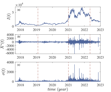
Figure 1: (a) Bitcoin market index $I(t)$ from 03/09/2017 to 31/12/2022. (b) Simple price return $X^{*}(t)$ obtained from $\hat{I}(t)$ following Eq. 4. (c) The standard deviation $\sigma(t)$ of simple price return calculated by using a 1-hour moving window, where $\sigma(t)=\sqrt{\frac{1}{N-1}\sum_{t=1}^{N}(X^{*}(t)-\mu)^{2}}$, $X^{*}_{i}$ indicates a specific segment of the price return, and $\mu$ is the mean value of that segment.

V.1 Anomalous diffusion and fat-tailed distribution

Our analysis commences with an examination of the PDF of simple price return $X(t_{0},t)$ as shown in Eq. 1. For both Period 1 and Period 2, we calculate the PDFs across various time intervals $t=t-t_{0}$, i.e. we plot the relative diffusion time instead of the absolute time, ranging from the smallest diffusion interval $t=1$ to a year’s diffusion period $t=326\,days$. The kernel density estimator, known for its capacity to provide a smooth and accurate estimation of PDFs Wȩglarczyk (2018), is employed with a kernel bandwidth set to 0.001. This ensures that the bandwidth is sufficiently small to capture the detailed structures of the PDFs. To compute the PDFs, we calculate the price return using Eq. 1 for each time interval $t$ and then use the price return to calculate $P(X,t)$.

In Figure 2 (a), we present the peak of the PDF $P_{max}$ for Periods 1 and 2 respectively in relation to time $t$. Notably, both time periods exhibit a power-law relation between the peak of the PDF and time, expressed as $P_{max}\sim t^{-H}$. Linear curve fitting is applied to the data of Periods 1 and 2 respectively to measure the power-law slope ($H=1/\alpha$). We note a transition in the $H$ values for both datasets is observed, signifying a shift in the diffusion mode. For Period 1, the Hurst exponent $H$ is $0.415\pm 0.006$ at small time intervals and $0.610\pm 0.007$ at large time intervals, corresponding to the values of $\alpha=2.41\pm 0.03$ and $\alpha=1.64\pm 0.02$, respectively. For Period 2, the slope is $H=0.478\pm 0.004$ at small time intervals and $H=0.646\pm 0.004$ at large time intervals, corresponding to the respective values of $\alpha=2.09\pm 0.01$ and $\alpha=1.54\pm 0.01$. The anomalous diffusion exponent $\alpha$ is used to distinguish normal (Brownian, $\alpha=2,H=0.5$) from anomalous diffusion ($\alpha\neq 2,H\neq 0.5$). The regimes of super- and subdiffusion correspond to $\alpha>2,H<0.5$ and $0<\alpha<2,H>0.5$, respectively Sposini et al. (2022b). These results suggest that both periods of the Bitcoin time series undergo a transition from a weak subdiffusion regime to a weak superdiffusion regime over an extended period.

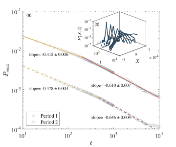
Figure 2: (a) Time evolution of the peak of the PDF for Period 1 and 2 in the log-log scale shown in Black markers. Two well-defined slopes can be observed for each period. The colored lines show the fitted slope of the power-law relation. Both periods experience a transition from a weak subdiffusion regimen to a weak superdiffusion regime over time. (b) Time evolution of the PDF for Period 2 from 10 mins to 1000 mins. The PDFs present distinctive peaks and heavy tails at small time intervals and become flat as the time interval increases.

Figure 2 (b) illustrates the time evolution of the PDF from 10 minutes to 1000 minutes (approximately 16.5 hours) of trading time. The PDF at the minimal time interval $t=1$ exhibits a heavy-tailed non-Gaussian distribution, gradually flattening and broadening as time progresses. To further explore the fat-tailed distribution of the PDF, it is essential to determine the tail slope of the PDF at the minimum time interval, $P(X^{*},t=1)$. This slope, denoted as $\alpha$, is crucial for characterizing the type of distribution. The tail exponent for Lévy distribution is calculated as $P(x,t)\sim x^{-(1+\alpha)}$, where $0<\alpha<2$ Lèvy (1937); Mantegna and Stanley (1994). The exponent for the $q$-Gaussian distribution is $P(x,t)\sim x^{\alpha}$, where $\alpha=\frac{2}{1-q}$, and $1<q<3$ Alonso-Marroquin et al. (2019). In Figure 3, we present the calculated tail slopes of the PDF for each period. The slopes of the tails for Period 1 and Period 2 are $\alpha=3.95\pm 0.18$ and $\alpha=4.04\pm 0.12$ respectively. By comparing these values with the corresponding exponents of Lévy and $q$-Gaussian distribution, we find that the slopes fall outside the Lévy regime and instead fit well into the $q$-Gaussian regime. The values of $q$ calculated based on the derived tail slopes using the aforementioned relation are $q=1.51\pm 0.02$ and $q=1.50\pm 0.02$ for Period 1 and 2, respectively.

Upon examining the fat-tailed distribution, we discerned that the PDF at the minimum time interval ($t=1$) can be characterized by a $q$-Gaussian distribution. To substantiate this observation, we conducted a calibration to the $q$-Gaussian distribution for the PDFs corresponding to both Period 1 and Period 2. The outcomes of this calibration process are depicted in Figure 4. This calibration procedure was conducted in a semi-logarithmic scale by applying the relationship described in Eq. 10. This method involved taking the natural logarithm of the PDF and fitting it to the simple price return using a linear scale. Figure 4 (a) plots the right branch of the PDF using a log-log scale and Figure 4 (b) illustrates both branches of the PDF in semi-logarithmic scale. In these figures, the grey dotted curves represent the PDF of the simple price return, while the Black curves represent the fitted $q$-Gaussian distribution. Notably, the fitted distribution captures both the central and tail portions of the PDFs. The $q$ values derived from the semi-logarithmic fitting were determined as $q=1.53$ for Period 1 and $q=1.57$ for Period 2. Importantly, these values align with the $q$ values fitted from the power-law tail slope, affirming the consistency of the results that the diffusion is $q$-Gaussian.

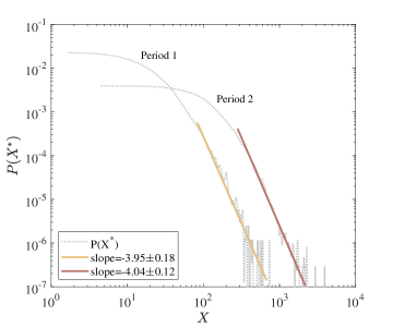
Figure 3: Tail slope of PDF at the minimum time interval $t_{0}$ for Period 1 and 2 respectively in log-log scale. The dotted grey lines are the PDFs of price return, and the colored lines show the fitted slope of the tail for each time period. The fitted slopes show that the tail slope is outside the Lévy regime, and fits to a $q$-Gaussian distribution.

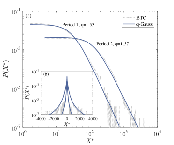
Figure 4: $q$-Gaussian fitting conducted in semi-log scale for PDFs of simple price return at $t_{0}$ for both Period 1 and 2. The grey dotted curves are the PDFs and the Black curves are the fitted $q$-Gaussian distribution. (a) The right branch of the PDFs for Period 1 and 2 are plotted in log-log scale respectively. (b) The full PDF and the fitted distribution are plotted in a semi-log scale.

V.2 Volatility clustering

We use the autocorrelation function (ACF) to quantify volatility clustering in the time series. The ACF is calculated on the incremental price return $X^{*}(t)$ using two methods: sample autocorrelation and chopping autocorrelation. The detailed definitions for each method are presented below.

The time lag of the autocorrelation is denoted as $s$, representing real-time intervals in minutes for this study. For each $s$, the sample autocorrelation is defined as

$$C(s)=\frac{\sum_{t=1}^{n-s}(X^{*}_{t+s}-\bar{X^{*}})(X^{*}_{t}-\bar{X^{*}})}{\sum_{t=1}^{n}(X^{*}_{t}-\bar{X^{*}})^{2}},$$ (26)

where $X^{*}$ is the simple price return, $X^{*}_{t+s}$ is the price return shifted by $s$ minutes, and $\bar{X^{*}}$ is the mean value of the price return, calculated as

$$\bar{X^{*}}=\frac{1}{n}\sum_{t=1}^{n}X^{*}_{t}.$$

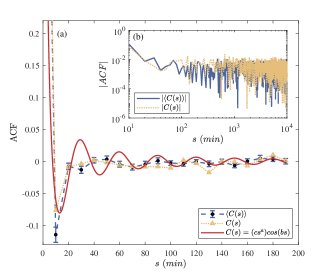
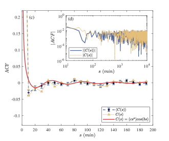
Figure 5: Sample and chopping autocorrelation with fitting for Periods 1 and 2. For both periods, anti-correlation is observed for short times, and weak long-term autocorrelation is presented. (a) For Period 1, chopping ACF is plotted in blue, and sample ACF is plotted in yellow. Anti-correlation is observed in short times with periodicity. The solid red line shows the fitting of the ACFs. Fitting parameters are $a=-1.17,b=0.21,c=1.76$. (b) Absolute sample and chopping ACF of Period 1 plotted in log-log scale, representing a power-law relation. (c) For Period 2, chopping ACF is plotted in blue, and sample ACF is plotted in yellow. Anti-correlation is also observed in short times with periodicity. The solid red line shows the fitting of the ACFs. Fitting parameters are $a=-1.07,b=0.13,c=0.40$. (d) Absolute sample and chopping ACF of Period 2 plotted in log-log scale, with a power-law relation at initial times.

We also computed the chopping autocorrelation of the price return for both periods, following the concept of calculating the ensemble autocorrelation. In the context of stochastic processes, the ensemble represents the statistical population of the process, where each member of the ensemble is one possible realization of the process McCauley (2008); Lahiri (2016). For finance data where only a singular historical time series exists, constructing this ensemble involves decomposing the time series into an ensemble of sub-intervals of the data. Here, each trading day effectively constitutes one realization of the dataset, given the recurring nature of market statistics on a daily basis Bassler et al. (2007). To build the ensemble in our study, we partitioned the data into discrete segments, where each segment serves as an independent realization of the time series. The total length of the time series for the price return is denoted as $N$, while the length of each segment is represented as $S$, and thus the number of segments is $N_{s}=N/S$. The chopping autocorrelation is formulated as

$$\langle C_{s}\rangle=\frac{C_{s}^{i}}{N_{s}},$$ (27)

where $C_{s}^{i}$ corresponds to the $i$^th segment within the ensemble. In the typical practice of establishing the ensemble, each segment is often delineated based on individual trading days. However, due to the continuous nature of the Bitcoin market, we chose to employ calendar weeks as the partitioning markers for our dataset. Given that our data is recorded at 10-minute intervals, resulting in 6 data points recorded per hour and $1,008$ data points accumulated each week. We rounded this to 1,000 data points for the length of each segment. Subsequently, we computed the autocorrelation for each segment and averaged it over the ensemble. The error associated with the ensemble autocorrelation was calculated as the standard error within the ensemble.

The results of the ACF calculated with both methods are presented in Figure 5 for Periods 1 and 2, respectively. The sample autocorrelation is plotted in yellow, while the chopping autocorrelation is in blue. The absolute sample autocorrelation functions are illustrated in Figure 5 (b) and (d) using a log-log scale, corresponding to Periods 1 and 2 respectively. In both time periods, a noticeable power-law relationship emerges, particularly evident at short time intervals (below 100 minutes). Over the longer term, the absolute autocorrelation exhibits a modest yet non-negligible value, persisting notably beyond the 200-minute mark ($C(s)=0.002$ for larger $s$). To quantitatively assess this power-law behavior, we conducted linear curve fitting, obtaining slope values of $-1.17$ for Period 1 and $-1.07$ for Period 2. This slope of absolute autocorrelation is related to the Hurst exponent ($H$), a relationship established as $C(s)\sim s^{-2-2H}$ Kantelhardt et al. (2002). By calculating the Hurst exponent from the power-law slope of the absolute autocorrelation, we obtain the respective values of the Hurst exponent for Periods 1 and 2 as $H=0.415$ and $H=0.486$. Notably, these values align with the findings detailed in Section V.1. To further examine the behavior of the short-time autocorrelation, we plot the ACF for the first 200 minutes in Figure 5 (a) and (c). Both sample and chopping autocorrelation show negative values at short time lags, indicating an anti-correlated relationship in short time frames. Additionally, ACFs manifest periodic oscillations around 0 from 30 minutes to 200 minutes (approximately 2.5 hours), yet the period is different for each time period. While both the sample autocorrelation and chopping autocorrelation exhibit similar characteristics in general, they differ in terms of magnitude. Although there are disparities between the two, these differences are not substantial enough to definitively conclude whether they indicate non-ergodic behavior in the time series or are simply a result of statistical noise.

To systematically capture both the power-law and periodic components in the ACF, we employed a two-step calibration approach for the chopping autocorrelation. First, we applied linear regression to determine the slope characterizing the power-law relationship in the absolute chopping autocorrelation. Secondly, we incorporated a cosine function to account for the periodic behavior. The following relation was used to model the ensemble autocorrelation:

$$<\hat{C}(s)>=(cs^{a})\text{cos}(bs)$$ (28)

where $b$ and $c$ represent the fitting parameters, and $a$ corresponds to the slope derived from the power-law fitting of the absolute chopping autocorrelation. The least-squared curve fitting was performed to find the parameters, and the resulting fitted curves are plotted in red in Figure 5 (a) and (c). Fitting results show that for Period 1, $a=-1.17,b=0.21$, and $c=1.76$, whereas for Period 2, results are $a=-1.07,b=0.13$, and $c=0.40$. Parameter $b$ is related to the periodicity of the observed fluctuation. The fitted results indicate that for Period 1, the period is approximately 60 minutes, whereas in Period 2, the period is 50 minutes.

V.3 Self-similarity of detrended PDF of price return

While the previous section focused on the stylized facts within the trended time series, it is important to note that the underlying trend inherent in financial data can potentially influence these characteristics. To address this, we now redirect our attention to exploring the stylized facts in the detrended time series. In previous sections, we found that for the Bitcoin market index, the market characteristics for Periods 1 and 2 are similar. From here, we focus the analysis on Period 2 only.

Self-similarity in the evolution of the PDF of price return is another important stylized fact in the stock market. We first tested the self-similarity of the trended time series, yet it does not present clear self-similar behavior. Thus, the detrending process is required following the relation described in Eq 3.

V.3.1 Detrending time series

The detrending process was conducted using the Moving Average (MA) method. In MA, a time window is shifted from the start to the end of the time series, and the arithmetic average is used for each time window to record the trend. The two parameters that are vital to the MA are the size of the time window $t_{w}$ and the step in which each time window is shifted forward. In this analysis, we used a continuous sliding window with overlaps, thus the step is 1. These time windows are extended from a segment of $[t,\,\,\,t+t_{w}]$ to the consecutive window of $[t+1,\,\,\,t+t_{w}+1]$. To achieve an effective detrending result, it is necessary to select an optimal time window $t_{w}$ for detrending. In this study, the criteria for choosing the optimal time window are set so that the PDFs of the detrended price return $P(x^{*},t)$ show the best convergence to a Gaussian distribution at large time intervals $t$ and the goodness of fit ($R^{2}$) indicates a valid fitting ($R^{2}\geq 0.95$) for all PDFs.

We tested the time window for detrending from 1 hour to 26 weeks in order to find the best time window that meets the criteria. The optimal time window $t_{w}$ of 1 week is chosen for detrending, and for each time window, the arithmetic average of the index $I(t)$ from $[t,\,\,\,t+t_{w}]$ is used as the trend at time $t$. Considering at the beginning and the end of the time series where $t<\frac{t_{w}}{2}$ and $t>N-\frac{t_{w}}{2}$ ($N$ is the total length of the time series), the size of the time window is truncated, we define the sliding window with three pieces:

$\bullet$ For $t<\frac{t_{w}}{2}$

$$\hat{I}(t)=\frac{2}{t_{w}+2t}{\sum_{k=-t+1}^{\lceil(t_{w}-1)/{2}\rceil}I(t+k)},$$ (29)

$\bullet$ For $\frac{t_{w}}{2}<t<N-\frac{t_{w}}{2}$

$$\hat{I}(t)=\frac{1}{t_{w}}{\sum_{k=-\lfloor(t_{w}-1)/{2}\rfloor}^{\lceil(t_{w}-1)/{2}\rceil}I(t+k)},$$ (30)

$\bullet$ For $t>N-\frac{t_{w}}{2}$

$$\hat{I}(t)=\frac{2}{2N-2t+t_{w}}{\sum_{k=-\lfloor(t_{w}-1)/{2}\rfloor}^{\lceil N-t\rceil}I(t+k)},$$ (31)

with the time step of $t=1,2,3....N$ for the index fluctuations.

The results of detrending are shown in Figure 6. Subfigure 6-a presents the trended market index $I(t)$ as the blue curve and the trend $\bar{I}(t)$ in red after applying MA analysis using the optimal time window of 1 week. Subfigure 6-b shows the detrended price as a result of subtracting the trend, following Eq 2. Subfigure 6-c shows the detrended price return by taking the difference of the adjacent terms in the detrended price, using Eq. 4

$$x^{*}(t)=\hat{I}(t+1)-\hat{I}(t).$$

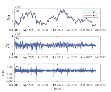
Figure 6: Results from detrending analysis for Period 2. (a) Trended price index $I(t)$ is shown as the blue curve, and the trend $\bar{I}(t)$ obtained from the MA is shown as the red curve. (b) The detrended price index $\hat{I}(t)$ was obtained by subtracting the trend from the price index. (c) Detrended price return $x^{*}(t)$ calculated from the detrended price index.

V.3.2 Self-similarity in PDF of detrended price return

We then test the self-similarity on the detrended price return. Recall the expression of the PDF to be:

$$P(x,t)=\dfrac{1}{(Dt)^{H}}\left[g_{q}\left(\dfrac{x}{(Dt)^{H}}\right)\right]$$

where $(Dt)^{H}$ is the scaling factor, and $H=1/\alpha$ is the Hurst exponent, and is related to the parameter characterizing the anomalous diffusion. Taking the result of $H=0.478$ in Section V.1 for time series Period 2, we conducted the $q$-Gaussian fitting to the detrended PDFs at each time $t$ of price return in a semi-log scale, with two fitting parameters $q$ and $\beta=(Dt)^{1/\alpha}$ to find the scaling factor. The PDFs are rescaled using these factors, and the resultant PDFs were collapsed onto each other as shown in the grey curves in Figure 7. The collapsed PDF shows a good agreement with the $q$-Gaussian distribution with $q=1.51$, shown as the blue curve.

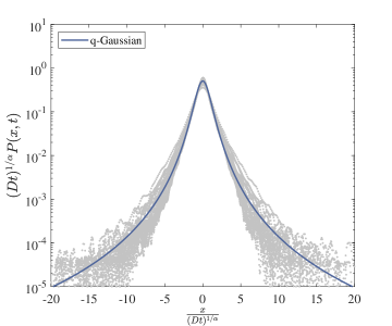
Figure 7: (Grey curves) Collapse of the PDF of detrended price return for Bitcoin Period 2. The collapsed PDFs are fitted with a $q$-Gaussian distribution (blue curve) with $q=1.51$.

V.4 Scaling Analysis on the Fractality of Price Return

In the preceding sections, we have demonstrated the presence of self-similarity in Bitcoin price returns, suggesting a fractal nature of the time series. In this section, we aim to establish whether the time series is monofractal or multifractal by performing a scaling analysis. In the latter scenario, self-similarity is preserved, but the Hurst exponent is not unique. Instead, it exhibits a range of values forming a Hurst exponent profile.

Various methods can demonstrate the fractality of a time series, with commonly used approaches including rescaled range (R/S) analysis and detrended fluctuation analysis (DFA). Currently, DFA is becoming a more favored method because of its effectiveness in handling nonstationary time series. In our study, we applied DFA to Bitcoin Period 2 to determine fractality and calculate the Hurst exponent. DFA was performed on the trended time series. The first step of DFA involves removing the trend of the original time series by assuming the trend is the linear fitting of each non-overlapping segment.

$\bullet$ Step 1

For the trended price return with length $N$, the process of the DFA starts with defining the ‘profile’ of the time series by calculating the mean-centered cumulative sum of the simple price return ($X$):

$$I^{*}(t)=\sum_{k=1}^{i}\left[X_{k}-\langle X\rangle\right],i=1,...,N.$$ (32)

where $\langle X\rangle$ is the mean value of the time series.

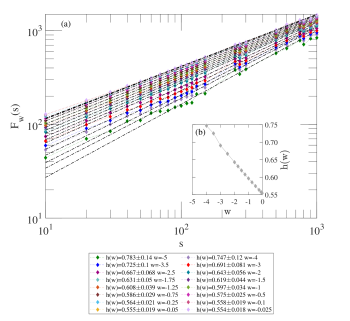
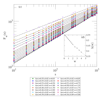
Figure 8: Calculation of the statistical function $F_{w}$ on Bitcoin price return for Period 2 using Eq. (34). The function of $F_{w}$ vs $s$ display power laws $F_{w}(s)\sim s^{h(w)}$, where $h(w)$ depend on $w$. This feature demonstrates that the time series is multifractal. (a) Calculated $F_{w}(s)$ function with a negative range of $w$, each $w$ value presents a power-law relationship. (b) Profile of $h(w)$ for negative $w$ values. (c) Calculated $F_{w}(s)$ function with a positive range of $w$, each $w$ value presents a power-law relationship. (d) Profile of $h(w)$ for positive $w$ values.

The second part of DFA aims to calculate the scaling function $F_{w}(s)$ as a function of the time segment $s$, and $w$ is the order of the mathematical moment. This is achieved by applying the following steps:

$\bullet$ Step 2

Divide the profile $I^{*}(t)$ into non-overlapping segments with the same length $s$. The number of segments $N_{s}$ is calculated as $N_{s}=\lfloor N/s\rfloor$.

$\bullet$ Step 3

Calculate the local trend for each segment by a linear least-square fitting of the time series. Then the variance of each segment $v$ from $1,2,3....N_{s}$ is calculated using the equation:

$$F^{2}(v,s)=\frac{1}{s}{\sum_{i=1}^{s}(I^{*}[(v-1)s+i]-\overline{I^{*}}(v,s))^{2}},$$ (33)

where $\overline{I^{*}}(v,s)$ is the mean of each segment of $I^{*}(t)$.

$\bullet$ Step 4

The statistical moments are calculated utilizing different values of order $w$:

$$F_{\mathrm{w}}(s)=\left\{\frac{1}{N_{s}}{\sum_{i=1}^{N{s}}[F^{2}(v,s)]^{\mathrm{w}/2}}\right\}^{1/\mathrm{w}}$$ (34)

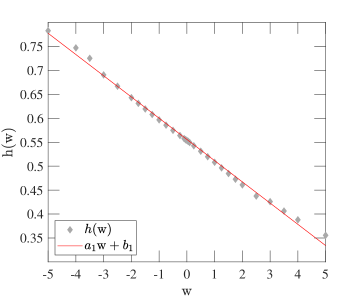
Figure 9: Evaluation of the scale exponents $h_{w}$ of detrended Bitcoin price return for Period 2. This profile of scale exponent can be described using a linear relationship, with $a1=-0.044\pm 0.006$, and $b1=0.556\pm 0.002$. The Hurst exponent is equivalent to the $h(2)$ value, from which $H=0.461$.

For detrended time series that present long-range correlations, the following power law is obtained: $F_{w}(s)\sim s^{h(w)}$. If the time series is monofractal, $h(w)$ is independent of $w$ value thus a constant is obtained where $H=h(w)$ is the Hurst exponent. For multifractal time series, $h(w)$ is dependent on $w$ and can be a linear or quadratic function.

Results of the DFA are shown in Figure 8 for positive and negative range of $w$ respectively. A linear fitting is conducted for each order of $w$ to obtain the power law and plotted as the dashed black lines. It is clear that the slope of $h(w)$ varies for different $w$, indicating that the time series is multifractal. Figure 9 plots the resultant spectrum for the Hurst exponent, where $h(2)$ is the Hurst exponent representing the time series Kantelhardt et al. (2002). For Period 2, $H=0.461$, which agrees with the results obtained in the previous sections.

VI Discussion

Table 1: Summary of stylized facts

Stylized Facts	Period 1	Period 2	S&P500
Fat-tailed Distribution $P(x,t)\sim x^{\frac{2}{1-q}}$ for large $x$	$q=1.51$	$q=1.50$	$q=1.50$
Anomalous Diffusion $P(x=0,t)\sim t^{-H},H=1/\alpha$	$H=0.415$ $\alpha=2.41$	$H=0.478$ $\alpha=2.09$	$H=0.79$ $\alpha=1.26$
$q$-Gaussian Diffusion $P(x,t)=\dfrac{1}{(Dt)^{H}}\left[g_{q}\left(\dfrac{x}{(Dt)^{H}}\right)\right]$	$q=1.53$	$q=1.57$	$q=1.71$ $q=2.73$
Volatility Clustering $C(s)\sim(cs)^{2H-2}\text{cos}(bs)$	$H=0.415$	$H=0.465$	$C(s)\sim e^{-\rho s}$ $\rho=1.07$
Scaling Analysis $F_{w}(s)\sim s^{h(w)},H=h(2)$	/	$H=0.461$	$H=0.48$

We investigated the stylized facts of the Bitcoin time series from 2019 to 2022. The Bitcoin price index was divided into two periods based on changes in volatility. Table 1 summarizes the stylized facts observed in the Bitcoin price index. Here we compare the results of the Bitcoin price index to the well-studied conventional market S&P500 for the period from January 1996 to May 2018.

The prevalence of a heavy-tailed distribution is a characteristic feature in traditional financial markets, such as the S&P500. In line with this, we found fat-tailed distribution for both time periods of Bitcoin price return. This finding aligns with previous studies on cryptocurrencies, where the majority of types of cryptocurrencies exhibit heavy-tailed non-Gaussian distributions Zhang et al. (2018). Our study extends previous findings by illustrating that the PDF of Bitcoin’s price return is best captured by a $q$-Gaussian distribution, making these results directly comparable with our previous results for the S&P500. Specifically, we find $q=1.51\pm 0.02$ for Period 1 and $q=1.50\pm 0.02$ for Period 2.

In comparison to the S&P500 index, the anomalous diffusion of Bitcoin presents distinctive characteristics. While Bitcoin and the S&P500 have undergone a shift in diffusion behavior, their respective diffusion patterns differ. For the S&P500 price return, research has shown that it displays a strong superdiffusion regime with $\alpha=1.26\pm 0.04\,(H=0.79)$ for short time intervals, and in the long term, it exhibits a weak superdiffusion regime with $\alpha=1.79\pm 0.01\,(H=0.56)$ Alonso-Marroquin et al. (2019). In contrast, Bitcoin price returns exhibit a transition in diffusion behavior in both periods, shifting from a subdiffusion regime to a weak superdiffusion regime. In Period 1, $\alpha=2.41\pm 0.02\,(H=0.415)$ for short time intervals, and $\alpha=1.64\pm 0.02\,(H=0.610)$ for extended time intervals. In Period 2, short time intervals reveal $\alpha=2.09\pm 0.01,(H=0.478)$, while extended time intervals exhibit $\alpha=1.54\pm 0.01,(H=0.646)$. Notably, the diffusion parameters indicate that Period 1 of Bitcoin demonstrates a more pronounced subdiffusion than Period 2 for short time intervals. The anomalous diffusion of Bitcoin can be described by a $q$-Gaussian diffusion process, similar to the findings of S&P500. However, the values of the $q$ parameter are different between the two markets. For S&P500, the $q$-Gaussian exponents are $q=1.71\pm 0.01$ and $q=2.73\pm 0.005$ for the two diffusion regimes, respectively Alonso-Marroquin et al. (2019). Conversely, for Bitcoin, the $q$-Gaussian exponents are notably lower, at approximately $q=1.55\pm 0.02$ for both Periods 1 and 2.

The autocorrelation functions are calculated based on the price returns of Bitcoin. Regarding the ACF for absolute returns, it demonstrates a power-law decay, with the calculated Hurst exponents shifting from less than 0.5 in Period 1 ($H=0.415$) to slightly closer to 0.5 in Period 2 ($H=0.486$). In terms of the ACF of price returns, both time periods exhibit short-term negative autocorrelation. This negative autocorrelation rapidly diminishes and fluctuates around zero, with different amplitudes and periods for each time period. The autocorrelation in small intraday time scales (less than $20$ minutes) can be attributed to the microstructure effects of the market Cont (2001). This negative autocorrelation aligns with the findings on feedback traders in Bitcoin Karaa et al. (2021), confirming that the high volatility and positive trading strategy can yield significant anti-autocorrelations in market dynamics. The ACF pattern observed in Bitcoin price return differs from the observations in S&P500; in the case of S&P500, the ACF presents an exponential pattern at short times, then transitions to a power-law relationship Arias-Calluari et al. (2022).

From the scaling analysis, we found that both time periods of the Bitcoin price index are multi-fractal, which aligns with other studies on the fractality of the Bitcoin market Takaishi (2018); Shrestha (2021). This multi-fractality characteristic is similar to the observations in the traditional financial markets and other complex systems Lee et al. (2017); Mali and Mukhopadhyay (2014); Wang et al. (2013); Gu et al. (2010); Chen et al. (2016). The multi-fractal nature of Bitcoin can be attributed to the presence of volatility clusters varying across different time scales and fat-tail distributions, as these aspects make essential contributions to multi-fractality in a given time series Lahmiri and Bekiros (2018).

References

- Corbet et al. (2019) S. Corbet, B. Lucey, A. Urquhart, and L. Yarovaya, International Review of Financial Analysis 62, 182 (2019).
- Crosby et al. (2016) M. Crosby, P. Pattanayak, S. Verma, and V. Kalyanaraman, Applied Innovation 2, 71 (2016).
- Noam (2021) E. Noam, The Macro-Economics of Crypto-Currencies: The Role of Private Moneys in Monetary Policy, 23rd ITS Biennial Conference, Online Conference / Gothenburg 2021. Digital societies and industrial transformations: Policies, markets, and technologies in a post-Covid world 238043 (International Telecommunications Society (ITS), 2021).
- Nakamoto (2008) S. Nakamoto, “A peer-to-peer electronic cash system,” (2008).
- Coi (2023) “Global cryptocurrency charts,” https://coinmarketcap.com/charts/ (2023), accessed: 2023-08-03.
- Underwood (2016) S. Underwood, Communications of the ACM 59, 15 (2016).
- Zaghloul et al. (2020) E. Zaghloul, T. Li, M. W. Mutka, and J. Ren, IEEE Internet of Things Journal 7, 10288 (2020).
- Hong (2017) K. Hong, Information Technology and Management 18, 265 (2017).
- Baur et al. (2015) D. G. Baur, A. D. Lee, and K. Hong (2015).
- Popper (2016) N. Popper, Digital Gold: Bitcoin and the Inside Story of the Misfits and Millionaires Trying to Reinvent Money (HarperCollins, 2016).
- Henriques and Sadorsky (2018) I. Henriques and P. Sadorsky, Journal of Risk and Financial Management 11, 48 (2018).
- Genç (2023) E. Genç, “How are institutions and companies investing in crypto?” (2023).
- Auer et al. (2023) R. Auer, B. Haslhofer, S. Kitzler, P. Saggese, and F. Victor, The Technology of Decentralized Finance (DeFi) (Bank for International Settlements, Monetary and Economic Department, 2023).
- Urquhart (2016) A. Urquhart, Economics Letters 148, 80 (2016).
- Kurihara and Fukushima (2017) Y. Kurihara and A. Fukushima, Journal of Applied Finance and Banking 7, 57 (2017).
- Jiang et al. (2018) Y. Jiang, H. Nie, and W. Ruan, Finance Research Letters 25, 280 (2018).
- Caporale et al. (2018) G. M. Caporale, L. A. Gil-Alana, and A. Plastun, SSRN Electronic Journal (2018), 10.2139/ssrn.3126040.
- Noda (2021) A. Noda, Applied Economics Letters 28, 433 (2021).
- Bariviera et al. (2017) A. F. Bariviera, M. J. Basgall, W. Hasperué, and M. Naiouf, Physica A: Statistical Mechanics and its Applications 484, 82 (2017).
- Mnif et al. (2020) E. Mnif, A. Jarboui, and K. Mouakhar, Finance Research Letters 36, 101647 (2020).
- Mnif and Jarboui (2021) E. Mnif and A. Jarboui, Review of Behavioral Finance 13, 69 (2021).
- Fernandes et al. (2022) L. H. S. Fernandes, E. Bouri, J. W. L. Silva, L. Bejan, and F. H. A. de Araujo, Physica A: Statistical Mechanics and its Applications 607, 128218 (2022).
- Montasser et al. (2022) G. E. Montasser, L. Charfeddine, and A. Benhamed, Finance Research Letters 46, 102362 (2022).
- Kakinaka and Umeno (2022) S. Kakinaka and K. Umeno, Finance Research Letters 46, 102319 (2022).
- Brito et al. (2014) J. Brito, H. Shadab, and A. Castillo, Columbia Science and Technology Law Review 16, 144 (2014).
- Böhme et al. (2015) R. Böhme, N. Christin, B. Edelman, and T. Moore, Journal of Economic Perspectives 29, 213 (2015).
- Hendrickson and Luther (2017) J. R. Hendrickson and W. J. Luther, Journal of Economic Behavior & Organization 141, 188 (2017).
- Marian (2013) O. Marian, Michigan Law Review First Impressions 112, 38 (2013).
- Gross et al. (2017) A. Gross, J. Hemker, J. Hoelscher, and B. Reed, Journal of Accounting Education 39, 48 (2017).
- Conrad et al. (2018) C. Conrad, A. Custovic, and E. Ghysels, Journal of Risk and Financial Management 11, 23 (2018).
- Ciaian et al. (2018) P. Ciaian, M. Rajcaniova, and d. Kancs, Journal of International Financial Markets, Institutions and Money 52, 173 (2018).
- Klein et al. (2018) T. Klein, H. Pham Thu, and T. Walther, International Review of Financial Analysis 59, 105 (2018).
- Eross et al. (2019) A. Eross, F. McGroarty, A. Urquhart, and S. Wolfe, Research in International Business and Finance 49, 71 (2019).
- Ariya et al. (2020) K. Ariya, N. Naktnasukanjn, T. Rattanadamrongaksorn, P. Udomwong, S. Sokantika, and N. Chakpitak, Proceedings - 2020 15th International Joint Symposium on Artificial Intelligence and Natural Language Processing, iSAI-NLP 2020 (2020), 10.1109/iSAI-NLP51646.2020.9376813.
- Arias-Calluari et al. (2021) K. Arias-Calluari, F. Alonso-Marroquin, M. N. Najafi, and M. Harré, Physica A: Statistical Mechanics and its Applications 568, 125587 (2021).
- Hu et al. (2019) A. S. Hu, C. A. Parlour, and U. Rajan, Financial Management 48, 1049 (2019).
- De Sousa Filho et al. (2021) F. N. M. De Sousa Filho, J. N. Silva, M. A. Bertella, and E. Brigatti, Brazilian Journal of Physics 51, 576 (2021).
- Cremaschini et al. (2023) A. Cremaschini, A. Punzo, E. Martellucci, and A. Maruotti, Applied Economics 55, 3675 (2023).
- Ghosh et al. (2023) B. Ghosh, E. Bouri, J. B. Wee, and N. Zulfiqar, Research in International Business and Finance 65, 101945 (2023).
- Wen et al. (2022) Z. Wen, E. Bouri, Y. Xu, and Y. Zhao, The North American Journal of Economics and Finance 62, 101733 (2022).
- Zhang et al. (2018) W. Zhang, P. Wang, X. Li, and D. Shen, Applied Economics 50, 5950 (2018).
- Cont (2001) R. Cont, Quantitative Finance 1, 223 (2001), doi: 10.1080/713665670.
- Chakraborti et al. (2011) A. Chakraborti, I. M. Toke, M. Patriarca, and F. Abergel, Quantitative Finance 11, 991 (2011).
- Kaldor (1961) N. Kaldor, “Capital accumulation and economic growth,” (Palgrave Macmillan UK, 1961) pp. 177–222.
- Bollerslev et al. (1994) T. Bollerslev, R. F. Engle, and D. B. Nelson, Handbook of econometrics 4, 2959 (1994).
- Nystrup et al. (2015) P. Nystrup, H. Madsen, and E. Lindström, Quantitative Finance 15, 1531 (2015).
- Shakeel and Srivastava (2018) M. Shakeel and B. Srivastava, Global Business Review 22, 550 (2018).
- Rydén et al. (1998) T. Rydén, T. Teräsvirta, and S. Åsbrink, Journal of Applied Econometrics 13, 217 (1998).
- Liesenfeld and Jung (2000) R. Liesenfeld and R. C. Jung, Journal of Applied Econometrics 15, 137 (2000).
- Andersson (2001) J. Andersson, Journal of Business & Economic Statistics 19, 44 (2001).
- Carnero (2004) M. A. Carnero, Journal of Financial Econometrics 2, 319 (2004).
- Bulla and Bulla (2006) J. Bulla and I. Bulla, Computational Statistics & Data Analysis 51, 2192 (2006).
- Malmsten and Teräsvirta (2010) H. Malmsten and T. Teräsvirta, European Journal of pure and applied mathematics 3, 443 (2010).
- Segnon and Bekiros (2020) M. Segnon and S. Bekiros, Annals of Finance 16, 435 (2020).
- Mandelbrot (1963) B. Mandelbrot, The Journal of Business 36 (1963).
- Stoyanov et al. (2011) S. V. Stoyanov, S. T. Rachev, B. Racheva-Yotova, and F. J. Fabozzi, The Journal of Portfolio Management 37, 107 (2011).
- Lèvy (1937) P. Lèvy, Thèorie de lÀddition des Variables Alèatoires (Gauthier–Villars, Paris, 1937).
- Mantegna and Stanley (1994) R. N. Mantegna and H. E. Stanley, Physical Review Letters 73, 2946 (1994).
- Mantegna and Stanley (1999) R. N. Mantegna and H. E. Stanley, Introduction to econophysics: correlations and complexity in finance (Cambridge university press, 1999).
- Borland and Bouchaud (2004) L. Borland and J.-P. Bouchaud, Quantitative Finance 4, 499 (2004), doi: 10.1080/14697680400008684.
- Queirós (2005) S. M. D. Queirós, Quantitative Finance 5, 475 (2005), doi: 10.1080/14697680500244403.
- Malamud (2003) B. Malamud, Physics World 17, 31 (2003).
- Alonso-Marroquin et al. (2019) F. Alonso-Marroquin, K. Arias-Calluari, M. Harré, M. N. Najafi, and H. J. Herrmann, Physical Review E 99, 062313 (2019).
- Gharari et al. (2021) F. Gharari, K. Arias-Calluari, F. Alonso-Marroquin, and M. N. Najafi, Physical Review E 104, 054140 (2021).
- Tang et al. (2023) Y. Tang, F. Gharari, K. Arias-Calluari, F. Alonso-Marroquin, and M. N. Najafi, “Variable order porous media equations: Application on modeling the s&p500 and bitcoin price return,” (2023), arXiv:2309.04206 [cond-mat.stat-mech] .
- Vilela et al. (2013) M. Vilela, N. Halidi, S. Besson, H. Elliott, K. Hahn, J. Tytell, and G. Danuser, in Fluorescence Fluctuation Spectroscopy (FFS), Part B, Methods in Enzymology, Vol. 519, edited by S. Y. Tetin (Academic Press, 2013) pp. 253–276.
- Nounou and Bakshi (2000) M. N. Nounou and B. R. Bakshi, in Wavelets in Chemistry, Data Handling in Science and Technology, Vol. 22, edited by B. Walczak (Elsevier, 2000) pp. 119–150.
- Kasdin (1995) N. J. Kasdin, Proceedings of the IEEE 83, 802 (1995).
- Kumar (2016) R. Kumar, in Valuation, edited by R. Kumar (Academic Press, San Diego, 2016) pp. 47–72.
- De Silva et al. (2017) H. De Silva, G. M. McMurran, and M. N. Miller, in Factor Investing, edited by E. Jurczenko (Elsevier, 2017) pp. 365–387.
- Chen et al. (2016) F. Chen, K. Tian, X. Ding, Y. Miao, and C. Lu, Physica A: Statistical Mechanics and its Applications 462, 1058 (2016).
- Mandelbrot and Mandelbrot (1982) B. B. Mandelbrot and B. B. Mandelbrot, The fractal geometry of nature, Vol. 1 (WH freeman New York, 1982).
- Lee et al. (2017) M. Lee, J. W. Song, J. H. Park, and W. Chang, Chaos, Solitons & Fractals 97, 28 (2017).
- Mali and Mukhopadhyay (2014) P. Mali and A. Mukhopadhyay, Physica A: Statistical Mechanics and its Applications 413, 361 (2014).
- Wang et al. (2013) F. Wang, G. ping Liao, J. hui Li, X. chun Li, and T. jun Zhou, Physica A: Statistical Mechanics and its Applications 392, 5723 (2013).
- Gu et al. (2010) R. Gu, H. Chen, and Y. Wang, Physica A: Statistical Mechanics and its Applications 389, 2805 (2010).
- Önalan (2004) O. Önalan, in 1st International Conference on Computational Finance and its Applications (Bologna, Italy, 2004) pp. 289–295.
- Lahmiri and Bekiros (2018) S. Lahmiri and S. Bekiros, Chaos, Solitons & Fractals 106, 28 (2018).
- Bachelier (1900) L. Bachelier, Annales scientifiques de l’École Normale Supérieure 17, 21 (1900).
- Black and Scholes (1973) F. Black and M. Scholes, Journal of Political Economy 81, 637 (1973).
- Weron and Magdziarz (2009) A. Weron and M. Magdziarz, Europhysics Letters 86, 60010 (2009).
- Sposini et al. (2022a) V. Sposini, D. Krapf, E. Marinari, R. Sunyer, F. Ritort, F. Taheri, C. Selhuber-Unkel, R. Benelli, M. Weiss, R. Metzler, and G. Oshanin, Communications Physics 5 (2022a), 10.1038/s42005-022-01079-8.
- Haber and Stornetta (1991) S. Haber and W. S. Stornetta, in Advances in Cryptology-CRYPTO’ 90, edited by A. J. Menezes and S. A. Vanstone (Springer Berlin Heidelberg, 1991) pp. 437–455.
- Vujičić et al. (2018) D. Vujičić, D. Jagodić, and S. Ranđić, in 2018 17th International Symposium INFOTEH-JAHORINA (INFOTEH) (2018) pp. 1–6.
- Kuo Chuen et al. (2018) D. L. Kuo Chuen, L. Guo, and Y. Wang, The Journal of Alternative Investments 20, 16 (2018).
- Tschorsch and Scheuermann (2016) F. Tschorsch and B. Scheuermann, IEEE Communications Surveys & Tutorials 18, 2084 (2016).
- Arias-Calluari et al. (2022) K. Arias-Calluari, M. N. Najafi, M. S. Harré, Y. Tang, and F. Alonso-Marroquin, Physica A: Statistical Mechanics and its Applications 587, 126487 (2022).
- Itô (1951) K. Itô, Nagoya Mathematical Journal 3, 55 (1951).
- Borland (1998) L. Borland, Physical Review E 57, 6634 (1998).
- Wȩglarczyk (2018) S. Wȩglarczyk, ITM Web of Conferences 23, 00037 (2018).
- Sposini et al. (2022b) V. Sposini, D. Krapf, E. Marinari, R. Sunyer, F. Ritort, F. Taheri, C. Selhuber-Unkel, R. Benelli, M. Weiss, R. Metzler, and G. Oshanin, Communications Physics 5, 305 (2022b).
- McCauley (2008) J. L. McCauley, Physica A: Statistical Mechanics and its Applications 387, 5518 (2008).
- Lahiri (2016) A. Lahiri, “Chapter 7 - optical coherence: Statistical optics,” in Basic Optics, edited by A. Lahiri (Elsevier, Amsterdam, 2016) pp. 605–696.
- Bassler et al. (2007) K. E. Bassler, J. L. McCauley, and G. H. Gunaratne, Proceedings of the National Academy of Sciences 104, 17287 (2007).
- Kantelhardt et al. (2002) J. W. Kantelhardt, S. A. Zschiegner, E. Koscielny-Bunde, S. Havlin, A. Bunde, and H. E. Stanley, Physica A: Statistical Mechanics and its Applications 316, 87 (2002).
- Karaa et al. (2021) R. Karaa, S. Slim, J. W. Goodell, A. Goyal, and V. Kallinterakis, The European Journal of Finance , 1 (2021), doi: 10.1080/1351847X.2021.1973054.
- Takaishi (2018) T. Takaishi, Physica A: Statistical Mechanics and its Applications 506, 507 (2018).
- Shrestha (2021) K. Shrestha, International Review of Finance 21, 312 (2021).