Analyzing the Impact of Design Factors on Solar Module Thermomechanical Durability Using Interpretable Machine Learning Techniques

Abstract

Solar modules in utility-scale PV systems are expected to maintain decades of lifetime to effectively rival the cost of conventional energy sources. However, the long-term performance of these modules is often degraded by cyclic thermomechanical loading, emphasizing the need for a proper module design to counteract the detrimental effects of thermal expansion mismatch between module materials. Given the complex composition of solar modules, isolating the impact of individual components on overall durability remains a challenging task. In this work, we analyze a comprehensive data set capturing bill-of-materials and post-thermal-cycling power loss from over 250 distinct module designs. Using the data set, we develop a machine learning model to correlate the design factors with the degradation and apply the Shapley additive explanation to provide interpretative insights into the model’s decision-making. Our analysis reveals that the type of silicon solar cell, whether monocrystalline or polycrystalline, predominantly influences the degradation, and monocrystalline cells present better durability. This finding is further substantiated by statistical testing on our raw data set. We also demonstrate that the thickness of the encapsulant, particularly the front side one, remains another important factor. While thicker encapsulants lead to reduced power loss, further increasing their thickness does not yield additional benefits. The study moreover provides a blueprint for utilizing explainable machine learning techniques in a complex material system and can potentially steer future research on optimizing solar module design.

I Introduction

Utility-scale photovoltaic (PV) systems are expected to achieve an extended operational lifetime to be competitive with conventional energy sources [1]. However, solar modules installed in the field are subject to multiple environmental stresses such as ultraviolet light, temperature variation, mechanical loading induced by snow, wind, hail [2]. These factors introduce multiple pathways of degradation, reducing the durability of the module. One of the sources of long-term degradation is the cyclic thermomechanical deformation of solar modules caused by temperature variation. Over time, thermal cycling can cause the degradation of components inside solar modules, such as interconnections, and lead to a decrease in module power [2, 3]. Therefore, it is essential to identify the potential problems in the current design of solar modules and optimize module robustness to thermal cycling degradation.

Figure 1(a) illustrates an example of a typical glass/backsheet module. Its multi-layered construction comprises a front frame, a glass layer, polymer encapsulant layers commonly made from ethylene vinyl acetate (EVA) or polyolefin elastomer (POE), a solar cell layer composed of silicon solar cells and copper interconnections, and a backside polymer backsheet made from layers of polyvinyl fluoride, polyethylene terephthalate, and polyvinyl fluoride (TPT). The copper ribbons are connected to the cell metallization with solder (SnPb). A defining characteristic of these components is their distinct thermal expansion coefficients (CTE, $\alpha$). This variance in CTEs means they expand or contract at different rates in response to daily and seasonal temperature fluctuations in their operational environment.

Previous research [4] showed that the power loss of different models of PV modules after extended thermal cycling tests up to 600 cycles varied from 0.8% to 14.5%. Such degradation is partially due to the CTE mismatch between the glass ($\alpha_{glass}\approx 8\times 10^{-6}K^{-1}$) and Si cells ($\alpha_{cell}\approx 2.5\times 10^{-6}K^{-1}$). The cells adhere to the glass by encapsulants, so the CTE mismatch causes a non-uniform in-plane displacement of cells and glass [5]. The gap between cells can vary with different temperatures, as shown in Figure 1(b). Such temperature-driven variations over a module’s lifespan can result in cyclic deformation of copper ribbons that connect cells and cause interconnection fatigue [5, 6, 7]. Additionally, fragments in cracked cells can shift due to temperature variation, leading to wear and tear at metal contacts [8]. Another prevalent degradation mode caused by temperature variation is solder disconnection. The CTE mismatch between the copper ($\alpha_{Cu}\approx 16.7\times 10^{-6}K^{-1}$) ribbon and Si cell ($\alpha_{Si}\approx 2.5\times 10^{-6}K^{-1}$) triggers non-uniform deformations in these layers [9]. As depicted in Figure 1(c), at elevated temperatures, Si and Cu experience tensile and compressive stresses, and at low temperatures, the stresses are reversed, which causes a periodic change of shear stress within the solder layer [9]. This cyclic loading in the solder often culminates in solder disconnection [10, 11, 12]. Solder degradation is one of the failure modes that happen in the early stage of module operation, which can be probed by 600 cycles of thermal cycling accelerated aging tests [4].

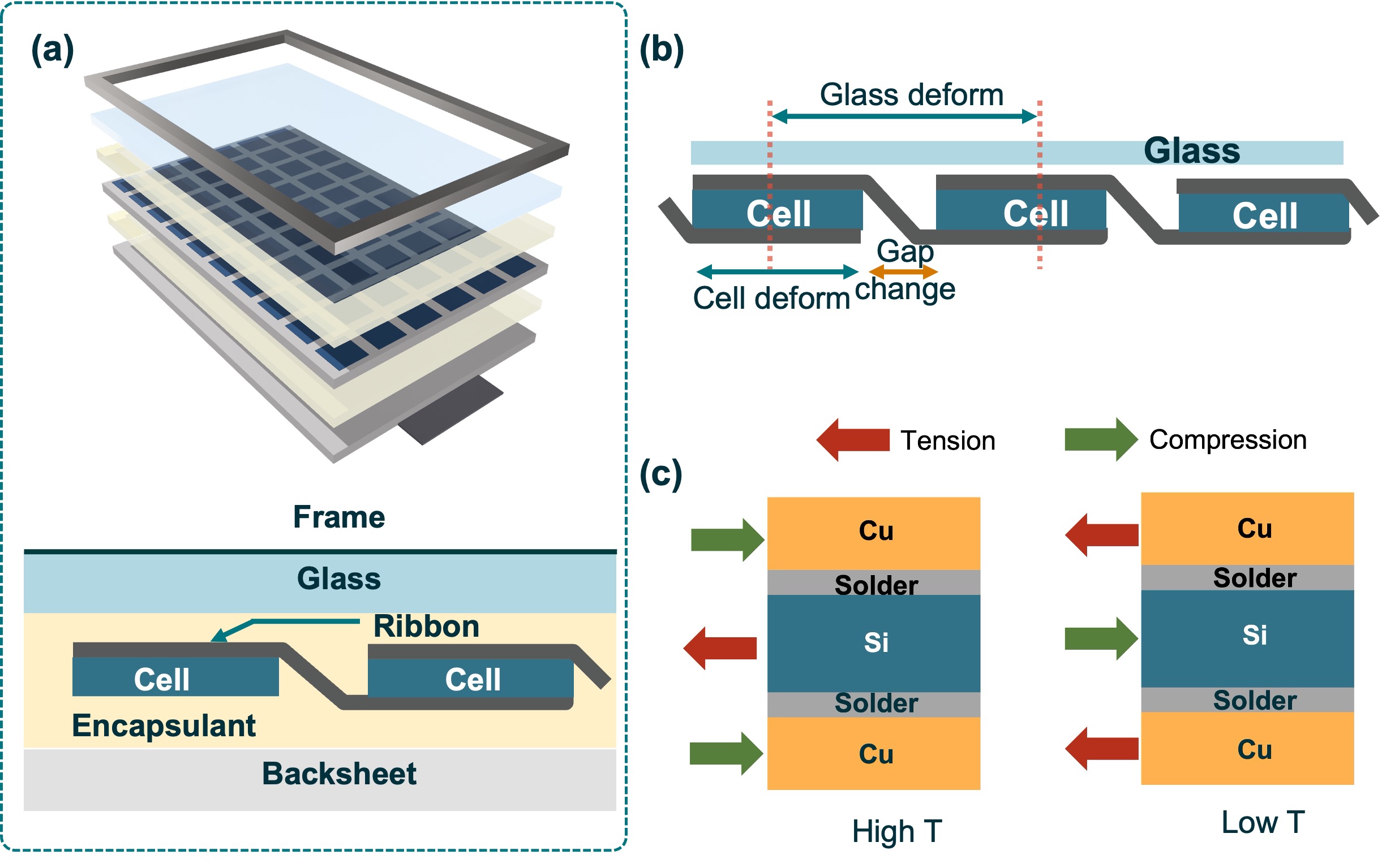
Figure 1: Schematic structure of a glass/backsheet PV module and the mechanism of its thermomechanical degradation. (a) The layered structure of a PV module. (b) Mechanism of the cyclic deformation of ribbons. (c) Mechanism of cyclic thermal stress in solder layer.

As shown above, thermal cycling degradation involves multiple modes, strongly impacted by the specific bill-of-materials (BOM) of solar modules. This encompasses the dimensions and material properties of each module component. Understanding which design factors predominantly affect thermal cycling power loss is of great significance to guide future research on module optimization. Several prior studies have investigated the impact of various design factors. Bosco et al. [13] did a multiple linear regression analysis to identify design factors that may influence the solder degradation by simulating the accumulated damage on the solder joints during thermal cycles. The top sensitive factors are the thickness of the solder layer, Cu ribbon and Si wafer layer. Park et al. [9] also confirmed that reducing Si cell and copper ribbon thickness can increase the solder lifetime in thermal cycling using simulation. Zhu et al. [14] fabricated different mini-modules and did a simulation to investigate the effect of viscoelasticity of encapsulant materials on the solder joint fatigue. They found that modules with encapsulants of higher viscous properties presented more power loss after the thermal cycling test. Beinert et al. [15] found that increasing cell size and changing full cells into half-cut cells could decrease thermal stress on the cell layer using simulation. They further qualitatively concluded that cell thickness, encapsulant CTE and glass/backsheet CTE strongly influence the stress in the cell layer [16]. Hanifi et al. [12] also found that the higher rigidity of encapsulant materials and changing full cells into half-cut cells could mitigate ribbon fatigue during temperature variation. As exemplified by this past research, most sensitivity analysis work in this field relies on simulated data. Computational constraints often force researchers to model simplified structures, like a single cell rather than a comprehensive full-size solar module or ignoring the busbars, which may bypass some real-world effects.

With an outstanding ability to discover the underlying pattern in the data, machine learning (ML) modeling has been increasingly applied to the field of scientific study. While the enhanced predictive accuracy of advanced ML models is commendable, a significant challenge emerges in their interpretability. Several methodologies have been proposed to solve this trade-off between accuracy and interpretability. Noteworthy among these are Partial Dependence Plot (PDP) [17], Local Interpretable Model-agnostic Explanations (LIME) [18], and SHapley Additive exPlanations (SHAP) [19]. In particular, SHAP is able to do both global and local interpretation, and its adoption across diverse scientific disciplines is a testament to its efficacy [20, 21, 22, 23].

In this study, we analyze the impacts of BOM factors on the solar module thermomechanical durability using real-world data. The data comes from PVEL’s product qualification program (PQP) [24]. As part of this comprehensive reliability testing program, PVEL collected full-size commercial solar modules from various manufacturers and manually extracted their design factors from BOM files. The modules were subjected to a suite of accelerated reliability tests, including thermal cycling power loss ($-40^{\circ}\text{C}$ to $+85^{\circ}\text{C}$ for 600 cycles). This program results in a comprehensive data set encompassing both BOM features and corresponding degradation. This data set provides a unique chance to investigate the correlation between BOM features and module durability using real-world data. Next, we develop and compare several ML models to correlate the BOM features with the module’s thermal cycling power loss. The optimal model is the Random Forest (RF) model [25] with a testing root mean square error (RMSE) of 1.179. Subsequently, we use the SHAP method to interpret the developed model and apply statistical testing on the original data set to verify our conclusions. The principal contributions of this study are summarized as follows:

1. Together with PVEL, we publish this processed data set comprising thermal cycling degradation of commercial modules alongside the BOM features for each module. We also publish our fitted models and analysis codes. Some values in this public data set are redacted due to non-disclosure agreement.

2. We provide a comprehensive analysis of the current module design, hoping to provide insights into future research in improving solar module durability.

3. This study establishes a blueprint for interpreting ML models in solar research within a complex system, bridging the gap between data-driven predictions and actionable design insights. The methods present here can be extended to other data-driven projects such as root cause analysis of field current-voltage data of a PV system.

The rest of this article is organized as follows: Section II illustrates the details of thermal cycling setup and computation methodologies, including data collection, ML modeling, SHAP interpretation and statistical testing. Section III reports the results of this study, including feature selection, ML performance, and model-agnostic analysis. The validation of the ML interpretation is provided and the underlying mechanisms of the connections between BOM and module durability are discussed in this Section. Section IV summarizes this paper and provides further insights into the correlation between BOM and module durability.

II Methodology

The schematic workflow of this project is demonstrated in Figure 2 (a). All experimental data were collected at PVEL [26]. All codes and models compiled in this research were written in Python3 [27] and executed on a MacBook Pro (Apple M2 Pro chip, 16 GB memory).

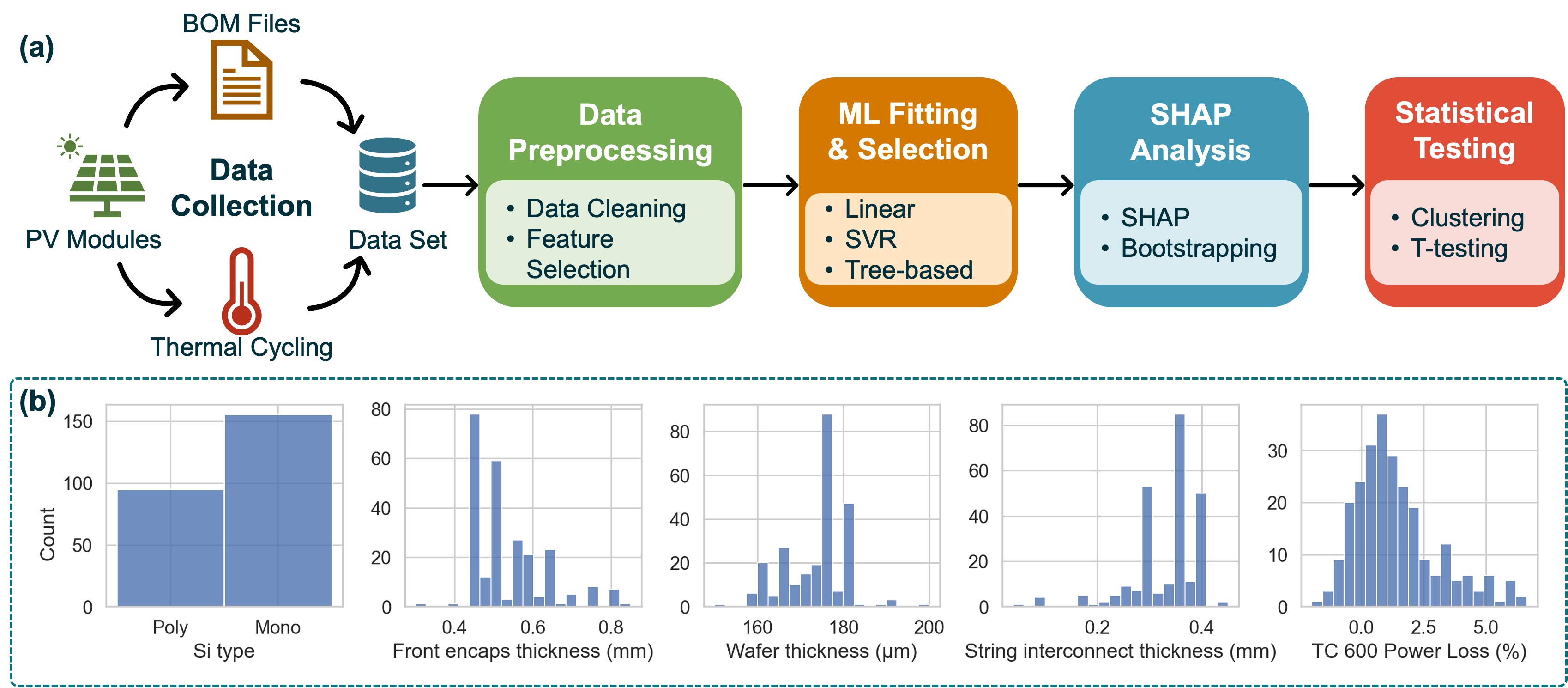
Figure 2: The workflow of the study and data distribution. (a) The steps performed in this study. The data set is constructed by manually extracting information from BOM files and measuring the power loss under thermal cycling tests. The data set is then cleaned and the corresponding features are selected to build machine learning models. Multiple models are fitted and compared, and the final SHAP analysis is conducted based on the best-performing model. (b) Distribution of the selected feature values and the power loss of each module. The distribution of other features is shown in the SI.

II-A BOM Data Collection

275 solar modules of different designs were collected from 47 different manufacturers by PVEL. Those modules are estimated to cover around 70% various types of designs in the market by the date of collection. The BOM data were extracted manually from the document files provided by those manufacturers and yielded over 100 features, including supplier information, dimensions and configurations, materials of PV components such as cells, connections, encapsulants, backsheets and glasses. In this study, we select certain features that are essential for the machine learning modeling based on the steps as described in the following Section II-C.

II-B Thermal Cycling Test

The thermal cycling test is conducted following the standard outlined in IEC 61215-2:2016 [28]. Each module is placed in an environmental chamber and submitted to cycles of temperatures from $-40^{\circ}\text{C}$ to $+85^{\circ}\text{C}$. Each cycle contains maximum $100^{\circ}\text{C}/\text{hr}$ ramp rate and minimum 10min dwell time. Each complete cycle takes 6 hours. A current-voltage (IV) flash test (Pasan SunSim 3B) is performed at standard test conditions following IEC 60904-1:2006 [29] before the aging test and after every 200 cycles to measure the IV curve of modules.

II-C Data Preprocessing

To construct the data set for machine learning models, we preprocess the raw data by data cleaning and feature selection. Data cleaning includes outlier detection using residual analysis, data type casting, and missing data handling using a k-nearest-neighbor (KNN) imputer [30]. The comprehensive description of those steps is included in the Supporting Information (SI) section titled “Data Preprocessing”. Subsequent to the data cleaning process, we select features from more than 100 BOM attributes in the raw data set. This selection is made to construct the feature matrix (i.e., the input X), primarily guided by domain-specific knowledge which will be illustrated in the following Section III. We also perform exploratory data analysis using a correlation matrix to help select the features. The correlation coefficients among features and the target variable are calculated using the Python package Pingouin [31] and Scipy [32]. Spearman correlation is used between two numerical variables $X$ and $Y$. Analysis of variance (ANOVA) is used to test the statistical association between a numerical variable and a categorical variable. Chi-square is used for two categorical variables. The formulae of those testing are demonstrated in SI Section “Feature Selection”.

II-D ML Models

We develop the ML models using toolkits from the Scikit-learn package [33] to model the correlation between BOM features and the power loss. The XGBoost model is not originally included in Scikit-learn and is constructed using the open-source XGBoost package [34]. The split of the development set, the model evaluation metric and the description of model architectures are illustrated as the following:

II-D1 Data Splitting and Model Evaluation

The data set is split into the training set and the testing set with a splitting ratio of 8:2. The training set is further divided into five parts for 5-fold cross-validation to compare models. In each validation iteration, four parts are used for training and the rest part is used for validation. The performance after cross-validation is the average performance from each iteration. Furthermore, the hold-out testing set is used to evaluate the generalization of the optimal model picked from the cross-validation process. The root mean squared error (RMSE) is selected to evaluate the model performance as defined in Equation 1.

$$RMSE=\sqrt{\frac{1}{n}\sum_{i=1}^{n}{\left(\hat{y}_{i}-y_{i}\right)^{2}}}$$ (1)

where $n$ is the number of data points, $\hat{y}_{i}$ is the prediction for the data point $i$ and $y_{i}$ is the ground truth of $i$.

II-D2 Linear Model

The generalized formula of a linear model follows Equation 2:

$$\mathbf{y}=\mathbf{Xw}$$ (2)

where $\mathbf{y}\in\mathbb{R}^{n}$ is the target vector, $\mathbf{X}\in\mathbb{R}^{n\times d}$ is the feature matrix, and $\mathbf{w}\in\mathbb{R}^{d}$ is the model weight. $n$ is the number of measurements and $d$ is the number of features. The training aims to find the $\mathbf{w}$ that minimizes the loss between the measured values and the predicted values, as shown in Equation 3.

$$\hat{\mathbf{w}}=\operatorname{argmin}_{\mathbf{w}}\|\mathbf{y}-\mathbf{Xw}\|_{2}^{2}+\lambda R$$ (3)

where $\lambda R$ is the regularization term with the hyperparameter $\lambda$ to prevent overfitting. Lasso regression [35] with $L1$ regularization ($\lambda\|\mathbf{w}\|_{1}$) and Ridge regression [36] with $L2$ regularization ($\lambda\|\mathbf{w}\|_{2}^{2}$) were trained in this research. The equations for those regularization terms are shown in the SI Section “ML Modeling”.

II-D3 SVR

Support vector regression [37] finds a hyperplane with margins that minimize the error between the true value and predicted values. The equations for SVR is shown in the SI Section “ML Modeling”.

II-D4 Tree-based Model

Random Forest and XGBoost are trained in this research. Random forest regression builds an ensemble of decision trees on different subsets of the original data using bootstrapping and splits nodes on a random subset of features, which helps to increase robustness and prevent overfitting. The final prediction result is the average of the prediction from each decision tree. XGBoost uses boosting method by building decision trees sequentially, each trained to correct its predecessor’s errors. Both tree-based models can be regularized by limiting the depth of trees or the number of nodes. XGBoost can also be regularized using $L1$ or $L2$ regularization in gradient boosting.

II-E SHAP Analysis

To interpret ML models and understand the correlation between BOM features and power loss, we use SHAP method to explain the ML models and apply bootstrapping to qunatify the uncertainty of this method. The average contributions of each BOM feature represent the feature importance, and the dependence between feature values and SHAP values reflects the feature impacts on the power loss.

II-E1 SHapley Additive exPlanations (SHAP)

SHAP is a model-agnostic method that interprets each feature’s marginal contribution to a specific prediction of the machine learning model. It can interpret both local prediction and global contributions of each feature via the additive method. SHAP measures the marginal contribution by computing the SHAP value of each feature ($\phi_{j}$), defined as:

$$\phi_{j}=\sum_{S\subseteq\{1,\ldots,p\}\backslash\{j\}}\frac{|S|!(p-|S|-1)!}{p!}(\text{Val}(S\cup\{j\})-\text{Val}(S))$$ (4)

where $S$ is a subset of the features used in the model, and $p$ is the number of features. $\{1,\ldots,p\}\backslash\{j\}$ represents the set without feature $j$. $\text{Val}(S)$ is the prediction for feature values in set $S$ that are marginalized over features not included in set $S$.

A prediction can be interpreted as the sum of SHAP values of each feature, as shown in Equation 5, where $\hat{f}(x)$ is the prediction, $E[\hat{f}(x)]$ is the expectation of the prediction, $\phi_{j}$ is the SHAP value (i.e., contribution) of the feature $j$. The detailed explanation of how to interpret the SHAP values will be illustrated in Section III.

$$\hat{f}(x)=E[\hat{f}(x)]+\sum_{j=1}^{p}\phi_{j}$$ (5)

II-E2 Bootstrapping

The uncertainty of the Shapley value is determined by using Bootstrapping [38], which randomly sampled with replacement from the original data set 1,000 times and SHAP values of each feature are computed in each iteration. This results in the distribution of the SHAP value of each feature. The confidence interval (CI) of the Shapley value is quantified by using a 95% confidence level.

II-F Post-hoc Statistical Analysis

We conduct post-hoc statistical testing on the original data set to validate the SHAP interpretation of our ML models. The steps include re-grouping the original data set to generate control groups using clustering and a subsequent statistical testing.

II-F1 Clustering

K-means [39] implemented with Scikit-learn is used to do the clustering, which partitions data into a predefined number of clusters (K) by iteratively assigning each data point to the nearest centroid and then recalculating the centroids as the mean of all points in the cluster until the centroids stabilize or a maximum number of iterations is reached. Before clustering, the feature matrixiswas standardized following Equation 6 and weights are assigned to each feature based on their importance following Equation 7

$$Z=\frac{X-\mu}{\sigma}$$ (6)

where $Z$ is the standardized feature matrix, $X$ is the training feature matrix, $\mu$ and $\sigma$ are the training samples’ mean and standard deviation.

$$\text{feature}_{i}^{*}=\text{feature}_{i}\times\frac{\text{SHAP}_{i}}{\sum_{j}{\text{SHAP}_{j}}}$$ (7)

where $\text{feature}_{i}$ is the standardized value of feature $i$ and $\text{SHAP}_{i}$ is the mean absolute Shapley value of feature $i$.

II-F2 T-test

T-test is conducted using the Pingouin package [31]. The t-value regarding group $a$ and $b$ is defined in SI Section “Post-hoc Statistical Analysis”.

III Results and Discussion

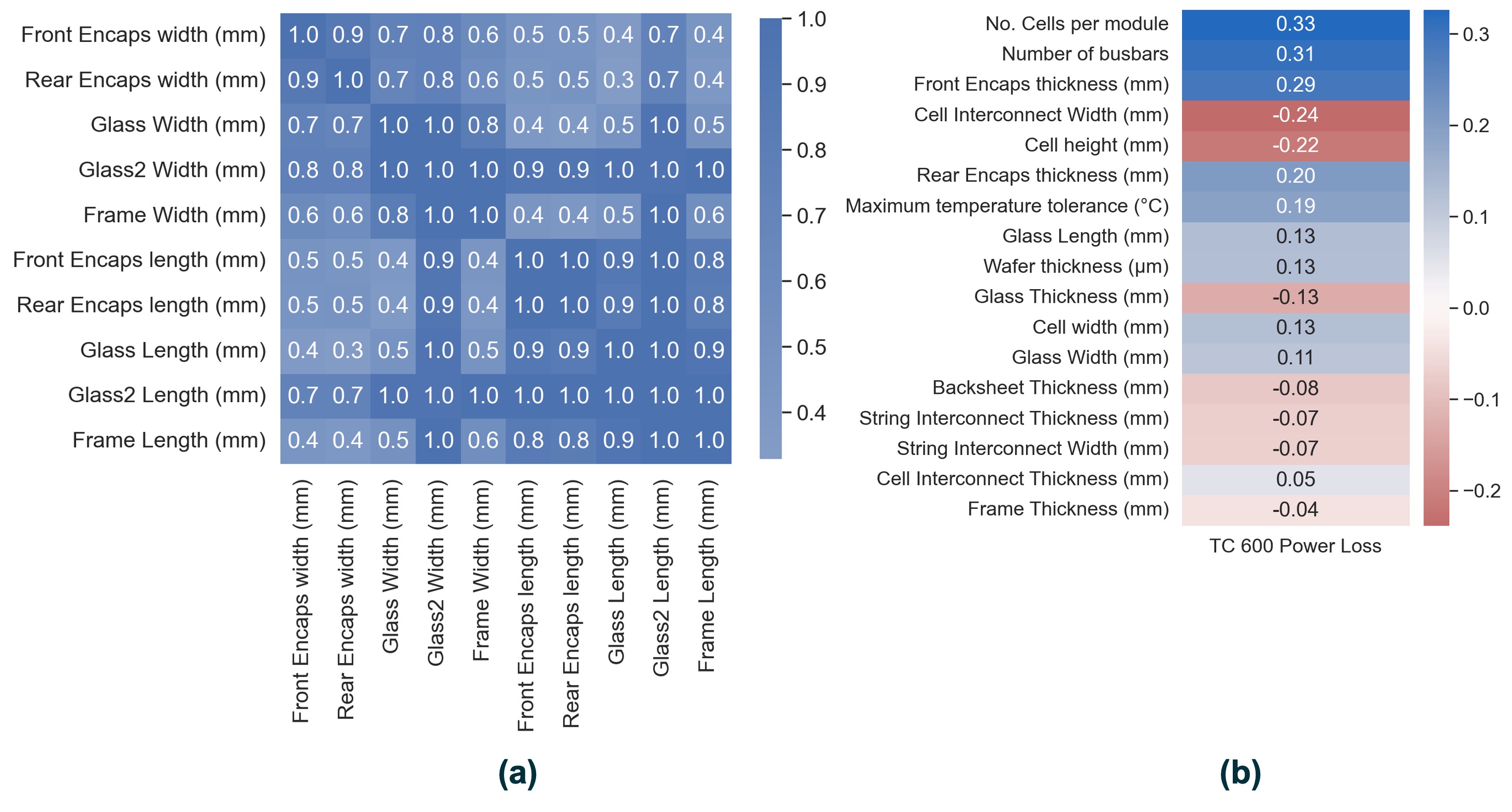
Figure 3: The Spearman correlation between numerical features and the target variable is calculated to assist the construction of the feature matrix in combination with domain knowledge. The correlations shown here are solely used as a reference for feature selection and do not necessarily reflect the true correlations or importance since multiple variables may be entangled. (a) Correlation matrix of numerical features related to module dimensions. (b) Spearman correlation score between selected features and power loss. Features with high correlation coefficient such as the number of busbars are used to construct the feature matrix, although they were not explored in some previous analyses [13, 16]. The full correlation matrices of numerical features as well as categorical features are shown in the SI.

III-A Feature Selection

The distribution of some selected BOM features, alongside the power loss after 600 cycles of thermal cycling test (TC 600), are plotted in Figure 2(b). The goal of feature selection is to identify features with potential correlations to the target variable and reduce inter-feature dependencies because high correlation among features makes the interpretation of feature importance less accurate and less stable. According to previous research [13, 15, 16], the features that influence the stress distribution in solar modules include the thickness, width, and length of each layer and the interconnection thickness, so those features are included in the feature matrix. The mechanical properties such as viscoelasticity of the polymer encapsulant may also influence the module durability, but these properties are difficult to track in the BOM data and are not discussed in this work.

Next, we use the Spearman correlation coefficient [40] to further test the multicollinearity among numerical features and the correlation between features and power loss. Figure 3(a) shows some highly dependent features related to module dimensions, so those features apart from glass length and width are excluded from the feature matrix. Furthermore, we select features that may not be explored in previous regression analyses [9, 13, 16] but still show correlation with thermal cycling degradation based on the correlation matrix in Figure 3(b). For example, the number of busbars was not considered in the previous simulation [13] to save computation time but we still include this feature in our models because this feature shows high Spearman correlation in this data exploration process. It should be noted that Spearman correlation is applicable to numerical variables. Regarding other types of variables, we use the Chi-square test [40] to test the statistical association among categorical features, and Analysis of Variance (ANOVA) [40] to test the statistical association between numerical features and categorical features as detailed in Section II and SI Section “Feature Selection”. We note that the dependence computed here are solely used to help construct the feature matrix and do not necessarily reflect the true correlation between features and power loss due to the interaction of features. Therefore, further analysis like statistical analysis or machine learning modeling is required to determine the correlations or feature importance.

The data preprocessing step removes 24 modules that do not have TC 600 power loss data or have large residuals (over 97% quantile) in the residual analysis as shown in SI. The final feature matrix $\mathbf{X}$ we constructed contains 251 modules with 22 BOM feature columns and the target variable $\mathbf{Y}$ is the power loss (%) after 600 thermal cycles as defined in Equation 8.

$$\Delta P(\%)=\frac{P^{max}_{init}-P^{max}_{after}}{P^{max}_{init}}\times 100\%$$ (8)

where $P_{init}^{max}$ is the module’s maximum output power before the aging test and $P_{after}^{max}$ is the maximum output power after 600 thermal cycling test. The complete distribution of the 22 features can be found in the SI Section “Feature Selection”.

III-B ML Modelling

TABLE I: Mean value and standard deviation of RMSE of each model during the 5-fold cross validation.

Model	RMSE_mean	RMSE_std
Lasso (Linear)	1.614	0.156
Ridge (Linear)	1.631	0.159
SVR	1.657	0.195
RF (Tree-based)	1.427	0.247
XGBoost (Tree-based)	1.491	0.133

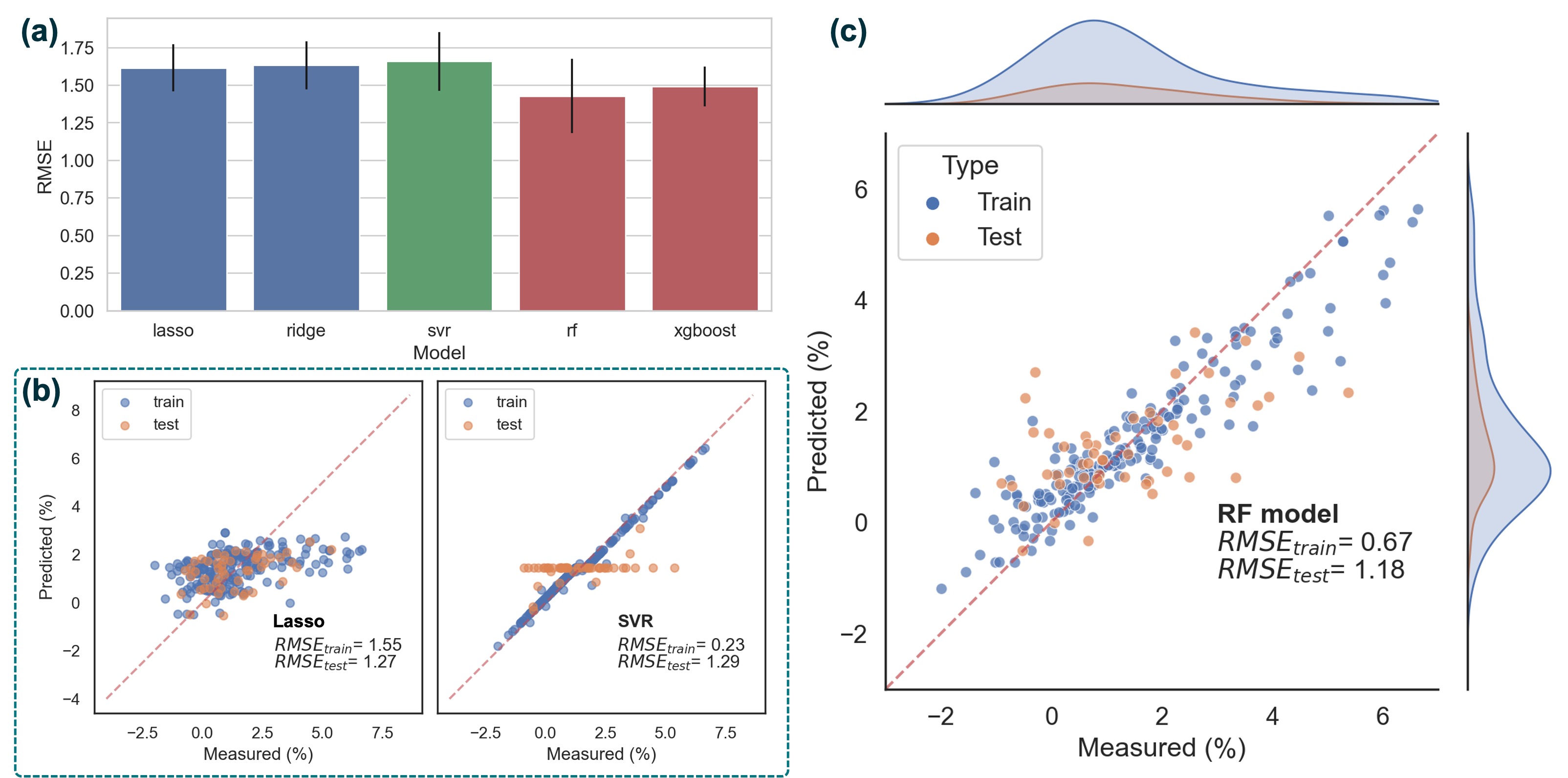
Figure 4: Comparison of machine learning models and generalization test of the optimal model. (a) The 5-fold cross-validation RMSE score for each model. The error bar shows the standard deviation of scores in each fold. Tree-based models (RF and XGBoost) present the best performance. (b) The performance of the Lasso and SVR on the training and testing set, which present underfitting and overfitting. (c) The performance of the selected RF model on the hold-out testing set. Relatively low testing RMSE compared to the training score shows that the RF model is not severely overfitted and generalized well on the new data set.

Next, we train and compare multiple regression models, including linear (Lasso and ridge regression), support vector regression and tree-based (RF and XGBoost) models to find the model that minimizes prediction error. The linear models act as the baseline for model comparison. We use k-fold ($k=5$) cross-validation to test the robustness of models with 80% of the data set (i.e., training set). The hyperparameters of those models are tuned using grid search, as described in the SI. In all cases the model performance is assessed using root mean square error (RMSE) between the measured values and the predicted values. Table I and Figure 4(a) compares the mean value and standard deviation of RMSE of each model during the 5-fold cross-validation. To mitigate the influence of large difference between feature ranges on the linear models, especially when those features have different units, we also train the linear models on a standardized data set following the standardization equation (Equation 6). However the linear model performance is not varied (details included in SI). We note that tree-based models are not influenced by this difference between feature ranges and do not require standardized data set. Overall, the tree-based models outperform other models, with validation RMSE of $1.427(\pm 0.247)$ for RF and $1.491(\pm 0.133)$ for XGBoost. This is unsurprising because linear models do not capture the nonlinear relationships between the BOM features and the power loss, and SVR tends to develop severe overfitting as shown in Figure 4(b). Considering the low mean error and simpler implementation, we selected RF as the optimal model for the subsequent SHAP analysis. It should be noted that although the difference in RMSE values between tree-based models and other models may seem marginal in Table I, given the low target variable values, even minor RMSE variations can signify substantial prediction performance disparities. This significant difference in performance among models can be visualized in the scatter plots of predicted values vs. measured values. For example, the plot for Lasso model in Figure 4(b) clearly shows underfitting since the scatter points are not distributing along the “Measured=Predicted” line (the diagonal dash line). The scatter plots of all the models are demonstrated in the SI Section “ML Modeling”.

We further test the generalization of the RF model on the hold-out 20% of the data set (i.e., testing set), as shown in Figure 4(c). The RMSE of the hold-out testing data (1.179) is not drastically higher than the training error, as opposed to the overfitted SVR model. This indicates that the fitted RF model is able to capture the underlying correlation between the BOM data and the degradation and has generalization on new data. Following model selection, we retrain the optimal RF model on the combined data set (i.e., training and testing set), achieving a RMSE of 0.558, and proceed to interpret this model using the SHAP method.

III-C SHAP Analysis of BOM Impacts

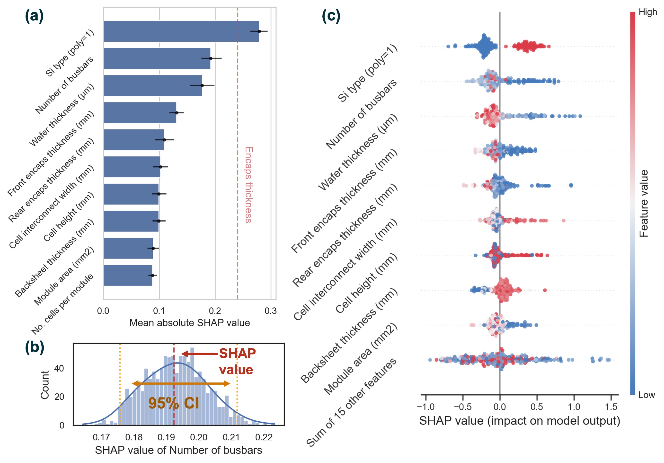
Figure 5: SHAP interpretation of the machine learning model and uncertainty determination. (a) The feature importance rank of the BOM features. The mean absolute SHAP value is calculated over all the modules in the original data set. The error bar shows the uncertainty with 95% confidence level using bootstrapping (random sampling from the original data set). The red dash line shows the sum of SHAP values of both front and rear encapsulant thickness, indicating that the encapsulant thickness is also a very important feature other than the Si type. (b) An example of the bootstrapping distribution of the number of busbars using 1000 sampling. (c) The beeswarm plot of SHAP values. It shows the dependent relation between each feature and the power loss. The color of each point denotes the feature values. Red color denotes a larger feature value and blue color denotes a smaller feature. The x-axis is the SHAP value (i.e., impact on degradation) of each feature. For example, a blue cluster of points with a positive SHAP value means a lower feature value tends to increase the power loss.

To interpret the random forest model, we use the SHAP method to investigate the importance of features and the relation between features and power loss. SHAP analysis reveals the impact of a certain feature on the model prediction while marginalizing the effect of other features. A prediction (i.e., power loss) of the model can be considered as the sum of the contributions of each BOM feature (i.e., SHAP values). The features that comprise the highest portion of power loss on average are considered the most important features. Figure 5(a) shows the average impact of each feature on the prediction based on the SHAP values, computed with the aforementioned RF model. Specifically, Figure 5(a) arranges the top ten important BOM features from top to bottom in the order of decreasing mean absolute SHAP values (i.e., feature importance). The average is calculated over each module in the original data set. To determine the uncertainty of the feature importance, we repeatedly run a 1,000 iteration bootstrapping by sampling subset from the original data set and compute corresponding mean absolute SHAP values. We select a 95% confidence interval, shown as the error bars in Figure 5(a), to quantify the uncertainty. The interval indicates the robustness of this method to the random selection in the training data. Figure 5(b) shows an example of the bootstrapping distribution of the SHAP value of the “Number of busbars”, which follows a normal distribution consistent with the central limit theorem [40]. The SHAP value computed from the original data is indicated by the red dash line and the boundaries of the 95% CI computed from the bootstrapping are indicated by the orange dash line.

In addition, Figure 5(c) depicts a beeswarm plot, with each dot representing the SHAP value of each feature in each measurement. Red color denotes a larger feature value and blue color denotes a smaller feature value. Due to the additive property of the SHAP formula shown in Section II, the power loss of a module can be considered as the sum of SHAP values of each feature, and thus the dependence between the SHAP value and the feature value reflects the relation between the power loss and the BOM feature. For example, in Figure 5(c), the blue dots (lower feature value) in the “Front encaps thickness (mm)” row with positive increasing SHAP values (higher power loss) suggest that lower front encapsulant thickness tends to increase the power loss.

To better visualize this dependence, we also construct Figure 6 to illustrate the relationship between the SHAP values and their corresponding feature values, which reflects the impacts of features on the power loss. Figure 6(a)-(d) shows the dependence plot of the top five important features besides the Si type and Figure 6(e)(f) demonstrate two features that were investigated in the previous studies [9, 13]. In these dependence plots, the mean SHAP value corresponding to each feature value is displayed as one dot and the standard deviation is used for the error bar. The bottom rug plot in each sub-figure shows the distribution of the data. A smooth spline interpretation with 95% prediction interval is used to illustrate the trend of the relationship.

In general, Figure 5 demonstrates that “Si type (poly=1)”, which represents whether the solar cell is mono-c (denoted as 0) or poly-c (denoted as 1) Si, is listed as the most important feature. Also this feature still remains the most important even when the lower bound of the confidence interval is considered. This indicates that the Si type is the predominant design factor that impacts the thermal cycling power loss. The subsequent influential features are “Number of busbars”, “Wafer thickness”, “Front encaps thickness” and “Rear encaps thickness”. If we consider the thickness of the front and rear encapsulant together due to their similarity and add up their SHAP values, the encapsulant thickness is the next important BOM feature other than the Si type as shown in the red dash line in Figure 5(a). It should be noted that Si type and encapsulant thickness are the two top important features with robustness, but the importance rank of other features can vary according to the confidence interval in Figure 5(a). The detailed interpretation of the impacts of these features will be discussed in the subsequent paragraphs. The SHAP values of the rest features are not significant ($<0.1$) compared to these primary ones and are not discussed in detail in this paper.

III-C1 Impact of Si type

Based on the SHAP interpretation, Si type is the predominant design factor regarding the module’s thermomechanical durability. Specifically, Figure 5(c) shows that poly-c Si modules possess positive SHAP values, implying a tendency towards higher power loss for such modules. To the best of our knowledge, this difference in durability between mono-c and poly-c Si modules was not reported previously. Since mono-c and poly-c Si have similar CTE [41], the variance of power loss may not be caused by the difference in thermal expansion. One plausible reason involves the grain boundary in poly-c Si serving as initiation sites of micro-cracks [42]. These micro-cracks can propagate with successive thermal cycle, leading to a degradation in the performance of the solar module over time even before the crack length reaches the threshold of a catastrophic breakage. We note that the impact of micro-cracks on module electric power and the evolution of micro-cracks in long-term cyclic loading remains a topic of ongoing research [2, 43, 44], so other factors may also cause the difference in the power loss here. Another possible reason is that the current data set may be influenced by other confounding variables. The mitigation of the influence of confounding variables will be illustrated in the following subsection “Statistical Validation of SHAP Interpretation”.

III-C2 Impact of encapsulant thickness

The encapsulant thickness remains another important design factor. From Figure 6(a)(b), both front and rear encapsulant thickness exhibit negative dependence with increasing thickness when the thickness is lower than around $0.6-0.7\text{mm}$, suggesting that thicker encapsulant might result in lower power loss. This corresponds to previously simulated results [13] that thicker encapsulant decreases the accumulated thermal stress in the solder layer. Also, as a soft embedding of the Silicon solar cells, the encapsulant can compensate for the strain coming from the glass during deflection [45]. Interestingly, when the front encapsulant thickness is larger than $0.7\text{mm}$, the power loss is increased, especially for the front encapsulant. This opposite trend was not reported by previous regression analysis [9, 13]. A possible cause for this trend is a change of mechanical property of the polymer at lower temperature. At high temperature, the encapsulant layer is soft and acts as a compensation layer for the strain difference between the glass and Si layer. However, lower temperature, especially approaching or below the glass transition temperature ($\sim-33^{\circ}\text{C}$ [46] for EVA and $\sim-25^{\circ}\text{C}$ [47] for POE), limits the mobility of polymer chains and thus increases the stiffness of the encapsulant. This transition transforms the laminated structure of solar module into so-called glass-encapsulant-Si “sandwich” structure and more strain is conducted to the cell layer by the stiff encapsulant as the module bends during thermal cycling [45, 48]. In this structure at low temperature, thicker encapsulant between the glass and Si layer, which is the front encapsulant, can increase the tensile stress in the Si layer and lead to higher Si fracture probability. Such a phenomenon was previously reported by Dietrich et al. [45] that, at $-40^{\circ}\text{C}$, thicker encapsulant leads to higher probability of failure. Therefore, in our BOM data set, the power loss first decreased with thicker encapsulant and then increased as the failure at lower temperature dominates. The hypothesis here can also explain that front encapsulant presents steeper increase at tail region ($>0.7\text{mm}$) in Figure 6(a) than the rear encapsulant in Figure 6(b) since the front encapsulant locates between the glass and Si layer conduct more strain. However, we note that since the measurements at the tail region are sparse, this trend of increase may also be influenced by noise. Further testing with more controlled data sets may be needed to validate the hypothesis.

III-C3 Impact of busbar number

Figure 6(c) demonstrates that the power loss decreases as the number of busbars increases to around 7 and then increases with more busbars soldered on solar cells. This is reasonable because increasing the number of busbars can increase the probability of current connection between cells and external circuits even when the solder layer beneath some busbars got cracked due to thermal stress. However, too many busbars soldered on the Si wafer can yield more residual thermal stress during the fabrication process, which causes solder disconnection and even wafer fracture during operation [49, 50]. We believe this to be the origin of why the power loss is reduced when the number of busbars increases in the beginning, and then increases with more busbars soldered. We also notice the drop of SHAP value at 12 busbars but since the measurements are sparse so it cannot represent the general trend of impacts.

III-C4 Impact of wafer thickness

The wafer thickness was considered as a top important factor in previous studies [9, 13] and also remains an important feature in our data set. However, the impact of wafer thickness in our real-world data set shows a different trend to previously simulated results. Figure 6(d) indicates that a thinner wafer thickness ($<180\text{{\textmu}m}$) can increase power loss, contrary to previous studies that recommended thinner wafers. However, when the thickness is greater than $180\text{{\textmu}m}$, thinner wafer is beneficial for durability. This discrepancy may arise because earlier simulations primarily focused on damage within the solder layer. However, the silicon wafer, as a brittle material, is more likely to experience catastrophic fracture if the thickness is excessively reduced. This potentially offsets the advantages of reduced damage in the solder layer. This trend aligns with another study that higher wafer thickness is important in the module design [16].

III-C5 Impact of other features

Furthermore, Figure 6(e) and (f) demonstrate the impacts of the cell interconnection (i.e., copper ribbon) thickness and backsheet thickness, which were explored in the previous simulations [9, 13]. From Figure 6(e), it can be seen that modules with lower ribbon thickness have lower power loss because of lower thermal stress in the solder layer [9]. However, we consider this trend to be unreliable because the data points at region over $0.35\text{mm}$ and lower than $0.20\text{mm}$ are sparse and may skew this trend. Figure 6(f) suggests that the power loss is expected to increase as the backsheet thickness increases. This increase corresponds to the conclusion from the previous investigation [13] that thicker backsheet leads to more accumulated damage in the solder layer.

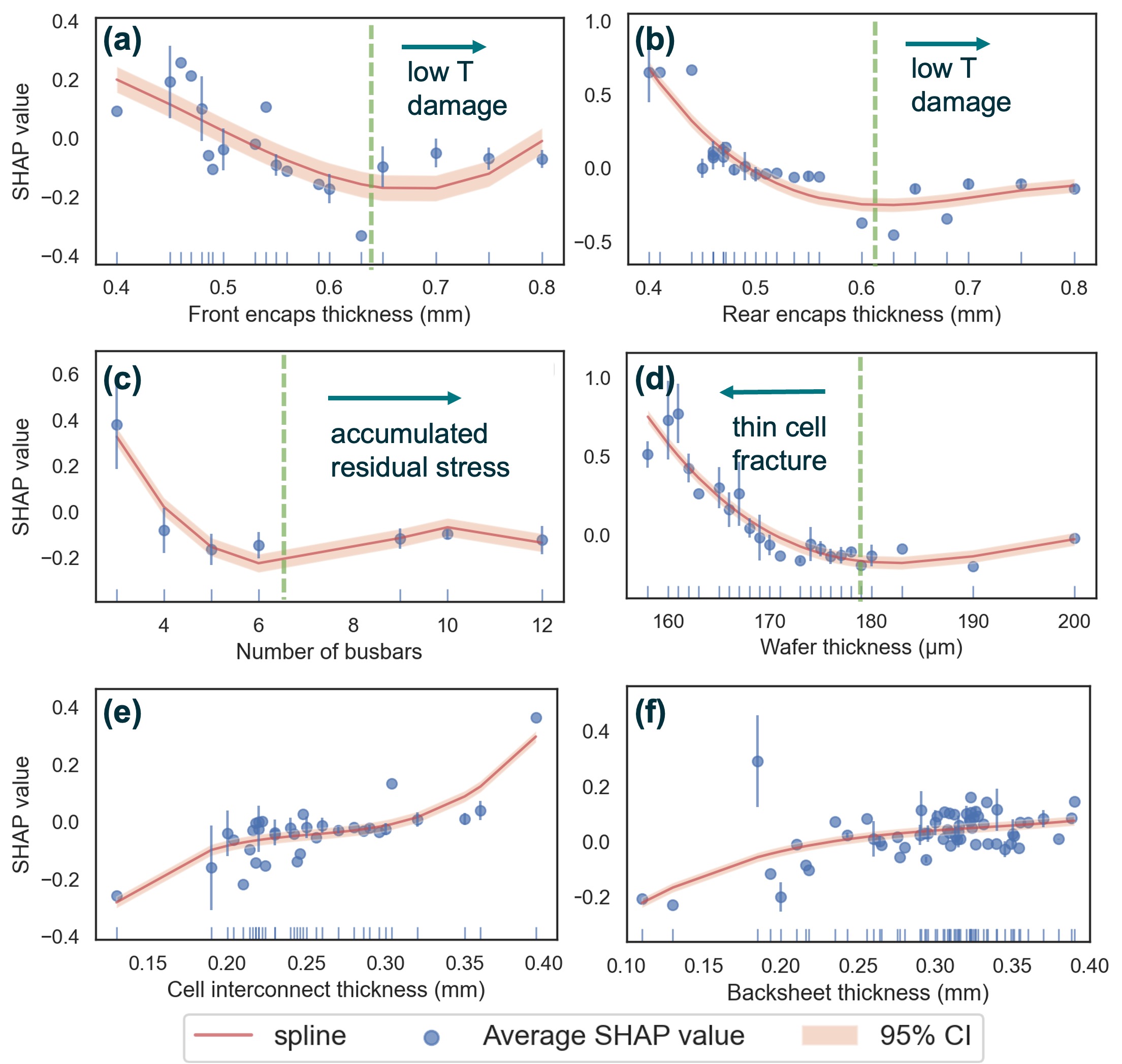
Figure 6: Dependence plot of the relation between numerical features and SHAP value. Due to the additive property of the SHAP formula, the SHAP value is related to the power loss so the dependence plot also reflects the relation between the power loss and the BOM features. The bottom rug plot in each sub-figure shows the distribution of the data. (a)-(d) shows the relation of the top five features apart from the Si cell type. (e) and (f) examine the impact of the two features that were considered in the previous literature.

III-D Statistical Validation of SHAP Interpretation

Utilizing SHAP analysis allows us to understand the most influential BOM features and their impacts on power loss. However, the validity of SHAP interpretation is contingent upon the performance of the machine learning models, necessitating supplementary investigations. Herein, we conduct an independent post-hoc statistical testing on a controlled subset derived from the original data set to determine whether Si type is indeed impactful. We construct this subset using clustering method so that feature values in this subset are similar apart from the Si type to counteract the confounding variables. We note that we select the Si type for this analysis because not only is it the most impactful factor, but it is a categorical variable which makes the control process easier. The example of clustering other numerical features is included in the SI Section “Post-hoc Statistical Analysis”, which shows that the control group is hard to obtain for other variables.

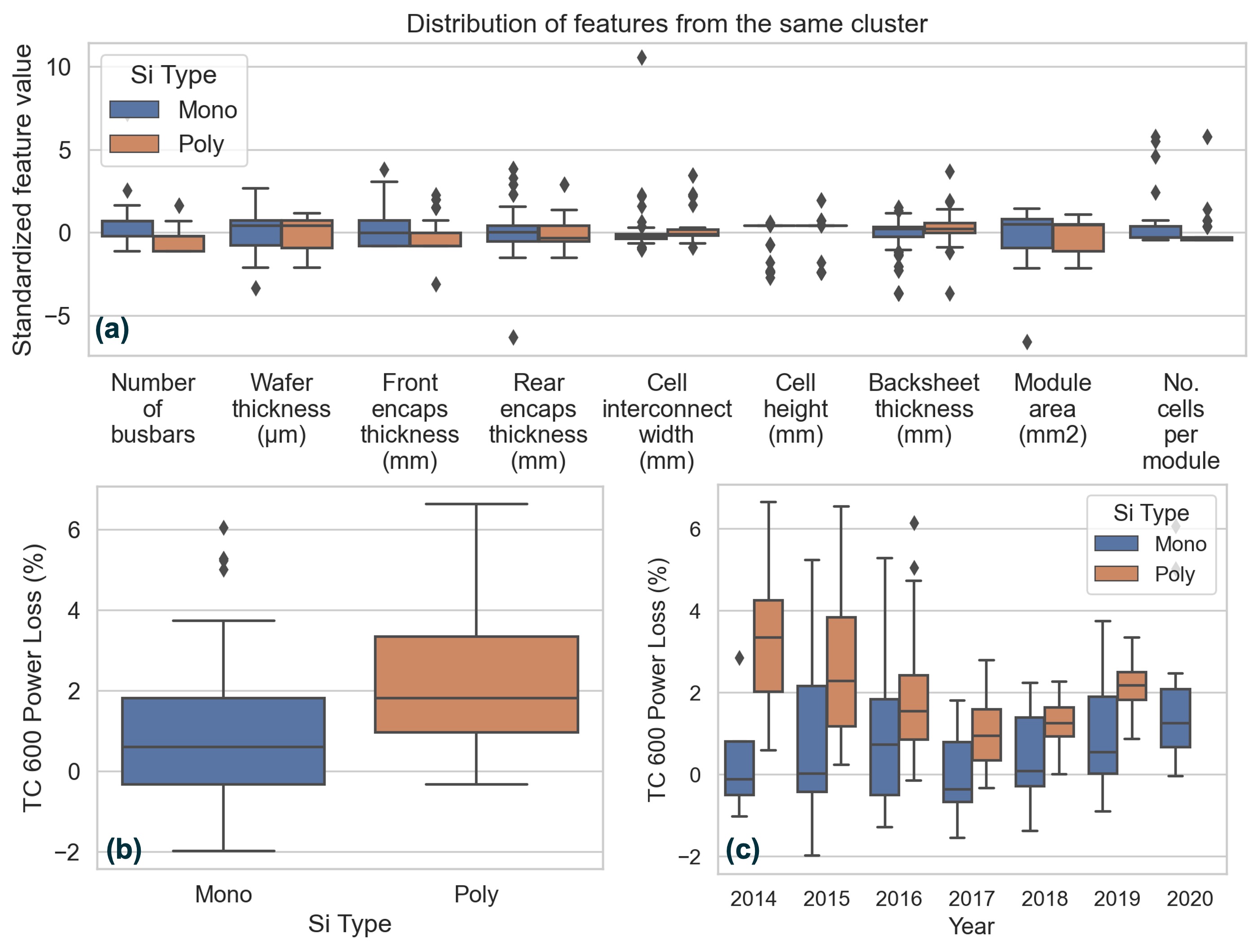
Figure 7: Statistical testing to verify the impact of the Si cell type. Sample data is first extracted from the raw data set using the clustering method to guarantee that features other than Si cell type are randomized. Then t-test is used to test the statistical significance of the Si cell type impact. (a) The distribution of several top important features in the same cluster. The similar distribution comparison between mono-c Si cells and poly-c Si cells indicates the randomization of those features. (b) The distribution of power loss between mono-c Si cells and poly-c Si cells in the same cluster. The p-value smaller than 5% indicates that poly-c Si modules have a statistically significant increase in the thermal cycling power loss. (c) The distribution of Si type in each year. The higher power loss of poly-c Si modules indicates that the manufacturing year is not the confounding variable.

To construct this subset, we perform k-means clustering on the original data set, neglecting the Si type in the clustering process, to gather measurements with similar feature values besides Si type. We use the “elbow” method to determine the optimal number of clusters to be used and select “$\text{number of clusters}=2$”. We note that the selection of this number is subjective and other values may be also feasible as long as BOM features other than Si type can be randomized in the same cluster. In the next step, we pick up the subset (i.e., cluster) for further testing with the greatest number of data points. The related details of clustering are included in the SI Section “Post-hoc Statistical Analysis”, After clustering, the distribution of the top ten important BOM features other than Si type is shown in Figure 7(a). It can be seen that the boxplot of most features for those cells are similar but contain differences in Si type, which means those features are randomized between mono-c and poly-c Si. In addition, we check the normality of the power loss for both types of cells in this cluster, which is prerequisite for further parametric statistical testing. Here we use the Quantile-quantile (Q-Q) plots to check normality, which are included in SI.

With all the prerequisite processing of the data set, we conduct a t-test to compare the mean power loss of poly-c Si modules and mono-c Si modules from the same cluster. Figure 7(b) compares the distribution of power loss of mono-c and poly-c Si modules from the selected cluster, which displays that poly-c Si modules have more power loss on average. The null hypothesis of our t-test is:

$$\mathbf{H_{0}}:\textit{Poly-c Si modules don't exhibit higher thermal cycling power loss than mono-c Si modules.}$$

The testing result illustrates that the power loss of poly-c Si modules is higher than that of mono-c Si modules and this result is statistically significant ($\text{p-value}=1.4\times 10^{-8}<5\%$). This validates the interpretation of SHAP analysis.

Although the clustering can mitigate the influence of uncontrolled variables, some other variables that are not included in the ML modeling may still impact our interpretation. One of the most potential confounding variables is the manufacturing process. To mitigate the influence of different suppliers, this dataset analyzes modules from various manufacturers. Also in Figure 7(c), we compare the power loss of the two types of modules from the same cluster in each manufacturing year. It reveals that poly-c Si modules still have higher power loss each year, which means the manufacturing year is not the underlying reason for the difference. Despite these efforts, there is still a chance that some unrecorded manufacturing conditions during the fabrication of poly-c and mono-c Si modules may vary and influence the thermomechanical durability rather than the Si type itself. As in all such cases, data analysis can point the direction to highly plausible hypotheses, but careful and dedicated experiments would be needed to confirm each trend.

IV Conclusion

In this study, we determine the most influential BOM features in the current module design and investigated their impacts on thermomechanical durability based on a unique data set by collecting full-size modules from various manufacturers. We correlate the BOM features with the thermal cycling power loss after 600 cycles by fitting machine learning models. We compare the performance of several models including linear, SVR and tree-based models, and select the Random Forest (RF) model with a testing RMSE of 1.179 as the optimal model and a RMSE of 0.558 on the whole data set for further SHAP interpretation. We subsequently apply SHAP analysis with the fitted RF model to interpret the whole data set and used statistical testing to verify the conclusion.

Overall, we find that the Si type (i.e., whether the module is composed of poly-c or mono-c Si cells) is the most influential factor. We conduct k-means clustering and t-test to verify that poly-c Si modules have higher power loss. We speculate that this is due to crack initialization at grain boundaries during the cycling; however, further experiment is required to support this hypothesis. We note that the solar industry is phasing down the usage of poly-c Si cells. The findings from this analysis can provide another motivation for the switch from poly-c to mono-c Si cells. The next most important feature is the thickness of both the front and rear encapsulant; a higher thickness can reduce power loss, but further increases of the thickness (particularly for the front encapsulant) shows an opposite impact.

We also analyze the impacts of other features. Notably, we find that increasing the number of busbars initially reduces power loss, but subsequently increases it. This should raise attention because the multi-busbar design is becoming prevalent in the recent module manufacturing, but their long-term durability remains in need of further study  [51]. The wafer thickness displays an opposite trend to previous findings [9, 13]. In our data set, too low wafer thickness is not beneficial to the durability, probably because a thinner Si wafer is less robust to fracture. We further find that the power loss is dropped when the ribbon thickness is decreased and thinner backsheet layer is beneficial for durability.

Finally, it is important to acknowledge the limitations of our study. Although our data set covers a breadth of BOM features, certain areas like the solder thickness or various CTEs of encapsulants, remained uncharted due to the difficulty of tracking this information from manufacturers. Furthermore, the use of commercially available modules as opposed to carefully controlled modules means that conclusions might still be influenced by confounding variables, underscoring the need for further investigation. Despite these constraints, we hope this study can reveal the potential application of machine learning and model-agnostic interpretation methods in examining BOM effects on reliability and provide insights into the direction of future module optimization.

V Data Availability

The data set is available at DuraMat Datahub (https://datahub.duramat.org/dataset/bom_thermal_cycling_degradation). Some values in the published data set are redacted according to non-disclosure agreement.

VI Code Availability

Our codes for ML modeling and SHAP interpretation are available at Github repository(https://github.com/DuraMAT/bom_analysis).

Declaration of Generative AI and AI-assisted technologies in the writing process

During the preparation of this work the author(s) used Writefull & Chatgpt in order to check grammar and improve readability. The author(s) did not use this tool/service to directly generate the manuscript but only to polish the manuscript written by the author(s). After using this tool/service, the author(s) reviewed and edited the content as needed and take(s) full responsibility for the content of the publication.

References

- [1] K. Ardani, P. Denholm, T. Mai, R. Margolis, E. O’Shaughnessy, T. Silverman, and J. Zuboy, “Solar futures study,” U.S. Department of Energy, Tech. Rep., 2021.
- [2] M. Aghaei, A. Fairbrother, A. Gok, S. Ahmad, S. Kazim, K. Lobato, G. Oreski, A. Reinders, J. Schmitz, M. Theelen et al., “Review of degradation and failure phenomena in photovoltaic modules,” Renewable and Sustainable Energy Reviews, vol. 159, p. 112160, 2022.
- [3] D. C. Jordan, T. J. Silverman, J. H. Wohlgemuth, S. R. Kurtz, and K. T. VanSant, “Photovoltaic failure and degradation modes,” Progress in Photovoltaics: Research and Applications, vol. 25, no. 4, pp. 318–326, 2017.
- [4] S. Kawai, T. Tanahashi, Y. Fukumoto, F. Tamai, A. Masuda, and M. Kondo, “Causes of degradation identified by the extended thermal cycling test on commercially available crystalline silicon photovoltaic modules,” IEEE Journal of Photovoltaics, vol. 7, no. 6, pp. 1511–1518, 2017.
- [5] U. Eitner, M. Köntges, and R. Brendel, “Use of digital image correlation technique to determine thermomechanical deformations in photovoltaic laminates: Measurements and accuracy,” Solar Energy Materials and Solar Cells, vol. 94, no. 8, pp. 1346–1351, 2010.
- [6] C. Borri, M. Gagliardi, and M. Paggi, “Fatigue crack growth in silicon solar cells and hysteretic behaviour of busbars,” Solar Energy Materials and Solar Cells, vol. 181, pp. 21–29, 2018.
- [7] S. Wiese, R. Meier, and F. Kraemer, “Mechanical behaviour and fatigue of copper ribbons used as solar cell interconnectors,” in 2010 11th International Thermal, Mechanical & Multi-Physics Simulation, and Experiments in Microelectronics and Microsystems (EuroSimE). IEEE, 2010, pp. 1–5.
- [8] T. J. Silverman, M. Bliss, A. Abbas, T. Betts, M. Walls, and I. Repins, “Movement of cracked silicon solar cells during module temperature changes,” in 2019 IEEE 46th Photovoltaic Specialists Conference (PVSC). IEEE, 2019, pp. 1517–1520.
- [9] S. Park and C. Han, “Reliability-driven design optimization of si solar module under thermal cycling,” Journal of Mechanical Science and Technology, vol. 36, no. 8, pp. 4099–4114, 2022.
- [10] J.-S. Jeong, N. Park, and C. Han, “Field failure mechanism study of solder interconnection for crystalline silicon photovoltaic module,” Microelectronics Reliability, vol. 52, no. 9-10, pp. 2326–2330, 2012.
- [11] U. Itoh, M. Yoshida, H. Tokuhisa, K. Takeuchi, and Y. Takemura, “Solder joint failure modes in the conventional crystalline si module,” Energy Procedia, vol. 55, pp. 464–468, 2014.
- [12] H. Hanifi, M. Pander, U. Zeller, K. Ilse, D. Dassler, M. Mirza, M. A. Bahattab, B. Jaeckel, C. Hagendorf, M. Ebert et al., “Loss analysis and optimization of pv module components and design to achieve higher energy yield and longer service life in desert regions,” Applied energy, vol. 280, p. 116028, 2020.
- [13] N. Bosco, T. J. Silverman, and S. Kurtz, “The influence of pv module materials and design on solder joint thermal fatigue durability,” IEEE Journal of Photovoltaics, vol. 6, no. 6, pp. 1407–1412, 2016.
- [14] J. Zhu, M. Owen-Bellini, D. Montiel-Chicharro, T. R. Betts, and R. Gottschalg, “Effect of viscoelasticity of ethylene vinyl acetate encapsulants on photovoltaic module solder joint degradation due to thermomechanical fatigue,” Japanese Journal of Applied Physics, vol. 57, no. 8S3, p. 08RG03, 2018.
- [15] A. J. Beinert, P. Romer, M. Heinrich, M. Mittag, J. Aktaa, and D. H. Neuhaus, “The effect of cell and module dimensions on thermomechanical stress in pv modules,” IEEE Journal of Photovoltaics, vol. 10, no. 1, pp. 70–77, 2019.
- [16] A. J. Beinert, P. Romer, M. Heinrich, J. Aktaa, and H. Neuhaus, “Thermomechanical design rules for photovoltaic modules,” Progress in Photovoltaics: Research and Applications, 2022.
- [17] J. H. Friedman, “Greedy function approximation: a gradient boosting machine,” Annals of statistics, pp. 1189–1232, 2001.
- [18] M. T. Ribeiro, S. Singh, and C. Guestrin, “” why should i trust you?” explaining the predictions of any classifier,” in Proceedings of the 22nd ACM SIGKDD international conference on knowledge discovery and data mining, 2016, pp. 1135–1144.
- [19] S. M. Lundberg and S.-I. Lee, “A unified approach to interpreting model predictions,” Advances in neural information processing systems, vol. 30, 2017.
- [20] P. Bannigan, Z. Bao, R. J. Hickman, M. Aldeghi, F. Häse, A. Aspuru-Guzik, and C. Allen, “Machine learning models to accelerate the design of polymeric long-acting injectables,” Nature communications, vol. 14, no. 1, p. 35, 2023.
- [21] S. A. Giles, D. Sengupta, S. R. Broderick, and K. Rajan, “Machine-learning-based intelligent framework for discovering refractory high-entropy alloys with improved high-temperature yield strength,” npj Computational Materials, vol. 8, no. 1, p. 235, 2022.
- [22] R. Kumar and A. K. Singh, “Chemical hardness-driven interpretable machine learning approach for rapid search of photocatalysts,” npj Computational Materials, vol. 7, no. 1, p. 197, 2021.
- [23] N. T. P. Hartono, J. Thapa, A. Tiihonen, F. Oviedo, C. Batali, J. J. Yoo, Z. Liu, R. Li, D. F. Marrón, M. G. Bawendi et al., “How machine learning can help select capping layers to suppress perovskite degradation,” Nature communications, vol. 11, no. 1, p. 4172, 2020.
- [24] PVEL, “The 2023 pv module reliability scorecard,” 2023. [Online]. Available: https://scorecard.pvel.com/
- [25] T. K. Ho, “Random decision forests,” in Proceedings of 3rd international conference on document analysis and recognition, vol. 1. IEEE, 1995, pp. 278–282.
- [26] Pv evolution labs. [Online]. Available: https://www.pvel.com/
- [27] G. Van Rossum and F. L. Drake, Python 3 Reference Manual. Scotts Valley, CA: CreateSpace, 2009.
- [28] I. E. Commission, “Terrestrial photovoltaic (pv) modules - design qualification and type approval - part 2: Test procedures,” International Electrotechnical Commission, Tech. Rep., 2016.
- [29] ——, “Photovoltaic devices – part 1: Measurement of photovoltaic current-voltage characteristics,” International Electrotechnical Commission, Tech. Rep., 2006.
- [30] O. Troyanskaya, M. Cantor, G. Sherlock, P. Brown, T. Hastie, R. Tibshirani, D. Botstein, and R. B. Altman, “Missing value estimation methods for dna microarrays,” Bioinformatics, vol. 17, no. 6, pp. 520–525, 2001.
- [31] R. Vallat, “Pingouin: statistics in python.” J. Open Source Softw., vol. 3, no. 31, p. 1026, 2018.
- [32] P. Virtanen, R. Gommers, T. E. Oliphant, M. Haberland, T. Reddy, D. Cournapeau, E. Burovski, P. Peterson, W. Weckesser, J. Bright, S. J. van der Walt, M. Brett, J. Wilson, K. J. Millman, N. Mayorov, A. R. J. Nelson, E. Jones, R. Kern, E. Larson, C. J. Carey, İ. Polat, Y. Feng, E. W. Moore, J. VanderPlas, D. Laxalde, J. Perktold, R. Cimrman, I. Henriksen, E. A. Quintero, C. R. Harris, A. M. Archibald, A. H. Ribeiro, F. Pedregosa, P. van Mulbregt, and SciPy 1.0 Contributors, “SciPy 1.0: Fundamental Algorithms for Scientific Computing in Python,” Nature Methods, vol. 17, pp. 261–272, 2020.
- [33] F. Pedregosa, G. Varoquaux, A. Gramfort, V. Michel, B. Thirion, O. Grisel, M. Blondel, P. Prettenhofer, R. Weiss, V. Dubourg, J. Vanderplas, A. Passos, D. Cournapeau, M. Brucher, M. Perrot, and E. Duchesnay, “Scikit-learn: Machine learning in Python,” Journal of Machine Learning Research, vol. 12, pp. 2825–2830, 2011.
- [34] T. Chen and C. Guestrin, “Xgboost: A scalable tree boosting system,” in Proceedings of the 22nd acm sigkdd international conference on knowledge discovery and data mining, 2016, pp. 785–794.
- [35] R. Tibshirani, “Regression shrinkage and selection via the lasso,” Journal of the Royal Statistical Society Series B: Statistical Methodology, vol. 58, no. 1, pp. 267–288, 1996.
- [36] A. E. Hoerl and R. W. Kennard, “Ridge regression: Biased estimation for nonorthogonal problems,” Technometrics, vol. 12, no. 1, pp. 55–67, 1970.
- [37] H. Drucker, C. J. Burges, L. Kaufman, A. Smola, and V. Vapnik, “Support vector regression machines,” Advances in neural information processing systems, vol. 9, 1996.
- [38] B. Efron, “Bootstrap methods: another look at the jackknife,” in Breakthroughs in statistics: Methodology and distribution. Springer, 1992, pp. 569–593.
- [39] J. A. Hartigan and M. A. Wong, “Algorithm as 136: A k-means clustering algorithm,” Journal of the royal statistical society. series c (applied statistics), vol. 28, no. 1, pp. 100–108, 1979.
- [40] P. Bruce, A. Bruce, and P. Gedeck, Practical statistics for data scientists: 50+ essential concepts using R and Python. O’Reilly Media, 2020.
- [41] H. Watanabe, N. Yamada, and M. Okaji, “Linear thermal expansion coefficient of silicon from 293 to 1000 k,” International journal of thermophysics, vol. 25, no. 1, pp. 221–236, 2004.
- [42] P. D. Zavattieri and H. D. Espinosa, “Grain level analysis of crack initiation and propagation in brittle materials,” Acta Materialia, vol. 49, no. 20, pp. 4291–4311, 2001.
- [43] T. J. Silverman, M. G. Deceglie, M. Owen-Bellini, W. B. Hobbs, and C. Libby, “Cracked solar cell performance depends on module temperature,” in 2021 IEEE 48th Photovoltaic Specialists Conference (PVSC). IEEE, 2021, pp. 1691–1692.
- [44] C. Libby, B. Paudyal, X. Chen, W. B. Hobbs, D. Fregosi, and A. Jain, “Analysis of pv module power loss and cell crack effects due to accelerated aging tests and field exposure,” IEEE Journal of Photovoltaics, pp. 1–9, 2022.
- [45] S. Dietrich, M. Sander, M. Pander, and M. Ebert, “Interdependency of mechanical failure rate of encapsulated solar cells and module design parameters,” in Reliability of Photovoltaic Cells, Modules, Components, and Systems V, vol. 8472. SPIE, 2012, pp. 123–131.
- [46] K. Agroui, G. Collins, and J. Farenc, “Measurement of glass transition temperature of crosslinked eva encapsulant by thermal analysis for photovoltaic application,” Renewable Energy, vol. 43, pp. 218–223, 2012.
- [47] M. Baiamonte, C. Colletti, A. Ragonesi, C. Gerardi, and N. T. Dintcheva, “Durability and performance of encapsulant films for bifacial heterojunction photovoltaic modules,” Polymers, vol. 14, no. 5, p. 1052, 2022.
- [48] S. Dietrich, M. Pander, M. Sander, S. H. Schulze, and M. Ebert, “Mechanical and thermomechanical assessment of encapsulated solar cells by finite-element-simulation,” in Reliability of photovoltaic cells, modules, components, and systems III, vol. 7773. SPIE, 2010, pp. 117–126.
- [49] L. C. Rendler, A. Kraft, C. Ebert, U. Eitner, and S. Wiese, “Mechanical stress in solar cells with multi busbar interconnection—parameter study by fem simulation,” in 2016 17th International Conference on Thermal, Mechanical and Multi-Physics Simulation and Experiments in Microelectronics and Microsystems (EuroSimE). IEEE, 2016, pp. 1–5.
- [50] H. Shin, E. Han, N. Park, and D. Kim, “Thermal residual stress analysis of soldering and lamination processes for fabrication of crystalline silicon photovoltaic modules,” Energies, vol. 11, no. 12, p. 3256, 2018.
- [51] J. Zuboy, M. Springer, E. Palmiotti, T. Barnes, J. Karas, B. Smith, and M. Woodhouse. (2022) Technology scouting report: Reliability implications of recent pv module technology trends. PDF document. [Online]. Available: https://www.nrel.gov/docs/fy22osti/82871.pdf