Generative Semi-supervised Graph Anomaly Detection

Abstract.

This work considers a practical semi-supervised graph anomaly detection (GAD) scenario, where part of the nodes in a graph are known to be normal, contrasting to the unsupervised setting in most GAD studies with a fully unlabeled graph. As expected, we find that having access to these normal nodes helps enhance the detection performance of existing unsupervised GAD methods when they are adapted to the semi-supervised setting. However, their utilization of these normal nodes is limited. In this paper we propose a novel Generative GAD approach (GGAD) for the semi-supervised scenario to better exploit the normal nodes. The key idea is to generate outlier nodes that assimilate anomaly nodes in both local structure and node representations for providing effective negative node samples in training a discriminative one-class classifier. There have been many generative anomaly detection approaches, but they are designed for non-graph data, and as a result, they fail to take account of the graph structure information. Our approach tackles this problem by generating graph structure-aware outlier nodes that have asymmetric affinity separability from normal nodes while being enforced to achieve egocentric closeness to normal nodes in the node representation space. Comprehensive experiments on four real-world datasets are performed to establish a benchmark for semi-supervised GAD and show that GGAD substantially outperforms state-of-the-art unsupervised and semi-supervised GAD methods with varying numbers of training normal nodes. Code will be made available at https://github.com/mala-lab/GGAD.

1. Introduction

Graph anomaly detection (GAD) has received much attention for its vast applicable tasks, e.g., cyber security, fraud detection, and malicious detection (Dong et al., 2022; Huang et al., 2022a; Ma et al., 2021), but it is challenging to recognize anomaly nodes in a graph due to its complex graph structure and attributes (Zhu et al., 2020; Roy et al., 2024; Liu et al., 2023a; Ma et al., 2023; Zhang et al., 2022a; Qiao and Pang, 2023; Zhuang et al., 2023). Moreover, most traditional anomaly detection methods (Pang et al., 2021a; Zhang et al., 2022b; Cao et al., 2024) are designed for Euclidean data,

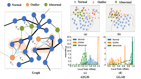
Figure 1. Left: An exemplar graph with the edge width indicates the level of affinity connecting two nodes, in which normal nodes (e.g., $v_{n_{i}}$ and $v_{n_{j}}$) have stronger affinity to its neighboring normal nodes than abnormal nodes (e.g., $v_{a_{i}}$ and $v_{a_{j}}$) due to homophily relation within the normal class. Our approach GGAD aims to generate outliers (e.g., $v_{o_{i}}$ and $v_{o_{j}}$) that share the same local neighborhood as the normal nodes (e.g., $v_{n_{i}}$ and $v_{n_{j}}$) but have significantly weaker affinity to these neighbors. Right: The outliers generated by methods like AEGIS (Ding et al., 2021) that ignore their structural relation often mismatch the distribution of abnormal nodes, as illustrated in (a), due to their false local affinity (see (c)). By contrast, GGAD incorporates the aforementioned homophily relation to generate outliers so that they well assimilate the local affinity of abnormal nodes (see (d)), and as a result, the outliers can well match the distribution of the abnormal nodes in the representation space, as illustrated in (b). Such outliers can help train a discriminative one-class classifier with a better decision boundary.

which are shown to be ineffective on non-Euclidean data like graph data (Ding et al., 2019; Zhuang et al., 2023; Qiao and Pang, 2023; Wang et al., 2023a; Liu et al., 2021b; Huang et al., 2022b). To address this challenge, as an emergent effective way of modeling graph data, graph neural networks (GNN) have been widely used for deep GAD (Ma et al., 2023). However, these methods typically assume that the labels of all nodes are unknown and perform anomaly detection in a fully unsupervised way by, e.g., data reconstruction (Ding et al., 2019; Fan et al., 2020), self-supervised methods (Liu et al., 2021b; Chen et al., 2020; Zhang et al., 2021; Meng et al., 2023), and recently one-class homophily modeling (Qiao and Pang, 2023). Although these methods achieve remarkable advances, they are not favored in many real applications where the labels for normal nodes are easy to obtain due to their overwhelming presence in a graph. This is because their capability to utilize those labeled normal nodes is largely limited due to their inherent unsupervised nature. There have been some GAD methods (Tang et al., 2022; Gao et al., 2023a; Huang et al., 2022a; Liu et al., 2021a; Tang et al., 2023; Wang et al., 2023c, b; Ma et al., 2023) designed in a semi-supervised setting that assumes the availability of both labeled normal and abnormal nodes during training. These methods often require a costly annotation of a large set of anomaly nodes since (i) anomalies are rare and unknown events and (ii) it is difficult, if not impossible, to have labeled anomalies to illustrate all possible types of anomaly. This greatly limits the practical application of these methods.

Different from the aforementioned two GAD settings, this paper instead considers a practical yet under-explored semi-supervised GAD scenario, where part of the nodes in the graph are known to be normal. Such a one-class classification setting has been widely explored in anomaly detection on other data types, such as visual data (Pang et al., 2021a; Cao et al., 2024), time series (Yang et al., 2023), and tabular data (Jiang et al., 2023), but it is rarely explored in anomaly detection on graph data. Recently there have been a few relevant studies in this line (Ma et al., 2022; Niu et al., 2023; Liu et al., 2023a; Cai et al., 2023; Xu et al., 2023), but they are on graph-level anomaly detection, i.e., detecting abnormal graphs from a set of graphs, while we explore the semi-supervised setting for abnormal node detection. We establish an evaluation benchmark for this problem and show that having access to these normal nodes helps enhance the detection performance of existing GAD methods, e.g., those unsupervised methods when they are properly adapted to the semi-supervised setting. However, due to their original unsupervised designs, they cannot make full use of these labeled normal nodes.

To better exploit those normal nodes, we propose a novel generative GAD approach, namely GGAD, aiming at generating outlier nodes that assimilate anomaly nodes in both local structure and node representations for providing effective negative node samples in training a discriminative one-class classifier on the given normal nodes. There have been many generative anomaly detection approaches that learn adversarial outliers to provide some weak supervision in training their detection models (Zheng et al., 2019; Sabokrou et al., 2021; Zenati et al., 2018; Ngo et al., 2019), but they are designed for non-graph data, and as a result, they fail to take account of the graph structure information. Some recent methods, such as AEGIS (Ding et al., 2021), attempt to adapt this approach for GAD, but the outliers are generated based on simply adding Gaussian noises to the GNN-based node representations, ignoring the structural relations between the outliers and the graph nodes. Consequently, the distribution of the generated outliers may lie at the fringe of the normal nodes, but it is often mismatched to that of the real anomaly nodes, as illustrated in Figure 1 (a).

Our approach, GGAD, tackles this issue with a graph structure-aware outlier generation method. It is motivated by an asymmetric local affinity phenomenon revealed in recent students (Qiao and Pang, 2023; Gao et al., 2023a, b), i.e., the affinity between normal nodes is typically significantly stronger than that between normal and abnormal nodes. More specifically, GGAD first generates outlier nodes based on the representations of the ego network (i.e., one-hop neighbors) of some randomly sampled normal nodes. GGAD then enforces a smaller local affinity of the outlier nodes to these local neighbors than the normal nodes, resulting in similar local structural affinity of the outlier nodes as the anomaly nodes in the representation space, as shown in Figure 1 (d). This helps guarantee good separability between the generated outliers and normal nodes. To avoid generating trivial outliers that distribute too far away from the normal nodes, we further introduce an egocentric closeness constraint to pull the outlier representations close to those sampled normal nodes. The resulting outliers can be well aligned to the distribution of the anomaly nodes, especially for those that have similar local affinity as the outlier nodes, while lying closely to the normal nodes, as shown in Figure 1 (b). We can then train a discriminative one-class classifier on the labeled normal nodes, with these generated outlier nodes treated as negative samples.

Our main contributions can be summarized as follows:

• We explore a practical yet under-explored semi-supervised GAD problem where part of the normal nodes are known, and establish an evaluation benchmark for the problem.

• We propose a novel generative GAD approach, GGAD, that aims to generate outlier nodes of similar local graph structure and node representations as the real anomaly nodes to provide effective negative samples for training a discriminative one-class classifier on the labeled normal nodes.

• We further introduce an innovative outlier node generation method, in which the generated outlier nodes are optimized to be separable from the normal nodes in their local affinity, while being enforced to achieve egocentric closeness to the normal nodes. The resulting outliers can well assimilate the abnormal nodes in both graph structure and node representation space. As far as we know, this is the first work for generating graph structure-aware outlier nodes for GAD.

• Extensive experiments on four large GAD datasets demonstrate that our approach GGAD substantially outperforms state-of-the-art unsupervised and semi-supervised GAD methods with varying numbers of training normal nodes.

2. Related Work

2.1. Graph Anomaly Detection

Numerous graph anomaly detection methods, including shallow and deep approaches, have been proposed. Shallow methods like Radar (Li et al., 2017), AMEN (Perozzi and Akoglu, 2016), and ANOMALOUS (Peng et al., 2018) are often bottlenecked due to the lack of representation power to capture the complex semantics of graphs. With the development of GNN in node representation learning, many deep GAD methods show better performance than shallow approaches. Here we focus on the discussion of the deep GAD methods in two settings: unsupervised and semi-supervised GAD.

Unsupervised Approach. Existing unsupervised GAD methods are typically built using a conventional anomaly detection objective, such as data reconstruction. The basic idea is to capture the normal activity patterns and detect anomalies that behave significantly differently. As one of the most popular methods, reconstruction-based methods using graph auto-encoder (GAE) have been widely applied for GAD (Bandyopadhyay et al., 2020). DOMINANT is the first work that applies GAE on the graph to reconstruct the attribute and structure leveraging GNNs (Ding et al., 2019). Fan et al. propose AnomalyDAE to further improve the performance by enhancing the importance of the reconstruction on the graph structure. In addition to reconstruction, some methods focus on exploring the relationship in the graph, e.g., the relation between nodes and subgraphs, to train GAD models. Among these methods, CoLA (Liu et al., 2021b) is one of the most popular methods, which attempts to learn the relations between the target nodes and their contextual subgraphs for GAD. SL-GAD (Zheng et al., 2021) is proposed to instead reconstruct the local subgraph. Huang et al. propose HCM-A (Huang et al., 2022b) to model both local and global contextual anomalies based on a hop count prediction objective. Qiao et al. propose TAM (Qiao and Pang, 2023), which maximizes the local node affinity on truncated graphs, achieving good performance on the synthetic dataset and datasets with real anomalies. Although the aforementioned unsupervised methods achieve good performance and help us identify anomalies without any access to class labels, they cannot effectively leverage the labeled nodes when such information is available.

Semi-Supervised Approach. The one-class classification under semi-supervised setting has been widely explored in anomaly detection on visual data, but rarely done on the graph data, except (Ma et al., 2022; Niu et al., 2023; Cai et al., 2023; Liu et al., 2023a; Xu et al., 2023) that recently explored this setting for graph-level anomaly detection. To detect abnormal graphs, these methods address a very different problem from ours, which is focused on capturing the normality of the given normal graphs in both the local and global structure scales. By contrast, we focus on modeling the normality at the node level. Some semi-supervised methods have been recently proposed for node-level anomaly detection, but they assume the availability of the labels of both normal and anomaly nodes (Park et al., 2022; Shi et al., 2022; Huang et al., 2022a; Liu et al., 2021a; Gao et al., 2023a; Liu et al., 2021a; Wang et al., 2023b).

Although these GAD methods achieve effective performance, they rely on the labeled anomaly data, which are often difficult to obtain.

2.2. Generative Anomaly Detection

Generative adversarial networks (GANs) provide an effective solution to generate synthetic samples that capture the normal/abnormal patterns (Goodfellow et al., 2020; Zhang et al., 2023). One type of these methods aims to learn latent features that can capture the normality of a generative network (Liu et al., 2023b; Zaheer et al., 2022). Methods like ALAD (Zenati et al., 2018), Fence GAN (Ngo et al., 2019) and OCAN (Zheng et al., 2019) are early methods in this line, aiming at making the generated samples lie at the boundary of normal data for more accurate anomaly detection. Motivated by these methods, a similar approach has also been explored in graph data, like AEGIS (Ding et al., 2021) and GAAN (Chen et al., 2020) which aim to simulate some abnormal features in the representation space using GNN, but they are focused on adding Gaussian noise to the representations of normal nodes without considering graph structure information. They are often able to generate pseudo anomaly node representations that are separable from the normal nodes for training their detection model, but the pseudo anomaly nodes are mismatched with the distribution of the real anomaly nodes.

3. Graph Structure-aware Outlier Node Generation

3.1. Problem Statements

Semi-supervised GAD. We focus on the semi-supervised anomaly detection on the attributed graph given some labeled normal nodes. An attributed graph is denoted by $\mathcal{G}=(\mathcal{V},\mathcal{E},\boldsymbol{X})$, where $\mathcal{V}=\left\{v_{1},\cdots,v_{N}\right\}$ denotes the node set, ${\mathcal{E}\subseteq\mathcal{V}\times\mathcal{V}}$ with $e\in\mathcal{E}$ is the edge set in the graph. ${e_{ij}=1}$ represents there is a connection between node $v_{i}$ and ${v_{j}}$, and ${e_{ij}=0}$ otherwise. The node attributes are denoted as $\bf{X}\in\mathbb{R}^{N\times F}$ and ${\bf{A}}\in\{0,1\}^{N\times N}$ is the adjacency matrix of $\mathcal{G}$. $\boldsymbol{x}_{i}\in\mathbb{R}^{F}$ is the attribute vector of $v_{i}$ and ${{\bf{A}}_{ij}=1}$ if and only if $\left(v_{i},v_{j}\right)\in\mathcal{E}$. ${{\mathcal{V}}_{n}}$ and ${\mathcal{V}}_{a}$ represent the normal node set and abnormal node set, respectively. Typically the number of normal nodes is significantly more than the anomalous nodes, i.e., $\left|{\mathcal{V}}_{n}\right|\gg\left|{\mathcal{V}}_{a}\right|$. The goal of semi-supervised GAD is to learn an anomaly scoring function $f:\mathcal{G}\rightarrow\mathbb{R}$, such that $f(v)<f(v^{\prime})$, $\forall v\in\mathcal{V}_{n},v^{\prime}\in\mathcal{V}_{a}$ given a set of labeled normal nodes $\mathcal{V}_{l}\subset{{\mathcal{V}}_{n}}$ and no access to labels of anomaly nodes. All other unlabeled nodes, denoted by $\mathcal{V}_{u}=\mathcal{V}\setminus\mathcal{V}_{l}$, comprise the test data set.

Outlier Node Generation. Outlier generation aims to generate outlier nodes that deviate from the normal nodes. Such nodes can be generated in either the raw feature space or the embedding feature space. This work is focused on the latter case, as it offers a more flexible way to represent relations between nodes. Our goal is to generate a set of outlier nodes from $\mathcal{G}$, denoted by ${\mathcal{V}}_{o}$, in the embedding space, so that the outlier nodes are separable from the labeled normal nodes ${\mathcal{V}}_{l}$, while lying at the fringe of the normal nodes to provide non-trivial supervision information of ground-truth abnormal nodes.

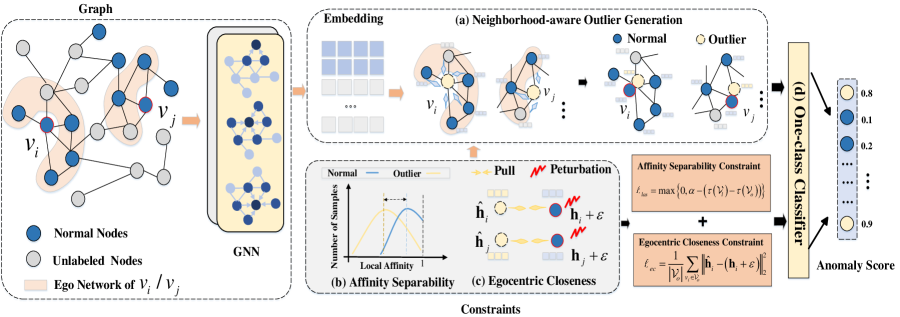
Figure 2. Overview of GGAD. (a) It first performs neighborhood-aware outlier node generation that produces the representation of outlier nodes based on the ego network of a normal node. We then introduce two constraints (b-c) to guarantee the quality of the generated outliers, including i) the local affinity separability constraint that enforces the separability between the normal and outlier nodes based on the affinity to their local neighbors, and ii) the egocentric closeness constraint that pulls the representations of the outlier nodes to the normal nodes that share the same ego network. (d) The resulting generated outlier nodes are lastly treated as negative samples to train a discriminative one-class classifier on the labeled normal nodes.

Graph Neural Network for Node Representation Learning GNN has been widely used to generate the node representation due to its powerful representation ability by capturing the rich graph attribute and structure information. The projection of node representation using GNN layer can be generally formalized as

(1) $${{\bf{H}}^{(\ell)}={\mathop{\rm GNN}\nolimits}\left({{{\bf{A}}},{\bf{H}}^{(\ell-1)};{{\bf{W}}^{(\ell)}}}\right),}$$

where ${\bf{H}}^{(\ell)}\in\mathbb{R}^{N\times h^{(l)}}$, ${\bf{H}}^{(\ell-1)}\in\mathbb{R}^{N\times h^{(l-1)}}$ are the representations of all $N$ nodes in the ${(\ell)}$-th layer and ${(\ell-1)}$-th layer, respectively, $h^{(l)}$ is the dimensionality size, ${\bf{W}}^{(\ell)}$ are the learnable parameters, and ${\bf{H}}^{(0)}$ is set to $\mathbf{X}$. ${{{\bf{H}}^{(\ell)}}=\left\{{{{\bf{h}}_{1}},{{\bf{h}}_{2}},\ldots,{{\bf{h}}_{N}}}\right\}}$ is a set of representations of $N$ nodes in the last GNN layer, with ${{{\bf{h}\in{\mathbb{R}}}^{d}}}$. In this paper, we adopt a 2-layer GCN to model the graph.

3.2. Learning Outlier Node Representations from Ego Networks of Normal Nodes

The key intuition behind GGAD is to generate outlier nodes that assimilate anomaly nodes in terms of both local graph structure and node representations. To this end, we first introduce a neighborhood-aware outlier generation module that generates the outlier nodes’ representation based on the representations of the local neighbors of normal nodes. The representations from these neighbor nodes provide an important reference for being normal in a local graph structure, upon which we learn the outlier node representations that deviate from this referenced representation. This helps ground the generation of outlier nodes to a real graph structure.

More specifically, as shown in Fig. 2(a), given a labeled normal node $v_{i}\in\mathcal{V}_{l}$ and its ego network $\mathcal{N}(v_{i})$ that contains all nodes directly connected with $v_{i}$, we generate an outlier node in the representation space by:

(2) $${{\hat{\bf{h}}_{i}}=\Psi\left(v_{i},{{\mathcal{N}}({v_{i}});\Theta_{g}}\right)=\frac{1}{|{\mathcal{N}}(v_{i})|}\sum\limits_{{v_{j}}\in{\mathcal{N}}({v_{i}})}\sigma({{\bf{\tilde{W}}}}{{\bf{h}}_{j}})},$$

where $\Psi$ is a mapping function determined by parameters $\Theta_{g}$ that contain the learnable parameters ${\bf{\tilde{W}\in{\mathbb{R}}}}^{d\times d}$ in this module in addition to the parameters ${\bf{W}}^{(\ell)}$ in Eq. (1), and ${\sigma(\cdot)}$ is an activation function. It is not required to perform Eq. (2) for all training normal nodes. We sample a set of $S$ normal nodes from $\mathcal{V}_{l}$ and respectively generate an outlier node for each of them based on its ego network.

${\hat{\bf{h}}_{i}}$ in Eq. (2) serves as an initial representation of the outlier node. In the next two subsections, we introduce two optimization constraints to enable the learning of outlier nodes that assimilate real abnormal nodes in graph structure and node representation.

3.3. Enforcing Local Affinity Separability Between Outlier Nodes and Normal Nodes

To incorporate graph structure information into outlier node generation, we leverage one crucial asymmetric homophily phenomenon in which normal nodes tend to have a strong connection/affinity with each other, while the affinity of abnormal nodes is significantly weaker than normal nodes.

To this end, GGAD introduces a local affinity separability constraint to enforce that the local affinity of the generated outlier nodes to their local neighbors should be smaller than that of the normal nodes, as illustrated in Fig. 2(b).

More specifically, the local node affinity of $v_{i}$, denoted as $\tau(v_{i})$, is defined as the similarity to its neighboring nodes:

(3) $${\tau\left({{v_{i}}}\right)=\frac{1}{{\left|{{\mathcal{N}}\left({{v_{i}}}\right)}\right|}}\sum\limits_{{v_{j}}\in{\mathcal{N}}\left({{v_{i}}}\right)}{{\mathop{\rm sim}\nolimits}}\left({{{\bf{h}}_{i}},{{\bf{h}}_{j}}}\right)},$$

The local affinity separability is then defined by a margin loss function based on the affinity of the normal nodes and the generated outlier nodes as follows:

(4) $${\ell_{las}}=\max\left\{{0,\alpha-\left({\tau\left({{\mathcal{V}}_{l}}\right)-\tau\left({\mathcal{V}}_{o}\right)}\right)}\right\},$$

where $\tau\left({{\mathcal{V}}_{o}}\right)=\frac{1}{{\left|{{\mathcal{V}}_{o}}\right|}}\sum\limits_{{v_{i}}\in{{\mathcal{V}}_{o}}}\tau\left({{v_{i}}}\right)$ and $\tau\left({{\mathcal{V}}_{l}}\right)=\frac{1}{{\left|{{{\mathcal{V}}_{l}}}\right|}}\sum\limits_{{v_{i}}\in{{\mathcal{V}}_{l}}}\tau\left({{v_{i}}}\right)$ represent the average local affinity of the normal and outlier nodes respectively, and $\alpha>0$ is a hyperparameter controlling the margin between the affinities of these two types of nodes. Eq. (4) enforces this separability at the node set level rather than at each individual outlier node, as the latter case would be highly computationally costly when $\mathcal{V}_{l}$ or $\mathcal{V}_{o}$ is large.

It should be noted that solely adding this affinity separability constraint may generate trivial outliers that distribute far away from the normal nodes in the representation space, as shown in Figure 3(a). For those trivial outliers, although they achieve similar local affinity to the abnormal nodes, as shown in Figure 3(d), they are still not aligned well with the distribution of the abnormal nodes, and thus, they cannot serve as effective negative samples for learning the one-class classifier on the normal nodes. Thus, we further introduce an egocentric closeness constraint in the next subsection to address this issue.

3.4. Regularizing Outlier Node Representations with Egocentric Closeness

Due to the over-smoothing representation issue in GNNs, the representations of the abnormal and normal nodes often do not have large differences. Thus, if the generated outlier nodes lie far away from the normal nodes, they fail to assimilate the abnormal nodes in the node representation space. To tackle this issue, as illustrated in Fig. 2(c), we further introduce an egocentric closeness constraint to pull the representations of the outlier nodes closed to the normal nodes that share the same ego network as the outlier nodes. More specifically, let ${{\bf{h}}_{i}}$ and ${{{\hat{\bf{h}}}_{i}}}$ be the representations of the normal node $v_{i}$ and its corresponding generated outlier node that shares the same ego network as $v_{i}$ (as discussed in Sec. 3.2), the egocentric closeness constraint ${{\ell_{{ec}}}}$ is defined as follows:

(5) $${\ell_{ec}}=\frac{1}{{\left|{{{\mathcal{V}}_{o}}}\right|}}\sum\limits_{{v_{i}}\in{{\mathcal{V}}_{o}}}{\left\|{{{\hat{\bf{h}}}_{i}}-\left({{{\bf{h}}_{i}}+\varepsilon}\right)}\right\|_{2}^{2}},$$

where ${\left|{{{\mathcal{V}}_{o}}}\right|}$ is the number of the generated outliers and $\epsilon$ is a noise perturbation generated from a Gaussian distribution. The perturbation is added to guarantee a separability between ${{\bf{h}}_{i}}$ and ${{{\hat{\bf{h}}}_{i}}}$, while enforcing its egocentric closeness.

As shown in Fig. 3(c), using this egocentric closeness constraint together with the affinity separability helps effectively tie the representations of the outlier nodes to the normal nodes but they are very separable from each other. Thus, using both constraints/terms results in well-aligned distributions between the generated outliers and the real abnormal nodes in both the representation space and the local structure, as illustrated in Figs. 3(c) and (f), respectively. Using the egocentric closeness alone also results in mismatches between the generated outlier nodes and the abnormal nodes (see Fig. 3(e)) since it ignores the local structure relation of the generated outlier nodes.

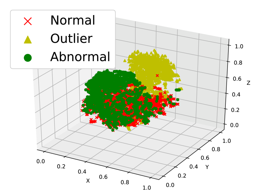
(a) t-SNE of Using ${\ell_{las}}$ Only

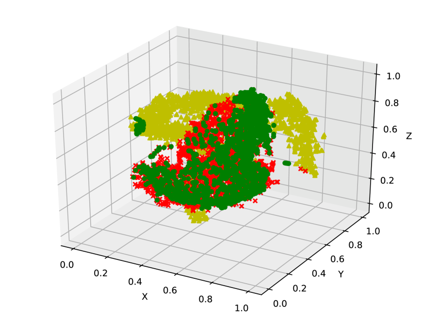
(b) t-SNE of Using ${\ell_{ec}}$ only

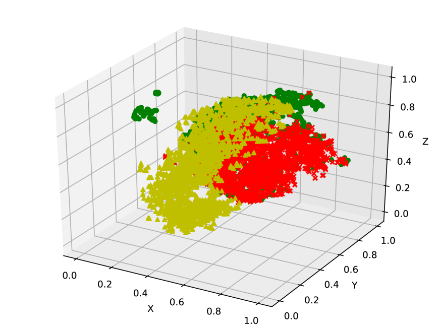
(c) t-SNE of Using GGAD

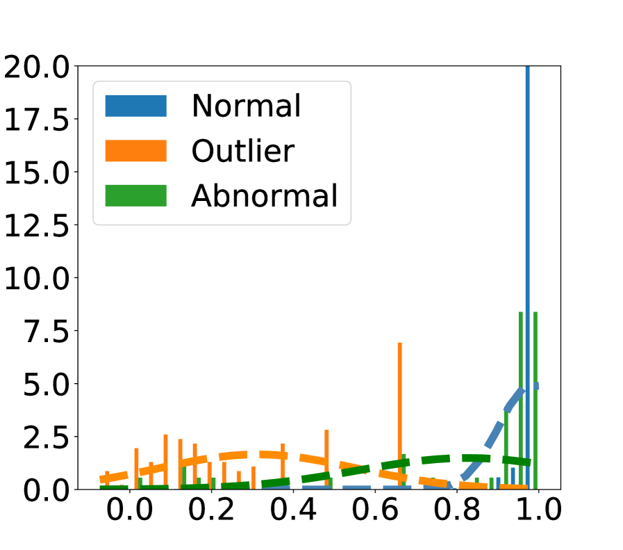
(d) Using ${\ell_{las}}$ Only

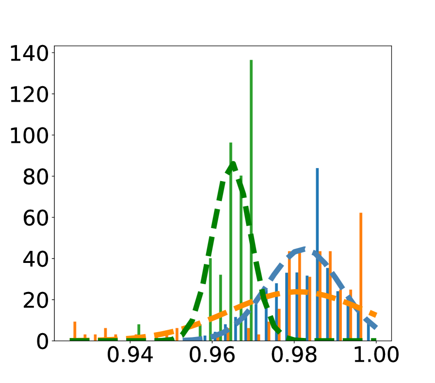
(e) Using ${\ell_{ec}}$ Only

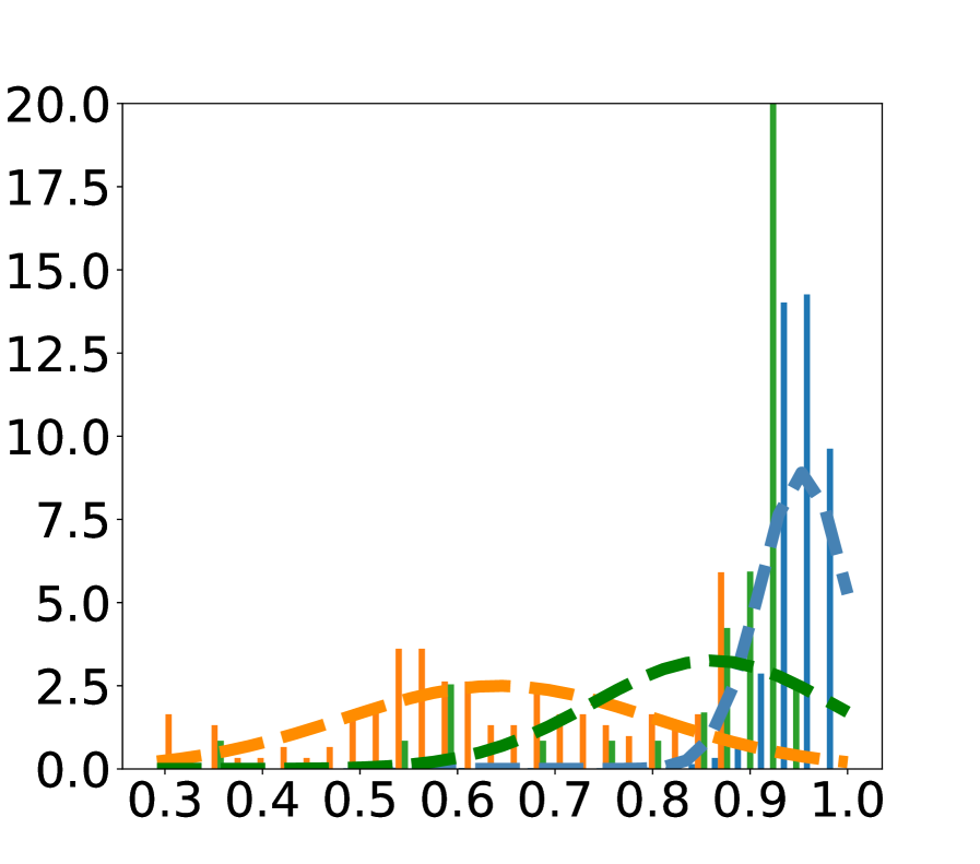
(f) Using GGAD

Figure 3. t-SNE visualization of the node representations and histograms of local affinity yielded by GGAD and its two variants on a fraud detection dataset T-Finance (Tang et al., 2022).

3.5. One-class Classification with the Generated Outlier Nodes

Training. Since the generated outlier nodes are to assimilate the abnormal nodes, they can be used as important negative samples to train a one-class classifier on on the labeled normal nodes. We implement this classifier using a fully connected layer on top of the GCN layers that maps the node representations to a prediction probability-based anomaly score, denoted by $\eta:\mathbf{H}\rightarrow\mathbb{R}$, followed by a binary cross-entropy (BCE) loss function $\ell_{bce}$:

(6) $${\ell_{bce}=\sum\limits_{i}^{N}{{y_{i}}\log({p_{i}})+(1-{y_{i}})}\log(1-{p_{i}})},$$

where $p_{i}=\eta(\mathbf{h}_{i};\Theta_{s})$ is the output of the one-class classifier indicating the probability that a node is a normal node, and $y$ is the label of node. We set $y=1$ if the node is a labeled normal node, and $y=0$ if the node is a generated outlier node. The one-class classifier is jointly optimized with the affinity separable constraint ${\ell_{{las}}}$ and egocentric closeness constraint ${\ell_{{ec}}}$ in an end-to-end manner. Thus, the overall loss ${\ell_{{total}}}$ is formalized as:

(7) $${\ell_{{total}}}={\ell_{bce}}+\beta{\ell_{{las}}}+\lambda{\ell_{{ec}}},$$

where $\beta$ and $\lambda$ are the hyperparameters to control the importance of the two constraints respectively. The learnable parameters are $\Theta=\{\Theta_{g},\Theta_{s}\}$.

Inference. During inference, we can directly use the inverse of the prediction of the one-class classifier as the anomaly score:

(8) $${\mathop{\rm score}\nolimits}\left({{{v}_{j}}}\right)=1-\eta\left(\mathbf{h}_{j};\Theta^{*}\right),$$

where $\Theta^{*}$ is the learned parameters of GGAD. Since our outlier nodes well assimilate the real abnormal nodes, they are expected to receive high anomaly scores from the one-class classifier.

Table 1. Key statistics of the datasets used in our experiments.

Data set	Type	Nodes	Edges	Attributes	Anomalies(Rate)
Amazon	Co-review	11,944	175,608	25	796(6.66%)
T-Finance	Transaction	39,357	21,222,543	10	1,803(4.6%)
Reddit	Social Media	10,984	175,608	64	366(3.33%)
DGraph	Social Networks	3,700,550	73,105,508	17	15,509(1.3%)

4. Experiments

4.1. Datasets

We conduct experiments on four large real-world graph datasets with genuine anomalies from diverse domains, including the co-review network in Amazon (Dou et al., 2020), transaction record network in T-Finance (Tang et al., 2022), and social networks in Reddit (Kumar et al., 2019) and DGraph (Huang et al., 2022c). Their key statistics are presented in Table LABEL:tab:datasets. More specifically, Amazon is a graph capturing the relations between users and products, in which we aim to identify malicious users who are paid to write fake reviews for products. T-Finance is a transaction network where edges represent the transaction records between users. The anomalies such as fraud, money laundering, and online gambling are labeled by human experts. Reddit is a network of forum posts from Reddit in which the users who have been blocked from the platform are regarded as anomalies. DGraph is a large-scale social network provided by Finvolution Group, in which each node represents a user, an edge indicates the emergency contact information among users, and anomalies are users who have suspicious fraudulent behaviors. See App. A for more details about the datasets.

Although it is easy to obtain normal nodes, the human checking and annotation of large-scale nodes are still costly. To simulate practical scenarios where we need to annotate only a relatively small number of normal nodes, we randomly sample $R$% of the normal nodes as labeled normal data for training, in which $R$ is chosen in $\{10,15,20,25\}$, with the rest of nodes is treated as the testing set. The same $R$ applied to DGraph would lead to a significantly larger set of normal nodes than the other three data sets, leading to very different annotation costs in practice. Thus, on DGraph, $R$ is chosen in $\{0.05,0.2,0.35,0.5\}$ to compose the training data.

Table 2. AUROC and AUPRC results on four real-world GAD datasets. The best performance per dataset is boldfaced, with the second-best underlined. ‘/’ indicates that the model cannot handle the huge size of nodes in DGraph.

Setting	Method	Dataset
		AUROC				AUPRC
		Amazon	T-Finance	Reddit	DGraph	Amazon	T-Finance	Reddit	DGraph
Unsupervised	DOMINANT	0.7025	0.6087	0.5105	0.5738	0.1315	0.0536	0.0380	0.0075
	AnomalyDAE	0.7783	0.5809	0.5091	0.5763	0.1429	0.0491	0.0319	0.0070
	OCGNN	0.7165	0.4732	0.5246	/	0.1352	0.0392	0.0375	/
	AEGIS	0.6059	0.6496	0.5349	0.4509	0.1200	0.0622	0.0413	0.0053
	GAAN	0.6513	0.3091	0.5216	/	0.0852	0.0283	0.0348	/
	TAM	0.8303	0.6175	0.6062	/	0.4024	0.0547	0.0437	/
Semi-supervised	DOMINANT	0.8867	0.6167	0.5194	0.5851	0.7289	0.0542	0.0414	0.0076
	AnomalyDAE	0.9171	0.6027	0.5280	0.5866	0.7748	0.0538	0.0362	0.0071
	OCGNN	0.8810	0.5742	0.5622	/	0.7538	0.0492	0.0400	/
	AEGIS	0.7593	0.6728	0.5605	0.4450	0.2616	0.0685	0.0441	0.0058
	GAAN	0.6531	0.3636	0.5349	/	0.0856	0.0324	0.0362	/
	TAM	0.8405	0.5923	0.5829	/	0.5183	0.0551	0.0446	/
	GGAD (Ours)	0.9443	0.8228	0.6354	0.5943	0.7922	0.1825	0.0610	0.0082

4.2. Competing Methods and Evaluation Metric

Competing Methods. To our best knowledge, there exist no GAD methods specifically designed for semi-supervised anomalous node detection. To validate the effectiveness of GGAD, we compare it with six state-of-the-art (SOTA) unsupervised methods and their advanced versions in which we effectively adapt them to our semi-supervised setting. These methods include two reconstruction-based models: DOMINANT (Ding et al., 2019) and AnomalyDAE(Fan et al., 2020), two one-class classification models: TAM (Qiao and Pang, 2023) and OCGNN (Wang et al., 2021), and two generative models: AEGIS (Ding et al., 2021) and GAAN (Chen et al., 2020).

To effectively incorporate the normal information into these unsupervised methods, for the reconstruction models, DOMINANT and AnomalyDAE, the data reconstruction is performed on the labeled normal nodes only during training. In OCGNN, the one-class center is optimized based on the labeled normal nodes exclusively. In TAM, we train the model by maximizing the affinity on the normal nodes only. As for AEGIS and GAAN, the normal nodes combined with their generated outliers are used to train the adversarial network. Self-supervised-based methods like CoLA (Liu et al., 2021b), SL-GAD(Chen et al., 2020), and HCM-A (Huang et al., 2022b) are omitted in our comparison because training these methods on the data with exclusively normal nodes does not work.

Evaluation Metric. Following prior studies (Chai et al., 2022; Pang et al., 2021b; Wang et al., 2023a), two popular and complementary evaluation metrics for anomaly detection, the area under ROC curve (AUROC) and Area Under the precision recall curve (AUPRC), are used to evaluate the performance. Higher AUROC/AUPRC indicates better performance. AUROC reflects the ability to recognize anomalies while at the same time considering the false positive rate. AUPRC focuses solely on the precision and recall rates of detecting anomalies. The AUROC and AUPRC results are averaged over 5 runs with different random seeds.

4.3. Implementation Details

GGAD is implemented in Pytorch 1.6.0 with Python 3.7. and all the experiments are run on a 24-core CPU. In GGAD, its weight parameters are optimized using Adam (Kinga et al., 2015) optimizer with a learning rate of $1e-3$ by default. For each dataset, the hyperparameters $\beta$ and $\lambda$ for two constraints are uniformly set to 1, though GGAD can perform stably with a range of $\beta$ and $\lambda$ (see Sec. 4.7). The size of the generated outlier nodes $S$ is set to 5% of $|\mathcal{V}_{l}|$ by default and stated otherwise. The affinity margin $\alpha$ is set to 0.7 across all datasets. The perturbation in Eq. (5) is drawn from a Gaussian perturbation. All the competing methods are implemented by using their publicly available official source code or the library, and they are trained using suggested hyperparameters. To apply GGAD and the competing models to very large graph datasets, i.e., DGraph, a min-batch training strategy is applied (see Algorithm 1 for detail).

4.4. Main Comparison Results

Table 2 shows the comparison of GGAD to 12 models, in which semi-supervised models use 15% normal nodes during training while unsupervised methods are trained on the full graph in a fully unsupervised way. We will discuss results using more/less training normal nodes in Sec. 4.5.

Comparison to Unsupervised GAD Methods. As shown in Table 2, GGAD significantly outperforms all unsupervised methods on four datasets, having maximally 21% AUROC and 39% AUPRC improvement over the best-competing unsupervised methods on individual datasets. The results also show that the semi-supervised versions of the unsupervised methods largely improve the performance of their unsupervised counterparts, justifying that i) incorporating the normal information into the unsupervised approaches is beneficial for enhancing the detection performance and ii) our approach to adapt the unsupervised methods is effective across various types of GAD models. TAM performs best among the unsupervised methods. AEGIS which leverages GAN to learn the normal patterns performs better than AnomalyDAE and DOMINANT on the T-Finance and Reddit, By contrast, reconstruction-based approaches work well on Amazon and DGraph. Similar observations can be found for the semi-supervised versions.

Comparison to Semi-supervised GAD Methods. The results show that although the semi-supervised methods largely outperform their unsupervised counterparts, they substantially underperform our method GGAD. The reconstruction-based approaches show the most competitive performance among the contenders in semi-supervised setting, e.g., AnomalyDAE performs best on Amazon and DGraph. Nevertheless, GGAD gains respectively about 1-3% AUROC/AUPRC improvement on these two datasets compared to the best competing model AnomalyDAE. Methods like TAM and AEGIS, which benefit from the representation ability of GNN in the embedding space and training on the normal nodes under the semi-supervised setting, largely reduce the interference of abnormal nodes on the model and work well on most of the datasets, e.g., TAM on Amazon and Reddit, AEGIS on T-Finance and Reddit. However, their performance is still lower than GGAD by a relatively large margin. These results demonstrate that, benefiting from our outlier node generation and the discriminative one-class classifier, our method GGAD can leverage the labeled normal nodes substantially more effectively than all competing methods.

4.5. Performance with Varying Normal Nodes

In order to further illustrate the effectiveness of our method, we also compare the performance of GGAD with other semi-supervised methods with varying numbers of normal nodes available during training. The AUPRC results on the four datasets are shown in Fig. 4. The results show that with increasing training samples of normal nodes, the performance of all methods on all four datasets generally gets improved since more normal samples can help the models more accurately capture the normal patterns during training. Importantly, GGAD consistently outperforms all competing methods with varying numbers of normal nodes, reinforcing our observation that GGAD can make better use of the labeled normal nodes for GAD. A similar observation can be found in AUROC in App. C.1.

4.6. Ablation Study

Effects of the Two Constraints. The importance of our proposed optimization constraints is examined by comparing our full model with its variant removing the corresponding constraint, with the results shown in Table 3. It is clear that learning the outlier node representations using one constraint solely with the $\ell_{bce}$ loss performs remarkably less effectively than our full model using both constraints. It is mainly because although using $\ell_{las}$ solely can obtain similar local affinity of the outliers as the abnormal nodes, the outliers are still not aligned well with the distribution of the abnormal nodes in the node representation space. Likewise, only using the $\ell_{ec}$ constraint can result in a mismatch between the generated outliers and real abnormal samples in their local graph structure perspective. GGAD that effectively unifies both constraints can generate outlier nodes that well assimilate the real abnormal nodes on both local structure and the node representation space, supporting substantially more accurate GAD performance.

Table 3. Ablation study results for our proposed constraints.

Metric	Component		Dataset
	${\ell_{{las}}}$	${\ell_{{lec}}}$	Amazon	T-Finance	Reddit	DGraph
AUROC		✓	0.8871	0.8149	0.5839	0.5891
	✓		0.7250	0.6994	0.5230	0.5513
	✓	✓	0.9324	0.8228	0.6354	0.5943
AUPRC		✓	0.6643	0.1739	0.0409	0.0076
	✓		0.1783	0.0800	0.0398	0.0063
	✓	✓	0.7843	0.1924	0.0610	0.0087

Our Graph Structure-aware Outlier Generation vs. Alternative Approaches To examine its effectiveness further, GGAD is compared with four other approaches that could be used as an alternative to generate the outliers. These include (i) Random that randomly sample some normal nodes and treat them as outliers to train a one-class discriminative classifier, (ii) Non-learnable Outliers (NLO) that removes the learnable parameters ${\bf{\tilde{W}}}$ in Eq. (2) in our neighbor-aware outlier generation, (iii) Noise that directly generates the representation of outlier nodes from random noise, and (iv) Gaussian Perturbation (GaussianP) that directly adds Gaussian perturbations into the sampled normal nodes’ representations as the outliers. The empirical results are shown in Table 4. Random does not work properly, since the randomly selected samples are not distinguishable from the normal nodes. NLO

Table 4. GGAD vs. alternative outlier generators.

Metric	Method	Dataset
		Amazon	T-Finance	Reddit	DGraph
AUROC	Random	0.7263	0.4613	0.5227	0.5712
	NLO	0.8613	0.6179	0.5638	0.5538
	Noise	0.8508	0.8204	0.5285	0.5779
	GaussianP	0.2279	0.6659	0.5235	0.5862
	GGAD (Ours)	0.9324	0.8228	0.6354	0.5943
AUPRC	Random	0.1755	0.0402	0.0394	0.0061
	NLO	0.4696	0.1364	0.0495	0.0065
	Noise	0.5384	0.1762	0.0381	0.0076
	GaussianP	0.0397	0.0677	0.0376	0.0078
	GGAD (Ours)	0.7843	0.1924	0.0610	0.0087

performs fairly well on some data sets such as Amazon and T-Finance, but it is still much lower than GGAD, showcasing that having learnable outlier node representations can help better ground the outliers in a real local graph structure.

Despite that Noise and GaussianP can generate outlier nodes that have separable node representations from the normal nodes, they also fail to work well since the lack of constraints on the local structure/affinity of the outlier nodes can lead to mismatched distributions between the generated outlier nodes and the abnormal nodes.

4.7. Sensitivity and Robustness Analysis

This section analyzes the sensitivity of GGAD w.r.t four key hyperparameters. The AUPRC results are reported in Fig. 5 (see App. C.2 for the AUROC results). We discuss these results below.

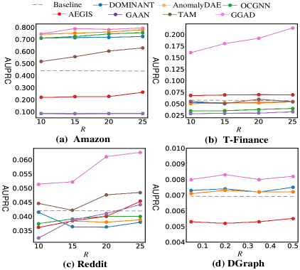
Figure 4. AUPRC results w.r.t different number of training normal nodes ($R$% of $|\mathcal{V}|$). DGraph is a very large dataset, so a significantly smaller $R$ is used to have a similar size of $\mathcal{V}_{l}$ as the other three datasets. ‘Baseline’ denotes the performance of the best unsupervised GAD method per dataset.

Impact of Margin $\alpha$ in $\ell_{las}$. $\alpha$ in $\ell_{las}$ denotes the affinity difference we enforce between the normal and outlier nodes. As Fig. 5 (a) shows, GGAD performs best on Amazon with increasing $\alpha$ while it performs stably on the other three datasets with varying $\alpha$, indicating that enforcing local separability is more effective on Amazon than the other datasets, as can also be observed in Table 4.

Impact of Hyperparameters $\beta$ and $\lambda$. As shown in Figs. 5 (b) and (c), with increasing $\beta$ and $\lambda$, our model GGAD generally performs better, indicating that a stronger affinity separability or egocentric closeness constraint is generally preferred to generate outlier nodes that are more aligned with the real abnormal nodes.

The Number of Generated Outlier Nodes $S$. As shown in Fig. 5 (d), where $S$ indicates that we generate the outlier nodes in a quantity at a rate of $S$% of $|\mathcal{V}_{l}|$, GGAD gains some improvement with more generated outlier nodes but it maintains the same performance after a certain number of outlier nodes. This is mainly because the generated outlier nodes may not be diversified enough to resemble all types of abnormal nodes, even with more outlier nodes. The decline performance on Amazon is mainly due to the fact that the labeled normal data there is small and is overwhelmed by increasing outliers nodes, leading to a worse training of the one-class classifier.

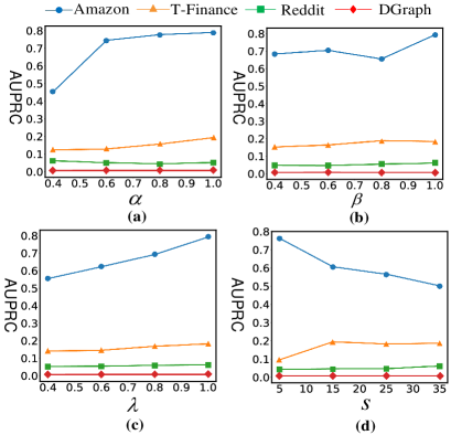
Figure 5. AUPRC of GGAD w.r.t hyperparameters $\alpha$, $\beta$, $\lambda$, $S$.

Robustness w.r.t. Anomaly Contamination. The labeled normal nodes can often be contaminated by anomalies due to factors like annotation errors. To consider this issue, we introduce a certain ratio of anomaly contamination into the labeled normal node for training, including 5%, 10%, 15%, or 20% of the total abnormal nodes into the training normal node set $\mathcal{V}_{l}$. The AUPRC results of the semi-supervised models under different ratios of contamination are shown in Fig. 6.

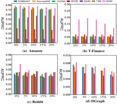
Figure 6. AUPRC w.r.t. different anomaly contamination.

It can be seen that with increasing anomaly contamination, the performance of all methods decreases. The reconstruction-based methods DOMINANT and AnomalyDAE are the most sensitive models, followed by GAAN, TAM, and AEGIS. OCGNN is relatively stable under the contamination. Despite the decreased performance, our method GGAD still maintains the best performance under different contamination rates.

4.8. Computational Efficiency

The runtimes, including both training and inference time, of GGAD and six semi-supervised competing methods on CPU are shown in Table 5.

In GGAD, although calculating the local affinity of each node requires some overheads, it is still much more efficient than the reconstruction operations on both the attributes and the structure as in DOMINANT and AnomalyDAE. Compared to the generative models AEGIS and GAAN, GGAD is generally more efficient on larger graph datasets like Amazon, T-Finance, and DGraph. OCGNN is a model with the simplest operation, to which our GGAD can also have comparable efficiency. These results demonstrate the advantage of GGAD in computational efficiency (see App. D for detailed complexity analysis of GGAD).

Table 5. Runtimes (in seconds) on the four datasets on CPU.

Method	Dataset
	Amazon	T-Finance	Reddit	DGraph
DOMINANT	1592	10721	125	388
AnomalyDAE	1656	18560	161	457
OCGNN	765	5717	162	/
AEGIS	1121	15258	166	1022
GAAN	1678	12120	94	/
TAM	4516	17360	432	/
GGAD (Ours)	658	9345	368	488

5. Conclusion

In this paper, we investigate a new semi-supervised GAD scenario where part of normal nodes are known during training. To fully exploit those normal nodes, we introduce a novel outlier generation approach GGAD that leverages the asymmetric affinity separability from the normal nodes and the egocentric closeness to the normal nodes to generate outlier nodes that well assimilate real abnormal nodes in both local graph structure and representation space. The quality of these outlier nodes is justified by their use in training a discriminative one-class classifier together with the given normal nodes. Comprehensive experiments are performed to establish an evaluation benchmark on four real-world datasets for semi-supervised GAD, in which our GGAD shows superior detection performance over 12 competing methods across the four datasets.

Appendix A Detailed Dataset Description

A detailed introduction of the four datasets we use is given as follows.

• Amazon (Dou et al., 2020): It includes product reviews under the Musical Instrument category. The users with more than 80% of helpful votes were labeled as begin entities, with the users with less than 20% of helpful votes treated as fraudulent entities. There are three relations including U-P-U (users reviewing at least one same product), U-S-U (users giving at least one same star rating within one week), and U-V-U (users with top-5% mutual review similarities). In this article, we do not distinguish this connection and regard them as the same type of edges, i.e., all connections are used. There are 25 handcrafted features that were collected as the raw node features.

• T-Finance (Tang et al., 2022): It is a financial transaction network where the node represents an anonymous account and the edge represents two accounts that have transaction records. The features of each account are related to some attributes of logging like registration days, logging activities, and interaction frequency, etc. The users are labeled as anomalies when they fall into the categories like fraud money laundering and online gambling.

• Reddit (Kumar et al., 2019): It is a user-subreddit graph, capturing one month’s worth of posts shared across various subreddits at Reddit. The users who have been banned by the platform are labeled anomalies. The text of each post is transformed into the feature vector and the features of the user and subreddits are the feature summation of the post they have posted.

• DGraph (Huang et al., 2022c): It is a large-scale attributed graph with millions of nodes and edges where the node represents a user account in a financial company and the edge represents that the user was added to another account as an emergency contact. The feature of a node is the profile information of users, such as age, gender, and other demographic features. The users who have overdue history are labeled as anomalies.

Appendix B Description of algorithms

B.1. Competing Methods

A more detailed introduction of the six GAD models we compare with is given as follows.

• DOMINANT (Ding et al., 2019) leverages the auto-encoder for graph anomaly detection. It consists of an encoder layer and a decoder layer which are devised to reconstruct the features and structure of the graph. The reconstruction errors from the features and the structural modules are combined as an anomaly score.

• AnomalyDAE (Fan et al., 2020) consists of a structure autoencoder and an attribute autoencoder to learn both node embeddings and attribute embeddings jointly in a latent space. In addition, an attention mechanism is employed in the structure encoder to capture normal structural patterns more effectively.

• OCGNN (Wang et al., 2021) applies one-class SVM and GNNs, aiming at combining the recognition ability of one-class classifiers and the powerful representation of GNNs. A one-class hypersphere learning objective is used to drive the training of the GNN. The sample that falls outside the hypersphere is defined as an anomaly.

• AEGIS (Ding et al., 2021) designs a new graph neural layer to learn anomaly-aware node representations and further employ generative adversarial networks to detect anomalies among new data. The generator takes noises sampled from a prior distribution as input, and attempts to generate informative potential anomalies. The discriminator tries to distinguish whether an input is the representation of a normal node or a generated anomaly.

• GAAN (Chen et al., 2020) is based on a generative adversarial network where fake graph nodes are generated by a generator. To encode the nodes, they compute the sample covariance matrix for real nodes and fake nodes, and a discriminator is trained to recognize whether two connected nodes are from a real or fake node.

• TAM (Qiao and Pang, 2023) learns tailored node representations for a new anomaly measure by maximizing the local affinity of nodes to their neighbors. TAM is optimized on truncated graphs where non-homophily edges are removed iteratively. The learned representations result in significantly stronger local affinity for normal nodes than abnormal nodes. So, a local affinity-based anomaly measure is used to calculate the anomaly score.

B.2. Publicly Available Official Source Code.

All the competing methods except TAM are implemented by PyGOD Library (Liu et al., 2022a, b). The code of TAM is taken from its authors. The links to their source codes are as follows:

• PyGOD: https://github.com/pygod-team/pygod

• TAM: https://github.com/mala-lab/TAM-master

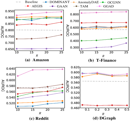
Figure 7. AUROC results w.r.t different number of training normal nodes ($R$% of $|\mathcal{V}|$). DGraph is a very large dataset, so a significantly smaller $R$ is used to have a similar size of $\mathcal{V}_{l}$ as the other three datasets. ‘Baseline’ denotes the performance of the best unsupervised GAD method per dataset.

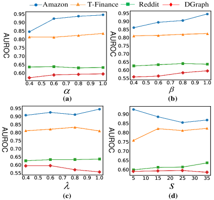
Figure 8. AUROC results w.r.t hyperparameters $\alpha$, $\beta$, $\lambda$, $S$.

Algorithm 1 Mini-Batch Processing

Input: Graph, ${{\mathcal{G}}{\rm{=}}\left({{\mathcal{V}},{\mathcal{E}},{\bf{X}}}\right)}$, ${N}$: Number of nodes, $t$: Batch size, ${z}$: Number of batches, ${S}$: The number of the generated outlier nodes, $\mathcal{V}_{train}$:Training set

Output: Mini-batches and sub-graph structure.

1:  Initialize the batch $\bf{B}={(\mathbf{b}_{1},...,\mathbf{b}_{z})}$, where $\mathbf{b}=[v_{1},...,v_{t}]$ from given $\mathcal{V}_{train}$

2:  for  each $\mathbf{b}$ in $\bf{B}$  do

3:     Sample $S/z$ nodes as initial outliers ${[v_{{o}_{1}},...v_{{o}_{S}}]}$ from batch $\mathbf{b}$

4:     Initialize a node set $\mathcal{V}_{\mathbf{b}}$ for batch $\mathbf{b}$

5:     for  each $v$ in $\mathbf{b}$ do

6:        Find the 2-hop neighborhoods $\mathcal{N}^{2}_{v}$ of $v$ and add them in node set $\mathcal{V}_{\mathbf{b}}$

7:     end for

8:     Build a sub-graph structure ${\mathcal{E}}_{\mathbf{b}}$ for batch $\bf{b}$ using node set $\mathcal{V}_{\mathbf{b}}$

9:  end for

10:  return  The batch ${\bf{B}}={({\mathbf{b}_{1}},...,\mathbf{b}_{z})}$ and sub-graph structure ${[\mathcal{E}_{1},...,\mathcal{E}_{z}]}$

Algorithm 2 GGAD

Input: Graph, ${{\mathcal{G}}{\rm{=}}\left({{\mathcal{V}},{\mathcal{E}},{\bf{X}}}\right)}$, ${N}$: Number of training nodes, , ${N_{u}}$: Number of unlabeled nodes, ${L}$: Number of layers, ${E}$: Training epochs, $\mathcal{V}_{train}$:Training set, $\mathcal{V}_{test}$:Test set , $S$: The number of the generated outlier nodes

Output: Anomaly scores of all nodes.

1:  Sample the ego networks of some normal nodes for outlier nodes to be generated ${\mathcal{V}_{o}=[v_{o_{1}},...,v_{o_{s}}]}$

2:  Then $\mathcal{V}_{train}$ consists of the outlier nodes ${\mathcal{V}_{o}}$ and the given labeled normal node set ${\mathcal{V}_{l}}$

3:  Randomly initialize GNN ${{(\mathbf{h}^{(0)}_{1},\mathbf{h}^{(0)}_{2},...,\mathbf{h}^{(0)}_{N})}\leftarrow{{\bf{X}}}}$

4:  for  ${epoch=1,\cdots,E}$  do

5:     for each ${v}$ in ${{\mathcal{V}_{train}}}$ do

6:        for  ${l=1,\cdots,L}$ do

7:           ${{\mathbf{h}}_{v}^{(l)}=\phi({\mathbf{h}}_{v}^{(l-1)};{{{\bf{\Theta}}}})}$

8:           ${{\mathbf{h}}_{v}^{(l)}={\mathop{\rm R}\nolimits}{\rm{eLU}}\left({{\rm{AGG}}(\{{\mathbf{h}}_{v^{\prime}}^{(l)}:(v,v^{\prime})\in{\mathcal{E}}\})}\right)}$

9:        end for

10:     end for

11:     for  ${k=1,\cdots,S}$ do

12:        Obtain the representations (e.g., ${\hat{\bf{h}}_{k}}$) of the generated outliers using our neighbor-aware outlier generation method using Eq. (2)

13:     end for

14:     Compute the normal nodes’ affinity $\tau(\mathcal{V}_{o}))$ and the outlier nodes’ affinity $\tau(\mathcal{V}_{l})$

15:     Compute the affinity separability constraint ${\ell_{las}}$ and egocentric closeness constraint ${\ell_{{ec}}}$ using Eq. (4) and Eq. (5) respectively.

16:     Compute the BCE loss function ${\ell_{bce}}$ for our one-class classifier $\eta(\mathbf{h}_{i};\Theta_{s})$ using Eq. (6)

17:     Compute the total loss ${\ell_{{total}}}={\ell_{bce}}+\beta{\ell_{las}}+\lambda{\ell_{{ec}}}$

18:     Update the weight parameters $\bf{\Theta}$, ${\Theta_{g}}$ and $\Theta_{s}$ by using gradient descent

19:  end for

20:  for each $v_{i}$ in ${{\mathcal{V}_{test}}}$ do

21:     Anomaly scoring by ${{\mathop{\mathbf{s}}\nolimits}\left({{v_{i}}}\right)=1-\eta\left(\mathbf{h}_{j};\Theta^{*}\right)}$

22:  end for

23:  return  Anomaly scores ${\mathbf{s}(v_{1}),\cdots,\mathbf{s}(v_{N_{u}})}$

Appendix C Additional Experimental Results

C.1. AUROC Results for Models Trained on Varying Number of Normal Nodes

The results of AUROC under different normal sample sizes are shown in Fig. 7. Similar observations can be seen as those in the AUPRC results.

C.2. AUROC Results for Hyperparameters Analysis

The AUROC results of four key hyperparameters including the affinity margin $\alpha$, hyperparameters of affinity separability $\beta$ and egocentric closeness $\lambda$, and the number of generated outlier nodes $S$, are shown in Fig 8. The AUROC results show a similar trend as the AUPRC results.

C.3. AUROC Results for Robustness Analysis

We show the AUROC results under different anomaly contamination rates in Fig. 9.

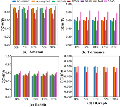
Figure 9. AUROC w.r.t. different anomaly contamination.

Appendix D Complexity Analysis

This subsection analyzes the time complexity of GGAD. We build a GCN to obtain the representation of each node, which takes $O(mdh)$, where $m$ is the number of non-zero elements in matrix $\bf A$ and $d$ is the dimension of representation and $h$ is the number of feature maps. The outliers are generated from the ego network of a labeled normal node, which will take $O(Skd^{2})$ where $S$ is the number of generated outliers and $k$ is the number of average neighbors for each outlier. The affinity calculation will take $O(N^{2}d)$, where $N$ is the number of nodes. The affinity separability and egocentric closeness constraints will take $O(N)$ and ${O(Sd)}$ respectively. The MLP layer mapping the representation to the anomaly score will take $O(Nd^{2})$. Thus, the overall complexity of GGAD is $O(mdh+Skd^{2}+N^{2}d+N+Sd+Nd^{2})$ (see Sec. 4.8 for empirical runtime results on CPU).

Appendix E Pseudo Codes of GGAD

The training algorithms of GGAD are summarized in Algorithm 2 and Algorithm 1. Algorithm 2 describes the full training process of GGAD. Algorithm 1 describes the mini-batch processing for handling very large graph datasets, i.e., DGraph. Since the number of the outlier nodes is significantly smaller than that of the normal nodes, we guarantee that each mini-batch consists of both normal and outlier nodes to address the potential data imbalanced problem. The outputs are the mini-batches of samples from the graph and corresponding structural information, which can then be used as the input of GGAD or the competing models to perform GAD on DGraph. Note that when using Algorithm 1 for the competing models, the steps that involve the generated outliers are not used if they do not have outlier generation components.

References

- (1)
- Bandyopadhyay et al. (2020) Sambaran Bandyopadhyay, Lokesh N, Saley Vishal Vivek, and M Narasimha Murty. 2020. Outlier resistant unsupervised deep architectures for attributed network embedding. In Proceedings of the 13th international conference on web search and data mining. 25–33.
- Cai et al. (2023) Jinyu Cai, Yunhe Zhang, and Jicong Fan. 2023. Self-Discriminative Modeling for Anomalous Graph Detection. arXiv preprint arXiv:2310.06261 (2023).
- Cao et al. (2024) Yunkang Cao, Xiaohao Xu, Jiangning Zhang, Yuqi Cheng, Xiaonan Huang, Guansong Pang, and Weiming Shen. 2024. A Survey on Visual Anomaly Detection: Challenge, Approach, and Prospect. arXiv preprint arXiv:2401.16402 (2024).
- Chai et al. (2022) Ziwei Chai, Siqi You, Yang Yang, Shiliang Pu, Jiarong Xu, Haoyang Cai, and Weihao Jiang. 2022. Can Abnormality be Detected by Graph Neural Networks. In Proceedings of the Twenty-Ninth International Joint Conference on Artificial Intelligence (IJCAI), Vienna, Austria. 23–29.
- Chen et al. (2020) Zhenxing Chen, Bo Liu, Meiqing Wang, Peng Dai, Jun Lv, and Liefeng Bo. 2020. Generative adversarial attributed network anomaly detection. In Proceedings of the 29th ACM International Conference on Information & Knowledge Management. 1989–1992.
- Ding et al. (2021) Kaize Ding, Jundong Li, Nitin Agarwal, and Huan Liu. 2021. Inductive anomaly detection on attributed networks. In Proceedings of the twenty-ninth international conference on international joint conferences on artificial intelligence. 1288–1294.
- Ding et al. (2019) Kaize Ding, Jundong Li, Rohit Bhanushali, and Huan Liu. 2019. Deep anomaly detection on attributed networks. In Proceedings of the 2019 SIAM International Conference on Data Mining. SIAM, 594–602.
- Dong et al. (2022) Linfeng Dong, Yang Liu, Xiang Ao, Jianfeng Chi, Jinghua Feng, Hao Yang, and Qing He. 2022. Bi-level selection via meta gradient for graph-based fraud detection. In International Conference on Database Systems for Advanced Applications. Springer, 387–394.
- Dou et al. (2020) Yingtong Dou, Zhiwei Liu, Li Sun, Yutong Deng, Hao Peng, and Philip S Yu. 2020. Enhancing graph neural network-based fraud detectors against camouflaged fraudsters. In Proceedings of the 29th ACM international conference on information & knowledge management. 315–324.
- Fan et al. (2020) Haoyi Fan, Fengbin Zhang, and Zuoyong Li. 2020. Anomalydae: Dual autoencoder for anomaly detection on attributed networks. In ICASSP 2020-2020 IEEE International Conference on Acoustics, Speech and Signal Processing (ICASSP). IEEE, 5685–5689.
- Gao et al. (2023a) Yuan Gao, Xiang Wang, Xiangnan He, Zhenguang Liu, Huamin Feng, and Yongdong Zhang. 2023a. Addressing heterophily in graph anomaly detection: A perspective of graph spectrum. In Proceedings of the ACM Web Conference 2023. 1528–1538.
- Gao et al. (2023b) Yuan Gao, Xiang Wang, Xiangnan He, Zhenguang Liu, Huamin Feng, and Yongdong Zhang. 2023b. Alleviating structural distribution shift in graph anomaly detection. In Proceedings of the Sixteenth ACM International Conference on Web Search and Data Mining. 357–365.
- Goodfellow et al. (2020) Ian Goodfellow, Jean Pouget-Abadie, Mehdi Mirza, Bing Xu, David Warde-Farley, Sherjil Ozair, Aaron Courville, and Yoshua Bengio. 2020. Generative adversarial networks. Commun. ACM 63, 11 (2020), 139–144.
- Huang et al. (2022a) Mengda Huang, Yang Liu, Xiang Ao, Kuan Li, Jianfeng Chi, Jinghua Feng, Hao Yang, and Qing He. 2022a. Auc-oriented graph neural network for fraud detection. In Proceedings of the ACM Web Conference 2022. 1311–1321.
- Huang et al. (2022b) Tianjin Huang, Yulong Pei, Vlado Menkovski, and Mykola Pechenizkiy. 2022b. Hop-count based self-supervised anomaly detection on attributed networks. In Joint European Conference on Machine Learning and Knowledge Discovery in Databases. Springer, 225–241.
- Huang et al. (2022c) Xuanwen Huang, Yang Yang, Yang Wang, Chunping Wang, Zhisheng Zhang, Jiarong Xu, Lei Chen, and Michalis Vazirgiannis. 2022c. Dgraph: A large-scale financial dataset for graph anomaly detection. Advances in Neural Information Processing Systems 35 (2022), 22765–22777.
- Jiang et al. (2023) Minqi Jiang, Chaochuan Hou, Ao Zheng, Songqiao Han, Hailiang Huang, Qingsong Wen, Xiyang Hu, and Yue Zhao. 2023. ADGym: Design Choices for Deep Anomaly Detection. In Thirty-seventh Conference on Neural Information Processing Systems Datasets and Benchmarks Track.
- Kinga et al. (2015) D Kinga, Jimmy Ba Adam, et al. 2015. A method for stochastic optimization. In International conference on learning representations (ICLR), Vol. 5. San Diego, California;, 6.
- Kumar et al. (2019) Srijan Kumar, Xikun Zhang, and Jure Leskovec. 2019. Predicting dynamic embedding trajectory in temporal interaction networks. In Proceedings of the 25th ACM SIGKDD international conference on knowledge discovery & data mining. 1269–1278.
- Li et al. (2017) Jundong Li, Harsh Dani, Xia Hu, and Huan Liu. 2017. Radar: Residual Analysis for Anomaly Detection in Attributed Networks.. In IJCAI. 2152–2158.
- Liu et al. (2022a) Kay Liu, Yingtong Dou, Yue Zhao, Xueying Ding, Xiyang Hu, Ruitong Zhang, Kaize Ding, Canyu Chen, Hao Peng, Kai Shu, George H. Chen, Zhihao Jia, and Philip S. Yu. 2022a. PyGOD: A Python Library for Graph Outlier Detection. arXiv preprint arXiv:2204.12095 (2022).
- Liu et al. (2022b) Kay Liu, Yingtong Dou, Yue Zhao, Xueying Ding, Xiyang Hu, Ruitong Zhang, Kaize Ding, Canyu Chen, Hao Peng, Kai Shu, Lichao Sun, Jundong Li, George H. Chen, Zhihao Jia, and Philip S. Yu. 2022b. Bond: Benchmarking unsupervised outlier node detection on static attributed graphs. Advances in Neural Information Processing Systems 35 (2022), 27021–27035.
- Liu et al. (2021a) Yang Liu, Xiang Ao, Zidi Qin, Jianfeng Chi, Jinghua Feng, Hao Yang, and Qing He. 2021a. Pick and choose: a GNN-based imbalanced learning approach for fraud detection. In Proceedings of the web conference 2021. 3168–3177.
- Liu et al. (2023a) Yixin Liu, Kaize Ding, Qinghua Lu, Fuyi Li, Leo Yu Zhang, and Shirui Pan. 2023a. Towards Self-Interpretable Graph-Level Anomaly Detection. arXiv preprint arXiv:2310.16520 (2023).
- Liu et al. (2021b) Yixin Liu, Zhao Li, Shirui Pan, Chen Gong, Chuan Zhou, and George Karypis. 2021b. Anomaly detection on attributed networks via contrastive self-supervised learning. IEEE transactions on neural networks and learning systems 33, 6 (2021), 2378–2392.
- Liu et al. (2023b) Zuhao Liu, Xiao-Ming Wu, Dian Zheng, Kun-Yu Lin, and Wei-Shi Zheng. 2023b. Generating Anomalies for Video Anomaly Detection With Prompt-Based Feature Mapping. In Proceedings of the IEEE/CVF Conference on Computer Vision and Pattern Recognition. 24500–24510.
- Ma et al. (2022) Rongrong Ma, Guansong Pang, Ling Chen, and Anton van den Hengel. 2022. Deep graph-level anomaly detection by glocal knowledge distillation. In Proceedings of the Fifteenth ACM International Conference on Web Search and Data Mining. 704–714.
- Ma et al. (2021) Xiaoxiao Ma, Jia Wu, Shan Xue, Jian Yang, Chuan Zhou, Quan Z Sheng, Hui Xiong, and Leman Akoglu. 2021. A comprehensive survey on graph anomaly detection with deep learning. IEEE Transactions on Knowledge and Data Engineering (2021).
- Ma et al. (2023) Xiaoxiao Ma, Jia Wu, Jian Yang, and Quan Z Sheng. 2023. Towards graph-level anomaly detection via deep evolutionary mapping. In Proceedings of the 29th ACM SIGKDD Conference on Knowledge Discovery and Data Mining. 1631–1642.
- Meng et al. (2023) Lin Meng, Hesham Mostafa, Marcel Nassar, Xiaonan Zhang, and Jiawei Zhang. 2023. Generative Graph Augmentation for Minority Class in Fraud Detection. In Proceedings of the 32nd ACM International Conference on Information and Knowledge Management. 4200–4204.
- Ngo et al. (2019) Phuc Cuong Ngo, Amadeus Aristo Winarto, Connie Khor Li Kou, Sojeong Park, Farhan Akram, and Hwee Kuan Lee. 2019. Fence GAN: Towards better anomaly detection. In 2019 IEEE 31St International Conference on tools with artificial intelligence (ICTAI). IEEE, 141–148.
- Niu et al. (2023) Chaoxi Niu, Guansong Pang, and Ling Chen. 2023. Graph-level anomaly detection via hierarchical memory networks. In Joint European Conference on Machine Learning and Knowledge Discovery in Databases. Springer, 201–218.
- Pang et al. (2021a) Guansong Pang, Chunhua Shen, Longbing Cao, and Anton Van Den Hengel. 2021a. Deep learning for anomaly detection: A review. ACM computing surveys (CSUR) 54, 2 (2021), 1–38.
- Pang et al. (2021b) Guansong Pang, Anton van den Hengel, Chunhua Shen, and Longbing Cao. 2021b. Toward deep supervised anomaly detection: Reinforcement learning from partially labeled anomaly data. In Proceedings of the 27th ACM SIGKDD conference on knowledge discovery & data mining. 1298–1308.
- Park et al. (2022) Joonhyung Park, Jaeyun Song, and Eunho Yang. 2022. Graphens: Neighbor-aware ego network synthesis for class-imbalanced node classification. In The Tenth International Conference on Learning Representations, ICLR 2022. International Conference on Learning Representations (ICLR).
- Peng et al. (2018) Zhen Peng, Minnan Luo, Jundong Li, Huan Liu, and Qinghua Zheng. 2018. ANOMALOUS: A Joint Modeling Approach for Anomaly Detection on Attributed Networks.. In IJCAI. 3513–3519.
- Perozzi and Akoglu (2016) Bryan Perozzi and Leman Akoglu. 2016. Scalable anomaly ranking of attributed neighborhoods. In Proceedings of the 2016 SIAM International Conference on Data Mining. SIAM, 207–215.
- Qiao and Pang (2023) Hezhe Qiao and Guansong Pang. 2023. Truncated Affinity Maximization: One-class Homophily Modeling for Graph Anomaly Detection. In Advances in Neural Information Processing Systems.
- Roy et al. (2024) Amit Roy, Juan Shu, Jia Li, Carl Yang, Olivier Elshocht, Jeroen Smeets, and Pan Li. 2024. GAD-NR : Graph Anomaly Detection via Neighborhood Reconstruction. In Proceedings of the 17th ACM International Conference on Web Search and Data Mining.
- Sabokrou et al. (2021) Mohammad Sabokrou, Mahmood Fathy, Guoying Zhao, and Ehsan Adeli. 2021. Deep End-to-End One-Class Classifier. IEEE transactions on neural networks and learning systems 32, 2 (2021), 675–684.
- Shi et al. (2022) Fengzhao Shi, Yanan Cao, Yanmin Shang, Yuchen Zhou, Chuan Zhou, and Jia Wu. 2022. H2-fdetector: A gnn-based fraud detector with homophilic and heterophilic connections. In Proceedings of the ACM Web Conference 2022. 1486–1494.
- Tang et al. (2023) Jianheng Tang, Fengrui Hua, Ziqi Gao, Peilin Zhao, and Jia Li. 2023. GADBench: Revisiting and Benchmarking Supervised Graph Anomaly Detection. arXiv preprint arXiv:2306.12251 (2023).
- Tang et al. (2022) Jianheng Tang, Jiajin Li, Ziqi Gao, and Jia Li. 2022. Rethinking graph neural networks for anomaly detection. In International Conference on Machine Learning. PMLR, 21076–21089.
- Wang et al. (2023a) Qizhou Wang, Guansong Pang, Mahsa Salehi, Wray Buntine, and Christopher Leckie. 2023a. Cross-domain graph anomaly detection via anomaly-aware contrastive alignment. In Proceedings of the AAAI Conference on Artificial Intelligence, Vol. 37. 4676–4684.
- Wang et al. (2023b) Qizhou Wang, Guansong Pang, Mahsa Salehi, Wray Buntine, and Christopher Leckie. 2023b. Open-Set Graph Anomaly Detection via Normal Structure Regularisation. arXiv preprint arXiv:2311.06835 (2023).
- Wang et al. (2021) Xuhong Wang, Baihong Jin, Ying Du, Ping Cui, Yingshui Tan, and Yupu Yang. 2021. One-class graph neural networks for anomaly detection in attributed networks. Neural computing and applications 33 (2021), 12073–12085.
- Wang et al. (2023c) Yuchen Wang, Jinghui Zhang, Zhengjie Huang, Weibin Li, Shikun Feng, Ziheng Ma, Yu Sun, Dianhai Yu, Fang Dong, Jiahui Jin, et al. 2023c. Label Information Enhanced Fraud Detection against Low Homophily in Graphs. In Proceedings of the ACM Web Conference 2023. 406–416.
- Xu et al. (2023) Hongzuo Xu, Guansong Pang, Yijie Wang, and Yongjun Wang. 2023. Deep isolation forest for anomaly detection. IEEE Transactions on Knowledge and Data Engineering (2023).
- Yang et al. (2023) Yiyuan Yang, Chaoli Zhang, Tian Zhou, Qingsong Wen, and Liang Sun. 2023. DCdetector: Dual Attention Contrastive Representation Learning for Time Series Anomaly Detection. In Proceedings of the 28th ACM SIGKDD Conference on Knowledge Discovery and Data Mining.
- Zaheer et al. (2022) M Zaigham Zaheer, Arif Mahmood, M Haris Khan, Mattia Segu, Fisher Yu, and Seung-Ik Lee. 2022. Generative cooperative learning for unsupervised video anomaly detection. In Proceedings of the IEEE/CVF conference on computer vision and pattern recognition. 14744–14754.
- Zenati et al. (2018) Houssam Zenati, Manon Romain, Chuan-Sheng Foo, Bruno Lecouat, and Vijay Chandrasekhar. 2018. Adversarially learned anomaly detection. In 2018 IEEE International conference on data mining (ICDM). IEEE, 727–736.
- Zhang et al. (2022b) Chaoli Zhang, Tian Zhou, Qingsong Wen, and Liang Sun. 2022b. TFAD: A decomposition time series anomaly detection architecture with time-frequency analysis. In Proceedings of the 31st ACM International Conference on Information & Knowledge Management. 2497–2507.
- Zhang et al. (2021) Ge Zhang, Jia Wu, Jian Yang, Amin Beheshti, Shan Xue, Chuan Zhou, and Quan Z Sheng. 2021. Fraudre: Fraud detection dual-resistant to graph inconsistency and imbalance. In 2021 IEEE International Conference on Data Mining (ICDM). IEEE, 867–876.
- Zhang et al. (2022a) Ge Zhang, Zhenyu Yang, Jia Wu, Jian Yang, Shan Xue, Hao Peng, Jianlin Su, Chuan Zhou, Quan Z Sheng, Leman Akoglu, et al. 2022a. Dual-discriminative graph neural network for imbalanced graph-level anomaly detection. Advances in Neural Information Processing Systems 35 (2022), 24144–24157.
- Zhang et al. (2023) Zhijie Zhang, Wenzhong Li, Wangxiang Ding, Linming Zhang, Qingning Lu, Peng Hu, Tong Gui, and Sanglu Lu. 2023. STAD-GAN: unsupervised anomaly detection on multivariate time series with self-training generative adversarial networks. ACM Transactions on Knowledge Discovery from Data 17, 5 (2023), 1–18.
- Zheng et al. (2019) Panpan Zheng, Shuhan Yuan, Xintao Wu, Jun Li, and Aidong Lu. 2019. One-class adversarial nets for fraud detection. In Proceedings of the AAAI Conference on Artificial Intelligence, Vol. 33. 1286–1293.
- Zheng et al. (2021) Yu Zheng, Ming Jin, Yixin Liu, Lianhua Chi, Khoa T Phan, and Yi-Ping Phoebe Chen. 2021. Generative and contrastive self-supervised learning for graph anomaly detection. IEEE Transactions on Knowledge and Data Engineering (2021).
- Zhu et al. (2020) Yanqiao Zhu, Yichen Xu, Feng Yu, Qiang Liu, Shu Wu, and Liang Wang. 2020. Deep graph contrastive representation learning. arXiv preprint arXiv:2006.04131 (2020).
- Zhuang et al. (2023) Zhong Zhuang, Kai Ming Ting, Guansong Pang, and Shuaibin Song. 2023. Subgraph Centralization: A Necessary Step for Graph Anomaly Detection. In Proceedings of the 2023 SIAM International Conference on Data Mining (SDM). SIAM, 703–711.