Finite-Time Error Analysis of Online Model-Based Q-Learning with a Relaxed Sampling Model

Abstract

Reinforcement learning has witnessed significant advancements, particularly with the emergence of model-based approaches. Among these, $Q$-learning has proven to be a powerful algorithm in model-free settings. However, the extension of $Q$-learning to a model-based framework remains relatively unexplored. In this paper, we delve into the sample complexity of $Q$-learning when integrated with a model-based approach. Through theoretical analyses and empirical evaluations, we seek to elucidate the conditions under which model-based $Q$-learning excels in terms of sample efficiency compared to its model-free counterpart.

1 Introduction

Reinforcement learning (RL) aims to solve a sequential decision making problem. In a broad perspective, RL algorithms can be categorized into two classes: model-free and model-based approach. Both methods have shown great success in various scenarios [Silver et al., 2017, Fawzi et al., 2022]. The model-free approach tries to solve the sequential decision making process without any knowledge of a model. In contrast, the model-based approach leverages a known or estimated model during the learning process.

$Q$-learning, developed by Watkins and Dayan [1992], is one of the most widely used model-free RL algorithms. A rich body of literature has tried to understand the nature of $Q$-learning, and its non-asymptotic behavior has been recently understood in detail [Qu and Wierman, 2020, Chen et al., 2019, Lee, 2022, Li et al., 2023]. In particular, Li et al. [2023] proved a tight sample complexity bound of $Q$-learning, which matches the lower bound on the sample complexity of $Q$-learning.

Meanwhile, a natural method to improve the sample efficiency of RL algorithms is to incorporate the model into the learning phase. Both in theoretical and experimental sense, leveraging the knowledge of learned or known model has been shown to improve over the model-free methods. For instance, Nagabandi et al. [2018], Chua et al. [2018], Kidambi et al. [2020] experimentally verified that approximating a model improves the sample efficiency of model-free algorithms. The sample efficiency of model-based algorithms has been studied in Kearns and Singh [2002], Azar et al. [2012] under various settings in theoretical manners.

An intuitive method to extend $Q$-learning to a model-based approach, is to replace the stochastic components in the $Q$-learning update with estimators calculated via previous samples. In this paper, we study to what extent, we can improve the $Q$-learning with a model-based approach. We consider a natural extension of $Q$-learning with estimated model, which we call synchronous model-based $Q$-learning (SyncMBQ). In this respect, our main contributions are summarized as follows:

1. We consider a new model-based RL algorithm, called SyncMBQ, which is an extension of $Q$-learning to model-based approaches, and prove its near-optimal sample complexity under a general step-size regime, $\alpha\in(0,1)$.

2. SyncMBQ can be seen as an online model-based $Q$-learning, where the model estimate and $Q$-estimate are learned simultaneously in an online manner. It is online because the model and $Q$-estimate are updated in real-time using a single transition of the system at each iteration.

3. Moreover, SyncMBQ uses a more relaxed sampling model compared to the idealistic generative models (sampling oracle) used in some of previous model-based RLs. In particular, SyncMBQ uses a single transition at each iteration, where only one state-action pair is sampled from a fixed distribution under an exploratory behavior policy, and then the corresponding next state is sampled. This scenario is obviously weaker than the generative model cases.

4. To the authors’ knowledge, SyncMBQ considered in this paper has not been considered and thoroughly investigated so far in the literature. In this paper, we prove that SyncMBQ can achieve $\tilde{{\mathcal{O}}}\left(\frac{|{\mathcal{S}}||{\mathcal{A}}|}{(1-\gamma)^{4}{\epsilon}^{2}}\right)$ sample complexity, which is compatible with the optimal sample complexity $\tilde{{\mathcal{O}}}\left(\frac{|{\mathcal{S}}||{\mathcal{A}}|}{(1-\gamma)^{3}{\epsilon}^{2}}\right)$ achievable by existing model-based RLs with generative models except for the order of the effective horizon $\frac{1}{1-\gamma}$. Moreover, this result improves the sample complexities achievable by existing model-based RLs without relying on generative models. Note also that this sample complexity is identical to the optimal sample complexity (not improvable) reported in Li et al. [2023] for a model-free $Q$-learning with a restrictive step-size regime. SyncMBQ can achieve an identical efficiency under more general step-size regimes.

5. For the analysis, the recenty developed switching system model framework in Lee [2022] is adopted in this paper. However, we develop a new switching system model for SyncMBQ and use it for our finite-time analysis. Finally, the performance of SyncMBQ is demonstrated via simulations, which empirically verify that SyncMBQ outperforms $Q$-learning under various scenarios.

Related Works on model-free Q-learning: Recently, some advances have been made on the non-asymptotic behavior of model-free $Q$-learning algorithms [Chen et al., 2019, Qu and Wierman, 2020, Lee, 2022, Li et al., 2023]. For example, Chen et al. [2019], Qu and Wierman [2020], Lee [2022] studied asynchronous $Q$-learning, where only the $Q$-function estimate corresponding to a single state-action pair is updated at each iteration. Moreover, Li et al. [2023] proved that synchronous $Q$-learning, which updates the $Q$-function estimate for every state-action pairs each iteration, requires $\tilde{{\mathcal{O}}}\left(\frac{|{\mathcal{S}}||{\mathcal{A}}|}{(1-\gamma)^{4}{\epsilon}^{2}}\right)$ number of samples, which matches the known lower bound of the sample complexity of $Q$-learning.

Related works on model-based Q-learning: Model-based RL algorithms have been studied in Azar et al. [2012], Gheshlaghi Azar et al. [2013], Li et al. [2020], Agarwal et al. [2020] under the assumption that generative models are available, where a generative model means a sampling oracle where we can access any state-action pair in the environment on our choice and get the next state. Roughly speaking, the main idea of these works is to run a $Q$-value iteration with the transition matrix and reward function replaced with the corresponding estimated models learned through the generative models. In particular, Azar et al. [2012], Gheshlaghi Azar et al. [2013], Li et al. [2020], Agarwal et al. [2020] proposed model-based algorithms which consist of the two phases: in the first phase, the model is learned through samples from generative models; in the second phase, dynamic programmings are applied using the learned model. The authors of Azar et al. [2012] established a lower bound of $\tilde{{\mathcal{O}}}\left(\frac{|{\mathcal{S}}||{\mathcal{A}}|}{(1-\gamma)^{3}{\epsilon}^{2}}\right)$ on the sample complexity inherent to all RL algorithms and demonstrated that the sample complexity of their algorithm aligns with this established lower bound when a sufficient number of samples are collected in the first phase. More recently, Li et al. [2020] derived a similar sample complexity $\tilde{{\mathcal{O}}}\left(\frac{|{\mathcal{S}}||{\mathcal{A}}|}{(1-\gamma)^{3}{\epsilon}^{2}}\right)$, and Agarwal et al. [2020] theoretically studied the optimality of these model-based $Q$-learning algorithms based on generative models.

Batch $Q$-learning algorithms, which use a number of samples collected at each iteration to construct an approximate Bellman operator, can be also interpreted as a non-parametric model-based $Q$-learning. Relying on an empirical mean estimator of the Bellman operator makes similar effect as leveraging a model estimate while reducing the space complexity from ${\mathcal{O}}(|{\mathcal{S}}|^{2}|{\mathcal{A}}|)$ to ${\mathcal{O}}\left(|{\mathcal{S}}||{\mathcal{A}}|\right)$. For example, Kearns and Singh [1998], Kalathil et al. [2021], Wainwright [2019] studied empirical $Q$-value iteration algorithms, which estimate empirical Bellman operator with newly collected samples from a generative model at every iteration. In particular, Kearns and Singh [1998] investigated the so-called phased $Q$-learning that uses estimated transition matrix estimated with newly collected samples at each iteration using the generative model. Phased $Q$-learning has been proven to achieve $\tilde{{\mathcal{O}}}\left(\frac{|{\mathcal{S}}||{\mathcal{A}}|}{(1-\gamma)^{4}{\epsilon}^{2}}\right)$ sample complexity. This algorithm includes both a non-parametric batch version of $Q$-learning and a parametric model-based $Q$-learning version. In Kalathil et al. [2021], the authors proved that their empirical $Q$-value iteration can have $\tilde{{\mathcal{O}}}\left(\frac{|{\mathcal{S}}||{\mathcal{A}}|}{(1-\gamma)^{4}{\epsilon}^{2}}\right)$ sample complexity to achieve desired level of accuracy. Moreover, Sidford et al. [2018] proposed a slightly different variance-reduced $Q$-value iteration algorithm and obtained $\tilde{{\mathcal{O}}}\left(\frac{|{\mathcal{S}}||{\mathcal{A}}|}{(1-\gamma)^{3}{\epsilon}^{2}}\right)$ sample complexities. Afterwards, Wainwright [2019] developed a variance-reduced $Q$-learning (a batch $Q$-learning), and proved that it can also achieve the optimal sample complexity $\tilde{{\mathcal{O}}}\left(\frac{|{\mathcal{S}}||{\mathcal{A}}|}{(1-\gamma)^{3}{\epsilon}^{2}}\right)$. Note that all the aforementioned approaches require an access to a generative model, which is one of the most idealistic scenarios. The so-called delayed $Q$-learning, introduced by Strehl et al. [2006], is also a batch $Q$-learning algorithm, which can be seen as a non-parametric model-based $Q$-learning. It has been proved that the delayed $Q$-learning can achieve $\tilde{{\mathcal{O}}}\left(\frac{|{\mathcal{S}}||{\mathcal{A}}|}{(1-\gamma)^{7}{\epsilon}^{4}}\right)$ sample complexity, while it does not require a generative model, and uses samples from a single trajectory.

Without relying on generative models, more practical model-based RL algorithms have been studied in Kearns and Singh [2002], Brafman and Tennenholtz [2002], Strehl and Littman [2005], Szita and Szepesvári [2010] with corresponding sample complexities, where explorations and single trajectory-based samples are used. In particular, Kearns and Singh [2002] proposed the so-called $E^{3}$ algorithm which decides to explore or exploit relying on the estimated model, and Brafman and Tennenholtz [2002] introduced the so-called R-max algorithm wherein an agent acts by an optimal policy derived from the estimated model, and requires $\tilde{{\mathcal{O}}}\left(\frac{|{\mathcal{S}}|^{2}|{\mathcal{A}}|}{(1-\gamma)^{6}{\epsilon}^{3}}\right)$ number of samples. In a subsequent work, Szita and Szepesvári [2010] proposed a modified version of R-max algorithm that achieves $\tilde{{\mathcal{O}}}\left(\frac{|{\mathcal{S}}||{\mathcal{A}}|}{(1-\gamma)^{6}{\epsilon}^{2}}\right)$ sample complexity. Moreover, Strehl and Littman [2005] used a model based interval estimation method [Wiering and Schmidhuber, 1998] to deal with the exploration-exploitation dilemma and proved that it can also achieve $\tilde{{\mathcal{O}}}\left(\frac{|{\mathcal{S}}|^{2}|{\mathcal{A}}|}{(1-\gamma)^{6}{\epsilon}^{3}}\right)$ sample complexity. In Lattimore and Hutter [2014], the authors studied the so-called UCRL$\gamma$ algorithm that achieves $\tilde{{\mathcal{O}}}\left(\frac{|{\mathcal{S}}|^{2}|{\mathcal{A}}|}{(1-\gamma)^{3}{\epsilon}^{2}}\right)$ sample complexity, which is optimal in terms of the effective horizon $\frac{1}{1-\gamma}$, while sub-optimal in terms of the state size $|{\cal S}|$.

Lastly, we note that Gheshlaghi Azar et al. [2013], Sidford et al. [2018], Li et al. [2020], Agarwal et al. [2020] studied sample complexities to obtain ${\epsilon}$-optimal policy. In this work, we focus on the sample complexity to obtain the ${\epsilon}$-optimal value function rather than ${\epsilon}$-optimal policy.

2 Preliminaries

2.1 Markov decision process

A Markov decision process (MDP) consists of five tuples $({\mathcal{S}},{\mathcal{A}},\gamma,{\mathcal{P}},{\mathcal{R}})$ where ${\mathcal{S}}:=\{1,2,\dots,|{\mathcal{S}}|\}$ is the collection of states, ${\mathcal{A}}:=\{1,2,\dots,|{\mathcal{A}}|\}$ is the collection of actions, $\gamma\in(0,1)$ is the discount factor, ${\mathcal{P}}:{\mathcal{S}}\times{\mathcal{A}}\times{\mathcal{S}}\to[0,1]$ is the transition kernel, and ${\mathcal{R}}:{\mathcal{S}}\times{\mathcal{A}}\times{\mathcal{S}}\to\mathbb{R}$ is the reward function. Upon taking action $a\in{\mathcal{A}}$ at state $s\in{\mathcal{S}}$, transition to $s^{\prime}\in{\mathcal{S}}$ occurs with probability ${\mathcal{P}}(s,a,s^{\prime})$ and reward ${\mathcal{R}}(s,a,s^{\prime})$ is incurred. For simplicity of the proof, we assume that the reward function is bounded, i.e., $|{\mathcal{R}}(s,a,s^{\prime})|\leq 1$ for all $(s,a,s^{\prime})\in{\mathcal{S}}\times{\mathcal{A}}\times{\mathcal{S}}$.

A deterministic policy $\pi:{\mathcal{S}}\to{\mathcal{A}}$ maps a state $s\in{\mathcal{S}}$ to an action $a\in{\mathcal{A}}$. We study finding an optimal deterministic policy, $\pi^{*}$, that maximizes the expected sum of discounted rewards under an infinite horizon MDP setting, i.e.,

$$\pi^{*}:=\operatorname*{arg\,max}_{\pi\in\Omega}\sum_{k=0}^{\infty}\mathbb{E}\left[\gamma^{k}r_{k}\middle|\pi\right],$$

where $\Omega$ is the set of all admissible deterministic policies, $r_{k}:={\mathcal{R}}(s_{k},a_{k},s_{k+1})$, $\{(s_{k},a_{k})\in{\mathcal{S}}\times{\mathcal{A}}\}_{k\in{\mathbb{N}}}$ is a sequence of state-action trajectory generated by a Markov decision process under policy $\pi$, and $\mathbb{E}\left[\cdot\middle|\pi\right]$ denotes the expected value conditioned on policy $\pi$. The $Q$-function under policy $\pi$, $Q^{\pi}:{\mathcal{S}}\times{\mathcal{A}}\to\mathbb{R}$, denotes expected cumulative discounted reward starting at $(s,a)\in{\mathcal{S}}\times{\mathcal{A}}$ and following policy $\pi$ afterwards:

$$Q^{\pi}(s,a):=\sum^{\infty}_{k=0}\mathbb{E}\left[\gamma^{k}r_{k}\middle|(s_{0},a_{0})=(s,a),\;\pi\right].$$

The optimal $Q$-function, which is a $Q$-function induced by the optimal policy $\pi^{*}$, is denoted as $Q^{*}(s,a):=Q^{\pi^{*}}(s,a)$ for all $s,a\in{\mathcal{S}}\times{\mathcal{A}}$. The optimal policy $\pi^{*}$ can be recovered once $Q^{*}$ is known, i.e., $\pi^{*}(s)=\operatorname*{arg\,max}_{a\in{\mathcal{A}}}Q^{*}(s,a)$. It is well known that the optimal $Q$-function, $Q^{*}$, satisfies the following equation, the so-called optimal Bellman equation [Bellman, 1966], for all $s\in{\mathcal{S}},a\in{\mathcal{A}}$:

$$Q^{*}(s,a)=\sum_{s^{\prime}\in{\mathcal{S}}}{\mathcal{P}}(s,a,s^{\prime})\left({\mathcal{R}}(s,a,s^{\prime})+\gamma\max_{u\in{\mathcal{A}}}Q^{*}(s,u)\right).$$

2.2 Overview of Q-learning

In this section, we briefly illustrate the $Q$-learning algorithm [Watkins and Dayan, 1992]. The $Q$-learning algorithm is one of the well-known model-free algorithms. The update of $Q$-learning can be written as, for $k\in{\mathbb{N}}$, and ${\bm{Q}}_{0}\in\mathbb{R}^{|{\mathcal{S}}||{\mathcal{A}}|}$:

$${\bm{Q}}_{k+1}(s_{k},a_{k})= (1-\alpha){\bm{Q}}_{k}(s_{k},a_{k})$$

$$+\alpha\left(r_{k}+\gamma\max_{a\in{\mathcal{A}}}{\bm{Q}}_{k}(s_{k+1},a)\right),$$ (1)

where ${\bm{Q}}_{k}\in\mathbb{R}^{|{\mathcal{S}}||{\mathcal{A}}|}$, ${\bm{Q}}_{k}(s,a)=({\bm{e}}_{s}\otimes{\bm{e}}_{a})^{\top}{\bm{Q}}_{k}$ for $(s,a)\in{\mathcal{S}}\times{\mathcal{A}}$, $\alpha\in(0,1)$ is the constant step-size, and ${\bm{e}}_{s}$ and ${\bm{e}}_{a}$ denote $s$-th and $a$-th canonical basis vectors in $\mathbb{R}^{|{\mathcal{S}}|}$ and $\mathbb{R}^{|{\mathcal{A}}|}$, respectively.

To proceed, we further assume that at time step $k$, the state-action pair $(s_{k},a_{k})$ is sampled from a fixed probability $d:{\mathcal{S}}\times{\mathcal{A}}\to[0,1]$. We will assume that $d(s,a)>0$ for all $s,a\in{\mathcal{S}}\times{\mathcal{A}}$, and let $d_{\min}:=\min_{s,a\in{\mathcal{S}}\times{\mathcal{A}}}d(s,a)$. Furthermore, we introduce a set of matrix notations:

$${\bm{P}}:= \begin{bmatrix}{\bm{p}}^{1,1}&{\bm{p}}^{1,2}&\cdots&{\bm{p}}^{|{\mathcal{S}}|,|{\mathcal{A}}|}\end{bmatrix}^{\top}\in\mathbb{R}^{|{\mathcal{S}}||{\mathcal{A}}|\times|{\mathcal{S}}|},$$

$${\bm{R}}:= \begin{bmatrix}{\bm{R}}^{1,1}&{\bm{R}}^{1,2}&\cdots&{\bm{R}}^{|{\mathcal{S}}|,|{\mathcal{A}}|}\end{bmatrix}^{\top}\in\mathbb{R}^{|{\mathcal{S}}||{\mathcal{A}}|},$$

$${\bm{D}}:= \begin{bmatrix}d(1,1)&&\\ &\ddots&\\ &&d(|{\mathcal{S}}|,|{\mathcal{A}}|)\end{bmatrix}\in\mathbb{R}^{|{\mathcal{S}}||{\mathcal{A}}|\times|{\mathcal{S}}||{\mathcal{A}}|},$$

where ${\bm{p}}^{s,a}\in\mathbb{R}^{|{\mathcal{S}}|}$ is a column vector whose $s^{\prime}$-th element corresponds to ${\mathcal{P}}(s,a,s^{\prime})$ for $s^{\prime}\in{\mathcal{S}}$, and ${\bm{R}}^{s,a}:=\mathbb{E}\left[r(s,a,s^{\prime})\middle|s,a\right]$. Moreover, for any deterministic policy $\pi:{\mathcal{S}}\to{\mathcal{A}}$, define,

$${\bm{\Pi}}^{\pi}:=\begin{bmatrix}{\bm{e}}_{1}^{\top}\otimes{\bm{\pi}}(1)^{\top}\\ {\bm{e}}_{2}^{\top}\otimes{\bm{\pi}}(2)^{\top}\\ \vdots\\ {\bm{e}}_{|{\mathcal{S}}|}^{\top}\otimes{\bm{\pi}}(|{\mathcal{S}}|)^{\top}\end{bmatrix}\in\mathbb{R}^{|{\mathcal{S}}|\times|{\mathcal{S}}||{\mathcal{A}}|},$$

where ${\bm{e}}_{s}\in\mathbb{R}^{|{\mathcal{S}}|}$ for $s\in{\mathcal{S}}$ denotes the basis vector in $\mathbb{R}^{|{\mathcal{S}}|}$ whose $s$-th element is one and others are zero, and ${\bm{\pi}}(s)\in\mathbb{R}^{|{\mathcal{A}}|}$ is a column vector whose $\pi(s)$-th element is one and others are all zero. We will denote the greedy policy induced by ${\bm{Q}}\in\mathbb{R}^{|{\mathcal{S}}||{\mathcal{A}}|}$, as $\pi_{{\bm{Q}}}(s):=\operatorname*{arg\,max}_{a\in{\mathcal{A}}}{\bm{Q}}(s,a)$ where ${\bm{Q}}(s,a)=({\bm{e}}_{s}\otimes{\bm{e}}_{a})^{\top}{\bm{Q}}$, for $s\in{\mathcal{S}}$, and let ${\bm{\Pi}}^{{\bm{Q}}}:={\bm{\Pi}}^{\pi_{{\bm{Q}}}}$.

2.3 Switched system theory

In this section, a brief overview of the switching system [Liberzon, 2005] is given. A switched system viewpoint has been a useful tool to analyze the behavior of $Q$-learning [Lee and He, 2019]. The state variable ${\bm{x}}_{k}\in\mathbb{R}^{n},k\in{\mathbb{N}}$ of a switched affine system evolves via the following equation:

$${\bm{x}}_{k+1}={\bm{A}}_{\sigma(k)}{\bm{x}}_{k}+{\bm{b}}_{\sigma(k)},\quad{\bm{x}}_{0}\in\mathbb{R}^{n}$$

where $\sigma\in{\mathcal{M}}:\{1,2,\dots,|{\mathcal{M}}|\}$ is called the mode, $\sigma(k)\in{\mathcal{M}}$ is the switching signal, $\{{\bm{A}}_{\sigma}\in\mathbb{R}^{n\times n};\sigma\in{\mathcal{M}}\}$ and $\{{\bm{b}}_{\sigma}\in\mathbb{R}^{n};\sigma\in{\mathcal{M}}\}$ are the subsystem matrices and vectors, respectively. The switching signal can be either determined arbitrary or controlled by a particular logic. When ${\bm{b}}_{\sigma}$, the so-called affine term, is zero vector for any $\sigma\in{\mathcal{M}}$, the above system is called the switched linear system.

3 Synchronous Model-based Q-learning

In this section, we first explicitly state the SyncMBQ in Algorithm 1 studied in this paper, and provide its sample complexity. We begin by introducing the estimators for the transition matrix and reward function.

Algorithm 1 Synchronous Model-based Q-learning (SyncMBQ)

1:Initialize $\alpha\in(0,1),\;{\bm{Q}}_{1}={\bm{Q}}_{2}=\dots={\bm{Q}}_{m}\in\mathbb{R}^{|{\mathcal{S}}||{\mathcal{A}}|},\;\hat{{\bm{P}}}_{0}=\bm{0},\;\hat{{\bm{R}}}_{0}=\bm{0}$.

2:for $k=1,2,\dots,m$ do

3:     Observe $s_{k},a_{k},s^{\prime}_{k}$ and $r_{k}:=r(s_{k},a_{k},s^{\prime}_{k})$

4:     Update $\hat{{\bm{P}}}_{k}$ and $\hat{{\bm{R}}}_{k}$ following (4) and (5), respectively.

5:     Update $N_{k}^{s_{k}a_{k}}=N_{k-1}^{s_{k}a_{k}}+1$.

6:end for

7:for $k=m+1,m+2,\dots,$ do

8:     Observe $s_{k},a_{k},s^{\prime}_{k}$ and $r_{k}:=r(s_{k},a_{k},s^{\prime}_{k})$ where $s_{k},a_{k}\sim d(\cdot)$ and $s_{k}^{\prime}\sim{\mathcal{P}}(\cdot\mid s_{k},a_{k})$.

9:     Update $\hat{{\bm{P}}}_{k}$ and $\hat{{\bm{R}}}_{k}$ following (4) and (5), respectively.

10:     Update ${\bm{Q}}_{k}$:

$${\bm{Q}}_{k+1}={\bm{Q}}_{k}+\alpha(\hat{{\bm{R}}}_{k}+\gamma\hat{{\bm{P}}}_{k}{\bm{\Pi}}_{{\bm{Q}}_{k}}{\bm{Q}}_{k}-{\bm{Q}}_{k})$$ (2)

11:     Update $N_{k}^{s_{k},a_{k}}=N_{k-1}^{s_{k},a_{k}}+1$.

12:end for

3.1 Model-based approach

The model-based approach maintains statistical estimators of the transition probability ${\mathcal{P}}(s,a,s^{\prime})$, denoted by $\hat{p}^{s,a,s^{\prime}}_{k}$, and expected reward $\mathbb{E}[{\mathcal{R}}(s,a,s^{\prime})\mid s,a]$, denoted by $\hat{r}^{s,a}_{k}$, at time step $k\in{\mathbb{N}}$ and for all $(s,a,s^{\prime})\in{\mathcal{S}}\times{\mathcal{A}}\times{\mathcal{S}}$. We can naturally incorporate these estimators into the $Q$-learning update in (1), which can be written as follows:

$${\bm{Q}}_{k+1}(s_{k},a_{k})=(1-\alpha){\bm{Q}}_{k}(s_{k},a_{k})$$

$$+\alpha\left(\hat{r}^{s_{k},a_{k}}_{k}+\gamma\sum_{s\in{\mathcal{S}}}\hat{p}^{s_{k},a_{k},s}_{k}\max_{a\in{\mathcal{A}}}{\bm{Q}}_{k}(s,a)\right).$$

At time step $k\in{\mathbb{N}}$, a simple choice for the estimators $\hat{p}^{s,a,s^{\prime}}_{k}$ and $\hat{r}^{s,a}_{k}$ is by a simple averaging rule over the past observations up to iteration $k\in{\mathbb{N}}$:

$$\hat{p}^{s,a,s^{\prime}}_{k}=\frac{N^{s,a,s^{\prime}}_{k}}{N^{s,a}_{k}},\quad\hat{r}^{s,a}_{k}=\frac{\sum_{i=0}^{k}r_{i}\bm{1}(\{(s_{i},a_{i})=(s,a)\})}{N^{s,a}_{k}},$$ (3)

where $N^{s,a}_{k}$ denotes number of visits to state-action pair $(s,a)\in{\mathcal{S}}\times{\mathcal{A}}$ and $N^{s,a,s^{\prime}}_{k}$ is the number of visits to $(s,a,s^{\prime})\in{\mathcal{S}}\times{\mathcal{A}}\times{\mathcal{S}}$ up to time $k\in{\mathbb{N}}$, and $\bm{1}(A)$ is an indicator function such that returns one if event $A$ is true and otherwise zero.

Furthermore, with the estimation of the model, we can implement the update in a synchronous manner, i.e., for all $(s,a)\in{\mathcal{S}}\times{\mathcal{A}}$,

$${\bm{Q}}_{k+1}(s,a)= (1-\alpha){\bm{Q}}_{k}(s,a)$$

$$+\alpha\left(\hat{r}^{s,a}_{k}+\gamma\sum_{s^{\prime}\in{\mathcal{S}}}\hat{p}^{s,a,s^{\prime}}_{k}\max_{a\in{\mathcal{A}}}{\bm{Q}}_{k}(s^{\prime},a)\right),$$

which corresponds to Algorithm 1. Note that in the update (1), since we have only access to one tripe $(s_{k},a_{k},s_{k}^{\prime})$, we cannot update the iterate ${\bm{Q}}_{k}$ for all $(s,a)\in{\mathcal{S}}\times{\mathcal{A}}$, which corresponds to the asynchronous update.

The matrix notations corresponding to (3) are defined as $\hat{{\bm{P}}}_{k}\in\mathbb{R}^{|{\mathcal{S}}||{\mathcal{A}}|\times|{\mathcal{S}}|}$ and $\hat{{\bm{R}}}_{k}\in\mathbb{R}^{|{\mathcal{S}}||{\mathcal{A}}|}$, respectively, i.e,

$$\hat{{\bm{P}}}_{k}:= \begin{bmatrix}\hat{{\bm{p}}}^{1,1}_{k}&\hat{{\bm{p}}}^{1,2}_{k}&\cdots&\hat{{\bm{p}}}^{|{\mathcal{S}}|,|{\mathcal{A}}|}_{k}\end{bmatrix}^{\top}\in\mathbb{R}^{|{\mathcal{S}}||{\mathcal{A}}|\times|{\mathcal{S}}|},$$

$$\hat{{\bm{R}}}_{k}:= \begin{bmatrix}\hat{r}^{1,1}_{k}&\hat{r}^{1,2}_{k}&\cdots&\hat{r}^{|{\mathcal{S}}|,|{\mathcal{A}}|}_{k}\end{bmatrix}^{\top}\in\mathbb{R}^{|{\mathcal{S}}||{\mathcal{A}}|},$$

where $\hat{{\bm{p}}}^{s,a}_{k}$ for $(s,a)\in{\mathcal{S}}\times{\mathcal{A}}$, $s^{\prime}$-th element is defined as $[\hat{{\bm{p}}}^{s,a}_{k}]_{s^{\prime}}:=\hat{p}^{sas^{\prime}}_{k}$ for $s^{\prime}\in{\mathcal{S}}$. At time step $k$, upon observing $s_{k},a_{k},s_{k}^{\prime}$, we can use the following update rule for (3):

$$\hat{{\bm{p}}}_{k}^{s_{k},a_{k}}= \frac{N^{s_{k},a_{k}}_{k-1}}{N_{k-1}^{s_{k},a_{k}}+1}\hat{{\bm{p}}}_{k-1}^{s_{k},a_{k}}+\frac{1}{N_{k-1}^{s_{k},a_{k}}+1}{\bm{e}}_{s^{\prime}_{k}},$$ (4)

$$[\hat{{\bm{R}}}_{k}]_{s_{k},a_{k}}= \frac{N^{s_{k}a_{k}}_{k-1}}{N^{s_{k}a_{k}}_{k-1}+1}[{\bm{R}}_{k-1}]_{s_{k},a_{k}}+\frac{1}{N^{s_{k},a_{k}}_{k-1}+1}r_{k},$$ (5)

where $[{\bm{v}}]_{s,a}:=({\bm{e}}_{s}\otimes{\bm{e}}_{a})^{\top}{\bm{v}}$ for ${\bm{v}}\in\mathbb{R}^{|{\mathcal{S}}||{\mathcal{A}}|}$. The overall steps including the model estimation steps are summarized in Algorithm 1.

At this point, we make some remarks on the existing model-based RL methods. A line of researches [Azar et al., 2012, Gheshlaghi Azar et al., 2013, Li et al., 2020, Agarwal et al., 2020] focuses on off-line model-based approaches, where parametric models are learned first from a generative model (or a sampling oracle), and then dynamic programming algorithms are performed using the estimated models. Moreover, batch $Q$-learning algorithms [Kearns and Singh, 1998, Kalathil et al., 2021, Wainwright, 2019, Strehl et al., 2006, Sidford et al., 2018] use empirical Bellman operators based on a number of new samples collected from a generative model at each iteration. The aforementioned algorithms assume that an access to a generative model is possible, under which the optimal $\tilde{{\mathcal{O}}}\left(\frac{|{\mathcal{S}}||{\mathcal{A}}|}{(1-\gamma)^{3}{\epsilon}^{2}}\right)$ or near optimal sample complexities can be achieved. On the other hand, the proposed algorithm relaxes the ideal sampling model to the cases which cover the scenario that a state-action pair is sampled by a fixed stationary state-action distribution under an exploratory behavior policy, and then the corresponding next state is sampled. This sampling model obviously uses a weaker assumption than the generative model. Moreover, the proposed algorithm is an online algorithm, where a single transition is sampled at each iteration and is used to update the $Q$-estimate, which is different from the two-steps off-line approaches in [Azar et al., 2012, Gheshlaghi Azar et al., 2013, Li et al., 2020, Agarwal et al., 2020] and the on-line batch approaches [Kearns and Singh, 1998, Kalathil et al., 2021, Wainwright, 2019, Strehl et al., 2006, Sidford et al., 2018]. Still, the proposed algorithm can achieve the sample complexity $\tilde{{\mathcal{O}}}\left(\frac{|{\mathcal{S}}||{\mathcal{A}}|}{(1-\gamma)^{4}{\epsilon}^{2}}\right)$, which is optimal except for the order of the effective horizon $\frac{1}{1-\gamma}$.

Besides, it is also worth noting model-based RLs with more relaxed sampling scenarios (without a generative model) [Kearns and Singh, 2002, Brafman and Tennenholtz, 2002, Szita and Szepesvári, 2010, Strehl and Littman, 2005, Lattimore and Hutter, 2014]. In particular, Szita and Szepesvári [2010] and Lattimore and Hutter [2014] obtained the sample complexities, $\tilde{{\mathcal{O}}}\left(\frac{|{\mathcal{S}}||{\mathcal{A}}|}{(1-\gamma)^{6}{\epsilon}^{2}}\right)$ and $\tilde{{\mathcal{O}}}\left(\frac{|{\mathcal{S}}|^{2}|{\mathcal{A}}|}{(1-\gamma)^{3}{\epsilon}^{2}}\right)$, respectively. Even though their algorithms do not rely on a generative model similar to ours and use slightly different sample complexity measures, they exhibit worse sample complexities than ours in Theorem 3.7.

Now, we provide some details of Algorithm 1, which mainly consists of the two stages:

1. Data collection stage : For the first several updates, we only update the estimators $\hat{{\bm{P}}}_{k}$ and $\hat{{\bm{R}}}_{k}$. This guarantees that every state-action pair will be updated. Considering that we are interested in the $l_{\infty}$-norm error, we can expect that the $l_{\infty}$-norm error will decrease after such event. We will denote the number of iterations of the first stage as $m:=\frac{1}{d_{\min}}\ln\left(\frac{2|{\mathcal{S}}||{\mathcal{A}}|}{\delta}\right)$. Under uniform random sampling setting, i.e., $d_{\min}=\frac{1}{|{\mathcal{S}}||{\mathcal{A}}|}$, the first stage only requires ${\mathcal{O}}(|{\mathcal{S}}||{\mathcal{A}}|)$ number of samples. That is, we require only one transition for each state-action pair.

2. Learning stage: During this stage, we exploit the model to update the iterate and the model. We observe a sample $(s_{k},a_{k},s_{k}^{\prime})\in{\mathcal{S}}\times{\mathcal{A}}\times{\mathcal{S}}$ from an i.i.d. distribution and update ${\bm{Q}}_{k}$, $\hat{{\bm{P}}}_{k}$, and $\hat{{\bm{R}}}_{k}$.

Remark 3.1.

Our purpose of data collection stage is different from that of existing model-based RL algorithms. $Q$-value iteration algorithms in in Gheshlaghi Azar et al. [2013], Li et al. [2020], Agarwal et al. [2020], collect all the samples at once before updating the $Q$-function estimator. Likewise, batch $Q$-learning algorithms in [Kearns and Singh, 1998, Kalathil et al., 2021, Sidford et al., 2018, Wainwright, 2019] collect sufficient number of fresh samples each iteration before updating the $Q$-function estimator. It is meant to collect sufficient number of samples to guarantee an accurate model before the update of $Q$-function estimator. In contrast, we only require one observation for each state-action pair to construct a stochastic matrix.

The following lemma guarantees that every state-action pair is visited at least one time after $m$-steps.

Lemma 3.2.

For $m=\frac{1}{d_{\min}}\ln\frac{2|{\mathcal{S}}||{\mathcal{A}}|}{\delta}$, with probability at least $1-\frac{\delta}{2}$, every state-action pairs are visited, i.e.,

$${\mathbb{P}}\left[N^{s,a}_{m}\geq 1,\;\forall(s,a)\in{\mathcal{S}}\times{\mathcal{A}}\right]\geq 1-\frac{\delta}{2}.$$

The proof is given in Appendix Section C.1. To proceed, we will denote the event that every state-action pair is visited as ${\mathcal{E}}$:

$${\mathcal{E}}:=\{N^{s,a}_{m}\geq 1,\forall(s,a)\in{\mathcal{S}}\times{\mathcal{A}}\}.$$ (6)

3.2 Switched system perspective on SyncMBQ

This section provides switched system perspective on SyncMBQ to study its non-asymptotic behavior. Let us first re-write the update of SyncMBQ in (2) with coordinate transform $\tilde{{\bm{Q}}}_{k}:={\bm{Q}}_{k}-{\bm{Q}}^{*}$, for $k\in{\mathbb{N}}$ as follows:

$$\tilde{{\bm{Q}}}_{k+1}= \tilde{{\bm{Q}}}_{k}+\alpha(\gamma\hat{{\bm{P}}}_{k}{\bm{\Pi}}^{{\bm{Q}}_{k}}\tilde{{\bm{Q}}}_{k}-\tilde{{\bm{Q}}}_{k})$$

$$+\alpha(\hat{{\bm{R}}}_{k}+\gamma\hat{{\bm{P}}}_{k}{\bm{\Pi}}^{{\bm{Q}}_{k}}{\bm{Q}}^{*}-{\bm{Q}}^{*})$$

$$= {\bm{A}}_{k}^{{\bm{Q}}_{k}}\tilde{{\bm{Q}}}_{k}+\alpha{\bm{w}}_{k}+\alpha\gamma\hat{{\bm{P}}}_{k}({\bm{\Pi}}^{{\bm{Q}}_{k}}-{\bm{\Pi}}^{{\bm{Q}}^{*}}){\bm{Q}}^{*},$$ (7)

where,

$${\bm{A}}^{{\bm{Q}}}_{k} :={\bm{I}}+\alpha(\hat{{\bm{P}}}_{k}{\bm{\Pi}}^{{\bm{Q}}}-{\bm{I}}),\quad{\bm{Q}}\in\mathbb{R}^{|{\mathcal{S}}||{\mathcal{A}}|},$$

$${\bm{w}}_{k} :=\hat{{\bm{R}}}_{k}-{\bm{R}}+\gamma(\hat{{\bm{P}}}_{k}-{\bm{P}}){\bm{\Pi}}^{{\bm{Q}}^{*}}{\bm{Q}}^{*}$$ (8)

and ${\bm{w}}_{k}$ corresponds to the stochastic noise term. Note that we have used the Bellman optimal equation ${\bm{Q}}^{*}={\bm{R}}+\gamma{\bm{P}}{\bm{\Pi}}^{{\bm{Q}}^{*}}{\bm{Q}}^{*}$ in the definition of ${\bm{w}}_{k}$. The affine term, $\hat{{\bm{P}}}_{k}({\bm{\Pi}}^{{\bm{Q}}_{k}}-{\bm{\Pi}}^{{\bm{Q}}^{*}}){\bm{Q}}^{*}$ in (2), causes significant challenge in the analysis of the algorithm. To avoid such difficulty, we will adopt the switched system perspective of $Q$-learning in Lee and He [2019]. In particular, we can construct a sequence of iterates $\{{\bm{Q}}_{k}^{U}\}_{k\in{\mathbb{N}}}$ and $\{{\bm{Q}}_{k}^{L}\}_{k\in{\mathbb{N}}}$, which upper and lower bounds ${\bm{Q}}_{k}$, respectively, i.e., ${\bm{Q}}^{U}_{k}\geq{\bm{Q}}_{k}\geq{\bm{Q}}^{L}_{k}$ for all $k\in{\mathbb{N}}$. Then, from the following relation

$$\left\|{\bm{Q}}_{k}-{\bm{Q}}^{*}\right\|_{\infty}\leq\max\left\{\left\|{\bm{Q}}^{U}_{k}-{\bm{Q}}^{*}\right\|_{\infty},\left\|{\bm{Q}}^{L}_{k}-{\bm{Q}}^{*}\right\|_{\infty}\right\},$$ (9)

we obtain desired error bound upon bounding the error of the upper comparison and lower comparison system. Letting $\tilde{{\bm{Q}}}^{U}_{k}={\bm{Q}}^{U}_{k}-{\bm{Q}}^{*}$, and $\tilde{{\bm{Q}}}^{L}_{k}={\bm{Q}}^{L}_{k}-{\bm{Q}}^{*}$, the following updates yields the upper and lower bounded iterates for $\tilde{{\bm{Q}}}_{k}$, respectively:

$$\tilde{{\bm{Q}}}^{U}_{k+1}= {\bm{A}}_{k}^{{\bm{Q}}_{k}}\tilde{{\bm{Q}}}^{U}_{k+1}+\alpha{\bm{w}}_{k},\quad{\bm{Q}}^{U}_{0}={\bm{Q}}_{0},$$ (10)

$$\tilde{{\bm{Q}}}^{L}_{k+1}= {\bm{A}}_{k}^{{\bm{Q}}^{*}}\tilde{{\bm{Q}}}^{L}_{k+1}+\alpha{\bm{w}}_{k},\quad{\bm{Q}}^{L}_{0}={\bm{Q}}_{0}.$$ (11)

The governing dynamics of $\tilde{{\bm{Q}}}^{U}_{k}$ and $\tilde{{\bm{Q}}}^{L}_{k}$ are switched linear system, which does not include any affine terms.

Lemma 3.3.

Consider ${\bm{Q}}^{U}_{k}$ and ${\bm{Q}}^{L}_{k}$ in (10) and (11), respectively. Then, we have

$${\bm{Q}}^{L}_{k}\leq{\bm{Q}}_{k}\leq{\bm{Q}}^{U}_{k}.$$

The detailed derivations are given in Appendix Section D. Note that our construction of the upper and lower comparison systems differs from that of Lee and He [2019] such that the noise term ${\bm{w}}_{k}$ does not include the current iterate ${\bm{Q}}_{k}$. This enables us to apply i.i.d. concentration bound on $\hat{{\bm{P}}}_{k}{\bm{\Pi}}^{{\bm{Q}}^{*}}{\bm{Q}}^{*}$, which will be clear in the subsequent subsection.

Note that under the event ${\mathcal{E}}$, for $k\geq m$, $\left\|{\bm{A}}^{{\bm{Q}}}_{k}\right\|_{\infty}\leq 1-(1-\gamma)\alpha$ for all ${\bm{Q}}\in\mathbb{R}^{|{\mathcal{S}}||{\mathcal{A}}|}$.

Lemma 3.4.

Assume that the event ${\mathcal{E}}$ holds. Then, $\left\|{\bm{A}}^{{\bm{Q}}}_{k}\right\|_{\infty}\leq 1-(1-\gamma)\alpha$ for $k\geq m$ and ${\bm{Q}}\in\mathbb{R}^{|{\mathcal{S}}||{\mathcal{A}}|}$.

The proof is given in Appendix Section C.2. Note that if ${\bm{w}}_{k}$ is a zero vector for all $k\in{\mathbb{N}}$, then from (10) and (11), we will have $\left\|\tilde{{\bm{Q}}}^{U}_{k}\right\|_{\infty}$ and $\left\|\tilde{{\bm{Q}}}^{L}_{k}\right\|_{\infty}$ converging to a zero vector at geometric rate of ${\mathcal{O}}\left(\exp(-1-(1-\gamma)\alpha k)\right)$ from Lemma 3.4. However, ${\bm{w}}_{k}$ is not a zero vector, and we will show that ${\bm{w}}_{k}$ can be controlled by the concentration inequality given in the subsequent section.

3.3 Concentration inequality for ${\bm{w}}_{k}$

In this section, we provide a concentration inequality for ${\bm{w}}_{k}$ in (8). The concentration inequality for ${\bm{w}}_{k}$ will play an important role in deriving the sample complexity result. In particular, from the law of large numbers, we would expect $\hat{{\bm{P}}}_{k}\to{\bm{P}}$ and $\hat{{\bm{R}}}_{k}\to{\bm{R}}$ as the number of samples increases, yielding ${\bm{w}}_{k}$ asymptotically converging to a zero vector. Concentration inequalities can characterize how many samples are required for achieving desired level of an accuracy. The following lemma describes a concentration inequality for $\hat{{\bm{P}}}_{k}$ and $\hat{{\bm{R}}}_{k}$:

Lemma 3.5.

For $k\in{\mathbb{N}}$, we have

$${\mathbb{P}}\left[\left\|(\hat{{\bm{P}}}_{k}-{\bm{P}}){\bm{\Pi}}^{{\bm{Q}}^{*}}{\bm{Q}}^{*}\right\|_{\infty}\geq{\epsilon}\right]\leq \frac{3|{\mathcal{S}}||{\mathcal{A}}|}{\exp(kd_{\min}(1-\gamma)^{2}{\epsilon}^{2}/4)},$$

$${\mathbb{P}}\left[\left\|\hat{{\bm{R}}}_{k}-{\bm{R}}\right\|_{\infty}\geq{\epsilon}\right]\leq 3|{\mathcal{S}}||{\mathcal{A}}|\exp(-kd_{\min}{\epsilon}^{2}/4),$$

for ${\epsilon}^{2}\in\left[0,\min\left\{3,\frac{3}{(1-\gamma)^{2}}\right\}\right]$.

The proof follows from applying standard concentration inequalities for i.i.d. random variables and is given in Appendix Section C.3. Similar concentration ienqualities have been also used in Azar et al. [2012].

Now, applying the union bound to the above result yields concentration inequality for ${\bm{w}}_{k}$.

Lemma 3.6.

For $k\in{\mathbb{N}}$, we have

$${\mathbb{P}}\left[\left\|{\bm{w}}_{k}\right\|_{\infty}\geq{\epsilon}\right]\leq 6|{\mathcal{S}}||{\mathcal{A}}|\exp(-kd_{\min}(1-\gamma)^{2}{\epsilon}^{2}/16),$$

for ${\epsilon}^{2}\in\left[0,\min\left\{12,\frac{12\gamma^{2}}{(1-\gamma)^{2}}\right\}\right]$.

The proof is given in Appendix Section C.4.

3.4 Sample complexity of Algorihtm 1

In this section, we provide a sample complexity to achieve ${\epsilon}$-accurate estimate of the optimal $Q$-function, i.e., $\left\|{\bm{Q}}_{k}-{\bm{Q}}^{*}\right\|_{\infty}\leq{\epsilon}$. Noting that the upper and lower comparison systems in (10) and (11), respectively, share the same noise term ${\bm{w}}_{k}$, both systems can be viewed as particular case of the following recursion:

$${\bm{x}}_{k+1}={\bm{A}}^{{\bm{y}}_{k}}_{k}{\bm{x}}_{k}+\alpha{\bm{w}}_{k},\quad{\bm{x}}_{0}\in\mathbb{R}^{|{\mathcal{S}}||{\mathcal{A}}|},$$ (12)

where $\{{\bm{y}}_{k}\in\mathbb{R}^{|{\mathcal{S}}||{\mathcal{A}}|}\}_{k\in{\mathbb{N}}}$ is arbitrary sequence of vectors. If ${\bm{x}}_{0}=\tilde{{\bm{Q}}}^{U}_{0}$ and ${\bm{y}}_{k}={\bm{Q}}_{k},\;k\in{\mathbb{N}}$, then ${\bm{x}}_{k}$ coincides with $\tilde{{\bm{Q}}}^{U}_{k}$ for $k\in{\mathbb{N}}$. Likewise, when ${\bm{x}}_{0}=\tilde{{\bm{Q}}}^{L}_{0}$ and ${\bm{y}}_{k}={\bm{Q}}^{*}$, then ${\bm{x}}_{k}$ coincides with $\tilde{{\bm{Q}}}^{L}_{k}$ for $k\in{\mathbb{N}}$. Therefore, it suffices to bound $\left\|{\bm{x}}_{k}\right\|_{\infty}$ from the relation (9). Recursively expanding (12) and applying concentration inequality on ${\bm{w}}_{k}$ from Lemma 3.6 would yield the following result:

Theorem 3.7.

For $k\in{\mathbb{N}}$, with probability at least $1-\delta$, we have $\left\|{\bm{Q}}_{k}-{\bm{Q}}^{*}\right\|_{\infty}\leq{\epsilon}$, with at most following number of samples:

$$\tilde{{\mathcal{O}}}\left(\frac{1}{(1-\gamma)^{4}{\epsilon}^{2}d_{\min}}+\frac{1}{(1-\gamma)\alpha}\right),$$

for ${\epsilon}^{2}\in\left[0,\frac{36}{(1-\gamma)^{2}}\min\left\{12,3\frac{\gamma^{2}}{(1-\gamma)^{2}}\right\}\right]$ and $\delta\in(0,1)$.

The proof is given in Appendix Section C.5. As in the literature of non-asymptotic analysis of RL algorithms, our sample complexity bound depends on the so-called effective horizon $\frac{1}{1-\gamma}$ and minimum value of the sampling distribution $d_{\min}$. We improve over the sample complexity result of Lee [2022], which provided $\tilde{{\mathcal{O}}}\left(\frac{(|{\mathcal{S}}||{\mathcal{A}}|)^{4}}{(1-\gamma)^{6}{\epsilon}^{2}}\right)$ under the step-size $\alpha\in(0,1)$. Our bound implies sample complexity $\tilde{{\mathcal{O}}}\left(\frac{|{\mathcal{S}}||{\mathcal{A}}|}{(1-\gamma)^{4}{\epsilon}^{2}}\right)$ (with $d_{\min}=1/(|{\cal S}||{\cal A}|)$) which matches the lower bound on the sample complexity of $Q$-learning in Li et al. [2023]. Compared to Li et al. [2023], which restricts step-size to $(1-\gamma)^{3}{\epsilon}^{2}$, we allow the general step-size $\alpha\in(0,1)$.

Now, we provide comparison with existing works that matches the lower bound on the sample complexity of RL algorithms, $\tilde{{\mathcal{O}}}\left(\frac{|{\mathcal{S}}||{\mathcal{A}}|}{(1-\gamma)^{3}{\epsilon}^{2}}\right)$. Azar et al. [2012] has proved lower bound of $\tilde{{\mathcal{O}}}\left(\frac{|{\mathcal{S}}||{\mathcal{A}}|}{(1-\gamma)^{3}{\epsilon}^{2}}\right)$ to all RL algorithms and $Q$-value iteration achieves this sample complexity bound. It requires a generative model (or a sampling oracle), which is a sampling model that we can access any state-action pair in the environment on our choice and query the next state following the transition probability. Therefore, the sampling method in Azar et al. [2012] is more idealistic compared to ours. Moreover, as mentioned in Remark 3.1, it is not an online algorithm, where a single sample is observed every iteration. Wainwright [2019] applied a variance-reduction technique [Johnson and Zhang, 2013] to the $Q$-learning with diminishing step-size, and proved that it can achieve sample complexity $\tilde{{\mathcal{O}}}\left(\frac{|{\mathcal{S}}||{\mathcal{A}}|}{(1-\gamma)^{3}{\epsilon}^{2}}\right)$, which is the optimal sample complexity of RL algorithms. The variance reduction technique can also be considered as implicitly estimating the model because the parameter, that the variance reduction technique tries to approximate, includes the transition matrix and reward function. As previously mentioned, Wainwright [2019] relies on generative model and uses diminishing step-size, whereas we focus on online sampling setting and constant step-size.

4 Experiments

In this section, we first empirically show the correctness of suggested error bound in a simple MDP. Then, we investigate performance in two benchmark environments. In the experiments, we used the discount factor $\gamma=0.9$; $\epsilon$-greedy behavior with $\epsilon=0.1$; and tabular action-values initialized with $0$.

4.1 Error bound

We firstly visualize the evolution of error $\left\|{\bm{Q}}_{k}-{\bm{Q}}^{*}\right\|_{\infty}$ according to $k$. According to Theorem 3.7, it is ideal for the value to decrease proportional to $k$.

We artificially construct a simple stochastic MDP with $|{\mathcal{S}}|=4$ and $|{\mathcal{A}}|=4$. One of the states is set to the terminal state, and one of the rest is set to the starting state. The transition probability and reward functions are randomly generated. After constructing an MDP, we tested seven runs under constant step-size $\alpha=0.1$. In Fig 1, every state-action pair is visited after about 65-th step. The error dramatically decreased at first, then keeps slowly decreasing. Although the error still has deviation from 0 which means ${\bm{Q}}_{k}={\bm{Q}}^{*}$, we manually checked that $\pi_{{\bm{Q}}_{k}}=\pi^{*}$ sufficiently holds.

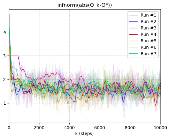
Figure 1: Showing decreasing error between ${\bm{Q}}_{k}$ and ${\bm{Q}}^{*}$ in a random MDP. Seven runs for the same MDP are conducted. Moving averages are highlighted as vivid line.

4.2 Performance on Benchmark Environments

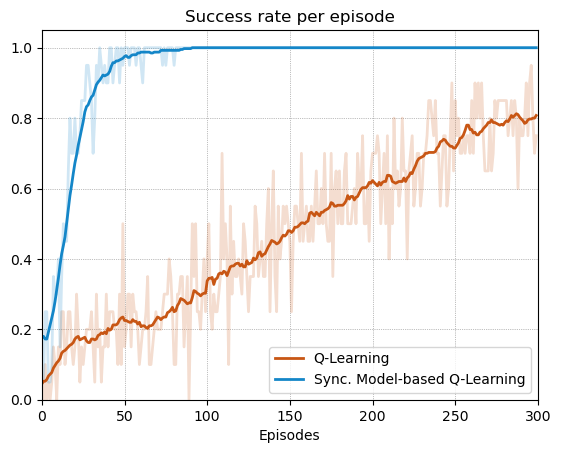
(a) Taxi, $\alpha=0.1$

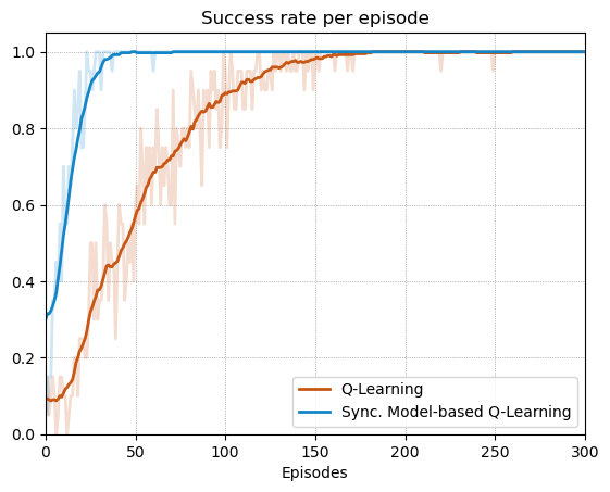
(b) Taxi, $\alpha=0.5$

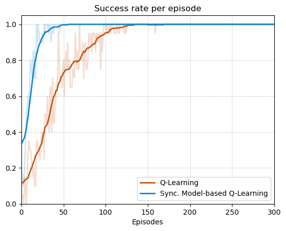
(c) Taxi, $\alpha=0.9$

$\alpha$	Q	SyncMBQ
0.1	0.95$\pm$1.20	98.30$\pm$4.83
0.5	45.35$\pm$5.99	98.75$\pm$3.24
0.9	61.00$\pm$3.95	88.25$\pm$9.80

(d) Taxi, Success rate (%) under greedy policy after training

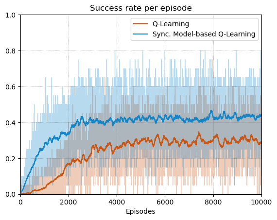
(e) FrozenLake, $\alpha=0.1$

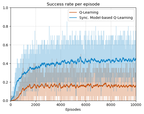
(f) FrozenLake, $\alpha=0.5$

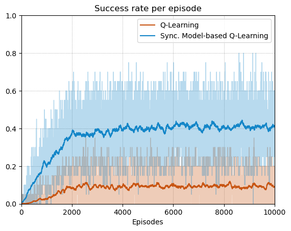
(g) FrozenLake, $\alpha=0.9$

$\alpha$	Q	SyncMBQ
$0.1$	47.15$\pm$19.00	71.25$\pm$4.44
$0.5$	19.15$\pm$15.22	71.10$\pm$4.85
$0.9$	18.35$\pm$15.01	54.20$\pm$16.66

(h) FrozenLake, Success rate (%) under greedy policy after training

Figure 2: Perfomance of the synchronous model-based $Q$-learning. Taxi (top row) and FrozenLake (bottom row). For graphs, moving averages are highlighted as vivid line with a window size of 20 episodes for Taxi and 100 for FrozenLake. For tables, the mean and standard deviation averaged over 20 runs are shown.

To evaluate the proposed SyncMBQ, we choose two environments from Gymnasium [Towers et al., 2023]: Taxi-v3 and FrozenLake8x8-v1. Experiments were conducted using constant step-size of $\alpha\in\{0.1,0.5,0.9\}$ and the results are averaged over 20 runs for each algorithm.

Taxi is a deterministic environment with $|{\mathcal{S}}|=500$ and $|{\mathcal{A}}|=6$. Each episode starts at random one of 300 possible starting states. Reward of $-1$ is given for each step, unless for a wrong pick-drop ($-10$) or for a successful drop ($+20$). An episode terminates after the drop action. FrozenLake is a stochastic environment with $|{\mathcal{S}}|=64$ and $|{\mathcal{A}}|=4$. The agent will move in intended direction with probability of $1/3$ else will move in either perpendicular direction with equal probability of $1/3$ in both directions. All episodes start at the top left starting point. The only reward of $1$ is given when the agent reaches the goal. An episode terminates when the agent fells into a hole or reaches the goal.

We see from Figure 2 that SyncMBQ performs better than the original $Q$-learning, especially in FrozenLake which is an stochastic environment. The left three columns show the average success rate while training. In Taxi shown at top row, SyncMBQ achieves full success on its early stage, while $Q$-learning gradually converges to the optimal policy. Similarly in FrozenLake at bottom row, the success rate of SyncMBQ is always higher then the standard $Q$-learning. We can get another advantage with SyncMBQ. While the performance of $Q$-learning depends a lot on learning rate $\alpha$, SyncMBQ shows stable outperformance. The rightmost column is about the success rate of greedy policy, since $\epsilon$-greedy behavior policy is used until the end of the training. This quantitative results again proves the superiority of SyncMBQ.

5 Conclusion

In this paper, we have studied the non-asymptotic behavior and empirical performance of SyncMBQ, which is direct extension of $Q$-learning to the model-based setting. We have considered online learning setting and relaxed sampling model which is weaker assumption than the generative model assumption. Furthermore, we proved that SyncMBQ can achieve the optimal sample complexity of $Q$-learning with general step-size. Moreover, we developed a new switched system model for $Q$-learning, and experimentally verified the superiority of SyncMBQ over $Q$-learning. Future studies include considering the setting where we collect samples following a single trajectory and dealing with the exploration-exploitation dilemma.

Supplementary Material

Appendix A Notations

${\mathbb{N}}$ : set of natural numbers; $\mathbb{R}^{n},\;n\in{\mathbb{N}}$ : set of real-valued $n$-dimensional vectors; $\mathbb{R}^{n\times m},\;n.m\in{\mathbb{N}}$ : set of real-valued $n\times m$-dimensional matrices; $[{\bm{v}}]_{i}$ for ${\bm{v}}\in\mathbb{R}^{n}$ and $1\leq i\leq n$: $i$-th element of ${\bm{v}}$; $[{\bm{A}}]_{i,j}$ for ${\bm{A}}\in\mathbb{R}^{n\times m},\;1\leq i\leq n,\;1\leq j\leq m$: $i$-th row and $j$-th column element of ${\bm{A}}$; $\otimes$ : Kronecker product; $\lceil a\rceil$ for $a\in\mathbb{R}$ : the smallest integer greater than or equal to $a\in\mathbb{R}$; $\lfloor a\rfloor$ for $a\in\mathbb{R}$ : the greatest integer less than or equal to $a\in\mathbb{R}$.

Appendix B Technical lemmas

B.1 Concentration inequalities

Lemma B.1 (Theorem B.6 in Shalev-Shwartz and Ben-David [2014]).

Let $X_{1},\dots,X_{n}$ be independent random variables such that $\mathbb{E}[X_{i}]=\mu$ and $a\leq X_{i}\leq b$ for every $i\in{\mathbb{N}}$. Then for any ${\epsilon}>0$, we have

$${\mathbb{P}}\left[\left|\frac{1}{n}\sum_{i=1}^{n}(X_{i}-\mu)\right|\geq{\epsilon}\right]\leq 2\exp(-2n{\epsilon}^{2}/(b-a)^{2}).$$

Lemma B.2.

For $s\in{\mathcal{S}},a\in{\mathcal{A}},k\in{\mathbb{N}}$, suppose that an event $\Omega$ depends on $s,a,k,{\epsilon}$, and state-action trajectory $\{(s_{k},a_{k},s_{k}^{\prime})\}_{k=1}^{\infty}$. Moreover, assume that for some positive constant $A,B$, the following holds:

$${\mathbb{P}}\left[\Omega(s,a,k,{\epsilon})\middle|N^{s,a}_{k}=t\right]\leq A\exp(-tB{\epsilon}^{2}),$$ (13)

for $1\leq t\leq k$, and $N^{s,a}_{k}$ denotes number of visits to state-action pair $(s,a)\in{\mathcal{S}}\times{\mathcal{A}}$. Then, we have

$${\mathbb{P}}\left[\Omega(s,a,k,{\epsilon})\right]\leq A\exp(-kd(s,a)B{\epsilon}^{2}/2)+\exp(-kd(s,a)),$$

for ${\epsilon}^{2}\in[0,1.59/B]$.

Proof B.3.

The law of total probability yields

$${\mathbb{P}}\left[\Omega(s,a,k,{\epsilon})\cap\{N^{s,a}_{k}\geq 1\}\right]= \sum^{k}_{t=1}{\mathbb{P}}\left[\Omega(s,a,k,{\epsilon})\middle|N^{sa}_{k}=t\right]{\mathbb{P}}[N^{s,a}_{k}=t]$$

$$\leq A\sum^{k}_{t=1}\exp(-tB{\epsilon}^{2})\binom{k}{t}d(s,a)^{t}(1-d(s,a))^{k-t}$$

$$= \sum^{k}_{t=1}A(d(s,a)\binom{k}{t}\exp(-B{\epsilon}^{2}))^{t}(1-d(s,a))^{k-t}$$

$$\leq A(1-d(s,a)+d(s,a)\exp(-B{\epsilon}^{2}))^{k}$$

$$\leq A\left(1-d(s,a)\frac{B{\epsilon}^{2}}{2}\right)^{k}$$

$$\leq A\exp(-kd(s,a)B{\epsilon}^{2}/2),$$ (14)

where the first inequality follows from the assumption, the second inequality follows from the binomial theorem, and the last inequality follows from $\exp(-x)\leq 1-\frac{x}{2}$ for $x\in[0,1.59]$. Next, it follows that

$${\mathbb{P}}\left[\Omega(s,a,k,{\epsilon})\right]= {\mathbb{P}}\left[\Omega(s,a,k,{\epsilon})\cap\{N^{sa}_{k}\geq 1\}\right]+{\mathbb{P}}\left[\Omega(s,a,k,{\epsilon})\cap\{N^{s,a}_{k}=0\right]$$

$$\leq A\exp(-kd(s,a)B{\epsilon}^{2}/2)+{\mathbb{P}}[N^{s,a}_{k}=0]$$

$$\leq A\exp(-kd(s,a)B{\epsilon}^{2}/2)+(1-d(s,a))^{k}$$

$$\leq A\exp(-kd(s,a)B{\epsilon}^{2}/2)+\exp(-kd(s,a)),$$

where the first inequality follows from (14), the second inequality follows from the fact that ${\mathbb{P}}[(s_{t},a_{t})=(s,a)]=d(s,a)$ for $1\leq t\leq k$, and the last inequality follows from the relation $1-x\leq\exp(-x)$ for $x\geq 0$.

B.2 Spectral properties

Lemma B.4.

For $k\in{\mathbb{N}}$, we have $\left\|{\bm{Q}}_{k}\right\|_{\infty}\leq\frac{1}{1-\gamma}$. Moreover, $\left\|{\bm{Q}}^{*}\right\|_{\infty}\leq\frac{1}{1-\gamma}$.

Proof B.5.

Suppose that the statement holds for some $k\in{\mathbb{N}}$, i.e., $\left\|{\bm{Q}}_{k}\right\|_{\infty}\leq\frac{1}{1-\gamma}$. Then, we have

$$\left\|{\bm{Q}}_{k+1}\right\|_{\infty}\leq (1-\alpha)\left\|{\bm{Q}}_{k}\right\|_{\infty}+\alpha(1+\gamma\left\|{\bm{Q}}_{k}\right\|_{\infty})$$

$$\leq \frac{1}{1-\gamma}-\alpha\frac{1}{1-\gamma}+\alpha+\alpha\frac{\gamma}{1-\gamma}$$

$$\leq \frac{1}{1-\gamma}.$$

The proof is completed by the induction argument. Moreover, since ${\bm{Q}}^{*}(s,a)=\mathbb{E}\left[\sum_{k=1}^{\infty}\gamma^{k}r_{k}\mid s,a,\pi^{*}\right]$, and $|r_{k}|\leq 1$, we have $|{\bm{Q}}^{*}(s,a)|\leq\frac{1}{1-\gamma}$.

Lemma B.6.

For $k\in{\mathbb{N}}$, we have $\left\|{\bm{w}}_{k}\right\|_{\infty}\leq\frac{2}{1-\gamma}$.

Proof B.7.

Applying triangle inequality to ${\bm{w}}_{k}$ in (8) yields

$$\left\|{\bm{w}}_{k}\right\|_{\infty}\leq \left\|\hat{{\bm{R}}}_{k}-{\bm{R}}\right\|_{\infty}+\gamma\left\|{\bm{\Pi}}^{{\bm{Q}}^{*}}{\bm{Q}}^{*}\right\|_{\infty}\left\|\hat{{\bm{P}}}_{k}-{\bm{P}}\right\|_{\infty}$$

$$\leq \left\|\hat{{\bm{R}}}_{k}-{\bm{R}}\right\|_{\infty}+\frac{\gamma}{1-\gamma}\left\|\hat{{\bm{P}}}_{k}-{\bm{P}}\right\|_{\infty}$$

$$\leq 2+\frac{2\gamma}{1-\gamma}$$

$$= \frac{2}{1-\gamma},$$

where the second inequality follows from Lemma B.4 in the Appendix Section B.2.

Appendix C Omitted Proofs

C.1 Proof of Lemma 3.2

Proof C.1.

Applying the union bound, we have

$${\mathbb{P}}\left[\{N^{s,a}_{m}\geq 1,\;\forall(s,a)\in{\mathcal{S}}\times{\mathcal{A}}\}^{c}\right]\leq \sum_{s,a\in{\mathcal{S}}\times{\mathcal{A}}}{\mathbb{P}}\left[N^{s,a}_{m}=0\right]$$

$$\leq |{\mathcal{S}}||{\mathcal{A}}|(1-d_{\min})^{m}$$

$$\leq |{\mathcal{S}}||{\mathcal{A}}|\exp(-md_{\min})$$

$$\leq \frac{\delta}{2},$$

where the second inequality follows from the fact that the probability of observing $(s,a)$ is $d(s,a)$ while probability of observing different state-action pair is $1-d(s,a)$, the third inequality holds from the fact that $1-x\leq\exp(-x)$, and the last inequality follows from choice of $m$.

C.2 Proof of Lemma 3.4

Proof C.2.

Note that under event ${\mathcal{E}}$ defined in (6), we have $\sum_{j=1}^{|{\mathcal{S}}|}[\hat{{\bm{P}}}_{k}]_{i,j}=1$ for $1\leq i\leq|{\mathcal{S}}||{\mathcal{A}}|$. Therefore, we have $\sum^{|{\mathcal{S}}||{\mathcal{A}}|}_{j=1}[\hat{{\bm{P}}}{\bm{\Pi}}^{{\bm{Q}}}]_{i,j}=\sum^{|{\mathcal{S}}||{\mathcal{A}}|}_{j=1}\sum_{h=1}^{|{\mathcal{S}}|}[\hat{{\bm{P}}}_{k}]_{i,h}[{\bm{\Pi}}^{{\bm{Q}}}]_{h,j}=\sum_{h=1}^{|{\mathcal{S}}|}[\hat{{\bm{P}}}_{k}]_{i,h}\sum_{j=1}^{|{\mathcal{S}}||{\mathcal{A}}|}[{\bm{\Pi}}^{{\bm{Q}}}]_{h,j}=1$.

Hence, we get

$$\left\|(1-\alpha){\bm{I}}+\gamma\alpha\hat{{\bm{P}}}_{k}{\bm{\Pi}}^{{\bm{Q}}}\right\|_{\infty}\leq 1-\alpha+\gamma\alpha\max_{1\leq i\leq|{\mathcal{S}}||{\mathcal{A}}|}\left(\sum_{j=1}^{|{\mathcal{S}}||{\mathcal{A}}|}[\hat{{\bm{P}}}_{k}{\bm{\Pi}}^{{\bm{Q}}}]_{i,j}\right)$$

$$= 1-(1-\gamma)\alpha.$$

This completes the proof.

C.3 Proof of Lemma 3.5

Proof C.3.

We will first check the condition in (13) to apply Lemma B.2. From Lemma B.4, we have $\left\|\hat{{\bm{P}}}_{k}{\bm{\Pi}}^{{\bm{Q}}^{*}}{\bm{Q}}^{*}\right\|_{\infty}\leq\frac{1}{1-\gamma}$. Moreover, noting that $\mathbb{E}\left[[\hat{{\bm{P}}}_{k}{\bm{\Pi}}^{{\bm{Q}}^{*}}{\bm{Q}}^{*}]_{s,a}\right]=[{\bm{P}}{\bm{\Pi}}^{{\bm{Q}}^{*}}{\bm{Q}}^{*}]_{s,a}$, from Lemma B.1, we get, for $1\leq t\leq k$,

$${\mathbb{P}}\left[\left|[\hat{{\bm{P}}}_{k}{\bm{\Pi}}^{{\bm{Q}}^{*}}{\bm{Q}}^{*}]_{s,a}-[{\bm{P}}{\bm{\Pi}}^{{\bm{Q}}^{*}}{\bm{Q}}^{*}]_{s,a}\right|\geq{\epsilon}\middle|N^{s,a}_{k}=t\right]\leq 2\exp(-t{\epsilon}^{2}(1-\gamma)^{2}/2).$$

Hence, we can now apply Lemma B.2, which yields

$${\mathbb{P}}\left[\left|[\hat{{\bm{P}}}_{k}{\bm{\Pi}}^{{\bm{Q}}^{*}}{\bm{Q}}^{*}]_{s,a}-[{\bm{P}}{\bm{\Pi}}^{{\bm{Q}}^{*}}{\bm{Q}}^{*}]_{s,a}\right|\geq{\epsilon}\right]\leq 2\exp(-kd(s,a)(1-\gamma)^{2}{\epsilon}^{2}/4)+\exp(-kd(s,a))$$

$$\leq 3\exp(-kd(s,a)(1-\gamma)^{2}{\epsilon}^{2}/4).$$ (15)

The union bound leads to

$${\mathbb{P}}\left[\left\|\hat{{\bm{P}}}_{k}{\bm{\Pi}}^{{\bm{Q}}^{*}}{\bm{Q}}^{*}-{\bm{P}}{\bm{\Pi}}^{{\bm{Q}}^{*}}{\bm{Q}}^{*}\right\|_{\infty}\geq{\epsilon}\right]= {\mathbb{P}}\left[\max_{s,a\in{\mathcal{S}}\times{\mathcal{A}}}\left|[\hat{{\bm{P}}}_{k}{\bm{\Pi}}^{{\bm{Q}}^{*}}{\bm{Q}}^{*}-{\bm{P}}{\bm{\Pi}}^{{\bm{Q}}^{*}}{\bm{Q}}^{*}]_{s,a}\right|\geq{\epsilon}\right]$$

$$\leq \sum_{s,a\in{\mathcal{S}}\times{\mathcal{A}}}{\mathbb{P}}\left[\left|[\hat{{\bm{P}}}_{k}{\bm{\Pi}}^{{\bm{Q}}^{*}}{\bm{Q}}^{*}-{\bm{P}}{\bm{\Pi}}^{{\bm{Q}}^{*}}{\bm{Q}}^{*}]_{s,a}\right|\geq{\epsilon}\right]$$

$$\leq 3|{\mathcal{S}}||{\mathcal{A}}|\exp(-kd_{\min}(1-\gamma)^{2}{\epsilon}^{2}/4),$$

where the first inequality follows from $\left\{\max_{(s,a)\in{\mathcal{S}}\times{\mathcal{A}}}\left|[\hat{{\bm{P}}}_{k}{\bm{\Pi}}^{{\bm{Q}}^{*}}{\bm{Q}}^{*}-{\bm{P}}{\bm{\Pi}}^{{\bm{Q}}^{*}}{\bm{Q}}^{*}]_{s,a}\right\|\geq{\epsilon}\right\}\subset\cup_{(s,a)\in{\mathcal{S}}\times{\mathcal{A}}}\left\{\left|[\hat{{\bm{P}}}_{k}{\bm{\Pi}}^{{\bm{Q}}^{*}}{\bm{Q}}^{*}-{\bm{P}}{\bm{\Pi}}^{{\bm{Q}}^{*}}{\bm{Q}}^{*}]_{s,a}\right|\geq{\epsilon}\right\}$, and the last inequality follows from (15). Furthermore, we can derive the concentration bound for $\hat{{\bm{R}}}_{k}$ in the same manner. From Lemma B.1, we have

$${\mathbb{P}}\left[\left|\hat{r}^{s,a}_{k}-{\bm{R}}^{s,a}_{k}\right|\geq{\epsilon}\middle|N^{s,a}_{k}=t\right]\leq 2\exp(-t{\epsilon}^{2}/2).$$

Therefore, from Lemma B.2, one gets

$${\mathbb{P}}\left[\left|\hat{r}^{s,a}_{k}-{\bm{R}}^{s,a}_{k}\right|\geq{\epsilon}\right]\leq 2\exp(-kd(s,a){\epsilon}^{2}/4)+\exp(-kd(s,a))\leq 3\exp(-kd(s,a){\epsilon}^{2}/4).$$

Applying the union bound leads to

$${\mathbb{P}}\left[\left\|\hat{{\bm{R}}}_{k}-{\bm{R}}\right\|_{\infty}\geq{\epsilon}\right]= {\mathbb{P}}\left[\max_{s,a\in{\mathcal{S}}\times{\mathcal{A}}}|\hat{r}^{s,a}_{k}-{\bm{R}}^{s,a}|\geq{\epsilon}\right]$$

$$\leq \sum_{s,a\in{\mathcal{S}}\times{\mathcal{A}}}{\mathbb{P}}\left[|\hat{r}^{s,a}_{k}-{\bm{R}}^{s,a}|\geq{\epsilon}\right]$$

$$\leq 3|{\mathcal{S}}||{\mathcal{A}}|\exp(-kd_{\min}{\epsilon}^{2}/4).$$

This completes the proof.

C.4 Proof of Lemma 3.6

Proof C.4.

Applying triangle inequality to the definition of ${\bm{w}}_{k}$ in (8) leads to

$$\left\|{\bm{w}}_{k}\right\|_{\infty}\leq\left\|\hat{{\bm{R}}}_{k}-{\bm{R}}\right\|_{\infty}+\gamma\left\|\hat{{\bm{P}}}_{k}{\bm{\Pi}}^{{\bm{Q}}^{*}}{\bm{Q}}^{*}-{\bm{P}}{\bm{\Pi}}^{{\bm{Q}}^{*}}{\bm{Q}}^{*}\right\|_{\infty}.$$

Therefore, the following holds:

$${\mathbb{P}}\left[\left\|{\bm{w}}_{k}\right\|_{\infty}<{\epsilon}\right]\geq{\mathbb{P}}\left[\left\{\left\|\hat{{\bm{R}}}_{k}-{\bm{R}}\right\|_{\infty}<\frac{{\epsilon}}{2}\right\}\cap\left\{\left\|\hat{{\bm{P}}}_{k}{\bm{\Pi}}^{{\bm{Q}}^{*}}{\bm{Q}}^{*}-{\bm{P}}{\bm{\Pi}}^{{\bm{Q}}^{*}}{\bm{Q}}^{*}\right\|_{\infty}<\frac{{\epsilon}}{2\gamma}\right\}\right].$$

Considering the complement of the event $\{\left\|\tilde{{\bm{w}}}_{k}\right\|_{\infty}<{\epsilon}\}^{c}=\{\left\|\tilde{{\bm{w}}}_{k}\right\|_{\infty}\geq{\epsilon}\}$,

$${\mathbb{P}}\left[\left\|{\bm{w}}_{k}\right\|_{\infty}\geq{\epsilon}\right]\leq {\mathbb{P}}\left[\left\{\left\|\hat{{\bm{R}}}_{k}-{\bm{R}}\right\|_{\infty}\geq\frac{{\epsilon}}{2}\right\}\cup\left\{\left\|\hat{{\bm{P}}}_{k}{\bm{\Pi}}^{{\bm{Q}}^{*}}{\bm{Q}}^{*}-{\bm{P}}{\bm{\Pi}}^{{\bm{Q}}^{*}}{\bm{Q}}^{*}\right\|_{\infty}\geq\frac{{\epsilon}}{2\gamma}\right\}\right]$$

$$\leq {\mathbb{P}}\left[\left\|\hat{{\bm{R}}}_{k}-{\bm{R}}\right\|_{\infty}\geq\frac{{\epsilon}}{2}\right]+{\mathbb{P}}\left[\left\|\hat{{\bm{P}}}_{k}{\bm{\Pi}}^{{\bm{Q}}^{*}}{\bm{Q}}^{*}-{\bm{P}}{\bm{\Pi}}^{{\bm{Q}}^{*}}{\bm{Q}}^{*}\right\|_{\infty}\geq\frac{{\epsilon}}{2\gamma}\right]$$

$$\leq 3|{\mathcal{S}}||{\mathcal{A}}|\exp(-kd_{\min}{\epsilon}^{2}/16)+3|{\mathcal{S}}||{\mathcal{A}}|\exp(-kd_{\min}(1-\gamma)^{2}{\epsilon}^{2}/(16\gamma^{2}))$$

$$\leq 6|{\mathcal{S}}||{\mathcal{A}}|\exp(-kd_{\min}(1-\gamma)^{2}{\epsilon}^{2}/16),$$

where the second inequality follows from union bound and the third inequality follows from Lemma 3.5.

C.5 Proof of Theorem 3.7

Proof C.5.

Suppose the following event holds, for $k\geq m$:

$$W_{k}:=\left\{\left\|{\bm{w}}_{i}\right\|_{\infty}\leq{\epsilon}^{\prime},\;\forall\left\lceil\frac{k-m}{2}\right\rceil+m\leq i\leq k\right\},$$

The choice of positive constant ${\epsilon}^{\prime}$ will be deferred. Recursively expanding (12), we have

$${\bm{x}}_{k+1}=\prod_{i=m}^{k}{\bm{A}}^{{\bm{y}}_{i}}_{i}{\bm{x}}_{m}+\alpha\sum_{i=m}^{k-1}\prod_{j=i+1}^{k}{\bm{A}}^{{\bm{y}}_{j}}_{j}{\bm{w}}_{i}+\alpha{\bm{w}}_{k}.$$

Under the event ${\mathcal{E}}$ in (6), we have $\left\|{\bm{A}}^{{\bm{y}}_{k}}_{k}\right\|_{\infty}\leq 1-(1-\gamma)\alpha$. Taking infinity norm on the above equation, and applying triangle inequality, we get,

$$\left\|{\bm{x}}_{k+1}\right\|_{\infty}\leq \left\|\prod^{k}_{i=m}{\bm{A}}^{{\bm{y}}_{i}}_{i}{\bm{x}}_{m}\right\|_{\infty}+\alpha\sum^{k-1}_{i=m}\prod_{j=i+1}^{k}\left\|{\bm{A}}^{{\bm{y}}_{j}}_{j}\right\|_{\infty}\left\|{\bm{w}}_{i}\right\|_{\infty}+\alpha\left\|{\bm{w}}_{k}\right\|_{\infty}$$

$$\leq (1-(1-\gamma)\alpha)^{k-m+1}\left\|{\bm{x}}_{m}\right\|_{\infty}+\alpha\underbrace{\sum^{k-1}_{i=m}(1-(1-\gamma)\alpha)^{k-i}\left\|{\bm{w}}_{i}\right\|_{\infty}}_{(\star)}+\alpha\left\|{\bm{w}}_{k}\right\|_{\infty}$$

$$\leq (1-(1-\gamma)\alpha)^{k-m+1}\left\|{\bm{x}}_{m}\right\|_{\infty}+\alpha\sum^{m+\lfloor\frac{k-m}{2}\rfloor}_{i=m}(1-(1-\gamma)\alpha)^{k-i}\left\|{\bm{w}}_{i}\right\|_{\infty}$$

$$+\alpha\sum^{k-1}_{i=m+\lceil\frac{k-m}{2}\rceil}(1-(1-\gamma)\alpha)^{k-i}\left\|{\bm{w}}_{i}\right\|_{\infty}+\alpha\left\|{\bm{w}}_{k}\right\|_{\infty}$$

$$\leq \underbrace{\frac{2}{1-\gamma}\exp(-(1-\gamma)\alpha(k-m+1))}_{E_{1}}+\underbrace{\frac{2}{(1-\gamma)^{2}}(1-(1-\gamma)\alpha)^{k-m-\lceil\frac{k-m}{2}\rceil}}_{E_{2}}+\underbrace{\frac{2}{1-\gamma}{\epsilon}^{\prime}}_{E_{3}},$$

where the third inequality follows from decomposition of $(\star)$ and the last inequality follows from Lemma B.6 and the definition of event $W_{k}$.

Our aim is to bound the above inequality with ${\epsilon}$. One sufficient condition to achieve the bound is to bound each $E_{1},E_{2}$, and $E_{3}$ with ${\epsilon}/3$. First, to bound $E_{1}$, we need $\exp(-(1-\gamma)\alpha(k-m+1))\leq\frac{{\epsilon}(1-\gamma)}{3}$, which is satisfied when

$$k\geq m+\frac{1}{\alpha(1-\gamma)}\ln\frac{6}{{\epsilon}(1-\gamma)}.$$ (16)

Next, to bound $E_{2}$, we require,

$$\frac{2}{(1-\gamma)^{2}}(1-(1-\gamma)\alpha)^{k-m-\lfloor\frac{k-m}{2}\rfloor}\leq\frac{2}{(1-\gamma)^{2}}(1-(1-\gamma)\alpha)^{\frac{k-m}{2}}\leq\frac{2}{(1-\gamma)^{2}}\exp\left(-\frac{(1-\gamma)\alpha}{2}(k-m)\right)\leq\frac{{\epsilon}}{3},$$

which is satisfied if

$$\frac{k-m}{2}\geq\frac{2}{(1-\gamma)\alpha}\ln\left(\frac{6}{{\epsilon}(1-\gamma)^{2}}\right)\iff k\geq\frac{4}{(1-\gamma)\alpha}\ln\left(\frac{6}{{\epsilon}(1-\gamma)^{2}}\right)+m.$$ (17)

To bound $E_{3}$ with $\frac{{\epsilon}}{3}$, we require, ${\epsilon}^{\prime}\leq\frac{1-\gamma}{6}{\epsilon}$.

Therefore, it is enough to find $k$ such that the event $W_{k}$ under ${\mathcal{E}}$ with ${\epsilon}^{\prime}=\frac{1-\gamma}{6}{\epsilon}$ to hold with probability at least $1-\frac{\delta}{2}$ from the following relation:

$${\mathbb{P}}\left[\left\|{\bm{Q}}_{k}-{\bm{Q}}^{*}\right\|_{\infty}\leq{\epsilon}\middle|{\mathcal{E}}\right]\geq{\mathbb{P}}\left[W_{k}\middle|{\mathcal{E}}\right]\geq 1-\frac{\delta}{2}.$$ (18)

Taking the the complement of the event $W_{k}$ yields

$${\mathbb{P}}\left[W^{c}_{k}\middle|{\mathcal{E}}\right]= {\mathbb{P}}\left[\cup^{k}_{i=m+\lceil\frac{k-m}{2}\rceil}\left\{\left\|{\bm{w}}_{i}\right\|_{\infty}\geq\frac{1-\gamma}{6}{\epsilon}\right\}\middle|{\mathcal{E}}\right]$$

$$= \frac{1}{{\mathbb{P}}[{\mathcal{E}}]}{\mathbb{P}}\left[\cup^{k}_{i=m+\lceil\frac{k-m}{2}\rceil}\left\{\left\|{\bm{w}}_{i}\right\|_{\infty}\geq\frac{1-\gamma}{6}{\epsilon}\right\}\cap{\mathcal{E}}\right]$$

$$\leq \frac{{\mathbb{P}}\left[\cup^{k}_{i=m+\lceil\frac{k-m}{2}\rceil}\left\{\left\|{\bm{w}}_{i}\right\|_{\infty}\geq\frac{1-\gamma}{6}{\epsilon}\right\}\right]}{{\mathbb{P}}[{\mathcal{E}}]}$$

$$\leq \frac{1}{{\mathbb{P}}[{\mathcal{E}}]}\sum^{k}_{i=m+\lceil\frac{k-m}{2}\rceil}{\mathbb{P}}\left[\left\|{\bm{w}}_{i}\right\|_{\infty}\geq\frac{1-\gamma}{6}{\epsilon}\right]$$

$$\leq \frac{6|{\mathcal{S}}||{\mathcal{A}}|}{1-\delta/2}\left(k-m+1-\left\lceil\frac{k-m}{2}\right\rceil\right)\exp\left(-\left(m+\left\lceil\frac{k-m}{2}\right\rceil\right)d_{\min}(1-\gamma)^{4}{\epsilon}^{2}/576\right),$$

where the second equality follows from the law of conditional probability. The last inequality follows from Lemma 3.2 and Lemma 3.6. For ${\mathbb{P}}[W^{c}_{k}|{\mathcal{E}}]\leq\frac{\delta}{2}$ to hold, the following condition is sufficient:

$$k\geq m+2+\frac{1152}{{\epsilon}^{2}(1-\gamma)^{4}d_{\min}}\ln\left(\frac{12k|{\mathcal{S}}||{\mathcal{A}}|}{\delta(1-\delta/2)}\right).$$

Noting that $\delta(1-\delta/2)\geq\delta/2$, the following number of samples is sufficient:

$$k\geq m+2+\frac{1152}{{\epsilon}^{2}(1-\gamma)^{4}d_{\min}}\ln\left(\frac{24k|{\mathcal{S}}|{\mathcal{A}}|}{\delta}\right).$$ (19)

Letting $k$ be the minimum value satisfying the inequalities in (16), (17) and (19), we have $\left\|{\bm{Q}}_{k}-{\bm{Q}}^{*}\right\|_{\infty}\leq{\epsilon}$ with probability at least $1-\frac{\delta}{2}$ under event ${\mathcal{E}}$.

The law of total probability yields

$${\mathbb{P}}\left[\left\|{\bm{Q}}_{k}-{\bm{Q}}^{*}\right\|_{\infty}\geq{\epsilon}\right]= {\mathbb{P}}\left[\left\{\left\|{\bm{Q}}_{k}-{\bm{Q}}^{*}\right\|_{\infty}\geq{\epsilon}\right\}\middle|{\mathcal{E}}\right]{\mathbb{P}}[{\mathcal{E}}]+{\mathbb{P}}\left[\left\{\left\|{\bm{Q}}_{k}-{\bm{Q}}^{*}\right\|_{\infty}\geq{\epsilon}\right\}\middle|{\mathcal{E}}^{c}\right]{\mathbb{P}}[{\mathcal{E}}^{c}]$$

$$\leq {\mathbb{P}}\left[\left\|{\bm{Q}}_{k}-{\bm{Q}}^{*}\right\|_{\infty}\geq{\epsilon}\middle|{\mathcal{E}}\right]+{\mathbb{P}}[{\mathcal{E}}^{c}]$$

$$\leq \frac{\delta}{2}+\frac{\delta}{2}$$

$$= \delta.$$

The second last inequality follows from (18) and Lemma 3.2.

Appendix D Upper and lower comparison system derivation

Lemma D.1.

For $k\in{\mathbb{N}}$, we have ${\bm{Q}}^{U}_{k}\geq{\bm{Q}}_{k}$,

Proof D.2.

The proof follows from induction on the hypothesis ${\bm{Q}}^{U}_{k}\geq{\bm{Q}}_{k}$. Suppose that the argument holds for some $k\in{\mathbb{N}}$. Then, letting $\tilde{{\bm{Q}}}^{U}_{k}={\bm{Q}}^{U}_{k}-{\bm{Q}}^{*}$, we have $\tilde{{\bm{Q}}}^{U}_{k}\geq\tilde{{\bm{Q}}}_{k}$. Now, we show that the following argument holds for $\tilde{{\bm{Q}}}^{U}_{k+1}$:

$$\tilde{{\bm{Q}}}^{U}_{k+1}= {\bm{A}}^{{\bm{Q}}_{k}}_{k}\tilde{{\bm{Q}}}^{U}_{k}+\alpha{\bm{w}}_{k}$$

$$\geq {\bm{A}}^{{\bm{Q}}_{k}}_{k}\tilde{{\bm{Q}}}_{k}+\alpha\gamma\hat{{\bm{P}}}_{k}({\bm{\Pi}}^{{\bm{Q}}_{k}}-{\bm{\Pi}}^{{\bm{Q}}^{*}}){\bm{Q}}^{*}+\alpha{\bm{w}}_{k}$$

$$= \tilde{{\bm{Q}}}_{k+1},$$

where the first inequality follows from the fact that ${\bm{A}}^{{\bm{Q}}_{k}}_{k}$ is a positive matrix, i.e., the elements of ${\bm{A}}^{{\bm{Q}}_{k}}_{k}$ are all non-negative, and the fact that ${\bm{\Pi}}^{{\bm{Q}}^{*}}{\bm{Q}}^{*}\geq{\bm{\Pi}}^{{\bm{Q}}_{k}}{\bm{Q}}^{*}$. The proof is completed by the induction argument.

Lemma D.3.

For $k\in{\mathbb{N}}$, we have ${\bm{Q}}^{L}_{k}\leq{\bm{Q}}_{k}$.

Proof D.4.

Let $\tilde{{\bm{Q}}}^{L}_{k}:={\bm{Q}}^{L}_{k}-{\bm{Q}}^{*}$. Suppose the argument holds for some $k\in{\mathbb{N}}$. Then, we have

$$\tilde{{\bm{Q}}}^{L}_{k+1}= {\bm{A}}^{{\bm{Q}}^{*}}_{k}\tilde{{\bm{Q}}}^{L}_{k}+\alpha{\bm{w}}_{k}$$

$$= (1-\alpha)\tilde{{\bm{Q}}}^{L}_{k}+\alpha\gamma\hat{{\bm{P}}}_{k}{\bm{\Pi}}^{{\bm{Q}}^{*}}\tilde{{\bm{Q}}}^{L}_{k}+\alpha{\bm{w}}_{k}$$

$$\leq (1-\alpha)\tilde{{\bm{Q}}}_{k}+\alpha\gamma\hat{{\bm{P}}}_{k}{\bm{\Pi}}^{{\bm{Q}}^{*}}{\bm{Q}}^{L}_{k}-\alpha\gamma\hat{{\bm{P}}}_{k}{\bm{\Pi}}^{{\bm{Q}}^{*}}{\bm{Q}}^{*}+\alpha{\bm{w}}_{k}$$

$$\leq (1-\alpha)\tilde{{\bm{Q}}}_{k}+\alpha\gamma\hat{{\bm{P}}}_{k}{\bm{\Pi}}^{{\bm{Q}}_{k}}{\bm{Q}}_{k}-\alpha\gamma\hat{{\bm{P}}}_{k}{\bm{\Pi}}^{{\bm{Q}}^{*}}{\bm{Q}}^{*}+\alpha{\bm{w}}_{k}$$

$$= ((1-\alpha){\bm{I}}+\gamma\hat{{\bm{P}}}_{k}{\bm{\Pi}}^{{\bm{Q}}_{k}})\tilde{{\bm{Q}}}_{k}+\alpha\gamma\hat{{\bm{P}}}_{k}{\bm{\Pi}}^{{\bm{Q}}_{k}}{\bm{Q}}^{*}-\alpha\gamma\hat{{\bm{P}}}_{k}{\bm{\Pi}}^{{\bm{Q}}^{*}}{\bm{Q}}^{*}+\alpha{\bm{w}}_{k}$$

$$= \tilde{{\bm{Q}}}_{k+1},$$

where the first inequality follows from the induction hypothesis, the second inequality follows from the relation ${\bm{\Pi}}^{{\bm{Q}}^{*}}{\bm{Q}}^{L}_{k}\leq{\bm{\Pi}}^{{\bm{Q}}^{L}_{k}}{\bm{Q}}^{L}_{k}\leq{\bm{\Pi}}^{{\bm{Q}}^{L}_{k}}{\bm{Q}}_{k}\leq{\bm{\Pi}}^{{\bm{Q}}_{k}}{\bm{Q}}_{k}$, and the last equality follows from (7). The proof is completed by the induction argument.

D.1 Proof of Lemma 3.3

Proof D.5.

The proof is readily completed using Lemma D.3 and D.1.

References

• Agarwal etย al. [2020] Alekh Agarwal, Sham Kakade, and Linย F Yang. Model-based reinforcement learning with a generative model is minimax optimal. In Conference on Learning Theory, pages 67โ€“83. PMLR, 2020.
• Azar etย al. [2012] Mohammadย Gheshlaghi Azar, Rรฉmi Munos, and Bert Kappen. On the sample complexity of reinforcement learning with a generative model. arXiv preprint arXiv:1206.6461, 2012.
• Bellman [1966] Richard Bellman. Dynamic programming. Science, 153(3731):34โ€“37, 1966.
• Brafman and Tennenholtz [2002] Ronenย I Brafman and Moshe Tennenholtz. R-max-a general polynomial time algorithm for near-optimal reinforcement learning. Journal of Machine Learning Research, 3(Oct):213โ€“231, 2002.
• Chen etย al. [2019] Zaiwei Chen, Sheng Zhang, Thinhย T Doan, Sivaย Theja Maguluri, and John-Paul Clarke. Performance of q-learning with linear function approximation: Stability and finite-time analysis. arXiv preprint arXiv:1905.11425, pageย 4, 2019.
• Chua etย al. [2018] Kurtland Chua, Roberto Calandra, Rowan McAllister, and Sergey Levine. Deep reinforcement learning in a handful of trials using probabilistic dynamics models. Advances in neural information processing systems, 31, 2018.
• Fawzi etย al. [2022] Alhussein Fawzi, Matej Balog, Aja Huang, Thomas Hubert, Bernardino Romera-Paredes, Mohammadamin Barekatain, Alexander Novikov, Franciscoย J Rย Ruiz, Julian Schrittwieser, Grzegorz Swirszcz, etย al. Discovering faster matrix multiplication algorithms with reinforcement learning. Nature, 610(7930):47โ€“53, 2022.
• Gheshlaghiย Azar etย al. [2013] Mohammad Gheshlaghiย Azar, Rรฉmi Munos, and Hilbertย J Kappen. Minimax pac bounds on the sample complexity of reinforcement learning with a generative model. Machine learning, 91:325โ€“349, 2013.
• Johnson and Zhang [2013] Rie Johnson and Tong Zhang. Accelerating stochastic gradient descent using predictive variance reduction. Advances in neural information processing systems, 26, 2013.
• Kalathil etย al. [2021] Dileep Kalathil, Vivekย S Borkar, and Rahul Jain. Empirical q-value iteration. Stochastic Systems, 11(1):1โ€“18, 2021.
• Kearns and Singh [1998] Michael Kearns and Satinder Singh. Finite-sample convergence rates for q-learning and indirect algorithms. Advances in neural information processing systems, 11, 1998.
• Kearns and Singh [2002] Michael Kearns and Satinder Singh. Near-optimal reinforcement learning in polynomial time. Machine learning, 49:209โ€“232, 2002.
• Kidambi etย al. [2020] Rahul Kidambi, Aravind Rajeswaran, Praneeth Netrapalli, and Thorsten Joachims. Morel: Model-based offline reinforcement learning. Advances in neural information processing systems, 33:21810โ€“21823, 2020.
• Lattimore and Hutter [2014] Tor Lattimore and Marcus Hutter. Near-optimal pac bounds for discounted mdps. Theoretical Computer Science, 558:125โ€“143, 2014.
• Lee and He [2019] Donghwan Lee and Niao He. A unified switching system perspective and ode analysis of q-learning algorithms. arXiv preprint arXiv:1912.02270, 2019.
• Lee [2022] Donghwna Lee. Finite-time analysis of constant step-size q-learning: Switching system approach revisited. arXiv preprint arXiv:2205.05455, 2022.
• Li etย al. [2020] Gen Li, Yuting Wei, Yuejie Chi, Yuantao Gu, and Yuxin Chen. Breaking the sample size barrier in model-based reinforcement learning with a generative model. Advances in neural information processing systems, 33:12861โ€“12872, 2020.
• Li etย al. [2023] Gen Li, Changxiao Cai, Yuxin Chen, Yuting Wei, and Yuejie Chi. Is q-learning minimax optimal? a tight sample complexity analysis. Operations Research, 2023.
• Liberzon [2005] Daniel Liberzon. Switched systems. In Handbook of networked and embedded control systems, pages 559โ€“574. Springer, 2005.
• Nagabandi etย al. [2018] Anusha Nagabandi, Gregory Kahn, Ronaldย S Fearing, and Sergey Levine. Neural network dynamics for model-based deep reinforcement learning with model-free fine-tuning. In 2018 IEEE international conference on robotics and automation (ICRA), pages 7559โ€“7566. IEEE, 2018.
• Qu and Wierman [2020] Guannan Qu and Adam Wierman. Finite-time analysis of asynchronous stochastic approximation and $q$-learning. In Conference on Learning Theory, pages 3185โ€“3205. PMLR, 2020.
• Shalev-Shwartz and Ben-David [2014] Shai Shalev-Shwartz and Shai Ben-David. Understanding machine learning: From theory to algorithms. Cambridge university press, 2014.
• Sidford etย al. [2018] Aaron Sidford, Mengdi Wang, Xian Wu, Lin Yang, and Yinyu Ye. Near-optimal time and sample complexities for solving markov decision processes with a generative model. Advances in Neural Information Processing Systems, 31, 2018.
• Silver etย al. [2017] David Silver, Julian Schrittwieser, Karen Simonyan, Ioannis Antonoglou, Aja Huang, Arthur Guez, Thomas Hubert, Lucas Baker, Matthew Lai, Adrian Bolton, etย al. Mastering the game of go without human knowledge. nature, 550(7676):354โ€“359, 2017.
• Strehl and Littman [2005] Alexanderย L Strehl and Michaelย L Littman. A theoretical analysis of model-based interval estimation. In Proceedings of the 22nd international conference on Machine learning, pages 856โ€“863, 2005.
• Strehl etย al. [2006] Alexanderย L Strehl, Lihong Li, Eric Wiewiora, John Langford, and Michaelย L Littman. Pac model-free reinforcement learning. In Proceedings of the 23rd international conference on Machine learning, pages 881โ€“888, 2006.
• Szita and Szepesvรกri [2010] Istvรกn Szita and Csaba Szepesvรกri. Model-based reinforcement learning with nearly tight exploration complexity bounds. In Proceedings of the 27th International Conference on Machine Learning (ICML-10), pages 1031โ€“1038, 2010.
• Towers etย al. [2023] Mark Towers, Jordanย K. Terry, Ariel Kwiatkowski, Johnย U. Balis, Gianlucaย de Cola, Tristan Deleu, Manuel Goulรฃo, Andreas Kallinteris, Arjun KG, Markus Krimmel, Rodrigo Perez-Vicente, Andrea Pierrรฉ, Sander Schulhoff, Junย Jet Tai, Andrew Tanย Jin Shen, and Omarย G. Younis. Gymnasium, March 2023. URL https://zenodo.org/record/8127025.
• Wainwright [2019] Martinย J Wainwright. Variance-reduced $q$-learning is minimax optimal. arXiv preprint arXiv:1906.04697, 2019.
• Watkins and Dayan [1992] Christopherย JCH Watkins and Peter Dayan. Q-learning. Machine learning, 8:279โ€“292, 1992.
• Wiering and Schmidhuber [1998] MAย Wiering and Jรผrgen Schmidhuber. Efficient model-based exploration. 1998.