Mitigation of systematic amplitude error in nonadiabatic holonomic operations

Abstract

Nonadiabatic holonomic operations are based on nonadiabatic non-Abelian geometric phases, hence possessing the inherent geometric features for robustness against control errors. However, nonadiabatic holonomic operations are still sensitive to the systematic amplitude error induced by imperfect control of pulse timing or laser intensity. In this work, we present a simple scheme of nonadiabatic holonomic operations in order to mitigate the said systematic amplitude error. This is achieved by introducing a monitor qubit along with a conditional measurement on the monitor qubit that serves as an error correction device. We shall show how to filter out the undesired effect of the systematic amplitude error, thereby improving the performance of nonadiabatic holonomic operations.

I Introduction

Quantum operations are a basic element in many quantum information processing tasks, such as production of entanglement Hagley ; Turchette , quantum state population transfer Cirac ; Bergmann , quantum teleportation Bennett and quantum computation Deutsch . Geometric phases are only dependent on the evolution path of the quantum system but independent of evolution details so that the quantum operation based on geometric phases possesses the inherent geometric features for robustness against control errors Chiara ; Solonas ; Zhu2005 ; Lipo ; Filipp ; Johansson ; Berger ; Johansson . The early schemes of geometric operations Zanardi ; Jones ; Duan are based on Berry phases Berry or adiabatic non-Abelian geometric phases Wilczek . However, the implementation of these schemes needs a long run time associated with adiabatic evolution Messiah ; Tong , which undoubtedly degrades its effectiveness due to the decoherence arising from the interaction between the quantum system and its environment. To avoid this problem, nonadiabatic geometric operations WangXB ; Zhu based on nonadiabatic Abelian geometric phases Aharonov and nonadiabatic holonomic operations Sjoqvist ; Xu based on nonadiabatic non-Abelian geometric phases Anandan were proposed. The latter utilizes the so-called holonomic matrix as a building block of quantum operations and therefore possesses inherent geometric features for robustness against control errors.

The seminal scheme of nonadiabatic holonomic operations is performed with a resonant three-level system Sjoqvist ; Xu . This scheme needs to combine two $\pi$ rotations about different axes for realizing an arbitrary rotation operation. To simplify the realization, the single-shot scheme Xu2015 ; Sjoqvist2016 and sing-loop scheme Herterich of nonadiabatic holonomic operations were put forward. The two schemes enable an arbitrary rotation operation to be realized in a single-shot implementation, thereby reducing about half of the exposure time for nonadiabatic holonomic operations to error sources. To further shorten the exposure time, a general approach of constructing Hamiltonians for nonadiabatic holonomic operations was put forward Zhao . Up to now, a number of physical implementations Spiegelberg ; Liang ; Zhang ; Xue ; Xue2016 ; Xue2017 ; Zhao2017 ; Hong ; Xue2018 ; Zhao2019 ; Xue2020 ; Xue2021 ; Xue2022 ; Liu ; Zhao2023 ; Zhang2023 and experimental demonstrations Abdumalikov ; Long ; Duan2014 ; Sekiguchi ; Sun ; Zhou ; Camejo ; Nagata have been reported, greatly pushing forward the development of nonadiabatic holonomic quantum control.

For the preceding schemes of nonadiabatic holonomic operations, a common requirement is that the integration of laser intensity over a period of time should be equal to a constant number. For example, in the seminal scheme Sjoqvist ; Xu , the holonomic operation $U=\boldsymbol{\mathrm{n}\cdot\sigma}$ is implemented using the Hamiltonian $H(t)=\Omega(t)(|e\rangle\langle b|+|b\rangle\langle e|)$ with the requirement $\int^{\tau}_{0}\Omega(t)dt=\pi$, where $\boldsymbol{\mathrm{n}}=(\sin\theta\cos\varphi,\sin\theta\sin\varphi,\cos\theta)$ is an arbitrary unit vector determining the direction of a rotation axis, $\boldsymbol{\sigma}=(\sigma_{x},\sigma_{y},\sigma_{z})$ is the standard Pauli operator and $|b\rangle=\sin(\theta/2)\exp(-i\varphi)|0\rangle-\cos(\theta/2)|1\rangle$. It is clear that the imperfect control of pulse timing $\tau$ or laser intensity $\Omega(t)$ results in an inaccuracy of the integration $\int^{\tau}_{0}\Omega(t)dt$, namely, the systematic amplitude error. This leads to the real output state deviating from the target output state, thereby becoming a crucial source of inaccurate quantum operations. In other words, due to the systematic amplitude error, the operations intended to be holonomic are no longer purely geometrical in nature.

To date, there are two approaches to mitigating the above-mentioned systematic amplitude error. One approach is the composite nonadiabatic holonomic operations Xu2017 , where an arbitrary rotation operation is implemented by combining four element operations. This approach can effectively suppress the systematic amplitude error, though the increased number of unitary operations extends the total evolution time, consequently amplifying the impact of environment-induced decoherence. The other approach exploits environment-assisted nonadiabatic holonomic operations Ramberg . This approach needs to engineer the environment of a quantum system to minimize the systematic amplitude error. However, in many cases it is challenging for us to engineer the actual environment of a quantum system of interest.

In this work, we put forward a simple postselection-based scheme of nonadiabatic holonomic operations in order to mitigate the systematic amplitude error. We propose to introduce a monitor qubit and then utilize a condtional measurement on the monitor qubit to filter out the unwanted systematic amplitude error occurring on the computational qubit. Clearly then, the monitor qubit introduced here serves as an error-correction device, through which we can improve the fideity of our operations. Our scheme thus represents a measurement-assisted approach towards more accurtate nonadiabatic holonomic quantum control.

II Scheme

Consider a quantum system depicted by a Hilbert space $\mathcal{H}$. This quantum system is comprised of two subsystems, named principal subsystem $\mathcal{H}_{P}$ and monitoring subsystem $\mathcal{H}_{M}$. The principle subsystem $\mathcal{H}_{P}$ is partitioned into an $L$-dimensional data subspace $\mathcal{H}^{a}_{P}(t)=\mathrm{Span}\{|\phi_{k}(t)\rangle\}^{L}_{k=1}$ and a one-dimensional auxiliary subspace $\mathcal{H}^{b}_{P}(t)=\mathrm{Span}\{|\phi_{b}(t)\rangle\}$, where $t$ is the time variable, $|\phi_{k}(t)\rangle$ and $|\phi_{b}(t)\rangle$ are time-dependent orthonormal basis in $\mathcal{H}_{P}$. The initial subspace of $\mathcal{H}^{a}_{P}(t)$ is used as the computational subspace. A computational qubit is generally represented by a two-level system, hance it is reasonable to take $L=2$. In such a case, the date subspace is reduced to a two-dimensional subspace $\mathcal{H}^{a}_{P}(t)=\mathrm{Span}\{|\phi_{1}(t)\rangle,|\phi_{2}(t)\rangle\}$ with the feature $\mathcal{H}^{a}_{P}(0)=\mathrm{Span}\{|\phi_{1}(0)\rangle,|\phi_{2}(0)\rangle\}=\mathrm{Span}\{|0\rangle,|1\rangle\}$. The monitoring subsystem $\mathcal{H}_{M}$ is partitioned into two one-dimensional subspaces $\mathcal{H}^{a}_{M}(t)=\mathrm{Span}\{|a(t)\rangle\}$ and $\mathcal{H}^{b}_{M}(t)=\mathrm{Span}\{|b(t)\rangle\}$, where the time-dependent orthonormal basis is set to cyclic vectors such that $|a(\tau)\rangle=|a(0)\rangle\equiv|a\rangle$ and $|b(\tau)\rangle=|b(0)\rangle\equiv|b\rangle$ with $\tau$ being the total time of a quantum operation.

The starting point of our scheme is to require the Hilbert space to possess the following mathematical structure

$$\mathcal{H}=[\mathcal{H}^{a}_{P}(t)\otimes\mathcal{H}^{a}_{M}(t)]\oplus[\mathcal{H}^{b}_{P}(t)\otimes\mathcal{H}^{b}_{M}(t)],$$ (1)

schematically shown in Fig. 1.

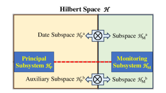
Figure 1: The decomposition construction of the Hilbert space.

In light of this requirement, $|\phi_{1}(t)\rangle\otimes|a(t)\rangle$, $|\phi_{2}(t)\rangle\otimes|a(t)\rangle$ and $|\phi_{b}(t)\rangle\otimes|b(t)\rangle$ consist of a set of orthonormal basis vectors in the Hilbert space $\mathcal{H}$. It is clear that this requirement establishes a connection between the date subspace $\mathcal{H}^{a}_{P}(t)$ and the monitoring subspace $\mathcal{H}^{a}_{M}(t)$, and simultaneously links the auxiliary subspace $\mathcal{H}^{b}_{P}(t)$ to the monitoring subspace $\mathcal{H}^{b}_{M}(t)$. As a consequence, it is now possible to mitigate the systematic amplitude error occurring on the quantum operation for the computational subspace by performing a conditional measurement or a postselection on the monitoring subsystem.

For our purpose, we suppose that $|\phi_{1}(t)\rangle\otimes|a(t)\rangle$, $|\phi_{2}(t)\rangle\otimes|a(t)\rangle$ and $|\phi_{b}(t)\rangle\otimes|b(t)\rangle$ are the solutions of the Schrödinger equation $i|\dot{\psi}(t)\rangle=H(t)|\psi(t)\rangle$, where $H(t)$ is the driving Hamiltonian governing the time evolution of the quantum system. As an example, we take the driving Hamiltonian as

$$H(t)=\Omega(t)|\phi_{b}(0)\rangle\langle\phi_{2}(0)|\otimes|b\rangle\langle a|+\mathrm{H.c.},$$ (2)

where $\Omega(t)$ is a time-dependent real parameter and $\mathrm{H.c.}$ represents the Hermitian conjugate term. For this Hamiltonian, the basis state $|\phi_{1}(0)\rangle\otimes|a\rangle$ is a dark state, which can be see from the fact that $H(t)|\phi_{1}(0)\rangle\otimes|a\rangle=0$. The evolution operator corresponding to the Hamiltonian reads

$$\mathcal{U}(t)= [|\phi_{1}(0)\rangle\langle\phi_{1}(0)|\otimes|a\rangle\langle a|+\cos\omega(t)[|\phi_{2}(0)\rangle\langle\phi_{2}(0)|$$

$$\otimes|a\rangle\langle a|+|\phi_{b}(0)\rangle\langle\phi_{b}(0)|\otimes|b\rangle\langle b|]-i\sin\omega(t)$$

$$\times[|\phi_{b}(0)\rangle\langle\phi_{2}(0)|\otimes|b\rangle\langle a|+\mathrm{H.c.}]$$ (3)

with $\omega(t)=\int^{t}_{0}\Omega(t^{\prime})dt^{\prime}$. If we require

$$\int^{\tau}_{0}\Omega(t)dt=\pi,$$ (4)

the above defined evolution operator then yields

$$\mathcal{U}(\tau)= \left[|\phi_{1}(0)\rangle\langle\phi_{1}(0)|-|\phi_{2}(0)\rangle\langle\phi_{2}(0)|\right]\otimes|a\rangle\langle a|$$

$$-|\phi_{b}(0)\rangle\langle\phi_{b}(0)|\otimes|b\rangle\langle b|.$$ (5)

Considering that the initial state in the principal subsystem resides in the computational subspace spanned by the basis $|\phi_{1}(0)\rangle$ and $|\phi_{2}(0)\rangle$, the unitary operation is actually equivalent to $\mathcal{U}(\tau)=[|\phi_{1}(0)\rangle\langle\phi_{1}(0)|-|\phi_{2}(0)\rangle\langle\phi_{2}(0)|]\otimes|a\rangle\langle a|$. Thereafter, the target operation can be obtained by tracing out $|a\rangle\langle a|$, which yields

$$U=|\phi_{1}(0)\rangle\langle\phi_{1}(0)|-|\phi_{2}(0)\rangle\langle\phi_{2}(0)|.$$ (6)

It defines a rotation operation about the axis determined by $\{|\phi_{1}(0)\rangle,|\phi_{2}(0)\rangle\}$ with an angle $\pi$. Especially, when $|\phi_{1}(0)\rangle$ and $|\phi_{1}(0)\rangle$ are set to $|\phi_{1}(0)\rangle=\cos(\theta/2)|0\rangle+\sin(\theta/2\exp(i\varphi)|1\rangle$ and $|\phi_{2}(0)\rangle=\sin(\theta/2)\exp(-i\varphi)|0\rangle-\cos(\theta/2)|1\rangle$, i.e., the eigenstates of $\boldsymbol{\mathrm{n}\cdot\sigma}$, the rotation axis along an arbitrary direction can be implemented.

Before proceeding further, we briefly demonstrate that the evolution operator in our scheme is a nonadiabatic holonomic operation. Nonadiabatic holonomic transformation arises from the time evolution of a quantum system with a subspace, for example the subspace $\mathcal{H}^{a}_{P}(t)\otimes\mathcal{H}^{a}_{M}(t)$ in the Hilbert space $\mathcal{H}$ of our scheme, satisfying the cyclic evolution condition

$$\sum^{L}_{k=1}|\phi_{k}(\tau)\rangle\langle\phi_{k}(\tau)|\otimes|a(\tau)\rangle\langle a(\tau)|$$

$$= \sum^{L}_{k=1}|\phi_{k}(0)\rangle\langle\phi_{k}(0)|\otimes|a(0)\rangle\langle a(0)|$$ (7)

and the parallel transport condition Sjoqvist ; Xu

$$\langle\phi_{k}(t)|\otimes\langle a(t)|H(t)|a(t)\rangle\otimes|\phi_{l}(t)\rangle=0.$$ (8)

The first condition guarantees that a quantum state in the desired subspace returns to the initial subspace and the second condition ensures that the unitary operator is purely geometric within the subspace. From Eq. (II), we can readily verify that the cyclic evolution condition is satisfied. Furthermore, using the commutation relation $[H(t),\mathcal{U}(t)]=0$, one can confirm that $\langle\phi_{k}(t)|\otimes\langle a(t)|H(t)|a(t)\rangle\otimes|\phi_{l}(t)\rangle=\langle\phi_{k}(0)|\otimes\langle a(0)|\mathcal{U}^{\dagger}(t)H(t)\mathcal{U}(t)|a(0)\rangle\otimes|\phi_{l}(0)\rangle=\langle\phi_{k}(0)|\otimes\langle a(0)|H(t)|a(0)\rangle\otimes|\phi_{l}(0)\rangle=0$, i.e, the parallel transport condition is also satisfied. The unitary time evolution considered above is hence a nonadiabatic holonomic operation.

The above discussion is the ideal case without any operational errors. In practice, it is difficult to execute perfect control on the quantum system. The imperfect control may lead to the quantum system over-evolving or under-evolving during the time evolution, resulting in the output state leaking into the entire Hilbert space (hence no longer purely geometrical). A typical control imperfection that induces leakage is the systematic amplitude error, which occurs in such a way that

$$\int^{\tau}_{0}\Omega(t)dt=\pi\rightarrow(1+\epsilon)\pi$$ (9)

owing to the imperfect controls of evolution time $\tau\rightarrow(1+\epsilon)\tau$ or amplitude parameter $\Omega(t)\rightarrow(1+\epsilon)\Omega(t)$. In this case, the resulting unitary operator is found to be

$$\mathcal{U}_{\epsilon}(\tau)= \left[|\phi_{1}(0)\rangle\langle\phi_{1}(0)|-\cos(\epsilon\pi)|\phi_{2}(0)\rangle\langle\phi_{2}(0)|\right]\otimes|a\rangle\langle a|$$

$$-\cos(\epsilon\pi)|\phi_{b}(0)\rangle\langle\phi_{b}(0)|\otimes|b\rangle\langle b|$$

$$-i\sin(\epsilon\pi)\big{[}|\phi_{2}(0)\rangle\langle\phi_{b}(0)|\otimes|a\rangle\langle b|$$

$$+|\phi_{b}(0)\rangle\langle\phi_{2}(0)|\otimes|b\rangle\langle a|\big{]}.$$ (10)

Still assuming that the initial state of principal subsystem resides in the computational subspace, we always consider following the initial state $|\psi(0)\rangle=[c_{1}|\phi_{1}(0)\rangle+c_{2}|\phi_{2}(0)\rangle]\otimes|a\rangle$, where $|c_{1}|^{2}+|c_{2}|^{2}=1$. To see clearly what the systematic ampluitude error may lead to, let us recall again that in the ideal case, the final state is given by $|\psi(\tau)\rangle=[c_{1}|\phi_{1}(0)\rangle-c_{2}|\phi_{2}(0)\rangle]\otimes|a\rangle$ and the target output state after performing a partial trace yields

$$|\phi(\tau)\rangle=c_{1}|\phi_{1}(0)\rangle-c_{2}|\phi_{2}(0)\rangle.$$ (11)

By contrast, in an nonideal case with the systematic amplitude error, the evolution state under the action of $\mathcal{U}_{\epsilon}(\tau)$ is in turn given by

$$|\psi_{\epsilon}(\tau)\rangle= [c_{1}|\phi_{1}(0)\rangle-c_{2}\cos(\epsilon\pi)|\phi_{2}(0)\rangle]\otimes|a\rangle$$

$$-ic_{2}\sin(\epsilon\pi)|\phi_{b}(0)\rangle\otimes|b\rangle.$$ (12)

Obviously, the systematic amplitude error leads to the evolution state leaking into the entire Hilbert space. However, our scheme is designed in such a way that we are allowed to monitor the impact of the systematic amplitude error on the minotor qubit and hence acquire indirectly some information about the quality of the operation. Specfically, at the end of the time evolution, we can always perform a projective measurement on the monitoring subsystem to project the state back to the initial computational subspace. This projective measurement yields

$$|\phi_{\epsilon}(\tau)\rangle=\frac{c_{1}|\phi_{1}(0)\rangle-c_{2}\cos(\epsilon\pi)|\phi_{2}(0)\rangle}{\sqrt{|c_{1}|^{2}+|c_{2}|^{2}\cos^{2}(\epsilon\pi)}}$$ (13)

when collapsing the monitor into the basis vector $|a\rangle$ and $|\bar{\phi}_{\epsilon}(\tau)\rangle=-|\phi_{b}(0)\rangle$ when collapsing the monitor into the basis vector $|b\rangle$. As a consequence, conditional on $|a\rangle$ is detected, we claim that the output state is obtained, reading $|\phi_{\epsilon}(\tau)\rangle$. The success probability of this postselection is $|c_{1}|^{2}+|c_{2}|^{2}\cos^{2}(\epsilon\pi)$. That is, in our scheme we need to select a posteriori measurement result of the monitor qubit so as to obtain the desired output state on the computational subspace.

Let us now compare what our scheme can acheive with what if we do not resort to the monitoring subsystem. If there is a systematic amplitude error as that in Eq. (9), the time evolution operator is given by

$$U^{\prime}_{\epsilon}(\tau)= |\phi_{1}(0)\rangle\langle\phi_{1}(0)|-\cos(\epsilon\pi)|\phi_{2}(0)\rangle\langle\phi_{2}(0)|$$

$$-\cos(\epsilon\pi)|\phi_{b}(0)\rangle\langle\phi_{b}(0)|-i\sin(\epsilon\pi)$$

$$\times\left[|\phi_{2}(0)\rangle\langle\phi_{b}(0)|+|\phi_{b}(0)\rangle\langle\phi_{2}(0)|\right].$$ (14)

For the same initial input state $|\phi(0)\rangle=c_{1}|\phi_{1}(0)\rangle+c_{2}|\phi_{2}(0)\rangle$ residing in the computational subspace, the output state under the action of $U^{\prime}_{\epsilon}$ then reads

$$|\phi^{\prime}_{\epsilon}(\tau)\rangle= c_{1}|\phi_{1}(0)\rangle-c_{2}\cos(\epsilon\pi)|\phi_{2}(0)\rangle$$

$$-ic_{2}\sin(\epsilon\pi)|\phi_{b}(0)\rangle.$$ (15)

As seen above, the systematic amplitude error causes the time evolving state to leak out of the computational subspace. However, in the plain version, there is no extra qubit tagging the unwanted amplitude on the state $|\phi_{b}(0)\rangle$.

To demonstrate the improvement of our nonadiabatic holonomic operation with a monitoring qubit, we compare fidelities $F=|\langle\phi_{\epsilon}(\tau)|\phi(\tau)\rangle|$ of our scheme with the reference plain scheme described above, where $|\phi_{\epsilon}(\tau)\rangle$ is the erroneous output state and $|\phi(\tau)\rangle$ is the target output state. A straightforward calculation based on Eqs. (11) and (13) yields that in our scheme, the fidelity is given by

$$F=\frac{|c_{1}|^{2}+|c_{2}|^{2}\cos(\epsilon\pi)}{\sqrt{|c_{1}|^{2}+|c_{2}|^{2}\cos^{2}(\epsilon\pi)}}.$$ (16)

In contrast, the fidelity of the reference scheme is obtained by combining Eqs. (11) and (II) as

$$F^{\prime}=|c_{1}|^{2}+|c_{2}|^{2}\cos(\epsilon\pi).$$ (17)

It is obvious that $F>F^{\prime}$. Evidently then, our scheme improves the fidelity of nonadiabatic holonomic operations on the computational space by introducing a conditional measurement on the monitor qubit.

To elucidate on the advantages of our approach, we plot the fidelities $F$ (the red line) and $F^{\prime}$ (the blue line) vs the error ratio $\epsilon$ in Fig. 2, setting $c_{1}=c_{2}=1/\sqrt{2}$ for convenience. The result shows that our scheme maintains high fidelity over the rang $\epsilon\in[0,0.3]$ compared with the reference scheme. This indicates that our scheme indeed considerably improves the fidelity of nonadiabatic holonomic operations. It is worth emphasizing that even for a relatively large value $\epsilon=0.3$, in the sense that the systematic amplitude error occurs in such a way that $\int^{\tau}_{0}\Omega(t)dt=\pi\rightarrow 1.3\pi$, the fidelity of our scheme still exceeds $95\%$ but the fidelity of the reference plain scheme is lower than $80\%$. This example indicates that the nonadiabatic holonomic operation in our scheme behaves well while the nonadiabatic holonomic operation in the reference scheme is strongly deteriorated by the systematic amplitude error.

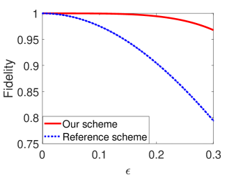
Figure 2: The fidelities of our scheme and the reference scheme.

To appreciate the benefits of our scheme more quantitatively, we present the computational results in Table 1. It shows that for the error parameter $\epsilon=0.05$, $0.1$, $0.15$ and $0.2$, the fidelity of our scheme can be up to $99.998\%$, $99.969\%$, $99.83\%$ and $99.45$, respectively, which is much higher than the corresponding fidelity $99.38\%$, $97.55\%$, $94.55\%$ and $90.45\%$ achieved in the reference scheme. This shows that our scheme has a significant improvement in the robustness against the systematic amplitude error.

Table 1: Computational results of our scheme and the reference scheme.

	$\epsilon$		$0.05$		$0.1$		$0.15$		$0.2$		$0.25$		$0.3$
	$F$		$99.998\%$		$99.969\%$		$99.83\%$		99.45%		$98.56\%$		$96.79\%$
	$F^{\prime}$		$99.38\%$		$97.55\%$		$94.55\%$		90.45%		$85.36\%$		$79.39\%$

III Realization in decoherence-free subspaces

Let us now turn to the quesiton how to realize our scheme in the decoherence-free subspace $\mathcal{H}=\mathrm{Span}\{|010\rangle,|100\rangle,|001\rangle\}$. The decoherence-free subspace not only provides a natural mathematical structure in Eq. (1), allowing us to use postselection to protect nonadiabatic holonomic operations against the fractional systematic amplitude error, but also gains their resilience to the collective dephasing induced by the interaction Hamiltonian

$$H_{\mathrm{int}}=\left[\sigma^{(1)}_{z}+\sigma^{(2)}_{z}+\sigma^{(3)}_{z}\right]\otimes{E},$$ (18)

where $E$ is the environment operator shared by all the three qubits Duan1997 ; Lidar ; Zanardi1997 . In the three-qubit decoherence-free subspace, the first two qubits are used as the principle subsystem such that $\mathcal{H}_{P}=\mathrm{Span}\{|01\rangle,|10\rangle,|00\rangle\}$ and the last qubit is used as the monitoring subsystem such that $\mathcal{H}_{A}=\mathrm{Span}\{|0\rangle,|1\rangle\}$. The computational qubit is encoded as $|0\rangle_{L}\equiv|01\rangle$ and $|1\rangle_{L}\equiv|10\rangle$ while the basis vector $|00\rangle$ acts as an ancilla. The Hamiltonian governing the time evolution of the quantum system is chosen as

$$H(t)=\sum_{k<l}\left[J^{x}_{kl}(t)R^{x}_{kl}+J^{y}_{kl}(t)R^{y}_{kl}\right],$$ (19)

where $J^{x}_{kl}(t)$ and $J^{y}_{kl}(t)$ are the coupling parameters corresponding to the $XY$ interaction $R^{x}_{kl}=[\sigma^{(k)}_{x}\sigma^{(l)}_{x}+\sigma^{(k)}_{y}\sigma^{(l)}_{y}]/2$ and the Dzialoshinski-Moriya interaction $R^{y}_{kl}=[\sigma^{(k)}_{x}\sigma^{(l)}_{y}-\sigma^{(k)}_{y}\sigma^{(l)}_{x}]/2$, respectively Yang ; Johnson ; Dzyaloshinsky ; Moriya ; Li ; Wu . For our purpose, we set the the non-zero coupling parameters as $J^{x}_{13}(t)=-J(t)\cos(\theta/2)$, $J^{x}_{23}(t)=J(t)\sin(\theta/2)\cos\varphi$ and $J^{y}_{13}(t)=J(t)\sin(\theta/2)\sin\varphi$. Then, we have

$$H(t)=J(t)|00\rangle\langle\Phi_{2}|\otimes|1\rangle\langle 0|+\mathrm{H.c.}$$ (20)

with $|\Phi_{2}\rangle=\sin(\theta/2)\exp(-i\varphi)|0\rangle_{L}-\cos(\theta/2)|1\rangle_{L}$. Note that the Hamiltonian $H(t)$ has a dark state $|\Phi_{1}\rangle\otimes|0\rangle=\cos(\theta/2)|0\rangle_{L}|0\rangle+\sin(\theta/2)\exp(i\varphi)|1\rangle_{L}|0\rangle$, where $|\Phi_{1}\rangle$ combines with $|\Phi_{2}\rangle$ making up of another basis in the computational space, such that $\mathcal{H}^{a}_{P}(0)=\mathrm{Span}\{|0\rangle_{L},|1\rangle_{L}\}=\mathrm{Span}\{|\Phi_{1}\rangle,|\Phi_{2}\rangle\}$. If we require $\int^{\tau}_{0}J(t)=\pi$, we have the evolution operator

$$\mathcal{U}=\left(|\Phi_{1}\rangle\langle\Phi_{1}|-|\Phi_{2}\rangle\langle\Phi_{2}|\right)\otimes|0\rangle\langle 0|-|00\rangle\langle 00|\otimes|1\rangle\langle 1|.$$ (21)

Recalling that the input states of the principle subsystem is in the computational space spanned by $\{|0\rangle_{L},|1\rangle_{L}\}$, the evolution operator is equivalent to $\mathcal{U}=(|\Phi_{1}\rangle\langle\Phi_{1}|-|\Phi_{2}\rangle\langle\Phi_{2}|)\otimes|0\rangle\langle 0|$. Therefore, the target nonadiabatic holonomic operation can be obtained by tracing out $|0\rangle\langle 0|$ after the time evolution, that is $U=|\Phi_{1}\rangle\langle\Phi_{1}|-|\Phi_{2}\rangle\langle\Phi_{2}|$. This is the ideal case without systematic amplitude errors.

If there is a systematic amplitude error $\epsilon$, unlike the ideal case, the evolution operator goes to an erroneous one

$$\mathcal{U}_{\epsilon}= \left[|\Phi_{1}\rangle\langle\Phi_{1}|-\cos(\epsilon\pi)|\Phi_{2}\rangle\langle\Phi_{2}|\right]\otimes|0\rangle\langle 0|$$

$$-\cos(\epsilon\pi)|00\rangle\langle 00|\otimes|1\rangle\langle 1|-i\sin(\epsilon\pi)|\Phi_{2}\rangle\langle 00|$$

$$\otimes|0\rangle\langle 1|-i\sin(\epsilon\pi)|00\rangle\langle\Phi_{2}|\otimes|1\rangle\langle 0|.$$ (22)

This erroneous time evolution operator takes the system initially in the computational space to a state eventually away from the computational subspace. However, upon performing a conditional measurement on the monitoring subsystem, we can obtain the output state closer to the target output state. For an input state $|\Psi(0)\rangle=(c_{1}|\Phi_{1}\rangle+c_{2}|\Phi_{2}\rangle)\otimes|0\rangle$, the output state is achieved as the following:

$$|\Phi_{\epsilon}\rangle=\frac{c_{1}|\Phi_{1}\rangle-c_{2}\cos(\epsilon\pi)|\Phi_{2}\rangle}{\sqrt{|c_{1}|^{2}+|c_{2}|^{2}\cos^{2}(\epsilon\pi)}}$$ (23)

conditional on $|0\rangle$ being detected. From the general discussions in the preceding section, we can easily conclude that this output state is much closer to the target output state $|\Phi(\tau)\rangle=c_{1}|\Phi_{1}\rangle-c_{2}|\Phi_{2}\rangle$ than the output state

$$|\Phi^{\prime}_{\epsilon}(\tau)\rangle=c_{1}|\Phi_{1}\rangle-c_{2}\cos(\epsilon\pi)|\Phi_{2}\rangle-ic_{2}\sin(\epsilon\pi)|00\rangle$$ (24)

obtained using the reference scheme. This ends our discussions on an explicit implementation of our scheme in a decoherence-free subspace.

IV Conclusion

In conclusion, we have proposed a scheme to protect nonadiabatic holonomic operations against the systematic amplitude error. Our scheme lies in introducing a conditional measurement on a monitor qubit. In essence, we have thus introduced a measurement-assisted approach to nonadiabatic holonomic operations. Furthermore, we have given a physical realization of our scheme in a decoherence-free subspace, making it not only robust against the systematic amplitude error but also resilient to some collective dephasing noise.

- (1) E. Hagley, X. Maitre, G. Nogues, C. Wunderlich, M. Brune, J. M. Raimond, and S. Hroche, Phys. Rev. Lett. 79, 1 (1997).
- (2) Q. A. Turchette, C. S. Wood, B. E. King, C. J. Myatt, D. Leibfried, W. M. Itano, C. Moroe, and D. J. Wineland, Phys. Rev. Lett. 81, 3631 (1998).
- (3) J. I. Cirac, P. Zoller, H.J. Kimble, and H. Mabuchi, Phys. Rev. Lett. 78, 3221 (1997).
- (4) K. Bergmann, H. Theuer, and B. W. Shore, Rev. Mod. Phys. 70, 1003 (1998).
- (5) C. H. Bennett, G. Brassard, C. Crepeau, R. Jozsa, A. Peres, and W. K. Wootters, Phys. Rev. Lett. 70, 1895 (1993).
- (6) D. Deutsch and R. Jozsa, Proc. R. Soc. London A 439, 553 (1992).
- (7) G. De Chiara and G. M. Palma, Phys. Rev. Lett. 91, 090404 (2003).
- (8) P. Solinas, P. Zanardi, and N. Zangh, Phys. Rev. A 70, 042316 (2004).
- (9) S. L. Zhu, Z. D. Wang, and P. Zanardi, Phys. Rev. Lett. 94, 100502 (2005).
- (10) C. Lupo, P. Aniello, M. Napolitano, and G. Florio, Phys. Rev. A 76, 012309 (2007).
- (11) S. Filipp, J. Klepp, Y. Hasegawa, C. Plonka-Spehr, U. Schmidt, P. Geltenbort, and H. Rauch, Phys. Rev. Lett. 102, 030404 (2009).
- (12) M. Johansson, E. Sjöqvist, L. M. Andersson, M. Ericsson, B. Hessmo, K. Singh, and D. M. Tong, Phys. Rev. A 86, 062322 (2012).
- (13) S. Berger, M. Pechal, A. A. Abdumalikov, J. C. Eichler, L. Steffen, A. Fedorov, A. Wallraff, and S. Filipp, Phys. Rev. A 87, 060303(R) (2013).
- (14) P. Zanardi and M. Rasetti, Phys. Lett. A 264, 94 (1999).
- (15) J. A. Jones, V. Vedral, A. Ekert, and G. Castagnoli, Nature 403, 869 (2000).
- (16) L. M. Duan, J. I. Cirac, and P. Zoller, Science 292, 1695 (2001).
- (17) M. V. Berry, Proc. R. Soc. London, Ser. A 392, 45 (1984).
- (18) F. Wilczek and A. Zee, Phys. Rev. Lett. 52, 2111 (1984).
- (19) A. Messiah, Quantum Mechanics (North-Holland Pub. Co., Amsterdam, 1962).
- (20) D. M. Tong, Phys. Rev. Lett. 104, 120401 (2010).
- (21) X. B. Wang and K. Matsumoto, Phys. Rev. Lett. 87, 097901 (2001).
- (22) S. L. Zhu and Z. D. Wang, Phys. Rev. Lett. 89, 097902 (2002).
- (23) Y. Aharonov and J. Anandan, Phys. Rev. Lett. 58, 1593 (1987).
- (24) E. Sjöqvist, D. M. Tong, L. M. Andersson, B. Hessmo, M. Johansson, and K. Singh, New J. Phys. 14, 103035 (2012).
- (25) G. F. Xu, J. Zhang, D. M. Tong, E. Sjöqvist, and L. C. Kwek, Phys. Rev. Lett. 109, 170501 (2012).
- (26) J. Anandan, Phys. Lett. A 133, 171 (1988).
- (27) G. F. Xu, C. L. Liu, P. Z. Zhao, and D. M. Tong, Phys. Rev. A 92, 052302 (2015).
- (28) E. Sjöqvist, Phys. Lett. A 380, 65 (2016).
- (29) E. Herterich and E. Sjöqvist, Phys. Rev. A 94, 052310 (2016).
- (30) P. Z. Zhao, K. Z. Li, G. F. Xu, and D. M. Tong, Phys. Rev. A 101, 062306 (2020).
- (31) J. Spiegelberg and E. Sjöqvist, Phys. Rev. A 88, 054301 (2013).
- (32) Z. T. Liang, Y. X. Du, W. Huang, Z. Y. Xue, and H. Yan, Phys. Rev. A 89, 062312 (2014).
- (33) J. Zhang, L. C. Kwek, E. Sjöqvist, D. M. Tong, and P. Zanardi, Phys. Rev. A 89, 042302 (2014).
- (34) Z. Y. Xue, J. Zhou, and Z. D. Wang, Phys. Rev. A 92, 022320 (2015).
- (35) Z. Y. Xue, J. Zhou, Y. M. Chu, and Y. Hu, Phys. Rev. A 94, 022331 (2016).
- (36) Z. Y. Xue, F. L. Gu, Z. P. Hong, Z. H. Yang, D. W. Zhang, Y. Hu, and J. Q. You, Phys. Rev. Appl. 7, 054022 (2017).
- (37) P. Z. Zhao, X. D. Cui, G. F. Xu, E. Sjöqvist, and D. M. Tong, Phys. Rev. A 96, 052316 (2017).
- (38) Z. P. Hong, B. J. Liu, J. Q. Cai, X. D. Zhang, Y. Hu, Z. D. Wang, and Z. Y. Xue, Phys. Rev. A 97, 022332 (2018).
- (39) T. Chen, J. Zhang, and Z. Y. Xue, Phys. Rev. A 98, 052314 (2018).
- (40) P. Z. Zhao, G. F. Xu, and D. M. Tong, Phys. Rev. A 99, 052309 (2019).
- (41) T. Chen, P. Shen, and Z. Y. Xue, Phys. Rev. Appl. 14, 034038 (2020).
- (42) S. Li and Z. Y. Xue, Phys. Rev. Appl. 16, 044005 (2021).
- (43) Y. Liang, P. Shen, T. Chen, and Z. Y. Xue, Phys. Rev. Appl. 17, 034015 (2022).
- (44) P. Z. Zhao and D. M. Tong, Phys. Rev. A 108, 012619 (2023).
- (45) B. J. Liu, X. K. Song, Z. Y. Xue, X. Wang, and M. H. Yung, Phys. Rev. Lett. 123, 100501 (2019).
- (46) J. Zhang, T. H. Kyaw, S. Filipp, L. C. Kwek, E. Sjöqvist, D. M. Tong, Phys. Rep. 1027, 1 (2023).
- (47) A. A. Abdumalikov, J. M. Fink, K. Juliusson, M. Pechal, S. Berger, A. Wallraff, and S. Filipp, Nature 496, 482 (2013).
- (48) G. R. Feng, G. F. Xu, and G. L. Long, Phys. Rev. Lett. 110, 190501 (2013).
- (49) C. Zu, W. B. Wang, L. He, W. G. Zhang, C. Y. Dai, F. Wang, and L. M. Duan, Nature 514, 72 (2014).
- (50) S. A. Camejo, A. Lazariev, S. W. Hell, and G. Balasubramanian, Nat. Commun. 5, 4870 (2014).
- (51) Y. Sekiguchi, N. Niikura, R. Kuroiwa, H. Kano, and H. Kosaka, Nat. Photonics 11, 309 (2017).
- (52) Y. Xu, W. Cai, Y. Ma, X. Mu, L. Hu, Tao Chen, H. Wang, Y. P. Song, Z. Y. Xue, Z. Q. Yin, and L. Sun, Phys. Rev. Lett. 121, 110501 (2018).
- (53) B. B. Zhou, P. C. Jerger, V. O. Shkolnikov, F. J. Heremans, G. Burkard, and D. D. Awschalom, Phys. Rev. Lett. 119, 140503 (2017).
- (54) K. Nagata, K. Kuramitani, Y. Sekiguchi, and H. Kosaka, Nat. Commun. 9, 3227 (2018).
- (55) G. F. Xu, P. Z. Zhao, T. H. Xing, E. Sjöqvist, and D. M. Tong, Phys. Rev. A 95, 032311 (2017).
- (56) N. Ramberg and E. Sjöqvist, Phys. Rev. Lett. 122, 140501 (2019).
- (57) L. M. Duan and G. C. Guo, Phys. Rev. Lett. 79, 1953 (1997).
- (58) P. Zanardi and M. Rasetti, Phys. Rev. Lett. 79, 3306 (1997).
- (59) D. A. Lidar, I. L. Chuang, and K. B. Whaley, Phys. Rev. Lett. 81, 2594 (1998).
- (60) C. N. Yang and C. P. Yang, Phys. Rev. 150, 321 (1966).
- (61) J. D. Johnson and M. McCoy, Phys. Rev. A 6, 1613 (1972).
- (62) L. Dzyaloshinsky, J. Phys. Chem. Solids 4, 241 (1958).
- (63) T. Moriya, Phys. Rev. Lett. 4, 228 (1960).
- (64) K. Z. Li, P. Z. Zhao, and D. M. Tong, Phys. Rev. Research 2, 023295 (2020).
- (65) X. Wu and P. Z. Zhao, Phys. Rev. A 102, 032627 (2020).