Orbital-rotated Fermi-Hubbard model as a benchmarking problem for quantum chemistry with the exact solution

Abstract

Evaluating the relative performance of different quantum algorithms for quantum computers is of great significance in the research of quantum algorithms. In this study, we consider the problem of quantum chemistry, which is considered one of the important applications of quantum algorithms. While evaluating these algorithms in systems with a large number of qubits is essential to see the scalability of the algorithms, the solvable models usually used for such evaluations typically have a small number of terms compared to the molecular Hamiltonians used in quantum chemistry. The large number of terms in molecular Hamiltonians is a major bottleneck when applying quantum algorithms to quantum chemistry. Various methods are being considered to address this problem, highlighting its importance in developing quantum algorithms for quantum chemistry. Based on these points, a solvable model with a number of terms comparable to the molecular Hamiltonian is essential to evaluate the performance of such algorithms. In this paper, we propose a set of exactly solvable Hamiltonians that has a comparable order of terms with molecular Hamiltonians by applying a spin-involving orbital rotation to the one-dimensional Fermi-Hubbard Hamiltonian. We verify its similarity to the molecular Hamiltonian from some prospectives and investigate whether the difficulty of calculating the ground-state energy changes before and after orbital rotation by applying the density matrix renormalization group up to 24 sites corresponding to 48 qubits. This proposal would enable proper evaluation of the performance of quantum algorithms for quantum chemistry, serving as a guiding framework for algorithm development.

I Introduction

In recent years, with the rapid progress of quantum computing, there has been extensive research focusing not only on the development of quantum computers but also on the exploration of quantum algorithms. Current quantum computers are called noisy intermediate-scale quantum (NISQ) [1] devices which have tens to hundreds of qubits without quantum error correction (QEC). In the future, fault-tolerant quantum computing (FTQC) is expected to be realized by implementing QEC.

Quantum chemistry is attracting attention as a promising application of quantum algorithms on quantum computers, and various studies have been actively conducted, including quantum algorithms based on FTQC [2, 3, 4, 5], and can be implemented in NISQ devices (NISQ algorithm) [6, 7, 8, 9, 10, 11, 12].

In investigating the practical application of quantum algorithms, it is important to benchmark the performance of these quantum algorithms. Various proposals of methods to benchmark NISQ algorithms have been proposed [13, 14, 15, 16, 17, 18, 19, 20, 21].

When we consider practical applications of quantum algorithms in quantum chemistry, it is crucial to benchmark various algorithms with large molecules that have many electrons. However, it is generally difficult to evaluate the performance of quantum algorithms on such large systems. This is because it is difficult to calculate the exact ground-state energy in large systems on classical computers, which means that it is difficult to prepare values to compare with those obtained by quantum algorithms. Typically, in such large systems, performance is evaluated by approximated ground-state energy by some other method.

One solution is to employ Hamiltonians for which exact ground-state energies can be computed efficiently on classical computers. For example, in fermion systems such as the one-dimensional Fermi-Hubbard (1D FH) model [22, 23, 24, 25], it is sometimes possible to calculate the exact ground-state energy by applying the Bethe ansatz method [26, 27, 28]. Then we can evaluate the performance of quantum algorithms in large systems by using the Hamiltonian and the exact ground-state energy.

Of course, it is necessary to consider the difference between such a solvable Hamiltonian and molecular Hamiltonians. One of the important differences is the number of terms in each Hamiltonian. While the 1D FH Hamiltonian has $\mathcal{O}(N)$ terms, molecular Hamiltonians have $\mathcal{O}(N^{4})$ terms where $N$ represents the number of sites for the 1D FH Hamiltonian and the number of molecular orbitals for molecular Hamiltonians.

The number of terms in Hamiltonians is closely related to the number of measurements required to measure the expectation value of the Hamiltonian. When we apply NISQ algorithms to molecular Hamiltonians, measuring the expectation values naively requires the measurement of $\mathcal{O}(N^{4})$ distinct fermionic operators. Due to this large number of measurements, for example, it is estimated in [29] that it will need several days to evaluate the expectation value of the Hamiltonian just one time to analyze the combustion energies of small organic molecules with sufficient accuracy with the speed of current devices. There have been various studies addressing the issue of dealing with a large number of measurements required for evaluating expectation values. In particular, grouping methods that group the terms contained in the Hamiltonian into sets of the simultaneously-measurable operators have been studied [30, 31, 32]. Since the 1D FH Hamiltonian contains only $\mathcal{O}(N)$ terms and the effectiveness of grouping methods is relatively small, comparing the performance of grouping methods using this Hamiltonian is difficult. Therefore, if there is a solvable Hamiltonian with a term of $\mathcal{O}(N^{4})$, it is possible to perform a more proper benchmark for quantum algorithms in quantum chemistry.

In this study, we introduce the orbital-rotated 1D FH Hamiltonian by using random $2N\times 2N$ unitary matrices. The number of terms of the Hamiltonian becomes $\mathcal{O}(N^{4})$, and since the value of the ground-state energy is invariant under orbital rotations with unitary matrices, the new Hamiltonian has the same ground-state energy value as the original 1D FH model, which is determined using the Bethe ansatz method efficiently with respect to system size. Thus, the Hamiltonian constructed by this method has $\mathcal{O}(N^{4})$ terms and is solvable. Another important point is that the use of unitary matrices for orbital rotations generally leads to Hamiltonians that include complex numbers, and accordingly, the wave functions representing energy eigenstates become complex as well. Conversely, when orbital rotations are carried out using real symmetric matrices, one obtains a real Hamiltonian, and the wave functions become real. While it is common to work with real wave functions in quantum chemistry, there are some situations that need to consider complex wave functions (e.g., considering magnetic field or the relativistic effect). Therefore, the ability to flexibly handle both real and complex wave functions by changing the rotation matrices used for orbital rotation is a useful feature in evaluating various quantum algorithms in quantum chemistry.

We investigate electronic correlation, an important property in quantum chemistry, for the orbital-rotated 1D FH Hamiltonian by applying the Hartree-Fock (HF) calculation and seeing electronic correlation energy defined as the difference between the HF energy and exact ground-state energy. Furthermore, we apply the well-known NISQ algorithm, the variational quantum eigensolver (VQE) [6] to the orbital-rotated 1D FH Hamiltonian and compare the result with the hydrogen chain (H-chain) Hamiltonian case. Finally, we apply the density matrix renormalization group (DMRG) [33, 34, 35, 36, 37] to the original 1D FH and orbital-rotated 1D FH Hamiltonians up to 24 sites corresponding to 48 qubits. By comparing the obtained ground-state energy with the exact ground energy from the Bethe ansatz method, we investigate whether the difficulty of calculating the ground-state energy changes before and after orbital rotation.

The rest of the paper is organized as follows. The orbital-rotated 1D FH Hamiltonian is introduced in Sec. II, and we investigate the similarity to the molecular Hamiltonian in Sec. III. A demonstration of the VQE and DMRG with the Hamiltonian is in Sec. IV. We conclude in Section V. Details of the setting of numerical simulations are given in the appendix.

II Hamiltonian

II.1 1D Fermi-Hubbard model

First, we start from the 1D FH Hamiltonian. This is given by

$$H = -t\sum_{i=0}^{N-1}\sum_{\sigma=\uparrow,\downarrow}(a^{\dagger}_{i,\sigma}a_{i+1,\sigma}+a^{\dagger}_{i+1,\sigma}a_{i,\sigma})$$ (1)

$$- \mu\sum_{i=0}^{N-1}\sum_{\sigma=\uparrow,\downarrow}a^{\dagger}_{i,\sigma}a_{i,\sigma}+U\sum_{i=0}^{N-1}a^{\dagger}_{i,\uparrow}a_{i,\uparrow}a^{\dagger}_{i,\downarrow}a_{i,\downarrow}$$

where $a^{\dagger}_{i,\sigma}$ and $a_{i,\sigma}$ are the creation and annihilation operators, respectively, for site $i$ and spin $\sigma$. $N$ represents the number of sites, $t$ is the tunneling amplitude, $\mu$ is the chemical potential, and $U$ is the Coulomb potential. In this paper, we restrict our discussion to the repulsive FH model ($U>0$). We set $t=1$ and impose the periodic boundary condition for simplicity. Although the Hamiltonian is expressed in terms of fermionic operators, it can be transformed into a qubit operator by employing fermion-qubit mappings such as the Jordan-Wigner mapping, resulting in a $2N$ qubits Hamiltonian.

Generally, the dimension of the Hamiltonian exponentially increases with the size of the system, making it extremely difficult to diagonalize and obtain the ground-state energy of Hamiltonians in large systems. In the 1D FH Hamiltonian, however, it is known that by using the Bethe Ansatz method, we can efficiently calculate the exact ground-state energy without diagonalizing the Hamiltonian even for such large systems  [26, 27, 28].

As mentioned in the introduction, when considering NISQ algorithms in quantum chemistry which are considered one of the useful applications, it is necessary to evaluate the performance of NISQ algorithms for molecular Hamiltonians with $\mathcal{O}(N^{4})$ terms. This includes a comparison of grouping methods for the reduction of the number of measurements, which is difficult to do with 1D FH with $\mathcal{O}(N)$ terms.

To address this issue, we consider spin-involved orbital rotations in the following sections of the paper.

II.2 Spin-involved orbital rotation

We introduce orbital rotations as a linear transformation of the creation and annihilation operators using a unitary matrix. Since in this study we consider orbital rotations that involve spins, we introduce a notation for the creation and annihilation operators as follows:

$$c_{2i}^{\dagger}=a_{i,\uparrow}^{\dagger},\quad c_{2i+1}^{\dagger}=a_{i,\downarrow}^{\dagger}$$ (2)

$$c_{2i}=a_{i,\uparrow},\quad c_{2i+1}=a_{i,\downarrow}.$$ (3)

Here $\uparrow(\downarrow)$ represents up (down) spin. The orbital-rotated operators $\tilde{c}_{i}^{\dagger}$ and $\tilde{c}_{i}$ are defined as follows:

$$\tilde{c}_{i}^{\dagger}=\sum_{k=0}^{2N-1}u_{ik}c_{k}^{\dagger},\quad\tilde{c}_{i}=\sum_{k=0}^{2N-1}u_{ik}^{*}c_{k}$$ (4)

where $*$ is the complex conjugate and $u_{ij}$ is a $2N\times 2N$ unitary matrix. From the form of the Hamiltonian, it can be observed that performing orbital rotations without mixing spin does not increase the number of terms. By performing this spin-involved orbital rotation, the 1D FH Hamiltonian can be expressed as

$$\tilde{H}=\sum_{p,q=0}^{2N-1}h_{pq}c^{\dagger}_{p}c_{q}+\frac{1}{2}\sum_{p,q,r,s=0}^{2N-1}h_{pqrs}c^{\dagger}_{p}c_{q}c^{\dagger}_{r}c_{s}.$$ (5)

Here, the coefficients $h_{pq}$, $h_{pqrs}$ are the one-body and two-body coefficients, respectively, and they are expressed as follows:

$$h_{pq} = -\sum_{i=0}^{N-1}(u_{2i,p}u_{2i+2,q}^{*}+u_{2i+2,p}u_{2i,q}^{*}$$ (6)

$$+ u_{2i+1,p}u_{2i+3,q}^{*}+u_{2i+3,p}u_{2i+1,q}^{*}+\mu\delta_{pq})\ \ \ \$$ (7)

$$h_{pqrs} = 2U\sum_{i=0}^{N-1}u_{2i,p}u_{2i,q}^{*}u_{2i+1,r}u_{2i+1,s}^{*}.$$ (8)

This form is the same as the second quantized molecular Hamiltonian in quantum chemistry and the number of terms is $\mathcal{O}(N^{4})$, allowing for a comparison of grouping methods.

In molecular Hamiltonians of quantum chemistry, the $z$-component of total electron spin $S_{z}$ is usually conserved. However, in the case of the orbital rotated 1D FH Hamiltonian, it is important to note that $S_{z}$ is not conserved due to the mixing of spins by the orbital rotation.

Since the creation and annihilation operators in (4) are rotated by using the unitary matrix, the spectrum of the energy eigenvalues is invariant under this orbital rotation. To see this, let us consider a transformation of the Hamiltonian with a unitary matrix $U(\kappa)$ in the following form:

$$\tilde{H}=U^{\dagger}(\kappa)HU(\kappa),\quad U(\kappa)=\exp{\left(\sum_{p,q=0}^{2N-1}\kappa_{pq}c^{\dagger}_{p}c_{q}\right)}$$ (9)

Here, $\kappa$ represents a set of $2N\times 2N$ real parameters, and due to the unitarity of $U$, we have $\kappa_{pq}=-\kappa_{qp}$. According to the Thouless theorem [38], this transformation is equivalent to the transformation (4) on the creation and annihilation operators when we choose $u$ as follows:

$$[\log u]_{pq}=\kappa_{pq}$$ (10)

where $[\log u]_{pq}$ is the $(p,q)$ element of the matrix $\log u$. Therefore, since the orbital rotation is represented as a similarity transformation on the Hamiltonian (9), the spectrum of the energy eigenvalues is invariant under this transformation.

As mentioned in the introduction, the orbital rotations by using unitary matrices generally lead to complex Hamiltonians and complex wave functions. Conversely, when orbital rotations are carried out using real symmetric matrices, one obtains a real Hamiltonian and the real wave functions. This is a useful feature in evaluating various NISQ algorithms in quantum chemistry.

III Similarity to molecule Hamiltonians

The Hamiltonian we have constructed consists of $\mathcal{O}(N^{4})$ terms, which is the same as molecular Hamiltonians. In this section, we further confirm the similarity to the molecular Hamiltonian from various perspectives. In the following sections, all orbital-rotated 1D FH Hamiltonians are constructed by applying the orbital rotation using the same $2N\times 2N$ unitary matrix and we set $\mu=U/2$. By choosing this particular value for $\mu$, the ground state of this system is known to be in a half-filled state [25] which has a number of electrons equal to the total number of sites. Each site can accommodate two electrons, so half of the maximum allowable number of electrons are filled. The details of the setting of all numerical simulations in this section are shown in Appendix A.

III.1 Hartree-Fock calculation and the electronic correlation

Here, we apply the HF calculation to the orbital-rotated 1D FH Hamiltonian and investigate the properties that relate to the electronic correlation in molecules. The HF calculation is a widely used approach in quantum chemistry to approximate the ground state of a molecular system. In the context of molecular Hamiltonians, it provides a mean-field description by assuming that each electron moves in an average field generated by all other electrons, neglecting electronic correlation which indicates the interactions among electrons. Due to the neglect of electronic correlation, the HF energy $E_{\mathrm{HF}}$ is always larger than the exact ground-state energy $E_{\mathrm{exact}}$. This energy difference is referred to as the correlation energy or electronic correlation energy $E_{\mathrm{corr}}$,

$$E_{\mathrm{corr}}=E_{\mathrm{exact}}-E_{\mathrm{HF}}.$$ (11)

To improve the HF calculation, it is important to account for the electronic correlation, and various methods, often referred to as post-Hartree-Fock methods, have been proposed.

Here we investigate the electronic correlation in the H-chain Hamiltonian and the orbital-rotated 1D FH Hamiltonian by using the electronic correlation energy $E_{\mathrm{corr}}$. By comparing with the Hamiltonian of H-chain, which is a widely used molecule for benchmarking, we illustrate the similarity of the orbital-rotated 1D FH Hamiltonian to the molecular Hamiltonian.

First, we perform HF calculation with the half-filled state. Since the spin $S_{z}$ is not conserving in the orbital-rotated 1D FH Hamiltonian, the HF calculation here is the unrestricted HF calculation with orbital rotations that take into account mixing of spins. Then we calculate and compare the electronic correlation energies of the orbital-rotated 1D FH Hamiltonian and the H-chain Hamiltonian that all hydrogen atoms are equally spaced with distance $R$. Figure 1 presents plots of electronic correlation energy as a function of atomic distance $R$ for the H-chain and as a function of the Coulomb potential $U$ for the orbital-rotated 1D FH Hamiltonian. From this figure, it can be seen that, just as the electronic correlation energy increases with increasing $R$ in the H-chain, the electronic correlation energy also increases with increasing $U$ in the orbital-rotated FH model.

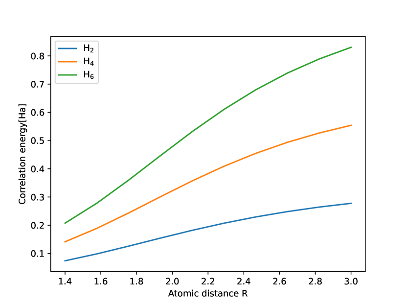
(a)

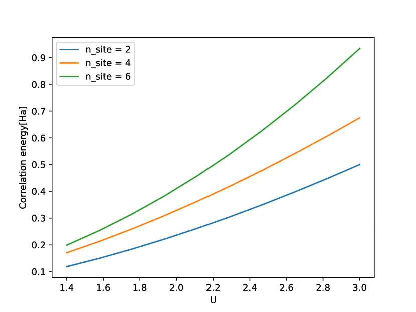
(b)

Figure 1: In (a), the electronic correlation energies of H2, H4, and H6 are plotted as functions of the atomic distance $R$. In (b), the electronic correlation energies of the orbital-rotated FH model with $N=2,4,6$ are plotted as functions of the $U$.

This can be understood by using the relation between the 1D FH model and the H-chain as follows. The FH model is known to be useful for describing strongly correlated electron systems (for example, see [39, 40, 41]), and the H-chain that all hydrogen atoms are equally spaced with distance is described by the 1D FH model [42]. Let us consider the situation where the atomic distance $R$ is large. In this case, electrons are localized on each atom, and in terms of the correspondence between the H-chain and the FH model, this corresponds to a situation where the tunneling amplitude $t$ (the transition amplitude of electrons between different atoms) is small in the FH model. With fixed $t$, the small $t$ implies the large Coulomb parameter $U$. A similar understanding can be applied when $R$ is small.

In some cases, the HF state exhibits degeneracy due to the symmetries present in the FH model before orbital rotation. For instance, when performing HF calculation on a four-site system, there is a degeneracy where four states yield the same HF energy. However, it should be noted that this degeneracy is dependent on the number of sites, as it is not observed in a six-site system.

III.2 Operator norm

In quantum chemistry, the atomic unit which uses the Hartree energy as the fundamental unit is commonly used. An important criterion for practical quantum computational chemistry is whether the measurement value obtained from the molecular Hamiltonian satisfies the chemical accuracy ($1.6\times 10^{-3}$ Hartree).

When considering the accuracy of measurements obtained from the orbital-rotated 1D FH in terms of chemical accuracy, it is necessary to align the scales of measurement values obtained with molecular Hamiltonians. This alignment ensures that the accuracy of the measurement values obtained by applying the quantum algorithm to the orbital-rotated 1D FH and molecular Hamiltonians will be on the same scale. This allows for a more appropriate evaluation of quantum chemical algorithms.

This is achieved by aligning the operator norm in both Hamiltonians. The operator norm in the molecular Hamiltonian depends on the molecular geometry and the chosen set of basis functions, while in the orbital-rotated FH Hamiltonian depends on $U$. Therefore, by adjusting $U$, it is possible to align the energy scales of both systems.

Figure 2 represents the comparison of the operator norm for H-chain, benzene, and the orbital-rotated 1D FH with several values of $U$. By adjusting $U$, it is possible to adjust the measurement values of the orbital-rotated 1D FH to the same order as those of molecular Hamiltonians. This figure indicates that the operator norm at $U=3$ is comparable to that of molecular Hamiltonians. Therefore, for subsequent numerical calculations, we set $U=3$.

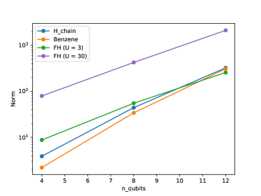
Figure 2: The results of operator norms calculated for H-chain (H2, H4, H6), benzene (with active spatial orbitals and active electrons numbers are $(2,2),(4,4),(6,6)$), and the orbital-rotated 1D FH model (with the number of sites are $2,4,6$).

III.3 Grouping

Since the orbital-rotated 1D FH Hamiltonian has $\mathcal{O}(N^{4})$ terms, the scaling of the number of groups obtained by applying the grouping methods is expected to be similar to the case of molecular Hamiltonians which have the same order of terms. We have compared various grouping methods, qubitwise commuting [30], general commuting [31] and basis rotation grouping [32], in the H-chain Hamiltonians and orbital-rotated 1D FH Hamiltonian. As a comparative measure, we have used the number of shots required for which the standard deviation of the expectation value of the ground-state energy estimations achieves chemical accuracy.

The required number of shots $M$ to achieve a certain accuracy $\epsilon$ is known to be given by the following equation:

$$M=\frac{K}{\epsilon^{2}}$$ (12)

where $K$ is a proportionality constant that depends on the Hamiltonian, shot allocation, and various other factors. We consider the optimal allocation of shots for the grouped Hamiltonian. The grouped Hamiltonian is denoted as

$$H=\sum_{G}\sum_{\alpha\in G}h_{\alpha}P_{\alpha}$$ (13)

where $P_{\alpha}$ are Pauli strings, $G$ labels groups and $\alpha$ labels terms in a group. Then $K$ is expressed as follows:

$$K=\left[\sum_{G}\sqrt{\sum_{\alpha,\beta}h_{\alpha}h_{\beta}\mathrm{Covar}(P_{\alpha},P_{\beta})}\right]^{2}.$$ (14)

Here $\mathrm{Covar}(P_{\alpha},P_{\beta})$ means the covariance between $P_{\alpha}$ and $P_{\beta}$ [43, 44].

We have estimated the number of shots for each grouping method up to $16$ qubits (Fig. 3). Here we have used exact ground states to calculate the variance and the covariance between Pauli strings. From these results, we can see that the number of shots required to achieve chemical accuracy exhibits a similar scaling for both the orbital-rotated 1D FH Hamiltonian and the actual molecular Hamiltonian. The performance of the basis rotation method has improved compared to the results obtained for the H-chain Hamiltonian. This is because the same operation as the orbit rotation used to construct the Hamiltonian is performed inside the basis rotation grouping, and this operation would reduce the number of terms increased by the orbital rotation. In fact, for small numbers of sites such as two-sites, after the basis rotation grouping the Hamiltonian has $\mathcal{O}(N)$ terms corresponding to the number of terms in the 1D FH Hamiltonian before the orbital rotation. An important point is that it is known that by applying the basis rotation grouping to the molecular Hamiltonian, only $\mathcal{O}(N)$ term groups remain [32] which are in the same order as the orbital-rotated 1D FH Hamiltonian case. This means that this $\mathcal{O}(N)$ scaling is not unique to the orbital-rotated 1D FH Hamiltonian.

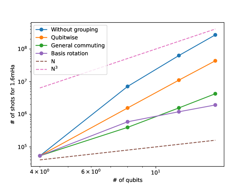
(a)

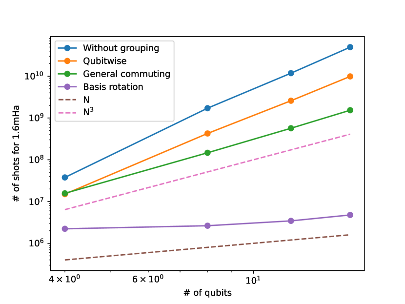
(b)

Figure 3: This is the comparison of various grouping methods, including qubitwise [30], general commuting [31] and basis rotation [32], applied to (a) the H chain and (b) the orbital-rotated FH model up to 16 qubits. The comparison metric is the number of shots required to achieve a chemical accuracy of $1.6$mHa for the calculated ground-state energy. The variance and covariance were calculated using the exact ground state.

IV Benckmark of algrotihms for finding ground state

In this section, we apply the VQE [6] to the orbital-rotated 1D FH Hamiltonian and compare the result with the H-chain Hamiltonian case. We then apply DMRG to both the original 1D FH Hamiltonian (Eq. 1) and the orbital-rotated 1D FH Hamiltonian to see if the difficulty of calculating the ground-state energy changes before and after orbital rotation.

IV.1 Variational Quantum Eigensolver

Here we apply the VQE with the H-chain Hamiltonian and the orbital-rotated 1D FH Hamiltonian to evaluate its performance. The VQE is an algorithm used to compute the ground-state energy using a quantum computer. We prepare a parametric quantum state, called the ansatz, represented as $|\psi(\vec{\theta})\rangle$. Here, $\theta$ is a set of parameters. The goal of the VQE is to approximate the ground state using this ansatz. The VQE is based on the variational principle, where the energy expectation value calculated with the ansatz is lower-bounded by the exact ground-state energy $E_{0}$ in the absence of statistical errors:

$$E(\vec{\theta})=\frac{\langle\psi(\vec{\theta})|H|\psi(\vec{\theta})\rangle}{\langle\psi(\vec{\theta})|\psi(\vec{\theta})\rangle}\geq E_{0}$$ (15)

For a given Hamiltonian $H$, we measure the energy expectation value $E(\vec{\theta})$ using a quantum computer. Then, we optimize the parameters $\theta$ using a classical optimization algorithm to minimize $E(\vec{\theta})$ and obtain the best approximation to the ground state. The gradient of the cost function required for optimization can be computed using the parameter shift rule [45].

The Hamiltonian of H-chains is prepared using the same settings as in Sec. III. The results under the hardware efficient (HE) ansatz [46] with different optimizers are presented in Fig. 4. Here we have compared optimizers including Adam [47], L-BFGS [48], Nakanishi-Fujii-Todo (NFT) [49], and simultaneous perturbation stochastic approximation (SPSA) [50]. All of these optimizers we have used in this simulation are implemented in QURI Parts [51], an open source library for developing quantum algorithms.

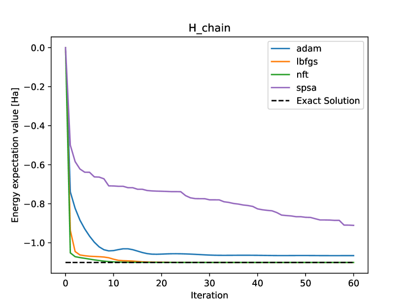
(a)

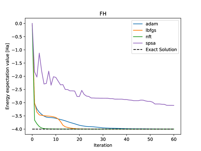
(b)

Figure 4: The results of the VQE with various optimizers, Adam [47], L-BFGS [48], NFT [49], and SPSA [50], applied to (a) the H2 molecule and (b) the two-site orbital-rotated 1D FH hamiltonian using the HE ansatz to see the behavior of each optimizer.

From these results, it can be seen that there are no significant differences in the convergence behavior for each optimizer between the H-chain and the orbital-rotated 1D FH Hamiltonian. Therefore, it would be possible to apply variational quantum algorithms such as the VQE with various optimizers to the orbital-rotated 1D FH Hamiltonian to investigate the performance of these algorithms for molecular Hamiltonians such as H-chain.

IV.2 DMRG

Here we apply DMRG [33, 34] to both the original 1D FH Hamiltonian (Eq. 1) and the orbital-rotated 1D FH Hamiltonian to see if the difficulty of calculating the ground-state energy changes before and after orbital rotation. The DMRG is a variational approach used to determine the ground state of quantum systems, and can also be formulated on the Matrix Product State (MPS) representation of quantum states [35, 36, 37]. Given MPS’s suitability for representing ground states of 1D Hamiltonians, DMRG is generally considered an optimal technique for finding ground states of one-dimensional lattice models that describe strongly correlated phenomena in solid-state physics. Its applicability to quantum chemical calculations was demonstrated in [52], and there have been various developments of practical quantum chemical computation using DMRG with the recent powerful classical computing resources. Here the DMRG calculations were performed using the MPS-based finite-system DMRG.

Figure 5 presents a comparison of the energy obtained through DMRG and the exact values for both the original 1D FH Hamiltonian and the orbital-rotated 1D FH Hamiltonian. The plotted data illustrates the energy differences $E_{\mathrm{diff}}$ between these energy values for systems up to 24 sites corresponding to 48 qubits, as defined below

$$E_{\mathrm{diff}}=\frac{E_{\mathrm{DMRG}}-E_{\mathrm{exact}}}{E_{\mathrm{exact}}}$$ (16)

where $E_{\mathrm{DMRG}}$ is the ground-state energy obtained from DMRG and $E_{\mathrm{exact}}$ is the exact ground-state energy. We conducted DMRG using the MPS ansatz with maximum bond-dimensions of $50$, $100$ and $500$, respectively only for even numbers of sites (i.e., the number of qubits is a multiple of 4). Here we have used ITensor [53] to conduct DMRG. The details of the setting of DMRG calculation in this section are shown in Appendix A.2.

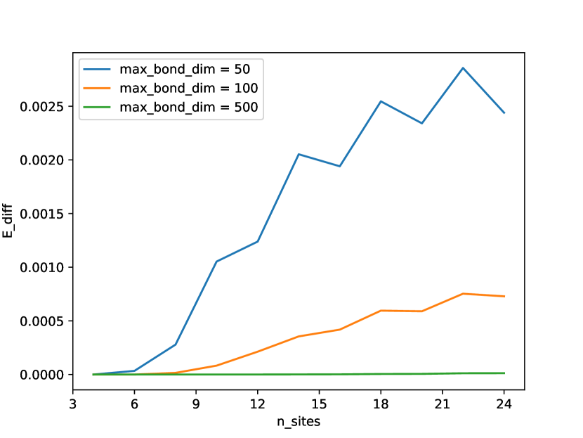
(a)

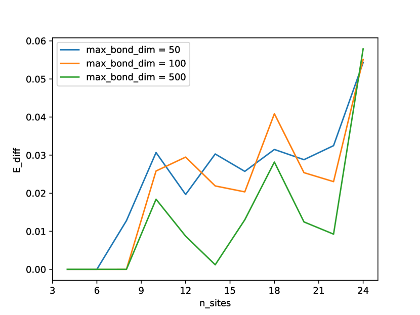
(b)

Figure 5: The results of differences $E_{\mathrm{diff}}$ of (a) the original 1D FH Hamiltonian and (b) the orbital-rotated 1D FH Hamiltonian, obtained from the energy by using the MPS-based finite-system DMRG for MPS bond dimensions of 50, 100, and 500 and the exact ground-state energy up to 24 sites. The exact energy values were derived using the Bethe ansatz.

From these results, it can be seen that increasing the maximum bond dimension leads to improved accuracy in the ground-state energy obtained from DMRG for the original 1D FH Hamiltonian. On the other hand, in the orbital-rotated 1D FH Hamiltonian, there is not a significant difference in the accuracy of the DMRG energy when the maximum bond dimension increases from 50 to $100$ but slightly improves when the bond dimension is allowed up to $500$. Furthermore, by comparing $E_{\mathrm{diff}}$ of both Hamiltonians, it can be seen that orbital rotation decreases the accuracy of the energy obtained by DMRG, implying that the orbital rotation can make the problem harder and more suitable for benchmarking.

V Conclusion

In this work, we have proposed the orbital-rotated 1D FH Hamiltonian for benchmarking purposes. One can calculate the exact ground-state energy of the Hamiltonian even for large systems, which allows us to investigate the performance of the quantum algorithms even in systems with a large number of qubits. Additionally, this Hamiltonian has $\mathcal{O}(N^{4})$ terms and thus allows us to investigate the performance of grouping methods that are important for reducing the number of measurements.

We have investigated the similarity with the molecular Hamiltonian in various ways. By comparing electronic correlation energies, we have confirmed the relation between the atomic distance in the H-chain Hamiltonian and the Coulomb parameter of the orbital-rotated 1D FH Hamiltonian.

Additionally, we have applied the VQE and compared results for the orbital-rotated 1D FH Hamiltonian and the H-chain Hamiltonian. From these results, it is confirmed that there are no significant differences between these Hamiltonians.

Finally, we have applied the DMRG to the original 1D FH Hamiltonian and orbital-rotated one. By comparing these results, we have verified that the orbital rotation can make the problem harder and more suitable for benchmarking.

In future work, it is interesting to evaluate whether DMRG is appropriate for the system by examining the entanglement entropy of the ground-state wavefunction [54]. This wavefunction of the orbital-rotated 1D FH Hamiltonian can be obtained by applying the Bethe Ansatz method. It may be worthwhile to conduct this evaluation on a system with a small number of sites. Furthermore, by using this ground-state wavefunction, there is a possibility of evaluating the performance of quantum algorithms that calculate other physical quantities obtained from the wavefunction. These are left for future work.

VI Acknowledgements

The authors would like to thank Kosuke Mitarai and Wataru Mizukami for their valuable discussion while formulating the problem. The authors also thank Ming-Zhi Chung, Ryosuke Imai, Shoichiro Tsutsui, Yuichiro Hidaka and Yuya O. Nakagawa for valuable information and comments. This work was performed for Council for Science, Technology and Innovation (CSTI), Cross-ministerial Strategic Innovation Promotion Program (SIP), “Photonics and Quantum Technology for Society 5.0”(Funding agency : QST).

Appendix A Details of numerical simulations

A.1 General setup

All numerical simulations have been conducted by using QURI Parts [51], an open source library for developing quantum algorithms. The orbital-rotated 1D FH Hamiltonian in this paper was constructed as follows. First, we generate the 1D FH Hamiltonian represented by annihilation and creation operators using OpenFermion [55]. Throughout this paper, all orbital-rotated 1D FH Hamiltonians are constructed by applying the orbital rotation using the same single unitary matrix randomly generated using SciPy [56]. For all orbital-rotated FH Hamiltonians in this paper, we set $U=3$ to align the operator norm wih molecular Hamiltonians, and $\mu=U/2=3/2$, resulting in the ground state being a half-filled state.

For all molecular Hamiltonians in this paper, we use the second-quantized electronic Hamiltonian using the Born-Oppenheimer approximation with Hartree-Fock orbitals. These are constructed by PySCF [57] with the STO-3G minimal basis set and then converted into qubit Hamiltonians through the Jordan-Wigner mapping. Molecular geometries used in this paper are shown in Table 1. The geometry of benzene is taken from the PubChem database [58].

Molecule	Geometry
Hn	(H, (0, 0, 0)), (H, (0, 0, 1.0)), …, (H, (0, 0, $n\times 1.0$))
Benzene	(C, (-1.2131, -0.6884, 0)), (C, (-1.2028, 0.7064, 0.0001)), (C, (-0.0103, -1.3948, 0)), (C, (0.0104, 1.3948, -0.0001)), (C, (1.2028, -0.7063, 0)), (C, (1.2131, 0.6884, 0)), (H, (-2.1577, -1.2244, 0)), (H, (-2.1393, 1.2564, 0.0001)), (H, (-0.0184, -2.4809, -0.0001)), (H, (0.0184, 2.4808, 0)), (H, (2.1394, -1.2563, 0.0001)), (H, (2.1577, 1.2245, 0))

Table 1: Molecular geometries are denoted as “($\mathrm{X}$, $(x,y,z))$,” where the 3D coordinates $x$, $y$, and $z$ of atom $\mathrm{X}$ are written in units of angstroms Å.

A.2 Details of the DMRG

The DMRG calculation in Sec. IV.2 is conducted by using the dmrg function in ITensor [53]. We have set the HF state as the initial state and performed a total of $10$ sweeps in the DMRG algorithm. The value of the truncation error cutoff to use for truncating the bond dimension or rank of the MPS was set to $10^{-8}$. The minimum size of the bond dimension was set to $10$ and the maximum sizes were set as $50,100,500$.

References

- Preskill [2018] J. Preskill, Quantum Computing in the NISQ era and beyond, Quantum 2, 79 (2018).
- Aspuru-Guzik et al. [2005] A. Aspuru-Guzik, A. D. Dutoi, P. J. Love, and M. Head-Gordon, Simulated quantum computation of molecular energies, Science 309, 1704 (2005).
- Wang et al. [2008] H. Wang, S. Kais, A. Aspuru-Guzik, and M. R. Hoffmann, Quantum algorithm for obtaining the energy spectrum of molecular systems, Physical Chemistry Chemical Physics 10, 5388 (2008).
- Poulin et al. [2014] D. Poulin, M. B. Hastings, D. Wecker, N. Wiebe, A. C. Doherty, and M. Troyer, The trotter step size required for accurate quantum simulation of quantum chemistry, arXiv preprint arXiv:1406.4920 (2014).
- Babbush et al. [2015] R. Babbush, J. McClean, D. Wecker, A. Aspuru-Guzik, and N. Wiebe, Chemical basis of trotter-suzuki errors in quantum chemistry simulation, Physical Review A 91, 022311 (2015).
- Peruzzo et al. [2014] A. Peruzzo, J. McClean, P. Shadbolt, M.-H. Yung, X.-Q. Zhou, P. J. Love, A. Aspuru-Guzik, and J. L. O’brien, A variational eigenvalue solver on a photonic quantum processor, Nature communications 5, 4213 (2014).
- Wecker et al. [2015] D. Wecker, M. B. Hastings, and M. Troyer, Progress towards practical quantum variational algorithms, Physical Review A 92, 042303 (2015).
- Cao et al. [2019] Y. Cao, J. Romero, J. P. Olson, M. Degroote, P. D. Johnson, M. Kieferová, I. D. Kivlichan, T. Menke, B. Peropadre, N. P. Sawaya, et al., Quantum chemistry in the age of quantum computing, Chemical reviews 119, 10856 (2019).
- McArdle et al. [2020] S. McArdle, S. Endo, A. Aspuru-Guzik, S. C. Benjamin, and X. Yuan, Quantum computational chemistry, Reviews of Modern Physics 92, 015003 (2020).
- Cerezo et al. [2021] M. Cerezo, A. Arrasmith, R. Babbush, S. C. Benjamin, S. Endo, K. Fujii, J. R. McClean, K. Mitarai, X. Yuan, L. Cincio, et al., Variational quantum algorithms, Nature Reviews Physics 3, 625 (2021).
- Bharti et al. [2022] K. Bharti, A. Cervera-Lierta, T. H. Kyaw, T. Haug, S. Alperin-Lea, A. Anand, M. Degroote, H. Heimonen, J. S. Kottmann, T. Menke, et al., Noisy intermediate-scale quantum algorithms, Reviews of Modern Physics 94, 015004 (2022).
- Tilly et al. [2022] J. Tilly, H. Chen, S. Cao, D. Picozzi, K. Setia, Y. Li, E. Grant, L. Wossnig, I. Rungger, G. H. Booth, et al., The variational quantum eigensolver: a review of methods and best practices, Physics Reports 986, 1 (2022).
- Amico et al. [2023] M. Amico, H. Zhang, P. Jurcevic, L. S. Bishop, P. Nation, A. Wack, and D. C. McKay, Defining standard strategies for quantum benchmarks, arXiv preprint arXiv:2303.02108 (2023).
- Lubinski et al. [2023a] T. Lubinski, S. Johri, P. Varosy, J. Coleman, L. Zhao, J. Necaise, C. H. Baldwin, K. Mayer, and T. Proctor, Application-oriented performance benchmarks for quantum computing, IEEE Transactions on Quantum Engineering (2023a).
- Lubinski et al. [2023b] T. Lubinski, C. Coffrin, C. McGeoch, P. Sathe, J. Apanavicius, and D. E. B. Neira, Optimization applications as quantum performance benchmarks, arXiv preprint arXiv:2302.02278 (2023b).
- Lubinski et al. [2024] T. Lubinski et al., Quantum Algorithm Exploration using Application-Oriented Performance Benchmarks, (2024), arXiv:2402.08985 [quant-ph] .
- Dutt et al. [2023] A. Dutt, W. Kirby, R. Raymond, C. Hadfield, S. Sheldon, I. L. Chuang, and A. Mezzacapo, Practical benchmarking of randomized measurement methods for quantum chemistry hamiltonians, arXiv preprint arXiv:2312.07497 (2023).
- Wu et al. [2023] D. Wu, R. Rossi, F. Vicentini, N. Astrakhantsev, F. Becca, X. Cao, J. Carrasquilla, F. Ferrari, A. Georges, M. Hibat-Allah, et al., Variational benchmarks for quantum many-body problems, arXiv preprint arXiv:2302.04919 (2023).
- [19] J. Finzgar, P. Ross, J. Klepsch, and A. Luckow, Quark: A framework for quantum computing application benchmarking (2022), arXiv preprint arXiv:2202.03028 .
- Gard and Meier [2022] B. T. Gard and A. M. Meier, Classically efficient quantum scalable fermi-hubbard benchmark, Physical Review A 105, 042602 (2022).
- Kobayashi et al. [2022] F. Kobayashi, K. Mitarai, and K. Fujii, Parent hamiltonian as a benchmark problem for variational quantum eigensolvers, Physical Review A 105, 052415 (2022).
- Hubbard [1964] J. Hubbard, Electron correlations in narrow energy bands. ii. the degenerate band case, Proceedings of the Royal Society of London. Series A. Mathematical and Physical Sciences 277, 237 (1964).
- Gutzwiller [1963] M. C. Gutzwiller, Effect of correlation on the ferromagnetism of transition metals, Physical Review Letters 10, 159 (1963).
- Kanamori [1963] J. Kanamori, Electron correlation and ferromagnetism of transition metals, Progress of Theoretical Physics 30, 275 (1963).
- Essler et al. [2005] F. H. Essler, H. Frahm, F. Göhmann, A. Klümper, and V. E. Korepin, The one-dimensional Hubbard model (Cambridge University Press, 2005).
- Lieb and Wu [1968] E. H. Lieb and F.-Y. Wu, Absence of mott transition in an exact solution of the short-range, one-band model in one dimension, Physical Review Letters 20, 1445 (1968).
- Lieb and Wu [2003] E. H. Lieb and F. Wu, The one-dimensional hubbard model: a reminiscence, Physica A: statistical mechanics and its applications 321, 1 (2003).
- Yang [1967] C.-N. Yang, Some exact results for the many-body problem in one dimension with repulsive delta-function interaction, Physical Review Letters 19, 1312 (1967).
- Gonthier et al. [2022a] J. F. Gonthier, M. D. Radin, C. Buda, E. J. Doskocil, C. M. Abuan, and J. Romero, Measurements as a roadblock to near-term practical quantum advantage in chemistry: Resource analysis, Phys. Rev. Res. 4, 033154 (2022a).
- McClean et al. [2016] J. R. McClean, J. Romero, R. Babbush, and A. Aspuru-Guzik, The theory of variational hybrid quantum-classical algorithms, New Journal of Physics 18, 023023 (2016).
- Gokhale et al. [2019] P. Gokhale, O. Angiuli, Y. Ding, K. Gui, T. Tomesh, M. Suchara, M. Martonosi, and F. T. Chong, Minimizing state preparations in variational quantum eigensolver by partitioning into commuting families, arXiv preprint arXiv:1907.13623 (2019).
- Huggins et al. [2021] W. J. Huggins, J. R. McClean, N. C. Rubin, Z. Jiang, N. Wiebe, K. B. Whaley, and R. Babbush, Efficient and noise resilient measurements for quantum chemistry on near-term quantum computers, npj Quantum Information 7, 23 (2021).
- White [1992] S. R. White, Density matrix formulation for quantum renormalization groups, Physical review letters 69, 2863 (1992).
- White [1993] S. R. White, Density-matrix algorithms for quantum renormalization groups, Physical review b 48, 10345 (1993).
- Östlund and Rommer [1995] S. Östlund and S. Rommer, Thermodynamic limit of density matrix renormalization, Physical review letters 75, 3537 (1995).
- Dukelsky et al. [1998] J. Dukelsky, M. A. Martín-Delgado, T. Nishino, and G. Sierra, Equivalence of the variational matrix product method and the density matrix renormalization group applied to spin chains, Europhysics letters 43, 457 (1998).
- Schollwöck [2011] U. Schollwöck, The density-matrix renormalization group in the age of matrix product states, Annals of physics 326, 96 (2011).
- Thouless [1960] D. J. Thouless, Stability conditions and nuclear rotations in the hartree-fock theory, Nuclear Physics 21, 225 (1960).
- Imada et al. [1998] M. Imada, A. Fujimori, and Y. Tokura, Metal-insulator transitions, Reviews of modern physics 70, 1039 (1998).
- Georges et al. [1996] A. Georges, G. Kotliar, W. Krauth, and M. J. Rozenberg, Dynamical mean-field theory of strongly correlated fermion systems and the limit of infinite dimensions, Reviews of Modern Physics 68, 13 (1996).
- Mielke and Tasaki [1993] A. Mielke and H. Tasaki, Ferromagnetism in the hubbard model: Examples from models with degenerate single-electron ground states, Communications in mathematical physics 158, 341 (1993).
- Sawaya and White [2021] R. C. Sawaya and S. R. White, Constructing hubbard models for the hydrogen chain using sliced basis dmrg, arXiv preprint arXiv:2109.05129 (2021).
- Rubin et al. [2018] N. C. Rubin, R. Babbush, and J. McClean, Application of fermionic marginal constraints to hybrid quantum algorithms, New Journal of Physics 20, 053020 (2018).
- Gonthier et al. [2022b] J. F. Gonthier, M. D. Radin, C. Buda, E. J. Doskocil, C. M. Abuan, and J. Romero, Measurements as a roadblock to near-term practical quantum advantage in chemistry: resource analysis, Physical Review Research 4, 033154 (2022b).
- Mitarai et al. [2018] K. Mitarai, M. Negoro, M. Kitagawa, and K. Fujii, Quantum circuit learning, Phys. Rev. A 98, 032309 (2018).
- Kandala et al. [2017] A. Kandala, A. Mezzacapo, K. Temme, M. Takita, M. Brink, J. M. Chow, and J. M. Gambetta, Hardware-efficient variational quantum eigensolver for small molecules and quantum magnets, nature 549, 242 (2017).
- Kingma and Ba [2014] D. P. Kingma and J. Ba, Adam: A method for stochastic optimization, arXiv preprint arXiv:1412.6980 (2014).
- Liu and Nocedal [1989] D. C. Liu and J. Nocedal, On the limited memory bfgs method for large scale optimization, Mathematical programming 45, 503 (1989).
- Nakanishi et al. [2020] K. M. Nakanishi, K. Fujii, and S. Todo, Sequential minimal optimization for quantum-classical hybrid algorithms, Physical Review Research 2, 043158 (2020).
- Spall [1998] J. C. Spall, Implementation of the simultaneous perturbation algorithm for stochastic optimization, IEEE Transactions on aerospace and electronic systems 34, 817 (1998).
- qur [2022] QURI Parts (2022), https://github.com/QunaSys/quri-parts.
- White and Martin [1999] S. R. White and R. L. Martin, Ab initio quantum chemistry using the density matrix renormalization group, The Journal of chemical physics 110, 4127 (1999).
- Fishman et al. [2022] M. Fishman, S. White, and E. Stoudenmire, The itensor software library for tensor network calculations, SciPost Physics Codebases , 004 (2022).
- Eisert et al. [2010] J. Eisert, M. Cramer, and M. B. Plenio, Colloquium: Area laws for the entanglement entropy, Reviews of modern physics 82, 277 (2010).
- McClean et al. [2020] J. R. McClean, N. C. Rubin, K. J. Sung, I. D. Kivlichan, X. Bonet-Monroig, Y. Cao, C. Dai, E. S. Fried, C. Gidney, B. Gimby, et al., Openfermion: the electronic structure package for quantum computers, Quantum Science and Technology 5, 034014 (2020).
- Virtanen et al. [2020] P. Virtanen, R. Gommers, T. E. Oliphant, M. Haberland, T. Reddy, D. Cournapeau, E. Burovski, P. Peterson, W. Weckesser, J. Bright, S. J. van der Walt, M. Brett, J. Wilson, K. J. Millman, N. Mayorov, A. R. J. Nelson, E. Jones, R. Kern, E. Larson, C. J. Carey, İ. Polat, Y. Feng, E. W. Moore, J. VanderPlas, D. Laxalde, J. Perktold, R. Cimrman, I. Henriksen, E. A. Quintero, C. R. Harris, A. M. Archibald, A. H. Ribeiro, F. Pedregosa, P. van Mulbregt, and SciPy 1.0 Contributors, SciPy 1.0: Fundamental Algorithms for Scientific Computing in Python, Nature Methods 17, 261 (2020).
- Sun et al. [2018] Q. Sun, T. C. Berkelbach, N. S. Blunt, G. H. Booth, S. Guo, Z. Li, J. Liu, J. D. McClain, E. R. Sayfutyarova, S. Sharma, et al., Pyscf: the python-based simulations of chemistry framework, Wiley Interdisciplinary Reviews: Computational Molecular Science 8, e1340 (2018).
- Kim et al. [2023] S. Kim, J. Chen, T. Cheng, A. Gindulyte, J. He, S. He, Q. Li, B. A. Shoemaker, P. A. Thiessen, B. Yu, et al., Pubchem 2023 update, Nucleic acids research 51, D1373 (2023).