The Price of Information

Abstract

When an investor is faced with the option to purchase additional information regarding an asset price, how much should she pay? To address this question, we solve for the indifference price of information in a setting where a trader maximizes her expected utility of terminal wealth over a finite time horizon. If she does not purchase the information, then she solves a partial information stochastic control problem, while, if she does purchase the information, then she pays a cost and receives partial information about the asset’s trajectory. We further demonstrate that when the investor can purchase the information at any stopping time prior to the end of the trading horizon, she chooses to do so at a deterministic time.

60G15, 91B24, 91B70, 93E11, 93E20

1 Introduction

When stock returns are predictable, the trading signal and the anticipation of future signals affect investor’s trading strategies [15, 19]. Without access to the trading signal, rational investors may still trade strategically by filtering the trading signal [1, 4, 10, 11] – i.e., treat the optimization problem as a partial information control problem. As an investor with full information always has higher utility than those without the full information [5, 11, 12], possessing information about the trading signal has a strictly positive value. The investor, therefore, has a maximum price that she is willing to pay to acquire this additional information.

Further, consider a group of informed traders who have access to partial information regarding the trading signal. Often there are regulatory constraints that prevent them from legally participating in the market. They can, however, form an information agency (IA) to “sell” some aspect of the trading signal that they possess to other investors. The maximum price an investor is willing to pay for this information may be viewed as the maximum price that the IA can sell the information to the investor.

In this article, we refer to this maximum price as the “indifference price”. In particular, the indifference price is the price that the investor is willing to pay such that their expected utility from optimally investing and filtering the trading signal (i.e., in the absence of the information) equals the expected utility from paying the indifference price, receiving the information, and then optimally trading with the information (i.e., in the presence of full information). Naturally, the investor will accept any price below the indifference price and will reject any price above the indifference price.

Our main goal is to address the question: how does an investor quantify the price of the trading signal? We show that, on a fixed trading horizon $[0,T]$, an investor with constant absolute risk aversion (CARA) has two parameters that affect their indifference price: (i) the investor’s risk aversion coefficient and (ii) the signal-to-noise ratio (or more specifically, the signal-to-volatility ratio). Further, we investigate the question of timing: when should the investor subscribe to the trading signal (until the end of the time horizon)? We show that if the investor is allowed to choose a stopping time at which to subscribe to the trading signal (and keep her subscription to the terminal time $T$), then, somewhat surprisingly, the optimal stopping time is a deterministic stopping time.

The remainder of the paper is organized as follows. In Section 2, we develop a single-period model, derive the participating investor’s optimal informed and uninformed trading strategy, and obtain the closed form expression for the indifference price. In Section 3, we develop the continuous time analogue of the model, and once again determine the indifference price in closed form and derive a limiting subscription rate for subscribing to the information when the time horizon is large. Finally, we consider the optimal subscription time problem in Section 4. All proofs are found in Appendix A.

Throughout, we fix a filtered probability space $(\Omega,{\mathcal{F}},\{{\mathcal{F}}_{t}\}_{{t\in{\mathfrak{T}}}},\mathbb{P})$ supporting two independent standard Brownian motions, $(B_{t}^{Y})_{{t\in{\mathfrak{T}}}}$ and $(B_{t}^{Z})_{{t\in{\mathfrak{T}}}}$, and ${\mathfrak{T}}:=[0,T]$ being the trading horizon. We use ${\mathcal{A}}(X)$ to denote the collection of all processes adapted to the filtration generated by the process $X$.

2 A Single-Period Model

We introduce the essential ideas in a single-period model.

2.1 Single-Period Model Setup

Suppose interest rates are zero, the initial price of a risky asset price is $S_{0}\in\mathbb{R}_{+}$, and at time $1$ the risky asset’s price is

(1) $$S_{1} =S_{0}+\mu+Y_{1}+\sigma_{Z}B_{1}^{Z},\qquad\mbox{where}\quad Y=\sigma_{Y}B_{1}^{Y}.$$

The investor knows the values of $\mu,y\in\mathbb{R},\;\sigma_{Y},\sigma_{Z}\in\mathbb{R}_{+}/\{0\}$ and they are constants. The increment of the stock price therefore consists of three parts: (i) a (deterministic) growth rate $\mu$, (ii) a trading signal $Y$ which the investor cannot observe, and (iii) a completely random part $B_{1}^{Z}$.

The investor begins with some initial wealth $X_{0}=x\in\mathbb{R}_{+}$, and wishes to determine how much to invest in the risky asset. The investor can purchase the information from an IA that charges $C$ to provide her with the value of $Y$ before the investor makes decisions. To be more precise, at time $0$, the investor pays $H\,C$ to the IA, and the investor chooses $H\in\{0,1\}$. That is $H\in\{0,1\}$ is the investors decision variable corresponding to acquiring the information about $Y$ or not. Conditional on the information the investor has, she chooses the position $\varphi$ in the risky asset to maximize her exponential utility of the terminal wealth $X_{1}$, i.e., she finds the maximizer of

(2) $$\max_{\varphi\,\in\,\sigma(H\,Y)-\text{measurable}}\mathbb{E}[\,-\textstyle\exp\left\{-\gamma\,X_{1}\right\}\,],$$

where the initial and terminal wealth are

(3) $$X_{0}=x-H\,C,\quad X_{1}:=X_{0}+\varphi\,(S_{1}-S_{0})=x+\varphi\,(\mu+Y+\sigma_{Z}B_{1}^{Z})-H\,C,$$

and the strategy $\varphi$ is $\sigma(H\,Y)$-measurable. When $H=1$, the investor determines her strategy knowing $Y$, hence $\varphi$ is $\sigma(Y)$-measurable. When $H=0$, we have $H\,Y=0$, which renders the $\sigma$-algebra trivial, the investor makes decisions without any information and her strategy is now $\varphi\in\mathbb{R}$.

2.2 Single-Period Indifference Price

We define the indifference price of the extra information as the price ${\widehat{C}}$ such that the investor’s expected utility is the same whether or not they purchase the information. To this end, we determine the investor’s optimal strategies and her value functions in both the uninformed (UI) and informed (I) cases, and report the indifference price ${\widehat{C}}$ in Theorem 2.1 – the proof may be found in Section A.1. That is, ${\widehat{C}}$ satisfies $V^{I}(x,y;{\widehat{C}})=V^{UI}(x,y)$. Notice that ${\widehat{C}}$ is also the maximum price the investor is willing to pay for the information.

Theorem 2.1.

In the single-period model setting, the following statements hold:

1. In the informed case, with purchasing information $Y$ with price $C$ the optimal informed strategy is $\varphi_{I}^{*}=({\mu+Y})/{\gamma\sigma_{Z}^{2}}$, and the optimal expected utility of the investor is

   (4) $$V^{I}(x,y;C)=-\textstyle\exp\left\{-\gamma\,(x-C)-\frac{(\mu+y)^{2}}{2\left(\sigma^{2}_{Y}+\sigma^{2}_{Z}\right)}-\frac{1}{2}\log\left(1+\frac{\sigma^{2}_{Y}}{\sigma^{2}_{Z}}\right)\right\}.$$

2. In the uninformed case, the optimal strategy is $\varphi^{*}_{UI}=({\mu+y})/{\gamma\,(\sigma_{Y}^{2}+\sigma_{Z}^{2})}$, and the optimal expected utility of the investor is

   (5) $$V^{UI}(x,y)=-\textstyle\exp\left\{-\gamma x-\frac{(\mu+y)^{2}}{2\left(\sigma^{2}_{Y}+\sigma^{2}_{Z}\right)}\right\}.$$

3. The indifferent price is

   (6) $${\widehat{C}}=\textstyle\frac{1}{2\gamma}\log\left(1+\frac{\sigma^{2}_{Y}}{\sigma^{2}_{Z}}\right)\geq 0.$$

As long $\sigma_{Y}>0$, then ${\widehat{C}}>0$. The strict inequality stems from the trading signal $Y$ being only one of the sources of randomness in the market, the other being $Z$. We can easily see that the indifference price ${\widehat{C}}$ is increasing in the signal-to-noise ratio ${\sigma_{Y}}/{\sigma_{Z}}$. That is, the larger the variance of the trading signal compared to the variance of the stock price, the higher the value of the information. The other important parameter that appears in the indifference price ${\widehat{C}}$ is the investor’s risk aversion $\gamma$. To wit, the indifference price ${\widehat{C}}$ is proportional to the risk capacity – the reciprocal of the investor’s risk aversion $\gamma$.

3 A Tractable Continuous-Time Model

In the continuous-time version of the problem, the investor no longer naïvely chooses a static strategy at time $0$, rather, she can filter the trading signal process $Y$ based on the stock price. We next explicitly show how the information filtering is conducted, and develop an indifference price in the continuous-time setup.

3.1 Continuous-Time Model Setup

For the continuous-time analogue of  (1), we consider the following hierarchical structure:

(7) $$dS_{t}=\left(\mu+Y_{t}\right)dt+\sigma_{z}\,dB^{Z}_{t},\qquad S_{0}\in\mathbb{R}$$

where the trading signal process $(Y_{t})_{t\in{\mathfrak{T}}}$ satisfies the SDE

(8) $$dY_{t}=\sigma_{y}\,dB^{Y}_{t},\qquad Y_{0}=y\in\mathbb{R}.$$

Here, the expected excess return $\mu>0$, the volatility of the stock $\sigma_{z}$, and the volatility of the trading signal process $\sigma_{y}$ are all treated as known constants to the public. There are two sources of randomness in the stock price dynamics: the Brownian motion $B^{Z}$ that drives the price volatility, and the trading signal process $Y$, driven by an independent Brownian motion $B^{Y}$. The information regarding the value of the trading signal process $Y$ is not publicly available, but can be purchased through an IA at time $0$, and the charge is $C(0;T)$. Different from Kyle-type insider trading model [2, 3, 16], the IA only reveals the information of $Y$ adaptively, i.e., at time $t$, the IA  only knows the historical value $(Y_{u})_{u\in[0,t]}$, but not any value of $Y$ at times later than $t$. Thus, we can view the IA  as providing precision on the expected instantaneous return of the stock, rather than precision on the value of the stock at the end of the trading horizon.

As in the single-period model in Section 2, there is an investor who participates in the market but does not have access to the trading signal process $Y$. Starting with initial wealth $X_{0}=x\in\mathbb{R}$ at time 0, there are two options for the investor: (i) subscribe to the information from the IA regarding $Y$ and make an informed decision ($H=1$), or (ii) do not subscribe to the information and make decisions by filtering $Y$ ($H=0$).

If the investor purchases the information about $Y$, at each time ${t\in{\mathfrak{T}}}$, she can decide on a trading strategy $\varphi_{t}$ based on the whole history of the stock price $(S_{u})_{u\in[0,t]}$ and the trading signal process $(Y_{u})_{u\in[0,t]}$. In this case, by setting $H=1$, the admissible set of $\varphi$, denoted by ${\mathcal{A}}(S,Y)$, contains all processes adapted to the filtration generated by the stock price and the trading signal process. Contrastingly, if the investor chooses not to purchase the information on the process $Y$, at each time ${t\in{\mathfrak{T}}}$, she can only choose a trading strategy $\varphi_{t}$ based only on the past information of the stock price $\{S_{u}\}_{u\in[0,t]}$. In this case, by setting $H=0$, the admissible set of $\varphi$ shrinks to ${\mathcal{A}}(S)$, which contains processes adapted to the filtration generated by the stock price alone. In summary, based on the information she has, the investor maximizes her exponential utility of the terminal wealth $X_{T}$, i.e., she aims to solve for the maximizer of

(9) $$\max_{\varphi\in{\mathcal{A}}(S,HY)}\mathbb{E}[-\textstyle\exp\left\{-\gamma\,X_{T}\right\}],$$

where the wealth process is

(10) $$X_{t}=X_{0}+\textstyle\int_{0}^{t}\varphi_{u}\,(\mu+Y_{u})\,du+\sigma_{z}\textstyle\int_{0}^{t}\varphi_{u}\,dB_{u}^{Z},\qquad X_{0}=x-H\,C(0;T).$$

In this setting, our goal is to determine the indifference price of acquiring the information for the whole interval ${\mathfrak{T}}$, which, similarly to the discrete-time problem in Section 2, requires solving the portfolio optimization problems in both the uninformed and informed cases.

3.2 Continuous-Time Indifference Price

Determining the price of information requires solving the portfolio optimization problem with partial information. The extant literature on the topic is vast, e.g., see [1, 4, 6, 8, 9, 10, 11, 21, 24, 22, 20], including numerical algorithms such as [17, 18, 25]. Closed form solutions, however, are limited.

In our setting, as the stock price and the factor process are jointly Gaussian, information filtering (see, e.g., [1, 5, 11, 13]) can be explicitly constructed. We summarize the key result in Lemma 3.1, and refer to Appendix A.2 for details.

Lemma 3.1.

Let ${\mathcal{F}}^{S}:=\{{\mathcal{F}}_{t}^{S}\}_{{t\in{\mathfrak{T}}}}$ denote the natural filtration generated by the stock price and $({\widehat{Y}}_{t})_{{t\in{\mathfrak{T}}}}$ denotes the filtered process, s.t., ${\widehat{Y}}_{t}:=\mathbb{E}\left[Y_{t}\,|\,{\mathcal{F}}_{t}^{S}\right]$. Then

(11) $$\textstyle{\widehat{Y}}_{t}=y+\sigma_{y}\int_{0}^{t}\tanh\left(\frac{\sigma_{y}}{\sigma_{z}}\,u\right)d\widehat{B}_{u}^{Z},$$

where $\big{(}\widehat{B}_{t}^{Z}\big{)}_{{t\in{\mathfrak{T}}}}$ is an ${\mathcal{F}}^{S}$-Brownian motion defined by

(12) $$\textstyle\widehat{B}^{Z}_{t}=\int_{0}^{t}\frac{1}{\sigma_{z}}\left(Y_{u}-{\widehat{Y}}_{u}\right)du+B_{t}^{Z}.$$

With the information filtering Lemma 3.1, particularly the explicit form of ${\widehat{Y}}_{t}$ in (11), we can solve the informed and uninformed portfolio optimization problem (9) in closed form. The results are summarized in Theorem 3.2, and we refer to Appendix A.3 for its proof.

Theorem 3.2.

In the continuous-time setting in Section 3.1, the following statements hold:

1. The optimal informed trading strategy is $\varphi^{I}_{t}=({\mu+Y_{t}})/{\gamma\sigma_{z}^{2}}$, and the optimal wealth $X_{t}$ follows (10) with $H=1$. The investor’s value function is therefore

   $$V^{I}(t,X_{t},Y_{t};C(0;T))=-\textstyle\exp\Big{\{} -\gamma X_{t}-\textstyle\frac{(\mu+Y_{t})^{2}}{2\sigma_{y}\sigma_{z}}\tanh\left(\frac{\sigma_{y}}{\sigma_{z}}(T-t)\right)$$

   (13) $$\quad-\tfrac{1}{2}\textstyle\log\cosh\left(\frac{\sigma_{y}}{\sigma_{z}}(T-t)\right)\Big{\}}.$$

2. The optimal uninformed trading strategy (with filtering of the trading signal ${\widehat{Y}}_{t}$) is $\varphi^{UI}_{t}=(\mu+{\widehat{Y}}_{t})\cosh\left(\frac{\sigma_{y}}{\sigma_{z}}(T-t)\right)\cosh\left(\frac{\sigma_{y}}{\sigma_{z}}t\right)\Big{/}{\gamma\sigma_{z}^{2}\cosh\left(\frac{\sigma_{y}}{\sigma_{z}}T\right)}$, and the optimal wealth $X_{t}$ follows (10) with $H=0$. The investor’s value function is therefore

   $$V^{UI}(t,X_{t},{\widehat{Y}}_{t})=-\textstyle\exp\Bigg{\{} -\gamma X_{t}-\textstyle\frac{(\mu+{\widehat{Y}}_{t})^{2}}{2\sigma_{y}\sigma_{z}}\frac{\sinh\left(\frac{\sigma_{y}}{\sigma_{z}}(T-t)\right)\cosh\left(\frac{\sigma_{y}}{\sigma_{z}}t\right)}{\cosh\left(\frac{\sigma_{y}}{\sigma_{z}}T\right)}+\frac{1}{2}\log\frac{\cosh\left(\frac{\sigma_{y}}{\sigma_{z}}t\right)}{\cosh\left(\frac{\sigma_{y}}{\sigma_{z}}T\right)}$$

   (14) $$\quad+\textstyle\frac{\sigma_{y}}{4\sigma_{z}}(T-t)\tanh\left(\frac{\sigma_{y}}{\sigma_{z}}T\right)+\frac{\sinh\left(\frac{\sigma_{y}}{\sigma_{z}}(T-t)\right)\sinh\left(\frac{\sigma_{y}}{\sigma_{z}}t\right)}{4\cosh\left(\frac{\sigma_{y}}{\sigma_{z}}T\right)}\Bigg{\}}.$$

3. The indifferent price ${\widehat{C}}(0;T)$ is

   (15) $${\widehat{C}}(0;T)=\textstyle\frac{\sigma_{y}}{4\gamma\sigma_{z}}T\tanh\left(\frac{\sigma_{y}}{\sigma_{z}}T\right)\geq 0.$$

As in the single-period setting in Section 2.2, the indifference price ${\widehat{C}}(0;T)$ is proportional to the reciprocal of the investor’s risk aversion $\gamma$, and is monotonically increasing with respect to the signal-to-noise ratio ${\sigma_{y}T}/{\sigma_{z}}$. Moreover, if the trading horizon $T$ is large compared to the ratio ${\sigma_{z}}/{\sigma_{y}}$, then the indifference price is approximately linear in $T$. We term the ratio of the lhs to $T$ as the limiting subscription rate and denote it by ${\overline{c}}$,i.e.,

(16) $$\textstyle{\overline{c}}=\frac{\sigma_{y}}{4\gamma\sigma_{z}}\tanh\left(\frac{\sigma_{y}}{\sigma_{z}}T\right).$$

We also note that, as long as $\sigma_{z}>0$, we have the inequality $\textstyle{\overline{c}}\leq\frac{1}{4\gamma}\,\frac{\sigma_{y}}{\sigma_{z}}$. This suggests that the IA  charges the “noise ratio” $\sigma_{y}/\sigma_{z}$, i.e. how large the volatility $\sigma_{y}$ of the factor process $Y$ is compared with the volatility $\sigma_{z}$ of the stock price $S$.

4 Best Time to Subscribe

The limiting subscription rate introduced in (16) is the rate the investor is willing to pay starting at time zero until the the end of the trading horizon – specifically, the decision is made once at the beginning of the trading horizon such that she is indifferent between purchasing the information or filtering the information. The investor may, however, wish to wait and purchase the information only at a later point in time. To this end, let $c(t)$ denote the subscription rate set by the IA for receiving information at time $t$. The relationship of the subscription rate $c(t)\geq 0$ and the one-time price $C(0;T)$ in Section 3 is given by $C(0;T)=\int_{0}^{T}c(t)dt<\infty$. Notably, this rate is assumed to be deterministic and does not depend on the stock price $S$ or the trading signal $Y$ – if it did depend, e.g., on $Y$, then the rate itself reveals $Y$ and hence the investor would not purchase the information and instead simply query the price of the information.

With given subscription rate $c(t)$, the investor’s optimization problem is to find the optimal time $\tau$ at which to purchase the information, and the admissible trading strategy $\varphi\in{\mathcal{A}}(S,Y^{\tau})$, where the process $Y^{\tau}$ is defined as $Y_{t}^{\tau}=y\mathbbm{1}_{\{t\in[0,\tau)\}}+Y_{t}\mathbbm{1}_{\{t\in[\tau,T]\}}$. That is, (i) for all $t<\tau$, the investor filters $Y$ and optimal trades based on the filtered process; (ii) for all $t\in[\tau,T]$, she is subscribed to the information feed, and receives information about $Y$, and thus has no need to filter it. To define the optimization problem, let $\mathcal{T}$ denote the collection of all $\mathcal{F}^{S}$-stopping times, the investor aims to find the maximizer of

(17) $$\max_{\tau\in\mathcal{T},\;\varphi\in{\mathcal{A}}(S,Y^{\tau})}\mathbb{E}\big{[}-\textstyle\exp\left\{-\gamma X_{T}\right\}\big{]},$$

where the wealth follows

(18) $$X_{t}=\textstyle x-\int_{0}^{t}c(u)\mathbbm{1}_{[u\geq\tau]}\,du+\int_{0}^{t}\varphi_{u}\,(\mu+Y_{u})\,du+\sigma_{z}\int_{0}^{t}\varphi_{u}\,dB_{u}^{Z}.$$

Next, we prove that the optimal time to subscribe is not necessarily unique and that when it is unique, the optimal time is deterministic. When it is not unique, any time $t$ in the interval $[\tau_{e}[c],\tau_{\ell}[c]]$ satisfying $\textstyle\int_{t}^{\tau_{\ell}[c]}\Big{(}c(s)-{\overline{c}}+\ell(s)\Big{)}\;ds=0$, where $\tau_{e}[c]$ and $\tau_{\ell}[c]$ are deterministic, is equally optimal. The deterministic time $\tau_{\ell}[c]$ is defined as

(19) $$\tau_{\ell}[c]:=\inf\left\{{t\in{\mathfrak{T}}}:\textstyle\int_{t}^{u}\Big{(}c(s)-{\overline{c}}+\ell(s)\Big{)}ds<0,\quad\forall u\in(t,T]\right\},$$

where ${\overline{c}}$ is the constant subscription rate induced by the indifference price in Theorem 3.2 and given by (16) and $\ell(t):=\sigma_{y}\sinh(\frac{\sigma_{y}}{\sigma_{z}}(T-2\,t))/4\gamma\,\sigma_{z}\cosh(\frac{\sigma_{y}}{\sigma_{z}}T)$. Further, the deterministic time $\tau_{e}[c]$ is defined as

(20) $$\tau_{e}[c]=\inf\left\{{t\in{\mathfrak{T}}}:\textstyle\int_{t}^{\tau_{\ell}[c]}\Big{(}c(s)-{\overline{c}}+\ell(s)\Big{)}\;ds=0\right\}.$$

We then have the following Proposition 4.1, and refer to Appendix A.4 for its proof.

Proposition 4.1.

The following statements hold:

1. Suppose the IA charges the rate $(c(t))_{t\geq 0}$, then the optimal time for the investor to start the subscription is any $t\in[\tau_{e}[c]\,,\,\tau_{\ell}[c]]$ such that $\textstyle\int_{t}^{\tau_{\ell}[c]}\Big{(}c(s)-{\overline{c}}+\ell(s)\Big{)}\;ds=0$. If the IA charges the constant limiting subscription rate ${\overline{c}}$ given by (16), then $\tau_{e}[{\overline{c}}]=\tau_{\ell}[{\overline{c}}]=T/2$, and the optimal time is unique.

2. The indifference subscription rate ${\widehat{c}}$ with $\tau_{e}[{\widehat{c}}]=0<\tau_{\ell}[{\widehat{c}}]=T$ is

   (21) $${\widehat{c}}(t)={\overline{c}}-\ell(t).$$

5 Example

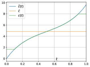
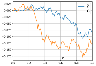
Figure 1: The indifference subscription rate ${\widehat{c}}(t)$, the limiting subscription rate $\overline{c}(t)$, and the prescribed subscription rate $c(t)$.

Figure 2: The signal process $Y_{t}$ and the filtered signal process ${\widehat{Y}}_{t}$.

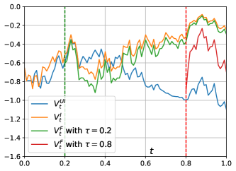
Figure 3: The value functions without information $V_{t}^{UI}$, with information $V_{t}^{I}$ (purchased at time 0 with ${\widehat{C}}(0,T)$) , with prescribed subscription rate $c(t)$ $V_{t}^{F}$.

In this section, we provide an illustrative example of the ideas that we develop. To do so, we make the following model parameter assumptions:

$$\mu=0.05,\;\sigma_{y}=0.1,\;\sigma_{z}=0.05,\;T=1,\;$$

$$\gamma=0.1,\;X_{0}=0,\;Y_{0}=0,\;S_{0}=10.$$

Using these parameters we obtain the indifference subscription rate ${\widehat{c}}$ shown in Figure 3. We further include the limiting subscription rate ${\overline{c}}$ and introduce a prescribed subscription rate $c(t)$ shown in green in the figure. As the prescribed subscription rate lies above the indifference rate prior to $t=0.2=\tau_{e}[c]$, it is never optimal for the investor to subscribe early than $t=0.2$. Similarly, as the prescribed subscription rate lies below the indifference price after $t=0.8=\tau_{\ell}[c]$, it is optimal for the investor to susbcribe no later than $t=0.8$. The investor can subscribe at any time between $\tau_{e}[c]$ and $\tau_{\ell}[c]$ with equal value. In Figure 2, we show a sample path of the true and filtered signals $Y$ and ${\widehat{Y}}$, respectively. In tandem, Figure 3 shows the corresponding sample paths of the value functions without subscribing and with subscribing at different times.

Appendix A Proofs

To ease notation, we define $h(t):=\textstyle\tanh\left(\frac{\sigma_{y}}{\sigma_{z}}t\right)$ and recall that $\ell(t)=\sigma_{y}\sinh(\frac{\sigma_{y}}{\sigma_{z}}(T-2\,t))/4\gamma\,\sigma_{z}\cosh(\frac{\sigma_{y}}{\sigma_{z}}T)$.

A.1 Proof of Theorem 2.1

Proof A.1.

We solve the optimization problem with and without purchasing the information.

Informed case

In the informed case, the investor chooses to purchase the information, hence over $\sigma(Y)$-measurable $\varphi$, she optimizes $\mathbb{E}\left[-\textstyle\exp\left\{-\gamma(x-C+\varphi(Y+Z))\right\}\;|\;\sigma(Y)\right]=-\textstyle\exp\left\{-\gamma(x-C)-\gamma\varphi(Y+\mu)+\frac{1}{2}\gamma^{2}\varphi^{2}\sigma_{Z}^{2}\right\}$ , which yields $\varphi_{I}^{*}=({\mu+Y})/{\gamma\sigma^{2}_{Z}}$ and by the characteristic function of $Y$, we have (4).

Uninformed case

In the uninformed case, the investor does not purchase the information, and hence over deterministic $\varphi\in\mathbb{R}$ she maximizes $\mathbb{E}\left[-\textstyle\exp\left\{-\gamma(x+\varphi(Y+Z))\right\}\right]=\textstyle\exp\left\{-\gamma x-\gamma\varphi(\mu+y)+\frac{1}{2}\gamma^{2}\varphi^{2}\left(\sigma^{2}_{Y}+\sigma_{Z}^{2}\right)\right\}$. Therefore, the (deterministic) optimal strategy is $\varphi_{UI}^{*}={\mu+y}/{\gamma\left(\sigma^{2}_{Y}+\sigma_{Z}^{2}\right)},$ and we have (5).

The investor is indifferent to the two options whenever $V^{I}(x,y;{\widehat{C}})=V^{UI}(x,y)$ and solving for ${\widehat{C}}$ provides us with (6).

A.2 Proof of Lemma 3.1

Proof A.2.

In this proof , we use $L^{2}([0,T]^{2})$ to denote the separable Hilbert spaces of real-valued, square-integrable functions; two functions are considered equal if they coincide almost everywhere. Using Fokker–Planck equation, we can verify that $(S_{t},Y_{t},B^{Z}_{t})$ are jointly Gaussian processes. In particular, $S_{t}-(\mu+y)t-S_{0}$ is a mean zero Gaussian process with covariance function $\mathbb{E}\left[S_{t},S_{u}\right]=\sigma_{z}^{2}u+\sigma_{y}^{2}\left(\frac{t}{2}-\frac{u}{6}\right)u^{2}=\sigma_{z}^{2}u+\sigma_{y}^{2}\textstyle\int_{0}^{t}\int_{0}^{u}\min\{v,s\}dvds$, $\forall\;0\leq u\leq t\leq T$. By checking the conditions in [23, Theorem 1], and by [13, Proposition 2], there exists a unique Brownian motion $(\widehat{B}^{Z}_{t})_{{t\in{\mathfrak{T}}}}$ and a unique kernel $\kappa\in L^{2}([0,T]^{2})$ such that

(22) $$S_{t}=S_{0}+(\mu+y)t+\sigma_{z}\,\widehat{B}^{Z}_{t}-\textstyle\int_{0}^{t}\int_{0}^{u}\kappa(u,v)\,d\widehat{B}^{Z}_{v},\qquad 0\leq t\leq T.$$

Here, the kernel $\kappa$ satisfies the following integral equation:

$$\sigma_{z}\,\kappa(t,u)-\textstyle\int_{0}^{u}\kappa(t,v)\,\kappa(u,v)\,dv=-{\sigma_{y}^{2}}u,\qquad 0\leq u\leq t\leq T,$$

and following similar arguments as in [11, Section 5], $\kappa$ can be calculated explicitly as

(23) $$\kappa(t,u)=-{\sigma_{y}}h(u){{\mathds{1}}_{\{u\in[0,t]\}}}.$$

Recall that for the filtration $\{{\mathcal{F}}_{t}^{S}\}_{{t\in{\mathfrak{T}}}}$ generated by the stock price, we define the projection ${\widehat{Y}}_{t}=\mathbb{E}\left[Y_{t}|{\mathcal{F}}^{S}_{t}\right].$ Hence, by the uniqueness of $(\widehat{B}^{Z}_{t})_{{t\in{\mathfrak{T}}}}$ supported by $\{{\mathcal{F}}_{t}^{S}\}_{{t\in{\mathfrak{T}}}}$, comparison of the dynamic of $S_{t}$ from (7) and (22) yields  (11) and (12) in Lemma 3.1.

A.3 Proof of Theorem 3.2

Proof A.3.

We solve the optimization problem in both the informed and uninformed cases.

Informed Case

In the informed case, at time 0, the investor pays $C(0;T)$ to acquire the full information of $Y_{t}$ on the trading interval $[0,T]$ and, hence, has admissible strategies $\varphi\in{\mathcal{A}}(S,Y)$. The investor’s wealth at time $t$ is thus given by (10), and her goal is to choose $\varphi\in{\mathcal{A}}(S,Y)$ to maximize (9) with $H=1$. The corresponding value function is defined as $V^{I}(t,X_{t},Y_{t};C(0;T)):=\sup_{\varphi\in{\mathcal{A}}(S,Y)}\mathbb{E}\left[-\textstyle\exp\left\{-\gamma X_{T}\right\}|\mathcal{F}_{t}\right]$. Standard arguments suggest that $V^{I}(t,x,y;C(0;T))$ satisfies the HJB equation:

(24) $$\frac{\partial V^{I}}{\partial t}+\frac{1}{2}\sigma_{y}^{2}\frac{\partial^{2}V^{I}}{\partial y^{2}}+\sup_{\varphi}\left\{\frac{1}{2}\sigma_{z}^{2}\varphi^{2}\frac{\partial^{2}V^{I}}{\partial x^{2}}+\varphi(\mu+y)\frac{\partial V^{I}}{\partial x}\right\}=0,$$

with terminal condition $V^{I}(T,x,y;C(0;T))=-\textstyle\exp\left\{-\gamma(x-C(0;T))\right\}$. Point-wise optimization yields the optimal controls in feedback form $\varphi^{I}=-((\mu+y){\partial V^{I}/\partial x})/(\sigma_{z}^{2}{\partial^{2}V^{I}/\partial^{2}x})$. Making the ansatz that $V^{I}(t,x,y;C(0;T))=-\textstyle\exp\left\{-\gamma(x-C(0;T))+A_{I}(t)(\mu+y)^{2}+B_{I}(t)\right\}$, and substituting into the HJB equation (24), we find $(A_{I},B_{I})$ satisfies the following ODEs:

$$\textstyle\tfrac{d}{dt}A_{I}(t)=\frac{1}{2\sigma_{z}^{2}}-2\sigma_{y}^{2}A_{I}(t)^{2}\quad\text{and}\quad\tfrac{d}{dt}B_{I}(t)=-\sigma_{y}^{2}A_{I}(t),$$

with terminal conditions $A_{I}(T)=B_{I}(T)=0$. Solving this system of ODEs, we obtain that

$$\textstyle A_{I}(t)=-\frac{1}{2\sigma_{y}\sigma_{z}}\tanh\left(\frac{\sigma_{y}}{\sigma_{z}}(T-t)\right),\quad B_{I}(t)=-\frac{1}{2}\log\cosh\left(\frac{\sigma_{y}}{\sigma_{z}}(T-t)\right).$$

Accordingly, $\varphi^{I}_{t}=(\mu+Y_{t})/\gamma\sigma_{z}^{2}$, and the value function is (1). By Corollary 5.14 in[14, Chapter 3], the value function is a true martingale.

Uninformed Case

Now let’s assume the investor does not purchase the full information but filters it from $S$. By Lemma 3.1, using the filtered signal process ${\widehat{Y}}$ from (11) and the Brownian motion ${\widehat{B}}$ from (12) under the restricted filtration $\{\mathcal{F}_{t}^{S}\}_{{t\in{\mathfrak{T}}}}$, we can re-write the stock price dynamic as $dS_{t}=(\mu+{\widehat{Y}}_{t})dt+\sigma_{z}d\widehat{B}_{t}^{Z}$. As before, for wealth $X_{t}$ follows (10) with $H=0$, the value function associated with the problem (9) is defined as $V^{UI}(t,X_{t},{\widehat{Y}}_{t}):=\max_{\varphi\in{\mathcal{A}}(S)}\mathbb{E}\left[-\textstyle\exp\left\{-\gamma X_{T}\right\}|\mathcal{F}_{t}^{S}\right].$ From standard analysis, $V^{UI}(t,x,y)$ satisfies the HJB equation (where we write $y$ instead of $\widehat{y}$):

(25) $${\textstyle\frac{\partial V^{UI}}{\partial t}}\!+\!\sup_{\varphi}{\textstyle\Big{\{}\frac{1}{2}\sigma_{z}^{2}\varphi^{2}\frac{\partial^{2}V^{UI}}{\partial x^{2}}+\varphi\left(\sigma_{y}\sigma_{z}h\frac{\partial^{2}V^{UI}}{\partial x\partial y}+(\mu+y)\frac{\partial V^{UI}}{\partial x}\right)\Big{\}}+\frac{1}{2}\sigma_{y}^{2}h^{2}\frac{\partial^{2}V^{UI}}{\partial y^{2}}=0,}$$

subject to the terminal condition $V^{UI}(T,x,y)=-e^{-\gamma x}$. Point-wise optimization provides the optimal controls in feedback form: $\varphi^{UI}=-\textstyle(\sigma_{y}\sigma_{z}h{\partial^{2}V^{UI}}/{\partial x\partial y}+(\mu+y){\partial V^{UI}}/{\partial x})\allowbreak/(\sigma_{z}^{2}\partial^{2}V^{UI}/\partial^{2}x)$. Making a similar ansatz as before $V^{UI}(t,x,y)=-e^{-\gamma x+A_{UI}(t)(\mu+y)^{2}+B_{UI}(t)}$, and substituting into the HJB equation above, we find $(A_{UI},B_{UI})$ satisfies the following ODEs:

$$\textstyle\frac{d}{dt}A_{UI}(t)=\frac{1}{2\sigma_{z}^{2}}+\frac{2\sigma_{y}}{\sigma_{z}}h(t)A_{UI}(t),\quad\text{and}\quad\frac{d}{dt}B_{UI}(t)=-\sigma_{y}^{2}h^{2}(t)A_{UI}(t),$$

subject to $A_{UI}(T)=B_{UI}(T)=0$. Solving the ODEs yields

(26) $$A_{UI}(t) =-\textstyle\frac{\sinh\left(\frac{\sigma_{y}}{\sigma_{z}}(T-t)\right)\cosh\left(\frac{\sigma_{y}}{\sigma_{z}}t\right)}{2\sigma_{y}\sigma_{z}\cosh\left(\frac{\sigma_{y}}{\sigma_{z}}T\right)},$$

(27) $$B_{UI}(t) =\textstyle\frac{\sigma_{y}}{4\sigma_{z}}(T-t)\tanh\left(\frac{\sigma_{y}}{\sigma_{z}}T\right)+\frac{1}{2}\log\frac{\cosh\left(\frac{\sigma_{y}}{\sigma_{z}}t\right)}{\cosh\left(\frac{\sigma_{y}}{\sigma_{z}}T\right)}+\frac{\sinh\left(\frac{\sigma_{y}}{\sigma_{z}}(T-t)\right)\sinh\left(\frac{\sigma_{y}}{\sigma_{z}}t\right)}{4\cosh\left(\frac{\sigma_{y}}{\sigma_{z}}T\right)},$$

and the value function in the uninformed case is therefore (2), with the optimal (filtering) strategy given by the expression stated in Theorem 3.2. By Corollary 5.14 in [14, Chapter 3], the value function is a true martingale.

A.4 Proof of Proposition 4.1

Proof A.4.

First we investigate the value function once information has been purchased. If the investor purchases the information at time ${t\in{\mathfrak{T}}}$, then from the wealth dynamic (18) and a similar procedure to derive the informed value function (1), we have

$$V_{t}^{I}=-\textstyle\exp\left\{-\gamma(X_{t}-\int_{t}^{T}c(s)ds)-\frac{\left(\mu+{Y}_{t}\right)^{2}}{2\sigma_{y}\sigma_{z}}\tanh\left(\frac{\sigma_{y}}{\sigma_{z}}(T-{t})\right)-\frac{1}{2}\log\cosh\left(\frac{\sigma_{y}}{\sigma_{z}}(T-t)\right)\right\}.$$

The expectation ${\widehat{V}}^{I}_{t}$ of the informed value function just prior to acquiring the information is

(28) $${\widehat{V}}^{I}_{t}:=\mathbb{E}\left[V_{t}^{I}|\mathcal{F}^{S}_{t}\right]=V^{UI}_{t}\,\textstyle\exp\Big{\{}\gamma\int_{t}^{T}c(s)ds-B_{UI}(t)+\tfrac{1}{2}\log\frac{\cosh\left(\frac{\sigma_{y}}{\sigma_{z}}t\right)}{\cosh\left(\frac{\sigma_{y}}{\sigma_{z}}T\right)}\Big{\}}.$$

where $V^{UI}_{t}:=V^{UI}(t,X_{t},{\widehat{Y}}_{t})$. The second equality follows from using the value function $V^{UI}$ in (2) and the deterministic function $B_{UI}$ in (27).

Next, we show that $\tau_{\ell}[c]$ in (19) is an upper bound on the time at which the investor is indifferent to purchasing the information feed. To this end, if the investor purchases information at $u\in[t,T]$, then she uses an uninformed strategy on $[t,u]$ (with filtering to obtain ${\widehat{Y}}$) and uses an informed strategy on $[u,T]$ (with knowledge of $Y$). As $(V^{UI}_{t})_{{t\in{\mathfrak{T}}}}$ is a true $\mathcal{F}^{S}$-martingale (by (2)), we have

(29) $$\mathbb{E}[{\widehat{V}}_{u}^{I}|\mathcal{F}^{S}_{t}] =V^{UI}_{t}\;\textstyle\exp\Big{\{}\gamma\int_{u}^{T}c(s)ds-B_{UI}(u)+\frac{1}{2}\log\frac{\cosh\left(\frac{\sigma_{y}}{\sigma_{z}}u\right)}{\cosh\left(\frac{\sigma_{y}}{\sigma_{z}}T\right)}\Big{\}}.$$

The investor will not purchase the information later than $t$ if $\mathbb{E}[{\widehat{V}}_{u}^{I}|\mathcal{F}^{S}_{t}]<{\widehat{V}}_{t}^{I}$, $\forall\;u\in(t,T]$. Comparing (28) and (29) and plugging in the expression for $B_{UI}$ from (27), this means

(30) $$\textstyle\int_{t}^{u}c(s)\,ds <\textstyle\int_{t}^{u}{\overline{c}}-\ell(s)ds.$$

Thus, with ${\overline{c}}$ defined in (16), we introduce the ‘latest subscription time’ $\tau_{\ell}[c]$ of a subscription rate $c$ in (19). If $\tau_{\ell}[c]\in[0,T]$, suppose the investor decides to purchase the information at time $\tau_{0}$, where $\tau_{0}$ is a stopping time in $\mathcal{T}$, we can infer the strict inequality (30) holds if $\tau_{0}>\tau_{\ell}[c]$. Therefore, if $\tau_{0}>\tau_{\ell}[c]$, then $\mathbb{E}\left[{\widehat{V}}_{\tau_{0}}^{I}|\mathcal{F}^{S}_{\tau_{\ell}[c]}\right]<{\widehat{V}}^{I}_{\tau_{\ell}[c]}$, the investor will immediately purchase the information at $\tau_{\ell}[c]$. By the definition of $\tau_{\ell}[c]$, there exists $t\in[0,\tau_{\ell}[c]]$ such that

$$\textstyle\int_{t}^{\tau_{\ell}[c]}\Big{(}c(u)-{\overline{c}}+\ell(s)\Big{)}\,du\geq 0,$$

which makes $\tau_{e}[c]$ given in (20) well defined.

As we have demonstrated that $\tau_{\ell}[c]$ is an upper bound on the optimal stopping time, we focus now on the shortened interval $[0,\tau_{\ell}[c]]$. Let $V^{F}(t,X_{t},{\widehat{Y}}_{t})$ denote the investor’s value function who can choose the purchasing time on $[0,\tau_{\ell}[c]]$ for the information. In the continuation region, $V^{F}$ satisfies

$$\textstyle\sup_{\varphi}\left\{\frac{1}{2}\sigma_{z}^{2}\varphi^{2}\frac{\partial^{2}V^{F}}{\partial x^{2}}+\varphi\left(\sigma_{y}\sigma_{z}h\frac{\partial^{2}V^{F}}{\partial x\partial y}+(\mu+y)\frac{\partial V^{F}}{\partial x}\right)\right\}+\frac{\partial V^{F}}{\partial t}+\frac{1}{2}\sigma_{y}^{2}h^{2}\frac{\partial^{2}V^{F}}{\partial y^{2}}=0,$$

Point-wise optimization yields the optimal controls in feedback form in the continuation region $\varphi^{F}=-(\sigma_{y}\sigma_{z}h{\partial^{2}V^{F}}/{\partial x\partial y}+(\mu+y){\partial V^{F}}/{\partial x})/(\sigma_{z}^{2}\partial^{2}V^{F}/\partial^{2}x).$ Standard arguments imply that $V^{F}$ satisfies the quasi-variational inequality on $[0,\tau_{\ell}[c]]$:

(31) $$\left\{\begin{aligned} &\textstyle\max\Big{\{}\frac{\partial V^{F}}{\partial t}+\frac{\sigma_{y}^{2}}{2}h^{2}\frac{\partial^{2}V^{F}}{\partial y^{2}}-\frac{\left(\frac{\sigma_{y}}{\sigma_{z}}h\frac{\partial^{2}V^{F}}{\partial x\partial y}+\frac{\mu+y}{\sigma_{z}^{2}}\frac{\partial V^{F}}{\partial x}\right)^{2}}{2\frac{\partial^{2}V^{F}}{\partial x^{2}}};{\widehat{V}}^{I}(t,x,y)-V^{F}(t,x,y)\Big{\}}=0\;,\\ &V^{F}(\tau_{\ell}[c],x,y)={\widehat{V}}^{I}(\tau_{\ell}[c],x,y).\end{aligned}\right.$$

When $V^{F}(t,x,y)={\widehat{V}}^{I}(t,x,y)$, it is optimal for the investor to purchase the information. We make the ansatz $V^{F}(t,x,y)=-\textstyle\exp\left\{-\gamma x+A_{UI}(t)(\mu+y)^{2}+B_{F}(t)\right\}$, where $A_{UI}$ is given by (26). Substituting this ansatz into the quasi-variational inequality (31), we obtain a quasi-variational inequality for $B_{F}$ on $[0,\tau_{\ell}[c]]$:

$$\left\{\begin{aligned} &\textstyle\max\Bigg{\{}B_{F}(t)-\textstyle\gamma\int_{t}^{T}c(u)du-\frac{1}{2}\log\frac{\cosh\left(\frac{\sigma_{y}}{\sigma_{z}}t\right)}{\cos\left(\frac{\sigma_{y}}{\sigma_{z}}T\right)}\;;\;\frac{d}{dt}B_{F}(t)+\sigma_{y}^{2}\tanh^{2}\left(\frac{\sigma_{y}}{\sigma_{z}}t\right)A_{UI}(t)\Bigg{\}}=0,\\ &B_{F}(\tau_{\ell}[c])=\gamma\textstyle\int_{\tau_{\ell}[c]}^{T}c(u)du+\frac{1}{2}\log\frac{\cosh\left(\frac{\sigma_{y}}{\sigma_{z}}\tau_{\ell}[c]\right)}{\cos\left(\frac{\sigma_{y}}{\sigma_{z}}T\right)}.\end{aligned}\right.$$

With $A_{UI}$ and ${\widehat{c}}$ given by (26) and (21), respectively, using a comparison argument (cf., e.g., [7]), the unique solution to this variational ODE is

(32) $$B_{F}(t) =\gamma\textstyle\int_{\tau_{\ell}[c]}^{T}c(u)\,du+\gamma\int_{t}^{\tau_{\ell}[c]}{\widehat{c}}(u)\,du+\frac{1}{2}\log\frac{\cosh\left(\frac{\sigma_{y}}{\sigma_{z}}t\right)}{\cosh\left(\frac{\sigma_{y}}{\sigma_{z}}T\right)}.$$

It is optimal for the investor to make the purchase at time $\tau\in[0,\tau_{\ell}[c]]$ whenever $V^{F}(\tau,x,y)={\widehat{V}}^{I}(\tau,x,y)$. Using the above expression and the form of $V^{F}$ and $V^{I}$, $\tau$ is deterministic

(33) $$\textstyle\int_{\tau}^{\tau_{\ell}[c]}(c(s)-{\widehat{c}}(s))\ ds=0.$$

There may be multiple $\tau$ satisfying (33), i.e., at which the investor is indifferent in entering into the subscription. Among them, the earliest time $\tau_{e}[c]$ is given by (20).

We turn to two special cases that demonstrate that $\tau_{e}[c]$ and $\tau_{\ell}[c]$ are not necessarily equal.

Special case with ${\overline{c}}$ by (16)

In this case, as $\sinh(x)$ is strictly positive on $(0,\infty)$ and strictly negative on $(-\infty,0)$, we have that

$$\tau_{\ell}[{\overline{c}}]=\textstyle\inf\left\{{t\in{\mathfrak{T}}}:\int_{t}^{u}\ell(s)ds<0,\forall u\in(t,T]\right\}=\frac{T}{2}.$$

Notice that for $t\in[0,\tau_{\ell}[{\overline{c}}])$, $\textstyle\int_{t}^{\tau_{\ell}[{\overline{c}}]}\ell(s)\;ds>0$. Hence for the limiting subscription rate ${\overline{c}}$ in (16), the investor purchases the information subscription at time $\tau_{e}[{\overline{c}}]={T}/{2}=\tau_{\ell}[{\overline{c}}]$.

Special case with ${\widehat{c}}(t)$ by (21)

In this case, the term under the integral in the expression for $\tau_{\ell}[{\widehat{c}}]$ is identically zero, hence $\textstyle\left\{t\in{\mathfrak{T}}:0<0,\forall u\in(t,T]\right\}=\emptyset$. By definition, we have $\tau_{\ell}[{\widehat{c}}]=T$. Moreover, on $[0,T]$ we have that

$$\textstyle\int_{t}^{T}({\widehat{c}}(s)-{\widehat{c}}(s))\ ds=0,\quad\mbox{for all}\;t\in[0,T],$$

and, therefore, the investor is indifferent between purchasing the information subscription or trading with the information of the stock over the whole time period, hence the earliest time to make the purchase is therefore $\tau_{e}[{\widehat{c}}]=0\neq\tau_{\ell}[{\widehat{c}}]=T$.

References

• [1] A. Al-Aradi and S. Jaimungal, Outperformance and tracking: Dynamic asset allocation for active and passive portfolio management, Applied Mathematical Finance, 25 (2018), pp. 268–294.
• [2] J. Amendinger, P. Imkeller, and M. Schweizer, Additional logarithmic utility of an insider, Stochastic processes and their applications, 75 (1998), pp. 263–286.
• [3] S. Banerjee and B. Breon-Drish, Strategic trading and unobservable information acquisition, Journal of Financial Economics, 138 (2020), pp. 458–482.
• [4] V. E. Beneš and I. Karatzas, Estimation and control for linear, partially observable systems with non-gaussian initial distribution, Stochastic Processes and their Applications, 14 (1983), pp. 233–248.
• [5] S. Brendle, Portfolio selection under incomplete information, Stochastic processes and their Applications, 116 (2006), pp. 701–723.
• [6] P. Casgrain and S. Jaimungal, Trading algorithms with learning in latent alpha models, Mathematical Finance, 29 (2019), pp. 735–772.
• [7] C. Chicone, Ordinary differential equations with applications, vol. 34, Springer Science & Business Media, 2006.
• [8] J. Cvitanić, A. Lazrak, L. Martellini, and F. Zapatero, Dynamic portfolio choice with parameter uncertainty and the economic value of analysts’ recommendations, The Review of Financial Studies, 19 (2006), pp. 1113–1156.
• [9] J. B. Detemple, Asset pricing in a production economy with incomplete information, The Journal of Finance, 41 (1986), pp. 383–391.
• [10] J.-P. Fouque, A. Papanicolaou, and R. Sircar, Filtering and portfolio optimization with stochastic unobserved drift in asset returns, Communications in Mathematical Sciences, 13 (2015), pp. 935–953.
• [11] P. Guasoni, Asymmetric information in fads models, Finance and Stochastics, 10 (2006), pp. 159–177.
• [12] P. Guasoni, A. Tolomeo, and G. Wang, Should commodity investors follow commodities’ prices?, SIAM Journal on Financial Mathematics, 10 (2019), pp. 466–490.
• [13] M. Hitsuda, Representation of Gaussian processes equivalent to Wiener process, Osaka J. Math., (1968).
• [14] I. Karatzas and S. Shreve, Brownian motion and stochastic calculus, vol. 113, Springer Science & Business Media, 2012.
• [15] T. S. Kim and E. Omberg, Dynamic nonmyopic portfolio behavior, The Review of Financial Studies, 9 (1996), pp. 141–161.
• [16] A. S. Kyle, Continuous auctions and insider trading, Econometrica, 53 (1985), pp. 1315–1335.
• [17] M. Ludkovski, A simulation approach to optimal stopping under partial information, Stochastic processes and their applications, 119 (2009), pp. 4061–4087.
• [18] M. Ludkovski and S. O. Sezer, Finite horizon decision timing with partially observable poisson processes, Stochastic Models, 28 (2012), pp. 207–247.
• [19] R. C. Merton, Optimum consumption and portfolio rules in a continuous-time model, in Stochastic optimization models in finance, Elsevier, 1975, pp. 621–661.
• [20] A. Papanicolaou, Backward sdes for control with partial information, Mathematical Finance, 29 (2019), pp. 208–248.
• [21] I. Pikovsky and I. Karatzas, Anticipative portfolio optimization, Advances in Applied Probability, 28 (1996), pp. 1095–1122.
• [22] U. Rieder and N. Bäuerle, Portfolio optimization with unobservable markov-modulated drift process, Journal of Applied Probability, 42 (2005), pp. 362–378.
• [23] L. A. Shepp, Radon-nikodym derivatives of gaussian measures, The Annals of Mathematical Statistics, (1966), pp. 321–354.
• [24] Y. Xia, Learning about predictability: The effects of parameter uncertainty on dynamic asset allocation, The Journal of Finance, 56 (2001), pp. 205–246.
• [25] J. Yang, L. Zhang, N. Chen, R. Gao, and M. Hu, Decision-making with side information: A causal transport robust approach.