UniST: A Prompt-Empowered Universal Model for Urban Spatio-Temporal Prediction

Abstract.

Urban spatio-temporal prediction is crucial for informed decision-making, such as transportation management, resource optimization, and urban planning. Although pretrained foundation models for natural languages have experienced remarkable breakthroughs, wherein one general-purpose model can tackle multiple tasks across various domains, urban spatio-temporal modeling lags behind. Existing approaches for urban prediction are usually tailored for specific spatio-temporal scenarios, requiring task-specific model designs and extensive in-domain training data. In this work, we propose a universal model, UniST, for urban spatio-temporal prediction. Drawing inspiration from large language models, UniST achieves success through: (i) flexibility towards diverse spatio-temporal data characteristics, (ii) effective generative pre-training with elaborated masking strategies to capture complex spatio-temporal relationships, (iii) spatio-temporal knowledge-guided prompts that align and leverage intrinsic and shared knowledge across scenarios. These designs together unlock the potential of a one-for-all model for spatio-temporal prediction with powerful generalization capability. Extensive experiments on 15 cities and 6 domains demonstrate the universality of UniST in advancing state-of-the-art prediction performance, especially in few-shot and zero-shot scenarios.

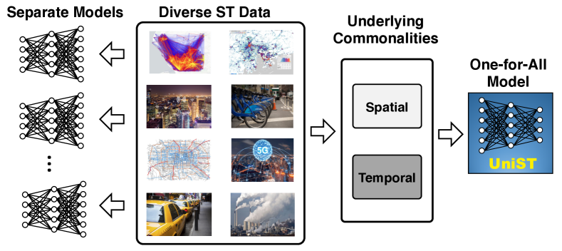
Figure 1. From traditional separate deep models to a one-for-all universal model for urban spatio-temporal prediction.

1. Introduction

Pre-trained foundation models have showcased remarkable success in Natural Language Processing (NLP) (Touvron et al., 2023, 2023; Brown et al., 2020), particularly excelling in few-shot and zero-shot scenarios (Brown et al., 2020; Kojima et al., 2022). However, the field of urban spatio-temporal modeling (Wang et al., 2020; Zheng et al., 2014; Jin et al., 2023b) has not witnessed a parallel breakthrough. In this paper, our goal is to build a foundation model for urban spatio-temporal prediction, that is, to develop a universal spatio-temporal model, i.e., a one-for-all model, with superior performance and robust generalization capability across diverse spatio-temporal scenarios. These scenarios encompass a wide range of domains, such as transportation, cellular network, and human mobility, spanning various cities.

The significance of such a universal model lies in its ability to address prevalent data scarcity issues in urban areas, where varying degrees of digitization result in imbalanced data collections across different cities and domains. While impressive progress has been made in existing spatio-temporal modeling approaches (Bai et al., 2020; Zhang et al., 2017; Liu et al., 2018; Cheng et al., 2023; Bai et al., 2019a; Zhou et al., 2023b; Xia et al., 2023; Liang et al., 2018, 2019; Pan et al., 2019, 2020; Liang et al., 2021b, a; Zhou et al., 2023d), their effectiveness is often constrained by rigid specialization to a particular domain in one city, i.e., a specific dataset. The reliance on extensive training data further impedes the model’s generalization potential. Consequently, current solutions are still far from “universality”, and have restrictive applications.

A universal spatio-temporal model should have the following two capabilities. Firstly, it must be capable of leveraging abundant and rich data from urban scenarios for training, particularly data characterized by varying spatio-temporal features. The training of the foundational model should ensure the acquisition of ample and rich information (Touvron et al., 2023; Wang et al., 2023; Bai et al., 2023). Second, it should demonstrate robust generalization across diverse spatio-temporal scenarios. Especially in scenarios with limited or no training data, the model can still predict well without much performance degradation (Garza and Mergenthaler-Canseco, 2023; Kirillov et al., 2023; Wang et al., 2023). Crucially, this capability emerges not only from diverse data training, but also from the shared and transferable knowledge across scenarios.

However, realizing the aforementioned two characteristics is technically non-trivial. Several challenges unique to spatio-temporal data prevent the direct adoption of current foundation models from the language or vision domains. The first challenge arises from diverse data formats inherent in spatio-temporal datasets. Unlike languages with a natural and unified 1D structure or images and videos adhering to standard formats, spatio-temporal data collected from different sources exhibit completely different features. The variable dimension, temporal duration, and spatial range may vary significantly, making it difficult to impose a standardized structure. The second challenge arises from the high variations in data distributions across multiple scenarios. Faced with highly distinct spatio-temporal patterns, the model may struggle to adapt to these differences. Moreover, unlike NLP, which benefits from a shared vocabulary, different spatio-temporal scenarios often have entirely different spatial and temporal scales, lacking common elements for knowledge sharing and transfer.

Although the displayed spatio-temporal patterns vary significantly, we believe that some underlying principles are shared among these diverse scenarios. For instance, the locations of commercial centers in different cities are probably different, yet the way they correlate with other functional districts could be a shared characteristic. Similarly, while temporal periodic patterns differ across domains, they share the essential concept of repetitive patterns. Therefore, the key point of building a one-for-all model is to align and leverage these shared but underlying characteristics.

We propose UniST, a universal solution for urban spatio-temporal prediction. Notably, it ingeniously imitates the key features of LLMs:

1. Flexibility towards diverse data characteristics;

2. Effective pre-training to capture multi-level spatio-temporal relationships;

3. Spatio-temporal knowledge-guided prompt to align underlying and shared commonalities across scenarios.

UniST achieves the above characteristics through its holistic design, which is specified by four key components: data, architecture, pre-training, and prompt tuning. Firstly, we seek to harness the rich diversity inherent in spatio-temporal scenarios by collecting extensive data from various cities and domains. Secondly, we employ spatio-temporal tokenizers to convert diverse data shapes into a unified sequential format, which facilities to utilize the powerful Transformer architecture. Thirdly, drawing inspiration from language (Devlin et al., 2018; Brown et al., 2020) and vision communities (He et al., 2022), UniST adopts the widely-used generative pre-training strategy – masked token modeling. Going beyond, we employ different masking strategies tailored for spatio-temporal data, refining the model’s ability to comprehensively capture spatio-temporal correlations. Moreover, we introduce an innovative spatio-temporal knowledge-guided prompt mechanism. Inspired by well-established domain knowledge in spatio-temporal modeling, an elaborated prompt network identifies underlying and shared spatio-temporal properties, and learns to adaptively leverage them to generate useful prompts. In this way, we can align distinct data distributions of various datasets and develop a one-for-all universal model. We summarize our contributions as follows:

• To the best of our knowledge, this is the first attempt to address the universal spatio-temporal prediction, which investigates the potential of a one-for-all model in diverse urban scenarios.

• We propose UniST, a universal spatio-temporal prediction model. Through the elaborated masking strategies and spatio-temporal knowledge-guided prompts, it manages to harness the data diversity and achieve a universal solution for all scenarios. It represents a paradigm shift in spatio-temporal prediction from traditional separate methods to pre-trained foundational models.

• Extensive experiments demonstrate the strong universality of UniST. It achieves new state-of-the-art performance on various prediction tasks. Particularly, it demonstrates superior transferability to previously unseen scenarios.

2. Related Work

Urban Spatio-Temporal Prediction.

Urban spatio-temporal prediction (Wang et al., 2020; Zheng et al., 2014; Jin et al., 2023b) aims to model and forecast the dynamic patterns of urban activities over both space and time. The advent of deep learning techniques has propelled significant advancements in urban spatio-temporal prediction. A spectrum of models, including CNN-based (Li et al., 2018; Zhang et al., 2017; Liu et al., 2018), RNN-based (Wang et al., 2017, 2018a; Lin et al., 2020; Bai et al., 2019c), ResNet-based (Zhang et al., 2017), GNN-based (Zhao et al., 2019; Jin et al., 2023b; Bai et al., 2020, 2019a, 2019b; Geng et al., 2019), Transformer-based (Chen et al., 2022; Jiang et al., 2023a; Yu et al., 2020; Chen et al., 2021), MLP-based (Zhang et al., 2023c; Shao et al., 2022) and diffusion model-based (Zhou et al., 2023a; Wen et al., 2023; Yuan et al., 2023) architectures, has been proposed to capture spatio-temporal relationships. Simultaneously, cutting-edge learning techniques like meta-learning (Chen et al., 2023; Pan et al., 2020; Lu et al., 2022; Yao et al., 2019), contrastive learning (Ji et al., 2023; Liu et al., 2022; Zhang et al., 2023b; Tang et al., 2023), and adversarial learning (Ouyang et al., 2023; Gao et al., 2022b; Fang et al., 2022; Tang et al., 2022) are also utilized. However, most existing approaches remain constrained by training separate models for each specific domain. Some studies (Yao et al., 2019; Lu et al., 2022; Jin et al., 2022; Wang et al., 2018b; Jin et al., 2023a; Jiang et al., 2023b; Liu et al., 2023e; Chen et al., 2023; Fang et al., 2022) explore transfer learning between cities, however, a certain amount of data samples in the target city are still required. Current solutions are restrictive to specified domains or cities that have training data. On the contrary, our model allows training and predicting across diverse spatio-temporal scenarios and provides a universal solution.

Foundation Models for Spatio-temporal Data and Time Series.

Inspired by the remarkable strides in foundation models for NLP (Touvron et al., 2023, 2023; Brown et al., 2020) and CV (Rombach et al., 2022; Bai et al., 2023), the exploration of foundation models for urban scenarios has emerged as a compelling problem. Current explorations mainly unlock the potential of LLMs in this context. State-of-the-art urban systems like TransGPT (Tra, 2023), CityGPT (Xu et al., 2023), and TrafficGPT (Zhang et al., 2023a; Da et al., 2023) have demonstrated proficiency in addressing language-based spatio-temporal tasks. Additionally, LLMs are utilized to articulate descriptions for urban-related images (Yan et al., 2023), which is useful for downstream tasks. Moreover, the application of LLMs extends to traffic signal control (Lai et al., 2023), showcasing their utility in tackling complex spatio-temporal problems beyond languages. Recently, there has been great progress in foundation models for time series modeling (Jin et al., 2023d; Cao et al., 2023; Jin et al., 2023c; Liu et al., 2023a; Zhou et al., 2023c). Unlike time series characterized by a straightforward 1D structure, spatio-temporal data presents a more intricate nature with intertwined dependencies across both spatial and temporal dimensions. We think that spatio-temporal data is not inherently reliant on language. While the integration of LLMs is both interesting and worthy of exploration, developing a foundation model that specifically goes from spatio-temporal data, also holds significant importance.

Prompt Tuning Techniques

Prompting techniques have achieved superior performance in Natural Language Processing (NLP) (Liu et al., 2023d; Qiao et al., 2022) and Computer Vision (CV) (Jia et al., 2022; Shen et al., 2024) fields. The goal is to enhance the generalization capability of pretrained models on specific tasks or domains. Typically, language models usually use a limited number of demonstrations as prompts and vision models often employ a learnable prompt network to generate useful prompts, known as prompt tuning. Our research aligns with prompt tuning, where spatio-temporal prompts are adaptively generated based on the spatio-temporal properties through a prompt network.

3. Preliminary

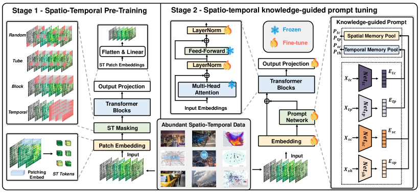
Figure 2. The overview of UniST, which consists of two stages: (i) large-scale spatio-temporal pre-trianing, (ii) spatio-temporal knowledge-guided prompt tuning.

Spatial Partition and Temporal Aggregation.

The spatial partition and temporal aggregation vary across different spatio-temporal scenarios. In this study, we focus on grid-based spatial partitioning, where the spatial dimension is discretized into non-overlapping grids of equal size based on longitude and latitude. The grid map takes the form of an $H\times W$ rectangle, with each grid representing a distinct geographical region within the city. Temporal aggregation involves collecting data over specific temporal intervals. For example, crowd flows are documented on an hourly basis, while bike usage data is logged every half an hour.

Spatio-temporal Data.

With the spatial partition and temporal aggregation described above, spatio-temporal data in our study can be defined as a four-dimensional tensor: $T\times C\times H\times W$, where $T$ represents the number of time periods, $H$ and $W$ represent the number of grids in the longitude and latitude dimensions of the spatial partition, respectively, and $C$ represents the number of variables. Notably, $T$, $C$, $H$, and $W$ often vary across scenarios due to different sensors and implementations driven by specific objectives.

Spatio-temporal Prediction.

For a specific dataset, given $L_{H}$ historical observations $X$ for the grid map, we aim to predict the future $k$ steps. The spatio-temporal prediction task can be formulated as learning a $\theta$-parameterized model $\mathcal{F}$: $X_{[t:t+k]}=\mathcal{F}_{\theta}(X_{[t-L_{H}:t]})$.

Spatio-temporal Few-shot Prediction.

Consider a collection of source datasets denoted as ${X^{1},X^{2},...,X^{N}}$, and a target dataset $X^{tar}$ characterized by limited data. After training a model on the source datasets, the model can leverage acquired knowledge to adapt to the target dataset, even with limited training data.

Spatio-temproal Zero-shot Prediction.

The model can directly predict without additional training on the target dataset.

4. The UniST Model

We propose the UniST model to address universal spatio-temporal prediction, which is shown in Figure 2. It consists of two stages:

• Stage 1: Large-scale spatio-temporal pre-training. Different from existing methods limited to a single dataset, our approach involves collecting extensive spatio-temporal data from a variety of cities and domains for pre-training. Concurrently, we introduce innovative spatio-temporal masking and reconstruction strategies to further enhance the pre-training process.

• Stage 2: Spatio-temporal knowledge-guided prompt tuning. This stage introduces a prompt network for in-context learning. The generation of prompts is adaptively guided by well-developed spatio-temporal domain knowledge. We fix the feed-forward and attention layers of the base Transformer model. Subsequently, we fine-tune both the prompt network and the remaining parameters of the Transformer model.

4.1. Base Model

The base model is a Transformer-based encoder-decoder architecture. Through spatio-temporal tokenizers, the base model can deal with diverse spatio-temporal data in a unified sequential format.

4.1.1. Spatio-temporal Tokenizers

The conventional Transformer architecture is designed for processing 1D sequential data. However, spatio-temporal data possesses a 4D structure. To accommodate this, we first split the data into channel-independent instances, which are 3D tensors. Then, we utilize spatio-temporal tokenizers to transform the 3D tensor, denoted as $X\in\mathbb{R}^{L\times H\times W}$, into multiple smaller 3D tensors. If the original shape is $L\times H\times W$, and the patch size is $(l,h,w)$, the resulting sequence is given by $E_{x}\in\mathbb{R}^{L^{\prime}\times H^{\prime}\times W^{\prime}},L^{\prime}=\frac{L}{l},H^{\prime}=\frac{H}{h},W^{\prime}=\frac{W}{w}$.

This transformation involves a 3D convolutional layer with a kernel size and stride both set to $(l,h,w)$. The process can be expressed as $E_{x}=\text{Conv}_{3d}(X))$, where $E_{x}$ represents the converted 1D sequential data. The sequence length of $E_{x}$ is $L^{\prime}\times H^{\prime}\times W^{\prime}$.

4.1.2. Positional Encoding.

As the original Transformer architecture does not consider the order of the sequence, we follow the common practice (Devlin et al., 2018) that incorporate positional encoding. To enhance generalization, we choose sine and cosine functions rather than learnable parameters for positional encoding. This encoding is separately applied to the spatial and temporal dimensions.

4.1.3. Encoder-decoder Structure

The base model adopts an encoder-decoder structure, following the methodology in Masked Autoencoder (MAE) (He et al., 2022). Input patches undergo masking at a certain ratio, and subsequently, the encoder receives the unmasked patches. Then, the decoder receives the encoder output and the masked patches and performs the reconstruction. However, our primary focus lies in capturing spatio-temporal dependencies encompassing both high-level and low-level relationships. For instance, we aim to predict precise values at specific grids in both time and space. Thus, we employ a decoder of comparable size to the encoder, different from the lightweight decoder used in MAE. Unlike the MAE decoder, exclusively utilized in the pre-training phase for image reconstruction, our decoder plays a pivotal role in both the pre-training and fine-tuning stages. The encoder and the decoder can be formulated as follows:

(1) $$E_{enc}=\text{Encoder}(E_{x}),\ Y_{dec}=\text{Decoder}(E_{enc},E_{mask}),$$

where $E_{mask}$ denotes the token embeddings for the masked patch.

4.2. Spatio-temporal Self-supervised Pretraining

In pretrained language models, the self-supervised learning task is either masking-reconstruction (Devlin et al., 2018) or autoregressive prediction (Brown et al., 2020). Similarly, in vision models, visual patches are randomly masked and the pretraining objective is to reconstruct the masked pixels. To further augment the model’s capacity to capture intricate spatio-temporal relationships and intertwined dynamics, we introduce four distinct masking strategies during the pretraining phase, which are shown in the left box in the stage 1 of Figure 2. Suppose the masking percentage is $r$, we explain these strategies as follows:

• Random masking. This strategy is similar to the one used in MAE, where spatio-temporal patches are randomly masked. Its purpose is to capture fine-grained spatio-temporal relationships.

  (2) $$M\sim\textbf{U}[0,1],\ E_{x}=E_{x}[M<1-r],\ M\in\mathbb{R}^{L^{\prime}\times H^{\prime}\times W^{\prime}}.$$

• Tube masking. This strategy simulates scenarios where data for certain spatial units is entirely missing across all instances in time, mirroring real-world situations where some sensors may be nonfunctional—a common occurrence. The goal is to improve spatial extrapolation competence.

  (3) $$M\sim\textbf{U}[0,1],\ E_{x}=E_{x}[\ :\ ,M<1-r],\ M\in\mathbb{R}^{H^{\prime}\times W^{\prime}}.$$

• Block masking. A more challenging variant of tube masking, block masking involves the complete absence of an entire block of spatial units across all instances in time. The reconstruction task becomes more intricate due to limited context information, with the objective of enhancing spatial transferability.

  (4) $$M\sim\textbf{Uniform}(1,2),\ E_{x}=E_{x}[\ :\ ,\frac{M-1}{2}H^{\prime}:\frac{M}{2}H^{\prime}].$$

• Temporal Masking. In this approach, future data is masked, compelling the model to reconstruct the future based solely on historical information. The aim is to refine the model’s capability to capture temporal dependencies from the past to the future.

  (5) $$M=\text{Concat}([\textbf{1}_{(1-r)L^{\prime}\times H^{\prime}\times W^{\prime}},\textbf{0}_{rL^{\prime}\times H^{\prime}\times W^{\prime}}]),\ E_{x}=E_{x}[M=1].$$

By employing these diverse masking strategies, the model can systematically enhance its modeling capabilities from a comprehensive perspective, simultaneously addressing spatio-temporal, spatial, and temporal relationships.

4.3. Spatio-temporal Knowledge-Guided Prompt

Prompt tuning plays a critical role in enhancing UniST’s generalization ability. Before delving into the details of our prompt design, it is essential to discuss why pre-trained models can be applied to unseen tasks and domains.

4.3.1. Spatial-Temporal Generalization.

In urban areas, the distributions of features and labels differ across cities and domains, denoted as $X_{A}\neq X_{B},Y_{A}\neq Y_{B}$, where $X$ and $Y$ denote features and labels, while $A$ and $B$ represent different cities or domains. Taken $A$ and $B$ as a simple example, generalization involves leveraging knowledge acquired from the $A$ dataset and adapt it to the $B$ dataset. The key point lies in identifying and aligning “related” patterns between $A$ and $B$ datasets. While finding similar patterns for an entire dataset may be challenging, we claim that identifying and aligning fine-grained patterns is feasible. Specifically, we provide some assumptions that applies to prompt-empowered spatio-temporal generalization, which are expressed as follows:

Assumption 1.

For a new dataset $\bf{B}$, it is possible to identify fine-grained patterns related to the training data $\bf{A}$.

(6) $$X_{A}\neq X_{B},\ Y_{A}\neq Y_{B},$$

$$\exists x_{a}\in X_{A},y_{a}\in Y_{A},\ \exists x_{b}\in X_{B},y_{b}\in Y_{B},:x_{a}\approx x_{b},y_{a}\approx y_{b}.$$

Assumption 2.

Distinct spatio-temporal patterns correspond to customized prompts.

(7) $$P_{i}^{*}\neq P_{j}^{*}\quad\text{if}\quad D(x_{i},x_{j})>\epsilon,$$

$$D(P_{i}^{*},P_{j}^{*})>D(P_{m}^{*},P_{n}^{*})\quad\text{if}\quad D(x_{i},x_{j})>D(x_{m},x_{n}),$$

where $x_{i}$ denotes the fine-grained spatio-temporal pattern, $P_{i}^{*}$ represents the prompt of $x_{i}$, and $D$ is the similarity between $x_{i}$ and $x_{j}$.

Assumption 3.

There exists $f_{\theta}$ that captures the mapping relationship from the spatio-temporal pattern $x_{i}$ to prompt $P_{i}^{*}$.

$$P_{i}=f_{\theta}(x_{i})\quad\text{where}\quad\theta=\underset{\theta}{\text{argmin}}\sum_{i}\text{Distance}(P_{i}^{*},f_{\theta}(x_{i})).$$

Based on these assumptions, our core idea is that for different inputs with distinct spatio-temporal patterns, customized prompts should be generated adaptively.

4.3.2. Spatio-Temporal Domain Knowledge

Given the aforementioned assumptions, a critical consideration is how to define the concept of “similarity” to identify and align shared spatio-temporal patterns. Here we leverage insights from well-established domain knowledge in spatio-temporal modeling (Zheng et al., 2014; Zhang et al., 2017), encompassing properties related to both space and time. There are four aspects to consider when examining these properties:

• Spatial closeness: Nearby units may influence each other.

• Spatial hierarchy: The spatial hierarchical organization impacts the spatio-temporal dynamics, requiring a multi-level perception on the city structure.

• Temporal closeness: Recent dynamics affect future results, indicating a closeness dependence.

• Temporal period: Daily or weekly patterns exhibit similarities, displaying a certain periodicity.

For simplicity, we provide some straightforward implementations, which are shown in the four networks in Figure 2, i.e., $Net_{tc}$, $Net_{tp}$, $Net_{sc}$, and $Net_{sh}$. For the spatial dimension, we first employ an attention mechanism to merge the temporal dimension into a representation termed $E_{s}$. Then, to capture spatial dependencies within close proximity, a 2D convolutional neural network (CNN), i.e., $Net_{sc}$, with a kernel size of 3 is employed. To capture spatial hierarchies, we utilize CNNs with larger kernel sizes, i.e., $Net_{sh}$. These larger kernels enable the perception of spatial information on larger scales, which facilitate to construct a hierarchical perspective. As for the temporal dimension, we employ an attention network, i.e., $Net_{tc}$, to aggregate the previous M steps denoted as $X_{c}$. Regarding the temporal period, we select corresponding time points from the previous N days, denoted as $X_{p}$. Subsequently, we employ another attention network, i.e., $Net_{tp}$, to aggregate the periodical sequence, which captures long-term temporal patterns. The overall process is formulated as follows:

(8) $$E_{sc}=\text{Conv}_{2D}[3](X_{s}),E_{sh}=\{\text{Conv}_{2D}[2^{i}+1](X_{s})\},i\in\{2,3,4\},$$

(9) $$E_{tc}=\text{Attention}_{t}(X_{c}),E_{tp}=\text{Attention}_{p}(X_{p}).$$

It is essential to emphasize that the learning of $E_{sc},E_{sh},E_{tc}$, and $E_{tp}$ is not restricted by our practice. Practitioners have the flexibility to employ more complex designs to capture richer spatio-temporal properties. For example, Fourier-based approaches (Wu et al., 2022; Liu et al., 2023c) can be utilized to capture periodic patterns.

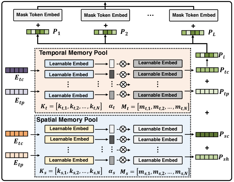
Figure 3. Illustration of the prompt generation process.

4.3.3. Spatio-temporal Prompt Learner

Given the representations of properties derived from spatio-temporal domain knowledge, the pivotal question is how to generate prompts—how does spatio-temporal knowledge guide prompt generation? Here we utilize prompt tuning techniques. While prompt tuning in computer vision (Jia et al., 2022) often train fixed prompts for specific tasks such as segmentation, detection, and classification. Due to the high-dimensional and complex nature of spatio-temporal patterns, training a fixed prompt for each case becomes impractical.

To tackle this issue, we draw inspirations from memory networks (Sukhbaatar et al., 2015) and propose a novel approach that learns a spatial memory pool and a temporal memory pool. In the prompt tuning process, these memory pools are optimized to store valuable information about spatio-temporal domain knowledge. As shown in Figure 3, the spatial and memory pools are defined as follows:

(10) $$KM_{s}=\{(k_{s,0},m_{s,0}),(k_{s,1},m_{s,1}),...,(k_{s,N-1},m_{s,N-1})\},$$

$$KM_{t}=\{(k_{t,0},m_{t,0}),(k_{t,1},m_{t,1}),...,(k_{t,N-1},m_{t,N-1})\},$$

where $k_{s,i},m_{s,i},k_{t,i},m_{t,i},i\in\{0,1,...,N-1\}$ are all learnable parameters, and the memory is organized in a key-value structure following existing practice (Sukhbaatar et al., 2015; Wang et al., 2022).

Subsequently, useful prompts are generated based on these optimized memories. This involves using the representations of spatio-temporal properties as queries to extract valuable memory knowledge, i.e., pertinent embeddings from the memory pool. Figure 3 illustrates the process, and it is formulated as follows:

(11) $$\alpha_{sc}=[k_{s,0};k_{s,1};...,k_{s,N-1}]E_{sc}^{T},\ P_{sc}=\sum_{i}\alpha_{sc,i}m_{s,i},$$

$$\alpha_{sh}=[k_{s,0};k_{s,1};...,k_{s,N-1}]E_{sh}^{T},\ P_{sh}=\sum_{i}\alpha_{sh,i}m_{s,i},$$

$$\alpha_{tc}=[k_{t,0};k_{t,1};...,k_{t,N-1}]E_{tc}^{T},\ P_{tc}=\sum_{i}\alpha_{tc,i}m_{t,i},$$

$$\alpha_{tp}=[k_{t,0};k_{t,1};...,k_{t,N-1}]E_{tp}^{T},\ P_{tp}=\sum_{i}\alpha_{tp,i}m_{t,i},$$

where $E_{sc},E_{sh},E_{tc},E_{tp}$ represent four representations related to four types of spatio-temporal domain knowledge, and $P_{sc},P_{sh},P_{tc},P_{tp}$ are the extracted prompts. This allows the model to adaptively select the most useful information for prediction. These prompts are then integrated into the input space of the Transformer architecture, which are displayed in the upper part of Figure 3.

Table 1. Performance comparison of short-term prediction on seven datasets in terms of MAE and RMSE. We use the average prediction errors overall prediction steps. Bold denotes the best results and underline denotes the second-best results.

	TaxiBJ		Crowd		Cellular		BikeNYC		TrafficJN		TDrive		TrafficSH
Model	RMSE	MAE	RMSE	MAE	RMSE	MAE	RMSE	MAE	RMSE	MAE	RMSE	MAE	RMSE	MAE
HA	53.77	29.82	17.80	6.79	72.94	27.57	11.41	3.43	1.38	0.690	150.2	74.5	1.24	0.771
ARIMA	56.70	39.53	21.87	10.23	81.31	40.22	12.37	3.86	1.20	0.651	211.3	108.5	1.17	0.769
STResNet	45.17	30.87	5.355	3.382	24.30	14.32	8.20	4.98	0.964	0.556	220.1	117.4	1.00	0.723
ACFM	37.77	21.59	4.17	2.34	22.79	12.00	3.93	1.67	0.920	0.559	98.1	51.9	0.833	0.566
STID	27.36	14.01	3.85	1.63	18.77	8.24	4.06	1.54	0.880	0.495	47.4	23.3	0.742	0.469
STNorm	29.37	15.71	4.44	2.09	19.77	8.19	4.45	1.66	0.961	0.532	54.3	47.9	0.871	0.579
STGSP	45.04	28.28	7.93	4.56	39.99	21.40	5.00	1.69	0.882	0.490	94.6	47.8	1.02	0.749
MC-STL	29.14	15.83	4.75	2.39	21.22	10.26	4.08	2.05	1.19	0.833	54.2	28.1	1.00	0.720
MAU	38.14	20.13	4.94	2.35	39.09	18.73	5.22	2.06	1.28	0.697	48.8	22.1	1.37	0.991
PredRNN	27.50	14.29	5.13	2.36	24.15	10.44	5.00	1.74	0.852	0.463	54.9	25.2	0.748	0.469
MIM	28.62	14.77	5.66	2.27	21.38	9.37	4.40	1.62	1.17	0.650	51.4	22.7	0.760	0.505
SimVP	32.66	17.67	3.91	1.96	16.48	8.23	4.11	1.67	0.969	0.556	46.8	22.9	0.814	0.569
TAU	33.90	19.37	4.09	2.11	17.94	8.91	4.30	1.83	0.993	0.566	51.6	28.1	0.820	0.557
PatchTST	42.74	22.23	10.25	3.62	43.40	15.74	5.27	1.65	1.25	0.616	106.4	51.3	1.10	0.663
iTransformer	36.97	19.14	9.40	3.40	37.01	13.93	7.74	2.53	1.11	0.570	86.3	42.6	1.04	0.655
PatchTST(one-for-all)	43.66	23.16	13.51	5.00	56.80	20.56	9.97	3.05	1.30	0.645	127.0	59.26	1.13	0.679
UniST(one-for-all)	26.84	13.95	3.00	1.38	14.29	6.50	3.50	1.27	0.843	0.430	44.97	19.67	0.665	0.405
Reduction	1.9%	0.42%	22.0%	15.7%	13.2%	20.6%	10.9%	21.6%	1.1%	7.1%	4.1%	13.3%	10.3%	13.6%

5. Results

5.1. Experimental Setup

To evaluate the performance of UniST, we conducted extensive experiments on more than 20 spatio-temporal datasets.

Datasets. The datasets we used cover multiple cities, spanning various domains such as crowd flow, dynamic population, traffic speed, cellular network usage, taxi trips, and bike demand. Appendix A Table 3 and Table 4 provide a summary of the datasets we used. These spatio-temporal datasets originate from distinct domains and cities, and have variations in the number of variables, sampling frequency, spatial scale, temporal duration, and data size.

Baselines. We compare UniST with a broad collection of state-of-the-art models for spatio-temporal prediction, which can be categorized into five groups:

• Heuristic approaches. History average (HA) and ARIMA.

• Deep urban prediction approaches. We consider state-of-the-art urban ST prediction models, including STResNet (Zhang et al., 2017), ACFM (Liu et al., 2018), MC-STL (Zhang et al., 2023b), STGSP (Zhao et al., 2022), STNorm (Deng et al., 2021), and STID (Shao et al., 2022).

• Video prediction approaches. We compare with competitive video prediction models from the popular benchmark, including PredRNN (Wang et al., 2017), MAU (Chang et al., 2021), MIM (Wang et al., 2019), SimVP (Gao et al., 2022a), and TAU (Tan et al., 2023).

• Multivariate time series forecasting approaches. We consider state-of-the-art multivariate time series forecasting models, including PatchTST (Nie et al., 2022) and iTransformer (Liu et al., 2023b). We also train PatchTST for all datasets, denoted as PatchTST(one-for-all).

• Urban transfer learning approaches. We consider MAML (Finn et al., 2017) and MetaST (Yao et al., 2019) for evaluations of the generalization ability.

Metrics. To measure the prediction performance, we employed commonly used regression metrics, including Mean Absolute Error (MAE) and Root Mean Squared Error (RMSE). For more detailed information on the datasets, baselines, and metrics used in our experiments, please refer to Appendix A, C, and  D.

5.2. Short-Term Prediction

Setups.

In short-term prediction, both the input step and prediction horizon are set as 6 following (Jin et al., 2023c; Nie et al., 2022). For baselines, we train a dedicated model for each dataset, while UniST is evaluated directly across all datasets.

Table 2. Performance comparison of long-term prediction on three datasets in terms of MAE and RMSE.

	TaxiNYC		Crowd		BikeNYC
Model	RMSE	MAE	RMSE	MAE	RMSE	MAE
HA	61.03	21.33	19.57	8.49	11.00	3.66
ARIMA	68.0	28.66	21.34	8.93	11.59	3.98
STResNet	29.54	14.46	8.75	5.58	7.15	3.87
ACFM	32.91	13.72	6.16	3.35	4.56	1.86
STID	24.74	11.01	4.91	2.63	4.78	2.24
STNorm	31.81	11.99	9.62	4.30	6.45	2.18
STGSP	28.65	10.38	17.03	8.21	4.71	1.54
MC-STL	29.29	17.36	9.01	6.32	4.97	2.61
MAU	26.28	9.07	20.13	8.49	6.18	2.13
PredRNN	21.17	7.31	19.70	10.66	5.86	1.97
MIM	63.36	29.83	15.70	8.81	7.58	2.81
SimVP	20.18	9.78	5.50	3.13	4.10	1.71
TAU	24.97	10.93	5.31	2.81	3.89	1.73
PatchTST	30.64	17.49	5.25	2.83	5.27	1.65
iTransformer	33.81	11.48	6.94	2.63	6.00	2.02
PatchTST(one-for-all)	34.50	10.63	6.39	2.92	6.02	1.83
UniST (one-for-all)	19.83	6.71	4.25	2.26	3.56	1.31
Reduction	1.7%	8.2%	13.4%	14.0%	8.4%	14.9%

Results.

Table 1 presents the short-term prediction results, with a selection of datasets due to space constraints. The complete results can be found in Table 6 and Table 7 in Appendix E. As we can observe from Table 1, UniST consistently outperforms all baselines across all datasets. Compared with the best baseline of each dataset, it showcases a notable average improvement of 11.3%. Notably, time series approaches such as PatchTST and iTransformer exhibit inferior performance compared to spatio-temporal methods. This underscores the importance of incorporating spatial dependency as prior knowledge for spatio-temporal prediction tasks. Another observation is that PatchTST(one-for-all) performs worth than PatchTST dedicated for each dataset, suggesting that the model struggles to directly adept to these distinct data distributions. Moreover, baseline approaches exhibit inconsistent performance across diverse datasets, indicating their instability across scenarios.

5.3. Long-Term Prediction

Setups.

Here we extend the input step and prediction horizon to 64 following (Jin et al., 2023c; Nie et al., 2022). This configuration accommodates prolonged temporal dependencies, allowing us to gauge the model’s proficiency in capturing extended patterns over time. Similar to the short-term prediction, UniST is directly evaluated across all datasets, while specific models are individually trained for each baseline on respective datasets.

Results.

Table 2 shows the long-term prediction results. Even with a more extended prediction horizon, UniST still consistently outperforms all baseline approaches across all datasets. Compared with the best baseline of each dataset, it yields an average improvement of 10.1%. This underscores UniST’s adept understanding of temporal patterns and its robust ability to generalize to extended timeframes. Table 8 in Appendix E illustrates the complete results.

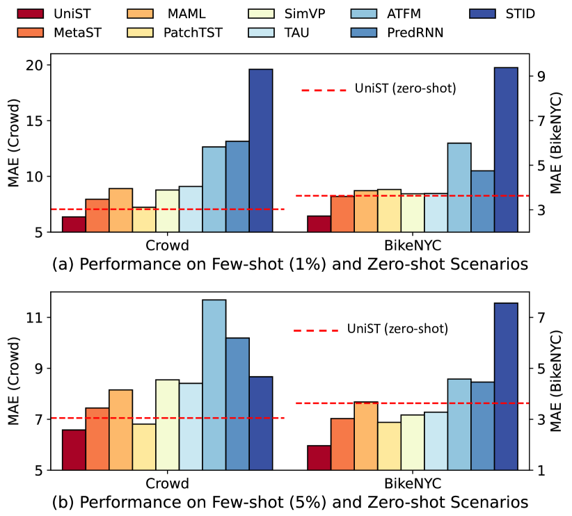
Figure 4. (a) Few-shot performance of UniST and baselines on Crowd and BikeNYC datasets using only 1% of the training data. (b) Few-shot performance of UniST and baselines using only 5% of the training data. The Dashed red lines denote the zero-shot performance of UniST.

5.4. Few-Shot Prediction

Setups.

The hallmark of large foundation models lies in their exceptional generalization ability. The few-shot and zero-shot evaluations are commonly employed to characterize the ultimate tasks for universal time series forecasting (Zhou et al., 2023c; Jin et al., 2023c; Chang et al., 2023). Likewise, the few-shot and zero-shot prediction capability is crucial for a universal spatio-temporal model. In this section, we assess the few-shot learning performance of UniST. Each dataset is partitioned into three segments: training data, validation data, and test data. In few-shot learning scenarios, when confronted with an unseen dataset during the training process, we utilized a restricted amount of training data, specifically, 1%, 5%, 10% of the training data. We choose some baselines with relatively good performance for the few-shot setting evaluation, We also compare with meta-learning baselines, i.e., MAML and MetaST, and pretraining and finetuning-based time series method, i.e., PatchTST.

Results.

Appendix Table 9 to 11 illustrates the overall few-shot results. Due to the space limit, Figure 4 only illustrates the 1% few-shot learning results on two datasets. UniST still outperforms all baselines in few-shot learning scenarios, UniST achieves a larger relative improvement over baselines compared to long-term and short-term predictions. The transferability can be attributed to successful knowledge transfer in our spatio-temporal prompt.

5.5. Zero-Shot Prediction

Setups.

Zero-shot inference serves as the ultimate task for assessing a model’s adaptation ability. In this context, after training on a diverse collection of datasets, we evaluate UniST on an entirely novel dataset—i.e., without any prior training data from it. The test data used in this scenario aligns with that of normal prediction and few-shot prediction.

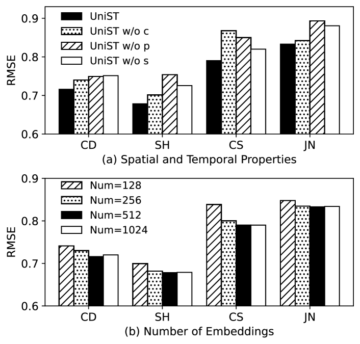
Figure 5. Ablation studies on four traffic speed datasets: Chengdu (CD), Shanghai (SH), Changsha (CS), and Jinan (JN). (a) illustrates the results of removing a prompt guided by one type of spatio-temporal knowledge. (b) presents the results of varying the number of learnable embeddings in the temporal and spatial memory pools.

Results.

Figure 4 also compare the performance of UniST (zero-shot) and baselines (few-shot). As observed, UniST achieves remarkable zero-shot performance, even surpassing many baselines trained with training data that are highlighted by red dashed lines. We attribute these surprising results to the powerful spatio-temporal transfer capability. It suggests that for a completely new scenario, even when the displayed overall patterns are dissimilar to the data encountered during the training process, UniST can extract fine-grained similar patterns from our defined spatial and temporal properties. The few-shot and zero-shot results demonstrate the data-efficient advantage of UniST.

6. Analysis

6.1. Ablation Study

The prompts play an essential role in our UniST model. Here we investigate whether the designed spatial and temporal properties contribute to the final performance. We use ’s’ to denote spatial closeness and hierarchy, ’p’ for temporal periodicity, and ’c’ for temporal closeness. we compare the overall design that incorporates all three properties with three degraded versions that individually remove ’s’, ’p’, or ’c’. Figure 5(a) shows the results on four traffic speed datasets. As we can observe, removing any property results in a performance decrease. The contributions of each spatial and temporal property vary across different datasets, highlighting the necessity of each property for the spatio-temporal design.

Additionally, we explore how the number of embeddings in the memory pools affects the final performance. As seen in Figure 5(b), increasing the number from 128 to 512 improves performance across the four datasets. When further increasing the number to 1024, the performance remains similar to 512, suggesting that 512 is an optimal choice.

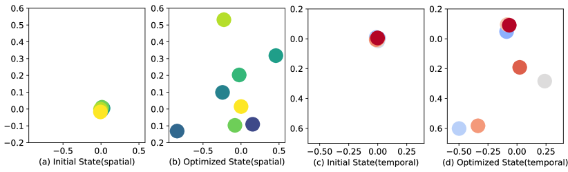
Figure 6. Visualization of embeddings in the spatial and temporal memory pools at the initial and final optimized states. The embeddings exhibit obvious divergence.

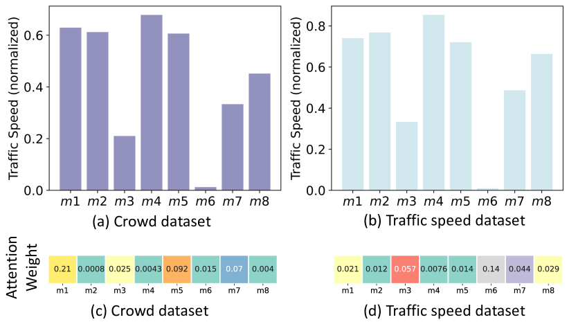
Figure 7. (a) and (b): Comparison of the mean value of inputs in each memory embedding, where the inputs assign the highest attention weight to the memory embedding. Different cities exhibit similar distributions. (c) and (d): Comparison of the attention weight on each memory embedding for two distinct datasets. The two datasets showcase remarkably different distributions.

6.2. Analysis of Prompt Learner

In this section, we conduct in-depth analyses of the prompt learner. To provide a clearer understanding, we leverage t-Distributed Stochastic Neighbor Embedding (t-SNE) to visualize the embeddings of both the spatial and temporal memory pools. Specifically, we plot the initial state and the optimized state in Figure 6. Notably, from the start state to the final optimized state, the embeddings gradually become diverged in different directions. This suggests that, throughout the optimization process, the memory pools progressively store and encapsulate personalized information.

Next, we delve into the memorized patterns of each embedding within the temporal memory pool. Specifically, we first select the inputs based on the attention weights. For each embedding, we aggregate the corresponding input spatio-temporal data with the highest attention weight. Then, we calculate the mean value of the extracted spatio-temporal data. Figure 7(a) and Figure 7(b) illustrates the results for two datasets (Crowd and TrafficSH). As we can see, the memorized patterns revealed in the prompt tool exhibit remarkable consistency across different urban scenarios. This not only affirms that each embedding is meticulously optimized to memorize unique spatio-temporal patterns, but also underscores the robustness of the spatial and temporal memory pools across different scenarios.

Moreover, we examine the extracted spatio-temporal prompts for two distinct domains. Specifically, we calculate the mean attention weight for each embedding in the context of each dataset. Figure 7(c) and Figure 7(d) illustrates the comparison results. As we can observe, the depicted attention weight distributions for the two datasets manifest striking dissimilarities. The observed distinctiveness in attention weight distributions implies a dynamic and responsive nature in the model’s ability to tailor its focus based on the characteristics of the input data. The ability to dynamically adjust the attention weights reinforces UniST’s versatility and universality for diverse datasets.

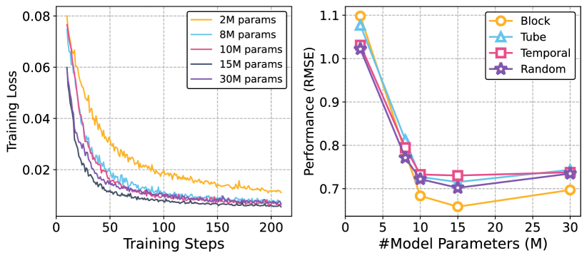
Figure 8. Left: training loss across five models with varying parameter sizes. Right: performance evaluation of masked patch reconstruction by increasing parameter sizes.

6.3. Scalability

We analyze the scalability of our UniST model. Our investigation specifically concentrates on observing changes in training loss and prediction performance as we vary the model parameter size. Figure 8 depicts the training loss and testing RMSE of UniST with varying parameter sizes. For training loss (left figure), we observe two key characteristics: (i) across different parameter sizes, the training loss consistently decreases and gradually converges with increasing training steps; (ii) increazing the parameter size accelerates the convergence of the training loss; (iii) there exist diminishing marginal returns, indicating that the training loss cannot be indefinitely reduced. The right figure illustrates the reconstruction RMSE on the testing set, showing similar trends to the training loss.

7. Conclusion

In this work, we address an important problem: building a universal model UniST for urban spatio-temporal prediction. By leveraging the diversity of spatio-temporal data from multiple sources, and discerning and aligning underlying shared commonalities of spatio-temporal patterns across multiple scenarios, UniST demonstrates a powerful capability to predict across all scenarios, particularly in few-shot and zero-shot settings. The limitation of UniST lies in its reliance on grid-based spatial partitioning. A promising direction for future work entails the integration of various spatio-temporal data formats, such as grid-based, sequence-based, and graph-based data. In essence, the universality of deep learning models holds the promise to bridge the gap between artificial and human intelligence. We believe our study will inspire future research in spatio-temporal modeling towards the universal direction.

Appendix

Appendix A Datasets

Here we provide more details of the used datasets in our study. We collect various spatio-temporal data from multiple cities and domains. Table 3 summarizes the basic information of the used datasets, and Table 4 reports the basic statistics. We have normalized all datasets to the range $[-1,1]$. The reported prediction results are denormalized results. Specifically, values for Crowd and Cellular datasets in Table 1, Table 2, Table 8, Table 9 and Figure 4 should be scaled by a factor of $10^{3}$.

Table 3. The basic information of the used datasets.

Dataset	Domain	City	Temporal Duration	Temporal interval	Spatial partition
TaxiBJ	Taxi GPS	Beijing, China	20130601-20131030	Half an hour	$32\times 32$
			20140301-20140630
			20150301-20150630
			20151101-20160410
Cellular	Cellular usage	Nanjing, China	20201111-20210531	Half an hour	16 * 20
TaxiNYC-1	Taxi OD	New York City, USA	20160101-20160229	Half an hour	16 * 12
TaxiNYC-2	Taxi OD	New York City, USA	20150101-20150301	Half an hour	20 * 10
BikeNYC-1	Bike usage	New York City, USA	20160801-20160929	One hour	16 * 8
BikeNYC-2	Bike usage	New York City, USA	20160701-20160829	Half an hour	10 * 20
TDrive	Taxi trajectory	New York City, USA	20150201-20160602	One hour	$32\times 32$
Crowd	Crowd flow	Nanjing, China	20201111-20210531	Half an hour	16 * 20
TrafficCS	Traffic speed	Changsha, China	20220305-20220405	Five minutes	$28\times 28$
TrafficWH	Traffic speed	Wuhan, China	20220305-20220405	Five minutes	$30\times 28$
TrafficCD	Traffic speed	Chengdu, China	20220305-20220405	Five minutes	$28\times 26$
TrafficJN	Traffic speed	Jinan, China	20220305-20220405	Five minutes	$32\times 18$
TrafficNJ	Traffic speed	Nanjing, China	20220305-20220405	Five minutes	$32\times 24$
TrafficSH	Traffic speed	Shanghai, China	20220127-20220227	Five minutes	$28\times 32$
TrafficSZ	Traffic speed	Shenzhen, China	20220305-20220405	Five minutes	$24\times 18$
TrafficGZ	Traffic speed	Guangzhou, China	20220305-20220405	Five minutes	$32\times 26$
TrafficGY	Traffic speed	Guiyang, China	20220305-20220405	Five minutes	$26\times 28$
TrafficTJ	Traffic speed	Tianjin, China	20220305-20220405	Five minutes	$24\times 30$
TrafficHZ	Traffic speed	Hangzhou, China	20220305-20220405	Five minutes	$28\times 24$
TrafficZZ	Traffic speed	Zhengzhou, China	20220305-20220405	Five minutes	$26\times 26$
TrafficBJ	Traffic speed	Beijing, China	20220305-20220405	Five minutes	$30\times 32$

Table 4. The basic statistics of the used datasets.

Dataset	Min value	Max value	Mean value	Standard deviation
TaxiBJ	0.0	1285	107	133
Cellular	0.0	2992532	75258	149505
TaxiNYC-1	0.0	1517	32	94
TaxiNYC-2	0.0	1283	37	102
BikeNYC-1	0.0	266	9.2	18.1
BikeNYC-2	0.0	299	4.4	14.6
TDrive	0.0	2681	123	229
Crowd	0.0	593118	21656	40825
TrafficCS	0.0	22.25	6.22	4.79
TrafficWH	0.0	22.35	6.22	4.68
TrafficCD	0.0	22.25	7.33	4.36
TrafficJN	0.0	25.04	5.72	4.71
TrafficNJ	0.0	24.82	5.38	4.73
TrafficSH	0.0	21.83	7.92	3.86
TrafficSZ	0.0	22.12	5.11	4.75
TrafficGZ	0.0	25.16	5.26	4.79
TrafficGY	0.0	28.89	5.95	7.03
TrafficTJ	0.0	25.24	6.32	5.05
TrafficHZ	0.0	29.50	3.81	4.38
TrafficZZ	0.0	23.26	6.67	4.32
TrafficBJ	0.0	22.82	6.30	4.22

Appendix B Algorithms

Algorithm 1 Spatio-temporal Pre-training

1:Input: Dataset $D=\{D_{1},D_{2},\ldots,D_{M}\}$, base spatio-temporal prediction model $F$, and loss function $L$.

2:Initialize: Learnable parameters $\theta$ for the model $F$.

3:for $epoch\in\{1,2,\ldots,N_{iter}\}$ do

4:     Randomly sample a dataset $D_{m}$ and a mini-batch $X$ from $D_{m}$.

5:     Randomly choose a masking strategy $M$ from the four strategies.

6:     Mask the input $X$ into $X_{m}$

7:     Compute the reconstructions $\hat{y}\leftarrow F_{\theta}(X_{m})$

8:     Compute the MSE loss $\mathcal{L}\leftarrow L(\hat{y},y)$

9:     Update the model’s parameters $\theta\leftarrow update(\mathcal{L};\theta)$

10:end for

Algorithm 2 Prompt Tuning

1:Input: Dataset $D=\{D_{1},D_{2},\ldots,D_{M}\}$, parameters of pre-trained base model $\theta$, and loss function $L$

2:Initialize: Learnable parameters $\phi$ for the prompt network $G$.

3:Load the pretrained model parameters $\theta$.

4:Fix the parameters of the attention and feed-forward layers of the base model $F_{\theta}$.

5:for $epoch\in\{1,2,\ldots,N_{iter}\}$ do

6:     Randomly sample a dataset $D_{m}$ and a mini-batch $(X,Y)$ from $D_{m}$.

7:     Generate the prompt $P$ for the mini-batch $P\leftarrow G{\phi}(X)$.

8:     Add the prompt to the input space $X_{p}=X+P$.

9:     Compute the predictions $\hat{y}\leftarrow F_{\theta}(X_{p})$

10:     Compute the MSE loss $\mathcal{L}\leftarrow L(\hat{y},Y)$

11:     Update the model’s parameters $\gamma\leftarrow update(\mathcal{L};\gamma),\theta\leftarrow update(\mathcal{L};\theta)$

12:end for

We provide the training algorithm for spatio-temporal pre-trianing on multiple datasets in Algorithm 1. We also present the prompt fine-tuning algorithm in Algorithm 2.

Appendix C Baselines

• HA: History average uses the mean value of historical data for future predictions. Here we use historical data of corresponding periods in the past days.

• ARIMA: Auto-regressive Integrated Moving Average modelis a widely used statistical method for time series forecasting. It is a powerful tool for analyzing and predicting time series data, which are observations collected at regular intervals over time.

• STResNet (Zhang et al., 2017): It is a spatio-temporal model for crowd flow prediction, which utilizes residual neural networks to model the temporal closeness, period, and trend properties.

• ACFM (Liu et al., 2018): Attentive Crowd Flow Machine model is proposed to predict the dynamics of the crowd flows. It learns the dynamics by leveraging an attention mechanism to adaptively aggregate the sequential patterns and the periodic patterns.

• STGSP (Zhao et al., 2022): This model propose that the global information and positional information in the temporal dimension are important for spatio-temproal prediction. To this end, it leverages a semantic flow encoder to model the temporal relative positional signals. Besides, it utilizes an attention mechanism to cpature the multi-scale temporal dependencities.

• MC-STL (Zhang et al., 2023b): It leverages an state-of-the-art training techniques for spatio-temporal predition, the mask-enhanced contrastive learning, which can effectively capture the relationships on the spatio-temporal dimension.

• MAU (Chang et al., 2021): Motion-aware unit is a video predcition model. it broadens the temporal receptive fields of prediction units, which can facilitates to capture inter-frame motion correlations. It consists of an attention module and a fusion module.

• PredRNN (Wang et al., 2017): PredRNN is a recurrent network-based model. In this model, the memory cells are explicitly decoupled, and they calculate in independent transition manners. Besides, different from the memory cell of LSTM, this network leverages zigzap memory flow, which facilitates to learn at distinct levels.

• MIM (Wang et al., 2019): Memory utilize the differential information between adjacent recurrent states, which facilitates to model the non-stationary properties. Stacked multiple MIM blcoks make it possible to model high-order non-stationarity.

• SimVP (Gao et al., 2022a): It is a simple yet very effective video predcition model. It is completely built based on convulutional neural networks and uses MSE loss. It serves as a solid baseline in video prediction tasks.

• TAU (Tan et al., 2023): Temporal Attention Unit is the state-of-the-art video predcition model. It decomposes the temporal attention into two parts: intra-frame attention and inter-frame attention, which are statical and dynamical, respectively. Besides, it introduces a novel regularization, i.e., differential divergence regularization, to consider the impact of inter-frame variations.

• STID (Shao et al., 2022): It is a MLP-based spatio-temporal prediction model, which is simple yet effective. Its superior performance comes from the identification of the indistinguishability of samples in spatio-temporal dimensions. It demonstrates that it is promising to design efficient and effective models in spatio-temporal predictions.

• STNorm (Deng et al., 2021): It proposed two types of normalization modules: spatial normalization and temporal normalization. These two normalizations can separately consider high-frequency components and local components.

• PatchTST (Nie et al., 2022): It first employed patching and self-supervised learning in multivariate time series forecasting. It has two essential designs: (i) segmenting the original time series into patches to capture long-term correlations, (ii) different channels are operated independently, which share the same network.

• iTransformer (Liu et al., 2023b): This is the state-of-the-art multivariate time series model. Different from other Transformer-based methods, it employes the attention and feed-forward operation on an inverted dimension, that is, the multivariate correlation.

• MAML (Finn et al., 2017): Model-Agnostic Meta-Learning is an state-of-the-art meta learning technique. The main idea is to learn a good initialization from various tasks for the target task.

• MetaSTMetaST (Yao et al., 2019): It is a urban transfer learning approach, which utilizes long-period data from multiple cities for transfer learning. by employing a meta-learning approach, it learns a generalized network initialization adaptable to target cities. It also incorporates a pattern-based spatial-temporal memory to capture important patterns.

Appendix D Implementation Details

D.1. Evaluation Metrics

We use commonly used regression metrics, Mean Absolute Error (MAE) and Root Mean Squared Error (RMSE), to measure the prediction performance. Suppose $\bm{Y}=Y_{1},...,Y_{M}$ are ground truth for real spatio-temporal data, $\bm{\hat{Y}}=\hat{Y}_{1},...,\hat{Y}_{N}$ are the predicted values by the model, and $N$ is the number of total testing samples, These two metrics can be formulated as follows:

(12) $$\begin{split}&\mathrm{RMSE}(\bm{Y},\bm{\hat{Y}})=\sqrt{\frac{1}{N}\sum_{i}^{N}\left(Y_{i}-\hat{Y}_{i}\right)^{2}},\\ &\mathrm{MAE}(\bm{Y},\bm{\hat{Y}})=\frac{1}{N}\sum_{i}^{N}\left|Y_{i}-\hat{Y}_{i}\right|,\\ \end{split}$$

D.2. Parameter Settings

Table 5. The parameter details of UniST with different sizes evaluated in ablation studies.

Model	#Encoder Layers	#Decoder Layers	Hidden Dimension (Encoder)	Decoder Hidden Dimension (Decoder)
2M Params	2	2	64	64
8M Params	4	3	128	128
10M Params	6	4	128	128
15M Params	8	8	128	128
30M Params	6	6	256	256

Table 5 shows the parameter details of UniST with different sizes. During the training process, we used the Adam optimizer for gradient-based model optimization. The learning rate of the pre-training is set as 3e-4, and the learning rate of the prompt tuning is set as 5e-5. The pre-training learning rate is selected via grid searching in a set of $\{1e-3,3e-4,1e-4\}$, and the fine-tuning learning rate is selected in a set of $\{1e-4,5e-5,1e-5\}$. Both in pre-training and fine-tuning, we evaluate the model’s performance on the validation set every ten epochs ($\sim$all training instances). We choose the model that performs best on the validation set for evaluations on the testing set.

Appendix E Additional Results

Table 6. Performance comparison of short-term prediction on seven datasets in terms of MAE and RMSE. We use the average prediction errors over all prediction steps.

	TaxiNYC-1		BikeNYC2		TaxiNYC-2		TrafficBJ		TrafficNJ		TrafficWH		TrafficSZ
Model	RMSE	MAE	RMSE	MAE	RMSE	MAE	RMSE	MAE	RMSE	MAE	RMSE	MAE	RMSE	MAE
HA	57.07	18.57	15.68	7.17	52.84	15.74	1.033	0.582	1.593	0.774	1.351	0.645	0.791	0.416
ARIMA	55.39	20.94	25.01	13.63	62.9	29.56	1.32	0.735	1.30	0.709	1.51	0.748	0.821	0.445
STResNet	29.45	17.96	7.18	3.94	22.16	12.06	0.828	0.547	1.03	0.635	0.903	0.568	0.709	0.465
ACFM	23.35	11.54	5.99	3.094	14.48	6.39	0.706	0.44	0.888	0.515	0.784	0.471	0.573	0.35
STID	17.75	7.03	5.70	2.711	17.37	7.35	0.724	0.431	0.847	0.459	0.78	0.436	0.576	0.33
STNorm	21.26	8.14	6.47	3.03	19.02	7.17	0.727	0.428	0.904	0.476	0.81	0.445	0.666	0.369
STGSP	28.13	10.29	14.20	7.38	29.10	10.14	0.736	0.444	0.883	0.491	0.804	0.473	0.86	0.52
MC-STL	18.44	9.51	6.26	3.40	16.78	8.50	0.975	0.709	1.13	0.78	1.1	0.773	0.83	0.615
MAU	28.70	11.23	6.12	2.95	19.38	7.27	1.12	0.797	0.978	0.545	1.37	0.917	0.826	0.523
PredRNN	16.53	5.80	6.47	3.08	19.89	7.23	0.651	0.376	0.852	0.457	0.74	0.421	0.58	0.335
MIM	18.83	6.866	6.36	2.89	18.02	6.56	2.62	2.14	4.65	3.39	3.86	3.15	2.22	1.40
SimVP	16.63	7.51	5.96	2.92	15.10	6.54	0.664	0.408	0.861	0.481	0.779	0.475	0.583	0.359
TAU	16.91	6.85	5.98	2.89	15.35	6.80	0.70	0.44	0.89	0.528	0.747	0.444	0.576	0.353
PatchTST	41.34	13.10	12.33	5.30	37.76	11.13	0.935	0.512	1.379	0.658	1.17	0.561	0.718	0.370
iTransformer	36.73	13.11	9.86	4.50	33.03	11.22	0.876	0.490	1.18	0.60	1.10	0.542	0.718	0.378
PatchTST(one-for-all)	44.43	14.56	13.62	6.03	41.04	12.61	0.964	0.524	1.42	0.675	1.22	0.581	0.739	0.375
UniST (ours)	15.32	5.65	5.50	2.56	12.71	4.82	0.689	0.387	0.845	0.421	0.762	0.396	0.513	0.264

Table 7. Performance comparison of short-term prediction on seven datasets in terms of MAE and RMSE. We use the average prediction errors over all prediction steps.

	TrafficTJ		TrafficGY		TrafficGZ		TrafficZZ		TrafficCS		TrafficCD		TrafficHZ
Model	RMSE	MAE	RMSE	MAE	RMSE	MAE	RMSE	MAE	RMSE	MAE	RMSE	MAE	RMSE	MAE
HA	1.61	0.824	1.79	0.726	0.996	0.52	1.47	0.857	1.31	0.676	1.12	0.668	0.765	0.342
ARIMA	2.02	1.59	1.91	1.16	1.37	0.76	1.78	0.998	1.66	0.923	1.54	0.907	0.803	0.364
STResNet	1.12	0.714	1.32	0.799	0.796	0.515	1.03	0.693	0.986	0.651	0.867	0.576	0.669	0.406
ACFM	0.959	0.574	1.10	0.599	0.701	0.418	0.839	0.526	0.842	0.529	0.757	0.493	0.575	0.316
STID	0.976	0.549	1.04	0.544	0.665	0.362	0.838	0.502	0.855	0.5	0.715	0.44	0.546	0.282
STNorm	0.973	0.533	1.12	0.508	0.693	0.373	0.885	0.538	0.91	0.511	0.786	0.489	0.556	0.260
STGSP	0.989	0.572	1.09	0.649	0.733	0.419	0.831	0.505	0.978	0.587	0.776	0.497	0.616	0.331
MC-STL	1.22	0.856	1.82	1.36	1.04	0.775	1.14	0.81	1.14	0.819	1.00	0.733	0.842	0.606
MAU	0.988	0.549	1.14	0.595	0.74	0.415	1.42	0.934	1.31	0.791	1.25	0.919	0.743	0.377
PredRNN	0.971	0.53	1.16	0.608	0.71	0.42	0.853	0.508	0.909	0.572	0.815	0.513	0.602	0.288
MIM	3.44	2.51	5.68	4.53	3.43	2.80	2.05	1.56	3.57	2.71	2.75	2.26	1.92	1.23
SimVP	1.00	0.597	1.13	0.632	0.667	0.399	0.838	0.526	0.835	0.507	0.775	0.495	0.549	0.301
TAU	1.01	0.606	1.11	0.604	0.65	0.378	0.839	0.527	0.869	0.543	0.768	0.495	0.539	0.289
PatchTST	1.44	0.722	1.58	0.634	0.894	0.448	1.31	0.742	1.18	0.599	1.00	0.577	0.696	0.305
iTransformer	1.26	0.675	1.39	0.621	0.846	0.428	1.19	0.696	1.09	0.572	0.941	0.541	0.66	0.30
PatchTST(one-for-all)	1.49	0.740	1.66	0.684	0.931	0.469	1.35	0.752	1.23	0.620	1.04	0.602	0.726	0.325
UniST (ours)	0.958	0.510	1.03	0.458	0.648	0.325	0.832	0.482	0.791	0.423	0.711	0.415	0.530	0.236

Table 8. Performance comparison of long-term prediction on four datasets in terms of MAE and RMSE. We use the average prediction errors over all prediction steps.

	TaxiBJ		Cellular		BikeNYC-2		TDrive
Model	RMSE	MAE	RMSE	MAE	RMSE	MAE	RMSE	MAE
HA	74.07	43.79	77.29	31.89	15.84	7.97	144.65	72.48
ARIMA	100.76	56.04	83.66	35.96	15.29	7.25	270.05	140.80
STResNet	51.36	36.08	33.87	20.87	12.73	7.16	163.88	112.27
ACFM	35.49	22.46	26.40	13.24	13.00	7.09	88.76	42.19
STID	36.98	23.19	22.98	11.71	12.75	8.37	83.70	37.66
STNorm	33.78	19.89	71.05	32.14	12.16	5.99	100.43	49.50
STGSP	70.31	42.76	67.07	31.16	14.50	7.66	83.70	37.26
MC-STL	38.23	26.86	39.74	27.04	12.72	7.96	100.55	59.18
MAU	85.58	60.61	75.84	32.78	12.42	5.82	137.17	76.17
PredRNN	43.89	27.42	46.68	24.96	9.72	4.37	175.32	104.79
MIM	38.10	25.82	79.20	39.27	10.02	4.60	107.06	43.67
SimVP	33.53	19.28	23.84	12.90	10.89	5.51	91.13	39.46
TAU	34.88	19.94	23.00	12.72	11.53	6.11	91.54	41.96
PatchTST	30.64	17.49	23.39	12.42	11.13	5.07	92.03	38.89
PatchTST(one-for-all)	31.58	18.67	27.94	10.89	10.71	4.74	111.56	50.57
iTransformer	32.89	18.60	29.329	11.963	11.54	5.19	93.87	40.16
UniST (ours)	30.46	17.95	20.64	10.43	11.91	5.06	90.60	37.01

Table 9. Performance comparison in few-shot and zero-shot (only UniST) learning settings on the Crowd dataset in terms of MAE and RMSE. 1% , 5%, and 10% denote that only the percentage of training data is utilized. We use the average prediction errors over all prediction steps.

	10%		5%		1%
Model	RMSE	MAE	RMSE	MAE	RMSE	MAE
ATFM	19.842	11.446	19.923	11.687	21.166	12.643
STNorm	14.668	7.050	14.884	7.723	35.959	29.585
STID	14.676	7.280	14.975	8.671	25.905	19.610
PredRNN	19.604	9.668	20.186	10.190	24.901	13.142
SimVP	14.093	7.101	14.167	8.550	14.252	8.776
TAU	14.229	7.140	14.456	8.411	14.919	9.096
MAML	14.089	7.180	14.795	8.154	14.334	8.608
MetaST	13.801	6.847	14.220	7.442	14.242	7.949
PatchTST	14.060	6.787	14.142	6.811	14.491	7.227
UniST (few-shot)	13.411	6.365	13.859	6.542	13.952	6.581
UniST (zero-shot)	14.665	7.051	14.665	7.051	14.665	7.051

Table 10. Performance comparison in few-shot and zero-shot (only UniST) learning settings on the BikeNYC dataset in terms of MAE and RMSE. 1% , 5%, and 10% denote that only the percentage of training data is utilized. We use the average prediction errors over all prediction steps.

	10%		5%		1%
Model	RMSE	MAE	RMSE	MAE	RMSE	MAE
ATFM	8.026	3.511	10.438	4.582	11.876	5.990
STNorm	7.42	2.70	10.21	4.17	12.94	5.20
STID	6.97	3.49	12.46	7.56	15.08	9.38
PredRNN	11.05	4.00	11.29	4.46	12.58	4.75
SimVP	6.570	2.691	8.525	3.174	8.661	3.721
TAU	7.06	3.07	8.74	3.28	8.50	3.72
MAML	6.49	2.31	8.89	3.68	8.98	3.91
MetaST	6.21	2.18	8.22	3.03	8.58	3.60
PatchTST	9.14	2.68	10.09	2.88	9.74	3.86
UniST	5.318	1.668	6.113	1.964	7.811	2.72
UniST (zero-shot)	9.06	3.63	9.06	3.63	9.06	3.63

Table 11. Performance comparison in few-shot and zero-shot (only UniST) learning settings on the TaxiBJ dataset in terms of MAE and RMSE. 1% , 5%, and 10% denote that only the percentage of training data is utilized. We use the average prediction errors over all prediction steps.

	10%		5%		1%
Model	RMSE	MAE	RMSE	MAE	RMSE	MAE
ATFM	50.631	33.035	55.770	39.205	64.590	44.928
STNorm	39.35	22.48	42.67	26.78	44.76	28.24
STID	34.53	20.54	37.39	24.35	47.94	31.94
PredRNN	84.28	58.52	97.74	73.40	92.21	66.76
SimVP	35.114	20.87	37.42	23.131	40.465	24.95
TAU	37.70	22.69	39.77	25.73	41.98	26.48
MAML	36.24	20.91	36.12	23.47	40.11	24.79
MetaST	35.42	18.65	35.21	21.74	39.08	23.88
PatchTST	44.03	22.69	44.24	22.62	46.43	24.77
UniST	27.59	15.18	31.19	17.58	35.09	20.62
UniST (zero-shot)	51.4	33.1	51.4	33.1	51.4	33.1

References

- (1)
- Tra (2023) 2023. TransGPT. https://github.com/DUOMO/TransGPT
- Bai et al. (2019b) Lei Bai, Lina Yao, Salil Kanhere, Xianzhi Wang, Quan Sheng, et al. 2019b. Stg2seq: Spatial-temporal graph to sequence model for multi-step passenger demand forecasting. arXiv preprint arXiv:1905.10069 (2019).
- Bai et al. (2019a) Lei Bai, Lina Yao, Salil S Kanhere, Xianzhi Wang, Wei Liu, and Zheng Yang. 2019a. Spatio-temporal graph convolutional and recurrent networks for citywide passenger demand prediction. In Proceedings of the 28th ACM International Conference on Information and Knowledge Management. 2293–2296.
- Bai et al. (2019c) Lei Bai, Lina Yao, Salil S Kanhere, Zheng Yang, Jing Chu, and Xianzhi Wang. 2019c. Passenger demand forecasting with multi-task convolutional recurrent neural networks. In Advances in Knowledge Discovery and Data Mining: 23rd Pacific-Asia Conference, PAKDD 2019, Macau, China, April 14-17, 2019, Proceedings, Part II 23. Springer, 29–42.
- Bai et al. (2020) Lei Bai, Lina Yao, Can Li, Xianzhi Wang, and Can Wang. 2020. Adaptive graph convolutional recurrent network for traffic forecasting. Advances in neural information processing systems 33 (2020), 17804–17815.
- Bai et al. (2023) Yutong Bai, Xinyang Geng, Karttikeya Mangalam, Amir Bar, Alan Yuille, Trevor Darrell, Jitendra Malik, and Alexei A Efros. 2023. Sequential modeling enables scalable learning for large vision models. arXiv preprint arXiv:2312.00785 (2023).
- Brown et al. (2020) Tom Brown, Benjamin Mann, Nick Ryder, Melanie Subbiah, Jared D Kaplan, Prafulla Dhariwal, Arvind Neelakantan, Pranav Shyam, Girish Sastry, Amanda Askell, et al. 2020. Language models are few-shot learners. Advances in neural information processing systems 33 (2020), 1877–1901.
- Cao et al. (2023) Defu Cao, Furong Jia, Sercan O Arik, Tomas Pfister, Yixiang Zheng, Wen Ye, and Yan Liu. 2023. Tempo: Prompt-based generative pre-trained transformer for time series forecasting. arXiv preprint arXiv:2310.04948 (2023).
- Chang et al. (2023) Ching Chang, Wen-Chih Peng, and Tien-Fu Chen. 2023. Llm4ts: Two-stage fine-tuning for time-series forecasting with pre-trained llms. arXiv preprint arXiv:2308.08469 (2023).
- Chang et al. (2021) Zheng Chang, Xinfeng Zhang, Shanshe Wang, Siwei Ma, Yan Ye, Xiang Xinguang, and Wen Gao. 2021. Mau: A motion-aware unit for video prediction and beyond. Advances in Neural Information Processing Systems 34 (2021), 26950–26962.
- Chen et al. (2022) Changlu Chen, Yanbin Liu, Ling Chen, and Chengqi Zhang. 2022. Bidirectional spatial-temporal adaptive transformer for Urban traffic flow forecasting. IEEE Transactions on Neural Networks and Learning Systems (2022).
- Chen et al. (2023) Jie Chen, Tong Liu, and Ruiyuan Li. 2023. Region Profile Enhanced Urban Spatio-Temporal Prediction via Adaptive Meta-Learning. In Proceedings of the 32nd ACM International Conference on Information and Knowledge Management. 224–233.
- Chen et al. (2021) Weihuang Chen, Fangfang Wang, and Hongbin Sun. 2021. S2tnet: Spatio-temporal transformer networks for trajectory prediction in autonomous driving. In Asian Conference on Machine Learning. PMLR, 454–469.
- Cheng et al. (2023) Jinguo Cheng, Ke Li, Yuxuan Liang, Lijun Sun, Junchi Yan, and Yuankai Wu. 2023. Rethinking Urban Mobility Prediction: A Super-Multivariate Time Series Forecasting Approach. arXiv preprint arXiv:2312.01699 (2023).
- Da et al. (2023) Longchao Da, Kuanru Liou, Tiejin Chen, Xuesong Zhou, Xiangyong Luo, Yezhou Yang, and Hua Wei. 2023. Open-TI: Open Traffic Intelligence with Augmented Language Model. arXiv preprint arXiv:2401.00211 (2023).
- Deng et al. (2021) Jinliang Deng, Xiusi Chen, Renhe Jiang, Xuan Song, and Ivor W Tsang. 2021. St-norm: Spatial and temporal normalization for multi-variate time series forecasting. In Proceedings of the 27th ACM SIGKDD conference on knowledge discovery & data mining. 269–278.
- Devlin et al. (2018) Jacob Devlin, Ming-Wei Chang, Kenton Lee, and Kristina Toutanova. 2018. Bert: Pre-training of deep bidirectional transformers for language understanding. arXiv preprint arXiv:1810.04805 (2018).
- Fang et al. (2022) Ziquan Fang, Dongen Wu, Lu Pan, et al. 2022. When transfer learning meets cross-city urban flow prediction: spatio-temporal adaptation matters. IJCAI’22 (2022), 2030–2036.
- Finn et al. (2017) Chelsea Finn, Pieter Abbeel, and Sergey Levine. 2017. Model-agnostic meta-learning for fast adaptation of deep networks. In International conference on machine learning. PMLR, 1126–1135.
- Gao et al. (2022b) Nan Gao, Hao Xue, Wei Shao, Sichen Zhao, Kyle Kai Qin, Arian Prabowo, Mohammad Saiedur Rahaman, and Flora D Salim. 2022b. Generative adversarial networks for spatio-temporal data: A survey. ACM Transactions on Intelligent Systems and Technology (TIST) 13, 2 (2022), 1–25.
- Gao et al. (2022a) Zhangyang Gao, Cheng Tan, Lirong Wu, and Stan Z Li. 2022a. Simvp: Simpler yet better video prediction. In Proceedings of the IEEE/CVF Conference on Computer Vision and Pattern Recognition. 3170–3180.
- Garza and Mergenthaler-Canseco (2023) Azul Garza and Max Mergenthaler-Canseco. 2023. TimeGPT-1. arXiv preprint arXiv:2310.03589 (2023).
- Geng et al. (2019) Xu Geng, Yaguang Li, Leye Wang, Lingyu Zhang, Qiang Yang, Jieping Ye, and Yan Liu. 2019. Spatiotemporal multi-graph convolution network for ride-hailing demand forecasting. In Proceedings of the AAAI conference on artificial intelligence, Vol. 33. 3656–3663.
- He et al. (2022) Kaiming He, Xinlei Chen, Saining Xie, Yanghao Li, Piotr Dollár, and Ross Girshick. 2022. Masked autoencoders are scalable vision learners. In Proceedings of the IEEE/CVF conference on computer vision and pattern recognition. 16000–16009.
- Ji et al. (2023) Jiahao Ji, Jingyuan Wang, Chao Huang, Junjie Wu, Boren Xu, Zhenhe Wu, Junbo Zhang, and Yu Zheng. 2023. Spatio-temporal self-supervised learning for traffic flow prediction. In Proceedings of the AAAI conference on artificial intelligence, Vol. 37. 4356–4364.
- Jia et al. (2022) Menglin Jia, Luming Tang, Bor-Chun Chen, Claire Cardie, Serge Belongie, Bharath Hariharan, and Ser-Nam Lim. 2022. Visual prompt tuning. In European Conference on Computer Vision. Springer, 709–727.
- Jiang et al. (2023a) Jiawei Jiang, Chengkai Han, Wayne Xin Zhao, and Jingyuan Wang. 2023a. PDFormer: Propagation Delay-aware Dynamic Long-range Transformer for Traffic Flow Prediction. arXiv preprint arXiv:2301.07945 (2023).
- Jiang et al. (2023b) Renhe Jiang, Zhaonan Wang, Jiawei Yong, Puneet Jeph, Quanjun Chen, Yasumasa Kobayashi, Xuan Song, Shintaro Fukushima, and Toyotaro Suzumura. 2023b. Spatio-temporal meta-graph learning for traffic forecasting. In Proceedings of the AAAI conference on artificial intelligence, Vol. 37. 8078–8086.
- Jin et al. (2023b) Guangyin Jin, Yuxuan Liang, Yuchen Fang, Zezhi Shao, Jincai Huang, Junbo Zhang, and Yu Zheng. 2023b. Spatio-temporal graph neural networks for predictive learning in urban computing: A survey. IEEE Transactions on Knowledge and Data Engineering (2023).
- Jin et al. (2023c) Ming Jin, Shiyu Wang, Lintao Ma, Zhixuan Chu, James Y Zhang, Xiaoming Shi, Pin-Yu Chen, Yuxuan Liang, Yuan-Fang Li, Shirui Pan, et al. 2023c. Time-llm: Time series forecasting by reprogramming large language models. arXiv preprint arXiv:2310.01728 (2023).
- Jin et al. (2023d) Ming Jin, Qingsong Wen, Yuxuan Liang, Chaoli Zhang, Siqiao Xue, Xue Wang, James Zhang, Yi Wang, Haifeng Chen, Xiaoli Li, et al. 2023d. Large models for time series and spatio-temporal data: A survey and outlook. arXiv preprint arXiv:2310.10196 (2023).
- Jin et al. (2022) Yilun Jin, Kai Chen, and Qiang Yang. 2022. Selective cross-city transfer learning for traffic prediction via source city region re-weighting. In Proceedings of the 28th ACM SIGKDD Conference on Knowledge Discovery and Data Mining. 731–741.
- Jin et al. (2023a) Yilun Jin, Kai Chen, and Qiang Yang. 2023a. Transferable graph structure learning for graph-based traffic forecasting across cities. In Proceedings of the 29th ACM SIGKDD Conference on Knowledge Discovery and Data Mining. 1032–1043.
- Kirillov et al. (2023) Alexander Kirillov, Eric Mintun, Nikhila Ravi, Hanzi Mao, Chloe Rolland, Laura Gustafson, Tete Xiao, Spencer Whitehead, Alexander C Berg, Wan-Yen Lo, et al. 2023. Segment anything. arXiv preprint arXiv:2304.02643 (2023).
- Kojima et al. (2022) Takeshi Kojima, Shixiang Shane Gu, Machel Reid, Yutaka Matsuo, and Yusuke Iwasawa. 2022. Large language models are zero-shot reasoners. Advances in neural information processing systems 35 (2022), 22199–22213.
- Lai et al. (2023) Siqi Lai, Zhao Xu, Weijia Zhang, Hao Liu, and Hui Xiong. 2023. Large Language Models as Traffic Signal Control Agents: Capacity and Opportunity. arXiv preprint arXiv:2312.16044 (2023).
- Li et al. (2018) Yaguang Li, Rose Yu, Cyrus Shahabi, and Yan Liu. 2018. Diffusion Convolutional Recurrent Neural Network: Data-Driven Traffic Forecasting. In International Conference on Learning Representations.
- Liang et al. (2018) Yuxuan Liang, Songyu Ke, Junbo Zhang, Xiuwen Yi, and Yu Zheng. 2018. Geoman: Multi-level attention networks for geo-sensory time series prediction.. In IJCAI, Vol. 2018. 3428–3434.
- Liang et al. (2019) Yuxuan Liang, Kun Ouyang, Lin Jing, Sijie Ruan, Ye Liu, Junbo Zhang, David S Rosenblum, and Yu Zheng. 2019. Urbanfm: Inferring fine-grained urban flows. In Proceedings of the 25th ACM SIGKDD international conference on knowledge discovery & data mining. 3132–3142.
- Liang et al. (2021a) Yuxuan Liang, Kun Ouyang, Junkai Sun, Yiwei Wang, Junbo Zhang, Yu Zheng, David Rosenblum, and Roger Zimmermann. 2021a. Fine-grained urban flow prediction. In Proceedings of the Web Conference 2021. 1833–1845.
- Liang et al. (2021b) Yuxuan Liang, Kun Ouyang, Yiwei Wang, Ye Liu, Junbo Zhang, Yu Zheng, and David S Rosenblum. 2021b. Revisiting convolutional neural networks for citywide crowd flow analytics. In Machine Learning and Knowledge Discovery in Databases: European Conference, ECML PKDD 2020, Ghent, Belgium, September 14–18, 2020, Proceedings, Part I. Springer, 578–594.
- Lin et al. (2020) Zhihui Lin, Maomao Li, Zhuobin Zheng, Yangyang Cheng, and Chun Yuan. 2020. Self-attention convlstm for spatiotemporal prediction. In Proceedings of the AAAI conference on artificial intelligence, Vol. 34. 11531–11538.
- Liu et al. (2018) Lingbo Liu, Ruimao Zhang, Jiefeng Peng, Guanbin Li, Bowen Du, and Liang Lin. 2018. Attentive crowd flow machines. In Proceedings of the 26th ACM international conference on Multimedia. 1553–1561.
- Liu et al. (2023d) Pengfei Liu, Weizhe Yuan, Jinlan Fu, Zhengbao Jiang, Hiroaki Hayashi, and Graham Neubig. 2023d. Pre-train, prompt, and predict: A systematic survey of prompting methods in natural language processing. Comput. Surveys 55, 9 (2023), 1–35.
- Liu et al. (2023a) Xu Liu, Junfeng Hu, Yuan Li, Shizhe Diao, Yuxuan Liang, Bryan Hooi, and Roger Zimmermann. 2023a. UniTime: A Language-Empowered Unified Model for Cross-Domain Time Series Forecasting. arXiv preprint arXiv:2310.09751 (2023).
- Liu et al. (2022) Xu Liu, Yuxuan Liang, Chao Huang, Yu Zheng, Bryan Hooi, and Roger Zimmermann. 2022. When do contrastive learning signals help spatio-temporal graph forecasting?. In Proceedings of the 30th International Conference on Advances in Geographic Information Systems. 1–12.
- Liu et al. (2023b) Yong Liu, Tengge Hu, Haoran Zhang, Haixu Wu, Shiyu Wang, Lintao Ma, and Mingsheng Long. 2023b. itransformer: Inverted transformers are effective for time series forecasting. arXiv preprint arXiv:2310.06625 (2023).
- Liu et al. (2023c) Yong Liu, Chenyu Li, Jianmin Wang, and Mingsheng Long. 2023c. Koopa: Learning Non-stationary Time Series Dynamics with Koopman Predictors. arXiv preprint arXiv:2305.18803 (2023).
- Liu et al. (2023e) Zhanyu Liu, Guanjie Zheng, and Yanwei Yu. 2023e. Cross-city Few-Shot Traffic Forecasting via Traffic Pattern Bank. In Proceedings of the 32nd ACM International Conference on Information and Knowledge Management. 1451–1460.
- Lu et al. (2022) Bin Lu, Xiaoying Gan, Weinan Zhang, Huaxiu Yao, Luoyi Fu, and Xinbing Wang. 2022. Spatio-Temporal Graph Few-Shot Learning with Cross-City Knowledge Transfer. In Proceedings of the 28th ACM SIGKDD Conference on Knowledge Discovery and Data Mining. 1162–1172.
- Nie et al. (2022) Yuqi Nie, Nam H Nguyen, Phanwadee Sinthong, and Jayant Kalagnanam. 2022. A time series is worth 64 words: Long-term forecasting with transformers. arXiv preprint arXiv:2211.14730 (2022).
- Ouyang et al. (2023) Xiaocao Ouyang, Yan Yang, Wei Zhou, Yiling Zhang, Hao Wang, and Wei Huang. 2023. CityTrans: Domain-Adversarial Training with Knowledge Transfer for Spatio-Temporal Prediction across Cities. IEEE Transactions on Knowledge and Data Engineering (2023).
- Pan et al. (2019) Zheyi Pan, Yuxuan Liang, Weifeng Wang, Yong Yu, Yu Zheng, and Junbo Zhang. 2019. Urban traffic prediction from spatio-temporal data using deep meta learning. In Proceedings of the 25th ACM SIGKDD international conference on knowledge discovery & data mining. 1720–1730.
- Pan et al. (2020) Zheyi Pan, Wentao Zhang, Yuxuan Liang, Weinan Zhang, Yong Yu, Junbo Zhang, and Yu Zheng. 2020. Spatio-temporal meta learning for urban traffic prediction. IEEE Transactions on Knowledge and Data Engineering 34, 3 (2020), 1462–1476.
- Qiao et al. (2022) Shuofei Qiao, Yixin Ou, Ningyu Zhang, Xiang Chen, Yunzhi Yao, Shumin Deng, Chuanqi Tan, Fei Huang, and Huajun Chen. 2022. Reasoning with language model prompting: A survey. arXiv preprint arXiv:2212.09597 (2022).
- Rombach et al. (2022) Robin Rombach, Andreas Blattmann, Dominik Lorenz, Patrick Esser, and Björn Ommer. 2022. High-resolution image synthesis with latent diffusion models. In Proceedings of the IEEE/CVF conference on computer vision and pattern recognition. 10684–10695.
- Shao et al. (2022) Zezhi Shao, Zhao Zhang, Fei Wang, Wei Wei, and Yongjun Xu. 2022. Spatial-temporal identity: A simple yet effective baseline for multivariate time series forecasting. In Proceedings of the 31st ACM International Conference on Information & Knowledge Management. 4454–4458.
- Shen et al. (2024) Sheng Shen, Shijia Yang, Tianjun Zhang, Bohan Zhai, Joseph E Gonzalez, Kurt Keutzer, and Trevor Darrell. 2024. Multitask vision-language prompt tuning. In Proceedings of the IEEE/CVF Winter Conference on Applications of Computer Vision. 5656–5667.
- Sukhbaatar et al. (2015) Sainbayar Sukhbaatar, Jason Weston, Rob Fergus, et al. 2015. End-to-end memory networks. Advances in neural information processing systems 28 (2015).
- Tan et al. (2023) Cheng Tan, Zhangyang Gao, Lirong Wu, Yongjie Xu, Jun Xia, Siyuan Li, and Stan Z Li. 2023. Temporal attention unit: Towards efficient spatiotemporal predictive learning. In Proceedings of the IEEE/CVF Conference on Computer Vision and Pattern Recognition. 18770–18782.
- Tang et al. (2023) Jiabin Tang, Lianghao Xia, Jie Hu, and Chao Huang. 2023. Spatio-Temporal Meta Contrastive Learning. In Proceedings of the 32nd ACM International Conference on Information and Knowledge Management. 2412–2421.
- Tang et al. (2022) Yihong Tang, Ao Qu, Andy HF Chow, William HK Lam, SC Wong, and Wei Ma. 2022. Domain adversarial spatial-temporal network: a transferable framework for short-term traffic forecasting across cities. In Proceedings of the 31st ACM International Conference on Information & Knowledge Management. 1905–1915.
- Touvron et al. (2023) Hugo Touvron, Louis Martin, Kevin Stone, Peter Albert, Amjad Almahairi, Yasmine Babaei, Nikolay Bashlykov, Soumya Batra, Prajjwal Bhargava, Shruti Bhosale, et al. 2023. Llama 2: Open foundation and fine-tuned chat models. arXiv preprint arXiv:2307.09288 (2023).
- Wang et al. (2018b) Leye Wang, Xu Geng, Xiaojuan Ma, Feng Liu, and Qiang Yang. 2018b. Cross-city transfer learning for deep spatio-temporal prediction. arXiv preprint arXiv:1802.00386 (2018).
- Wang et al. (2020) Senzhang Wang, Jiannong Cao, and S Yu Philip. 2020. Deep learning for spatio-temporal data mining: A survey. IEEE transactions on knowledge and data engineering 34, 8 (2020), 3681–3700.
- Wang et al. (2018a) Yunbo Wang, Zhifeng Gao, Mingsheng Long, Jianmin Wang, and S Yu Philip. 2018a. Predrnn++: Towards a resolution of the deep-in-time dilemma in spatiotemporal predictive learning. In International Conference on Machine Learning. PMLR, 5123–5132.
- Wang et al. (2017) Yunbo Wang, Mingsheng Long, Jianmin Wang, Zhifeng Gao, and Philip S Yu. 2017. Predrnn: Recurrent neural networks for predictive learning using spatiotemporal lstms. Advances in neural information processing systems 30 (2017).
- Wang et al. (2019) Yunbo Wang, Jianjin Zhang, Hongyu Zhu, Mingsheng Long, Jianmin Wang, and Philip S Yu. 2019. Memory in memory: A predictive neural network for learning higher-order non-stationarity from spatiotemporal dynamics. In Proceedings of the IEEE/CVF conference on computer vision and pattern recognition. 9154–9162.
- Wang et al. (2023) Zhenyu Wang, Yali Li, Xi Chen, Ser-Nam Lim, Antonio Torralba, Hengshuang Zhao, and Shengjin Wang. 2023. Detecting everything in the open world: Towards universal object detection. In Proceedings of the IEEE/CVF Conference on Computer Vision and Pattern Recognition. 11433–11443.
- Wang et al. (2022) Zifeng Wang, Zizhao Zhang, Chen-Yu Lee, Han Zhang, Ruoxi Sun, Xiaoqi Ren, Guolong Su, Vincent Perot, Jennifer Dy, and Tomas Pfister. 2022. Learning to prompt for continual learning. In Proceedings of the IEEE/CVF Conference on Computer Vision and Pattern Recognition. 139–149.
- Wen et al. (2023) Haomin Wen, Youfang Lin, Yutong Xia, Huaiyu Wan, Qingsong Wen, Roger Zimmermann, and Yuxuan Liang. 2023. Diffstg: Probabilistic spatio-temporal graph forecasting with denoising diffusion models. In Proceedings of the 31st ACM International Conference on Advances in Geographic Information Systems. 1–12.
- Wu et al. (2022) Haixu Wu, Tengge Hu, Yong Liu, Hang Zhou, Jianmin Wang, and Mingsheng Long. 2022. Timesnet: Temporal 2d-variation modeling for general time series analysis. arXiv preprint arXiv:2210.02186 (2022).
- Xia et al. (2023) Yutong Xia, Yuxuan Liang, Haomin Wen, Xu Liu, Kun Wang, Zhengyang Zhou, and Roger Zimmermann. 2023. Deciphering spatio-temporal graph forecasting: A causal lens and treatment. arXiv preprint arXiv:2309.13378 (2023).
- Xu et al. (2023) Fengli Xu, Jun Zhang, Chen Gao, Jie Feng, and Yong Li. 2023. Urban Generative Intelligence (UGI): A Foundational Platform for Agents in Embodied City Environment. arXiv preprint arXiv:2312.11813 (2023).
- Yan et al. (2023) Yibo Yan, Haomin Wen, Siru Zhong, Wei Chen, Haodong Chen, Qingsong Wen, Roger Zimmermann, and Yuxuan Liang. 2023. When Urban Region Profiling Meets Large Language Models. arXiv preprint arXiv:2310.18340 (2023).
- Yao et al. (2019) Huaxiu Yao, Yiding Liu, Ying Wei, Xianfeng Tang, and Zhenhui Li. 2019. Learning from multiple cities: A meta-learning approach for spatial-temporal prediction. In The world wide web conference. 2181–2191.
- Yu et al. (2020) Cunjun Yu, Xiao Ma, Jiawei Ren, Haiyu Zhao, and Shuai Yi. 2020. Spatio-temporal graph transformer networks for pedestrian trajectory prediction. In Computer Vision–ECCV 2020: 16th European Conference, Glasgow, UK, August 23–28, 2020, Proceedings, Part XII 16. Springer, 507–523.
- Yuan et al. (2023) Yuan Yuan, Jingtao Ding, Chenyang Shao, Depeng Jin, and Yong Li. 2023. Spatio-temporal Diffusion Point Processes. arXiv preprint arXiv:2305.12403 (2023).
- Zhang et al. (2017) Junbo Zhang, Yu Zheng, and Dekang Qi. 2017. Deep spatio-temporal residual networks for citywide crowd flows prediction. In Proceedings of the AAAI conference on artificial intelligence, Vol. 31.
- Zhang et al. (2023a) Siyao Zhang, Daocheng Fu, Zhao Zhang, Bin Yu, and Pinlong Cai. 2023a. Trafficgpt: Viewing, processing and interacting with traffic foundation models. arXiv preprint arXiv:2309.06719 (2023).
- Zhang et al. (2023b) Xu Zhang, Yongshun Gong, Xinxin Zhang, Xiaoming Wu, Chengqi Zhang, and Xiangjun Dong. 2023b. Mask-and Contrast-Enhanced Spatio-Temporal Learning for Urban Flow Prediction. In Proceedings of the 32nd ACM International Conference on Information and Knowledge Management. 3298–3307.
- Zhang et al. (2023c) Zijian Zhang, Ze Huang, Zhiwei Hu, Xiangyu Zhao, Wanyu Wang, Zitao Liu, Junbo Zhang, S Joe Qin, and Hongwei Zhao. 2023c. MLPST: MLP is All You Need for Spatio-Temporal Prediction. In Proceedings of the 32nd ACM International Conference on Information and Knowledge Management. 3381–3390.
- Zhao et al. (2022) Liang Zhao, Min Gao, and Zongwei Wang. 2022. St-gsp: Spatial-temporal global semantic representation learning for urban flow prediction. In Proceedings of the Fifteenth ACM International Conference on Web Search and Data Mining. 1443–1451.
- Zhao et al. (2019) Ling Zhao, Yujiao Song, Chao Zhang, Yu Liu, Pu Wang, Tao Lin, Min Deng, and Haifeng Li. 2019. T-gcn: A temporal graph convolutional network for traffic prediction. IEEE transactions on intelligent transportation systems 21, 9 (2019), 3848–3858.
- Zheng et al. (2014) Yu Zheng, Licia Capra, Ouri Wolfson, and Hai Yang. 2014. Urban computing: concepts, methodologies, and applications. ACM Transactions on Intelligent Systems and Technology (TIST) 5, 3 (2014), 1–55.
- Zhou et al. (2023c) Tian Zhou, Peisong Niu, Xue Wang, Liang Sun, and Rong Jin. 2023c. One Fits All: Power General Time Series Analysis by Pretrained LM. arXiv preprint arXiv:2302.11939 (2023).
- Zhou et al. (2023a) Zhilun Zhou, Jingtao Ding, Yu Liu, Depeng Jin, and Yong Li. 2023a. Towards Generative Modeling of Urban Flow through Knowledge-enhanced Denoising Diffusion. In Proceedings of the 31st ACM International Conference on Advances in Geographic Information Systems. 1–12.
- Zhou et al. (2023b) Zhengyang Zhou, Qihe Huang, Kuo Yang, Kun Wang, Xu Wang, Yudong Zhang, Yuxuan Liang, and Yang Wang. 2023b. Maintaining the Status Quo: Capturing Invariant Relations for OOD Spatiotemporal Learning. (2023).
- Zhou et al. (2023d) Zhengyang Zhou, Kuo Yang, Yuxuan Liang, Binwu Wang, Hongyang Chen, and Yang Wang. 2023d. Predicting collective human mobility via countering spatiotemporal heterogeneity. IEEE Transactions on Mobile Computing (2023).