A novel framework for adaptive stress testing of autonomous vehicles in highways

Abstract

Guaranteeing the safe operations of autonomous vehicles (AVs) is crucial for their widespread adoption and public acceptance. It is thus of a great significance to not only assess the AV against the standard safety tests, but also discover potential corner cases of the AV under test that could lead to unsafe behaviour or scenario. In this paper, we propose a novel framework to systematically explore corner cases that can result in safety concerns in a highway traffic scenario. The framework is based on an adaptive stress testing (AST) approach, an emerging validation method that leverages a Markov decision process to formulate the scenarios and deep reinforcement learning (DRL) to discover the desirable patterns representing corner cases. To this end, we develop a new reward function for DRL to guide the AST in identifying crash scenarios based on the collision probability estimate between the AV under test (i.e., the ego vehicle) and the trajectory of other vehicles on the highway. The proposed framework is further integrated with a new driving model enabling us to create more realistic traffic scenarios capturing both the longitudinal and lateral movements of vehicles on the highway. In our experiment, we calibrate our model using real-world crash statistics involving automated vehicles in California, and then we analyze the characteristics of the AV and the framework. Quantitative and qualitative analyses of our experimental results demonstrate that our framework outperforms other existing AST schemes. The study can help discover crash scenarios of AV that are unknown or absent in human driving, thereby enhancing the safety and trustworthiness of AV technology.

[label1]organization=Department of Civil Engineering, Monash University,addressline=14 Alliance Lane, city=Clayton, postcode=3168, state=Victoria, country=Australia

[label2]organization=Department of Computing Technologies,addressline=1 John Street, city=Hawthorn, postcode=3122, state=Victoria, country=Australia

1 Introduction

Ensuring the safe operations of autonomous vehicles (AVs) is essential for their broad acceptance and public trust. Verification and validation are crucial to the safety of AV systems at all stages of their development from simulations to on-road testing. Conventional testing methods often require the existence of known scenarios which will later be used for verifying the AVs at the system level. Identifying such scenarios in different operational design domains (ODD) (SAE, 2018) is of a great challenge due to many possible variants that can occur in reality (Beringhoff et al., 2022).

An emerging approach, namely, adaptive stress testing (AST), can address this challenge using the bottom up perspective (Corso et al., 2019; Lytskjold and Mengshoel, 2023; Hjelmeland et al., 2022). The goal of this approach is to identify potential failure scenarios and their likelihoods of occurrences. In particular, it is designed to discover the most probable system failure events, which are traditionally formulated as a Markov Decision Process (MDP) (Ritchie et al., 2015; Mark et al., 2018). In this process, Reinforcement learning (RL) is often employed in conjunction with domain knowledge to efficiently explore the vast state space and identify failure events. To this end, the search process is guided by a reward function that encourages failures such as collisions and near-misses with a high transition probability. In the literature, it has recently been used to explore the failure patterns of the intelligent driving model (IDM) under test (Zhang et al., 2023). Prior to the application in self-driving in traffic, AST has shown great successes in numerous other relating applications, including the evaluation of aircraft collision avoidance (Ritchie et al., 2015), maritime collision avoidance (Hjelmeland et al., 2022; Lytskjold and Mengshoel, 2023), and autonomous vehicle pedestrian collision avoidance (Mark et al., 2018; Koren et al., 2020; Corso et al., 2019; Mark and Mykel, 2019; Mark et al., 2021).

Nevertheless, the existing AST-based studies for AV driving have several limitations. First, the scenarios used for testing are basic, which does not include complexity of real-life driving situations. For example, Mark et al. (2018) used a simple scenario, in which the intelligent ego vehicle approaching a crosswalk where a pedestrian is crossing in front of it, to test an IDM that monitors the closest traffic participant to determine a safe distance and imminent collisions without having or taking into account the actions of surrounding vehicles. Second, the traditional IDMs under test are simple and do not account for sophisticated, realistic behaviours in driving. To address this limitation, Peter and Katherine (2021) proposed an IDM with more complex actions such as changing lanes, accelerating, decelerating, and maintaining a constant speed which are incorporated into a Deep Q Network (DQN) (Fan et al., 2020) model. However, these actions were constrained within the AV moving forward along the longitudinal direction only and without considering lateral movements.

To fill these gaps, in this study, we propose a novel AST framework based on the development of a comprehensive IDM model to reflect a realistic and complex driving environment on a highway. The proposed framework addresses both the above-mentioned limitations. Our main contributions are summarized as follows.

• Develop a unified intelligent driving model (uIDM) that facilitate the movement of AV in both longitudinal and lateral directions. The uIDM enables the testing of autonomous driving in a much more realistic and complex scenarios.

• Propose a novel AST framework to stress test the AV in a complex highway environment. Our framework includes a new reward function which encourages safe driving among other vehicles in the highway while supporting the identification of potential crashed scenarios.

• Calibrate the framework using observations from California’s accident reports and then assess its performance against existing IDMs, which later highlight the effectiveness and the efficiency of the proposed framework.

The rest of our paper is organized as follows. In Section 2, we review related studies of AST and intelligent vehicles, discuss the existing approaches and highlight research gaps in this area. In Section 3, we propose our framework including the development a comprehensive intelligent driving model and novel reward function to identify potential corner cases using the proposed intelligent driving model in complex highway traffic. Experiment setup and calibration of reward function is described in Section 4. In Section 5, we describe the main results with quantitative and qualitative analyses to demonstrate the effectiveness of our framework and further discuss their insights. Finally, we conclude the main findings of our paper in Section 6.

2 Related works

Adaptive stress testing has attracted noticable successes in understanding and advancing intelligent systems (Mark and Mykel, 2019; Corso et al., 2019; Delecki et al., 2022; Lytskjold and Mengshoel, 2023; Ritchie et al., 2015; Hjelmeland et al., 2022). It has been used to test various collision avoidance systems for aircraft, maritime and transportation applications (Ritchie et al., 2015; Hjelmeland et al., 2022). One of the early application of AST is for aircraft collision avoidance systems (Ritchie et al., 2015). It helped identify potential failure events by simulating diverse sequences of disturbances leading to near mid-air collisions using the Monte Carlo Tree Search (MCTS) methodology (Browne et al., 2012). This search strategy was directed towards sequences of failures that were similar to the most promising ones identified so far, while also exploring the less likely ones. Another application domain of AST is maritime collision avoidance (Hjelmeland et al., 2022) where it was used to uncover failures associated with collisions with adversary vessels. The approach that leverages MCTS is constrained by significant computations required for searching and solving. Lytskjold and Mengshoel (2023) attempted to address this limitation by reducing the search time of MCTS with neural networks, and demonstrated its improvement performance in their recent work.

In transport research, AST has been applied to reveal the failures of Intelligent Driving Model (IDM) used in modeling self-driving vehicles. One early work was conducted by Mark et al. (2018) who tested the ego vehicle against the scenario with a pedestrian crossing the road. The AV under test underpinned by an IDM which maintained a safe distance from the nearest vehicle or pedestrian to avoid any collisions. Two different families of AST methods were adopted, namely, Monte Carlo Tree Search (MCTS) and Deep Reinforcement Learning (DRL), allowing them to compare the effectiveness of different machine learning algorithms in searching for the failure events. Herein, the pedestrians were controlled by AST to identify paths where the AV was likely to hit or collide with them. The experiments showed that DRL-based AST outperformed the MCTS-based scheme in finding failure scenarios. However, Corso et al. (2019) pointed out that the results were uninteresting because most failures were caused by pedestrians walking into an already-stopped AV. To address this issue, they proposed incorporating the notion of responsibility-sensitive safety (RSS) (Shalev-Shwartz et al., 2017) into the reward functions, and used the Trust Region Policy Optimization (TRPO) (Schulman et al., 2015) to solve the DRL problem. They found a more diverse range of failures showing the scenarios in which the IDM driven AV was acting improperly.

Deep learning algorithms has become a key factor in supporting the AST to find scenarios of interest more efficiently. Underpinned by this approach, recent works (Mark and Mykel, 2019; Mark et al., 2021) adopted Recurrent Neural Networks (RNN) (Schuster and Paliwal, 1997) and Long Short-Term Memory (LSTM) (Hochreiter and Schmidhuber, 1997) as alternatives to Multilayer Perception (MLP) networks to solve the RL problem. In particular, Mark et al. (2021) proposed the backward algorithm to deal with fidelity-dependents in simulation when applying AST to find failure scenarios. In their work, Proximal Policy Optimization (PPO) (Schulman et al., 2017) was used as the DRL solver, and NVIDIA’s CarSim simulation was employed to demonstrate the testing effectiveness. Reuel et al. (2022) further improved the study of Mark et al. (2018) by redefining the action space of AST to consider ethical dilemmas in autonomous systems, including “do-not-harm” pedestrians and “do-not-harm” occupants for the same AV-pedestrian collision avoidance scenario. Furthermore, Peter and Katherine (2021) studied the impact of human-in-the-loop and came up with an improved reward function that incorporates a probability of classifying a critical state from a neural network trained on annotated data.

Table 1 summarizes the works that are related to our study. The key limitation with most existing studies is that their intelligent driving model used under test are very simple (Mark et al., 2018; Koren et al., 2020; Reuel et al., 2022; Mark et al., 2021; Corso et al., 2019; Mark and Mykel, 2019). Recent attempts considered more complex systems driven by a DQN model (Leurent, 2018; Peter and Katherine, 2021), which later showed an significant enhancement in the results. Another main limitation of existing AST studies is that they considered only longitudinal movement. Complex environments require more diverse actions, especially the lane change in the lateral direction. Furthermore, these framework tests with a limited number of traffic participants, which commonly only have a single pedestrian on a single-lane road. Another method, based on Reinforcement Learning (RL) (Peter and Katherine, 2021), was used to create the driving model, which then required ground truth data for training the AST model may not always be available.

Table 1: Comparison of related works using Adaptive Stress Testing for autonomous vehicle. Long.: longitudinal movement, Lat.: lateral movement, GT: ground truth, ’-’: not mentioned.

Works	System Under Test		Adaptive Stress Test framework
	Long.	Lat.	Collision	Traffic objects	Lane	Major factors of reward	Without GT
Mark et al. (2018) Koren et al. (2020) Reuel et al. (2022) Mark et al. (2021) Hjelmeland et al. (2022) Lytskjold and Mengshoel (2023)	✓	✗	Front	1-pedestrian	None	- Path likelihood - Failure event	✓
Corso et al. (2019)	✓	✗	Front	$n$-pedestrians	None	- Responsibility-sensitive safety - Trajectory dissimilarity	✓
Peter and Katherine (2021)	-	-	-	$n$-vehicles	Multiple	- Failure event - Hierarchically structured classifier	✗
Our study	✓	✓	- Front - Side - Rear safety	$n$-vehicles	Multiple	- Failure event - Ego vehicle collision - Other vehicle safety	✓

To address the above gaps, we propose and develop in this paper a comprehensive model by leveraging the existing Intelligent Back-looking Driving Model (IBDM) and Minimizing Overall Braking Induced by Lane changes (MOBIL) to improve on the intelligence and realism of system under test (SUT), allowing it to perform a wider range of actions, from safely navigating the road, to change lanes and avoiding collisions. Moreover, we design and propose a new reward function that takes into account the characteristics of the highway environment and guides our AST framework to identify potential crash scenarios. More importantly, our reward function considers both the collision of the ego AV (or system under test, SUT) and the safety of the surrounding vehicles, encouraging safe vehicle movements while constantly maneuvering closer to the SUT to increase the likelihood of finding crash scenarios. In the following sections, we will describe and discuss our proposed framework in details.

3 Proposed Adaptive Stress Testing (ATS) Framework

We propose in this section our novel framework to identify critical scenarios in which an autonomous vehicle (or ego vehicle) may crash while driving on multiple lanes highway under complex traffic conditions. In this environment, all vehicles move with high speeds, and perform a wide range of driving maneuvers including lane changing and acceleration/deceleration. We take into account these behaviours to construct our new framework and utilize a reinforcement learning model to support the AST in identifying scenarios in which the ego vehicle might collide with other vehicles on the highway. To achieve this, we have formulated the problem of finding failure events as a sequential process of decisions following Koren et al. (2020).

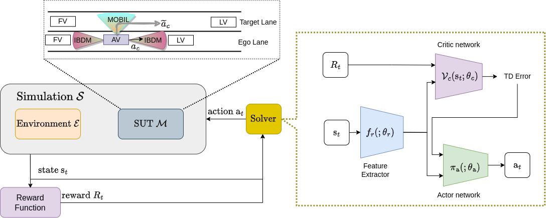
Figure 1: Our adaptive stress testing framework for finding crashed scenario in the highway. AV, FL and LV are notations for our autonomous vehicle (i.e., ego vehicle), following vehicle, and leading vehicle, respectively.

The design of our framework comprises three primary components, that is, the simulator $\mathcal{S}$, the reward function $R$, and the solver. The simulator evolves through different stages as the vehicle and other agents in the simulation environment interact. As the simulator transitions to a new state, it communicates any pertinent information regarding the state to the module associated with the AST reward function to obtain a reward value. Subsequently, the calculated reward is passed to the solver where the policy is updated, enabling it to generate the next environmental action. The overall architecture is presented in Figure 1 with the details being described below.

3.1 The simulator

The simulator $\mathcal{S}$ consists of an intelligent model for an autonomous vehicle $\mathcal{M}$ being used as a system under test (SUT) and the environment $\mathcal{E}$. This intelligent driving model ensures safe movements of the AV in the environment. We further define a set of goal states $E$ for the simulator, which represents the possible failure of the SUT. In this study, $E$ consists of all states that the ego vehicle likely to collide with other traffic participants. The goal of the RL solver is to update the state of the simulator $\mathcal{S}$ by generating environment actions that comply with the driving model and road rules while exploring the corner scenarios where collision is likely.

The AST technique is capable of managing a black-box or semi-black-box simulator that does not require the revelation of its complete internal states, and follows the following procedures:

• Init$(\mathcal{S})$: Reset the simulation to its starting state after the previous simulation epoch has terminated.

• Step$(\mathcal{S},\mathrm{a})$: Perform an action $\mathrm{a}_{t}$ at the time step $t$ and advance the simulator in time. Evaluate whether the new state of the simulation lies in the set of goal states $E$ and produce an indicator of this.

• IsTerminal$(\mathcal{S})$: Determine whether the current state belongs to the set of goal states $E$, or if the specified time limit has been exceeded.

The state of environment consists of all three vectors associated with the actions of the ego vehicle, environment actions by vehicles other than the ego vehicle, and the observations, that is,

$$\mathrm{s}_{env}=\left(\mathrm{a}_{ego},\mathrm{a}_{env},\mathrm{o}_{env}\right)$$ (1)

in which

• $\mathrm{a}_{ego}$ is the action of the ego vehicle which include $a^{ego}_{x}$ and $a^{ego}_{y}$ corresponding to the components of acceleration/deceleration in the longitudinal and latitudinal directions, respectively.

• $\mathrm{a}_{env}=\left(\mathrm{a}^{(1)}_{env},\mathrm{a}^{(2)}_{env},\ldots,\mathrm{a}^{(n)}_{env}\right)$, is the environment action at each time step associated with $n$ surrounding vehicles (other than the ego vehicle), and $\mathrm{a}^{(i)}_{env}$ is the high-level action for the $i$-th closest vehicle $(i=1,2,\ldots,n)$ that each vehicle’s action $\mathrm{a}^{(i)}_{env}$ can be one of several possible maneuvers, namely, left lane change, right lane change, acceleration, deceleration, or maintaining a constant speed.

• $\mathrm{o}_{env}=\left(\mathrm{o}^{(1)}_{env},\mathrm{o}^{(2)}_{env},\ldots,\mathrm{o}^{(n)}_{env}\right)$ is the observation that provides the kinematic information of both the ego vehicle and surrounding vehicles, where $\mathrm{o}^{(i)}_{env}$ represents the kinematic information of the $i$-th surrounding vehicle, which includes its positions $x^{(i)}$ and $y^{(i)}$, as well as its velocities $v_{x}^{(i)}$ and $v_{y}^{(i)}$, respectively, that is, $\mathrm{o}^{(i)}_{env}=(x^{(i)},y^{(i)},v_{x}^{(i)},v_{y}^{(i)})$ $(i=1,2,\ldots,n)$. Here, $v_{x}^{(i)}$ and $v_{y}^{(i)}$ (and $x^{(i)}$, $y^{(i)}$) refer to the longitudinal and latitudinal components, respectively, of the relative velocity (and relative position) between the ego vehicle and the $i$-th surrounding vehicle.

3.2 New reward function

We propose a novel reward function that is specifically designed to guide the simulation to identify scenarios in which a collision might occur in a highway environment. The proposed reward function overcomes the limitations in previous works, where only longitudinal trajectory is considered. More specifically, the primary limitation of existing rewards is the issue of sparse rewards. The multi-agent is only penalized if a collision is discovered when the state ends, i.e., at the end of which could be a long trajectory which leads to difficulty in learning how to find new cases with collisions.

Herein, we introduce a new reward function which further accounts for collisions along both longitudinal and lateral direction. Its aim is to to encourage the surrounding vehicle to move closely to the ego vehicle on the highway both horizontally and vertically, leading to a more diverse range of actions and potentially higher likelihood of a collision. To measure the collision probability of other vehicles against the ego vehicle, we utilize the notion of time-to-collision (TTC) (Saffarzadeh et al., 2013). In our study, at each time step, the highway environment may consist of up to six vehicles moving around the ego vehicle. They include the ones in front and rear, spanning three lanes: the ego lane, the left lane, and the right lane. The collision measurement of ego vehicle is calculated based on the collision probability of the ego vehicle with surrounding vehicles via comparing their TTC value with a predefined time threshold. Similar to the theory of using TTC time to determine cutting-in and cutting-out scenarios as proposed by Euro NCAP (NCAP, 2024; Edmonds et al., 2023), we check if the TTC time is less than the given threshold, the situation is then considered a collision where the collision probability is set to 1. Otherwise, the collision probability of a vehicle is the ratio between the TTC time of that vehicle to the ego vehicle and the TTC threshold shown in Equation 6. Finally, we calculate the ego vehicle collision probability by aggregating the collision probabilities of all surrounding vehicles into an overall score in Equation 5.

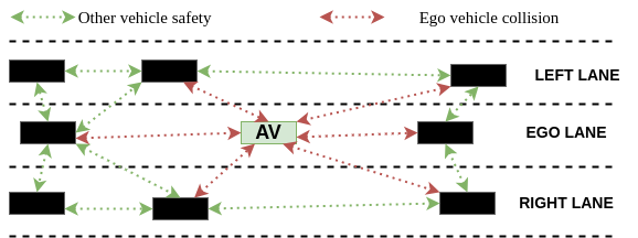
Figure 2: Illustration of interaction between vehicles with two components: other vehicle safety and ego vehicle collision.

Our reward function is defined based on two quantities: (i) the measurement of collision with the ego vehicle, being denoted as $\Phi_{collision}$, and (ii) the measurement of safety of vehicles surrounding the ego vehicle against other vehicles, being denoted as $\Psi_{safe}$. Figure 2 illustrates this two components and their impact on the movements of the ego vehicle and surrounding vehicles. The proposed reward function is defined as follows:

$$R({\mathrm{s}_{t}})= 0 \mathrm{s}_{t}\in E$$ (2)

$$R({\mathrm{s}_{t}})= -\alpha-\beta\min\limits_{\mathrm{v}_{q}\in\mathbf{N}(\mathrm{v}_{e})}t_{\text{TTC}}(\mathrm{v}_{e},\mathrm{v}_{q}) \mathrm{s}_{t}\notin E,t\geq T$$ (3)

$$R({\mathrm{s}_{t}})= \lambda\Phi_{\text{collision}}(\mathrm{s}_{t})+(1-\lambda)\Psi_{\text{safe}}(\mathrm{s}_{t}) \mathrm{s}_{t}\notin E,t<T$$ (4)

where $E$ is set of failure states (or collision scenarios) which is determined by intersecting two polygons covering vehicles similar to Leurent (2018); $\mathbf{N}(\mathrm{v}_{e})$ is the list of surrounding vehicles close to the ego vehicle $\mathrm{v}_{e}$ and $\mathbf{N}(\mathrm{v}_{i})$ is the set of surrounding vehicle close to the given vehicle $\mathrm{v}_{i}$; $t_{TTC}(\mathrm{v}_{p},\mathrm{v}_{q})$ is the time-to-collision between two vehicles $\mathrm{v}_{p}$ and $\mathrm{v}_{q}$, calculated based on Saffarzadeh et al. (2013); and $\alpha$ and $\beta$ in Equation 3 are parameters to penalize for failing to identify a collision (Mark et al., 2018; Corso et al., 2019). As we observe the maximum number of six vehicles closest to our ego vehicle mentioned earlier, the length of $\mathbf{N}(\mathrm{v}_{e})$ is always less than or equal to 6.

In our proposed reward function, we have introduced a weighting parameter $\lambda$ which has a value in the range of $[0,1]$ in Equation 4 for balancing between the safety measurement of surrounding vehicles (i.e. $\Psi$) and the collision measurement of the ego vehicle (i.e. $\Phi$). As explained earlier, the collision measurement of the ego vehicle can be expressed as:

$$\Phi(\mathrm{s}_{t})=\log\left(\frac{1}{\lVert\mathbf{N}(\mathrm{v}_{e})\rVert}\sum_{\mathrm{v}_{q}\in\mathbf{N}(\mathrm{v}_{e})}P_{collison}(\mathrm{s}_{t},\mathrm{v}_{q},\mathrm{v}_{e})\right)$$ (5)

where the collision probability $P_{collison}(\mathrm{s}_{t},\mathrm{v}_{p},\mathrm{v}_{q})$ of two vehicles $\mathrm{v}_{p}$ and $\mathrm{v}_{q}$ at a state $\mathrm{s}_{t}$ is calculated as below:

$$P_{collison}(\mathrm{s}_{t},\mathrm{v}_{p},\mathrm{v}_{q})=\begin{cases}1&t_{TTC}(\mathrm{v}_{p},\mathrm{v}_{q})\leq t_{\Delta}\\ t_{\Delta}/t_{TTC}(\mathrm{v}_{p},\mathrm{v}_{q})&\text{otherwise}\\ \end{cases}$$ (6)

Here, $t_{\Delta}$ is the time threshold where two vehicles are too close to each other and likely to collide.

At the same time, we are encouraging the surrounding vehicles to move safely without colliding with other vehicles. The measurement of safety movement of ego vehicle against other vehicles is given by

$$\Psi(\mathrm{s}_{t})=\frac{1}{\lVert\mathbf{N}_{surr}(\mathrm{v}_{e})\rVert}\sum_{\mathrm{v}_{q}\in\mathbf{N}_{surr}(\mathrm{v}_{e})}\Theta(\mathrm{s}_{t},\mathrm{v}_{q})$$ (7)

where $\mathbf{N}_{surr}(\mathrm{v}_{i})$ denotes the list of vehicles surrounding a given vehicle $\mathrm{v}_{i}$ within a distance $d$ of the vehicle $\mathrm{v}_{i}$ in any direction. The function $\Theta(\mathrm{s}_{t},\mathrm{v}_{i})$ represent the safety probability of a given vehicle $\mathrm{v}_{i}$ at the state $\mathrm{s}_{t}$, as below:

$$\Theta(\mathrm{s}_{t},\mathrm{v}_{i})=\log\left(\frac{1}{\lVert\mathbf{N}_{surr}(\mathrm{v}_{i})\rVert}\sum_{\mathrm{v}_{j}\in\mathbf{N}_{surr}(\mathrm{v}_{i})}P_{safe}(\mathrm{s}_{t},\mathrm{v}_{i},\mathrm{v}_{j})\right)$$ (8)

where:

$$P_{safe}(\mathrm{s}_{t},\mathrm{v}_{p},\mathrm{v}_{q})=\begin{cases}0&t_{TTC}(\mathrm{v}_{p},\mathrm{v}_{q})\leq t_{\Delta}\\ 1-t_{\Delta}/t_{TTC}(\mathrm{v}_{p},\mathrm{v}_{q})&\text{otherwise}\\ \end{cases}$$ (9)

We set the safety probability to be minimum, i.e. 0, when the TTC time is less than a threshold. We use the same threshold value $t_{\Delta}$ to determine both the safety probability and the collision probability.

3.3 The solver

We adopt Deep Q-Learning approach for the solver. Following Raffin et al. (2021), our network architecture is composed of three components, namely, the Feature extraction $f_{r}(;\theta_{r})$, the Critic network $\mathcal{V}_{c}(\mathrm{s}_{t};\theta_{c})$, and the Actor network $\pi_{\mathrm{a}}(;\theta_{\mathrm{a}})$. Its core component, i.e., the Feature extraction $f_{r}$ being parameterized by $\theta_{r}$, helps extract features from the environment state $\mathrm{s}_{t}$. In deep Q-learning, the function approximation can result in errors due to overvalued estimations. To address the issue, we parameterized critic network $\mathcal{V}_{c}$ by $\theta_{c}$ and estimate the error associated with Twin Delayed Deep Deterministic policy gradient (TD error) by taking the reward value $R_{t}$ and extracted features as input as in Fujimoto et al. (2018a). Following (Fujimoto et al., 2018b), the TD error is then used by the Actor network $\pi_{a}$ along with the extracted features from $f_{r}$ to approximate the environment action $\mathrm{a}_{t}$ as follows:

$$\text{TD Error}=R_{t+1}+\gamma\mathcal{V}_{c}(\mathrm{s}_{t+1};\theta_{c})-\mathcal{V}_{c}(\mathrm{s}_{t};\theta_{c})$$ (10)

where $\gamma$ is a discount factor ($0<\gamma<1$). In our implementation, we use a compact neural networks, which comprise of follows 256 fully connected hidden layers. To optimize the reinforcement learning policy, we utilize the proximal policy optimization (PPO) algorithm (Schulman et al., 2017), which were shown to be successful in finding failure trajectories with AST in other studies (Mark et al., 2021).

3.4 Our Intelligent Driving Model (uIDM)

We propose a comprehensive intelligent driving model referred to as unified Intelligent Driving Model (uIDM) accounting for both the complex longitudinal and latitudinal movements in the highway. We first build the uIDM based on the Intelligent Back-looking Driving Model (IBDM) to control the ego vehicle’s safe movement with both front and rear vehicles (Zi-wei et al., 2020). We then integrate into our uIDM the MOBIL model (Kesting, 2007) which enables the ego vehicle to safely change lanes while moving on the multi-lane highway. The new intelligent driving model can handle more sophisticated tasks in the highway environment due to its action capability as described below.

Longitudinal actions. uIDM is based on the assumption that vehicles on the highway are connected and thus information about all the front and rear vehicles surrounding the ego vehicle is available in real time. As a result, each vehicle’s acceleration might be adjusted to improve driver behavior and increase stability. The equations for determine the longitudinal acceleration or deceleration of a vehicle is expressed as follows:

$$a^{(i)}(t)=a^{(i)}_{acc}(t)+a^{(i)}_{dec}(t)$$ (11)

where

$$a^{(i)}_{acc}(t) =a^{(i)}_{max}\left(1-(\frac{v_{e}(t)}{v_{0}})^{\delta}\right)$$ (12)

$$a^{(i)}_{dec}(t) =-a^{(i)}_{max}\left(\frac{s^{*}\left(v_{e}(t),\Delta_{v_{e,l}(t)}\right)}{s_{e}(t)}-\epsilon\frac{s^{*}\left(v_{f}(t),\Delta_{v_{f,e}(t)}\right)}{s_{f}(t)}\right)^{2}$$ (13)

in which

$$\Delta_{v_{f,l}(t)} =v_{f}(t)-v_{l}(t)$$ (14)

$$s^{*}\left(v_{f}(t),\Delta_{v_{f,l}(t)}\right) =s_{0}+\mu v_{f}(t)+\frac{v_{f}(t)\Delta_{v_{f,e}(t)}}{2\sqrt{|a^{(i)}_{max}a^{(i)}_{min}|}}$$ (15)

In these equations, $v_{0}$ is the desired velocity; $s_{0}$ represents the minimal spatial separation between two neighboring vehicles in a highly congested traffic scenario; $\mu$ is desired time gap; $v_{e}(t),v_{f}(t),v_{l}(t)$ are the velocity of ego, following, leading vehicle respectively; $a^{(i)}_{max}$, $a^{(i)}_{min}$ are the maximum acceleration and deceleration, respectively; $\epsilon$ is the hyperparameter; and $\delta$ is the acceleration exponent that quantifies the degree to which the acceleration is influenced by the speed and gap.

Lateral actions.

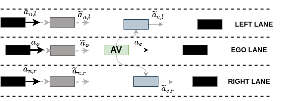
Figure 3: Lane change scenario with our uIDM which is similar to MOBIL (Kesting, 2007). The following vehicles in the left, ego, and right lanes each have their own accelerations, denoted as $a_{n,l},a_{o},a_{n,r}$ respectively. The ego vehicle, which is currently accelerating at a rate of $a_{e}$, has the option to switch to either the left lane or the right lane, with new accelerations of $\widetilde{a}_{e,l}$ and $\widetilde{a}_{e,r}$, respectively. After the ego vehicle changes lanes, the following vehicle can move with the new accelerations $\widetilde{a}_{n,l},\widetilde{a}_{o},\widetilde{a}_{n,r}$, respectively.

The MOBIL model is integrated to determine how safe it is to change lanes by considering the speeds of surrounding vehicles relative to the ego vehicle. Figure 3 illustrates how this algorithm considering dynamics of the vehicles to make the lane changing. Same as MOBIL, the decision-making process of uIDM has two steps. First, it makes sure that when the lane change happens the car behind it does not slow down too much which is formulated by the equation:

$$\widetilde{a}_{n}>a_{safe}$$ (16)

where $\widetilde{a}_{n}$ is the following (left or right) vehicle’s acceleration after changing lanes, and $a_{safe}$ is the ceiling threshold of acceleration when vehicle braking. Second, if the first safety criterion is met, uIDM continues to check the below condition before deciding to change lane Kesting (2007):

$$\underbrace{\widetilde{a}_{e}-a_{e}}_{\text{driver}}+\rho\left(\underbrace{\widetilde{a}_{n}-a_{n}}_{\text{next follower}}+\underbrace{\widetilde{a}_{o}-a_{o}}_{\text{previous follower}}\right)\geq\Delta a_{th}$$ (17)

where subscript $e$ denotes ego vehicle, while $o$ and $n$ stand for the previous and next followers after the lane change. The variable $a$ represents the vehicle’s acceleration before changing lane, and the variable $\widetilde{a}$ denote the vehicle’s acceleration after changing the lane. In the lane change action, the value of the variable $\rho$ is a politeness coefficient, and $\Delta a_{th}$ represents the acceleration gain required for performing a lane change.

4 Experiment

4.1 Settings

We describe the environmental setup and ways to evaluate the performance of our proposed approach. The highway environment is used to test the driving model, which consists multiple lanes where multiple vehicles move at different speeds. The highway-env (Leurent, 2018) package, introduced by OpenAI Gym, is used to train a vehicle controller whose goal is to gain a high speed while avoiding collisions with surrounding vehicles. The Stable-Baselines (Raffin et al., 2021) library is used to train Deep Q Network (DQN) for multi-agents controller.

4.2 Parameters settings and calibration

Parameters settings. To penalize the algorithm for failing to find a collision, the constants $\alpha$ and $\beta$ are set to 10,000 and 1000, respectively, according to previous works (Corso et al., 2019; Mark et al., 2018). Regarding surrounding vehicles, We set distance $d$ to 100m. For uIDM, we set $\epsilon$ to 0.4, $\mu$, $s_{0}$, $\delta$, and $a_{max}^{i},a_{min}^{i}$ to 1.5(s), 10(m), 4.0, 3.0(m/s2), and -5.0(m/s2) in longitudial control, $a_{safe}$ to -2.0(m/s2), $\rho$ to 0.0, and $\Delta a_{th}$ to 0.2(m/s2) for lateral control. In our experiment, 40 vehicles are driving on a four-lane highway. The speed limit on the road is 25 m/s (90 km/h). The vehicles are given a random starting speed of 25 m/s. The time-to-collision thresholds $t_{\Delta}$ are 1.5, 2, 2.5, 3, 3.5 seconds similar to the time-to-collision suggested by Euro Ncap (NCAP, 2024) to determine dangerous scenarios such as cutting-in, cutting out. The scenario runs for $4\times 10^{4}$ time steps. Our experiment is run on a machine os Ubuntu 20.04 and equipped with an NVIDIA GeForce P8 4 GB GPU and 24 GB RAM. The RL was trained with a batch size of 32, $T$ of 500 time steps, a discount factor $\gamma$ of 0.8, and a learning rate of $5\times 10^{-4}$. The neural network policy is composed of up of two hidden layers, each with 256 neural units.

Calibration. In our proposed reward function, the trade-off between two components is controlled primarily by the variable $\lambda$. To determine the appropriate $\lambda$, we design a series of experiments where $\lambda$ takes one of the values in the set {0, 0.1, 0.2, 0.3, 0.4, 0.5, 0.6, 0.7, 0.8, 0.9, 1}. Then, we use the statistics of California Autonomous Vehicles (CAV) crashes (Liu et al., 2021) as a ground truth to determine the value of $\lambda$ that best represents the crashes associated with autonomous vehicles in reality. Similar to CAV, we divide the types of crashes discovered by our framework into three groups: lane-change collisions, rear-end collisions, and other types.

Table 2: Comparison of framework performance with different values of $\lambda$ against the observations of crashes in California (Liu et al., 2021). Bold value indicate it is closest to CAV crashes item.

Source	Rear-end	Lane change	Other	$\mathcal{D}_{e}$
Ours., $\lambda=0.0$	70.63%	9.54%	19.83%	24.87%
Ours., $\lambda=0.1$	65.10%	10.53%	24.37%	20.61%
Ours., $\lambda=0.2$	67.33%	20.07%	12.60%	18.27%
Ours., $\lambda=0.3$	65.97%	16.62%	17.41%	17.12%
Ours., $\lambda=0.4$	60.62%	20.79%	18.59%	10.25%
Ours., $\lambda=0.5$	58.14%	21.82%	20.04%	7.41%
Ours., $\lambda=0.6$	60.53%	19.89%	19.58%	10.52%
Ours., $\lambda=0.7$	58.87%	20.18%	20.95%	8.98%
Ours., $\lambda=0.8$	56.21%	21.90%	21.89%	5.97%
Ours., $\lambda=0.9$	57.97%	21.23%	20.80%	7.61%
Ours., $\lambda=1.0$	58.56%	20.05%	21.39%	8.86%
CAV crashes	52.46%	26.47%	20.07%	-

Table 2 shows the detailed results of our frameworks’ collision group statistics for comparison with CAV observations. The results show that, with each collision type (rear-end, lane change, or other), our framework with $\lambda=0.8$ has a percentage of rear-end caused collisions that is closest to CAV crashes, and with $\lambda=0.5$, the percentage of lane-change caused collisions and other types are closest to CAV crashes, respectively. We measure the similarity of these triangle types using Euclidean distance, denoted $\mathcal{D}_{e}$ distance to better determine the most appropriate $\lambda$ in overall collisions types as below equation:

$$\mathcal{D}_{e}(\mathrm{q}^{\lambda},\mathrm{q}^{CAV})=\sqrt{(\mathrm{q}^{\lambda}_{r}-\mathrm{q}^{CAV}_{r})^{2}+(\mathrm{q}^{\lambda}_{l}-\mathrm{q}^{CAV}_{l})^{2}+(\mathrm{q}^{\lambda}_{o}-\mathrm{q}^{CAV}_{o})^{2}}$$ (18)

where $\mathrm{q}^{CAV}_{r},\mathrm{q}^{CAV}_{l},\mathrm{q}^{CAV}_{o}$, and $\mathrm{q}^{\lambda}_{r},\mathrm{q}^{\lambda}_{l},\mathrm{q}^{\lambda}_{o}$ are the statistics of rear-end, lane-change, other types of CAV crashes, and our method with a specific value of $\lambda$ as shown in Table 2. The Euclidean distance calculation results are also described in Table 2. With $\lambda=0.8$, our framework reaches the closest $\mathcal{D}_{e}$ distance to the statistics of observations. As a result, 0.8 is used as the selected value for all experiments.

5 Results and discussion

5.1 Quantitative results

We compare performance of our proposed method with the baseline of Log-Likelihood reward which was introduced by Mark et al. (2021). This reward function is defined as below as:

$$R_{LL}(\mathrm{s}_{t},\mathrm{a}_{t})=\begin{cases}0&s\in E\\ -\infty&s\notin E,t\geq T\\ \log(P(\mathrm{a}_{t}|\mathrm{s}_{t}))&s\notin E,t<T\end{cases}$$ (19)

We use the same set of critical states $E$ in both reward functions. Furthermore, we use the Log-Likelihood reward function to evaluate two systems under test: IDM and our proposed uIDM, separately, to evaluate the safety of our proposed driving model uIDM. These tests are referred to as LL-IDM and LL-uIDM, respectively. In particular, we analyze the performance of our framework with some driving model characteristics when a collision occurs such as vehicle maneuvers, collision type, vehicle speeds, and vehicle changing lanes and along with analysis of our proposed reward function.

5.1.1 Vehicle maneuvers

Table 3: Statistics of collision scenarios for both ego and other vehicle maneuvers leading to collisions. Ours.: our reward + uIDM. S, R, L are directions of ego vehicle going straight forward along ego lane, changing to the right lane, and shifting to the left lane, respectively. SV_LLC, SV_RLC, SV_CSK, SV_A, SV_D are five behaviors of crashed vehicle: change to the left lane, change to the right lane, keep constant speed, accelerate and decelerate.

Crashed vehicle Ego vehicle LL-IDM LL-uIDM Ours. ($\lambda=0.8$) Ours. ($\lambda=1$) Ours. ($\lambda=0$) S R L S R L S R L S R L S R L SV_LLC 126 - - 182 17 21 304 25 29 239 23 26 237 7 10 SV_RLC 165 - - 143 8 7 285 31 35 251 27 28 323 10 9 SV_CSK 284 - - 72 10 15 94 23 21 102 18 17 61 7 9 SV_A 259 - - 139 13 18 131 22 31 102 14 17 45 3 9 SV_D 23 - - 17 1 2 35 9 12 16 2 6 26 7 3 $\sum$ 1 action 857 - - 553 49 63 849 110 128 710 84 94 692 34 40 $\sum$ all actions 857 665 1087 888 766

Safe driving capability of new model. First, we analyze the vehicle maneuvers when a collision occurs. In the collision statistics described in Table 3, we combine three ego vehicle behaviors (go straight, turn left lane, turn right lane) with five crashed vehicle behaviors (change to the left lane, change to the right lane, keep a constant speed, accelerate, and decelerate). These results showed that the LL-IDM failed to identify any collisions when the ego vehicle changed to the left or right lane due to the fact that the IDM drives only in the longitudinal axis. In comparison to the IDM model, our proposed driving model (uIDM) using the Log-Likelihood reward, being denoted by LL-uIDM has less collisions (665) than the LL-IDM (857). Furthermore, the number of collisions of LL-uIDM in the four-last behaviors of a crashed vehicle is less than the number of collisions of LL-IDM. It indicates our proposed driving model, uIDM, is safer and, to some extent, more intelligent than the IDM model.

Contribution of new reward function. We compare our proposed reward function with the Log-Likelihood reward function through evaluating the LL-uDM and our reward with uIDM. Both reward functions are applied to guide the framework in identifying failure cases during testing of the same driving model, uIDM. Our framework identifies more crashed scenarios (1087) as compared to the Log-Likelihood reward function (665 crashed scenarios) (Table 3). Furthermore, our framework identifies a larger number and a more diverse set of diverse crashed scenarios than LL-uIDM in all of the behaviors of both the ego vehicle and the crashed vehicle. This result demonstrates that our framework with the novel proposed reward function outperforms the Log-Likelihood function (Mark et al., 2018; Corso et al., 2019) in identifying crashed scenarios.

Ablation study. To analyze the impact of two components in our proposed reward function on failure scenario discovery capabilities, we preliminarily add the results of our framework with $\lambda=0$ and $\lambda=1$, which correspond to the absence of collision measurement of ego vehicle, and safety measurement of surrounding vehicles, respectively, to Table 3. The results show that when one of these components is absent, the reward functions identify less crashed scenarios than when both are consisted of (i.e., $\lambda=0.8$). It indicates that it is essential to combine these two components in order to extend the longer trajectory of other vehicles while also potentially identifying more failure scenarios with the ego vehicle in need to develop a better stress testing framework.

5.1.2 Collision type

For this aspect, we categorize collisions that happen on ego vehicles into six types based on the location of the crashed vehicle at one time step immediately preceding the collision with ego vehicle, which is in the front, rear, or in the left, right, and same lane of ego vehicle. Specifically, they are referred to as crashed vehicle leading and coming from the left lane (FL), crashed vehicle leading in the ego lane (FE), crashed vehicle leading and coming from the right lane (FR), crashed vehicle following and coming from the left lane (RL), crashed vehicle following in the ego lane (RE), and crashed vehicle following and coming from the right lane (RR).

Table 4: Statistics of collision types over different value of $\lambda$ of our uIDM models in comparison with LL-IDM using our framework.

Method	Collision types
	FL	FE	FR	RL	RE	RR	Total
LL-IDM	10	152	5	33	436	29	665
Ours., $\lambda=1$	14	258	17	43	520	36	888
Ours., $\lambda=0$	2	160	2	36	541	25	766
Ours., $\lambda=0.8$	19	296	30	60	611	71	1087

Table 4 presents the detailed collision types results of LL-IDM and our framework with different components. Overall, all methods have a major number of collision in the RE or FE types. With LL-IDM, the identified collisions are heavily biased to the RE type and sparse in the rest types. Our approach helps detect more the FE collision type noticeably. Our framework achieves optimal balance and diversity in all six collision types through the incorporation of both components in our reward functions. This result demonstrates that our proposed method efficiently identifies an extensive variety of collision types in our experiments.

5.1.3 Characteristics of new reward functions

We do several analysis on the effectiveness of our proposed reward function in the AST framework. We conduct a comparative analysis between our proposed reward function and the Log-Likelihood reward function (Mark et al., 2018) through analyzing the velocity of the ego vehicle and the lane index in the scenario of a collision.

Vehicle speed.

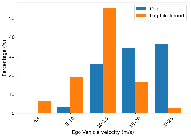
Figure 4: Comparison of our reward with the Log-Likelihood reward in percentage of crashed scenario on velocity range.

We analyze the velocity of the SUT immediately preceding the crash scenario. In our observations, we grouped speed into five ranges: 0-5, 5-10, 10-15, 15-20, and 20-25 (m/s). The column chart for percentage of collision by velocity range is shown in Figure 4. The figure shows that the Log-Likelihood reward for finding the crashed scenario is mostly distributed at speeds of 10-15 (m/s). The percentage of velocity in the ranges 5-10 and 15-20 is approximately the same, while the percentage of velocity in the range 20-25 is the smallest number. It could be because the Log-Likelihood controls the action of surrounding vehicles, allowing the SUT to avoid running at high speeds on the highway. In our proposed reward function, the crashed scenario occurred mostly in the highest velocity range, i.e. 20-25 (m/s), and the lower velocity range follows the percentage ranking. Since our framework is capable of capturing the crashes with higher speed, our proposed reward function becomes more reliable with real-world application.

Lane change patterns.

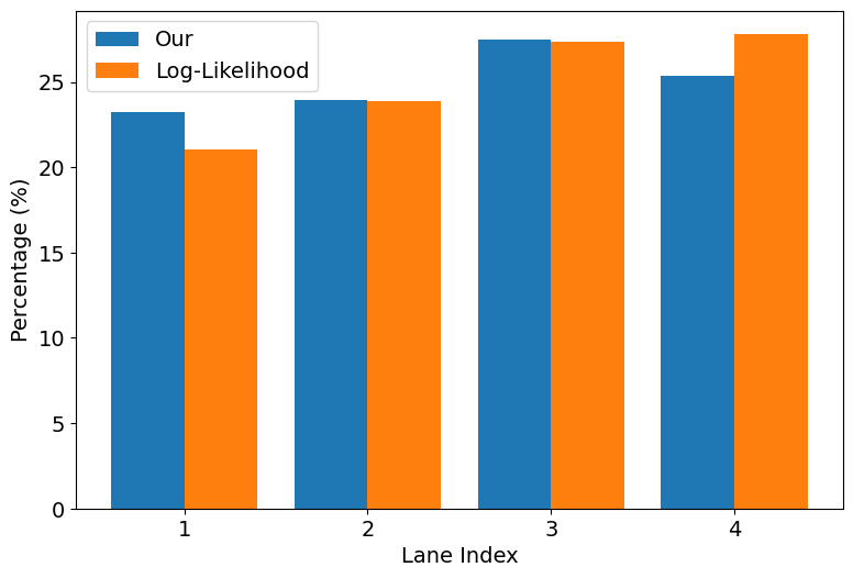
Figure 5: Comparison of our reward with the Log-Likelihood reward in percentage of crashed scenario on lane index.

By analyzing the lane change index, we can discover the behaviors of lane changes from one lane to another. This data is useful for comprehending the lateral movements of autonomous vehicles during on-road testing. To that end, we quantify the proportion of crashed scenarios in each lane index for various reward functions. The percentages of collisions by different lane indices are shown in Figure  5. For the second and third lanes, our framework achieves the same collision percentage as the log-likelihood reward framework. The collision percentage in the fourth lane, however, is higher than in the first, causing an imbalance in the remaining two lane indices. In general, the distribution of collision situations across each lane index in our framework is more evenly distributed.

Ablation study.

Table 5: Percentage of collision, betweek surrounding vehicles (Non-Ego) and only ego vehicle with surrounding vehicles (Ego) from different components in our proposed rewards. (Nums.: number of collision.)

Method	Collision
	Non-Ego		Ego		Total
	Nums.	%	Nums.	%	Nums.	%
Our., $\lambda=0$	11	1.44%	755	98.56%	766	100%
Our., $\lambda=1$	238	26.8%	650	73.2%	888	100%
Our., $\lambda=0.8$	223	22.01%	864	77.99%	1087	100%

We conduct an in-depth analysis to demonstrate the impact of each component on our proposed reward function. In this analysis, we observe a collision between a surrounding vehicle and surrounding vehicle. Our intuition is that if more collisions occur between surrounding vehicles, the surrounding vehicles will stop quickly in simulation, reducing the number of surrounding vehicles moving on the road and having a negative impact on the finding failure scenario of SUT. All collision scenarios revealed are divided into two types: (i) only one collision of the ego vehicle with the surrounding vehicle (Ego), and (ii) both collisions of the ego vehicle with the surrounding vehicle and collisions of the surrounding vehicle with the surrounding vehicle (Non-Ego). Table 5 presents the number of collisions and the percentage of each collision type in various components of our proposed reward functions. The results show that when only the safety of surrounding vehicles is considered (i.e. $\lambda=0$), the ratio of Non-Ego collision types is the smallest. However, because it also guides surrounding vehicles in moving safely, the number of collisions with the ego vehicle is the smallest (i.e. 766). When only collision measurement of ego vehicle is incorporated in our proposed reward function (that is, $\lambda=1$), the framework does not encourage the movement of surrounding vehicles, and the number of Non-Ego type collisions is highest. As the number of collision types increases, the surrounding vehicle may stop earlier than the length of the episode, resulting in a smaller number of crashes of the ego vehicle found at the end. Our reward function, which combines both of these components, can guide the framework to find a larger amount of collisions (i.e. 1087 versus 766 and 888). This demonstrates that combining collision measurement of ego vehicle with encouraging the movement of surrounding vehicles can result in more flexible and realistic results.

5.2 Qualitative analysis

LL-uIDM	Our., $\lambda=1$	Our., $\lambda=0$	Ours., $\lambda=0.8$
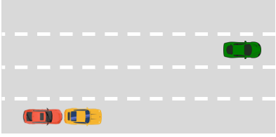
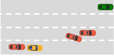
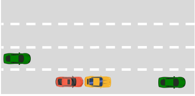
RE-a	RE-b	RE-c	RE-d
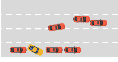
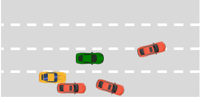
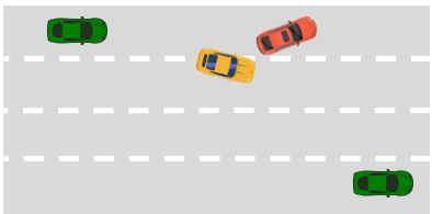
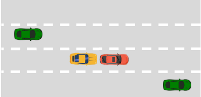
FE-a	FE-b	FE-c	FE-d
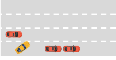
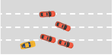
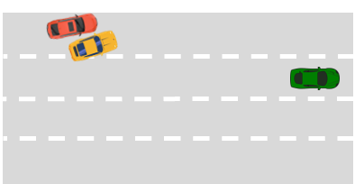
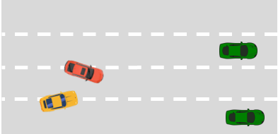
CLL-a	CLL-b	CLL-c	CLL-d
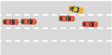
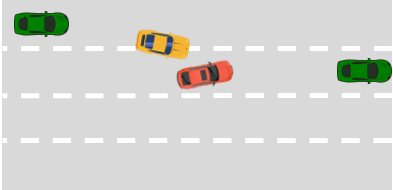
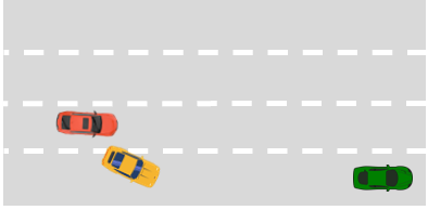
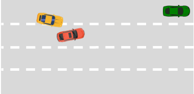
CRL-a	CRL-b	CRL-c	CRL-d
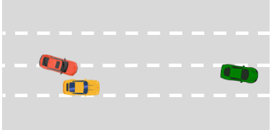
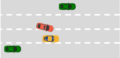
LVC-a	LVC-b	LVC-c	LVC-d
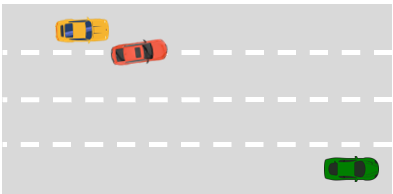
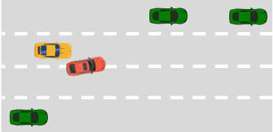
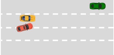
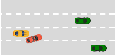
RVC-a	RVC-b	RVC-c	RVC-d

Figure 6: Examples of crashed scenarios sampled from various collision type for log-likelihood reward and our reward. Vehicles are moving from left to right. : Ego vehicle, : Crashed vehicle(s), and : Other vehicle(s). For the notations, RE: collision occurs in the rare of ego vehicle; FE: collision occurs in the front of ego vehicle; CLL: collision occurs when ego vehicle attempt changing to the left lane; CRL: collision occurs when ego vehicle attempt changing to the right lane; LVC: collision occurs when a vehicle is coming from the left side of ego vehicle; RVC: collision occurs when a vehicle is coming from the right side of ego vehicle.

We further conduct a qualitative analysis to compare the results generated by different reward formulations for diverse collision scenarios involving the ego vehicle, and then discuss the insights. We randomly sample examples of various collision types around the ego vehicle for this analysis. Figure 6 shows the crashed scenarios resulting from our proposed reward function with variety of $\lambda$ values, and Log-Likelihood reward function, respectively.

In case the crashed vehicles were following the ego vehicle and collided with it in the same lane (RE, Figure 6). Our model based on $\lambda=0.8$ had more moving vehicles on the road when the ego vehicle crashed as compared to the setting with $\lambda=0$. Furthermore, our framework with the combinations of two components (that is, $\lambda=0.8$), have more realistic crashed scenarios. For more detail, in the RE case, the ego vehicle actually tries to decrease speed to avoid collision with the close leading vehicle in the same lane, resulting in a collision with the following vehicle. However, in the examples of the Log-Likelihood method and our method with $\lambda=0$, there are no leading vehicles in front of the ego vehicle, causing the ego one to collide with the following accelerated vehicle. In the example of our method with $\lambda=1$, the ego vehicle accelerates to avoid a collision with the leading crashed vehicle, which leads to a collision with the following vehicle in the ego lane.

In case the crashed vehicles running in front of the ego vehicle in the same lane before the collision (RR, Figure 6), a sample Log-Likelihood depicts how the surrounding vehicles collides with each other, leading to a collision between the ego vehicle and the leading vehicle. In contrast, in our method with $\lambda=0.8$, two crashes occurs in the most right lane and the adjacent lane, resulting in a collision between the ego vehicle and the front vehicle. When $\lambda=0$, the ego vehicle may collide with a decelerated front vehicle. Meanwhile, in the example with $\lambda=1$, two front vehicles in the ego lane crash with each other, and in the adjacent lane, there is a moving vehicle, resulting in a collision between the ego vehicle and the front crashed vehicle.

In the scenario in which the collision occurs when ego vehicle attempt changing to the left lane (CLL, Figure 6), both the Log-Likelihood example and our method with $\lambda=1$ showed that surrounding vehicles collided with each other, and the ego vehicle needed to change to the left lane. However, in our method with $\lambda=0$, the ego vehicle attempted to change to the left lane to avoid the leading vehicle in the ego lane, but it should have had the option to change to the right lane. In the example of our method with $\lambda=0.8$, the ego vehicle attempted to change to the left lane to avoid a collision with a leading vehicle in the ego lane. However, at the same time, another vehicle changed lanes to the left lane to avoid a collision with its leading vehicle in the same lane, resulting in both vehicles changing lanes to the same lane, which led to a collision. This demonstrates that our method with $\lambda=0.8$ is arguably more realistic and critical than other methods.

In the context of the scenario in which collision occurs when ego vehicle attempt changing to the right lane (CLR, Figure 6), our method with $\lambda=0.8$ prompts the ego vehicle to change to the right lane to avoid collision with a vehicle ahead in the ego lane. However, at the same time, another vehicle attempts to change to the left lane to avoid colliding with a close vehicle in front. This results in a collision between the ego vehicle and the vehicle changing lanes. In contrast, in the example of the Log-Likelihood reward, the vehicles surrounding the ego vehicle collide with each other, and the sudden lane change of the ego vehicle is unexpected. On the other hand, our reward function with $\lambda=1$ is similar to the example with $\lambda=0.8$, but it includes a following vehicle of the ego vehicle, which may make the scenario more realistic than other examples.

Regarding the scenario in which the collision occurs when a vehicle is coming from the left side of ego vehicle (LVC, Figure 6), with our proposed reward function of $\lambda=0.8$, the ego vehicle is moving in a lane surrounded by two adjacent lanes with close-moving vehicles. Suddenly, a vehicle from the left lane changes its lane to the ego lane, resulting in a collision with the ego vehicle. Both the example of the Log-Likelihood reward and our reward function with individual components independently have a leading vehicle, but this vehicle is farther from the ego vehicle than in our reward function with $\lambda=0.8$. For this example, argue that our incorporated components may result in a more critical and realistic scenario.

Lastly, in the scenario in which the collision occurs when a vehicle is coming from the right side of ego vehicle (RVC, Figure 6), the example of the Log-Likelihood reward shows no leading vehicle when the collision occurs. The ego vehicle continues to move straight ahead in the ego lane while two adjacent lanes have moving vehicles. Suddenly, a vehicle from the right lane changes its lane to the ego lane, resulting in a collision with the ego vehicle. Again, our proposed reward function may discover more dangerous and realistic collision scenarios than the example with the Log-Likelihood reward.

6 Conclusion

In this paper, we proposed a novel AST framework and a novel reward function accounting for the ego vehicle’s collision avoidance capability while considering the safety impact of surrounding vehicles. The proposed framework was calibrated using the real-world accident statistics from California involving AVs. On top of that, we developed uIDM, a new intelligent driving model that integrates two well-known driving models to handle more complex tasks in the highway. Our experiments show that the proposed framework outperformed existing models and efficiently identified a wide range of crash scenarios, including lane changes, acceleration, and deceleration. The new framework and new driving model enabled use to gain important insights into the behaviours of AV in various complex driving scenarios. In future work, we will expand our stress testing method to involve more realistic scenarios such as highways with speed limits and traffic signs, as well as navigation intersections and u-turn driving.

References

- Beringhoff et al. (2022) Beringhoff, F., Greenyer, J., Roesener, C., Tichy, M., 2022. Thirty-one challenges in testing automated vehicles: Interviews with experts from industry and research, in: 2022 IEEE Intelligent Vehicles Symposium (IV), pp. 360–366. doi:10.1109/IV51971.2022.9827097.
- Browne et al. (2012) Browne, C.B., Powley, E., Whitehouse, D., Lucas, S.M., Cowling, P.I., Rohlfshagen, P., Tavener, S., Perez, D., Samothrakis, S., Colton, S., 2012. A survey of monte carlo tree search methods. IEEE Transactions on Computational Intelligence and AI in Games 4, 1–43. doi:10.1109/TCIAIG.2012.2186810.
- Corso et al. (2019) Corso, A., Du, P., Driggs-Campbell, K., Kochenderfer, M.J., 2019. Adaptive stress testing with reward augmentation for autonomous vehicle validatio. 2019 IEEE Intelligent Transportation Systems Conference (ITSC) , 163–168.
- Delecki et al. (2022) Delecki, H., Itkina, M., Lange, B., Senanayake, R., Kochenderfer, M.J., 2022. How do we fail? stress testing perception in autonomous vehicles, in: 2022 IEEE/RSJ International Conference on Intelligent Robots and Systems (IROS), IEEE. pp. 5139–5146.
- Edmonds et al. (2023) Edmonds, S., Castaing, P., van Ratingen, M., Gentilleau, M., Petit-Boulanger, C., 2023. Euro ncap rescue–tertiary safety assessment, in: 27th International Technical Conference on the Enhanced Safety of Vehicles (ESV) National Highway Traffic Safety Administration.
- Fan et al. (2020) Fan, J., Wang, Z., Xie, Y., Yang, Z., 2020. A theoretical analysis of deep q-learning, in: Proceedings of the 2nd Conference on Learning for Dynamics and Control, PMLR. pp. 486–489.
- Fujimoto et al. (2018a) Fujimoto, S., van Hoof, H., Meger, D., 2018a. Addressing function approximation error in actor-critic methods. arXiv:1802.09477.
- Fujimoto et al. (2018b) Fujimoto, S., van Hoof, H., Meger, D., 2018b. Addressing function approximation error in actor-critic methods, in: International Conference on Machine Learning.
- Hjelmeland et al. (2022) Hjelmeland, H.W., Eriksen, B.O.H., Mengshoel, O.J., Lekkas, A.M., 2022. Identification of failure modes in the collision avoidance system of an autonomous ferry using adaptive stress testing, pp. 470–477. doi:10.1016/j.ifacol.2022.10.472. 14th IFAC Conference on Control Applications in Marine Systems, Robotics, and Vehicles CAMS 2022.
- Hochreiter and Schmidhuber (1997) Hochreiter, S., Schmidhuber, J., 1997. Long short-term memory. Neural Computation 9, 1735–1780. doi:10.1162/neco.1997.9.8.1735.
- Kesting (2007) Kesting, A., 2007. Mobil : General lane-changing model for car-following models.
- Koren et al. (2020) Koren, M., Corso, A., Kochenderfer, M.J., 2020. The adaptive stress testing formulation. arXiv:2004.04293.
- Leurent (2018) Leurent, E., 2018. An environment for autonomous driving decision-making. https://github.com/eleurent/highway-env.
- Liu et al. (2021) Liu, Q., Wang, X., Wu, X., Glaser, Y., He, L., 2021. Crash comparison of autonomous and conventional vehicles using pre-crash scenario typology, p. 106281. doi:10.1016/j.aap.2021.106281.
- Lytskjold and Mengshoel (2023) Lytskjold, B., Mengshoel, O.J., 2023. Speeding up adaptive stress testing: Reinforcement learning using monte carlo tree search with neural networks and memoization, in: The 37th AAAI Conference on Artificial Intelligence.
- Mark et al. (2021) Mark, K., Ahmed, N., J., K.M., 2021. Finding failures in high-fidelity simulation using adaptive stress testing and the backward algorithm, IEEE Press. p. 5944–5949. doi:10.1109/IROS51168.2021.9636072.
- Mark and Mykel (2019) Mark, K., Mykel, K., 2019. Efficient autonomy validation in simulation with adaptive stress testing, in: 2019 IEEE Intelligent Transportation Systems Conference (ITSC), IEEE Press. p. 4178–4183. doi:10.1109/ITSC.2019.8917403.
- Mark et al. (2018) Mark, K., Saud, A., Ritchie, L., J., K.M., 2018. Adaptive stress testing for autonomous vehicles, in: 2018 IEEE Intelligent Vehicles Symposium (IV), pp. 1–7. doi:10.1109/IVS.2018.8500400.
- NCAP (2024) NCAP, E., 2024. Ad test and assessment protocol v2.0: Assisted driving highway and interurban assist systems. EUROpean New Car Assessment Program .