Density estimation for elliptic PDE with random input by preintegration and quasi-Monte Carlo methods

Abstract

In this paper, we apply quasi-Monte Carlo (QMC) methods with an initial preintegration step to estimate cumulative distribution functions and probability density functions in uncertainty quantification (UQ). The distribution and density functions correspond to a quantity of interest involving the solution to an elliptic partial differential equation (PDE) with a lognormally distributed coefficient and a normally distributed source term. There is extensive previous work on using QMC to compute expected values in UQ, which have proven very successful in tackling a range of different PDE problems. However, the use of QMC for density estimation applied to UQ problems will be explored here for the first time. Density estimation presents a more difficult challenge compared to computing the expected value due to discontinuities present in the integral formulations of both the distribution and density. Our strategy is to use preintegration to eliminate the discontinuity by integrating out a carefully selected random parameter, so that QMC can be used to approximate the remaining integral. First, we establish regularity results for the PDE quantity of interest that are required for smoothing by preintegration to be effective. We then show that an $N$-point lattice rule can be constructed for the integrands corresponding to the distribution and density, such that after preintegration the QMC error is of order $\mathcal{O}(N^{-1+\epsilon})$ for arbitrarily small $\epsilon>0$. This is the same rate achieved for computing the expected value of the quantity of interest. Numerical results are presented to reaffirm our theory.

Key words. uncertainty quantification, partial differential equations with random input, density estimation, quasi-Monte Carlo methods, preintegration, conditional sampling

MSC codes. 65D30, 65D32, 35J25, 62G07

1 Introduction

Quasi-Monte Carlo (QMC) methods have recently had great success in tackling high-dimensional problems in uncertainty quantification (UQ). While most of the research has focussed on computing the expected value of some quantity of interest involving the solution to a partial differential equation (PDE) with random input, see, e.g., [13, 16, 22, 23, 30, 35, 36], the task of computing other statistical objects for the quantity of interest has received less attention. In this paper, we introduce a method to approximate efficiently the cumulative distribution function (cdf) and probability density function (pdf) of the quantity of interest for an elliptic PDE with normally distributed random inputs.

Let $D\subset\mathbb{R}^{d}$, for $d=1,2$ or $3$, be a bounded convex domain and let $(\Omega,\mathcal{F},\pi)$ be a probability space. Consider the stochastic elliptic PDE

$$-\nabla\cdot(a({\boldsymbol{x}},\omega)\nabla u({\boldsymbol{x}},\omega))\, =\,\ell({\boldsymbol{x}},\omega)\,, {\boldsymbol{x}}\in D\,,$$ (1.1)

$$u({\boldsymbol{x}},\omega)\, =\,0\,, {\boldsymbol{x}}\in\partial D\,,$$

where the gradients are with respect to the physical variable ${\boldsymbol{x}}\in D$, and where $\omega\in\Omega$ is a random variable modelling the uncertainty in both the diffusion coefficient $a$ and the source term $\ell$. The random variable $\omega$ modelling the uncertainty will be specified formally below, but for now we note that it will typically be represented by a high number of parameters and that the randomness in the coefficient and the source term are assumed to be independent.

Our quantity of interest is a random variable $X\in\mathbb{R}$ given by a linear functional $\mathcal{G}$ of the solution to the PDE (1.1),

$$X\,=\,\mathcal{G}(u(\cdot,\omega))\,.$$ (1.2)

The cdf and pdf of $X$ are denoted by $F$ and $f$, respectively, and for $t\in[t_{0},t_{1}]\subset\mathbb{R}$, they can be formulated as the expected values

$$F(t)\, =\,\mathbb{P}[X\leq t]\,=\,\mathbb{E}_{\omega}[\operatorname{ind}(t-X)]\,=\,\int_{\Omega}\operatorname{ind}(t-\mathcal{G}(u(\cdot,\omega)))\,\mathrm{d}\pi(\omega),\quad\text{and}$$ (1.3)

$$f(t)\, =\,\mathbb{E}_{\omega}[\delta(t-X)]\,=\,\int_{\Omega}\delta(t-\mathcal{G}(u(\cdot,\omega)))\,\mathrm{d}\pi(\omega),$$ (1.4)

where $\operatorname{ind}$ is the indicator function and $\delta$ is the Dirac $\delta$ distribution, defined by

$$\delta(z)\,=\,0\quad\text{for all }z\neq 0\quad\text{and}\quad\int_{-\infty}^{\infty}\phi(y)\delta(y)\,\mathrm{d}y\,=\,\phi(0)$$

for all sufficiently smooth functions $\phi$.

The strategy for approximating the cdf $F$ and the pdf $f$ is to first use preintegration to smooth the discontinuity in each integrand, induced by the indicator and Dirac $\delta$ functions, respectively, and then to approximate the remaining integral by a QMC rule.

Motivated by the case where the diffusion coefficient and the source term are given by independent Gaussian random fields with separate Karhunen–Loéve expansions, we assume that $a$ is a lognormal coefficient and $\ell$ admits a finite affine series expansion. Let $s\in\mathbb{N}$ and let ${\boldsymbol{w}}=(w_{0},w_{1},\ldots,w_{s})\in\mathbb{R}^{s+1}$ be a vector of i.i.d. normally distributed random variables, i.e., $w_{i}\sim\mathrm{N}(0,1)$. We assume that the source term is given by

$$\ell({\boldsymbol{x}},\omega)\,\equiv\,\ell({\boldsymbol{x}},{\boldsymbol{w}})\,=\,\overline{\ell}({\boldsymbol{x}})+\sum_{i=0}^{s}w_{i}\,\ell_{i}({\boldsymbol{x}}),$$ (1.5)

where $\overline{\ell},\ell_{i}\in L^{2}(D)$ are known and deterministic. Similarly, let ${\boldsymbol{z}}=(z_{1},z_{2},\ldots,z_{s})\in\mathbb{R}^{s}$ be a vector of i.i.d. normally distributed random variables, i.e., $z_{j}\sim\mathrm{N}(0,1)$. We assume that the coefficient $a$ is given by

$$a({\boldsymbol{x}},\omega)\,\equiv\,a({\boldsymbol{x}},{\boldsymbol{z}})\,=\,\exp\bigg{(}\sum_{j=1}^{s}z_{j}\,a_{j}({\boldsymbol{x}})\bigg{)},$$ (1.6)

where $a_{j}\in L^{\infty}(D)$ are known and deterministic. In this formulation, the coefficient and the source term are independent and the random variable $\omega$ is given as a collection of normally distributed parameters $w_{0},w_{1},\ldots,w_{s}$ and $z_{1},\ldots,z_{s}$. Note that $w_{i}$ is indexed from $0$ to $s$ while $z_{j}$ is indexed from $1$ to $s$, for the sake of convenience when we discuss preintegration below.

To simplify the notation, we write the parameters in a single random vector ${\boldsymbol{y}}\in\mathbb{R}^{2s+1}$ with

$${\boldsymbol{y}}=(y_{0},y_{1},\ldots,y_{s},y_{s+1},\ldots,y_{2s})=(w_{0},w_{1},\ldots,w_{s},z_{1},\ldots,z_{s})=({\boldsymbol{w}},{\boldsymbol{z}})\in\mathbb{R}^{2s+1}.$$

We also write the PDE solution in terms of ${\boldsymbol{y}}$ as $u({\boldsymbol{x}},{\boldsymbol{y}})$ and then we write the quantity of interest (1.2) as

$$X=\mathcal{G}(u(\cdot,{\boldsymbol{y}})).$$ (1.7)

In this way, the expected values in the cdf (1.3) and pdf (1.4) can be written as $(2s+1)$-dimensional integrals with respect to a product Gaussian density,

$$F(t)\, =\,\int_{\mathbb{R}^{2s+1}}\operatorname{ind}(t-\mathcal{G}(u(\cdot,{\boldsymbol{y}})))\,\bigg{(}\prod_{i=0}^{2s}\rho(y_{i})\bigg{)}\,\mathrm{d}{\boldsymbol{y}},\quad\text{and}$$ (1.8)

$$f(t)\, =\,\int_{\mathbb{R}^{2s+1}}\delta(t-\mathcal{G}(u(\cdot,{\boldsymbol{y}})))\,\bigg{(}\prod_{i=0}^{2s}\rho(y_{i})\bigg{)}\,\mathrm{d}{\boldsymbol{y}}.$$ (1.9)

where $\rho(y)=\tfrac{1}{\sqrt{2\pi}}e^{-y^{2}/2}$ denotes the standard normal density.

The preintegration strategy is to first integrate out the variable $y_{0}=w_{0}$, so that evaluating the cdf (or pdf) becomes an integral of a (hopefully smooth) function over the remaining $2s$ variables ${\boldsymbol{y}}_{1:2s}=({\boldsymbol{w}}_{1:s},{\boldsymbol{z}})$. For convenience, later we will often abuse the notation and write ${\boldsymbol{y}}$ (or ${\boldsymbol{w}}$) to denote the vector without the initial variable $y_{0}$ (or $w_{0}$). There shall be no ambiguity from the context whether ${\boldsymbol{y}}$ (or ${\boldsymbol{w}}$) includes the variable $y_{0}$ (or $w_{0}$). We will make a critical assumption that

$$\ell_{0}({\boldsymbol{x}})>0\quad\mbox{for all}\quad{\boldsymbol{x}}\in D,$$

which ensures that the quantity of interest (1.7) is monotone with respect to the preintegration variable $y_{0}$, a property required for the preintegration theory (to be explained later in the article).

Preintegration is a special case of conditional Monte Carlo, or conditional sampling when more general quadrature rules are used, and as a numerical method it applies to more general non-smooth integrands than those in (1.8), (1.9). Conditional sampling is more general in that it allows one to condition on (or integrate out) partial information that is not restricted to a single variable. It has been used extensively as a smoothing and variance reduction technique in statistics and computational finance [1, 2, 4, 20, 21, 31, 42, 44, 47]. The smoothing effect of preintegration was analysed theoretically in [28], which builds upon the prior work [24, 25, 26]. More recently, the use of conditional sampling for density estimation was introduced in [43] and the special case of preintegration for density estimation was analysed in [19], with the latter paper [19] providing the setting followed here.

In practice, to evaluate the quantity of interest (1.7) the PDE (1.1) must be solved numerically by discretising the spatial domain, e.g., by a finite element method. Preintegration for the discrete problem requires a considerable amount of additional theory so will be discussed in depth in a subsequent paper [15]. However, for our numerical results we still use piecewise linear finite elements.

The structure of this paper is as follows: In Section 2, we introduce the background theory on smoothing by preintegration, including the function space setting, preintegration for density estimation and QMC methods for high-dimensional integration. In Section 3, we introduce the PDE with random input, along with our key assumptions and some important properties that will be used throughout the paper. Section 4 introduces our method for approximating the cdf and pdf of a quantity of interest coming from a PDE with random input. Then in Section 5, we verify that the PDE quantity of interest satisfies the conditions required for the smoothing by preintegration theory to apply. Following this, a full error analysis of our method is presented in Section 6. Section 7 presents numerical results that support the theoretical results from our error analysis and Section 8 provides concluding remarks.

2 Smoothing by preintegration

In this section we summarise the results from [19] for estimating the cdf and pdf of a real-valued random variable $X=\varphi({\boldsymbol{y}})$, which are given by

$$F(t)\, =\,\int_{\mathbb{R}^{2s+1}}\operatorname{ind}(t-\varphi({\boldsymbol{y}}))\,\bigg{(}\prod_{i=0}^{2s}\rho(y_{i})\bigg{)}\,\mathrm{d}{\boldsymbol{y}}\quad\text{and}$$ (2.1)

$$f(t)\, =\,\int_{\mathbb{R}^{2s+1}}\delta(t-\varphi({\boldsymbol{y}}))\,\bigg{(}\prod_{i=0}^{2s}\rho(y_{i})\bigg{)}\,\mathrm{d}{\boldsymbol{y}},$$ (2.2)

for a generic function $\varphi$ (ignoring the specific PDE problem for now), where the components $y_{i}$ are i.i.d. normally distributed random variables. The strategy is to preintegrate the non-smooth integrands in (2.1) and (2.2) with respect to $y_{0}$ to obtain functions in $2s$ variables ${\boldsymbol{y}}=(y_{1},\ldots,y_{2s})\in\mathbb{R}^{2s}$:

$$g_{\rm cdf}({\boldsymbol{y}}) \,\coloneqq\,\int_{-\infty}^{\infty}\operatorname{ind}(t-\varphi(y_{0},{\boldsymbol{y}}))\rho(y_{0})\,\mathrm{d}y_{0}\,,\quad\mbox{and}$$ (2.3)

$$g_{\rm pdf}({\boldsymbol{y}}) \,\coloneqq\,\int_{-\infty}^{\infty}\delta(t-\varphi(y_{0},{\boldsymbol{y}}))\rho(y_{0})\,\mathrm{d}y_{0}\,.$$ (2.4)

Then the cdf (2.1) and pdf (2.2) become $2s$-dimensional integrals of the functions $g_{\rm cdf}$ and $g_{\rm pdf}$,

$$F(t)=\int_{\mathbb{R}^{2s}}g_{\rm cdf}({\boldsymbol{y}})\bigg{(}\prod_{i=1}^{2s}\rho(y_{i})\bigg{)}\,\mathrm{d}{\boldsymbol{y}}\quad\mbox{and}\quad f(t)=\int_{\mathbb{R}^{2s}}g_{\rm pdf}({\boldsymbol{y}})\bigg{(}\prod_{i=1}^{2s}\rho(y_{i})\bigg{)}\,\mathrm{d}{\boldsymbol{y}}.$$ (2.5)

It is proved in [19] that $g_{\rm cdf}$ (2.3) and $g_{\rm pdf}$ (2.4) will be sufficiently smooth under appropriate conditions, and therefore the $2s$-dimensional integrals can be tackled successfully by QMC rules.

We start by introducing the function spaces needed to quantify smoothness and then summarise the results from [19].

2.1 Function spaces

We only define the $(2s+1)$-variate spaces, since the $2s$-variate spaces can be defined analogously by simply excluding the variable $y_{0}$.

Let $\mathbb{N}_{0}\coloneqq\{0,1,2,\ldots\}$. For $i=0,1,\ldots,2s$ and a multi-index ${\boldsymbol{\nu}}\in\mathbb{N}_{0}^{2s+1}$, let

$$\partial^{i}\coloneqq\frac{\partial}{\partial y_{i}}\qquad\mbox{and}\qquad\partial^{\boldsymbol{\nu}}\,\coloneqq\,\prod_{i=0}^{2s}\frac{\partial^{\nu_{i}}}{\partial y_{i}^{\nu_{i}}}$$

be the first-order derivative and the higher-order mixed derivative of order ${\boldsymbol{\nu}}$, respectively. This notation is used for derivatives with respect to ${\boldsymbol{w}}=(y_{0},y_{1},\ldots,y_{s})$ and ${\boldsymbol{z}}=(y_{s+1},y_{s+2},\ldots,y_{2s})$ as well. The ${\boldsymbol{\nu}}$th weak derivative of a function $\phi:\mathbb{R}^{2s+1}\to\mathbb{R}$ is the distribution $\partial^{\boldsymbol{\nu}}\phi$ that satisfies

$$\int_{\mathbb{R}^{2s+1}} \partial^{\boldsymbol{\nu}}\phi({\boldsymbol{y}})\,v({\boldsymbol{y}})\,\mathrm{d}{\boldsymbol{y}}\,=\,(-1)^{|{\boldsymbol{\nu}}|}\int_{\mathbb{R}^{2s+1}}\phi({\boldsymbol{y}})\,\partial^{\boldsymbol{\nu}}v({\boldsymbol{y}})\,\mathrm{d}{\boldsymbol{y}}\quad\text{for all }v\in C^{\infty}_{0}(\mathbb{R}^{2s+1}),$$

where $C^{\infty}_{0}(\mathbb{R}^{2s+1})$ is the space of infinitely differentiable functions with compact support.

For ${\boldsymbol{\nu}}\in\mathbb{N}_{0}^{2s+1}$, let $C^{\boldsymbol{\nu}}(\mathbb{R}^{2s+1})$ denote the space of functions with continuous mixed (classical) derivatives up to order ${\boldsymbol{\nu}}$:

$$C^{\boldsymbol{\nu}}(\mathbb{R}^{2s+1})\coloneqq\big{\{}\phi\in C(\mathbb{R}^{2s+1}):\partial^{{\boldsymbol{\eta}}}\phi\in C(\mathbb{R}^{2s+1})\text{ for all }{\boldsymbol{\eta}}\leq{\boldsymbol{\nu}}\}\,,$$

where $C(\mathbb{R}^{2s+1})$ denotes the space of continuous functions on $\mathbb{R}^{2s+1}$.

Moreover, for ${\boldsymbol{\nu}}\in\mathbb{N}_{0}^{2s+1}$ we define the Sobolev space of dominating mixed smoothness of order ${\boldsymbol{\nu}}$, denoted by $\mathcal{H}^{\boldsymbol{\nu}}_{2s+1}$, to be the space of locally integrable functions on $\mathbb{R}^{2s+1}$ such that the norm

$$\|\phi\|_{\mathcal{H}^{\boldsymbol{\nu}}_{2s+1}}^{2}\coloneqq\sum_{{\boldsymbol{\eta}}\leq{\boldsymbol{\nu}}}\frac{1}{\gamma_{\boldsymbol{\eta}}}\int_{\mathbb{R}^{2s+1}}|\partial^{{\boldsymbol{\eta}}}\phi({\boldsymbol{y}})|^{2}\,\boldsymbol{\psi}_{{\boldsymbol{\eta}}}({\boldsymbol{y}}_{\boldsymbol{\eta}})\,\boldsymbol{\rho}_{-{\boldsymbol{\eta}}}({\boldsymbol{y}}_{-{\boldsymbol{\eta}}})\,\mathrm{d}{\boldsymbol{y}}$$

is finite, where we introduced the shorthand notations

$$\gamma_{\boldsymbol{\eta}}\coloneqq\gamma_{\operatorname{supp}({\boldsymbol{\eta}})},\quad\boldsymbol{\psi}_{{\boldsymbol{\eta}}}({\boldsymbol{y}}_{\boldsymbol{\eta}})\coloneqq\prod_{i=0,\,\eta_{i}\neq 0}^{2s}\psi(y_{i})\quad\mbox{and}\quad\boldsymbol{\rho}_{-{\boldsymbol{\eta}}}({\boldsymbol{y}}_{-{\boldsymbol{\eta}}})\coloneqq\prod_{i=0,\,\eta_{i}=0}^{2s}\rho(y_{i}),$$

where $\operatorname{supp}({\boldsymbol{\eta}})\coloneqq\{i\in\{0:2s\}:\eta_{i}\neq 0\}$ is the set of indices for the nonzero components of ${\boldsymbol{\eta}}$. Here the behaviour of derivatives as $y_{i}\to\pm\infty$ is controlled by a strictly positive and integrable weight function $\psi:\mathbb{R}\to\mathbb{R}$. Also, here ${\boldsymbol{\gamma}}\coloneqq\{\gamma_{\mathrm{\mathfrak{u}}}>0:{\mathrm{\mathfrak{u}}}\subseteq\{0:2s\}\}$ is a collection of positive real numbers called weight parameters; they model the relative importance of different collections of variables, i.e., $\gamma_{\mathrm{\mathfrak{u}}}$ describes the relative importance of the collection of variables $(y_{i}:i\in{\mathrm{\mathfrak{u}}})$. We set $\gamma_{\emptyset}\coloneqq 1$. We define analogously the $2s$-variate Sobolev space $\mathcal{H}_{2s}^{\boldsymbol{\nu}}$, with variables indexed from $1$ to $2s$.

An important property of the Sobolev space of first-order dominating mixed smoothness, i.e., $\mathcal{H}^{{\boldsymbol{1}}}_{2s}$ with ${\boldsymbol{1}}\coloneqq(1,1,\ldots,1)$, is that it is equivalent to the unanchored space over the unbounded domain $\mathbb{R}^{2s}$ introduced in [38]. Explicitly, it was shown recently in [17] that if the weight function $\psi$ satisfies

$$\int_{-\infty}^{\infty}\frac{\Phi(y)(1-\Phi(y))}{\psi(y)}\,\mathrm{d}y\,<\,\infty,$$ (2.6)

where $\Phi$ is the cdf of $\rho$, then $\mathcal{H}^{{\boldsymbol{1}}}_{2s}$ and the unanchored space from [38] are equivalent. This equivalence is crucial as it immediately shows that the bounds on the QMC error from [38] also hold in $\mathcal{H}^{{\boldsymbol{1}}}_{2s}$. Examples of common pairings $(\rho,\psi)$ satisfying (2.6) can be found in [37, Table 3]. Note that for simplicity, $\psi_{i}^{2}$ in [37, 38], and also in [17, 19], is replaced here by a single $\psi$. The analysis in this paper will consider two types of weight functions, exponential and Gaussian. Exponential weight functions are of the form

$$\psi(y)\,=\,\exp(-2\,\mu\,|y|)\quad\text{for }\mu>0,$$ (2.7)

whereas Gaussian weight functions have the form

$$\psi(y)\,=\,\exp(-\mu\,y^{2})\quad\text{for }\mu\in(0,1/2).$$ (2.8)

Both choices of weight functions satisfy the condition (2.6).

2.2 Preintegration theory for density estimation

In this section we briefly summarise the theory on using smoothing by preintegration for density estimation from [19]. First, we make the following assumptions on $\varphi$ and $\rho$.

Assumption 1

For $s\geq 1$ and ${\boldsymbol{\nu}}\in\mathbb{N}_{0}^{2s}$, let $\varphi:\mathbb{R}^{2s+1}\to\mathbb{R}$ in (2.3) and (2.4) satisfy

1. $\partial^{0}\varphi(y_{0},{\boldsymbol{y}})>0$ for all $(y_{0},{\boldsymbol{y}})\in\mathbb{R}^{2s+1}$;

2. for each ${\boldsymbol{y}}\in\mathbb{R}^{2s}$, $\varphi(y_{0},{\boldsymbol{y}})\to\infty$ as $y_{0}\to\infty$; and

3. $\varphi\in\mathcal{H}^{(\nu_{0},{\boldsymbol{\nu}})}_{2s+1}\cap C^{(\nu_{0},{\boldsymbol{\nu}})}(\mathbb{R}^{2s+1})$, where $\nu_{0}\coloneqq|{\boldsymbol{\nu}}|+1$.

Additionally, suppose that $\rho\in C^{|{\boldsymbol{\nu}}|}(\mathbb{R})$.

Assumptions 1(a)–(b) imply that $\varphi$ is strictly increasing with respect to $y_{0}\in\mathbb{R}$ and also tends to $\infty$ as $y_{0}\to\infty$. Consequently, for fixed ${\boldsymbol{y}}\in\mathbb{R}^{2s}$ the discontinuity induced by the indicator function in (2.1) either occurs at a unique point $y_{0}$ or not at all. For a given $t\in[t_{0},t_{1}]$, we define the set of ${\boldsymbol{y}}\in\mathbb{R}^{2s}$ for which the discontinuity occurs by

$$U_{t}\,\coloneqq\,\{{\boldsymbol{y}}\in\mathbb{R}^{2s}\,:\,\varphi(y_{0},{\boldsymbol{y}})=t\mbox{ for some }y_{0}\in\mathbb{R}\}.$$ (2.9)

Then, the implicit function theorem [19, Theorem 3.1] states that if the set

$$R\coloneqq\big{\{}(t,{\boldsymbol{y}})\in(t_{0},t_{1})\times\mathbb{R}^{2s}:\varphi(y_{0},{\boldsymbol{y}})=t\text{ for some }y_{0}\in\mathbb{R}\big{\}}\,\subset\,[t_{0},t_{1}]\times\mathbb{R}^{2s}$$ (2.10)

is not empty, then there exists a unique function $\xi\in C^{(\nu_{0},{\boldsymbol{\nu}})}(\overline{R})$ satisfying

$$\varphi(\xi(t,{\boldsymbol{y}}),{\boldsymbol{y}})\,=\,t\qquad\mbox{for all}\quad(t,{\boldsymbol{y}})\in\overline{R}.$$ (2.11)

(Note that the set (2.10) was denoted by $V$ in [19].) Furthermore, for $(t,{\boldsymbol{y}})\in R$ the first-order derivatives of $\xi$ are given by

$$\partial^{i}\xi(t,{\boldsymbol{y}}) =-\frac{\partial^{i}\varphi(\xi(t,{\boldsymbol{y}}),{\boldsymbol{y}})}{\partial^{0}\varphi(\xi(t,{\boldsymbol{y}}),{\boldsymbol{y}})}\qquad\mbox{for all }i=1,\ldots,2s,\quad\text{and}$$

$$\frac{\partial}{\partial t}\xi(t,{\boldsymbol{y}}) =\frac{1}{\partial^{0}\varphi(\xi(t,{\boldsymbol{y}}),{\boldsymbol{y}})}.$$

The uniqueness of $\xi$ follows from the monotonicity condition Assumption 1(a). Similarly, because $\varphi(\cdot,{\boldsymbol{y}})$ is increasing, it follows from (2.11) that $\varphi(y_{0},{\boldsymbol{y}})<t$ if and only if $y_{0}<\xi(t,{\boldsymbol{y}})$, and so the preintegrated functions (2.3) and (2.4) can be written as

$$g_{\rm cdf}({\boldsymbol{y}})\,=\,\Phi(\xi(t,{\boldsymbol{y}}))\qquad\mbox{and}\qquad g_{\rm pdf}({\boldsymbol{y}})\,=\,\frac{\rho(\xi(t,{\boldsymbol{y}}))}{\partial^{0}\varphi(\xi(t,{\boldsymbol{y}}),{\boldsymbol{y}})},$$ (2.12)

for ${\boldsymbol{y}}\in U_{t}$, and both functions give $0$ if ${\boldsymbol{y}}\in\mathbb{R}^{2s}\setminus U_{t}$.

To establish the smoothness of $g_{\rm cdf}$ and $g_{\rm pdf}$, we need bounds on the typical functions that arise from taking mixed derivatives of $g_{\rm cdf}$ and $g_{\rm pdf}$ under the chain rule. The proofs of [19, Theorems 3.2 and 3.3] established that the mixed derivatives of $g_{\rm cdf}$ and $g_{\rm pdf}$ can be expressed as sums of typical functions of the form $h_{q,{\boldsymbol{\eta}}}(t,{\boldsymbol{y}})$ in (2.13) below. The proofs also obtained bounds on the total number of terms in those sums, which together with the constants $B_{q,{\boldsymbol{\eta}}}$ in (2.15) yield bounds on the $\mathcal{H}_{2s}^{{\boldsymbol{\nu}}}$-norm of $g_{\rm cdf}$ and $g_{\rm pdf}$.

Assumption 2

Let $s\geq 1$, ${\boldsymbol{\nu}}\in\mathbb{N}_{0}^{2s}$, $[t_{0},t_{1}]\subset\mathbb{R}$, and suppose that $\varphi$ and $\rho$ in (2.3) and (2.4) satisfy Assumption 1. Recall the definitions of $U_{t}$, $R$ and $\xi$ in (2.9), (2.10) and (2.11), respectively. Given $q\in\mathbb{N}_{0}$ and ${\boldsymbol{\eta}}\leq{\boldsymbol{\nu}}$ satisfying $|{\boldsymbol{\eta}}|+q\leq|{\boldsymbol{\nu}}|+1$, we consider functions $h_{q,{\boldsymbol{\eta}}}:\overline{R}\to\mathbb{R}$ of the form

$$\begin{cases}h_{q,{\boldsymbol{\eta}}}(t,{\boldsymbol{y}})=h_{q,{\boldsymbol{\eta}},(r,{\boldsymbol{\alpha}},\beta)}(t,{\boldsymbol{y}})\coloneqq\displaystyle\frac{(-1)^{r}\rho_{0}^{(\beta)}(\xi(t,{\boldsymbol{y}}))\,\prod_{\ell=1}^{r}\partial^{{\boldsymbol{\alpha}}_{\ell}}\varphi(\xi(t,{\boldsymbol{y}}),{\boldsymbol{y}})}{[\partial^{0}\varphi(\xi(t,{\boldsymbol{y}}),{\boldsymbol{y}})]^{r+q}},\\[11.38109pt] \mbox{with $r\in\mathbb{N}_{0}$, ${\boldsymbol{\alpha}}=({\boldsymbol{\alpha}}_{\ell})_{\ell=1}^{r}$, ${\boldsymbol{\alpha}}_{\ell}\in\mathbb{N}_{0}^{2s+1}\!\setminus\!\{{\boldsymbol{e}}_{0},{\boldsymbol{0}}\}$, $\beta\in\mathbb{N}_{0}$ satisfying}\\[2.84526pt] r\leq 2|{\boldsymbol{\eta}}|+q-1,\;\alpha_{\ell,0}\leq|{\boldsymbol{\eta}}|+q,\;\beta\leq|{\boldsymbol{\eta}}|+q-1,\;\beta{\boldsymbol{e}}_{0}+\displaystyle\sum_{\ell=1}^{r}{\boldsymbol{\alpha}}_{\ell}=(r+q-1,{\boldsymbol{\eta}}).\end{cases}$$ (2.13)

We assume that all such functions $h_{q,{\boldsymbol{\eta}}}$ satisfy

$$\lim_{{\boldsymbol{y}}\to\partial U_{t}}h_{q,{\boldsymbol{\eta}}}(t,{\boldsymbol{y}})=0\quad\text{for all }t\in[t_{0},t_{1}],$$ (2.14)

and there is a constant $B_{q,{\boldsymbol{\eta}}}$ such that

$$\sup_{t\in[t_{0},t_{1}]}\int_{U_{t}}|h_{q,{\boldsymbol{\eta}}}(t,{\boldsymbol{y}})|^{2}\,\boldsymbol{\psi}_{{\boldsymbol{\eta}}}({\boldsymbol{y}}_{\boldsymbol{\eta}})\,\boldsymbol{\rho}_{-{\boldsymbol{\eta}}}({\boldsymbol{y}}_{-{\boldsymbol{\eta}}})\,\mathrm{d}{\boldsymbol{y}}\leq B_{q,{\boldsymbol{\eta}}}\,<\,\infty.$$ (2.15)

The parameter ${\boldsymbol{\nu}}$ in Assumptions 1 and 2 determines the resulting smoothness of the preintegrated functions, while the parameter $q$ in Assumption 2 relates to whether the cdf or pdf is being considered. More precisely, under Assumption 1 and Assumption 2 for $q=0$ and all ${\boldsymbol{0}}\neq{\boldsymbol{\eta}}\leq{\boldsymbol{\nu}}$, the main result in [19, Theorem 3.2] states that, for $t\in[t_{0},t_{1}]$, the preintegrated function for the cdf satisfies

$$g_{\rm cdf}\in\mathcal{H}^{{\boldsymbol{\nu}}}_{2s}\cap C^{{\boldsymbol{\nu}}}(\mathbb{R}^{2s}),$$

with its $\mathcal{H}^{\boldsymbol{\nu}}_{2s}$-norm bounded uniformly in $t$,

$$\|g_{\rm cdf}\|_{\mathcal{H}^{\boldsymbol{\nu}}_{2s}}\leq\Bigg{(}1+\sum_{{\boldsymbol{0}}\neq{\boldsymbol{\eta}}\leq{\boldsymbol{\nu}}}\frac{\big{(}8^{|{\boldsymbol{\eta}}|-1}(|{\boldsymbol{\eta}}|-1)!\big{)}^{2}B_{0,{\boldsymbol{\eta}}}}{\gamma_{\boldsymbol{\eta}}}\Bigg{)}^{1/2}\,<\,\infty\,.$$ (2.16)

Similarly, under Assumption 1 and Assumption 2 for $q=1$ and all ${\boldsymbol{\eta}}\leq{\boldsymbol{\nu}}$, the result in [19, Theorem 3.3] states that, for $t\in[t_{0},t_{1}]$, the preintegrated function for the pdf satisfies

$$g_{\rm pdf}\in\mathcal{H}^{{\boldsymbol{\nu}}}_{2s}\cap C^{{\boldsymbol{\nu}}}(\mathbb{R}^{2s}),$$

with its $\mathcal{H}^{\boldsymbol{\nu}}_{2s}$-norm bounded uniformly in $t$,

$$\|g_{\rm pdf}\|_{\mathcal{H}^{\boldsymbol{\nu}}_{2s}}\leq\Bigg{(}\sum_{{\boldsymbol{\eta}}\leq{\boldsymbol{\nu}}}\frac{\big{(}8^{|{\boldsymbol{\eta}}|}|{\boldsymbol{\eta}}|!\big{)}^{2}B_{1,{\boldsymbol{\eta}}}}{\gamma_{\boldsymbol{\eta}}}\Bigg{)}^{1/2}\,<\,\infty\,.$$ (2.17)

Later in Section 5, we will obtain explicit constants $B_{q,{\boldsymbol{\eta}}}$ for the special case of the PDE quantity of interest described in the Introduction.

2.3 Quasi-Monte Carlo methods

Quasi-Monte Carlo (QMC) methods are a powerful class of equal-weight quadrature rules that have proven to be effective at approximating high-dimensional integrals. Originally designed for integration on the unit cube, they can also be used for integration on unbounded domains with respect to a product density $\boldsymbol{\rho}$, by mapping back to the unit cube using the inverse cdf transform. An $N$-point transformed QMC approximation to a $2s$-dimensional integral, as in (2.5), is given by

$$I_{2s}(g)\,\coloneqq\,\int_{\mathbb{R}^{2s}}g({\boldsymbol{y}})\boldsymbol{\rho}({\boldsymbol{y}})\,\mathrm{d}{\boldsymbol{y}}\,\approx\,\frac{1}{N}\sum_{n=0}^{N-1}g(\boldsymbol{\Phi}^{-1}({\boldsymbol{q}}_{n}))\,\eqqcolon\,Q_{2s,N}(g)\,,$$ (2.18)

where the inverse cdf $\boldsymbol{\Phi}^{-1}$ is applied componentwise to map the QMC points, $\{{\boldsymbol{q}}_{n}\}_{n=0}^{N-1}$, from the unit cube to $\mathbb{R}^{2s}$. For further details on QMC see, e.g., [10].

In this paper, we use a simple class of randomised QMC methods called randomly shifted lattice rules. For a generating vector $\boldsymbol{{\boldsymbol{z}}}_{\mathrm{gen}}\in\mathbb{N}^{2s}$ and a uniformly distributed random shift ${\boldsymbol{\Delta}}\in[0,1)^{2s}$, the randomly shifted lattice points are given by

$${\boldsymbol{q}}_{n}\,\coloneqq\,\bigg{\{}\frac{n\boldsymbol{{\boldsymbol{z}}}_{\mathrm{gen}}}{N}+{\boldsymbol{\Delta}}\bigg{\}}\quad\text{for }n=0,1,\ldots,N-1,$$

where $\{\cdot\}$ denotes taking the fractional part componentwise.

Good generating vectors can be constructed using the component-by-component (CBC) construction. For the unbounded setting as in (2.18), the CBC construction was developed in [38]. Theorem 8 in [38] shows that under certain conditions on the weight function $\psi$, the root-mean-square error (RMSE) of a CBC-generated randomly shifted lattice rule achieves close to $\mathcal{O}(1/N)$ convergence. Below we present their main result adapted for $\mathcal{H}_{2s}^{\boldsymbol{1}}$ for the choice of exponential and Gaussian weight functions (see also [17]).

Theorem 1

For $s,N\in\mathbb{N}$, let $\psi$ be either an exponential or Gaussian weight function and let $g\in\mathcal{H}^{{\boldsymbol{1}}}_{2s}$ with weight parameters ${\boldsymbol{\gamma}}=(\gamma_{{\boldsymbol{\eta}}})_{{\boldsymbol{\eta}}\leq{\boldsymbol{1}}}$. Then a randomly shifted lattice rule with $N$ points in $2s$ dimensions can be constructed using a CBC algorithm such that, for $\epsilon\in(0,1/2]$ depending on $\psi$, the RMSE satisfies

$$\sqrt{\mathbb{E}_{\boldsymbol{\Delta}}\big{[}|I_{2s}(g)-Q_{2s,N}(g)|^{2}\big{]}}\leq\bigg{(}\frac{1}{\phi_{\rm{tot}}(N)}\sum_{{\boldsymbol{0}}\neq{\boldsymbol{\eta}}\leq{\boldsymbol{1}}}\gamma_{\boldsymbol{\eta}}^{1/(2(1-\epsilon))}\,\varrho(\epsilon)^{|{\boldsymbol{\eta}}|}\bigg{)}^{1-\epsilon}\|g\|_{\mathcal{H}^{\boldsymbol{1}}_{2s}}\,,$$ (2.19)

where $\phi_{\mathrm{tot}}$ is the Euler totient function and $\varrho$ also depends on $\psi$.

For an exponential weight function, $\psi(y)=e^{-2\mu|y|}$ with $\mu>0$, the bound (2.19) holds for all $\epsilon\in(0,1/2]$ with

$$\varrho(\epsilon)\,=\,2\bigg{(}\frac{4\sqrt{2\pi}\exp(2\mu^{2}/\epsilon)}{\pi^{2-\epsilon}(2-\epsilon)\epsilon}\bigg{)}^{1/(2(1-\epsilon))}\,\zeta\bigg{(}\frac{1-\epsilon/2}{1-\epsilon}\bigg{)}\,,$$ (2.20)

whereas for a Gaussian weight function, $\psi(y)=e^{-\mu y^{2}}$ with $\mu\in(0,1/2)$, the bound (2.19) holds for all $\epsilon\in(\mu,1/2]$ with

$$\varrho(\epsilon)\,=\,2\bigg{(}\dfrac{\sqrt{2\pi}}{\pi^{2-2\mu}(1-\mu)\mu}\bigg{)}^{1/(2(1-\epsilon))}\,\zeta\bigg{(}\frac{1-\mu}{1-\epsilon}\bigg{)}\,.$$ (2.21)

Proof.

Theorem 8 in [38] gives for all $\lambda\in(1/(2r_{2}),1]$,

$$\sqrt{\mathbb{E}_{\boldsymbol{\Delta}}\big{[}|I_{2s}(g)-Q_{2s,N}(g)|^{2}\big{]}}\leq\bigg{(}\frac{1}{\phi_{\rm{tot}}(N)}\sum_{{\boldsymbol{0}}\neq{\boldsymbol{\eta}}\leq{\boldsymbol{1}}}\gamma_{\boldsymbol{\eta}}^{\lambda}\,[2C_{2}^{\lambda}\zeta(2r_{2}\lambda)]^{|{\boldsymbol{\eta}}|}\bigg{)}^{1/(2\lambda)}\|g\|_{\mathcal{H}^{\boldsymbol{1}}_{2s}}\,,$$ (2.22)

where $r_{2}\in(0,1)$ and $C_{2}$ depend on $\psi$. Note that we have also used the equivalence of the unanchored space from [38] and $\mathcal{H}^{\boldsymbol{1}}_{2s}$ from [17] to write this in terms of $\mathcal{H}^{\boldsymbol{1}}_{2s}$.

Following Example 5 in [37] (with parameters $\nu=1$ and $\alpha=2/\mu$), for an exponential weight function we have for any $\delta\in(0,1/2)$,

$$C_{2}\,=\,\dfrac{\sqrt{2\pi}\exp(\mu^{2}/\delta)}{\pi^{2-2\delta}(1-\delta)\delta}\quad\text{and}\quad r_{2}=1-\delta.$$

The result (2.19) with (2.20) follows by letting $\varrho(\epsilon)=2C_{2}^{\lambda}\zeta(2r_{2}\lambda)$ with $\delta=\epsilon/2$ and $\lambda=1/(2(1-\epsilon))$, noting that $\lambda=1/(2(1-\epsilon))>1/(2r_{2})=1/(2(1-\epsilon/2))$.

For a Gaussian weight function, Example 4 in [37] (with $\nu=1$ and $\alpha=1/\mu$) gives

$$C_{2}=\dfrac{\sqrt{2\pi}}{\pi^{2-2\mu}(1-\mu)\mu}\quad\text{and}\quad r_{2}=1-\mu,$$

In this case, the result (2.19) with (2.21) follows by letting $\varrho(\epsilon)=2C_{2}^{\lambda}\zeta(2r_{2}\lambda)$ and $\lambda=1/(2(1-\epsilon))$ for $\epsilon\in(\mu,1/2]$, noting that $\lambda=1/(2(1-\epsilon))>1/(2r_{2})=1/(2(1-\mu))$ since $\epsilon>\mu$. ∎

To ensure that the preintegrated functions $g_{\mathrm{cdf}}$ and $g_{\mathrm{pdf}}$ as in (2.12) belong to $\mathcal{H}^{{\boldsymbol{1}}}_{2s}$, and hence achieve the QMC error bound (2.19), we require that Assumptions 1 and 2 hold for ${\boldsymbol{\nu}}={\boldsymbol{1}}$, which will be verified in Section 5.

3 PDE with random input

In this section, we introduce the necessary background material on PDE with random (specifically, i.i.d. normally distributed) inputs. First, we start with the following notation. Let $V\coloneqq H_{0}^{1}(D)$ denote the first-order Sobolev space with vanishing boundary trace, equipped with the norm $\|v\|_{V}\coloneqq\|\nabla v\|_{L^{2}(D)}$, and denote the dual space by $V^{*}\coloneqq H^{-1}(D)$. We will also use the notation $\langle\cdot,\cdot\rangle$ to denote the $L^{2}(D)$ inner product, which can be extended continuously to a duality paring on $V^{*}\times V$. Similarly, $W^{k,p}(D)$ denotes the usual Sobolev space of smoothness $k\in\mathbb{N}$ and integrability $1\leq p\leq\infty$, with the Hilbert spaces ($p=2$) denoted by $H^{k}(D)\coloneqq W^{k,2}(D)$.

Next, we make the following assumptions on the physical domain $D$, the coefficient $a$ and the right hand side $\ell$, which will ensure that the variational form of PDE (1.1) is well posed.

Assumption 3

Let $d\in\{1,2,3\}$. For the PDE problem (1.1) we assume that

1. $D\subset\mathbb{R}^{d}$ is a bounded convex domain, and furthermore, $D$ is a strictly convex polygon when $d=2$, and $D$ has a $C^{2}$ boundary when $d=3$;

2. for ${\boldsymbol{z}}\in\mathbb{R}^{s}$, $a(\cdot,{\boldsymbol{z}})\in W^{1,\infty}(D)$ is of the form (1.6) with $a_{j}\in W^{1,\infty}(D)$ and $z_{j}\sim\mathrm{N}(0,1)$ for $j=1,2,\ldots,s$;

3. for ${\boldsymbol{w}}\in\mathbb{R}^{s+1}$, $\ell(\cdot,{\boldsymbol{w}})\in V^{*}$ is of the form (1.5) with $\overline{\ell}$, $\ell_{i}\in V^{*}$ and $w_{i}\sim\mathrm{N}(0,1)$ for $i=0,1,2,\ldots,s$; and

4. $\ell_{0}\in L^{\infty}(D)$ with $\ell_{0,\inf}\coloneqq\inf_{{\boldsymbol{x}}\in D}\ell_{0}({\boldsymbol{x}})>0$.

Here $W^{1,\infty}(D)$, the Sobolev space of functions with essentially bounded weak derivatives on $D$, is equipped with the norm $\|v\|_{W^{1,\infty}(D)}\coloneqq\max\{\|v\|_{L^{\infty}(D)},\|\nabla v\|_{L^{\infty}(D)}\}$.

Assumption 3(b) implies that for ${\boldsymbol{z}}\in\mathbb{R}^{s}$ there exists $a_{\mathrm{min}}({\boldsymbol{z}})<a_{\mathrm{max}}({\boldsymbol{z}})$ such that

$$a_{\mathrm{min}}({\boldsymbol{z}})\,\leq\,a({\boldsymbol{x}},{\boldsymbol{z}})\,\leq\,a_{\mathrm{max}}({\boldsymbol{z}})\quad\text{for all }{\boldsymbol{x}}\in D.$$ (3.1)

Furthermore, $a_{\mathrm{max}},1/a_{\mathrm{min}}\in L_{\boldsymbol{\rho}}^{p}(\mathbb{R}^{s})$ for all $1\leq p<\infty$, where $L_{\boldsymbol{\rho}}^{p}(\mathbb{R}^{s})$ denotes the space of $p$-integrable functions on $\mathbb{R}^{s}$ with respect to the product normal density $\boldsymbol{\rho}$.

The smoothness of $u(\cdot,{\boldsymbol{y}})$ will be governed by further regularity of $\overline{\ell},\ \ell_{i}$ beyond $V^{*}$. The extra condition on $\ell_{0}$ in Assumption 3(d) is required to ensure that the monotonicity condition for preintegration (cf. Assumption 1(a)) is satisfied, see Section 5.1.

3.1 Parametric variational form

In the usual way, the variational formulation is obtained by multiplying the PDE (1.1) by a test function $v\in V$ then using Green’s formula to integrate by parts with respect to ${\boldsymbol{x}}$, giving

$$\int_{D}a({\boldsymbol{x}},{\boldsymbol{z}})\,\nabla u({\boldsymbol{x}},{\boldsymbol{y}})\cdot\nabla v({\boldsymbol{x}})\,\mathrm{d}{\boldsymbol{x}}=\int_{D}\ell({\boldsymbol{x}},{\boldsymbol{w}})\,v({\boldsymbol{x}})\,\mathrm{d}{\boldsymbol{x}},$$ (3.2)

for some parameter

$${\boldsymbol{y}}=(y_{0},y_{1},\ldots,y_{s},y_{s+1},\ldots,y_{2s})=(w_{0},w_{1},\ldots,w_{s},z_{1},\ldots,z_{s})=({\boldsymbol{w}},{\boldsymbol{z}})\in\mathbb{R}^{2s+1}.$$

For ${\boldsymbol{z}}\in\mathbb{R}^{s}$, define also the parametric bilinear form $\mathcal{A}({\boldsymbol{z}};\cdot,\cdot):V\times V\to\mathbb{R}$ by

$$\mathcal{A}({\boldsymbol{z}};v,v^{\prime})\,\coloneqq\,\int_{D}a({\boldsymbol{x}},{\boldsymbol{z}})\,\nabla v({\boldsymbol{x}})\cdot\nabla v^{\prime}({\boldsymbol{x}})\,\mathrm{d}{\boldsymbol{x}}\quad\text{ for }v,v^{\prime}\in V.$$ (3.3)

For any particular ${\boldsymbol{y}}\in\mathbb{R}^{2s+1}$, the variational formulation of (1.1) is: find $u(\cdot,{\boldsymbol{y}})\in V$ such that

$$\mathcal{A}({\boldsymbol{z}};u(\cdot,{\boldsymbol{y}}),v)=\langle\ell(\cdot,{\boldsymbol{w}}),v\rangle\quad\text{for all }v\in V.$$ (3.4)

The condition (3.1) on the coefficient $a(\cdot,{\boldsymbol{z}})$ implies that the bilinear form $\mathcal{A}(z;\cdot,\cdot)$ is coercive and continuous, i.e., for any given ${\boldsymbol{z}}\in\mathbb{R}^{s}$ and all $v,v^{\prime}\in V$

$$\mathcal{A}({\boldsymbol{z}};v,v)\,\geq\,a_{\mathrm{min}}({\boldsymbol{z}})\|v\|^{2}_{V}\qquad\text{and}\qquad|\mathcal{A}({\boldsymbol{z}};v,v^{\prime})|\,\leq\,a_{\mathrm{max}}({\boldsymbol{z}})\|v\|_{V}\|v^{\prime}\|_{V}.$$

The Lax–Milgram Lemma then implies that the variational problem (3.4) admits a unique solution $u(\cdot,{\boldsymbol{y}})\in V$, with the following upper bound

$$\|u(\cdot,{\boldsymbol{y}})\|_{V}\,\leq\,\frac{\|\ell(\cdot,{\boldsymbol{w}})\|_{V^{*}}}{a_{\mathrm{min}}({\boldsymbol{z}})}\,\leq\,\frac{1}{a_{\mathrm{min}}({\boldsymbol{z}})}\bigg{(}\|\overline{\ell}\|_{V^{*}}+\sum_{i=0}^{s}|w_{i}|\,\|\ell_{i}\|_{V^{*}}\bigg{)},$$ (3.5)

where in the second inequality we have used the specific form (1.5) of $\ell(\cdot,{\boldsymbol{w}})$ and the triangle inequality. Similarly, for $\mathcal{G}\in V^{*}$, the quantity of interest (1.7) is bounded by

$$|\mathcal{G}(u(\cdot,{\boldsymbol{y}}))|\,\leq\,\|\mathcal{G}\|_{V^{*}}\|u(\cdot,{\boldsymbol{y}})\|_{V}\,\leq\,\frac{\|\mathcal{G}\|_{V^{*}}\|\ell(\cdot,{\boldsymbol{w}})\|_{V^{*}}}{a_{\mathrm{min}}({\boldsymbol{z}})}\,.$$ (3.6)

Due to linear structure of the source term (1.5), the solution $u(\cdot,{\boldsymbol{y}})\in V$ of (3.4) can be written as a sum of $s+1$ solutions,

$$u({\boldsymbol{x}},{\boldsymbol{y}})\,=\,\overline{u}({\boldsymbol{x}},{\boldsymbol{z}})+\sum_{i=0}^{s}w_{i}\,u_{i}({\boldsymbol{x}},{\boldsymbol{z}}),$$ (3.7)

where $\overline{u}(\cdot,{\boldsymbol{z}})\in V$ and $u_{i}(\cdot,{\boldsymbol{z}})\in V$ denote the solutions to (3.4) with source terms $\overline{\ell}\in V^{*}$ and $\ell_{i}\in V^{*}$, respectively, and they are independent of ${\boldsymbol{w}}$. Again the Lax–Milgram Lemma ensures that the solutions $\overline{u}(\cdot,{\boldsymbol{z}})\in V$ and $u_{i}(\cdot,{\boldsymbol{z}})\in V$ are unique. In addition, both of the a priori bounds (3.5) and (3.6) also hold for $\overline{u}(\cdot,{\boldsymbol{z}}),\ u_{i}(\cdot,{\boldsymbol{z}})$ but with $\overline{\ell},\ \ell_{i}$ on the right, respectively. Similarly, the quantity of interest (1.7) can be expressed as

$$\mathcal{G}(u(\cdot,{\boldsymbol{y}}))\,=\,\mathcal{G}(\overline{u}(\cdot,{\boldsymbol{z}}))+\sum_{i=0}^{s}w_{i}\ \mathcal{G}(u_{i}(\cdot,{\boldsymbol{z}})).$$ (3.8)

3.2 Parametric regularity

To apply the preintegration theory from Section 2.2, as well as the QMC theory from Section 2.3, to this PDE problem, we require that the solution $u$ is sufficiently regular with respect to the parameter ${\boldsymbol{y}}$. Parametric regularity results for an arbitrary right-hand side are given in, e.g., [22], which can easily be adapted to our setting as in the following theorem.

For readability, we adopt the notation

$$b_{j}\,\coloneqq\,\|a_{j}\|_{L^{\infty}(D)},\quad\overline{c}\,\coloneqq\,\|\overline{\ell}\|_{V^{*}}\quad\text{and}\quad c_{i}\,\coloneqq\,\|\ell_{i}\|_{V^{*}}\,.$$ (3.9)

We also split the order ${\boldsymbol{\nu}}\in\mathbb{N}_{0}^{2s+1}$ for the derivative with respect to ${\boldsymbol{y}}=({\boldsymbol{w}},{\boldsymbol{z}})$ by writing ${\boldsymbol{\nu}}=({\boldsymbol{\nu}}_{\boldsymbol{w}},{\boldsymbol{\nu}}_{\boldsymbol{z}})$, where ${\boldsymbol{\nu}}_{\boldsymbol{w}}=(\nu_{0},\nu_{1},\ldots,\nu_{s})$ corresponds to the derivatives with respect to ${\boldsymbol{w}}=(y_{0},y_{1},\ldots,y_{s})$ and ${\boldsymbol{\nu}}_{\boldsymbol{z}}=(\nu_{s+1},\nu_{s+2},\ldots,\nu_{2s})$ corresponds to the derivatives with respect to ${\boldsymbol{z}}=(y_{s+1},y_{s+2},\ldots,y_{2s})$.

Theorem 2

Suppose that Assumption 3 holds. Then, for ${\boldsymbol{y}}=({\boldsymbol{w}},{\boldsymbol{z}})\in\mathbb{R}^{2s+1}$, the order ${\boldsymbol{\nu}}=({\boldsymbol{\nu}}_{\boldsymbol{w}},{\boldsymbol{\nu}}_{\boldsymbol{z}})\in\mathbb{N}_{0}^{2s+1}$ derivative of the solution $u(\cdot,{\boldsymbol{y}})\in V$ of (3.4) with respect to ${\boldsymbol{y}}$ satisfies

$$\|\partial^{\boldsymbol{\nu}}u(\cdot,{\boldsymbol{y}})\|_{V}\leq\begin{cases}\displaystyle\frac{|{\boldsymbol{\nu}}_{\boldsymbol{z}}|!}{(\ln 2)^{|{\boldsymbol{\nu}}_{\boldsymbol{z}}|}}\bigg{(}\prod_{j=1}^{s}b_{j}^{\nu_{s+j}}\bigg{)}\frac{\overline{c}+\sum_{i=0}^{s}c_{i}\,|w_{i}|}{a_{\mathrm{min}}({\boldsymbol{z}})}&\mbox{if }{\boldsymbol{\nu}}_{\boldsymbol{w}}={\boldsymbol{0}},\\ \displaystyle\frac{|{\boldsymbol{\nu}}_{\boldsymbol{z}}|!}{(\ln 2)^{|{\boldsymbol{\nu}}_{\boldsymbol{z}}|}}\bigg{(}\prod_{j=1}^{s}b_{j}^{\nu_{s+j}}\bigg{)}\frac{c_{k}}{a_{\mathrm{min}}({\boldsymbol{z}})}&\text{if }{\boldsymbol{\nu}}_{{\boldsymbol{w}}}={\boldsymbol{e}}_{k}\text{ for }k\in\{0:s\},\\ 0&\mbox{otherwise}.\end{cases}$$

Proof.

Differentiating the linear expansion of $u(\cdot,{\boldsymbol{y}})$ in (3.7) with respect to ${\boldsymbol{y}}$ gives

$$\partial^{\boldsymbol{\nu}}u({\boldsymbol{x}},{\boldsymbol{y}})\,=\,\partial^{{\boldsymbol{\nu}}_{\boldsymbol{w}}}\partial^{{\boldsymbol{\nu}}_{\boldsymbol{z}}}\overline{u}({\boldsymbol{x}},{\boldsymbol{z}})+\sum_{i=0}^{s}(\partial^{{\boldsymbol{\nu}}_{\boldsymbol{w}}}w_{i})\,(\partial^{{\boldsymbol{\nu}}_{\boldsymbol{z}}}u_{i}({\boldsymbol{x}},{\boldsymbol{z}}))\,,$$ (3.10)

where we used the fact that $u_{i}(\cdot,{\boldsymbol{z}})$ is the solution to (3.4) with the (deterministic) source term $\ell_{i}$ and it is independent of ${\boldsymbol{w}}$. Hence, by [22, Theorem 14]

$$\|\partial^{{\boldsymbol{\nu}}_{\boldsymbol{z}}}u_{i}(\cdot,{\boldsymbol{z}})\|_{V}\, \leq\,\frac{|{\boldsymbol{\nu}}_{\boldsymbol{z}}|!}{(\ln 2)^{|{\boldsymbol{\nu}}_{\boldsymbol{z}}|}}\bigg{(}\prod_{j=1}^{s}\|a_{j}\|_{L^{\infty}(D)}^{\nu_{s+j}}\bigg{)}\frac{\|\ell_{i}\|_{V^{*}}}{a_{\mathrm{min}}({\boldsymbol{z}})}\,=\,\frac{|{\boldsymbol{\nu}}_{\boldsymbol{z}}|!}{(\ln 2)^{|{\boldsymbol{\nu}}_{\boldsymbol{z}}|}}\bigg{(}\prod_{j=1}^{s}b_{j}^{\nu_{s+j}}\bigg{)}\frac{c_{i}}{a_{\mathrm{min}}({\boldsymbol{z}})},$$ (3.11)

where we have used the definitions in (3.9). The same bounds hold for $\|\partial^{{\boldsymbol{\nu}}_{\boldsymbol{z}}}\overline{u}(\cdot,{\boldsymbol{z}})\|_{V}$ with $\|\ell_{i}\|_{V^{*}}$, $c_{i}$ replaced by $\|\overline{\ell}\|_{V^{*}}$, $\overline{c}$.

If ${\boldsymbol{\nu}}_{\boldsymbol{w}}={\boldsymbol{0}}$ then in (3.10) each derivative operator $\partial^{{\boldsymbol{\nu}}_{\boldsymbol{w}}}$ disappears and by the triangle inequality

$$\|\partial^{\boldsymbol{\nu}}u(\cdot,{\boldsymbol{y}})\|_{V}\,\leq\,\|\partial^{{\boldsymbol{\nu}}_{\boldsymbol{z}}}\overline{u}(\cdot,{\boldsymbol{z}})\|_{V}+\sum_{i=0}^{s}|w_{i}|\,\|\partial^{{\boldsymbol{\nu}}_{\boldsymbol{z}}}u_{i}(\cdot,{\boldsymbol{z}})\|_{V}\,.$$

Substituting in the bounds (3.11) yields case 1 of (2).

If ${\boldsymbol{\nu}}_{\boldsymbol{w}}={\boldsymbol{e}}_{k}$ for some $k\in\{0:s\}$, then (3.10) becomes $\partial^{\boldsymbol{\nu}}u({\boldsymbol{x}},{\boldsymbol{y}})=\partial^{{\boldsymbol{\nu}}_{\boldsymbol{z}}}u_{k}({\boldsymbol{x}},{\boldsymbol{z}})$. Taking the $V$-norm and substituting in (3.11) for $i=k$ yields case 2 of (2).

Finally, if $|{\boldsymbol{\nu}}_{\boldsymbol{w}}|>1$ then clearly $\partial^{{\boldsymbol{\nu}}_{\boldsymbol{w}}}\overline{u}(\cdot,{\boldsymbol{z}})=0$ and $\partial^{{\boldsymbol{\nu}}_{\boldsymbol{w}}}w_{i}=0$ for all $i$. Hence, by (3.10) we have $\partial^{\boldsymbol{\nu}}u(\cdot,{\boldsymbol{y}})=0$, proving the final case in (2). ∎

4 Density estimation for PDE with random input

We now consider the special case of approximating the cdf and pdf of the quantity of interest (1.7) corresponding to the solution of the PDE (1.1), then give the full details of our approximation method. For the remainder of the paper we define

$$\varphi(y_{0},{\boldsymbol{y}})\,\coloneqq\,\mathcal{G}(u(\cdot,(y_{0},{\boldsymbol{y}}))),$$ (4.1)

where for notational convenience we write in this section (separating out $y_{0}$)

$${\boldsymbol{y}}=(y_{1},\ldots,y_{s},y_{s+1},\ldots,y_{2s})=(w_{1},\ldots,w_{s},z_{1},\ldots,z_{s})=({\boldsymbol{w}},{\boldsymbol{z}})\in\mathbb{R}^{2s}.$$

Using the expansion of the quantity of interest (3.8), we can also write $\varphi$ as a sum

$$\varphi(y_{0},{\boldsymbol{y}})\,=\,\varphi({\boldsymbol{w}},{\boldsymbol{z}})\,=\,\overline{\varphi}({\boldsymbol{z}})+\sum_{i=0}^{s}w_{i}\,\varphi_{i}({\boldsymbol{z}}),$$ (4.2)

where $\overline{\varphi}({\boldsymbol{z}})\coloneqq\mathcal{G}(\overline{u}(\cdot,{\boldsymbol{z}}))$ and $\varphi_{i}({\boldsymbol{z}})\coloneqq\mathcal{G}(u_{i}(\cdot,{\boldsymbol{z}}))$ for $i=0,1,\ldots,s$. It then follows that the implicit function $\xi$ defining the point of discontinuity as in (2.11) satisfies

$$\varphi(\xi(t,{\boldsymbol{y}}),{\boldsymbol{y}})\,=\,\overline{\varphi}({\boldsymbol{z}})+\xi(t,{\boldsymbol{y}})\,\varphi_{0}({\boldsymbol{z}})+\sum_{i=1}^{s}w_{i}\,\varphi_{i}({\boldsymbol{z}})=t,$$

which can be rearranged to give the explicit expression

$$\xi(t,{\boldsymbol{y}})\,=\,\frac{t-\overline{\varphi}({\boldsymbol{z}})-\sum_{i=1}^{s}w_{i}\,\varphi_{i}({\boldsymbol{z}})}{\varphi_{0}({\boldsymbol{z}})}.$$ (4.3)

Of course, for $\xi$ to be well defined, we require $\varphi_{0}({\boldsymbol{z}})\neq 0$ for all ${\boldsymbol{z}}$, which follows from the Strong Maximum Principle since we assumed in Assumption 3(d) that $\ell_{0}({\boldsymbol{x}})>0$ for all ${\boldsymbol{x}}\in D$. Further details on this condition, along with an explicit lower bound on $\varphi_{0}({\boldsymbol{z}})$ are given in Section 5.1.

Since $\overline{\varphi}({\boldsymbol{z}})$ and $\varphi_{i}({\boldsymbol{z}})$ for $i=0,1,\ldots,s$ are independent of ${\boldsymbol{y}}_{1:s}={\boldsymbol{w}}$, by the representation (4.2) the derivatives of $\varphi$ with respect to $y_{i}=w_{i}$ simplify to

$$\partial^{i}\varphi(y_{0},{\boldsymbol{y}})\,=\,\varphi_{i}({\boldsymbol{z}})\qquad\mbox{for all }0,1,\ldots,s.$$

In particular, $\partial^{0}\varphi(y_{0},{\boldsymbol{y}})=\varphi_{0}({\boldsymbol{z}})$ and the preintegrated function $g_{\mathrm{pdf}}$ in (2.12) becomes

$$g_{\mathrm{pdf}}({\boldsymbol{y}})\,=\,\frac{\rho(\xi(t,{\boldsymbol{y}}))}{\varphi_{0}({\boldsymbol{z}})},$$ (4.4)

where now $\xi$ is given by (4.3).

To approximate the cdf of $X$ using the integral formulation (2.1), preintegration is performed with respect to $y_{0}$ as in (2.5), and then a QMC rule as in (2.18) is applied to approximate the remaining $2s$-dimensional integral. The pdf (2.2) is approximated in the same way. In this way, the approximations of the cdf and pdf at $t\in[t_{0},t_{1}]$ using preintegration followed by an $N$-point QMC rule are denoted by

$$F(t)\, \approx\,F_{N}(t)\,\coloneqq\,Q_{2s,N}(g_{\mathrm{cdf}})\,=\,Q_{2s,N}\big{(}\Phi(\xi(t,\cdot))\big{)},$$ (4.5)

$$f(t)\, \approx\;f_{N}(t)\,\coloneqq\,Q_{2s,N}(g_{\mathrm{pdf}})\,=\,Q_{2s,N}\bigg{(}\frac{\rho(\xi(t,\cdot))}{\varphi_{0}}\bigg{)},$$ (4.6)

where we have simplified the preintegrated functions $g_{\mathrm{cdf}}$ and $g_{\mathrm{pdf}}$ as in (2.12) and (4.4), and the point of discontinuity is given explicitly by (4.3).

In practice, to compute the approximations $F_{N}(t)$ in (4.5) and $f_{N}(t)$ in (4.6), we must evaluate $\xi(t,{\boldsymbol{y}})$, which in turn requires solving the PDE numerically to obtain discrete approximations of $\overline{\varphi}({\boldsymbol{z}})$ and $\varphi_{i}({\boldsymbol{z}})$, e.g., using finite element methods. To ensure that the discrete approximation of $\xi(t,{\boldsymbol{y}})$ in (4.3) is well defined, we require that the discrete approximation of $\varphi_{0}({\boldsymbol{z}})$ is non-zero for all ${\boldsymbol{z}}$. Verifying this monotonicity condition for the discrete approximation of $\varphi_{0}({\boldsymbol{z}})$, as well as analysing the extra discretisation error, adds a significant amount of technical analysis, and so will be handled in a separate paper [15].

5 Conditions required for preintegration theory

To apply the theory for preintegration to our quantity of interest (4.1), we must verify that the conditions outlined in Assumptions 1 and 2 are satisfied. This will be done in the subsections to follow. To apply the theory for first-order QMC rules from Section 2.3, we only require these assumptions to hold for ${\boldsymbol{\nu}}={\boldsymbol{1}}$, however, we verify the conditions for general ${\boldsymbol{\nu}}\in\mathbb{N}_{0}^{2s}$. Similarly, since we only consider the cdf and pdf we require $q\in\{0,1\}$ in Assumption 2, but we give results for general $q\in\mathbb{N}_{0}$.

First, note that the Gaussian density satisfies $\rho\in C^{\infty}(\mathbb{R})$. Also, since $\varphi_{i}$ is continuous for all $i\in\{1:s\}$ and $\varphi_{0}$ is strictly positive (as we will soon verify), we also have that $U_{t}=\mathbb{R}^{2s}$ in (2.9), implying that the condition (2.14) is no longer necessary.

5.1 Verifying the monotonicity condition

Assumption 1(a) requires our quantity of interest to be monotone with respect to the preintegration variable $y_{0}$. This monotone property simplifies the practical implementation of preintegration by ensuring that the point of discontinuity (2.11) is unique. It was shown in [18] to be also necessary for the smoothing theory, since if it fails to hold then there may still be singularities after preintegration.

From (3.8), we note that

$$\partial^{0}\varphi(y_{0},{\boldsymbol{y}})=\varphi_{0}({\boldsymbol{z}})=\mathcal{G}(u_{0}(\cdot,{\boldsymbol{y}})).$$

As $\mathcal{G}$ is a linear functional, we can guarantee monotonicity if $u_{0}$ is strictly positive or negative for all ${\boldsymbol{x}}\in D$ and ${\boldsymbol{y}}\in\mathbb{R}^{2s+1}$, and correspondingly $\mathcal{G}$ is also strictly positive or negative. Since $u_{0}$ is the solution to (1.1) with $\ell_{0}$ as the source term, by the Weak Maximum Principle (see, e.g., [14]) the positivity of the solution is guaranteed if $\ell_{0}({\boldsymbol{x}})>0$ for all ${\boldsymbol{x}}\in D$, as assumed in Assumption 3(d).

In particular, the lower bound on the PDE solution in Lemma 5 below can be used to obtain a lower bound on $\varphi_{0}$, which implies the necessary monotonicity condition and will also be useful later when deriving the bounds $B_{q,{\boldsymbol{\eta}}}$ from Assumption 2.

First, we show that $u_{0}({\boldsymbol{x}},{\boldsymbol{0}})$, i.e., the solution to (3.4) with ${\boldsymbol{z}}={\boldsymbol{0}}$ and right-hand side $\ell_{0}$, has bounded first derivatives with respect to ${\boldsymbol{x}}$.

Lemma 3

Suppose that Assumption 3 holds. Then the solution to (3.4) corresponding to the right-hand side $\ell_{0}$ with ${\boldsymbol{z}}={\boldsymbol{0}}$ satisfies $u_{0}(\cdot,{\boldsymbol{0}})\in W^{1,\infty}(D)$.

Proof.

Since the smoothness assumptions on the domains are different in each dimension, we first prove the result for $d=1$ or $3$, which have stronger smoothness assumptions, and then for $d=2$ separately.

Under Assumption 3(a), $D$ is a bounded, open interval when $d=1$, and $D$ is convex with a $C^{2}$ boundary when $d=3$. Hence, since $\ell_{0}\in L^{\infty}(D)$ and $a(\cdot,{\boldsymbol{0}})=a_{0}\in W^{1,\infty}(D)$, it follows from [14, Theorem 9.15] that $u_{0}(\cdot,{\boldsymbol{0}})\in W^{2,p}(D)$ for all $1<p<\infty$. It then follows by the Sobolev Embedding Theorem [14, Corollary 7.11] that $u_{0}(\cdot,{\boldsymbol{0}})\in C^{1}(\overline{D})\subset W^{1,\infty}(D)$, as required.

For $d=2$, since $D$ is a polygon, following [29] we can write $u_{0}({\boldsymbol{x}},{\boldsymbol{0}})$ as the sum of a $W^{2,p}(D)$ function (for $p>2$ specified below) and an expansion of the singularities at each of the corners. Let $K$ denote the number of sides in the strictly convex polygon $D$ and let $\omega_{k}<\pi$, for $k=1,2,\ldots,K$, denote a labelling of the angles. Choose $p>2$ such that $p^{-1}+q^{-1}=1$ and $q>1$ satisfies $2\omega_{k}/(q\pi)\not\in\mathbb{Z}$ for all $k=1,2,\ldots,K$. It follows from [29, Theorem 4.4.3.7] that there exists $\widetilde{u}\in W^{2,p}(D)$ and $C_{k,m}\in\mathbb{R}$ such that

$$u_{0}({\boldsymbol{x}},{\boldsymbol{0}})\,=\,\widetilde{u}({\boldsymbol{x}})+\sum_{k=1}^{K}\sum_{\begin{subarray}{c}m\in\mathbb{Z}\\ -2/q<\lambda_{k,m}<0\\ \lambda_{k,m}\neq-1\end{subarray}}C_{k,m}\,S_{k,m}({\boldsymbol{x}}),$$ (5.1)

where for $m\in\mathbb{Z}$, $k=1,2,\ldots,K$, we define $\lambda_{k,m}\coloneqq m\pi/\omega_{k}$ and the $m$th singularity at the $k$th corner is given by

$$S_{k,m}({\boldsymbol{x}})=S_{k,m}(r_{k}\,e^{i\theta_{k}})\,\coloneqq\,\frac{r_{k}^{-\lambda_{k,m}}}{\sqrt{\omega_{k}}\,\lambda_{k,m}}\cos(\lambda_{k,m}\,\theta_{k}+\tfrac{\pi}{2})\,\eta_{k}(r_{k}\,e^{i\theta_{k}})\,.$$

We have written the input ${\boldsymbol{x}}$ in polar coordinates $(r_{k},\theta_{k})$ centred at the $k$th corner and $\eta_{k}$ is a smooth cutoff function, centred at the $k$th corner and with support that only intersects the adjacent edges. Precise details can be found in [29].

The Sobolev Emdedding Theorem [14, Corollary 7.11] again implies that $\widetilde{u}\in W^{2,p}(D)\subset W^{1,\infty}(D)$, because $p>d=2$.

Since $\omega_{k}<\pi$ and $q>1$, for $k=1,2,\ldots,K$ we have $\lambda_{k,-1}<-1$, and for $m\leq-2$ we have $\lambda_{k,m}<-m\leq-2<-2/q$. Therefore, in (5.1) it is only possible for $\lambda_{k,-1}$ to be in $(-2/q,0)\setminus\{-1\}$. Similarly, if $\omega_{k}\leq\pi q/2$ then $\lambda_{k,-1}\leq-2/q$, otherwise if $\omega_{k}>\pi q/2$ then $-2/q<\lambda_{k,-1}<-1$. Hence, we can simplify (5.1) to

$$u_{0}(\cdot,{\boldsymbol{0}})\,=\,\widetilde{u}({\boldsymbol{x}})+\sum_{\begin{subarray}{c}k=1\\ \omega_{k}>\pi q/2\end{subarray}}^{K}C_{k,-1}\,S_{k,-1}({\boldsymbol{x}}).$$ (5.2)

In polar coordinates, the gradient of the singularity at the $k$th corner, $S_{k,-1}$, is

$$\nabla S_{k,-1}(r_{k}\,e^{i\theta_{k}})\,=\,\bigg{(}\frac{\partial}{\partial r_{k}}S_{k,-1}(r_{k}\,e^{-\theta_{k}}),\frac{1}{r_{k}}\frac{\partial}{\partial\theta_{k}}S_{k,-1}(r_{k}\,e^{i\theta_{k}})\bigg{)}^{\top},$$

where

$$\frac{\partial}{\partial r_{k}}S_{k,-1}(r_{k}\,e^{-\theta_{k}})\,=\, -\frac{r_{k}^{-\lambda_{k,-1}-1}}{\sqrt{\omega_{k}}}\cos(\lambda_{k,-1}\,\theta_{k}+\tfrac{\pi}{2})\,\eta_{k}(r_{k}\,e^{-\theta_{k}})$$

$$+\frac{e^{i\theta_{k}}\,r_{k}^{-\lambda_{k,-1}}}{\sqrt{\omega_{k}}\,\lambda_{k,-1}}\cos(\lambda_{k,-1}\,\theta_{k}+\tfrac{\pi}{2})\,\eta_{k}^{\prime}(r_{k}\,e^{-\theta_{k}}),$$

which is bounded since $\lambda_{k,-1}<-1$ implies that $-\lambda_{k,-1}-1>0$ and $\eta_{k}$ is a smooth cutoff function. Similarly, we have

$$\frac{1}{r_{k}}\frac{\partial}{\partial\theta_{k}}S_{k,-1}(r_{k}\,e^{i\theta_{k}})\,=\, -\frac{r_{k}^{-\lambda_{k,m}-1}}{\sqrt{\omega_{k}}}\sin(\lambda_{k,-1}\,\theta_{k}+\tfrac{\pi}{2})\,\eta_{k}(r_{k}\,e^{i\theta_{k}})$$

$$+\frac{r_{k}^{-\lambda_{k,-1}}\,ie^{i\theta_{k}}}{\sqrt{\omega_{k}}\,\lambda_{k,m}}\cos(\lambda_{k,-1}\,\theta_{k}+\tfrac{\pi}{2})\,\eta_{k}^{\prime}(r_{k}\,e^{i\theta_{k}})\,,$$

which is again bounded since $\lambda_{k,-1}<-1$ and $\eta_{k}$ is smooth. Hence, $S_{k,-1}\in W^{1,\infty}(D)$ for all $k=1,2,\ldots,K$, and in turn from (5.2) it follows that $u_{0}(\cdot,{\boldsymbol{0}})\in W^{1,\infty}(D)$. ∎

Remark 4

For $d=3$, it may be possible to use similar arguments as in $d=2$ to obtain the required regularity under the relaxed assumption of a strictly convex polyhedral domain, instead of a $C^{2}$ domain as in Assumption 3(a). However, such analysis is beyond the scope of this paper.

The extra regularity of $u_{0}(\cdot,{\boldsymbol{0}})$ allows us to prove the following lower bound using the Weak Maximum Principle (e.g., [14, Theorem 8.1]).

Lemma 5

Suppose that Assumption 3 holds, thus $\ell_{0,\mathrm{inf}}\coloneqq\inf_{{\boldsymbol{x}}\in D}\ell_{0}({\boldsymbol{x}})>0$. Then the solution $u_{0}(\cdot,{\boldsymbol{z}})\in V$ to (3.4) with right-hand side $\ell_{0}$ satisfies

$$u_{0}({\boldsymbol{x}},{\boldsymbol{z}})\,\geq\,\frac{u_{0}({\boldsymbol{x}},{\boldsymbol{0}})}{K_{0}({\boldsymbol{z}})}\quad\text{for almost all }{\boldsymbol{x}}\in D\mbox{ and all }{\boldsymbol{z}}\in\mathbb{R}^{s},$$

where

$$K_{0}({\boldsymbol{z}})\,\coloneqq\,a_{\mathrm{max}}({\boldsymbol{z}})\bigg{(}1+\frac{\|u_{0}(\cdot,{\boldsymbol{0}})\|_{W^{1,\infty}(D)}}{\ell_{0,\mathrm{inf}}}\sum_{j=1}^{s}|z_{j}|\,\|a_{j}\|_{W^{1,\infty}(D)}\bigg{)}.$$ (5.3)

Proof.

We prove the result by applying the Weak Maximum Principle to the function

$$\widehat{u}({\boldsymbol{x}},{\boldsymbol{z}})\,\coloneqq\,\frac{u_{0}({\boldsymbol{x}},{\boldsymbol{0}})}{K_{0}({\boldsymbol{z}})}-u_{0}({\boldsymbol{x}},{\boldsymbol{z}})\;\in\;V\,.$$ (5.4)

First we show that $\mathcal{A}({\boldsymbol{z}};\widehat{u}(\cdot,{\boldsymbol{z}}),v)\leq 0$ for all $v\in V$ such that $v\geq 0$. By considering the bilinear form (3.3) (for parameter value ${\boldsymbol{z}}$) with argument $u_{0}(\cdot,{\boldsymbol{0}})$ (i.e., the solution with parameter value ${\boldsymbol{0}}$), integrating by parts, and applying the product rule, we obtain

$$\mathcal{A}({\boldsymbol{z}};u_{0}(\cdot,{\boldsymbol{0}}),v)\,=\,\int_{D}a({\boldsymbol{x}},{\boldsymbol{z}})\,\nabla u_{0}({\boldsymbol{x}},{\boldsymbol{0}})\cdot\nabla v({\boldsymbol{x}})\,\mathrm{d}{\boldsymbol{x}}$$

$$\,=\,\int_{D}-\nabla\cdot\big{(}a({\boldsymbol{x}},{\boldsymbol{z}})\,\nabla u_{0}({\boldsymbol{x}},{\boldsymbol{0}})\big{)}\,v({\boldsymbol{x}})\,\mathrm{d}{\boldsymbol{x}}$$

$$\,=\,\int_{D}\bigg{(}-a({\boldsymbol{x}},{\boldsymbol{z}})\nabla\cdot\big{[}a({\boldsymbol{x}},{\boldsymbol{0}})\nabla u_{0}({\boldsymbol{x}},{\boldsymbol{0}})\big{]}-\nabla a({\boldsymbol{x}},{\boldsymbol{z}})\cdot\nabla u_{0}({\boldsymbol{x}},{\boldsymbol{0}})\bigg{)}v({\boldsymbol{x}})\,\mathrm{d}{\boldsymbol{x}}$$

$$\,=\,\int_{D}\bigg{(}a({\boldsymbol{x}},{\boldsymbol{z}})\,\ell_{0}({\boldsymbol{x}})-a({\boldsymbol{x}},{\boldsymbol{z}})\sum_{j=1}^{s}z_{j}\nabla a_{j}({\boldsymbol{x}})\cdot\nabla u_{0}({\boldsymbol{x}},{\boldsymbol{0}})\bigg{)}v({\boldsymbol{x}})\,\mathrm{d}{\boldsymbol{x}}\,,$$

where we inserted $a({\boldsymbol{x}},{\boldsymbol{0}})=1$ and used the fact that $u_{0}({\boldsymbol{x}},{\boldsymbol{0}})$ satisfies the strong form (1.1), with ${\boldsymbol{z}}={\boldsymbol{0}}$ and right-hand side $\ell_{0}$, almost everywhere in $D$.

Taking the absolute value and using the fact that $v({\boldsymbol{x}})\geq 0$ and $\ell_{0}({\boldsymbol{x}})>0$ gives the upper bound

$$\mathcal{A}({\boldsymbol{z}};u_{0}(\cdot,{\boldsymbol{0}}),v)\,\leq\,|\mathcal{A}({\boldsymbol{z}};u_{0}(\cdot,{\boldsymbol{0}}),v)|$$

$$\leq\,\int_{D}\bigg{(}a({\boldsymbol{x}},{\boldsymbol{z}})\,\ell_{0}({\boldsymbol{x}})+a({\boldsymbol{x}},{\boldsymbol{z}})\frac{\ell_{0}({\boldsymbol{x}})}{\ell_{0}({\boldsymbol{x}})}\sum_{j=1}^{s}|z_{j}|\,|\nabla a_{j}({\boldsymbol{x}})|\,|\nabla u_{0}({\boldsymbol{x}},{\boldsymbol{0}})|\bigg{)}v({\boldsymbol{x}})\,\mathrm{d}{\boldsymbol{x}}$$

$$\leq\,a_{\mathrm{max}}({\boldsymbol{z}})\bigg{(}1+\frac{\|u_{0}(\cdot,{\boldsymbol{0}})\|_{W^{1,\infty}(D)}}{\ell_{0,\inf}}\sum_{j=1}^{s}|z_{j}|\,\|a_{j}\|_{W^{1,\infty}(D)}\bigg{)}\langle\ell_{0},v\rangle$$

$$=K_{0}({\boldsymbol{z}})\,\mathcal{A}({\boldsymbol{z}};u_{0}(\cdot,{\boldsymbol{z}}),v),$$ (5.5)

where by Lemma 3 we have $u_{0}(\cdot,{\boldsymbol{0}})\in W^{1,\infty}(D)$, and we used the definition (5.3) of $K_{0}({\boldsymbol{z}})$, as well as the fact that $u_{0}(\cdot,{\boldsymbol{z}})$ satisfies (3.4) with the right hand side $\ell_{0}$.

Rearranging (5.1), it follows that the function $\widehat{u}(\cdot,{\boldsymbol{z}})$ in (5.4) satisfies

$$\mathcal{A}({\boldsymbol{z}},\widehat{u}(\cdot,{\boldsymbol{z}}),v)\,\leq\,0\quad\text{for all }v\in V,v\geq 0.$$

The Weak Maximum Principle, e.g., [14, Theorem 8.1], then implies that, for all ${\boldsymbol{z}}$

$$\sup_{{\boldsymbol{x}}\in D}\widehat{u}({\boldsymbol{x}},{\boldsymbol{z}})\,\leq\,\sup_{{\boldsymbol{x}}\in\partial D}\widehat{u}({\boldsymbol{x}},{\boldsymbol{z}})\,=\,0\,,$$

since $\widehat{u}(\cdot,{\boldsymbol{z}})\in V$. This implies $\widehat{u}({\boldsymbol{x}},{\boldsymbol{z}})\leq 0$ for almost all ${\boldsymbol{x}}\in D$, which can be rearranged to give the required result. ∎

Finally, in the case where the quantity of interest (1.7) is given by a positive linear functional, i.e., $v\geq 0$ implies $\mathcal{G}(v)\geq 0$, this lower bound can be used to prove a lower bound on the term $\varphi_{0}$.

Corollary 6

Let $\mathcal{G}\in V^{*}$ be a positive linear functional, then

$$\varphi_{0}({\boldsymbol{z}})\,=\,\mathcal{G}(u_{0}(\cdot,{\boldsymbol{z}}))\,\geq\,\frac{\mathcal{G}(u_{0}(\cdot,{\boldsymbol{0}}))}{K_{0}({\boldsymbol{z}})}\,=\,\frac{\varphi_{0}({\boldsymbol{0}})}{K_{0}({\boldsymbol{z}})}.$$

Proof.

The proof of Lemma 5 implies that $-\widehat{u}(\cdot,{\boldsymbol{z}})\geq 0$, cf. (5.4), then since $\mathcal{G}$ is positive and linear

$$0\,\leq\,\mathcal{G}(-\widehat{u}(\cdot,{\boldsymbol{z}}))\,=\,\mathcal{G}(u_{0}(\cdot,{\boldsymbol{z}}))-\frac{\mathcal{G}(u_{0}(\cdot,{\boldsymbol{0}}))}{K_{0}({\boldsymbol{z}})}\,,$$

which can be rearranged to give the required result. ∎

5.2 Verifying the smoothness of the quantity of interest

In this section, we verify the remaining smoothness conditions from Assumption 1 on the quantity of interest (4.1) and the density $\rho$.

First, since $\varphi$ is linear with respect to $y_{0}=w_{0}$ in (4.2), it follows that $\varphi(y_{0},{\boldsymbol{y}})\to\infty$ as $y_{0}\to\infty$. Thus, Assumption 1(b) is satisfied.

Next, we verify the “Sobolev” and “classical” smoothness conditions in Assumption 1(c) separately. The bounds on the derivatives of the solution in (2) can be used to show that $\varphi\in\mathcal{H}^{\widetilde{{\boldsymbol{\nu}}}}_{2s+1}$ for any $\widetilde{{\boldsymbol{\nu}}}\in\mathbb{N}_{0}^{2s+1}$, for both exponential (2.7) and Gaussian (2.8) weight functions. For the classical smoothness condition, it was shown in [11, Proposition 3.8] that $\overline{u}(\cdot,{\boldsymbol{z}})\in V$ and each $u_{i}(\cdot,{\boldsymbol{z}})\in V$ for $i=0,1,\ldots,s$ are holomorphic in a complex neighbourhood of ${\boldsymbol{z}}\in\mathbb{R}^{s}$. It follows that $\overline{\varphi}({\boldsymbol{z}}),\varphi_{i}({\boldsymbol{z}})\in\mathbb{R}$ are also holomorphic in a complex neighbourhood of ${\boldsymbol{z}}\in\mathbb{R}^{s}$ and hence, the derivatives of $\overline{\varphi},\varphi_{i}$ of all orders are continuous on $\mathbb{R}^{s}$. Since $\varphi({\boldsymbol{y}})$ can be written as a sum as in (4.2), it follows that $\varphi\in C^{\widetilde{{\boldsymbol{\nu}}}}(\mathbb{R}^{2s+1})$ for any $\widetilde{{\boldsymbol{\nu}}}\in\mathbb{N}_{0}^{2s+1}$. Hence, $\varphi$ satisfies Assumption 1(c) for any ${\boldsymbol{\nu}}\in\mathbb{N}_{0}^{2s}$.

Finally, since $\rho$ is the Gaussian density, it is in $C^{\infty}(\mathbb{R})$ and so $\rho$ clearly satisfies $\rho\in C^{|{\boldsymbol{\nu}}|}(\mathbb{R})$ for any ${\boldsymbol{\nu}}\in\mathbb{N}_{0}^{2s}$ as required.

5.3 Bounding the derivative terms

Having verified Assumption 1 for our quantity of interest (4.1), we now proceed to verify Assumption 2 in the sense that by obtaining explicit constants $B_{q,{\boldsymbol{\eta}}}$ in (2.15) for all functions $h_{q,{\boldsymbol{\eta}}}(t,{\boldsymbol{y}})$ of the form (2.13). These functions represent typical functions that arise from taking mixed derivatives of the preintegrated functions (2.12), and the constants $B_{q,{\boldsymbol{\eta}}}$ then provide bounds on the $\mathcal{H}_{2s}^{{\boldsymbol{\nu}}}$-norm of the preintegrated functions for the cdf and pdf, see (2.16) and (2.17).

Lemma 7

Let $\varphi$ be the quantity of interest (4.1) for the PDE problem (3.4). Given $q\in\mathbb{N}_{0}$ and ${\boldsymbol{\eta}}\in\mathbb{N}_{0}^{2s}$, for $t\in[t_{0},t_{1}]$ and ${\boldsymbol{y}}=({\boldsymbol{w}},{\boldsymbol{z}})\in\mathbb{R}^{2s}$, the functions $h_{q,{\boldsymbol{\eta}}}(t,{\boldsymbol{y}})$ of the form (2.13) can be bounded by

$$|h_{q,{\boldsymbol{\eta}}}(t,{\boldsymbol{y}})| \leq\frac{1}{\sqrt{2\pi}}\frac{|{\boldsymbol{\eta}}|!\sqrt{(|{\boldsymbol{\eta}}|+q-1)!}}{(\ln 2)^{|{\boldsymbol{\eta}}|}}\bigg{(}\prod_{j=1}^{s}b_{j}^{\eta_{j+s}}\bigg{)}\bigg{(}\prod_{i=1}^{s}c_{i}^{\eta_{i}}\bigg{)}$$ (5.6)

$$\quad\cdot\frac{1}{\varphi_{0}({\boldsymbol{z}})^{4|{\boldsymbol{\eta}}|+3q-2}}\bigg{(}\frac{c_{0}\|\mathcal{G}\|_{V^{*}}}{a_{\min}({\boldsymbol{z}})}\bigg{[}|t|+\frac{2\|\mathcal{G}\|_{V^{*}}}{a_{\min}({\boldsymbol{z}})}\bigg{(}\bar{c}+c_{0}+1+\sum_{i=1}^{s}c_{i}|w_{i}|\bigg{)}\bigg{]}\bigg{)}^{2|{\boldsymbol{\eta}}|+q-1}.$$

Proof.

Starting from (2.13), for parameters $(r,{\boldsymbol{\alpha}},\beta)$, restricted such that the conditions in (2.13) hold, we have

$$|h_{q,{\boldsymbol{\eta}}}(t,{\boldsymbol{y}})|=|h_{q,{\boldsymbol{\eta}},(r,{\boldsymbol{\alpha}},\beta)}(t,{\boldsymbol{y}})| =|\rho^{(\beta)}(\xi(t,{\boldsymbol{y}}))|\frac{\prod_{\ell=1}^{r}|\partial^{{\boldsymbol{\alpha}}_{\ell}}\varphi(\xi(t,{\boldsymbol{y}}),{\boldsymbol{y}})|}{\varphi_{0}({\boldsymbol{z}})^{r+q}}$$

$$\leq\|\rho^{(\beta)}\|_{L^{\infty}(\mathbb{R})}\,\|\mathcal{G}\|_{V^{*}}^{r}\frac{\prod_{\ell=1}^{r}\|\partial^{{\boldsymbol{\alpha}}_{\ell}}u(\cdot,\xi(t,{\boldsymbol{y}}),{\boldsymbol{y}})\|_{V}}{\varphi_{0}({\boldsymbol{z}})^{r+q}},$$

where $\rho^{(\beta)}(x)=(-1)^{\beta}\,{\rm He}_{\beta}(x)\,\rho(x)$ with ${\rm He}_{\beta}$ denoting the order $\beta$ (probabilist’s) Hermite polynomial. Every polynomial is dominated by the normal density $\rho$ and in particular, it follows from [32] that $\|\rho^{(\beta)}\|_{L^{\infty}(\mathbb{R})}\leq\sqrt{\beta!/(2\pi)}$.

Ultimately, we want an upper bound which does not depend on $(r,{\boldsymbol{\alpha}},\beta)$. To this end, since $\beta\leq|{\boldsymbol{\eta}}|+q-1$, we have

$$|h_{q,{\boldsymbol{\eta}}}(t,{\boldsymbol{y}})|\leq\sqrt{\frac{(|{\boldsymbol{\eta}}|+q-1)!}{2\pi}}\,\|\mathcal{G}\|_{V^{*}}^{r}\frac{\prod_{\ell=1}^{r}\|\partial^{{\boldsymbol{\alpha}}_{\ell}}u(\cdot,\xi(t,{\boldsymbol{y}}),{\boldsymbol{y}})\|_{V}}{\varphi_{0}({\boldsymbol{z}})^{r+q}}.$$ (5.7)

Next, we bound the derivative terms in the product. Using (2), we obtain

$$\|\partial^{{\boldsymbol{\alpha}}_{\ell}}u(\cdot,\xi(t,{\boldsymbol{y}}),{\boldsymbol{y}})\|_{V}$$

$$\leq\begin{cases}\displaystyle\frac{|({\boldsymbol{\alpha}}_{\ell})_{s+1:2s}|!}{(\ln 2)^{|({\boldsymbol{\alpha}}_{\ell})_{s+1:2s}|}}\bigg{(}\prod_{j=1}^{s}b_{j}^{\alpha_{\ell,j+s}}\bigg{)}\frac{S({\boldsymbol{y}})}{a_{\min}({\boldsymbol{z}})}&\mbox{if }({\boldsymbol{\alpha}}_{\ell})_{0:s}={\boldsymbol{0}},\\ \displaystyle\frac{|({\boldsymbol{\alpha}}_{\ell})_{s+1:2s}|!}{(\ln 2)^{|({\boldsymbol{\alpha}}_{\ell})_{s+1:2s}|}}\bigg{(}\prod_{j=1}^{s}b_{j}^{\alpha_{\ell,j+s}}\bigg{)}\frac{c_{k}}{a_{\min}({\boldsymbol{z}})}&\mbox{if }({\boldsymbol{\alpha}}_{\ell})_{0:s}={\boldsymbol{e}}_{k}\mbox{ for some }k\in\{0:s\},\\ 0&\text{otherwise},\end{cases}$$

where we define $S({\boldsymbol{y}})\coloneqq\bar{c}+c_{0}|\xi(t,{\boldsymbol{y}})|+\sum_{i=1}^{s}c_{i}|w_{i}|$. These three cases can be combined into a single upper bound

$$\|\partial^{{\boldsymbol{\alpha}}_{\ell}}u(\cdot,\xi(t,{\boldsymbol{y}}),{\boldsymbol{y}})\|_{V} \leq\frac{|({\boldsymbol{\alpha}}_{\ell})_{s+1:2s}|!}{(\ln 2)^{|({\boldsymbol{\alpha}}_{\ell})_{s+1:2s}|}}\bigg{(}\prod_{j=1}^{s}b_{j}^{\alpha_{\ell,j+s}}\bigg{)}\bigg{(}\prod_{i=1}^{s}c_{i}^{\alpha_{\ell,i}}\bigg{)}\frac{\max(S({\boldsymbol{y}}),c_{0},1)}{a_{\min}({\boldsymbol{z}})}.$$ (5.8)

Indeed, for the first case $({\boldsymbol{\alpha}}_{\ell})_{0:s}={\boldsymbol{0}}$ we have $\prod_{i=1}^{s}c_{i}^{\alpha_{\ell,i}}=1$ and the factor $S({\boldsymbol{y}})$ in the numerator above $a_{\min}({\boldsymbol{z}})$. For the second case $({\boldsymbol{\alpha}}_{\ell})_{0:s}={\boldsymbol{e}}_{k}$, if $k=0$ then $\prod_{i=1}^{s}c_{i}^{\alpha_{\ell,i}}=1$ and we have the factor $c_{0}$, but if $k\neq 0$ then $\prod_{i=1}^{s}c_{i}^{\alpha_{\ell,i}}=c_{k}$ which incorporates $c_{k}$ so we have the factor $1$. The bound overestimates the $0$ value for all other cases of ${\boldsymbol{\alpha}}_{\ell}$.

Substituting (5.8) into (5.7) gives

$$|h_{q,{\boldsymbol{\eta}}}(t,{\boldsymbol{y}})|\leq\sqrt{\frac{(|{\boldsymbol{\eta}}|+q-1)!}{2\pi}}\,T_{1}\,T_{2}({\boldsymbol{y}}),$$ (5.9)

where we define

$$T_{1} \coloneqq\prod_{\ell=1}^{r}\bigg{[}\frac{|({\boldsymbol{\alpha}}_{\ell})_{s+1:2s}|!}{(\ln 2)^{|({\boldsymbol{\alpha}}_{\ell})_{s+1:2s}|}}\bigg{(}\prod_{j=1}^{s}b_{j}^{\alpha_{\ell,j+s}}\bigg{)}\bigg{(}\prod_{i=1}^{s}c_{i}^{\alpha_{\ell,i}}\bigg{)}\bigg{]},$$

$$T_{2}({\boldsymbol{y}}) \coloneqq\frac{1}{\varphi_{0}({\boldsymbol{z}})^{q}}\bigg{(}\frac{\max(S({\boldsymbol{y}}),c_{0},1)\,\|\mathcal{G}\|_{V^{*}}}{\varphi_{0}({\boldsymbol{z}})\,a_{\min}({\boldsymbol{z}})}\bigg{)}^{r}.$$

We can write

$$T_{1} =\bigg{(}\prod_{\ell=1}^{r}|({\boldsymbol{\alpha}}_{\ell})_{s+1:2s}|!\bigg{)}\bigg{(}\frac{1}{(\ln 2)^{\sum_{\ell=1}^{r}|({\boldsymbol{\alpha}}_{\ell})_{s+1:2s}|}}\bigg{)}\bigg{(}\prod_{j=1}^{s}b_{j}^{\sum_{\ell=1}^{r}\alpha_{\ell,j+s}}\bigg{)}\bigg{(}\prod_{i=1}^{s}c_{i}^{\sum_{\ell=1}^{r}\alpha_{\ell,i}}\bigg{)}$$

$$\leq\frac{|{\boldsymbol{\eta}}|!}{(\ln 2)^{|{\boldsymbol{\eta}}|}}\bigg{(}\prod_{j=1}^{s}b_{j}^{\eta_{j+s}}\bigg{)}\bigg{(}\prod_{i=1}^{s}c_{i}^{\eta_{i}}\bigg{)},$$ (5.10)

where we used $\sum_{\ell=1}^{r}({\boldsymbol{\alpha}}_{\ell})_{1:2s}={\boldsymbol{\eta}}$ and thus $\prod_{\ell=1}^{r}|({\boldsymbol{\alpha}}_{\ell})_{s+1:2s}|!\leq|{\boldsymbol{\eta}}|!$.

It remains to bound the factor $T_{2}({\boldsymbol{y}})$. Combining the notations (3.9) and (4.1)–(4.2) with (3.6)–(3.8), we can write the a priori bounds for $\overline{\varphi}$ and $\varphi_{i}$ as

$$|\overline{\varphi}({\boldsymbol{z}})|\leq\frac{\overline{c}\,\|\mathcal{G}\|_{V^{*}}}{a_{\mathrm{min}}({\boldsymbol{z}})}\,,\quad|\varphi_{i}({\boldsymbol{z}})|\leq\frac{c_{i}\,\|\mathcal{G}\|_{V^{*}}}{a_{\mathrm{min}}({\boldsymbol{z}})}\,,\quad\text{and thus}\quad\frac{c_{0}\|\,\mathcal{G}\|_{V^{*}}}{\varphi_{0}({\boldsymbol{z}})\,a_{\min}({\boldsymbol{z}})}\geq 1.$$ (5.11)

The last inequality in (5.11) allows us to use $r\leq 2|{\boldsymbol{\eta}}|+q-1$ to bound $T_{2}({\boldsymbol{y}})$ independently of $r$ by

$$T_{2}({\boldsymbol{y}})\leq\frac{1}{\varphi_{0}({\boldsymbol{z}})^{2|{\boldsymbol{\eta}}|+2q-1}}\bigg{(}\frac{\max(S({\boldsymbol{y}}),c_{0},1)\,\|\mathcal{G}\|_{V^{*}}}{a_{\min}({\boldsymbol{z}})}\bigg{)}^{2|{\boldsymbol{\eta}}|+q-1}.$$ (5.12)

It follows from (4.3) that

$$|\xi(t,{\boldsymbol{y}})|\leq\frac{|t|+|\bar{\varphi}({\boldsymbol{z}})|+\sum_{i=1}^{s}|\varphi_{i}({\boldsymbol{z}})|\,|w_{i}|}{\varphi_{0}({\boldsymbol{z}})}\leq\frac{|t|+(\bar{c}+\sum_{i=1}^{s}c_{i}\,|w_{i}|)\frac{\|\mathcal{G}\|_{V^{*}}}{a_{\min}({\boldsymbol{z}})}}{\varphi_{0}({\boldsymbol{z}})},$$

which leads to

$$S({\boldsymbol{y}}) \leq\bar{c}+c_{0}\frac{|t|+(\bar{c}+\sum_{i=1}^{s}c_{i}\,|w_{i}|)\frac{\|\mathcal{G}\|_{V^{*}}}{a_{\min}({\boldsymbol{z}})}}{\varphi_{0}({\boldsymbol{z}})}+\sum_{i=1}^{s}c_{i}\,|w_{i}|$$

$$=\frac{c_{0}\,|t|}{\varphi_{0}({\boldsymbol{z}})}+\bigg{(}\frac{c_{0}}{\varphi_{0}({\boldsymbol{z}})}\frac{\|\mathcal{G}\|_{V^{*}}}{a_{\min}({\boldsymbol{z}})}+1\bigg{)}\bigg{(}\bar{c}+\sum_{i=1}^{s}c_{i}\,|w_{i}|\bigg{)}.$$

Adding $c_{0}+1$ after $\overline{c}$ and using the last inequality in (5.11) again yields

$$\max(S({\boldsymbol{y}}),c_{0},1) \leq\frac{c_{0}}{\varphi_{0}({\boldsymbol{z}})}\bigg{(}|t|+\frac{2\|\mathcal{G}\|_{V^{*}}}{a_{\min}({\boldsymbol{z}})}\bigg{(}\bar{c}+c_{0}+1+\sum_{i=1}^{s}c_{i}\,|w_{i}|\bigg{)}\bigg{)}.$$ (5.13)

Combining (5.9), (5.3), (5.12), and (5.13) gives the final bound (5.6). ∎

The following Lemma shows that the integral (2.15) holds with an explicit constant $B_{q,{\boldsymbol{\eta}}}$. In the proof, we will take a more liberal upper bound on $|h_{q,{\boldsymbol{\eta}}}(t,{\boldsymbol{y}})|$ so that it can be integrated easily.

Lemma 8

Let $\varphi$ be the quantity of interest (4.1) for the PDE problem (3.4). Given $q\in\mathbb{N}_{0}$ and ${\boldsymbol{\eta}}\in\mathbb{N}_{0}^{2s}$, define

$$B_{q,{\boldsymbol{\eta}}} \coloneqq A_{q,{\boldsymbol{\eta}}}\frac{(|{\boldsymbol{\eta}}|+q-1)!\,|{\boldsymbol{\eta}}|!^{2}}{(\ln 2)^{2|{\boldsymbol{\eta}}|}}\bigg{(}\prod_{j=1}^{s}b_{j}^{2\eta_{j+s}}\bigg{)}\bigg{(}\prod_{i=1}^{s}c_{i}^{2\eta_{i}}\bigg{)}$$ (5.14)

where

$$A_{q,{\boldsymbol{\eta}}} \coloneqq\frac{1}{2\pi}\bigg{(}\frac{\ell_{0,\inf}+\|u_{0}(\cdot,{\boldsymbol{0}})\|_{W^{1,\infty}(D)}}{\varphi_{0}({\boldsymbol{0}})\,\ell_{0,\inf}}\bigg{)}^{4|{\boldsymbol{\eta}}|+2q}$$

$$\qquad\cdot\bigg{(}c_{0}\|\mathcal{G}\|_{V^{*}}\big{(}\max(|t_{0}|,|t_{1}|)+2\|\mathcal{G}\|_{V^{*}}(\bar{c}+c_{0}+1)\big{)}\bigg{)}^{2|{\boldsymbol{\eta}}|}$$

$$\qquad\cdot\bigg{(}\prod_{\stackrel{{\scriptstyle\scriptstyle{i=1}}}{{\scriptstyle{\eta_{i}\neq 0}}}}^{s}I_{\psi}\big{(}(2|{\boldsymbol{\eta}}|+q-1)c_{i}\big{)}\bigg{)}\bigg{(}\prod_{\stackrel{{\scriptstyle\scriptstyle{i=1}}}{{\scriptstyle{\eta_{i}=0}}}}^{s}I_{\rho}\big{(}(2|{\boldsymbol{\eta}}|+q-1)c_{i}\big{)}\bigg{)}$$

$$\qquad\cdot\bigg{(}\prod_{\stackrel{{\scriptstyle\scriptstyle{j=1}}}{{\scriptstyle{\eta_{s+j}\neq 0}}}}^{s}\!\!\!I_{\psi}\big{(}2(6|{\boldsymbol{\eta}}|+4q-3)\widehat{b}_{j}\big{)}\bigg{)}\bigg{(}\prod_{\stackrel{{\scriptstyle\scriptstyle{j=1}}}{{\scriptstyle{\eta_{s+j}=0}}}}^{s}\!\!\!I_{\rho}\big{(}2(6|{\boldsymbol{\eta}}|+4q-3)\widehat{b}_{j}\big{)}\bigg{)},$$ (5.15)

with $\widehat{b}_{j}\coloneqq\|a_{j}\|_{W^{1,\infty}(D)}\geq\|a_{j}\|_{L^{\infty}(D)}=b_{j}$,

$$I_{\psi}(\Theta) \coloneqq\int_{-\infty}^{\infty}e^{2\Theta|y|}\,\psi(y)\,\mathrm{d}y\quad\mbox{and}\quad I_{\rho}(\Theta)\coloneqq\int_{-\infty}^{\infty}e^{2\Theta|y|}\,\rho(y)\,\mathrm{d}y.$$ (5.16)

Suppose that the weight function $\psi$ is such that the integrals $I_{\psi}(\cdot)$ in (8) are finite, then the function $h_{q,{\boldsymbol{\eta}}}$ of the form (2.13) satisfies (2.15) with $B_{q,{\boldsymbol{\eta}}}$ defined above.

Proof.

Here we continue from the proof of Lemma 7 to obtain a more liberal upper bound on $T_{2}({\boldsymbol{y}})$. To simplify the notation, using $\operatorname{\mathbin{{.}{\ast}}}$ to denote componentwise multiplication of two vectors and $|{\boldsymbol{v}}|\coloneqq\sum_{j}|v_{j}|$ we abbreviate

$$|\widehat{\boldsymbol{b}}\operatorname{\mathbin{{.}{\ast}}}{\boldsymbol{z}}|=\sum_{j=1}^{s}|\widehat{b}_{j}z_{j}|\,=\,\sum_{j=1}^{s}\widehat{b}_{j}|z_{j}|,\quad|{\boldsymbol{b}}\operatorname{\mathbin{{.}{\ast}}}{\boldsymbol{z}}|=\sum_{j=1}^{s}b_{j}|z_{j}|\quad\mbox{and}\quad|{\boldsymbol{c}}\operatorname{\mathbin{{.}{\ast}}}{\boldsymbol{w}}|=\sum_{i=1}^{s}c_{i}|w_{i}|.$$

From the definition (1.6) it follows that

$$a_{\mathrm{min}}({\boldsymbol{z}})\geq e^{-|{\boldsymbol{b}}\operatorname{\mathbin{{.}{\ast}}}{\boldsymbol{z}}|}\quad\mbox{and}\quad a_{\mathrm{max}}({\boldsymbol{z}})\leq e^{|{\boldsymbol{b}}\operatorname{\mathbin{{.}{\ast}}}{\boldsymbol{z}}|}.$$

Using also $1\leq e^{x}$ and $1+x\leq e^{x}$ for $x\geq 0$, we have from (5.13) that

$$\max(S({\boldsymbol{y}}),c_{0},1) \leq\frac{c_{0}}{\varphi_{0}({\boldsymbol{z}})}\Big{(}|t|+2\|\mathcal{G}\|_{V^{*}}(\bar{c}+c_{0}+1)\Big{)}e^{|{\boldsymbol{b}}\operatorname{\mathbin{{.}{\ast}}}{\boldsymbol{z}}|+|{\boldsymbol{c}}\operatorname{\mathbin{{.}{\ast}}}{\boldsymbol{w}}|},$$

and thus, from (5.12) we have

$$T_{2}({\boldsymbol{y}})\leq\frac{e^{(2|{\boldsymbol{\eta}}|+q-1)(2|{\boldsymbol{b}}\operatorname{\mathbin{{.}{\ast}}}{\boldsymbol{z}}|+|{\boldsymbol{c}}\operatorname{\mathbin{{.}{\ast}}}{\boldsymbol{w}}|)}}{\varphi_{0}({\boldsymbol{z}})^{4|{\boldsymbol{\eta}}|+3q-2}}\big{[}c_{0}\|\mathcal{G}\|_{V^{*}}\big{(}|t|+2\|\mathcal{G}\|_{V^{*}}(\bar{c}+c_{0}+1)\big{)}\big{]}^{2|{\boldsymbol{\eta}}|+q-1}.$$

Next, the lower bound on $\varphi_{0}({\boldsymbol{z}})$ from Corollary 6 together with (5.3) gives

$$\frac{1}{\varphi_{0}({\boldsymbol{z}})} \leq\frac{e^{|{\boldsymbol{b}}\operatorname{\mathbin{{.}{\ast}}}{\boldsymbol{z}}|}}{\varphi_{0}({\boldsymbol{0}})}\bigg{(}e^{|{\boldsymbol{b}}\operatorname{\mathbin{{.}{\ast}}}{\boldsymbol{z}}|}+\frac{\|u_{0}(\cdot,{\boldsymbol{0}})\|_{W^{1,\infty}(D)}}{\ell_{0,\inf}}\,|\widehat{\boldsymbol{b}}\operatorname{\mathbin{{.}{\ast}}}{\boldsymbol{z}}|\bigg{)}$$

$$\leq e^{2|\widehat{\boldsymbol{b}}\operatorname{\mathbin{{.}{\ast}}}{\boldsymbol{z}}|}\,\bigg{(}\frac{\ell_{0,\inf}+\|u_{0}(\cdot,{\boldsymbol{0}})\|_{W^{1,\infty}(D)}}{\varphi_{0}({\boldsymbol{0}})\,\ell_{0,\inf}}\bigg{)},$$

and hence,

$$T_{2}({\boldsymbol{y}}) \leq e^{2(6|{\boldsymbol{\eta}}|+4q-3)|\widehat{\boldsymbol{b}}\operatorname{\mathbin{{.}{\ast}}}{\boldsymbol{z}}|+(2|{\boldsymbol{\eta}}|+q-1)\,|{\boldsymbol{c}}\operatorname{\mathbin{{.}{\ast}}}{\boldsymbol{w}}|}\,\bigg{(}\frac{\ell_{0,\inf}+\|u_{0}(\cdot,{\boldsymbol{0}})\|_{W^{1,\infty}(D)}}{\varphi_{0}({\boldsymbol{0}})\,\ell_{0,\inf}}\bigg{)}^{4|{\boldsymbol{\eta}}|+3q-1}$$

$$\qquad\cdot\Big{(}c_{0}\|\mathcal{G}\|_{V^{*}}\big{(}|t|+2\|\mathcal{G}\|_{V^{*}}(\bar{c}+c_{0}+1)\big{)}\Big{)}^{2|{\boldsymbol{\eta}}|+q-1},$$ (5.17)

which replaces the second line in the upper bound (5.6).

To compute the integral (2.15), we square the bound on $|h_{q,{\boldsymbol{\eta}}}(t,{\boldsymbol{y}})|$ then integrate with respect to ${\boldsymbol{y}}$ against the product $\boldsymbol{\psi}_{\boldsymbol{\eta}}\cdot\boldsymbol{\rho}_{-{\boldsymbol{\eta}}}$. First, note that the terms on the first line of the bound (5.6) are independent of ${\boldsymbol{y}}$, giving the factorial and product factors in $B_{q,{\boldsymbol{\eta}}}$ from (5.14), with the leading $1/\sqrt{2\pi}$ factor incorporated into $A_{q,{\boldsymbol{\eta}}}$ as defined in (8). Collecting the ${\boldsymbol{y}}$-independent factors from (5.3) gives the next two factors in $A_{q,{\boldsymbol{\eta}}}$. Finally, the integral factor comes from the exponential in (5.3) and is given by

$$\int_{\mathbb{R}^{2s}}e^{2(6|{\boldsymbol{\eta}}|+4q-3)|\widehat{\boldsymbol{b}}\operatorname{\mathbin{{.}{\ast}}}{\boldsymbol{z}}|+(2|{\boldsymbol{\eta}}|+q-1)\,|{\boldsymbol{c}}\operatorname{\mathbin{{.}{\ast}}}{\boldsymbol{w}}|}\,\boldsymbol{\psi}_{{\boldsymbol{\eta}}}({\boldsymbol{y}}_{\boldsymbol{\eta}})\,\boldsymbol{\rho}_{-{\boldsymbol{\eta}}}({\boldsymbol{y}}_{-{\boldsymbol{\eta}}})\,\mathrm{d}{\boldsymbol{y}},$$

which expands to become products of univariate integrals of the form (5.16), leading to the last four product factors in $A_{q,{\boldsymbol{\eta}}}$ and yielding the formula (5.14) for $B_{q,{\boldsymbol{\eta}}}$. ∎

We have $I_{\rho}(\Theta)=2e^{2\Theta^{2}}\Phi(2\Theta)$, where $\Phi$ is the cumulative distribution function of $\rho$, and

$$I_{\psi}(\Theta)=\begin{cases}\displaystyle\frac{1}{\mu-\Theta}&\mbox{for exponential weight function \eqref{eq:psi-exp} with $\mu>\Theta$},\\ \displaystyle\sqrt{\frac{\pi}{\mu}}\exp\bigg{(}\frac{\Theta^{2}}{\mu}\bigg{)}&\mbox{for Gaussian weight function \eqref{eq:psi-Gauss} with $\mu<1/2$}.\end{cases}$$

In (8) we have factors such as $I_{\psi}\big{(}2(6|{\boldsymbol{\eta}}|+4q-3)\widehat{b}_{j}\big{)}$ that must be finite. If we use the exponential weight function, then we would require $\mu>2(6|{\boldsymbol{\eta}}|+4q-3)\widehat{b}_{j}$ for all $j$, which would be too large, resulting in an impractical, peaky weight function. In particular, for the case ${\boldsymbol{\nu}}={\boldsymbol{1}}$, as required for the QMC theory from Section 2.3, the maximum order of ${\boldsymbol{\eta}}\leq{\boldsymbol{1}}$ is $2s$ and the condition on $\mu$ becomes $\mu>24s+1$ (if we suppose additionally that $\max_{j}\widehat{b}_{j}=1$ and $q=1$). As such, in our computations we will take the Gaussian weight function for which the result holds for all $\mu<1/2$.

The above lemmas finish verifying the stipulations of Assumption 2, thereby ensuring that the bounds on the norms of $g_{\mathrm{cdf}}$ in (2.16) and $g_{\mathrm{pdf}}$ in (2.17) hold.

6 Error analysis

Having verified that the PDE quantity of interest (1.7) satisfies the necessary conditions for the smoothing by preintegration theory, we now present bounds for the error of the QMC approximations of the distribution and density functions.

First, we recall the bounds on the norms for the preintegrated expressions for the cdf and pdf. We restrict ourselves to $\mathcal{H}_{2s}^{\boldsymbol{1}}$, the Sobolev space of first-order dominating mixed smoothness, since that is what is necessary to apply the CBC error bound (2.22). The following bounds will apply to all points in the interval $t\in[t_{0},t_{1}]$ over which we evaluate the pdf and cdf. Following from equations (2.16) and (2.17), the upper bounds on the norms for the preintegrated function $g$, in both the cdf and pdf case, can be expressed generally as

$$\|g\|_{\mathcal{H}^{{\boldsymbol{1}}}_{2s}}\leq\Bigg{(}\sum_{{\boldsymbol{\eta}}\leq{\boldsymbol{1}}}\frac{\Lambda_{{\boldsymbol{\eta}}}}{\gamma_{{\boldsymbol{\eta}}}}\Bigg{)}^{1/2},\quad\Lambda_{{\boldsymbol{\eta}}}=\begin{cases}1&\mbox{if $g=g_{\rm cdf}$ and }{\boldsymbol{\eta}}={\boldsymbol{0}}\\ \big{(}3^{|{\boldsymbol{\eta}}|-1}(|{\boldsymbol{\eta}}|-1)!\big{)}^{2}B_{0,{\boldsymbol{\eta}}}&\mbox{if $g=g_{\rm cdf}$ and }{\boldsymbol{\eta}}\neq{\boldsymbol{0}}\\ \big{(}3^{|{\boldsymbol{\eta}}|}|{\boldsymbol{\eta}}|!\big{)}^{2}B_{1,{\boldsymbol{\eta}}}&\mbox{if $g=g_{\rm pdf}$},\end{cases}$$ (6.1)

where the factor $8^{|{\boldsymbol{\eta}}|}$ in (2.16) and (2.17) is now replaced by $3^{|{\boldsymbol{\eta}}|}$, due to additional simplification that can be done in the proofs of [19, Theorems 3.2 and 3.3] as a result of the linear source term we consider.

The following theorem presents the main result on the error of our QMC with preintegration approximations of the cdf and pdf, for the case of a Gaussian weight function.

Theorem 9

Let Assumption 3 hold. Let $F$ and $f$ be the cdf and pdf of the quantity of interest $\mathcal{G}(u(\cdot,{\boldsymbol{y}}))$, where $\mathcal{G}\in V^{*}$ is a positive linear functional and $u$ is the solution to (3.2). For $\epsilon\in(0,1/2]$, consider Gaussian weight functions $\psi$ defined by (2.8) with parameter $\mu\in(0,\epsilon)$. For $N\in\mathbb{N}$, where $N$ is a prime power, a single randomly shifted lattice rule can be constructed for both the approximation of the cdf $F_{N}(t)$ as in (4.5) and pdf $f_{N}(t)$ as in (4.6), for all $t\in[t_{0},t_{1}]$, such that the corresponding errors satisfy

$$\sqrt{\mathbb{E}_{{\boldsymbol{\Delta}}}[|F(t)-F_{N}(t)|^{2}]}\, \leq\,C_{{\boldsymbol{\gamma}},s,\epsilon}\,N^{-1+\epsilon}\quad\text{and}$$ (6.2)

$$\sqrt{\mathbb{E}_{{\boldsymbol{\Delta}}}[|f(t)-f_{N}(t)|^{2}]}\, \leq\,C_{{\boldsymbol{\gamma}},s,\epsilon}\,N^{-1+\epsilon},$$ (6.3)

where $C_{{\boldsymbol{\gamma}},s,\epsilon}<\infty$ is independent of $N$, but depends on $s$.

The weight parameters ${\boldsymbol{\gamma}}=(\gamma_{\boldsymbol{\eta}})_{{\boldsymbol{\eta}}\leq{\boldsymbol{1}}}$ that minimise the constant $C_{{\boldsymbol{\gamma}},s,\epsilon}$ are

$$\gamma_{{\boldsymbol{\eta}}}^{*}=\bigg{[}\frac{\Gamma_{|{\boldsymbol{\eta}}|}}{\varrho(\epsilon)^{|{\boldsymbol{\eta}}|}}\,\bigg{(}\prod_{j=1}^{s}b_{j}^{2\eta_{j+s}}\bigg{)}\bigg{(}\prod_{i=1}^{s}c_{i}^{2\eta_{i}}\bigg{)}\Bigg{]}^{\frac{2(1-\epsilon)}{3-2\epsilon}},$$

where $\Gamma_{|{\boldsymbol{\eta}}|}$ is defined below in (6), $b_{j},c_{i}$ are defined in (3.9) and $\varrho$ is given by (2.21).

Proof.

We start by bounding $\Lambda_{\boldsymbol{\eta}}$ in (6.1) so that the RMSE of the QMC approximation for both the cdf and pdf can be bounded by the same expression. This upper bound on $\Lambda_{{\boldsymbol{\eta}}}$ is

$$\overline{\Lambda}_{{\boldsymbol{\eta}}}\,\coloneqq\,\Gamma_{|{\boldsymbol{\eta}}|}\bigg{(}\prod_{j=1}^{s}b_{j}^{2\eta_{j+s}}\bigg{)}\bigg{(}\prod_{i=1}^{s}c_{i}^{2\eta_{i}}\bigg{)}\quad\text{for}\quad{\boldsymbol{\eta}}\leq{\boldsymbol{1}},$$

where we define

$$\Gamma_{m} \,\coloneqq\,\frac{2^{s-1}}{\pi}\bigg{(}\frac{9\sqrt{\pi}}{2(\ln 2)^{2}\sqrt{\mu}}\bigg{)}^{m}\max\left\{1,\bigg{(}\frac{\ell_{0,\inf}+\|u_{0}(\cdot,{\boldsymbol{0}})\|_{W^{1,\infty}(D)}}{\varphi_{0}({\boldsymbol{0}})\,\ell_{0,\inf}}\bigg{)}\right\}^{4m+2}$$

$$\qquad\cdot\bigg{(}c_{0}\|\mathcal{G}\|_{V^{*}}\big{(}\max(|t_{0}|,|t_{1}|)+2\|\mathcal{G}\|_{V^{*}}(\bar{c}+c_{0}+1)\big{)}\bigg{)}^{2m}$$

$$\qquad\cdot(m!)^{5}\,\exp\bigg{(}\frac{4m^{2}}{\mu}\sum_{i=1}^{s}c_{i}^{2}\bigg{)}\exp\bigg{(}\frac{(12m+2)^{2}}{\mu}\sum_{j=1}^{s}\widehat{b}_{j}^{2}\bigg{)}$$ (6.4)

and $\widehat{b}_{j}=\|a_{j}\|_{W^{1,\infty}(D)}$. Note that we arrive at $\Gamma_{m}$ by combining all terms depending on $|{\boldsymbol{\eta}}|$ explicitly and setting $q=1$ in $A_{q,{\boldsymbol{\eta}}}$ defined in (8). We have also bounded the products involving $c_{i}$ in $A_{q,{\boldsymbol{\eta}}}$ from above by

$$\bigg{(}\prod_{\stackrel{{\scriptstyle\scriptstyle{i=1}}}{{\scriptstyle{\eta_{i}\neq 0}}}}^{s}I_{\psi}\big{(}(2|{\boldsymbol{\eta}}|+q-1)c_{i}\big{)}\bigg{)}\bigg{(}\prod_{\stackrel{{\scriptstyle\scriptstyle{i=1}}}{{\scriptstyle{\eta_{i}=0}}}}^{s}I_{\rho}\big{(}(2|{\boldsymbol{\eta}}|+q-1)c_{i}\big{)}\bigg{)}\leq 2^{s}\bigg{(}\frac{\sqrt{\pi}}{2\sqrt{\mu}}\bigg{)}^{|{\boldsymbol{\eta}}|}\exp\bigg{(}\frac{4|{\boldsymbol{\eta}}|^{2}}{\mu}\sum_{i=1}^{s}c_{i}^{2}\bigg{)}$$

by using the bound $I_{\rho}(\Theta)=2e^{2\Theta^{2}}\leq 2e^{\Theta^{2}/\mu}$ for $0<\mu<1/2$. A similar argument is used to bound the product of integrals involving $\widehat{b}_{j}$.

Applying Theorem 1 with $\overline{\Lambda}_{{\boldsymbol{\eta}}}$ gives a generic form for the RMSE bound for the cdf,

$$\sqrt{\mathbb{E}_{{\boldsymbol{\Delta}}}[|F(t)-F_{N}(t)|^{2}]} =\sqrt{\mathbb{E}_{{\boldsymbol{\Delta}}}[|I_{2s}(g_{\mathrm{cdf}})-Q_{2s,N}(g_{\mathrm{cdf}})|^{2}]}$$

$$\leq\bigg{(}\frac{1}{\phi_{\rm{tot}}(N)}\sum_{{\boldsymbol{0}}\neq{\boldsymbol{\eta}}\leq{\boldsymbol{1}}}\gamma_{\boldsymbol{\eta}}^{1/(2(1-\epsilon))}\,\varrho(\epsilon)^{|{\boldsymbol{\eta}}|}\bigg{)}^{1-\epsilon}\left(\sum_{{\boldsymbol{\eta}}\leq{\boldsymbol{1}}}\frac{\overline{\Lambda}_{{\boldsymbol{\eta}}}}{\gamma_{{\boldsymbol{\eta}}}}\right)^{1/2},$$ (6.5)

and the same bound holds for the RMSE of $f_{N}$ for the pdf case.

From [36, Lemma 6.2], the weight parameters that minimise the upper bound (6) are

$$\gamma_{\boldsymbol{\eta}}^{*}=\Bigg{(}\frac{\overline{\Lambda}_{{\boldsymbol{\eta}}}}{\varrho(\epsilon)^{|{\boldsymbol{\eta}}|}}\Bigg{)}^{\frac{2(1-\epsilon)}{3-2\epsilon}},$$

which can be substituted into (6) to give the corresponding bound on the RMSE,

$$\Bigg{(}\sum_{{\boldsymbol{\eta}}\leq{\boldsymbol{1}}}\left(\varrho(\epsilon)^{|{\boldsymbol{\eta}}|}\,\overline{\Lambda}_{{\boldsymbol{\eta}}}^{1/(2(1-\epsilon))}\right)^{\frac{2(1-\epsilon)}{3-2\epsilon}}\Bigg{)}^{3-2\epsilon}[\phi_{\rm{tot}}(N)]^{-1+\epsilon}.$$

Since $N$ is a prime power, we have $1/\phi_{\rm{tot}}(N)\leq 2/N$, which can be substituted into the bound above to give the required results. ∎

Remark 10

It should be emphasised that the convergence rate of $\mathcal{O}(N^{-1+\epsilon})$ for arbitrarily small $\epsilon$ we achieve for this problem is the same rate obtained for the problem of computing the expected value of the quantity of interest. This is a rather pleasant outcome considering the more difficult nature of this problem due to the discontinuities in the integrals (1.8) and (1.9). We do note that the implied constants for the two problems, however, are not the same.

7 Numerical results

In this section we present the results of numerical experiments on approximating the cdf and pdf. We consider the spatial domain $D=(0,1)^{2}$ with $s=64$, i.e., the full parametric dimension is $2s+1=129$. Solutions to the PDE are obtained using a FEniCS [3, 39, 40, 41] finite element solver with mesh width $h=2^{-8}$. The experiments are conducted using the computational cluster Katana [45] supported by Research Technology Services at UNSW Sydney. In (1.5) and (1.6), we set $\overline{\ell}\equiv\ell_{0}\equiv 1$,

$$\ell_{i}({\boldsymbol{x}}) =\frac{1}{1+(i\pi)^{\theta}}\sin(i\pi x_{1})\sin((i+1)\pi x_{2})\quad\,\,\text{for}\quad i=1,\ldots,64,\mbox{ and }$$

$$a_{j}({\boldsymbol{x}}) =\frac{\alpha}{1+(j\pi)^{\theta}}\sin(j\pi x_{1})\sin((j+1)\pi x_{2})\quad\text{for}\quad j=1,\ldots,64,$$

where $\alpha>0$ is the scaling parameter controlling the level of influence of the lognormal random coefficient and $\theta>0$ is the decay parameter controlling how quickly the importance of each random parameter decreases. The linear functional $\mathcal{G}$ used for the results is point evaluation of the solution at ${\boldsymbol{x}}=(1/\sqrt{2},1/\sqrt{2})$.

We construct our lattice rule with a modified version of the weights ${\boldsymbol{\gamma}}$ presented in Theorem 9. The weights in Theorem 9 are of POD (product and order-dependent) form [36], however, to simplify the implementation we use weights of product form only. The new weights are given by

$$\gamma_{{\boldsymbol{\eta}}}=\prod_{j\in\operatorname{supp}({\boldsymbol{\eta}})}\gamma_{j},\quad\text{where}\quad\gamma_{j}\,\coloneqq\,\begin{dcases}\bigg{(}\frac{c_{j}^{2}}{\varrho(\epsilon)}\bigg{)}^{\frac{2(1-\epsilon)}{3-2\epsilon}}\quad\text{if}\quad j\in\{1,\ldots,s\},\\ \bigg{(}\frac{b_{j}^{2}}{\varrho(\epsilon)}\bigg{)}^{\frac{2(1-\epsilon)}{3-2\epsilon}}\quad\text{if}\quad j\in\{s+1,\ldots,2s\},\\ \end{dcases}$$ (7.1)

where we have dropped the order-dependent part of the weights. Note that with this change we still preserve the theoretical $\mathcal{O}(N^{-1+\epsilon})$ rate of convergence shown in Theorem 9 and it is only the implied constant in (6.2) and (6.3) that will increase accordingly. These product weights are equivalent to the weights resulting if $\Gamma_{|{\boldsymbol{\eta}}|}$ is first bounded above using $|{\boldsymbol{\eta}}|\leq 2s$ and then minimising the RMSE. There is precedent for ignoring the order-dependent components of the weights in [33], where surprisingly, the product weights (‘serendipitous weights’) offered superior performance compared to the theoretical weights of POD form, likely due to the overestimates in the bounds used to derive the theoretical weights. We also use liberal bounds in our derivations in Section 6 and thus follow this methodology.

Since the CBC construction is a greedy algorithm, we choose the components of the generating vector in order of decreasing $\gamma_{j}$ and then permute the components back to the ordering presented in (7.1).

For our experiments, we construct lattice rules for prime $N$ where

$$N\in\{503,1009,2003,4001,8009,16007,32003\},$$

and we take $16$ random shifts to estimate the RMSE. We compare the performance of QMC and Monte Carlo (MC), both with and without preintegration. For the MC experiments, we use $16N$ samples to ensure that the results are comparable to those of the QMC experiments. We consider three choices of decays, $\theta\in\{0.1,2,5\}$, and compare the densities obtained for different choices of scaling parameters, $\alpha\in\{0.1,1,30\}$.

Figure 1 compares the performance of MC and QMC, both with and without preintegration, for the cdf and pdf evaluated at $t=-0.02$ with parameters $\alpha=1$ and $\theta=2$. The left plot shows the performance for the cdf problem. Notice that the results for plain MC, MC with preintegration and plain QMC all exhibit a convergence rate of approximately $\mathcal{O}(N^{-1/2})$, matching the rates predicted by the classical theory. Our QMC with preintegration computation offers the best convergence rate of close to $\mathcal{O}(N^{-1})$, matching the rate proven in Theorem 9. As expected both QMC results are superior in absolute terms compared to their MC counterparts.

The right plot in Figure 1 compares QMC with preintegration and MC with preintegration for the pdf with the same parameters. Since the Dirac $\delta$ cannot be evaluated explicitly, we are unable to present results for computing the pdf without preintegration. Again, we observe the classical rate of $\mathcal{O}(N^{-1/2})$ for MC and the theoretically predicted rate of almost $\mathcal{O}(N^{-1})$ for QMC.

Figure 2 plots the corresponding cdf and pdf for the problem with $\alpha=1$ and $\theta=2$ using $N=503$ points over the interval $t\in[-0.2,0.3]$. We also overlay the cdf and pdf histograms of 32000 randomly sampled solutions (i.e., MC) to verify whether the pdf and cdf computed using QMC and preintegration coincide with what is observed empirically. Even with as few as 503 QMC lattice points, we find a good fit. Performing a Kolmogorov–Smirnov test to assess the goodness of fit using an empirical cdf constructed from 1000 random samples, we fail to reject the null hypothesis at a 5% significance level (i.e., we are confident the randomly sampled solutions are from the same distribution defined by our cdf computed using preintegration).

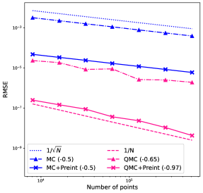
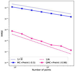
Figure 1: Convergence plots comparing MC and QMC performance (with and without preintegration) for computing the cdf (left) and pdf (right) evaluated at $t=-0.02$ with $\alpha=1$, $\theta=2$ and $16$ random shifts. The numbers in parentheses indicate the empirical rate of convergence.

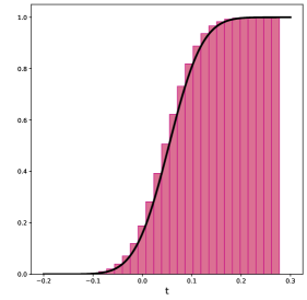
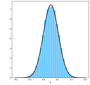
Figure 2: Plots of the computed cdf (left) and pdf (right) for the problem with $\alpha=1$, $\theta=2$ and $N=503$ lattice points. Histograms of 32000 randomly sampled solutions are overlaid.

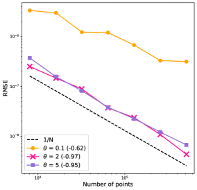
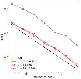
Figure 3: Convergence plots comparing QMC with preintegration performance for computing the cdf at $t=-0.02$ for fixed $\alpha=1$ and varying theta (left) and fixed $\theta=2$ and varying alpha (right) with $16$ random shifts.

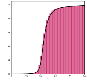
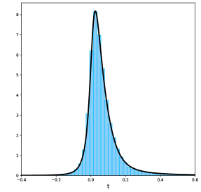
Figure 4: Plots of the cdf (left) and pdf (right) for the problem with $\alpha=30$, $\theta=2$ and $N=503$ lattice points. Histograms of 32000 randomly sampled solutions are overlaid.

The left plot in Figure 3 compares the convergence for the cdf computed using QMC with preintegration for different levels of decay $\theta\in\{0.1,2,5\}$ with $\alpha=1$. For each $\theta$, we construct a new QMC rule using the weights (7.1). We find that the convergence rate is poor for a small decay parameter, whereas for larger decay parameters the convergence rate is close to $\mathcal{O}(N^{-1})$. This is expected since the superposition dimension of the problem decreases as a result of the importance of each parameter decaying faster as $\theta$ increases. The magnitude of the RMSE for $\theta=0.1$ is the largest and for $\theta=2$ and $\theta=5$, the RMSE is comparable.

We are also interested in how the performance of QMC changes as the effect of the random parameters become more dominant. The right plot in Figure 3 compares convergence when $\theta=2$ is fixed and we vary $\alpha\in\{0.1,1,30\}$. We see that the magnitude of the RMSE decreases as the impact of the lognormal random coefficient decreases. The value of $\alpha$ has no obvious impact on the rate of convergence.

Figure 4 shows the cdf and pdf for the case when $\alpha\gg 1$. Here we see the pdf corresponding to $\alpha=30$ is far less symmetrical and is instead positively skewed compared to the density presented in Figure 2 when $\alpha=1$. This is due to the dominance of the lognormal random coefficient in comparison to the Gaussian source term resulting in heavier right tails as one would expect. In Figure 2, where $\alpha=1$, we observe a more symmetrical distribution which looks similar to the Gaussian density. For the case $\alpha\ll 1$ we tested $\alpha=0.1$, in which case the cdf and pdf look very similar to those in Figure 2 and thus have been been omitted.

8 Conclusion

We have presented a new method using preintegration followed by QMC to approximate the cdf and pdf of a quantity of interest from the uncertainty quantification of an elliptic PDE with a lognormally distributed coefficient and a normally distributed source term. The key idea is to formulate the cdf and pdf as an integral of an indicator and Dirac $\delta$ function, respectively. Preintegration is used to smooth the discontinuity in the integrands and then a tailored QMC rule is applied to approximate the remaining integral. We proved that the RMSE of our cdf and pdf approximations converge at a rate close to $1/N$, which is the same rate as for computing the expected value of the quantity of interest. Finally, we presented numerical results showing that the convergence in practice matches the theoretical rates and which demonstrate the superior efficiency of our method compared to plain QMC, as well as MC.

Acknowledgements We would like to extend our appreciation to Ian Sloan for his valuable comments and insights. We also acknowledge the financial support from the Australian Research Council for the project DP210100831.

References

- [1] N. Achtsis, R. Cools, D. Nuyens, Conditional sampling for barrier option pricing under the LT method, SIAM J. Financial Math. 4 (2013), 327–352.
- [2] N. Achtsis, R. Cools, D. Nuyens, Conditional sampling for barrier option pricing under the Heston model, in: J. Dick, F.Y. Kuo, G.W. Peters, I.H. Sloan (eds.), Monte Carlo and Quasi-Monte Carlo Methods (2012), pp. 253–269, Springer-Verlag, Berlin/Heidelberg (2013).
- [3] M. S. Alnaes, J. Blechta, J. Hake, A. Johansson, B. Kehlet, A. Logg, C. Richardson, J. Ring, M. E. Rognes and G. N. Wells. The FEniCS Project Version 1.5, Archive of Numerical Software 3 (2015). doi:doi.org/10.11588/ans.2015.100.20553
- [4] C. Bayer, C. Ben Hammouda, R. Tempone, Numerical smoothing with hierarchical adaptive sparse grids and quasi-Monte Carlo methods for efficient option pricing,
- [5] K. A. Cliffe, I. G. Graham, R. Scheichl, L. Stals, Parallel computation of flow in heterogeneous media using mixed finite elements, J. Comput. Phys. 164 (2000),
- [6] J. Charrier, R. Scheichl, A. L. Teckentrup, Finite element error analysis of elliptic PDEs with random coefficients and its application to multilevel Monte Carlo methods, SIAM J. Numer. Anal. 51 (2013), 322–352.
- [7] P. G. Ciarlet, The Finite Element Method for Elliptic Problems SIAM, Philazdelphia, PA, USA, 2002.
- [8] P. G. Ciarlet, P. A. Raviart, Maximum principle and uniform convergence for the finite element method, Comput. Methods Appl. Mech. Eng. 2 (1973), 17–31.
- [9] K. A. Cliffe, M. B. Giles, R. Scheichl, A. L. Teckentrup, Multilevel Monte Carlo methods and applications to elliptic PDEs with random coefficients, Comput. Visual. Sc. 14 (2011), 3–15.
- [10] J. Dick, F. Y. Kuo, and I. H. Sloan, High dimensional integration — the quasi-Monte Carlo way, Acta Numer. 22 (2013), 133–288.
- [11] D. Dũng, V. K. Nguyen, Ch. Schwab and J. Zech, Analyticity and Sparsity in Uncertainty Quantification for PDEs with Gaussian Random Field Inputs, Springer, Cham (2023).
- [12] L. C. Evans, Partial Differential Equations, American Mathematical Society, Providence, RI, USA, 2010.
- [13] M. Ganesh, F. Y. Kuo, and I. H. Sloan, Quasi-Monte Carlo finite element analysis for wave propagation in heterogeneous random media, SIAM-ASA J. Uncertain. Quantif. 9 (2021), 106–134.
- [14] D. Gilbarg and N. S. Trudinger, Elliptic Partial Differential Equations of Second Order, Springer-Verlag, Berlin-Heidelberg, Germany, 2001.
- [15] A. D. Gilbert, Finite element analysis of density estimation using preintegration for elliptic PDE with random input, in preparation, (2024).
- [16] A. D. Gilbert, I. G. Graham, F. Y. Kuo, R. Scheichl and I. H. Sloan, Analysis of quasi-Monte Carlo methods for elliptic eigenvalue problems with stochastic coefficients, Numer. Math., 142 (2019), 863–915.
- [17] A. D. Gilbert, F. Y. Kuo and I. H. Sloan, Equivalence between Sobolev spaces of first order dominating mixed smoothness and unanchored ANOVA spaces on , Math. Comp., 91 (2022), 1837–1869.
- [18] A. D. Gilbert, F. Y. Kuo and I. H. Sloan, Preintegration is not smoothing when monotonicity fails, in: Z. Botev et al. (eds.) Advances in Modeling and Simulation, Springer, Cham (2022), 169–191.
- [19] A. D. Gilbert, F. Y. Kuo and I. H. Sloan, Analysis of preintegration followed by quasi-Monte Carlo integration for distribution functions and densities, SIAM J. Numer. Anal. 61 (2023),135–166.
- [20] P. Glasserman, Monte Carlo Methods in Financial Engineering, Springer, Berlin (2003).
- [21] P. Glasserman, J. Staum, Conditioning on one-step survival for barrier option simulations, Oper. Res. 49 (2001), 923–937.
- [22] I. G. Graham, F. Y. Kuo, J. A. Nichols, R. Scheichl, Ch. Schwab and I. H. Sloan, Quasi-Monte Carlo finite element methods for elliptic PDEs with lognormal random coefficients, Numer. Math. 131 (2015), 329–368.
- [23] I. G. Graham, F. Y. Kuo, D. Nuyens, R. Scheichl and I. H. Sloan, Quasi-Monte Carlo methods for elliptic PDEs with random coefficients and applications, J. Comput. Phys. 230 (2011), 3668–3694.
- [24] M. Griebel, F. Y. Kuo, and I. H. Sloan, The smoothing effect of the ANOVA decomposition, J. Complexity 26 (2010), 523–551.
- [25] M. Griebel, F. Y. Kuo, and I. H. Sloan, The smoothing effect of integration in and the ANOVA decomposition, Math. Comp. 82 (2013), 383–400.
- [26] M. Griebel, F. Y. Kuo, and I. H. Sloan, Note on “The smoothing effect of integration in and the ANOVA decomposition”, Math. Comp. 86 (2017), 1847–1854.
- [27] M. Griebel, F. Y. Kuo, and I. H. Sloan, The ANOVA decomposition of a non-smooth function of infinitely many variables can have every term smooth, Math. Comp. 86 (2017), 1855– 1876.
- [28] A. Griewank, F. Y. Kuo, H. Leövey, and I. H. Sloan, High dimensional integration of kinks and jumps — smoothing by preintegration, J. Comput. App. Math. 344 (2018), 259–274.
- [29] P. Grisvard, Elliptic Problems in Nonsmooth Domains, SIAM, Philedelphia, USA (2011).
- [30] L. Hermann and Ch. Schwab, QMC integration for lognormal-parametric, elliptic PDEs: local supports and product weights, Numer. Math. 141 (2019), 63–102.
- [31] M. Holtz, Sparse Grid Quadrature in High Dimensions with Applications in Finance and Insurance (PhD thesis), Springer-Verlag, Berlin, 2011.
- [32] J. Indritz, An inequality for Hermite polynomials, Proc. Amer. Math. Soc. 12 (1961), 981–983.
- [33] V. Kaarnioja, F. Y. Kuo, and I. H. Sloan, Lattice-based kernel approximation and serendipitous weights for parametric PDEs in very high dimensions, to appear in: A. Hinrichs, P. Kritzer, F. Pillichshammer (eds.) Monte Carlo and Quasi-Monte Carlo Methods 2022, Springer Verlag.
- [34] J. Karátson, S. Korotov, Discrete maximum principles for finite element solution of nonlinear elliptic problems with mixed boundary conditions, Numer. Math. 99 (2005), 669–698.
- [35] Y. Kazashi, Quasi-Monte Carlo integration with product weights for elliptic PDEs with log-normal coefficients, IMA J. Numer. Anal. 39 (2019), 1563–1593.
- [36] F. Y. Kuo, C. Schwab, I. H. Sloan, Quasi-Monte Carlo finite element methods for a class of elliptic partial differential equations with random coefficients, SIAM J. Numer. Anal. 50 (2012), 3351–3374.
- [37] F. Y. Kuo, I. H. Sloan, G. W. Wasilkowski and B. J. Waterhouse, Randomly shifted lattice rules with the optimal rate of convergence for unbounded integrands, J. Complexity 26 (2010), 135–160.
- [38] J. A. Nichols and F. Y. Kuo, Fast CBC construction of randomly shifted lattice rules achieving convergence for unbounded integrands over in weighted spaces with POD weights, J. Complexity 30 (2014), 444–468.
- [39] A. Logg, K. A. Mardal, G. N. Wells et al., Automated Solution of Differential Equations by the Finite Element Method, Springer (2012). doi: 10.1007/978-3-642-23099-8
- [40] A. Logg and G. N. Wells, DOLFIN: Automated Finite Element Computing, ACM Transactions on Mathematical Software 37 (2010). doi: 10.1145/1731022.1731030
- [41] A. Logg, G. N. Wells and J. Hake, DOLFIN: a C++/Python Finite Element Library, in: A. Logg, K. A. Mardal and G. N. Wells (eds) Automated Solution of Differential Equations by the Finite Element Method (chapter 10), volume 84 of Lecture Notes in Computational Science and Engineering, Springer (2012)
- [42] P. L’Ecuyer, C. Lemieux, Variance reduction via lattice rules, Manag. Sci. 46 (2000), 1214–1235.
- [43] P. L’Ecuyer, F. Puchhammer, A. Ben Abdellah, Monte Carlo and quasi-Monte Carlo density estimation via conditioning, INFORMS J. Comput. 34, (2022), 1729–1748.
- [44] S. Liu, A. B. Owen, Preintegration via active subspaces, SIAM J. Numer. Anal. 61 (2023), 495–514.
- [45] PVC (Research Infrastructure), UNSW Sydney, Katana. (2010) doi: 10.26190/669X-A286
- [46] A. L. Teckentrup, R. Scheichl, M. B. Giles, and E. Ullmann, Further analysis of multilevel Monte Carlo methods for elliptic PDEs with random coefficients, Numer. Math. 125 (2013), 569–600.
- [47] C. Weng, X. Wang, Z. He, Efficient computation of option prices and greeks by quasi-Monte Carlo method with smoothing and dimension reduction, SIAM J. Sci. Comput. 39 (2017), B298–B322.