Theory of the spectral function of Fermi polarons at finite temperature

Abstract

We develop a general theory of Fermi polarons at nonzero temperature, including particle-hole excitations of the Fermi sea shake-up to arbitrarily high orders. The exact set of equations of the spectral function is derived by using both Chevy ansatz and diagrammatic approach, and their equivalence is clarified to hold in free space only, with an unregularized infinitesimal interaction strength. The correction to the polaron spectral function arising from two-particle-hole excitations is explicitly examined, for an exemplary case of Fermi polarons in one-dimensional optical lattices. We find quantitative improvements at low temperatures with the inclusion of two-particle-hole excitations, in both polaron energies and decay rates. Our exact theory of Fermi polarons with arbitrary orders of particle-hole excitations might be used to better understand the intriguing polaron dynamical responses in two or three dimensions, whether in free space or within lattices.

Fermi polarons, which are quasiparticles describing the collective motion of an impurity as it interacts with and shakes up a Fermi sea, manifest in various realms of condensed matter physics (Alexandrov2010, ). This well-established concept underlies a number of fantastic quantum many-body phenomena, including Anderson orthogonality catastrophe (Anderson1967, ), the Fermi edge singularity in x-ray spectra (Mahan1967, ; Nozieres1969, ), and Nagaoka ferromagnetism (Nagaoka1966, ; Shastry1990, ; Cui2010, ). The recent realization of atomic Fermi gases with spin-population imbalance opens a new paradigm to quantitatively explore Fermi polaron physics in untouched territory (Massignan2014, ; Schmidt2018, ), owing to the unprecedented controllability of ultracold atoms (Bloch2008, ), particularly in interatomic interactions (Chin2010, ). Thus far, considerable attention has been given to investigating the ground state of Fermi polarons (Massignan2014, ), known as attractive polarons, through both experimental and theoretical means. The attractive polaron energy has been calculated to great accuracy, by using methods such as variational Chevy ansatz (Chevy2006, ; Combescot2008, ; Giraud2010, ), diagrammatic $T$-matrix approach (Giraud2010, ; Combescot2007, ; Hu2018, ; Mulkerin2019, ; Tajima2019, ; Hu2022, ), functional renormalization group (Schmidt2011, ; vonMilczewski2024, ), and quantum Monte Carlo simulations (Prokofev2008, ). The outcomes of these predictions align remarkably well with spectroscopic measurements, including radio-frequency (rf) spectroscopy (Schirotzek2009, ; Zhang2012, ; Zan2019, ), Ramsey interferometry (Cetina2016, ), Rabi cycle (Scazza2017, ; Vivanco2024, ), and Raman spectroscopy (Ness2020, ).

In contrast, describing the excited states of Fermi polarons proves to be notably challenging (Goulko2016, ), especially when departing from the heavy impurity limit, where exact numerical calculations might be feasible (Schmidt2018, ; Knap2012, ; Wang2022PRL, ; Wang2022PRA, ). As a result, the finite-temperature dynamical responses of Fermi polarons related to excited states, as assessed by various spectroscopic studies, are less well understood. Specifically, in the case of unitary Fermi polarons with an infinitely large scattering length at degenerate temperature, state-of-the-art diagrammatic $T$-matrix theory (Tajima2019, ; Hu2022, ) falls short in explaining the spectral features observed in the rf spectroscopy (Zan2019, ). These features unveil the abrupt dissolution of the attractive polaron, leading to the emergence of excited branches featuring either repulsive polarons or dressed dimerons. Additionally, the theory struggles to provide a quantitative explanation for the observed Raman spectra (Hu2022Raman, ), when the interaction between the impurity and Fermi sea becomes strong. The inadequacy of the theory at nonzero temperature may stem from its insufficient description of the Fermi sea shake-up, as it only includes one-particle-hole excitations of the Fermi sea (Combescot2007, ; Hu2022, ).

In this Letter, we present a formally exact finite-temperature theory of Fermi polarons, incorporating arbitrary numbers of particle-hole excitations of the Fermi sea. We use two methods to derive an exact set of equations for the fundamental quantity of the polaron spectral function, which determines the rf, Ramsey and Raman spectroscopies. The first method of Chevy ansatz is generally applicable to any interaction potential, while the second diagrammatic approach is restricted to a contact interaction in free space, whose unregularized strength is infinitesimal. We establish the equivalence of the two approaches when they are both valid and show that the coefficients in Chevy ansatz can be directly expressed in terms of the many-particle vertex functions in the diagrammatic theory. A more comprehensive discussion of the derivation and comparison of these two approaches is presented in a companion paper (LongPRA2024, ).

The exact set of equation for the spectral function can be truncated to enclose, to a particular order (i.e., $n$-th order with $n$ particle-hole excitations). To illustrate, we focus on Fermi polarons in one-dimensional lattices and analyze the enhanced predictive capabilities of the spectral function when two-particle-hole excitations are taken into account. Future studies with more involved numerical efforts would be beneficial in providing quantitative predictions for the finite-temperature spectral function of unitary Fermi polarons in three-dimensional free space, and would offer insights into elucidating the perplexing spectral features observed in rf and Raman spectroscopies thus far (Zan2019, ; Ness2020, ).

Chevy ansatz at finite T. Following the seminal works by Chevy (Chevy2006, ) and Combescot and Giraud (Combescot2008, ), we take the following Chevy ansatz for a single spin-down atom (i.e., impurity) immersed in a Fermi sea of spin-up atoms with a total momentum $\mathbf{p}$,

$$\left|\psi\right\rangle=\sum_{n=0}^{\infty}\left|\psi_{n}\right\rangle=\sum_{n=0}^{\infty}\frac{1}{\left(n!\right)^{2}}\sum_{\{\mathbf{k}\mathbf{q}\}}\alpha_{\mathbf{q}_{1}\mathbf{q}_{2}\cdots\mathbf{q}_{n}}^{\mathbf{k}_{1}\mathbf{k}_{2}\cdots\mathbf{k}_{n}}d_{\mathbf{p}-\mathbf{P}_{\vec{\kappa}_{n}}}^{\dagger}\left|\vec{\kappa}_{n}\right\rangle,$$ (1)

where $d_{\mathbf{p}}^{\dagger}$ and $c_{\mathbf{k}}^{\dagger}$ are respectively the creation field operators of the impurity and spin-up atoms, and $\left|\vec{\kappa}_{n}\right\rangle\equiv c_{\mathbf{k}_{1}}^{\dagger}\cdots c_{\mathbf{k}_{n}}^{\dagger}c_{\mathbf{q}_{n}}\cdots c_{\mathbf{q}_{1}}\left|\textrm{FS}\right\rangle$ describes $n$-particle-hole excitations out of a thermal Fermi sea $\left|\textrm{FS}\right\rangle$, with a momentum $\mathbf{P}_{\vec{\kappa}_{n}}=(\mathbf{k}_{1}+\cdots+\mathbf{k}_{n})-(\mathbf{q}_{1}+\cdots+\mathbf{q}_{n})$. The occupation of each state $\mathbf{k}$ in the thermal Fermi sea is given by the Fermi distribution function $f(\xi_{\mathbf{k}})=1/(e^{\xi_{\mathbf{k}}/k_{B}T}+1)$, where $\xi_{\mathbf{k}}=\varepsilon_{\mathbf{k}}-\mu$ is the dispersion of spin-up atoms, measured from the chemical potential $\mu$. Due to the anti-commutation of fermionic field operators, the coefficients $\alpha_{\mathbf{q}_{1}\mathbf{q}_{2}\cdots\mathbf{q}_{n}}^{\mathbf{k}_{1}\mathbf{k}_{2}\cdots\mathbf{k}_{n}}$ are antisymmetric upon exchanging $\mathbf{k}_{i}$ and $\mathbf{k}_{j}$ or $\mathbf{q}_{i}$ and $\mathbf{q}_{j}$, where $i,j=1,\cdots,n$. The resulting redundancy is removed by the factor $1/(n!)^{2}$.

We solve the Schrödinger equation, $\mathcal{H}\left|\psi\right\rangle=(\mathcal{H}_{0}+\mathcal{H}_{\textrm{int}})\left|\psi\right\rangle=E\left|\psi\right\rangle$, based on a crucial observation that $\mathcal{H}\left|\psi_{n}\right\rangle$ can be conveniently expressed by a combination of the terms $d_{\mathbf{p}-\mathbf{P}_{\vec{\kappa}_{m}}}^{\dagger}\left|\vec{\kappa}_{m}\right\rangle$, where $m=n-1$, $n$, and $n+1$, so we may directly write down a set of equations for the coefficients. The action of the non-interacting, kinetic part of the Hamiltonian on the wavefunction is easy to work out (LongPRA2024, ), $\mathcal{H}_{0}\left|\psi_{n}\right\rangle=1/(n!)^{2}\sum_{\{\mathbf{k}\mathbf{q}\}}(E_{\textrm{FS}}+\varepsilon_{\mathbf{p}-\mathbf{P}_{\vec{\kappa}_{n}}}^{I}+E_{\vec{\kappa}_{n}})\alpha_{\mathbf{q}_{1}\mathbf{q}_{2}\cdots\mathbf{q}_{n}}^{\mathbf{k}_{1}\mathbf{k}_{2}\cdots\mathbf{k}_{n}}d_{\mathbf{p}-\mathbf{P}_{\vec{\kappa}_{n}}}^{\dagger}\left|\vec{\kappa}_{n}\right\rangle$, where $E_{\textrm{FS}}$ is the energy of the thermal Fermi sea, $E_{\vec{\kappa}_{n}}=(\varepsilon_{\mathbf{k}_{1}}+\cdots+\varepsilon_{\mathbf{k}_{n}})-(\varepsilon_{\mathbf{q}_{1}}+\cdots+\varepsilon_{\mathbf{q}_{n}})$ is the excitation energy of $n$ particles and holes, and $\varepsilon_{\mathbf{p}}^{I}$ is the impurity dispersion relation. The action of the interaction Hamiltonian on $\left|\psi_{n}\right\rangle$ is also straightforward to obtain, after some tedious algebra (LongPRA2024, ). For the simple case of a contact interaction (in free space) or an on-site interaction (in lattices) with strength $U$, we find

$$-E_{\mathbf{p};\{\mathbf{k}\};\{\mathbf{q}\}}^{(n)}\alpha_{\mathbf{q}_{1}\mathbf{q}_{2}\cdots\mathbf{q}_{n}}^{\mathbf{k}_{1}\mathbf{k}_{2}\cdots\mathbf{k}_{n}} = U\sum_{i,j=1,\cdots,n}\left(-1\right)^{i+j}\alpha_{\mathbf{q}_{1}\cdots\mathbf{q}_{n-j}\mathbf{q}_{n-j+2}\cdots\mathbf{q}_{n}}^{\mathbf{k}_{1}\cdots\mathbf{k}_{n-i}\mathbf{k}_{n-i+2}\cdots\mathbf{k}_{n}}+U\left[\sum_{\mathbf{K}}\left(\alpha_{\mathbf{q}_{1}\mathbf{q}_{2}\cdots\mathbf{q}_{n}}^{\mathbf{K}\mathbf{k}_{2}\cdots\mathbf{k}_{n}}+\cdots+\alpha_{\mathbf{q}_{1}\mathbf{q}_{2}\cdots\mathbf{q}_{n}}^{\mathbf{k}_{1}\cdots\mathbf{k}_{n-1}\mathbf{K}}\right)f\left(-\xi_{\mathbf{K}}\right)\right.$$ (2)

$$\left.-\sum_{\mathbf{Q}}\left(\alpha_{\mathbf{Q}\mathbf{q}_{2}\cdots\mathbf{q}_{n}}^{\mathbf{k}_{1}\mathbf{k}_{2}\cdots\mathbf{k}_{n}}+\cdots+\alpha_{\mathbf{q}_{1}\cdots\mathbf{q}_{n-1}\mathbf{Q}}^{\mathbf{k}_{1}\mathbf{k}_{2}\cdots\mathbf{k}_{n}}\right)f\left(\xi_{\mathbf{Q}}\right)\right]+U\sum_{\mathbf{KQ}}\alpha_{\mathbf{q}_{1}\mathbf{q}_{2}\cdots\mathbf{q}_{n}\mathbf{Q}}^{\mathbf{k}_{1}\mathbf{k}_{2}\cdots\mathbf{k}_{n}\mathbf{K}}f\left(-\xi_{\mathbf{K}}\right)f\left(\xi_{\mathbf{Q}}\right),$$

where $E_{\mathbf{p};\{\mathbf{k}\};\{\mathbf{q}\}}^{(n)}\equiv-(E-E_{\textrm{FS}}-\nu U)+\varepsilon_{\mathbf{p}-\mathbf{P}_{\vec{\kappa}_{n}}}^{I}+E_{\vec{\kappa}_{n}}$ at the density (or filling factor) $\nu$, and the left-hand-side of the equation shows the coefficient of $(E-\mathcal{H}_{0}-\nu U)\left|\psi_{n}\right\rangle$. The three terms on the right-hand-side of the equation come from $(\mathcal{H}_{\textrm{int}}-\nu U)\left|\psi\right\rangle$, involving a summation over the particle momentum $\mathbf{K}$ or the hole momentum $\mathbf{Q}$, which carries either a distribution function $f(-\xi_{\mathbf{K}})=1-f(\xi_{\mathbf{K}})$ or $f(\xi_{\mathbf{Q}})$. It is easy to see, Eq. (2) has a nice hierarchy structure. In particular, once we discard the last term on the right-hand-side at a given order, the set of equations for the coefficients $\alpha_{\mathbf{q}_{1}\mathbf{q}_{2}\cdots\mathbf{q}_{n}}^{\mathbf{k}_{1}\mathbf{k}_{2}\cdots\mathbf{k}_{n}}$ encloses.

At zero temperature, where the sharp Fermi surface at the Fermi wavevector $k_{F}$ separates the momenta $\left|\mathbf{k}_{i}\right|>k_{F}$ and $\left|\mathbf{q}_{i}\right|<k_{F}$, Eq. (2) was already derived, up to the second order $n=2$ (Combescot2008, ) and $n=3$ (Liu2022, ). At nonzero temperature, the first-order truncation of Eq. (2) was also recently discussed (Liu2019, ). All these studies emphasize that Chevy ansatz is variational, so their focus is more on some individual many-body eigenstates of the system. Here, we are interested in attractive or repulsive polarons, which may consist of a bundle of many-body eigenstates. The polaron energy at nonzero temperature does not necessarily become smaller as we increase the order of particle-hole excitations. It is therefore more useful to describe Fermi polarons using the polaron Green function. For this purpose, we may take a continuous variable $\omega\equiv E-E_{\textrm{FS}}-\nu U$ and interpret Eq. (2) at the leading order, i.e., $(\omega-\varepsilon_{\mathbf{p}}^{I})\alpha_{0}=U\sum_{\mathbf{KQ}}\alpha_{\mathbf{Q}}^{\mathbf{K}}f\left(-\xi_{\mathbf{K}}\right)f\left(\xi_{\mathbf{Q}}\right)$, as the condition for the poles of the polaron Green function. Indeed, we are free to take an un-normalized ansatz with $\alpha_{0}=1$ and consequently identify the polaron self-energy,

$$\Sigma\left(\mathbf{p},\omega\right)=U\sum_{\mathbf{KQ}}\alpha_{\mathbf{Q}}^{\mathbf{K}}f\left(-\xi_{\mathbf{K}}\right)f\left(\xi_{\mathbf{Q}}\right).$$ (3)

We will soon rigorously examine this identification by using the diagrammatic theory. Thus, for a given $\mathbf{p}$ and $\omega$, if we are able to solve the set of Eq. (2) truncated to a particular order $n$, we may directly calculate the polaron Green function $G_{\downarrow}(\mathbf{p},\omega)$ and hence the spectral function $A(\mathbf{p},\omega)=-\textrm{Im$G_{\downarrow}$($\mathbf{p}$,$\omega$)}/\pi$, with the inclusion of $n$ particle-hole excitations of the Fermi sea.

Chevy ansatz with $U=0^{-}$. In free space and in two or three dimensions, the contact interaction should be regularized by using an $s$-wave scattering length. Formally, the interaction strength $U$ becomes infinitesimal, in order to remove the ultraviolet divergence at large momentum. In this situation, in Eq. (2) the terms involving a summation over $\mathbf{Q}$ vanish and we may simplify the equation, by defining the variables, $G_{\mathbf{q}_{1}\mathbf{q}_{2}\cdots\mathbf{q}_{n}}^{\mathbf{k}_{1}\mathbf{k}_{2}\cdots\mathbf{k}_{n-1}}\equiv U\sum_{\mathbf{K}}\alpha_{\mathbf{q}_{1}\mathbf{q}_{2}\cdots\mathbf{q}_{n}}^{\mathbf{k}_{1}\cdots\mathbf{k}_{n-1}\mathbf{K}}f\left(-\xi_{\mathbf{K}}\right)$. It is then straightforward to derive the following set of equations (LongPRA2024, ),

$$G_{\mathbf{q}_{1}\mathbf{q}_{2}\cdots\mathbf{q}_{n}}^{\mathbf{k}_{1}\mathbf{k}_{2}\cdots\mathbf{k}_{n-1}} = \left[\frac{1}{U}+\sum_{\mathbf{K}}\frac{f\left(-\xi_{\mathbf{K}}\right)}{E_{\mathbf{p};\mathbf{k}_{1}\mathbf{k}_{2}\cdots\mathbf{K};\mathbf{q}_{1}\mathbf{q}_{2}\cdots\mathbf{q}_{n}}^{(n)}}\right]^{-1}\left[\sum_{j=1}^{n}(-1)^{j-1}\alpha_{\mathbf{q}_{1}\mathbf{q}_{2}\cdots\mathbf{q}_{n-j}\mathbf{q}_{n-j+2}\cdots\mathbf{q}_{n}}^{\mathbf{k}_{1}\mathbf{k}_{2}\cdots\mathbf{k}_{n-1}}+\right.$$ (4)

$$\left.\sum_{\mathbf{K}}\frac{\sum_{i=1}^{n-1}G_{\mathbf{q}_{1}\mathbf{q}_{2}\cdots\mathbf{q}_{n}}^{\mathbf{k}_{1}\mathbf{k}_{2}\cdots\mathbf{k}_{n-i-1}\mathbf{K}\mathbf{k}_{n-i+1}\cdots\mathbf{k}_{n-1}}}{E_{\mathbf{p};\mathbf{k}_{1}\mathbf{k}_{2}\cdots\mathbf{K};\mathbf{q}_{1}\mathbf{q}_{2}\cdots\mathbf{q}_{n}}^{(n)}}f\left(-\xi_{\mathbf{K}}\right)-\sum_{\mathbf{K}\mathbf{Q}}\frac{G_{\mathbf{q}_{1}\mathbf{q}_{2}\cdots\mathbf{q}_{n}\mathbf{Q}}^{\mathbf{k}_{1}\mathbf{k}_{2}\cdots\mathbf{k}_{n-1}\mathbf{K}}}{E_{\mathbf{p};\mathbf{k}_{1}\mathbf{k}_{2}\cdots\mathbf{K};\mathbf{q}_{1}\mathbf{q}_{2}\cdots\mathbf{q}_{n}}^{(n)}}f\left(-\xi_{\mathbf{K}}\right)f\left(\xi_{\mathbf{Q}}\right)\right],$$

which are manifestly antisymmetric with respect to the exchange of two momenta in $\mathbf{k}_{i}$ or $\mathbf{q}_{i}$. As we shall see, these seemingly complicated equations have an elegant explanation in terms of Feynman diagrams.

Diagrammatic theory. To this aim, let us introduce the ($n+1$)-particle vertex function $\Gamma_{n+1}(\{k_{l}\};p,\{q{}_{l}\})$, which describes the in-medium scatterings among $n$ spin-up atoms in the Fermi sea and the impurity. The collective notation $\{k_{l}\}$ stands for $k_{1}k_{2}\cdots k_{n}$, where the incoming four-momentum $k_{l}\equiv(\mathbf{k}_{l},i\omega_{l})$ and $\omega_{l}\equiv(2m_{l}+1)\pi k_{B}T$ is the fermionic Matsubara frequency with integer $m_{l}$. The same notation is similarly taken for the out-going momenta {$q_{l}$}. We require the spin-up atom with the incoming four-momentum $k_{n}$ interacts first with the impurity. While it is not so obvious at this point, the vertex function $\Gamma_{n+1}$ does not depend on $k_{n}$ when $n\geq 2$ (LongPRA2024, ). As such, $\Gamma_{n+1}$ is antisymmetric when we exchange any two momenta in $\{k_{l}\}_{l\neq n}$ or $\{q_{l}\}$.

Figure 1: Polaron self-energy $\Sigma(p)$ expressed in terms of the vertex function $\Gamma_{2}(k;p,q)$ (see the upper panel), whose diagrammatic contributions are explicitly listed in the lower panel, with building blocks of the $T$-matrix $T_{2}(p+q)$ and the three-body vertex function $\Gamma_{3}(kk^{\prime};p,qq^{\prime})$.

We find that the coefficients in the Chevy ansatz are related to the many-particle vertex functions $\Gamma_{n+1}$ (LongPRA2024, ),

$$\alpha_{\mathbf{q}_{1}\mathbf{q}_{2}\cdots\mathbf{q}_{n}}^{\mathbf{k}_{1}\mathbf{k}_{2}\cdots\mathbf{k}_{n}}=-\frac{\Gamma_{n+1}\left(\{k_{l}\}_{l\neq n};p,\{q_{l}\}\right)}{E_{\mathbf{p};\{\mathbf{k}\};\{\mathbf{q}\}}^{(n)}},$$ (5)

where all the four momenta take the on-shell values, such as $p\equiv(\mathbf{p},\omega)$, $k_{i}\equiv(\mathbf{k}_{i},\xi_{\mathbf{k}_{i}})$ and $q_{i}=(\mathbf{q}_{i},\xi_{\mathbf{q}_{i}})$. By integrating over $\mathbf{k}_{n}$ on both sides of the equation and recalling the fact that $\Gamma_{n+1}$ does not depend on $\mathbf{k}_{n}$, we obtain $G_{\mathbf{q}_{1}\mathbf{q}_{2}\cdots\mathbf{q}_{n}}^{\mathbf{k}_{1}\mathbf{k}_{2}\cdots\mathbf{k}_{n-1}}=\Gamma_{n+1}\left(\{k_{l}\}_{l\neq n};p,\{q{}_{l}\}\right)$ for $n\geq 2$.

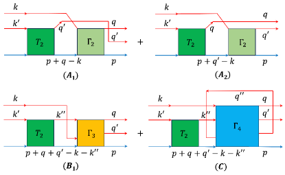
Figure 2: Diagrammatic contributions to the three-body vertex function $\Gamma_{3}(kk^{\prime};p,qq^{\prime})$, classified into three different types of diagrams, $A$, $B$ and $C$, which correspond to the three terms on the right-hand-side of Eq. (4).

The relations Eq. (3) and Eq. (5) are the key results of our Letter, as they clearly demonstrate the powerfulness of Chevy ansatz in the case of just a few impurities, which may provide useful insights into further developing accurate diagrammatic theories for strong correlated systems. To establish the relations, let us first examine the Dyson equation, which is diagrammatically shown in Fig. 1. There, as the impurity line can only propagate forward (Mahan1967, ; Nozieres1969, ), the vertex function $\Gamma_{2}$ can be fully represented by three diagrams, where $T_{2}$ is the standard $T$-matrix that sums up the infinite ladder diagrams. Similarly, the three-particle vertex function $\Gamma_{3}$ is completely represented by four diagrams as given in Fig. 2. In the companion paper (LongPRA2024, ), we also provide the diagrammatic contributions to the four-particle vertex function $\Gamma_{4}$.

From Fig. 2, it is not difficult to write down the on-shell expression of $\Gamma_{3}$, after we sum over two internal Matsubara frequencies (LongPRA2024, ),

$$\frac{\Gamma_{3}\left(k;p,qq^{\prime}\right)}{T_{2}\left(p+q+q^{\prime}-k\right)}=A_{1}+A_{2}+B_{1}+C,$$ (6)

where $T_{2}^{-1}(p+q+q^{\prime}-k)=1/U+\sum_{\mathbf{k}^{\prime}}f(-\xi_{\mathbf{k}^{\prime}})/E_{\mathbf{p};\mathbf{kk}^{\prime};\mathbf{qq}^{\prime}}^{(2)}$ is the inverse $T$-matrix, and $A_{1}=-\Gamma_{2}(k;p,q)/E_{\mathbf{p};\mathbf{k};\mathbf{q}}^{(1)}=\alpha_{\mathbf{q}}^{\mathbf{k}}$ and $A_{2}=\Gamma_{2}(k;p,q^{\prime})/E_{\mathbf{p};\mathbf{k};\mathbf{q}^{\prime}}^{(1)}=-\alpha_{\mathbf{q^{\prime}}}^{\mathbf{k}}$ are the contributions from the diagrams ($A_{1}$) and ($A_{2}$), respectively. Finally, the remaining two diagrams give rise to $B_{1}=\sum_{\mathbf{k}^{\prime}}f(-\xi_{\mathbf{k}^{\prime}})\Gamma_{3}(k^{\prime};p,qq^{\prime})/E_{\mathbf{p};\mathbf{kk}^{\prime};\mathbf{qq}^{\prime}}^{(2)}$ and $C=-\sum_{\mathbf{k}^{\prime}\mathbf{q^{\prime\prime}}}f(-\xi_{\mathbf{k}^{\prime}})f(\xi_{\mathbf{q^{\prime\prime}}})\Gamma_{4}(kk^{\prime};p,qq^{\prime}q^{\prime\prime})/E_{\mathbf{p};\mathbf{kk}^{\prime};\mathbf{qq}^{\prime}}^{(2)}$. It is easy to check that, in Eq. (6) by further replacing $\Gamma_{3}(k^{\prime};p,qq^{\prime})$ by $G_{\mathbf{qq}^{\prime}}^{\mathbf{k}}$ and $\Gamma_{4}(kk^{\prime};p,qq^{\prime}q^{\prime\prime})$ by $G_{\mathbf{qq}^{\prime}\mathbf{q}^{\prime\prime}}^{\mathbf{kk}^{\prime}}$, we indeed recover Eq. (4) at the second order $n=2$. Quite generally, the diagrams of the many-particle vertex function $\Gamma_{n+1}$ can be categorized into types $A$, $B$ and $C$, which exactly correspond to the three terms on the right-hand-side of Eq. (4), respectively (LongPRA2024, ). The on-shell expression of $\Gamma_{2}$ can be similarly determined using Fig. 1. In particular, the Dyson equation reads (LongPRA2024, ), $\Sigma(\mathbf{p},\omega)=-U\sum_{\mathbf{kq}}f(-\xi_{\mathbf{k}})f(\xi_{\mathbf{q}})\Gamma_{2}(k;p,q)/E_{\mathbf{p};\mathbf{k};\mathbf{q}}^{(1)}$, which is precisely Eq. (3), once we use the relation Eq. (5) to replace $-\Gamma_{2}/E_{\mathbf{p};\mathbf{k};\mathbf{q}}^{(1)}$ with $\alpha_{\mathbf{q}}^{\mathbf{k}}$.

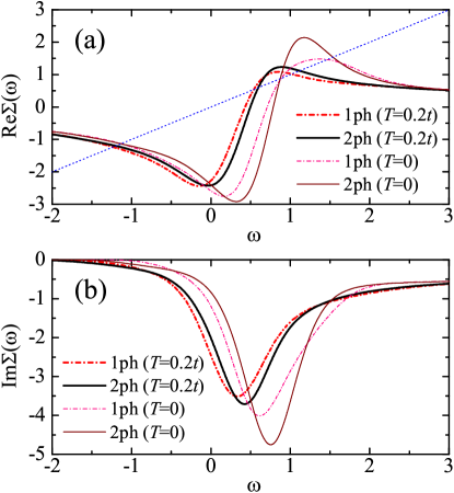
Figure 3: The real part (a) and imaginary part (b) of the polaron self-energy $\Sigma(\mathbf{p}=0,\omega)$ at zero momentum. The solid lines and dash-dotted lines correspond to the results with and without two-particle-hole (2ph) excitations, respectively. The blue dotted line in (a) shows $\omega-E_{\mathbf{p}=0}$ and its crossing points with $\textrm{Re}\Sigma$ give rise to the polaron energies. Here, we take the filling factor $\nu=0.2$, the on-site interaction strength $U=-4t$, and an impurity hopping amplitude $t_{d}=t$. Both the self-energy $\Sigma$ and the frequency $\omega$ are measured in units of the hopping amplitude of atoms $t$.

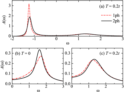
Figure 4: (a) The zero-momentum polaron spectral function $A(\mathbf{p}=0,\omega)$ at the temperature $T=0.2t$. (b) and (c) highlight the repulsive polaron responses at $\omega\sim 1.5t$, at zero temperature $T=0$ and at $T=0.2t$, respectively. The black solid lines or red dash-dotted lines show the predictions with or without two-particle-hole excitations. The other parameters are the same as in Fig. 3.

Fermi polarons in lattices. The exact sets of Eq. (2) and Eq. (4) could be implemented to calculate the polaron self-energy in Eq. (3) and hence the polaron spectral function. However, numerical calculations at finite temperature are challenging, due to the zeros of $E_{\mathbf{p};\{\mathbf{k}\}\{\mathbf{q}\}}^{(n)}$ that make the coefficients $\alpha_{\mathbf{q}_{1}\mathbf{q}_{2}\cdots\mathbf{q}_{n}}^{\mathbf{k}_{1}\mathbf{k}_{2}\cdots\mathbf{k}_{n}}$ and $G_{\mathbf{q}_{1}\mathbf{q}_{2}\cdots\mathbf{q}_{n}}^{\mathbf{k}_{1}\mathbf{k}_{2}\cdots\mathbf{k}_{n-1}}$ highly singular. As a result, the truncation to one-particle-hole excitations was only recently considered (Mulkerin2019, ; Tajima2019, ; Hu2022, ; Liu2019, ). Further improvements to the level of two-particle-hole excitations have never been attempted.

Here, we focus on Fermi polarons in one-dimensional lattices with an on-site attraction $U<0$, a situation that can be readily realized in cold-atom experiments. We solve Eq. (2) with the inclusion of two-particle-hole excitations (LongPRA2024, ). The singularities in the coefficients are removed by introducing a finite broadening factor $\eta$ to the frequency, i.e., $\omega\rightarrow\omega_{\eta}\equiv\omega+i\eta$. We take several broadening factors at the order of the hopping amplitude of atoms $t$, and eventually extrapolate to the zero broadening limit, $\eta=0^{+}$.

In Fig. 3, we report the polaron self-energy at zero temperature and at $T=0.2t$, calculated with one-particle-hole excitations only (red dot-dashed lines) and with two-particle-hole excitations (black solid lines). We find quantitative improvements when we incorporate two-particle-hole excitations at both temperatures. However, the improvement becomes less significant with increasing temperature. In Fig. 4(a), we present the polaron spectral function at $T=0.2t$, which clearly shows the attractive branch (at $\omega\sim-1.3t$) and repulsive branch (at $\omega\sim 1.5t$). The inclusion of two-particle-hole excitations leads to a larger decay rate for the attractive polaron and thereby a reduced attractive polaron peak. It also slightly increases attractive polaron energy. In contrast, for the repulsive polaron, two-particle-hole excitations enhance the peak height, as revealed by Fig. 4(c). This enhancement is particularly evident at zero temperature, as shown in Fig. 4(b).

Conclusions. In summary, we have derived an exact set of equations, to determine the spectral function of Fermi polarons, by using both Chevy ansatz and the diagrammatic approach. Our exact theory incorporates arbitrary numbers of particle-hole excitations, allowing a systematic check of the importance of particle-hole excitations at different level. We have calculated the spectral function of Fermi polarons in one-dimensional lattices and have examined the improvement due to the inclusion of two-particle-hole excitations. The extension of our calculations to a unitary Fermi polaron, with more elaborate numerical efforts, might be used to quantitatively understand the puzzling spectral feature observed in recent measurements (Zan2019, ; Ness2020, ). Furthermore, our exact formalism is also directly applicable to investigate the few-body (i.e., $n+1$) bound states, which emerge as the poles of the many-particle vertex functions $\Gamma_{n+1}$ , both in vacuum or in the presence of the Fermi sea.

- (1) A. S. Alexandrov and J. T. Devreese, Advances in Polaron Physics (Springer, New York, 2010), Vol. 159.
- (2) P. W. Anderson, Infrared Catastrophe in Fermi Gases with Local Scattering Potentials, Phys. Rev. Lett. 18, 1049 (1967).
- (3) G. D. Mahan, Excitons in Metals: Infinite Hole Mass, Phys. Rev. 163, 612 (1967).
- (4) P. Nozières and C. T. De Dominicis, Singularities in the X-Ray Absorption and Emission of Metals. III. One- Body Theory Exact Solution, Phys. Rev. 178, 1097 (1969).
- (5) Y. Nagaoka, Ferromagnetism in a Narrow, Almost Half-Filled Band, Phys. Rev. 147, 392 (1966).
- (6) B. S. Shastry, H. R. Krishnamurthy, and P. W. Anderson, Instability of the Nagaoka ferromagnetic state of the Hubbard model, Phys. Rev. B 41, 2375 (1990).
- (7) X. Cui and H. Zhai, Stability of a fully magnetized ferromagnetic state in repulsively interacting ultracold Fermi gases, Phys. Rev. A 81, 041602(R) (2010).
- (8) P. Massignan, M. Zaccanti, and G. M. Bruun, Polarons, dressed molecules and itinerant ferromagnetism in ultracold Fermi gases, Rep. Prog. Phys. 77, 034401 (2014).
- (9) R. Schmidt, M. Knap, D. A. Ivanov, J.-S. You, M. Cetina, and E. Demler, Universal many-body response of heavy impurities coupled to a Fermi sea: a review of recent progress, Rep. Prog. Phys. 81, 024401 (2018).
- (10) I. Bloch, J. Dalibard, and W. Zwerger, Many-body physics with ultracold gases, Rev. Mod. Phys. 80, 885 (2008).
- (11) C. Chin, R. Grimm, P. Julienne, and E. Tiesinga, Feshbach resonances in ultracold gases, Rev. Mod. Phys. 82, 1225 (2010).
- (12) F. Chevy, Universal phase diagram of a strongly interacting Fermi gas with unbalanced spin populations, Phys. Rev. A 74, 063628 (2006).
- (13) R. Combescot and S. Giraud, Normal State of Highly Polarized Fermi Gases: Full Many-Body Treatment, Phys. Rev. Lett. 101, 050404 (2008).
- (14) S. Giraud, Contribution à la théorie des gaz de fermions ultrafroids fortement polarisés (PhD Thesis 2010).
- (15) R. Combescot, A. Recati, C. Lobo, and F. Chevy, Normal State of Highly Polarized Fermi Gases: Simple Many-Body Approaches, Phys. Rev. Lett. 98, 180402 (2007).
- (16) H. Hu, B. C. Mulkerin, J. Wang, and X.-J. Liu, Attractive Fermi polarons at nonzero temperatures with a finite impurity concentration, Phys. Rev. A 98, 013626 (2018).
- (17) B. C. Mulkerin, X.-J. Liu, and Hui Hu, Breakdown of the Fermi polaron description near Fermi degeneracy at unitarity, Ann. Phys. (N. Y.) 407, 29 (2019).
- (18) H. Tajima and S. Uchino, Thermal crossover, transition, and coexistence in Fermi polaronic spectroscopies, Phys. Rev. A 99, 063606 (2019).
- (19) H. Hu and X.-J. Liu, Fermi polarons at finite temperature: Spectral function and rf spectroscopy, Phys. Rev. A 105, 043303 (2022).
- (20) R. Schmidt and T. Enss, Excitation spectra and rf response near the polaron-to-molecule transition from the functional renormalization group, Phys. Rev. A 83, 063620 (2011).
- (21) J. von Milczewski and R. Schmidt, Momentum-dependent quasiparticle properties of the Fermi polaron from the functional renormalization group, arXiv:2312.05318.
- (22) N. Prokof’ev and B. Svistunov, Fermi-polaron problem: Diagrammatic Monte Carlo method for divergent sign-alternating series, Phys. Rev. B 77, 020408(R) (2008).
- (23) A. Schirotzek, C.-H. Wu, A. Sommer, and M.W. Zwierlein, Observation of Fermi Polarons in a Tunable Fermi Liquid of Ultracold Atoms, Phys. Rev. Lett. 102, 230402 (2009).
- (24) Y. Zhang, W. Ong, I. Arakelyan, and J. E. Thomas, Polaron-to-Polaron Transitions in the Radio-Frequency Spectrum of a Quasi-Two-Dimensional Fermi Gas, Phys. Rev. Lett. 108, 235302 (2012).
- (25) Z. Yan, P. B. Patel, B. Mukherjee, R. J. Fletcher, J. Struck, and M.W. Zwierlein, Boiling a Unitary Fermi Liquid, Phys. Rev. Lett. 122, 093401 (2019).
- (26) M. Cetina, M. Jag, R. S. Lous, I. Fritsche, J. T. M.Walraven, R. Grimm, J. Levinsen, M. M. Parish, R. Schmidt, M. Knap, and E. Demler, Ultrafast many-body interferometry of impurities coupled to a Fermi sea, Science 354, 96 (2016).
- (27) F. Scazza, G. Valtolina, P. Massignan, A. Recati, A. Amico, A. Burchianti, C. Fort, M. Inguscio, M. Zaccanti, and G. Roati, Repulsive Fermi Polarons in a Resonant Mixture of Ultracold 6Li Atoms, Phys. Rev. Lett. 118, 083602 (2017).
- (28) F. J. Vivanco, A. Schuckert, S. Huang, G. L. Schumacher, G. G. T. Assumpção, Y. Ji, J. Chen, M. Knap, and Nir Navon, The strongly driven Fermi polaron, arXiv:2308.05746.
- (29) G. Ness, C. Shkedrov, Y. Florshaim, O. K. Diessel, J. von Milczewski, R. Schmidt, and Y. Sagi, Observation of a Smooth Polaron-Molecule Transition in a Degenerate Fermi Gas, Phys. Rev. X 10, 041019 (2020).
- (30) O. Goulko, A. S. Mishchenko, N. Prokof’ev, and B. Svistunov, Dark continuum in the spectral function of the resonant Fermi polaron, Phys. Rev. A 94, 051605(R) (2016).
- (31) M. Knap, A. Shashi, Y. Nishida, A. Imambekov, D. A. Abanin, and E. Demler, Time-Dependent Impurity in Ultracold Fermions: Orthogonality Catastrophe and Beyond, Phys. Rev. X 2, 041020 (2012).
- (32) J. Wang, X.-J. Liu, and H. Hu, Exact Quasiparticle Properties of a Heavy Polaron in BCS Fermi Superfluids, Phys. Rev. Lett. 128, 175301 (2022).
- (33) J. Wang, X.-J. Liu, and H. Hu, Heavy polarons in ultracold atomic Fermi superfluids at the BEC-BCS crossover: Formalism and applications, Phys. Rev. A 105, 043320 (2022).
- (34) H. Hu and X.-J. Liu, Raman spectroscopy of Fermi polarons, Phys. Rev. A 106, 063306 (2022).
- (35) H. Hu, J. Wang, and X.-J. Liu, Exact theory of the finite-temperature spectral function of Fermi polarons with multiple particle-hole excitations: Diagrammatic theory versus Chevy ansatz, arXiv:2402.0xxxx.
- (36) R. Liu, C. Peng, and X. Cui, Emergence of crystalline few-body correlations in mass-imbalanced Fermi polarons, Cell Reports Physical Science 3, 100993 (2022).
- (37) W. E. Liu, J. Levinsen, and M. M. Parish, Variational Approach for Impurity Dynamics at Finite Temperature, Phys. Rev. Lett. 122, 205301 (2019).