Statistical Test for Generated Hypotheses by Diffusion Models

Abstract

The enhanced performance of AI has accelerated its integration into scientific research. In particular, the use of generative AI to create scientific hypotheses is promising and is increasingly being applied across various fields. However, when employing AI-generated hypotheses for critical decisions, such as medical diagnoses, verifying their reliability is crucial. In this study, we consider a medical diagnostic task using generated images by diffusion models, and propose a statistical test to quantify its reliability. The basic idea behind the proposed statistical test is to employ a selective inference framework, where we consider a statistical test conditional on the fact that the generated images are produced by a trained diffusion model. Using the proposed method, the statistical reliability of medical image diagnostic results can be quantified in the form of a $p$-value, allowing for decision-making with a controlled error rate. We show the theoretical validity of the proposed statistical test and its effectiveness through numerical experiments on synthetic and brain image datasets.

1 Introduction

The emergence of generative AI and its dramatic improvement in performance leads to innovations in various tasks across various fields. In scientific research, generative AI has been effectively employed to create new scientific hypotheses Wang et al. (2023). For example, in pharmaceutical science, there is active research on molecular generative models aimed at discovering new drugs (Schneider et al., 2020). Similarly, in materials science, generative AI is utilized to design new materials with desired properties (Sanchez-Lengeling and Aspuru-Guzik, 2018).

A promising application of generative AI in science domain is the creation of virtual synthetic data. Virtual synthetic data is especially valuable in medical science, where data acquisition often faces difficulties due to ethical or other practical concerns. Furthermore, in the medical field, the significant variation in patient responses necessitates comparing different conditions within the same individual. For example, in scenarios with multiple treatment options, it is unfeasible to gather data on how patients who underwent one specific treatment would have responded to others. Similarly, determining the cause of a patient’s illness ideally involves contrasting her/his current data with her/his normal data in the past, but the latter is difficult to obtain. Therefore, the ability to generate virtual synthetic data through generative AI has a potential to significantly advance medical science.

On the other hand, when utilizing virtual synthetic data by generative AI for critical decision-making such as medical diagnoses, ensuring its reliability is crucial. Given that virtual synthetic data is produced by an AI algorithm, such as a deep learning model trained on historical data, it may inherently contain errors. Therefore, treating virtual synthetic data as if it were exactly the same as real data in decision-making has the risk of biased outcomes. Therefore, to obtain correct scientific insights, it is necessary to develop a methodology that can make unbiased decisions, appropriately taking into account that virtual synthetic data has been created by generative AI. In this study, we propose a novel approach to address this issue within the framework of statistical testing.

As an example of decision-making based on virtual synthetic data, we focus on the problem of detecting anomaly regions in medical images. anomaly region detection using generative AI has been actively studied in the past few years (see, e.g., Wolleb et al. (2022); Baur et al. (2021)). In the training phase, a generative model is trained using only normal images. In the test phase, a test image is fed into the trained generative model, creating a virtual synthetic normal image of that patient, and anomaly regions are identified by comparing these two images. As the choice of generative model, we focus on diffusion models (Song and Ermon, 2019), which have demonstrated the capability of generating high-quality images.

In order to ensure the reliability of the detected anomaly regions by a diffusion model, we consider a conditional statistical test. The basic concept of conditional test is to make a statistical inference conditional on a certain event. Recently, conditional tests have been gaining attention under the names of selective inference (SI) Lee et al. (2016a). SI has been demonstrated to be effective in evaluating hypotheses selected through data-driven approaches. Our basic idea is to quantify the statistical reliability of the detected anomaly regions conditional on the fact that it is obtained by a trained diffusion model. We refer to our proposed statistical test as the diffusion model-based anomaly region detection test (DMAD-test).

In this paper, we demonstrate that the $p$-values are invalid if they are obtained without accounting for the fact that the anomaly regions are detected by a diffusion model. On the other hand, the DMAD-test provides valid $p$-values which we call selective $p$-values that are theoretically validated in finite samples and can accurately maintain the false detection probability at the predetermined significance level. This, for example, means that, if the significance level is set to 0.05 and an anomaly is determined when the selective $p$-value is less than 0.05, the probability of false detection is theoretically guaranteed to be less than 0.05.

Our main contributions in this study are as follows. Our first contribution is the introduction of a statistical testing framework for quantifying reliability in decision-making based on images generated by diffusion models. The second contribution is the implementation of SI for diffusion models. This requires the calculation of the sampling distribution conditional on the diffusion model, necessitating the development of non-trivial computational methodology. The third contribution is to theoretically guarantee the performance of the proposed DMAD-test and demonstrate its performance through numerical experiments and applications in brain imaging diagnostics. The code is available at https://github.com/teruyukikatsuoka/DMAD-test.

Related Works

Diffusion models have been effectively utilized in anomaly region detection problems (Wolleb et al., 2022; Pinaya et al., 2022; Fontanella et al., 2023; Wyatt et al., 2022; Mousakhan et al., 2023). In this context, the denoising diffusion probabilistic model (DDPM) is commonly used (Ho et al., 2020; Song et al., 2022). During the training phase, a DDPM model learns the distribution of normal medical images by iteratively adding and then removing noise. In the test phase, the model attempts to reconstruct a new test image. If the image contains anomaly regions, such as tumors, the model may struggle to accurately reconstruct these regions, as it has been trained primarily on normal regions. The discrepancies between the original and the reconstructed image are then analyzed to identify and highlight anomaly regions. Other types of generative AI has also been used for anomaly region detection task (Baur et al., 2021; Chen and Konukoglu, 2018; Chow et al., 2020; Jana et al., 2022).

We employ SI framework to develop a statistical test conditional on the fact that the anomaly regions are detected by a trained diffusion model. SI was first introduced within the context of reliability evaluation for linear model features when they were selected using a feature selection algorithm, such as Lasso (Lee et al., 2016b), and extended to various directions, e.g., (Tibshirani et al., 2016; Suzumura et al., 2017; Tian and Taylor, 2018; Yamada et al., 2018; Tanizaki et al., 2020; Benjamini, 2020; Panigrahi and Taylor, 2022; Neufeld et al., 2022; Duy and Takeuchi, 2022). The fundamental idea of SI is to perform an inference conditional on the hypothesis selection event, which mitigates the selection bias issue even when the hypothesis is selected and tested using the same data. To conduct SI, it is necessary to derive the sampling distribution of test statistic conditional on the hypothesis selection event. Currently, a widely known SI approach is applicable only when the hypothesis selection event can be characterized as an intersection of linear and/or quadratic inequalities. To the best of our knowledge, SI was first applied to statistical inferences on deep learning models in (Duy et al., 2022) for image segmentation problems, and then it was extended to evaluate the saliency maps in (Miwa et al., 2023). In this study, we develop an SI for the diffusion model by extending these two works.

2 Diffusion Models

In this section, we briefly explain the diffusion model employed in this study. Given a test image which possibly contain anomaly regions, a denoising diffusion model (Ho et al., 2020; Song et al., 2022) is used to generate the corresponding normal image. The reconstruction process consists of two processes called forward process and generative process.

In the forward process, noise is sequentially added to the test image so that it will converge to a standard Gaussian distribution $\mathcal{N}(\bm{0},\bm{I})$. Let us denote an image with a vector $\mathbf{x}$, where each element corresponds to a pixel value. We denote an original test image by $\mathbf{x}_{0}$ and sequentially generated noisy images by $\mathbf{x}_{1},\mathbf{x}_{2},\dots,\mathbf{x}_{T}$, where $T$ is the number of noise addition steps. Let us consider the distribution of the original and noisy test images, which is denoted by $q(\mathbf{x})$, and approximate the distribution by a parametric model $p_{\theta}(\mathbf{x})$ with $\theta$ being the parameters. Using a sequence of noise scheduling parameters $0<\beta_{1}<\beta_{2},<\dots<\beta_{T}<1$, the forward process is written as

$$q(\mathbf{x}_{1:T}|\mathbf{x}_{0}):=\prod_{(t\geq 1)}^{T}q(\mathbf{x}_{t}|\mathbf{x}_{t-1}),$$

where

$$q(\mathbf{x}_{t}|\mathbf{x}_{t-1}):=\mathcal{N}(\mathbf{x}_{t};\sqrt{1-\beta_{t}}\mathbf{x}_{t-1},\beta_{t}\bm{I}).$$

By the reproducibility of the Gaussian distribution, $\mathbf{x}_{t}$ can be rewritten by a linear combination of $\mathbf{x}_{0}$ and $\epsilon$, i.e.,

$$\mathbf{x}_{t}=\sqrt{\alpha_{t}}\mathbf{x}_{0}+\sqrt{1-\alpha_{t}}\epsilon,\;\;\;\text{with}\;\;\;\epsilon\sim\mathcal{N}(\mathbf{0},\bm{I}),$$ (1)

where $\alpha_{t}=\prod_{s=1}^{t}(1-\beta_{s})$.

In the generative process, a parametric model in the form of $p_{\theta}(\mathbf{x}_{t-1}|\mathbf{x}_{t})=\mathcal{N}(\mathbf{x}_{t-1};\mu_{\theta}(\mathbf{x}_{t},t),\beta_{t}\bm{I})$ is employed, where $\mu_{\theta}(\mathbf{x}_{t},t)$ is obtained by using the predicted noise component $\epsilon^{(t)}_{\theta}(\mathbf{x}_{t})$. Typically, a U-Net is used as the model architecture for $\epsilon^{(t)}_{\theta}(\mathbf{x}_{t})$. In DDPM (Ho et al., 2020), the loss function for training the noise component is simply written as $||\epsilon^{(t)}_{\theta}(\mathbf{x}_{t})-\epsilon||^{2}_{2}$. Based on (1), given a noisy image $\mathbf{x}_{t}$ after $t$ steps, the reconstruction of the image in the previous step $\mathbf{x}_{t-1}$ is obtained as

$$\mathbf{x}_{t-1}=\sqrt{\alpha_{t-1}}\cdot f^{(t)}_{\theta}(\mathbf{x}_{t})+\sqrt{1-\alpha_{t-1}-\sigma_{t}^{2}}\cdot\epsilon_{\theta}^{(t)}(\mathbf{x}_{t})+\sigma_{t}\epsilon_{t},$$ (2)

where

$$f^{(t)}_{\theta}(\mathbf{x}_{t}):=(\mathbf{x}_{t}-\sqrt{1-\alpha_{t}}\cdot\epsilon^{(t)}_{\theta}(\mathbf{x}_{t}))/\sqrt{\alpha_{t}},$$ (3)

and

$$\sigma_{t}=\eta\sqrt{\frac{1-\alpha_{t-1}}{1-\alpha_{t}}}\sqrt{1-\frac{\alpha_{t}}{\alpha_{t-1}}}.$$ (4)

Here, $\eta$ is a hyperparameter that controls the randomness in the generative process. By setting $\eta=1$, we can create new images by stochastic sampling. On the other hand, if we set $\eta=0$, deterministic sampling is used for image generation. By recursively sampling as in (2), we can obtain a reconstructed image of the original input $\mathbf{x}_{0}$.

In practice, the generative process starts from $\mathbf{x}_{T^{\prime}}$ with $T^{\prime}<T$. Namely, we reconstruct the original input image not from the completely noisy one, but from a one which still contain individual information of the original input image. The smaller $T^{\prime}$ ensures that the reconstructed image preserves fine details of the input image. Conversely, the larger $T^{\prime}$ results in the retention of only large scale features, thereby converting more of the anomaly regions into normal regions (Ho et al., 2020; Mousakhan et al., 2023). Therefore, $T^{\prime}$ should be set to balance the feature retention of the input image and the conversion of the anbormal region to the normal region. Note that setting $T^{\prime}$ smaller than $T$ has advantages in terms of computational cost. For the purpose of reducing computational cost, various methods have been proposed. For example, one way is to sample while skipping portions of the sampling trajectory (see Appendix A.1). The image reconstruction scheme by DDPM is summarized in Algorithm 1.

Algorithm 1 Generative Process

0:  Input image $\mathbf{x}$

1:  $\mathbf{x}_{T^{\prime}}\leftarrow\sqrt{\alpha_{T^{\prime}}}\mathbf{x}+\sqrt{1-\alpha_{T^{\prime}}}\epsilon$

2:  for $t=T^{\prime},\dots,1$ do

3:     $f^{(t)}_{\theta}(\mathbf{x}_{t})\leftarrow(\mathbf{x}_{t}-\sqrt{1-\alpha_{t}}\cdot\epsilon^{(t)}_{\theta}(\mathbf{x}_{t}))/\sqrt{\alpha_{t}}$

4:     $\mathbf{x}_{t-1}\leftarrow\sqrt{\alpha_{t-1}}\cdot f^{(t)}_{\theta}(\mathbf{x}_{t})$

5:               $+\sqrt{1-\alpha_{t-1}-\sigma_{t}^{2}}\cdot\epsilon^{(t)}_{\theta}(\mathbf{x}_{t})+\sigma_{t}\epsilon_{t}$

6:  end for

6:  Reconstruct image $\mathbf{x}_{0}$

3 Generated Hypotheses by Diffusion Models

In this section, we formulate the statistical test for the anomaly region detected by a trained DDPM model. As briefly explained in §1, anomaly region detection by diffusion models is conducted as follows. First, in the training phase, the encoder and the decoder of a diffusion model is trained only on normal images. Then, in the test phase, we feed a test image which might contain anomaly regions into the trained diffusion model, and reconstruct it back from a noisy image $\mathbf{x}_{T^{\prime}}$ at step $T^{\prime}<T$. By appropriately selecting $T^{\prime}$, we can generate a normal image that retain individual characteristics of the test input image. If the image does not contain anomaly regions, the reconstructed image is expected to be similar to the original test image. On the other hand, if the image contains anomaly regions, such as tumors, the model may struggle to accurately reconstruct these regions, as it has been trained primarily on normal regions. Therefore, the anomaly regions can be detected by comparing the original test image and its reconstructed one. Figure 1 illustrates the anomaly region detection by a diffusion model.

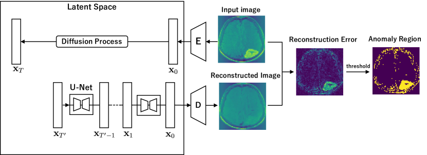
Figure 1: Schematic illustration of the anomaly detection on a brain image dataset using a diffusion model. When a test image, which may contain an abnormal region, is fed into a trained diffusion model, a normal image is generated through the diffusion process and generative process. By initiating the image generation from the middle of the diffusion process (step $T^{\prime}$), a normal image that retains the characteristics of the input image can be generated. By comparing the input image with the normal image, the abnormal region can be identified. In this study, we propose a method called the DMAD-test, which quantifies the statistical significance of the identified abnormal regions in the form of $p$-value. The proposed DMAD-test calculates the $p$-values by incorporating the fact that the abnormal region has been identified by the diffusion model, thus enabling unbiased decision-making.

Problem Formulation

We develop a statistical test to quantify the reliability of the hypotheses generated by the diffusion model. To develop a statistical test, we interpret that an image is considered as a sum of true signal component $\bm{\mu}\in\mathbb{R}^{n}$ and noise component $\bm{\epsilon}\in\mathbb{R}^{n}$. Regarding the true signal component, each pixel can have an arbitrary value without any particular assumption or constraint. On the other hand, regarding the noise component, it is assumed to follow a Gaussian distribution, and their covariance matrix is estimated using normal data different from that used for the training of the diffusion model. Namely, an image with $n$ pixels can be represented as an $n$-dimensional random vector

$$\bm{X}=(X_{1},X_{2},\dots,X_{n})^{\mathrm{T}}=\bm{\mu}+\bm{\epsilon},\;\;\;\bm{\epsilon}\sim\mathcal{N}(\bm{0},\bm{\Sigma})$$ (5)

where $\bm{\mu}\in\mathbb{R}^{n}$ is the unknown true signal vector and $\bm{\Sigma}$ is the covariance matrix, which is known or estimable from external data. In the following, we use capital $\bm{X}$ to emphasize that an image is considered as a random vector, while the observed image is denoted as $\bm{X}^{\rm obs}$.

Let us denote the reconstruction process of the trained diffusion model in Algorithm 1 as the mapping from an input image to the reconstructed image $\mathcal{D}:\mathbb{R}^{n}\ni\bm{X}\rightarrow\mathcal{D}(\bm{X})\in\mathbb{R}^{n}$. The difference between the input image $\bm{X}$ and the reconstructed image $\mathcal{D}(\bm{X})$ indicates the reconstruction error. When identifying anomaly regions based on reconstruction error, it is useful to apply some filter to remove the influence of pixel-wise noise. In this study, we simply used an averaging filter. Let us denote the averaging filter as $\mathcal{F}:\mathbb{R}^{n}\rightarrow\mathbb{R}^{n}$. Then, the process of obtaining the (filtered) reconstruction error is written as

$$E:\mathbb{R}^{n}\ni\bm{X}\mapsto|\mathcal{F}(\bm{X}-\mathcal{D}(\bm{X}))|\in\mathbb{R}^{n},$$ (6)

where absolute value is taken pixel-wise. Anomaly regions are then obtained by applying a threshold to the filtered reconstruction error $E_{i}(\bm{X})$ for each pixel $i\in[n]$. Specifically we define the anomaly region as the set of pixels whose filtered reconstruction error is greater than a given threshold $\lambda\in(0,\infty)$, i.e.,

$$\mathcal{M}_{\bm{X}}=\left\{i\in[n]\mid E_{i}(\bm{X})\geq\lambda\right\}.$$ (7)

Statistical Inference.

In order to quantify the statistical significance of the anomaly regions detected by a diffusion model, let us consider a statistical test with the following null and alternative hypotheses:

$$\begin{gathered}\mathrm{H}_{0}\colon\frac{1}{|\mathcal{M}_{\bm{X}}|}\sum_{i\in\mathcal{M}_{\bm{X}}}\mu_{i}=\frac{1}{|\mathcal{M}_{\bm{X}}^{c}|}\sum_{i\notin\mathcal{M}_{\bm{X}}}\mu_{i}\\ \text{v.s.}\\ \mathrm{H}_{1}\colon\frac{1}{|\mathcal{M}_{\bm{X}}|}\sum_{i\in\mathcal{M}_{\bm{X}}}\mu_{i}\neq\frac{1}{|\mathcal{M}_{\bm{X}}^{c}|}\sum_{i\notin\mathcal{M}_{\bm{X}}}\mu_{i},\end{gathered}$$ (8)

where $\mathrm{H}_{0}$ is the null hypothesis that the mean pixel values are the same between the anomaly regions and other regions, while $\mathrm{H}_{1}$ is the alternative hypothesis that they are different. A reasonable test statistic for the statistical test in (8) is the difference in mean pixel values between the inside and outside of the anomaly region, i.e.,

$$T(\bm{X}) =\frac{1}{|\mathcal{M}_{\bm{X}}|}\sum_{i\in\mathcal{M}_{\bm{X}}}\mu_{i}-\frac{1}{|\mathcal{M}^{c}_{\bm{X}}|}\sum_{i\in\mathcal{M}^{c}_{\bm{X}}}\mu_{i}$$ (9)

$$=\bm{\nu}^{\top}_{\mathcal{M}_{\bm{X}}}\bm{X},$$

where $\bm{\nu}_{\mathcal{M}_{\bm{X}}}=\frac{1}{|\mathcal{M}_{\bm{X}}|}\bm{1}^{n}_{\mathcal{M}_{\bm{X}}}-\frac{1}{|\mathcal{M}^{c}_{\bm{X}}|}\bm{1}^{n}_{\mathcal{M}^{c}_{\bm{X}}}$ is the vector that depends on the anomaly region $\mathcal{M}_{\bm{X}}$ and $\mathbf{1}^{n}_{\mathcal{C}}\in\mathcal{R}^{n}$ is an $n$-dimensional vector whose elements are $1$ if they belong to the set $\mathcal{C}$ and $0$ otherwise.

If we do not account for the fact that the anomaly region is detected by a diffusion model, the distribution of the test statistic would be simply given as $T(\bm{X})\sim\mathcal{N}(0,\bm{\nu}^{\top}_{\mathcal{M}_{\bm{X}}}\bm{\Sigma}\bm{\nu}_{\mathcal{M}_{\bm{X}}})$. In this case, the $p$-values defined as

$$p_{\mathrm{naive}}=\mathbb{P}_{\mathrm{H}_{0}}\left(|T(\bm{X})|>|T(\bm{X}^{\mathrm{obs}})|\right).$$ (10)

would be easily computed by the normality of the test statistic distribution. However, in reality, since the anomaly region is detected by the trained diffusion model, $\bm{\nu}_{\mathcal{M}_{\bm{X}}}$ depends on the data $\bm{X}$, meaning that the sampling distribution of the test statistic is much more complicated. Therefore, if $p_{\mathrm{naive}}$ is used for decision making, the false detection error cannot be properly controlled.

4 Computing Selective $p$-values for Generated Hypotheses

In this section, we introduce selective inference (SI) framework for testing hypotheses generated by diffusion models and propose a method to perform valid hypothesis test.

Conditional Distribution of Test Statistics

Due to the complexity described in the previous section, it is difficult to directly obtain the sampling distribution of $T(\bm{X})$. Then, we consider the sampling distribution of $T(\bm{X})$ conditional on the event that the anomaly region $\mathcal{M}_{\bm{X}}$ is the same as the observed anomaly region $\mathcal{M}_{\bm{X}^{\mathrm{obs}}}$, i.e.,

$$T(\bm{X})\mid\left\{\mathcal{M}_{\bm{X}}=\mathcal{M}_{\bm{X}^{\mathrm{obs}}}\right\}.$$ (11)

In the context of SI, to make the characterization of the conditional sampling distribution manageable, we also incorporate conditioning on the nuisance parameters that is independent of the test statistic. As a result, the calculation of the conditional sampling distribution in SI can be reduced to a one-dimensional search problem in an $n$-dimensional data space. The nuisance parameter $\mathcal{Q}_{\bm{X}}$ is written as

$$\mathcal{Q}_{\bm{X}}=\left(\mathbf{I}_{n}-\frac{\bm{\Sigma}\bm{\nu}_{\mathcal{M}_{\bm{X}}}\bm{\nu}_{\mathcal{M}_{\bm{X}}}^{\top}}{\bm{\nu}^{\top}_{\mathcal{M}_{\bm{X}}}\bm{\Sigma}\bm{\nu}_{\mathcal{M}_{\bm{X}}}}\right)\bm{X}.$$ (12)

The $p$-value calculated from this conditional sampling distribution is called a selective $p$-value. Specifically, the selective $p$-value is defined as

$$p_{\mathrm{selective}}=\mathbb{P}_{\mathrm{H}_{0}}\left(|T(\bm{X})|>|T(\bm{X}^{\mathrm{obs}})|\mid\bm{X}\in\mathcal{X}\right),$$ (13)

where $\mathcal{X}$ is the conditional data space defined as

$$\mathcal{X}=\left\{\bm{X}\in\mathbb{R}^{n}\mid\mathcal{M}_{\bm{X}}=\mathcal{M}_{\bm{X}^{\mathrm{obs}}},\mathcal{Q}_{\bm{X}}=\mathcal{Q}_{\bm{X}^{\mathrm{obs}}}\right\}.$$ (14)

Due to the conditioning on the nuisance parameter $\mathcal{Q}_{\bm{X}}$, the conditional data space $\mathcal{X}$ can be rewritten as

$$\mathcal{X}=\left\{\bm{X}(z)\in\mathbb{R}^{n}\mid\bm{X}(z)=\bm{a}+\bm{b}z,z\in\mathcal{Z}\right\},$$ (15)

where vectors $\bm{a},\bm{b}\in\mathbb{R}^{n}$ are defined as

$$\bm{a}=\mathcal{Q}_{\bm{X}^{\mathrm{obs}}},\;\bm{b}=\frac{\bm{\Sigma}\bm{\nu}_{\mathcal{M}_{\bm{X}^{\mathrm{obs}}}}}{\bm{\nu}^{\top}_{\mathcal{M}_{\bm{X}^{\mathrm{obs}}}}\bm{\Sigma}\bm{\nu}_{\mathcal{M}_{\bm{X}^{\mathrm{obs}}}}},$$ (16)

and the region $\mathcal{Z}$ is defined as

$$\mathcal{Z}=\left\{z\in\mathbb{R}\mid\mathcal{M}_{\bm{a}+\bm{b}z}=\mathcal{M}_{\bm{X}^{\mathrm{obs}}}\right\}.$$ (17)

Let us consider a random variable $Z\in\mathbb{R}$ and its observation $z^{\mathrm{obs}}\in\mathbb{R}$ so that they satisfy $\bm{X}=\bm{a}+\bm{b}Z$ and $\bm{X}^{\mathrm{obs}}=\bm{a}+\bm{b}z^{\mathrm{obs}}$. Then, the selective $p$-value in (13) is re-written as

$$p_{\mathrm{selective}}=\mathbb{P}_{\mathrm{H}_{0}}\left(|Z|>|z^{\mathrm{obs}}|\mid Z\in\mathcal{Z}\right).$$ (18)

Under the null hypothesis $\mathrm{H}_{0}$, the distribution of the unconditional variable $Z$ is $\mathcal{N}(0,\bm{\nu}^{\top}_{\mathcal{M}_{\bm{X}}}\bm{\Sigma}\bm{\nu}_{\mathcal{M}_{\bm{X}}})$. Consequently, given $Z\in\mathcal{Z}$, the conditional random variable $Z$ adheres to a truncated Gaussian distribution. Once the truncated region $\mathcal{Z}$ is identified, computing the selective $p$-value in (18) becomes straightforward. Therefore, the remaining task is the identification of $\mathcal{Z}$.

Over-Conditioning

To compute the truncated region $\mathcal{Z}$, we employ a divide and conquer approach. The basic idea of this approach is to decompose the data space $\mathcal{X}$ into a set of polyhedra by considering additional conditioning, which we refer to as over-conditioning (OC) (Duy and Takeuchi, 2022). It is easy to understood that a polyhedron in the $n$-dimensional data space ${\mathcal{X}}$ corresponds to an interval in the one-dimensional space ${\mathcal{Z}}$. Therefore, we can sequentially examine intervals in the one-dimensional space and check whether the same hypothesis as the observed one is selected. In this study, we show that the filtered reconstruction error $E(\bm{X})$ can be expressed as a piecewise-linear function of $\bm{X}$. By exploiting this, we identify a over-conditioned interval $\mathcal{Z}^{\mathrm{oc}}\subset\mathcal{Z}$.

Identification of $\mathcal{Z}^{\mathrm{oc}}$

Let us write a polyhedron $\mathcal{P}$ composed of piecewise-linear functions as

$$\mathcal{P}_{k}=\left\{\bm{\Delta}_{k}\bm{X}\leq\bm{\delta}_{k}\right\},k\in[K],$$ (19)

where $\bm{\Delta}_{k}$ and $\bm{\delta}_{k}$ for $k\in[K]$ are the coefficient matrix and the constant vector with appropriate dimensions of the $k$-th piecewise-linear function, respectively. Then, a piecewise-linear function $\mathcal{A}(\bm{X})$ is written in the following form:

$$\mathcal{A}(\bm{X})=\begin{cases}\bm{\Psi}_{1}\bm{X}+\bm{\psi}_{2}&\text{if }\bm{X}\in\mathcal{P}_{1},\\ \bm{\Psi}_{2}\bm{X}+\bm{\psi}_{2}&\text{if }\bm{X}\in\mathcal{P}_{2},\\ \hskip 28.45274pt\vdots\\ \bm{\Psi}_{K}\bm{X}+\bm{\psi}_{K}&\text{if }\bm{X}\in\mathcal{P}_{K},\end{cases}$$ (20)

where $\bm{\Psi}_{k}$ and $\bm{\psi}_{k}$ for $k\in[K]$ are the coefficient matrix and the constant vector with appropriate dimensions for the $k$-th polyhedron, respectively. Using the notation in (15), since the input image $\bm{X}(z)$ is restricted on a one-dimensional line, each component of the output of $\mathcal{A}$ is written as

$$\begin{gathered}\mathcal{A}_{i}(\bm{X}(z))=\begin{cases}\kappa^{\mathcal{A}_{i}}_{1}z+\rho^{\mathcal{A}_{i}}_{2}&\text{if }[L^{\mathcal{A}_{i}}_{1},U^{\mathcal{A}_{i}}_{1}],\\ \kappa^{\mathcal{A}_{i}}_{2}z+\rho^{\mathcal{A}_{i}}_{2}&\text{if }[L^{\mathcal{A}_{i}}_{2},U^{\mathcal{A}_{i}}_{2}],\\ \hskip 28.45274pt\vdots\\ \kappa^{\mathcal{A}_{i}}_{K(\mathcal{A}_{i})}z+\rho^{\mathcal{A}_{i}}_{K(\mathcal{A}_{i})}&\text{if }[L^{\mathcal{A}_{i}}_{K(\mathcal{A}_{i})},U^{\mathcal{A}_{i}}_{K(\mathcal{A}_{i})}],\end{cases}\end{gathered}$$ (21)

where $K(\mathcal{A}_{i})$ is the number of polyhedra that depends on $\mathcal{A}_{i}(\bm{X}(z))$, and $\kappa^{\mathcal{A}_{i}}_{k}\in\mathbb{R}$ and $\rho^{\mathcal{A}_{i}}_{k}\in\mathbb{R}$ for $k\in[K(\mathcal{A}_{i})]$ are the coefficient and the constant of the $k$-th polyhedron, respectively. Let $\mathcal{A}_{i}(\bm{X}(z))\geq\lambda$, then interval $z$ can be expressed as

$$z\in\begin{cases}\left[\max\left(L_{k},\left((\lambda-\rho_{k})/\kappa_{k}\right)\right),U_{k}\right]&\text{if }\kappa_{k}>0,\\ \left[L_{k},\min\left(U_{k},\left((\lambda-\rho_{k})/\kappa_{k}\right)\right)\right]&\text{if }\kappa_{k}<0.\end{cases}$$ (22)

We denote the over-conditioned interval as

$$\mathcal{Z}^{\text{oc}}(\bm{a}+\bm{b}z)=\left[L_{z},U_{z}\right].$$ (23)

Piecewise Linearity of Diffusion Models

We now show that the diffusion model mapping $\mathcal{D}$ and then filtered reconstruction error $E$ can be expressed as a piecewise-linear function of $\bm{X}$. To show this, we see that both the diffusion process and generative process of the diffusion model is piecewise-linear function as long as we employ a class of U-Net described below. It is easy to see the piecewise-linearity of the diffusion process as long as we fix the random seed for $\epsilon_{t}$. To make the generative process a piecewise-linear function, we employ a U-Net architecture composed of piecewise-linear components such as ReLU activation function and average pooling. Then, $\epsilon^{(t)}_{\theta}(\mathbf{x}_{t})$ is represented as a piecewise-linear function of $\mathbf{x}_{t}$. Moreover, since $f^{(t)}_{\theta}(\mathbf{x}_{t})$ in (3) is a composite function of $\epsilon^{(t)}_{\theta}(\mathbf{x}_{t})$, it is also a piecewise-linear function. By combining them together, we see that $\mathbf{x}_{t-1}$ is written as a piecewise-linear function of $\mathbf{x}_{t}$. Therefore, the entire decoding process is a piecewise-linear function since it just repeats the above operation multiple times (see Algorithm 1). As a result, the entire mapping ${\mathcal{D}}(\mathbf{X})$ of the diffusion model is a piecewise-linear function of the input image $\bm{X}$. Moreover, since the averaging filter $\mathcal{F}$ and the absolute operation are also piecewise-linear functions, $|\mathcal{F}(\bm{X}-\mathcal{D}(\bm{X}))|(=E(\bm{X}))$ is piecewise-linear. By exploiting this piecewise-linearity, the interval $\mathcal{Z}^{\text{oc}}$ can be computed.

5 DMAD-test

Over-conditioning causes a reduction in power due to excessive conditioning. A technique called Parametric Programming is utilized to explore all intervals along the one-dimensional line, resulting in (17). The truncated region $\mathcal{Z}$ can be represented using $\mathcal{Z}^{\mathrm{oc}}$ as

$$\mathcal{Z}=\bigcup_{z\in\mathbb{R}\mid\mathcal{M}_{\bm{a}+\bm{b}z}=\mathcal{M}_{\bm{X}^{\mathrm{obs}}}}\mathcal{Z}^{\mathrm{oc}}(\bm{a}+\bm{b}z).$$ (24)

The number of $\mathcal{Z}^{\mathrm{oc}}$ is obviously finite due to the finiteness of the number of polyhedra, but for practical purposes it grows exponentially, making it difficult to identify all of them. In many other SI studies, it is known that a search from $z_{\mathrm{min}}=(-10\sigma-|z^{\mathrm{obs}}|)$ to $z_{\mathrm{max}}(=10\sigma+|z^{\mathrm{obs}}|)$ is sufficient for practical use, where $\sigma$ is the standard deviation of the test statistic $T(\bm{X})$. An algorithm for calculating the selective $p$-value via Parametric Programming is summarized in Algorithm 2.

Algorithm 2 Selective $p$-value Computation by Parametric Programming

0:  $\mathbf{X^{\mathrm{obs}}},z_{\mathrm{min}},z_{\mathrm{max}}$ and $z^{\mathrm{obs}}:=T(\bm{X}^{\mathrm{obs}})$

1:  $\mathcal{Z}\leftarrow\emptyset$

2:  Obtain $\mathcal{M}_{\bm{X}^{\mathrm{obs}}}$ by (7)

3:  Compute $\bm{a}$, $\bm{b}$ by (17)

4:  $z\leftarrow z_{\mathrm{min}}$

5:  while $z<z_{\mathrm{max}}$ do

6:     Compute $[L_{z},U_{z}]$ and $\mathcal{M}_{\bm{a}+\bm{b}z}$ by (23) for $z$

7:     if $\mathcal{M}_{\bm{a}+\bm{b}z}=\mathcal{M}_{\bm{X}^{\mathrm{obs}}}$ then

8:        $\mathcal{Z}\leftarrow\mathcal{Z}\cup\left[L_{z},U_{z}\right]$

9:     end if

10:     $z\leftarrow U_{z}+\varepsilon$, where $\varepsilon$ is small positive number.

11:  end while

12:  $p_{\mathrm{selective}}=\mathbb{P}_{\mathrm{H}_{0}}\left(|Z|>|z^{\mathrm{obs}}|\mid Z\in\mathcal{Z}\right)$

12:  $p_{\mathrm{selective}}$

6 Numerical Experiments

We compared the proposed method with the other methods.

Methods for comparison

The details of the methods for comparison are described in Appendix B.1.

• DMAD-test: The proposed method.

• DMAD-test-oc: The proposed method with over-conditioning.

• naive: The naive method.

• bonferroni: Bonferroni correction.

• permutation: Permutation test.

6.1 Experimental Setup

Experiments on the type I error rate and power were conducted with two types of covariance matrices: independent $\bm{\Sigma}=\bm{I}_{n}\in\mathbb{R}^{n\times n}$ and correction $\bm{\Sigma}=(0.5^{|i-j|})_{ij}\in\mathbb{R}^{n\times n}$. The details of the structure of the Diffusion Model we used are shown in Appendix C.1. The Diffusion Models were trained on data tailored to each experimental settings. The Diffusion Models were trained with $T=1000$ and the initial time step of the generation process was set to $T^{\prime}=200$, and the reconstruction was conducted $4$ step samplings. The noise schedule $\beta_{1},\beta_{2},\dots,\beta_{T}$ was set to linear. In this experiment, we aim to generate new images through probabilistic sampling, $\eta$ was set to $1$. We used only normal images for the type I error rate experiments. The synthetic dataset for normal images is generated to follow $\bm{X}=(X_{1},X_{2},\dots,X_{n})\sim\mathcal{N}(\bm{0},\bm{\Sigma})$. we made 1000 normal images for $n\in\left\{64,256,1024,4096\right\}$. In the power experiments, we used only anomaly images. We made 1000 anomaly images $\bm{X}=(X_{1},X_{2},\dots,X_{n})\sim\mathcal{N}(\bm{\mu},\bm{\Sigma})$, where $\mu_{i}=\Delta,\forall i\in\mathcal{S}$, and $\mu_{i}=0,\forall i\in[n]\backslash\mathcal{S}$, where $\mathcal{S}\subset[n]$ is the anomaly region with its position randomly chosen. The image size of the anomaly images was set to 256, with signals $\Delta\in\left\{1,2,3,4\right\}$. The threshold was set to $\lambda=0.8$, and the kernel size of the averaging filter was set to $2$. All experiments were conducted under the significance level $\alpha=0.05$.

6.2 Results

The results of type I error rate comparison are shown in Figure 2. The proposed methods DMAD-test and DMAD-test-oc can control the type I error rate at the significance level $\alpha$, and bonferroni can control the type I error rate below the significance level $\alpha$. In contrast, naive and permutation cannot control the type I error rate. The results of power comparison are shown in Figure 3. Since naive and permutation cannot control the type I error rate, their powers are not considered. Among the methods that can control the type I error rate, the proposed method has the highest power. DMAD-test-oc is over-conditioned and bonferroni is conservative because there are many hypotheses, so they have low power.

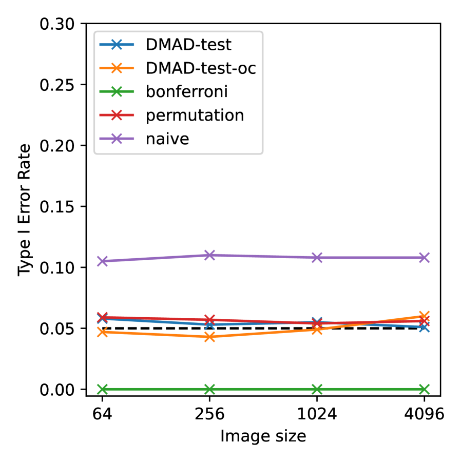
(a) Independence

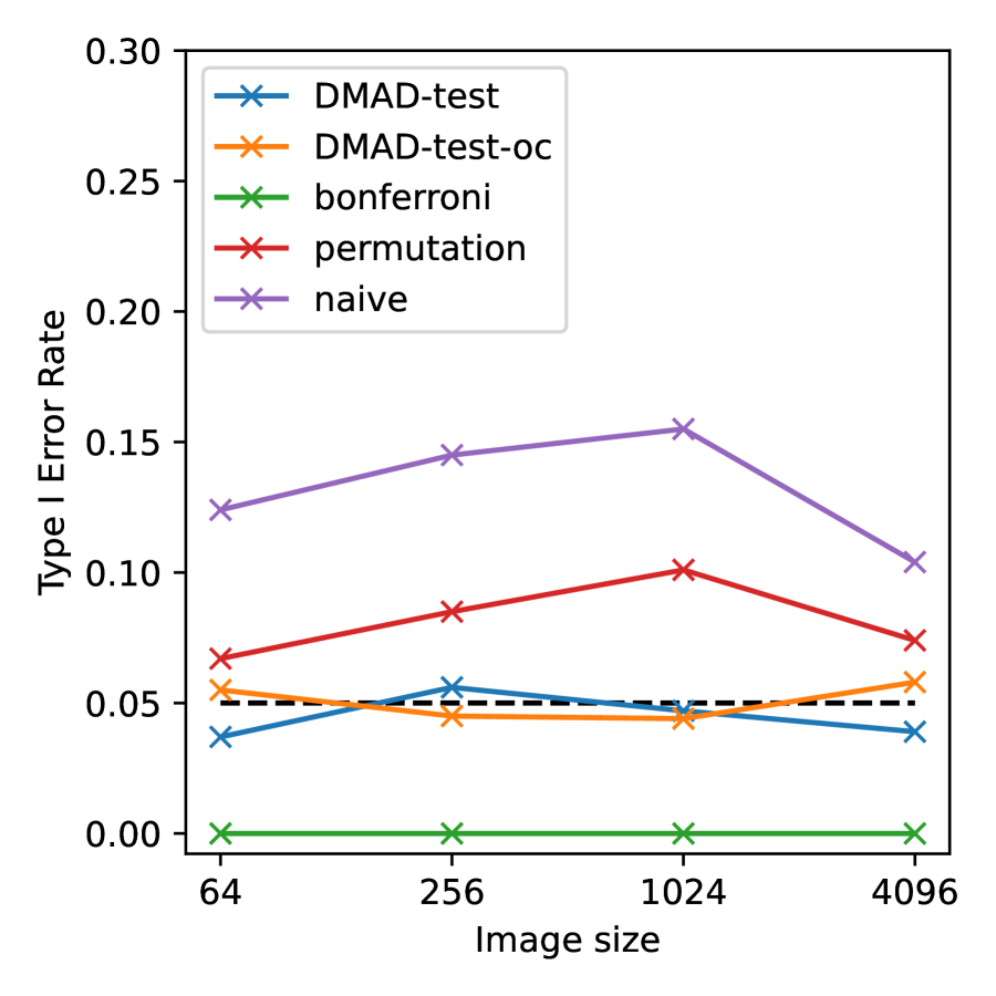
(b) Correlation

Figure 2: Type I Error Rate

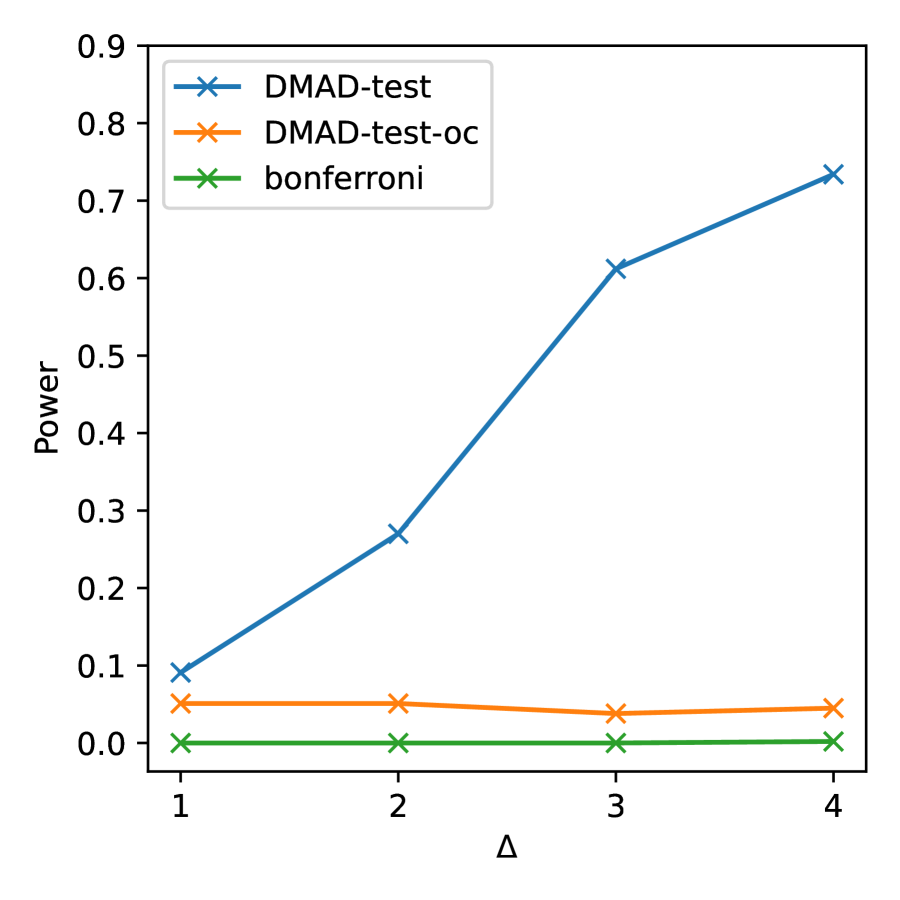
(a) Independence

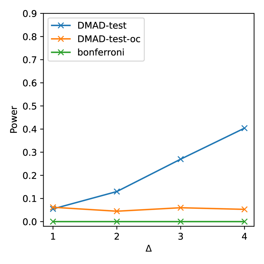
(b) Correlation

Figure 3: Power

6.3 Real Data Experiments

We used the dataset by Buda et al. (2019). This dataset includes brain images with tumors as normal images (939 images) and brain images without tumors as anomaly images (941 images). A random selection of 100 images from the normal images was made to estimate the mean and variance. The remaining images were standardized using the estimated mean and variance, and 750 normal images were extracted for training the diffusion model. The model was trained with $T=1000$ and the initial time step of the generative process was set at $T^{\prime}=330$, with reconstruction performed through 5 step samplings. Experiments were conducted without the averaging filter. we set the threshold $\lambda=0.8$ and the significance level $\alpha=0.05$. Figure 4 and Figure 5 show that, for normal images, the naive method incorrectly detected them as anomaly, whereas the DMAD-test correctly detected them as normal. For anomaly images, the DMAD-test also correctly identifies them as insignificant. This results indicates that the DMAD-test detected anomaly region as statistically significant while avoiding misidentification of normal image as anomaly.

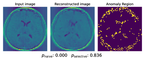
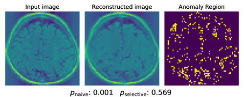
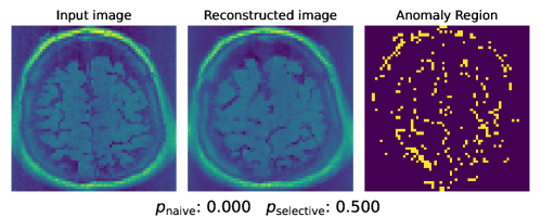
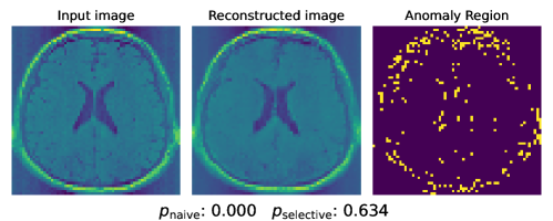
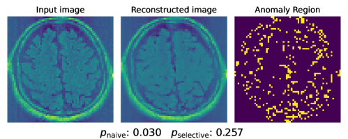
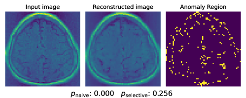
Figure 4: Brain images without tumor

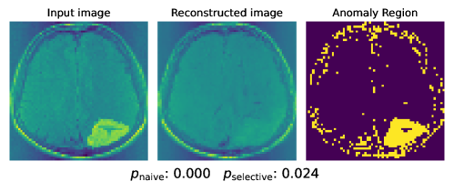
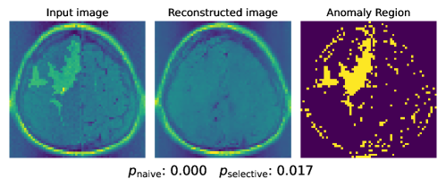
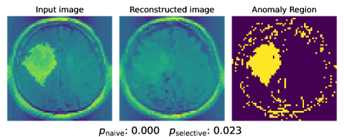
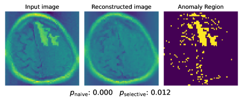
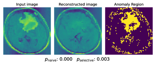
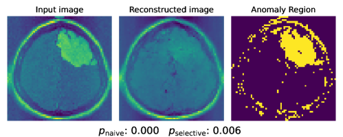
Figure 5: Brain images with tumor

7 Conclusion

In this study, we proposed a statistical test for abnormal regions in medical images detected by a diffusion model. With the proposed DMAD-test, the false detection probability can be controlled with the desired significance level because statistical inference is properly conducted conditional on the fact that the abnormal regions are identified by a diffusion model.

Acknowledgement

This work was partially supported by MEXT KAKENHI (20H00601), JST CREST (JPMJCR21D3, JPMJCR22N2), JST Moonshot R&D (JPMJMS2033-05), JST AIP Acceleration Research (JPMJCR21U2), NEDO (JPNP18002, JPNP20006) and RIKEN Center for Advanced Intelligence Project.

Appendix A Generative Processes

A.1 Accelerated Generative Processes

Methods for accelerating the generative process have been proposed in DDPM, DDIM (Song et al., 2022). When taking a strictly increasing subsequence $\tau$ from $\{1,\cdots,T\}$, it is possible to skip the sampling trajectory from $\mathbf{x}_{\tau_{i}}$ to $\mathbf{x}_{\tau_{i-1}}$. In this case, equations (2) and (4) can be rewritten as

$$\mathbf{x}_{\tau_{i-1}}=\sqrt{\alpha_{\tau_{i-1}}}\left(\frac{\mathbf{x}_{\tau_{i}}-\sqrt{1-\alpha_{\tau_{i}}}\cdot\epsilon^{(\tau_{i})}_{\theta}(\mathbf{x}_{\tau_{i}})}{\sqrt{\alpha_{\tau_{i}}}}\right)+\sqrt{1-\alpha_{\tau_{i-1}}-\sigma_{\tau_{i}}^{2}}\cdot\epsilon_{\theta}^{(\tau_{i})}(\mathbf{x}_{\tau{i}})+\sigma_{\tau_{i}}\epsilon_{\tau_{i}},$$ (25)

where

$$\sigma_{\tau_{i}}=\eta\sqrt{(1-\alpha_{\tau_{i-1}})/(1-\alpha_{\tau_{i}})}\sqrt{1-\alpha_{\tau_{i}}/\alpha_{\tau_{i-1}}}.$$ (26)

Therefore, piecewise-linearity is preserved, making the proposed method DMAD-test applicable.

Appendix B Experimental Details

B.1 Comparison Methods

We compared our proposed method with the following methods:

• DMAD-test: This method uses the parametric programming.

• DMAD-test-oc: This method uses over-conditioning.

• naive: This method uses a conventional $z$-test without any conditioning. The naive $p$-value is calculated as

  $$p_{\mathrm{naive}}=\mathbb{P}_{\mathbb{H}_{0}}\left(|Z|>|z^{\mathrm{obs}}|\right).$$

• permutation: This method uses a permutation test with the steps outlined below:

  • Calculate the observed test statistic $z^{\mathrm{obs}}$ by applying the observated image $\bm{X}^{\mathrm{obs}}$ to the Diffusion Model.

  • For each $i=1,\ldots,B$, compute the test statistic $z^{(i)}$ by applying the permuted image $\bm{X}^{(i)}$ to the Diffusion Model, where $B$ represents the total number of permutations, set to 1,000 in our experiments.

  • The permutation $p$-value is then determined as

    $$p_{\mathrm{permutation}}=\frac{1}{B}\sum_{b\in[B]}\bm{1}\{|z^{(b)}|>|z^{\mathrm{obs}}|\},$$

    where $\bm{1}\{\cdot\}$ denotes the indicator function.

• bonferroni: To control the type I error rate, this method applies the bonferroni correction. Given that the total number of anomaly regions is $2^{n}$, the $p$-value is calculated as ,

  $$p_{\mathrm{bonferroni}}=\min(1,2^{n}\cdot p_{\mathrm{naive}}).$$

This rephrasing aims to maintain the original meaning while enhancing readability and comprehension.

Appendix C Details of the U-Net

C.1 Structure of the U-Net

Figure 6 shows the architecture of the U-Net used in our experiments. The U-Net has three skip connections, and the Encoder and Decoder blocks. The U-Net employs a dense layer for embedding time $t$.

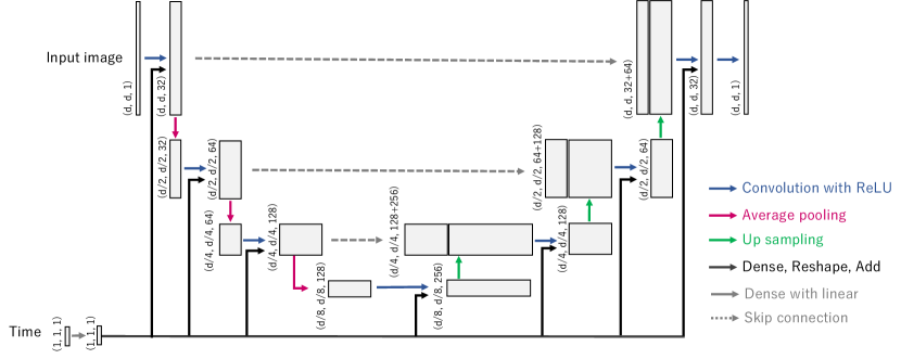
Figure 6: The architecture of the U-Net

References

- Anonymous [2024a] Anonymous. Statistical test for attention maps in vision transformers. Unpublished, 2024a.
- Anonymous [2024b] Anonymous. Statistical test for anomaly detections by variational auto-encoders. Unpublished, 2024b.
- Baur et al. [2021] Christoph Baur, Stefan Denner, Benedikt Wiestler, Nassir Navab, and Shadi Albarqouni. Autoencoders for unsupervised anomaly segmentation in brain mr images: A comparative study. Medical Image Analysis, 69:101952, 2021. ISSN 1361-8415. doi: https://doi.org/10.1016/j.media.2020.101952. URL https://www.sciencedirect.com/science/article/pii/S1361841520303169.
- Benjamini [2020] Yoav Benjamini. Selective inference: The silent killer of replicability. 2020.
- Buda et al. [2019] Mateusz Buda, Ashirbani Saha, and Maciej A. Mazurowski. Association of genomic subtypes of lower-grade gliomas with shape features automatically extracted by a deep learning algorithm. Computers in Biology and Medicine, 109:218–225, 2019. ISSN 0010-4825. doi: https://doi.org/10.1016/j.compbiomed.2019.05.002. URL https://www.sciencedirect.com/science/article/pii/S0010482519301520.
- Chen and Konukoglu [2018] Xiaoran Chen and Ender Konukoglu. Unsupervised detection of lesions in brain MRI using constrained adversarial auto-encoders. In Medical Imaging with Deep Learning, 2018. URL https://openreview.net/forum?id=H1nGLZ2oG.
- Chow et al. [2020] Jun Kang Chow, Zhaoyu Su, Jimmy Wu, Pin Siang Tan, Xin Mao, and Yu-Hsing Wang. Anomaly detection of defects on concrete structures with the convolutional autoencoder. Advanced Engineering Informatics, 45:101105, 2020.
- Duy and Takeuchi [2022] Vo Nguyen Le Duy and Ichiro Takeuchi. More powerful conditional selective inference for generalized lasso by parametric programming. The Journal of Machine Learning Research, 23(1):13544–13580, 2022.
- Duy et al. [2022] Vo Nguyen Le Duy, Shogo Iwazaki, and Ichiro Takeuchi. Quantifying statistical significance of neural network-based image segmentation by selective inference. Advances in Neural Information Processing Systems, 35:31627–31639, 2022.
- Fontanella et al. [2023] Alessandro Fontanella, Grant Mair, Joanna Wardlaw, Emanuele Trucco, and Amos Storkey. Diffusion models for counterfactual generation and anomaly detection in brain images, 2023.
- Ho et al. [2020] Jonathan Ho, Ajay Jain, and Pieter Abbeel. Denoising diffusion probabilistic models. In H. Larochelle, M. Ranzato, R. Hadsell, M.F. Balcan, and H. Lin, editors, Advances in Neural Information Processing Systems, volume 33, pages 6840–6851. Curran Associates, Inc., 2020. URL https://proceedings.neurips.cc/paper_files/paper/2020/file/4c5bcfec8584af0d967f1ab10179ca4b-Paper.pdf.
- Jana et al. [2022] Debasish Jana, Jayant Patil, Sudheendra Herkal, Satish Nagarajaiah, and Leonardo Duenas-Osorio. Cnn and convolutional autoencoder (cae) based real-time sensor fault detection, localization, and correction. Mechanical Systems and Signal Processing, 169:108723, 2022.
- Lee et al. [2016a] Jason D. Lee, Dennis L. Sun, Yuekai Sun, and Jonathan E. Taylor. Exact post-selection inference, with application to the lasso. The Annals of Statistics, 44(3), June 2016a. ISSN 0090-5364. doi: 10.1214/15-aos1371. URL http://dx.doi.org/10.1214/15-AOS1371.
- Lee et al. [2016b] Jason D Lee, Dennis L Sun, Yuekai Sun, and Jonathan E Taylor. Exact post-selection inference, with application to the lasso. The Annals of Statistics, 44(3):907–927, 2016b.
- Miwa et al. [2023] Daiki Miwa, Duy Vo Nguyen Le, and Ichiro Takeuchi. Valid p-value for deep learning-driven salient region. In Proceedings of the 11th International Conference on Learning Representation, 2023.
- Mousakhan et al. [2023] Arian Mousakhan, Thomas Brox, and Jawad Tayyub. Anomaly detection with conditioned denoising diffusion models, 2023.
- Neufeld et al. [2022] Anna C Neufeld, Lucy L Gao, and Daniela M Witten. Tree-values: selective inference for regression trees. Journal of Machine Learning Research, 23(305):1–43, 2022.
- Panigrahi and Taylor [2022] Snigdha Panigrahi and Jonathan Taylor. Approximate selective inference via maximum likelihood. Journal of the American Statistical Association, pages 1–11, 2022.
- Pinaya et al. [2022] Walter H. L. Pinaya, Mark S. Graham, Robert Gray, Pedro F. da Costa, Petru-Daniel Tudosiu, Paul Wright, Yee H. Mah, Andrew D. MacKinnon, James T. Teo, Rolf Jager, David Werring, Geraint Rees, Parashkev Nachev, Sebastien Ourselin, and M. Jorge Cardoso. Fast unsupervised brain anomaly detection and segmentation with diffusion models. In Linwei Wang, Qi Dou, P. Thomas Fletcher, Stefanie Speidel, and Shuo Li, editors, Medical Image Computing and Computer Assisted Intervention – MICCAI 2022, pages 705–714, Cham, 2022. Springer Nature Switzerland. ISBN 978-3-031-16452-1.
- Sanchez-Lengeling and Aspuru-Guzik [2018] Benjamin Sanchez-Lengeling and Alán Aspuru-Guzik. Inverse molecular design using machine learning: Generative models for matter engineering. Science, 361(6400):360–365, 2018.
- Schneider et al. [2020] Petra Schneider, W Patrick Walters, Alleyn T Plowright, Norman Sieroka, Jennifer Listgarten, Robert A Goodnow Jr, Jasmin Fisher, Johanna M Jansen, José S Duca, Thomas S Rush, et al. Rethinking drug design in the artificial intelligence era. Nature Reviews Drug Discovery, 19(5):353–364, 2020.
- Song et al. [2022] Jiaming Song, Chenlin Meng, and Stefano Ermon. Denoising diffusion implicit models, 2022.
- Song and Ermon [2019] Yang Song and Stefano Ermon. Generative modeling by estimating gradients of the data distribution. Advances in neural information processing systems, 32, 2019.
- Suzumura et al. [2017] Shinya Suzumura, Kazuya Nakagawa, Yuta Umezu, Koji Tsuda, and Ichiro Takeuchi. Selective inference for sparse high-order interaction models. In Proceedings of the 34th International Conference on Machine Learning-Volume 70, pages 3338–3347. JMLR. org, 2017.
- Tanizaki et al. [2020] Kosuke Tanizaki, Noriaki Hashimoto, Yu Inatsu, Hidekata Hontani, and Ichiro Takeuchi. Computing valid p-values for image segmentation by selective inference. In Proceedings of the IEEE/CVF Conference on Computer Vision and Pattern Recognition, pages 9553–9562, 2020.
- Tian and Taylor [2018] Xiaoying Tian and Jonathan Taylor. Selective inference with a randomized response. The Annals of Statistics, 46(2):679–710, 2018.
- Tibshirani et al. [2016] Ryan J Tibshirani, Jonathan Taylor, Richard Lockhart, and Robert Tibshirani. Exact post-selection inference for sequential regression procedures. Journal of the American Statistical Association, 111(514):600–620, 2016.
- Wang et al. [2023] Hanchen Wang, Tianfan Fu, Yuanqi Du, Wenhao Gao, Kexin Huang, Ziming Liu, Payal Chandak, Shengchao Liu, Peter Van Katwyk, Andreea Deac, et al. Scientific discovery in the age of artificial intelligence. Nature, 620(7972):47–60, 2023.
- Wolleb et al. [2022] Julia Wolleb, Florentin Bieder, Robin Sandkühler, and Philippe C. Cattin. Diffusion models for medical anomaly detection. In Linwei Wang, Qi Dou, P. Thomas Fletcher, Stefanie Speidel, and Shuo Li, editors, Medical Image Computing and Computer Assisted Intervention – MICCAI 2022, pages 35–45, Cham, 2022. Springer Nature Switzerland. ISBN 978-3-031-16452-1.
- Wyatt et al. [2022] Julian Wyatt, Adam Leach, Sebastian M. Schmon, and Chris G. Willcocks. Anoddpm: Anomaly detection with denoising diffusion probabilistic models using simplex noise. In Proceedings of the IEEE/CVF Conference on Computer Vision and Pattern Recognition (CVPR) Workshops, pages 650–656, June 2022.
- Yamada et al. [2018] Makoto Yamada, Yuta Umezu, Kenji Fukumizu, and Ichiro Takeuchi. Post selection inference with kernels. In International conference on artificial intelligence and statistics, pages 152–160. PMLR, 2018.