Reinforcement Learning as a Parsimonious Alternative to Prediction Cascades:
A Case Study on Image Segmentation

Abstract

Deep learning architectures have achieved state-of-the-art (SOTA) performance on computer vision tasks such as object detection and image segmentation. This may be attributed to the use of over-parameterized, monolithic deep learning architectures executed on large datasets. Although such large architectures lead to increased accuracy, this is usually accompanied by a larger increase in computation and memory requirements during inference. While this is a non-issue in traditional machine learning (ML) pipelines, the recent confluence of machine learning and fields like the Internet of Things (IoT) has rendered such large architectures infeasible for execution in low-resource settings. For some datasets, large monolithic pipelines may be overkill for simpler inputs. To address this problem, previous efforts have proposed decision cascades where inputs are passed through models of increasing complexity until desired performance is achieved. However, we argue that cascaded prediction leads to sub-optimal throughput and increased computational cost due to wasteful intermediate computations. To address this, we propose PaSeR (Parsimonious Segmentation with Reinforcement Learning) a non-cascading, cost-aware learning pipeline as an efficient alternative to cascaded decision architectures. Through experimental evaluation on both real-world and standard datasets, we demonstrate that PaSeR achieves better accuracy while minimizing computational cost relative to cascaded models. Further, we introduce a new metric IoU/GigaFlop to evaluate the balance between cost and performance. On the real-world task of battery material phase segmentation, PaSeR yields a minimum performance improvement of $\mathbf{174}\%$ on the IoU/GigaFlop metric with respect to baselines. We also demonstrate PaSeR’s adaptability to complementary models trained on a noisy MNIST dataset, where it achieved a minimum performance improvement on IoU/GigaFlop of $\mathbf{13.4}\%$ over SOTA models. Code and data are available at https://github.com/scailab/paser.

Introduction

Figure 1: Performance w.r.t IoU/GigaFlop metric (higher is better) of SOTA models and our proposed PaSeR model on the battery material phase segmentation task.

Recent advances in deep learning (DL) and the internet-of-things (IoT) have led to the burgeoning application of DL in manufacturing pipelines (Hussain et al. 2020; Meng et al. 2020; Mohammadi et al. 2018; Tang et al. 2017). In many such applications, ML / DL models are often deployed on devices with low memory and computational capabilities (edge) in conjunction with DL models that are deployed in less constrained environments (fog, cloud). These edge-fog-cloud (EFC) systems are commonly used in areas such as smart manufacturing (Chen et al. 2018a) and healthcare (Mutlag et al. 2021) where precision machines such as electrocardiograms collect and preprocess high density data while integrating with a local computer as well as cloud based resources to accurately and efficiently provide critical information. Although the fog and cloud environments enable the deployment of larger DL models, querying them is costly (due to communication network and model latency). Hence, such real-world contexts require a high-throughput pipeline to balance task accuracy and computational cost.

A popular solution to deal with this problem is the I Don’t Know (IDK) Cascade (Wang et al. 2017) in which models of increasing complexity (starting with the least cost model) are sequentially queried until a model yields a prediction exceeding a preset confidence threshold. Multi-exit models (Kouris et al. 2022) follow a similar cascading architecture but require a potentially costly neural architecture search during training. We argue that such pipelines, although well-motivated, lead to high computational costs due to excess computations incurred as a function of the sequential cascading constraint. In this paper, we argue that reinforcement learning (RL) can be employed as an effective substitute to circumvent the cascading restriction. We employ RL to directly select which of a set of models to query with a particular input such that the learned policy maximizes task performance while minimizing computational cost. To this end, we propose the PaSeR framework and demonstrate its performance on the challenging task of battery material phase segmentation.

Application Background. Lithium-ion batteries are extensively used in many industrial applications, (e.g., smartphones, laptops, and electric vehicles) due to their efficient energy storage capability. The electrode coatings of these batteries consist of composite active materials (e.g., Lithium, Nickel, Manganese) and a polymeric binder (Carbon). The microstructure of these composite electrode coatings consists of the spatial distribution of active and binder materials. The physical parameters of a microstructure, (e.g., homogeneity of coating thickness, porosity) influence battery performance. Resolving the locations of the active and binder materials and their phase transitions (i.e., the task of battery material phase segmentation) can help deduce these physical parameters, thereby providing an understanding of phenomena like battery degradation. Existing techniques to address this problem use expensive high-resolution X-ray computed tomography images (Lu et al. 2020). Low-resolution (low-res) microtomography images have also been used, but they cannot readily distinguish between spatial distributions of the composite active materials. Recently, DL segmentation models like MatPhase by  (Tabassum et al. 2022) have been developed to identify (pixel-wise) these composite materials and their phase transitions from low-res images, however, these approaches are computationally expensive to execute.

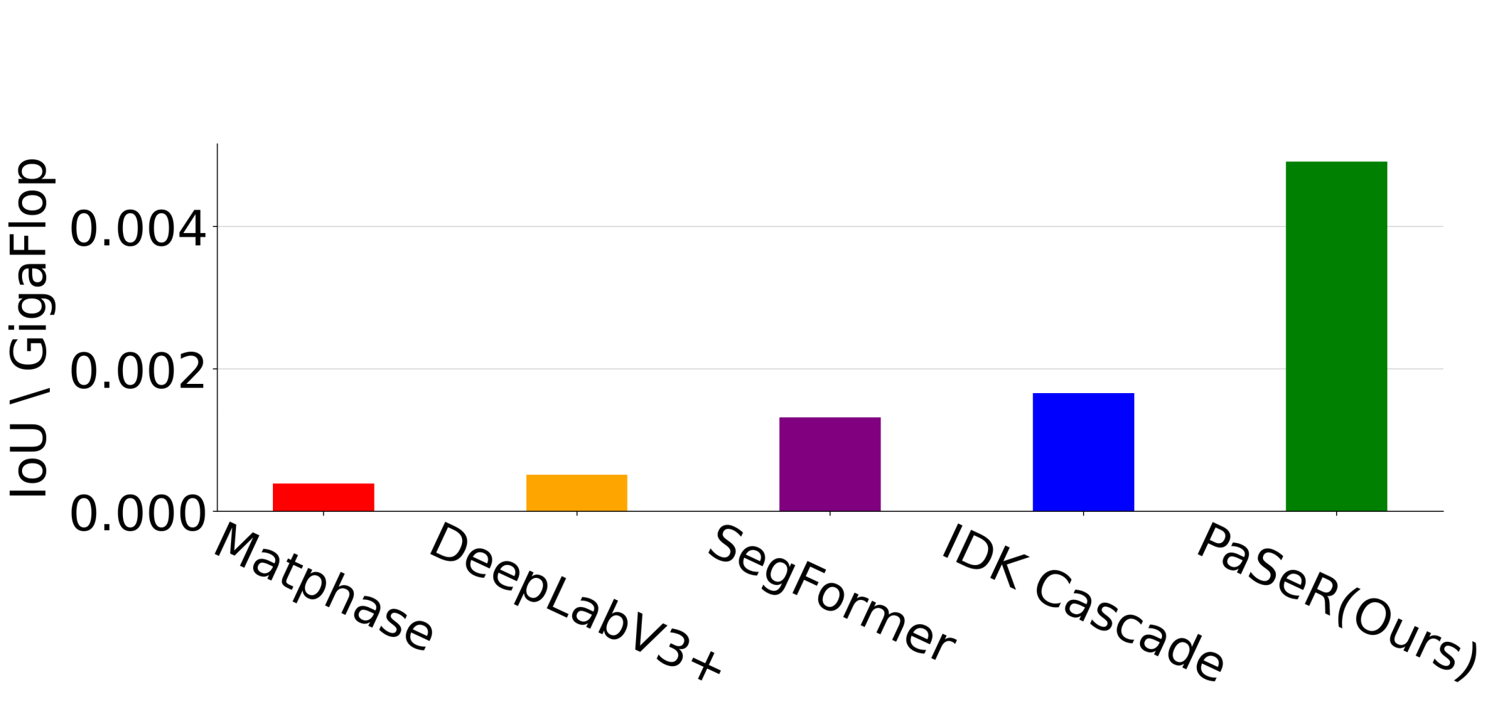
In this context, we propose PaSeR as a low-cost but effective and robust solution to address the task of battery material segmentation from low-res microtomography images. Our contributions are as follows: (C1) We develop a novel computationally parsimonious DL framework (employing reinforcement learning with cost-aware rewards) to balance cost with task performance. (C2) Through qualitative and quantitative experiments, we demonstrate that PaSeR yields competitive performance with SOTA models on the battery material phase segmentation task while also being the most computationally efficient. (C3) We demonstrate the effectiveness of the learned RL policy in unseen (noisy) contexts as well as with task models having complementary strengths. (C4) Finally, we introduce a novel metric called IoU per GigaFlop (IoU/GigaFlop) which measures the segmentation performance obtained per GigaFlop of computation expended, an effective metric for evaluating such low-cost learning pipelines (see Fig. 1).

Related Work

We review two areas of research related to our work, low-cost ML and image segmentation models.

Low-Cost & Tiny ML. There have been many past efforts to develop low-cost DL pipelines for use in low memory, low storage, high-throughput IoT contexts. Knowledge distillation (KD) and employing decision cascades are two popular approaches in this context. While the primary goal of KD (Hinton, Vinyals, and Dean 2015; Gou et al. 2021; Phuong and Lampert 2019) is to learn smaller models to mimic larger models, this goal isn’t fully aligned with the scope of the current work, which is to learn optimal decision pipelines to create a low cost, high performance ML by incorporating multi-models. However, the other research thread of employing decision cascades is directly relevant to our work. Decision Cascades, originally introduced in (Cai, Saberian, and Vasconcelos 2015; Angelova et al. 2015) were recently re-popularized by the work of IDK Cascades (Wang et al. 2017). The IDK cascade framework imposes a sequential model architecture, where each model is queried in order of increasing complexity until prediction confidence exceeds a threshold. Yet another paradigm of Tiny-ML (Rajapakse, Karunanayake, and Ahmed 2023; Ren, Anicic, and Runkler 2022) also aims to develop ML models but with the goal of deploying them on extremely low-cost hardware devices. Our goal is aligned with but complementary to this as our proposed decision pipeline can be employed with such low-cost models along with higher-cost models (on the cloud) to maximize performance and minimize computational cost.

Image Segmentation. The field of image segmentation has also seen many successes in multiple domains  (Chen et al. 2017; Li et al. 2018; Chen et al. 2019) with popular architectures like the U-Net (Ronneberger, Fischer, and Brox 2015) and the recent Segment Anything (Kirillov et al. 2023) foundation model. Our PaSeR framework is flexible enough to incorporate any of these SOTA segmentation models as we have developed a decision pipeline that can leverage multiple models to maximize performance on a target task while minimizing computational cost. Finally, efforts in intelligent data sampling (Uzkent, Yeh, and Ermon 2020; Uzkent and Ermon 2020) which may possess a motivation in terms of employing RL for maximal task performance at minimal cost, differ in the actual application of the RL pipeline and learning task.

Problem Formulation

Figure 2: Overview of PaSeR. The small UNet ($f_{0}$) yields the segmentation ($\hat{\mathbf{y}}_{f_{0}}$) and corresponding entropy map $\mathbf{e}_{f_{0}}$ conditioned on the whole input image ($\mathbf{x}$). Then, $\mathbf{x}$ is divided into ‘P’ equal sized patches. The RL policy directs each patch $\mathbf{x}^{(p)}$ of $\mathbf{x}$ to one of $f_{0},f_{1},f_{2}$ to maximize reward. Based on the RL actions, models $f_{1}$ and $f_{2}$ yield predictions for the corresponding image patch. All the predicted patches are then aggregated to yield the final segmentation.

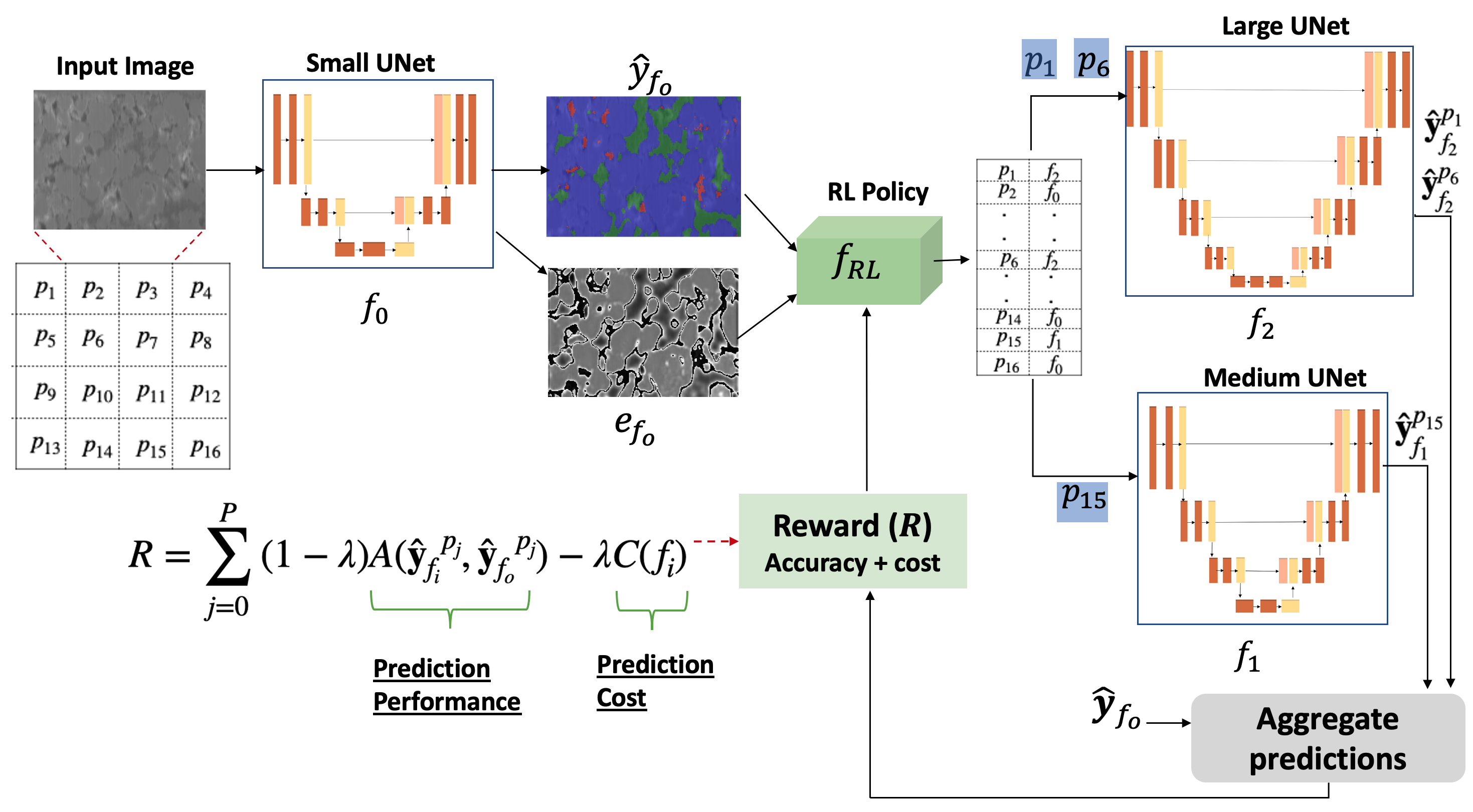
In this work, our goal is to develop a learnable decision pipeline that is computationally parsimonious (i.e., minimizes wasteful computations) and also yields competitive performance (compared to SOTA models) on the target task. To develop such a decision pipeline, we leverage reinforcement learning (RL). Specifically, we propose the PaSeR framework (see Fig. 2 for architecture details) composed of an RL policy model $f_{RL}$, a small/efficient task model $f_{0}$, and $m$ large task models $\{f_{1},\ldots,f_{m}\}$. In this paper, we demonstrate the performance of PaSeR in the context of image segmentation. Algorithm 1 outlines the training procedure of PaSeR in the context of our target task (i.e., image segmentation), but we note that PaSeR is task independent and can be applied to other learning contexts with a few appropriate modifications. Code and data are available at https://github.com/scailab/paser.

Data: $\mathcal{D}_{PT},\mathcal{D}_{RL},\mathcal{D}_{FT}\quad\textbf{Parameters: }\mathbf{\theta}_{f_{RL}},\mathbf{\theta}_{f_{0}},\ldots,\mathbf{\theta}_{f_{m}}\quad\textbf{Hyp: }\lambda,\eta,\beta$

Models: RL policy $f_{RL}$, small/efficient model $f_{0}$ and $m$ large task models $\{f_{1},\ldots,f_{m}\}$

for $f_{i}\in\{f_{1},\ldots,f_{m}\}$                       # Pretrain each large task model

1 do

       for $\mathbf{x}^{(p)},\mathbf{y}^{(p)}\in\mathscr{P}(\mathcal{D}_{PT})$              # For each data point in pre-training dataset

2       do

             $\hat{\mathbf{y}}_{f_{i}}^{(p)},\hat{\mathbf{z}}_{f_{i}}^{(p)}\leftarrow f_{i}(\mathbf{x}^{(p)})$              # Get task predictions and logits from model $f_{i}$

             $l\leftarrow\mathcal{L}(\hat{\mathbf{z}}_{f_{i}}^{(p)},\mathbf{y}^{(p)})$                  # Compute loss (cross entropy)

             $\mathbf{\theta}_{f_{i}}\leftarrow\mathbf{\theta}_{f_{i}}-\eta\nabla_{\mathbf{\theta}_{f_{i}}}l$                # Update model parameters

3            

4       end for

5      

6 end for

for $\mathbf{x},\mathbf{y}\in\mathcal{D}_{PT}$                               # Pretrain small/efficient model with KD loss

7 do

       $\hat{\mathbf{y}}_{f_{0}},\hat{\mathbf{z}}_{f_{0}}\leftarrow f_{0}(\mathbf{x})$                       # Get small model ($f_{0}$) prediction

       $\hat{\mathbf{y}}_{f_{m}},\hat{\mathbf{z}}_{f_{m}}\leftarrow f_{m}(\mathbf{x})$                     # Get largest model prediction

       $l\leftarrow\mathcal{L}(\hat{\mathbf{z}}_{f_{0}},\mathbf{y})+\beta\mathcal{L}_{KD}(\hat{\mathbf{z}}_{f_{0}},\hat{\mathbf{z}}_{f_{m}})$   # Compute loss with KD

       $\mathbf{\theta}_{f_{0}}\leftarrow\mathbf{\theta}_{f_{0}}-\eta\nabla_{\mathbf{\theta}_{f_{0}}}l$                     # Update model parameters

8      

9 end for

for $\mathbf{x},\mathbf{y}\in\mathcal{D}_{RL}$                                # Train RL policy model

10 do

       $\hat{\mathbf{y}}_{f_{0}},\mathbf{e}_{f_{0}}\leftarrow f_{0}(\mathbf{x})$                        # Get small model prediction and entropy

       $\mathbf{s}\leftarrow f_{RL}(\hat{\mathbf{y}}_{f_{0}},\mathbf{e}_{f_{0}})$                      # Get probabilities of actions from RL model

       $\mathbf{a}\sim\pi_{RL}(\mathcal{A}\mid\mathbf{s})$                         # Sample action from RL policy distribution

       for $a_{p}\in\mathbf{a}$                                 # For each model and patch in action

11       do

             $\hat{\mathbf{y}}_{a_{p}}^{(p)}\leftarrow f_{a_{p}}(\mathbf{x}^{(p)})$                                # Get model prediction

             $R\mathrel{{+}{=}}(1-\lambda)A(\hat{\mathbf{y}}_{f_{a_{p}}}^{(p)},\hat{\mathbf{y}}_{f_{0}}^{(p)})-\lambda C(f_{a_{p}})$     # Compute accuracy+cost-based reward

12            

13       end for

      $\nabla_{\mathbf{\theta}_{RL}}J=\mathbb{E}[\nabla_{\mathbf{\theta}_{RL}}\log\pi_{RL}(\mathcal{A}|s)*R]$             # Compute policy gradient

       $\mathbf{\theta}_{f_{RL}}\leftarrow\mathbf{\theta}_{f_{RL}}-\eta\nabla_{\mathbf{\theta}_{f_{RL}}}J(\pi_{RL})$                    # Update RL model

14      

15 end for

for $\mathbf{x},\mathbf{y}\in\mathcal{D}_{FT}$                                # Finetune models

16 do

       Repeat Lines: 5-7 for each large model

       Repeat Lines: 19-28 for RL model

17      

18 end for

Algorithm 1 PaSeR Algorithm

Segmentation Model Pretraining. At the outset of our training procedure, we split the training data into three equal subsets: $\mathcal{D}_{PT},\mathcal{D}_{RL},\mathcal{D}_{FT}$. Each subset is comprised of image instances and pixel labels $(\mathbf{x},\mathbf{y})$ where $\mathbf{x}\in\mathbb{R}^{C\times H\times W}$ and $\mathbf{y}\in\mathbb{R}^{1\times H\times W}$. Using the pretraining subset $\mathcal{D}_{PT}$, we train the $m$ large segmentation models $f_{1},\ldots,f_{m}$ first by splitting each image $\mathbf{x}$ into $P$ equal size patches (in our case $P=16$) with the help of a patchification function $\mathscr{P}(\cdot)$ where $\mathbf{x}^{(p)}$ denotes the $p^{th}$ patch. These patches are passed as inputs to each model while optimizing cross entropy loss $\mathcal{L}(\hat{\mathbf{z}}^{(p)},\mathbf{y}^{(p)})$ between the prediction logits $\hat{\mathbf{z}}^{(p)}$ and ground truth $\mathbf{y}^{(p)}$. Once models $f_{1},\dots,f_{m}$, are pre-trained, the smallest model, $f_{0}$ is pre-trained using $\mathcal{D}_{PT}$ on the full image (i.e., no patchification). In addition to using the cross entropy loss $\mathcal{L}(\hat{\mathbf{z}},\mathbf{y})$ we also use a knowledge distillation (KD) loss (Hinton, Vinyals, and Dean 2015; Kim et al. 2021) between the outputs of the largest model $f_{m}$ and the small model $f_{0}$. We define the KD loss function in Eq. 1.

$$\mathcal{L}_{KD}=\frac{1}{|\mathcal{D}_{PT}|}\sum_{j=1}^{|\mathcal{D}_{PT}|}\left(\hat{\mathbf{z}}^{(p)}_{{f_{0}},j}-\hat{\mathbf{z}}^{(p)}_{{f_{m}},j}\right)^{2}$$ (1)

The term $\hat{\mathbf{y}}^{(p)}_{f_{0},j}$ indicates the segmentation predictions for patch $p$ of instance $j$ yielded by model $f_{0}$. $\hat{\mathbf{y}}^{(p)}_{f_{m},j}$ is the corresponding prediction yielded by model $f_{m}$. This loss encourages outputs of $f_{0}$ to be closer to the largest model $f_{m}$, thereby transferring information from the representations learned by $f_{m}$ to $f_{0}$ improving its performance without increasing its size.

RL Training. We incorporate reinforcement learning as the decision paradigm to develop a compute-efficient segmentation pipeline. Specifically, our RL policy is conditioned upon states $\mathbf{s}$, constituted by the image segmentation $\hat{\mathbf{y}}_{f_{0}}$ and entropy maps $\mathbf{e}_{f_{0}}$ of the smallest model $f_{0}$ to output an action which specifies a set of patch and model pairs for each image to be passed upstream to more sophisticated models in the pipeline. States are of the form $(\hat{\mathbf{y}}_{f_{0}},\mathbf{e}_{f_{0}})$ and actions are defined as $\mathbf{a}\in\{0,\ldots,m\}^{P}$. We define the patch-model selection policy as ${\pi_{RL}(\mathbf{a}\mid\mathbf{s})=p(\mathbf{a}\mid f_{RL}(\hat{\mathbf{y}}_{f_{0}},\mathbf{e}_{f_{0}};\mathbf{\theta}_{f_{RL}}))}$. Here the policy network $f_{RL}$ parameterizes the action distribution $p$, which in our case is a categorical distribution with probabilities ${\mathbf{s}\in\{s_{f_{0}},\ldots,s_{f_{m}}\}^{P}:s_{f_{i}}>0,\,\,\sum_{i=0}^{m}s_{f_{i}}=1}$. The entropy $\mathbf{e}_{f_{0}}$ is calculated using Monte Carlo dropout (Gal and Ghahramani 2016), but note that other methods for uncertainty quantification can also be supported by PaSeR.

Using probabilities $\mathbf{s}$, we sample from a categorical distribution to obtain an action $\mathbf{a}\in\{0,\ldots,m\}^{P}$. For example, if $\mathbf{a}_{k}$ = 2 for some index $k$ of $\mathbf{a}$, this indicates that $f_{RL}$ has chosen the $k^{th}$ patch to be directed to model $f_{2}$ for segmentation. Using the sampled action, we pass each patch to its respective model and compute a reward. The reward function is detailed in Eq. 2 and is based on the difference in prediction performance $A$ between the large and small model predictions, $\hat{\mathbf{y}}_{f_{a_{p}}},\hat{\mathbf{y}}_{f_{0}}$, as well as a computational cost penalty term $C$. The action $\mathbf{a}$ defines the models run on each patch.

$$R(\mathbf{a}=\{a_{1},\ldots,a_{P}\})=\sum_{p=0}^{P}(1-\lambda)A(\hat{\mathbf{y}}_{f_{a_{p}}}^{(p)},\hat{\mathbf{y}}_{f_{0}}^{(p)})-\lambda C(f_{a_{p}})$$ (2)

For our experiments in segmentation we use the difference in mean intersection over union (IoU) as our measure of prediction performance: ${A(\hat{\mathbf{y}}_{f_{i}}^{(p)},\hat{\mathbf{y}}_{f_{0}}^{(p)})=IoU(\hat{\mathbf{y}}_{f_{i}}^{(p)})-IoU(\hat{\mathbf{y}}_{f_{0}}^{(p)})}$. Note that in Eq. 2, the cost parameter $\lambda$ parameterizes a convex combination of accuracy and computational cost to provide a simple way to control the influence of each component on the RL policy reward. We design a cost function $C$ in Eq. 3 with range $(0,1)$ as the ratio of the number of learnable parameters in a model to the total number of parameters in all models $\{f_{0},\dots,f_{m}\}$.

$$C(f_{i})=\frac{\text{numParams}(f_{i})}{\sum_{j=1}^{m}\text{numParams}(f_{j})}$$ (3)

Using the reward value $R$, we compute the policy gradient (Sutton et al. 1999) $\nabla_{\mathbf{\theta}_{f_{RL}}}J=\mathbb{E}[\nabla_{\mathbf{\theta}_{f_{RL}}}\log\pi_{RL}(\mathbf{a}\mid\mathbf{s})*R]$ and update the parameters $\mathbf{\theta}_{RL}$ of the RL policy.

Fine-Tuning. The final step of PaSeR is fine-tuning. Here, we jointly update the large models and RL model. The joint training helps the large segmentation models improve their performance on the inputs being directed to them by the RL policy while also further personalizing the RL policy to discern the strengths and weaknesses of each constituent segmentation model for each input patch.

Experimental Setup

We train three UNet segmentation models $f_{0},f_{1},f_{2}$ with 16571, 1080595, and 17275459 parameters respectively on $\mathcal{D}_{PT}$ for 200 epochs, followed by training our RL model $f_{RL}$ with 14736 parameters on $\mathcal{D}_{RL}$ for 200 epochs. Finally, we fine-tune all models on $\mathcal{D}_{FT}$ for 200 epochs. PaSeR trains with a batch size of 32 using the Adam optimizer (Kingma and Ba 2014) with $\eta=0.0001$. In our battery segmentation experiment we set $\beta=0.01$ using grid search and $\lambda=0.5$ which corresponds to an even balance between performance and cost. For the noisy MNIST dataset we set $\lambda=0$, see section R4. Adaptability to Complementary Models for more details.

Baselines

We compare PaSeR to six baselines with complementary strengths to illustrate how we improve upon each of these baselines in either IoU performance and/or IoU per GigaFlop efficiency. (1) IDK-Cascade (Wang et al. 2017): We implement the IDK-Cascade model with a cost aware cascade using the same segmentation models in PaSeR. For the IDK loss and cost function we use cross entropy loss and our previously defined cost function (Eq. 3), while tuning this baseline with an exhaustive grid search. (2) PaSeR-RandPol.: We setup PaSeR with a random policy for actions drawn uniformly from a categorical distribution. We call this method PaSeR-RandPol. (3) MatPhase (Tabassum et al. 2022): We also compare PaSeR to a state of the art (SOTA) model specialized for the task of battery material phase segmentation. The MatPhase model is an ensemble method which combines UNet segmentation models with pixel level IDK classification and a convolutional neural network. (4) DeepLabV3+ (Chen et al. 2018b): To put PaSeR in context with modern DL models, we compare it to DeepLabV3+, a SOTA segmentation model which uses atrous convolutions alongside an encoder-decoder. (5) SegFormer (Xie et al. 2021): We also compare our method to SegFormer, a recent SOTA segmentation model which combines transformers with small multi-layer perceptron decoders. (6) EfficientViT (Cai et al. 2022): We also compare to the lightweight EfficientViT, which uses linear attention.

Evaluation Metrics

(1) Intersection-Over-Union (IoU): We employ IoU (aka. Jaccard index), a popular and effective metric used to evaluate performance on image segmentation tasks. (2) Flops (F): We profile the number of floating point operations per instance for PaSeR and baselines in inference mode when run on the full test set. This gives us the raw computational cost of each model. (3) IoU Per GigaFlop ($\,\frac{\mathrm{IoU}}{\mathrm{GigaFlop}}\,$): While Flops measures compute required per model, we introduce a new metric called IoU per GigaFlop which is defined by the ratio $\frac{\text{IoU}}{\text{GigaFlop}}$. This metric enables a unified understanding of performance effectiveness and computational cost.

Dataset Description

Battery Material Phase Segmentation. Our battery material phase segmentation dataset consists of 1,330 images (1270 training images, 20 validation, and 40 test images) obtained from low-res microtomography (inputs), each of size $(224,256)$ along with pixel level labels of 3 classes (obtained from high-res computational tomography): pore, carbon, and nickel. We split these images into 16 equal size patches of size $(56,64)$ each.

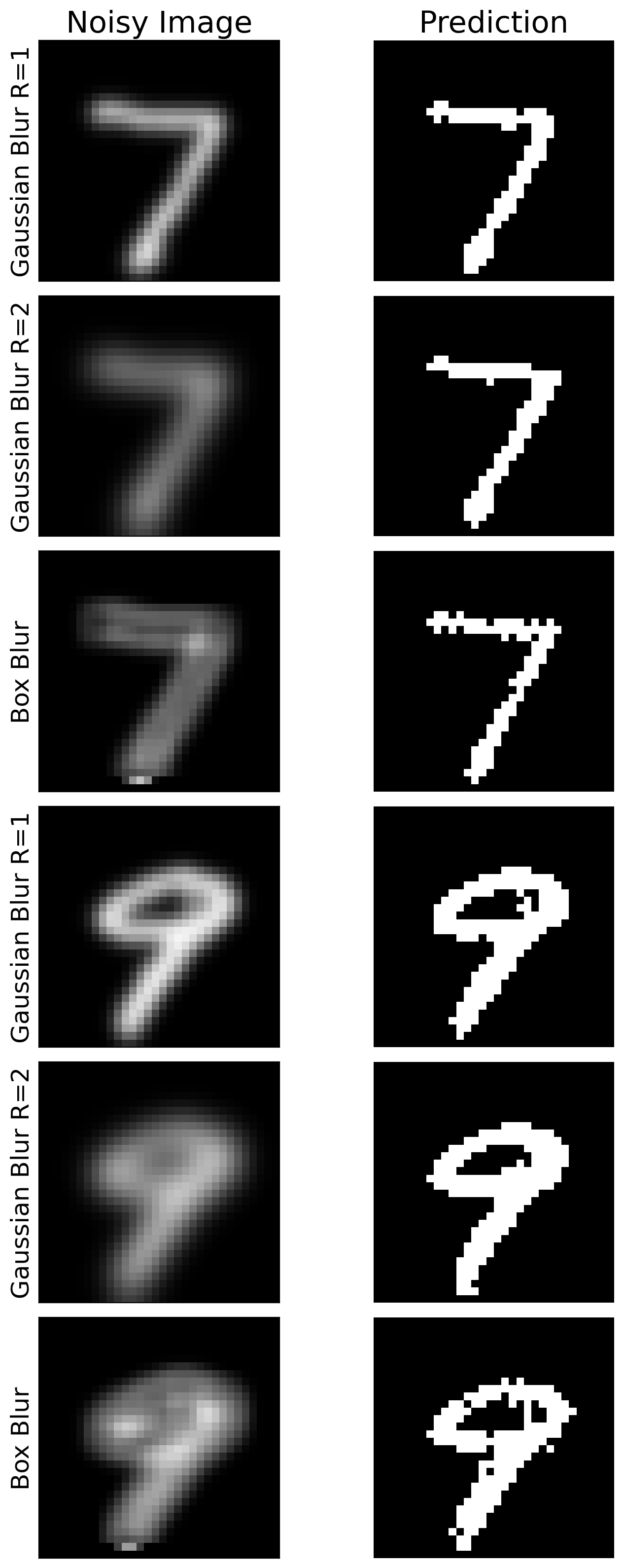
Noisy MNIST. The standard MNIST dataset (Deng 2012) consists of 70,000 grayscale images (50,000 training, 10,000 validation and 10,000 test images). We create three different versions of this dataset for foreground/background segmentation with three noise types respectively: Gaussian blur with radius 1, Gaussian blur with radius 2 and a box blur with a fixed convolutional filter. See Fig. 3 for examples of each noise type.

Results & Discussion

Model	Battery			Noisy MNIST
	IoU	Flops	IoU/GigaFlop	IoU	Flops	IoU/GigaFlop
Matphase (Tabassum et al. 2022)	$0.8144$	$2.11\text{\times}{10}^{12}$	$0.39\text{\times}{10}^{-3}$	—-	—-	—-
DeepLabV3+ (Chen et al. 2018b)	$0.7817$	$1.55\text{\times}{10}^{12}$	$0.51\text{\times}{10}^{-3}$	$0.8459$	$2.07\text{\times}{10}^{13}$	$4.08\text{\times}{10}^{-05}$
SegFormer (Xie et al. 2021)	$0.7692$	$5.84\text{\times}{10}^{11}$	$1.32\text{\times}{10}^{-3}$	$0.8448$	$7.56\text{\times}{10}^{12}$	$1.12\text{\times}{10}^{-4}$
EfficientViT (Cai et al. 2022)	$0.7765$	$4.34\text{\times}{10}^{11}$	$1.79\text{\times}{10}^{-3}$	$0.8344$	$3.72\text{\times}{10}^{14}$	$2.24\text{\times}{10}^{-06}$
IDK-Cascade (Wang et al. 2017)	$0.6987$	$4.20\text{\times}{10}^{11}$	$1.66\text{\times}{10}^{-3}$	$0.7750$	$1.15\text{\times}{10}^{13}$	$6.73\text{\times}{10}^{-05}$
PaSeR-RandPol.	$0.7234$	$5.33\text{\times}{10}^{11}$	$1.36\text{\times}{10}^{-3}$	$0.6376$	$7.05\text{\times}{10}^{12}$	$9.05\text{\times}{10}^{-05}$
PaSeR (ours)	$0.7426$	$1.51\text{\times}{10}^{11}$	$4.91\text{\times}{10}^{-3}$	$0.8231$	$6.51\text{\times}{10}^{12}$	$1.27\text{\times}{10}^{-4}$

Table 1: Battery material phase segmentation and Noisy MNIST results comparison between PaSeR and SOTA models.

Model	Battery			Noisy MNIST
	IoU	Flops	IoU/GigaFlop	IoU	Flops	IoU/GigaFlop
IDK-Cascade (IoU Match)	$0.7444$	$1.54\text{\times}{10}^{12}$	$0.48\text{\times}{10}^{-3}$	$0.7755$	$1.15\text{\times}{10}^{13}$	$6.74\text{\times}{10}^{-05}$
PaSeR (ours)	$0.7426$	$1.51\text{\times}{10}^{11}$	$4.91\text{\times}{10}^{-3}$	$0.8231$	$6.51\text{\times}{10}^{12}$	$1.27\text{\times}{10}^{-4}$

Table 2: Battery material phase segmentation and Noisy MNIST IoU Match Results for PaSeR and IDK-Cascade.

In line with our goal of designing a computationally parsimonious framework, we investigate PaSeR performance in the context of the following research questions.

R1. How does the task performance and computational efficiency of PaSeR compare with the IDK-Cascade paradigm?

R2. How well does PaSeR balance IoU and efficiency relative to SOTA segmentation models?

R3. How adaptable and robust is the PaSeR decision policy to noisy data?

R4. How adaptable and robust is the PaSeR decision policy to task models with complementary strengths?

R5. What are the effects of the various components of PaSeR, ($\lambda$, MC-Sampling) on achieving an effective balance between computational cost and task performance?

R1: Task Performance and Computational Efficiency vs. IDK-Cascade

To evaluate model task performance, we compare our PaSeR model to the cost-aware IDK cascading decision baseline, and a variant of PaSeR (i.e., PaSeR-RandPol.) with the same segmentation models as PaSeR except with a random policy instead of a learned RL policy. The performance results are depicted in Table 1. Looking at the battery dataset, we see that PaSeR outperforms the IDK Cascade model by $\mathbf{6.28}\%$ in terms of the IoU metric. PaSeR also achieves the highest IoU/GigaFlop, outperforming IDK-Cascade by $\mathbf{196}\%$.

Note that the IDK-Cascade model currently under-performs PaSeR on the Battery dataset. Hence, for a fair comparison with our method, we tune the IDK Cascade model to match the IoU performance of PaSeR and denote this model as IDK-Cascade (IoU Match). We achieve this by adjusting the entropy thresholds used in each stage of the cascade until we obtain a least-upper-bound performance (i.e., within a tolerance of $10^{-3}$ of IoU) compared to PaSeR on the same test set. In Table 2, comparing the flops of both models (for the same IoU performance), we see that the PaSeR model requires 90% fewer flops compared to IDK-Cascade (IoU Match) to achieve similar performance. This is further corroborated by the IoU/GigaFlop metric in Table 2 wherein we see that PaSeR achieves a 923% improvement on this metric thereby indicating that PaSeR is able to yield good performance at much lower computational cost compared to the IDK cascading modeling paradigm.

Finally, on the MNIST dataset PaSeR outperforms IDK-Cascade (IoU Match) by $\mathbf{6.1}\%$ and $\mathbf{88.4}\%$ on IoU and IoU/GigaFlop metrics respectively. Here IDK-Cascade (IoU Match) underperforms on the IoU metric vs PaSeR because the entropy based threshold of IDK-Cascade (IoU Match) is not nuanced enough to determine the correct model assignment for a given input. In fact, the accuracy of model assignment by the IDK-Cascade (IoU Match) is only $80\%$ while PaSeR has a model assignment accuracy of $92.7\%$.

R2: Performance Comparison with SOTA Segmentation Models

The problem of battery material phase segmentation has been investigated by a few previous efforts (see Sec. Related Work). The most recent and best model of this group of efforts is MatPhase. We characterize the performance of PaSeR with respect to this SOTA battery material phase segmentation model as well as the recent monolithic SOTA segmentation models DeepLabV3+, SegFormer and EfficientViT. The distributed nature of PaSeR vs monolithic architectures such as SegFormer allows PaSeR to be deployed in an EFC system where monolithic SOTA models would not satisfy computational edge constraints.

In Table 1 we see that although MatPhase  (Tabassum et al. 2022) outperforms PaSeR in terms of segmentation performance, it does so employing significantly more computation. Specifically, MatPhase employs 1297% more computation than PaSeR to obtain a 9.7% performance improvement. Further, we notice that PaSeR achieves a minimum improvement of 174% over all baselines on the IoU/GigaFlop metric. This is a significant result showing the usefulness of PaSeR relative to SOTA models like MatPhase in computationally constrained environments.

When comparing to DeepLabV3+, SegFormer and EfficientViT on the Battery dataset, we see that PaSeR is within $4\%$ of the IoU that those models achieve. Despite their slightly better performance on IoU, PaSeR is much more efficient on the IoU/GigaFlop metric by $\mathbf{863}\%$, $\mathbf{272}\%$ and $\mathbf{174}\%$ for DeepLabV3+, SegFormer and EfficientViT respectively. On the Noisy MNIST dataset, we see the same pattern again. For the DeepLabV3+ model, PaSeR has an $\mathbf{211}\%$ higher IoU/GigaFlop while also outperforming the SegFormer model by $\mathbf{13.4}\%$ on IoU/GigaFlop. The EfficientViT model performs poorly on this dataset because it is designed for high resolution images and downscales the image by a factor of 8 when outputting segmentation maps. To compensate for this downscaling, we upscale our 32x32 MNIST images to 256x256 for this model.

Cityscapes. To demonstrate PaSeR on a modern segmentation task while also integrating pretrained models, we train PaSeR on the Cityscapes dataset (Cordts et al. 2016) using three task models: our small UNet, SegFormer-B0, and SegFormer-B5 with $\lambda=0.10$ achieving a test set IoU of 0.8163 which is comparable with SOTA model performance.

R3: Adaptability to Unseen Contexts (Battery Data)

Figure 3: Examples of types of noise added to MNIST data.

Figure 4: Model assignment confusion matrices for PaSeR, IDK-Cascade and PaSeR-RandPol.

Data and products in real-world (IoT-based) manufacturing pipelines are often plagued by process noise leading to instances from unseen input data distributions. It is in such contexts that the true effectiveness of pipelines such as PaSeR come to the fore in terms of being able to adapt in unseen data contexts.

Model	IoU (Noisy)	Degradation
PaSeR-RandPol.	0.5864	-18.94%
PaSeR	0.7322	-1.4%

Table 3: PaSeR vs PaSeR-RandPol. on noisy datasets. Note that PaSeR-RandPol. fails to adapt in the case of noisy data.

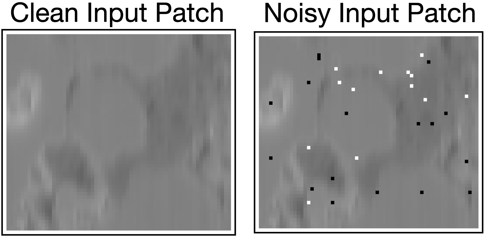
To investigate the adaptability of our RL policy based PaSeR and demonstrate its effectiveness relative to the random policy in PaSeR-RandPol., we create a variant of our battery segmentation dataset injected with salt and pepper noise. This is done to simulate data quality degradation of the input to the segmentation pipeline, due to equipment / process noise. Further, we create pre-trained variants of all segmentation models $\{f_{1},\dots,f_{m}\}$ (except $f_{0}$ i.e., the small U-Net) on a combination of clean and noisy data. Finally, we just replace (without fine-tuning $f_{0}$, $f_{\mathrm{RL}}$) the models $\{f_{1},\dots,f_{m}\}$ in the fully-trained PaSeR model, with variants trained on noisy as well as clean data.

We then investigate performance of PaSeR and PaSeR-RandPol. (both augmented with same set of segmentation models) on a noisy held-out set of data. Note that by leaving $f_{0}$ and RL policy $f_{\mathrm{RL}}$ unaware of the noisy data, we have created a scenario which is unseen w.r.t the RL policy (and model $f_{0}$ on whose predictions and entropy the RL policy decisions are conditioned).

Table 1 showcases IoU segmentation results (on the battery dataset) of PaSeR and PaSeR-RandPol. in the clean data context while Table 3 showcases corresponding IoU results in a noisy context. From these results, we notice that both models experience degradation under the unseen noisy context. However, the degradation in IoU performance experienced by PaSeR is minimal (1.4%), owing to the RL policy being able to adapt, unlike in PaSeR-RandPol. which shows significant performance degradation (18.94%). We find that PaSeR sends 5.7% more patches to the larger models (that have been exposed to the noisy data) than in the clean data case, thereby showcasing strong evidence of adaptability in unseen contexts. This advantage of adaptability in noisy, unseen scenarios with minimal degradation is also a significant advantage of PaSeR and its cost-aware RL model.

R4. Adaptability to Complementary Models (Noisy MNIST)

We demonstrate robustness of PaSeR to utilize models with complementary strengths, on the Noisy MNIST dataset. We train each segmentation model $(f_{0},f_{1},f_{2})$ on the task of foreground/background segmentation on each noisy dataset respectively, training $f_{0}$ on the Gaussian blur with radius 1, $f_{1}$ on Gaussian blur radius 2 and $f_{3}$ on box blur data. Examples of the three noise types are shown in Fig. 3. Each segmentation model learns how to denoise its own noise type and thereby has a unique strength relative to other models.

After training the segmentation models, we train PaSeR’s RL policy with $\lambda=0$ such that it learns the optimal policy without regard for computational cost. We have the dataset containing equal proportions of each noise type, so the optimal policy will send one-third of the images to each segmentation model. Then we fine-tune the pre-trained RL model assuming it has learned an optimal policy. We do this by linearly increasing $\lambda$ while measuring the total variation distance (TVD) from the optimal policy which was previously learned. Once this TVD hits a pre-specified threshold, we stop fine-tuning.

To understand the robustness of the PaSeR RL policy, we examine the model assignment confusion matrices in Fig. 4. Here, PaSeR (with a TVD threshold of 10%) has nearly perfect assignment of images to the $f_{0}$ and $f_{1}$ task models, while only sending 7.2% of images which should have gone to the $f_{2}$ model to the $f_{1}$ model. This occurs because of the 10% TVD threshold, which gives PaSeR the flexibility to send a small percentage of images to the $f_{1}$ model instead of $f_{2}$. Comparing this to the model assignment of IDK-Cascade, we see that it sends 10% of $f_{1}$ model images to $f_{2}$, while also incorrectly sending 7.2% of $f_{2}$ model images to $f_{1}$. This is why IDK-Cascade cannot match the performance of PaSeR. The IDK-Cascade with entropy as the gating mechanism is not adaptable enough to accurately assign images to the best model. Finally, note that the PaSeR-RandPol. assigns images at random to each task model and thereby has the poorest performance across all metrics.

R5: Sensitivity to Hyperparameters

Figure 5: (a) Distribution of entropy estimates with 5 and 20 Monte Carlo Dropout (MCD) samples. (b) PaSeR IoU vs Mean Cost as $\lambda$ changes on battery material phase segmentation dataset.

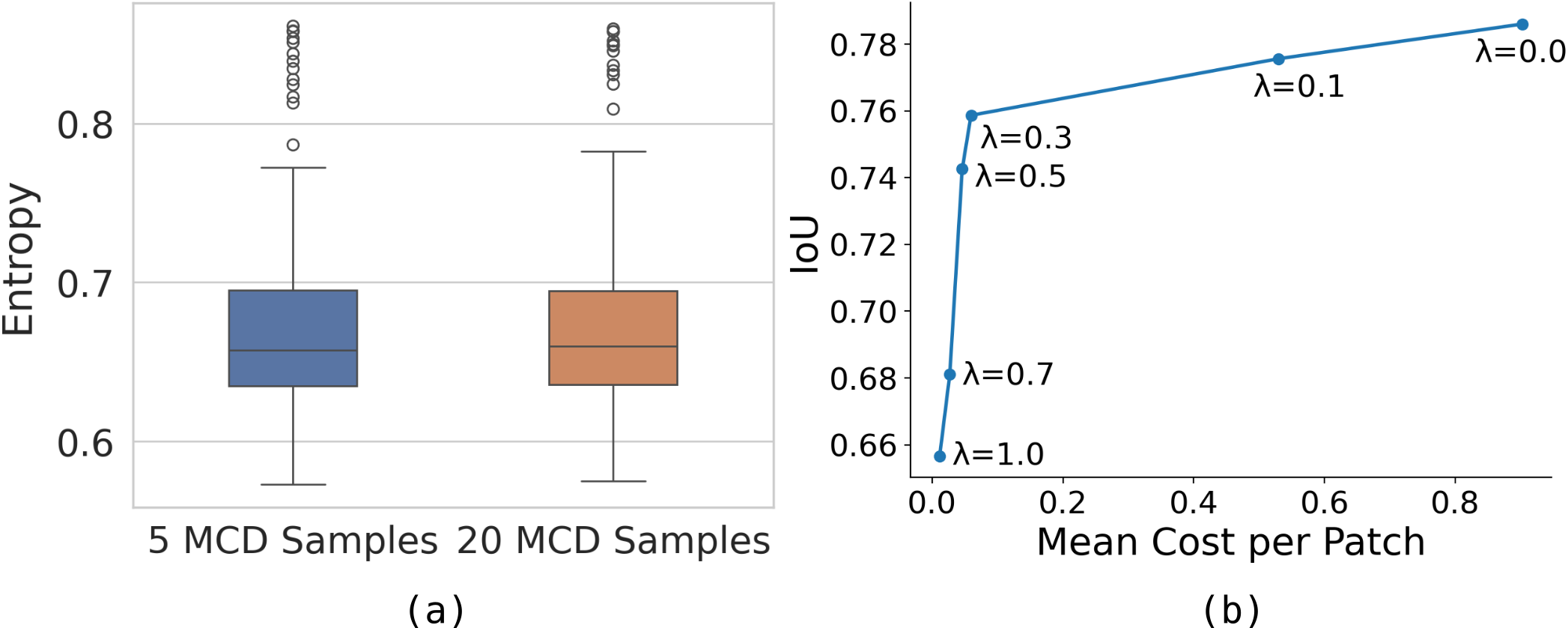
We now investigate how $\lambda$ (cost parameter) and entropy map estimation affect PaSeR performance.

Performance vs Cost Trade-off. In Fig. 5(b), we show PaSeR’s performance/cost trade-off curve as $\lambda$ decreases for the battery segmentation task. The mean cost is calculated using Eq. 3. This cost function is based on the number of parameters in each task model with $f_{2}$ having a significantly higher cost than $f_{1}$. As expected, as $\lambda$ increases, mean cost falls and performance decreases. The sharp drop in cost between $\lambda=0.0$. and $\lambda=0.3$ occurs because of the high difference in the cost of using the large task model $f_{2}$ vs using the smaller models. As $\lambda$ increases in this range, PaSeR uses $f_{2}$ less, leading to a quick drop in mean cost.

Effect of Number of MCDropout Samples. PaSeR computes entropy maps using Monte Carlo (MC) dropout sampling which requires taking multiple samples of each prediction. To test the sensitivity of estimation of entropy to the number of MC samples taken, we show a box plot of the entropy distributions in Fig. 5(a). Comparing 5 MC dropout samples to 20 MC dropout samples shows no significant difference between the distributions of entropies. A t-test between these distributions gives a p-value of 0.6986, allowing us to safely assume these distributions are the same and use 5 MC samples in PaSeR for entropy estimation. We account for these 5 MCD samples in all our previous flops calculations.

Conclusion

In this work, we have developed a computationally parsimonious and more effective alternative to the IDK cascading decision pipeline and demonstrated that our proposed model PaSeR outperforms SOTA models on the task of battery material phase segmentation. We also propose a new metric IoU per GigaFlop which is useful for characterizing effectiveness of models to yield good predictions at low computational cost. Through various qualitative and quantitative results, we demonstrate that PaSeR yields a minimum performance improvement of $\mathbf{174}\%$ on the IoU/GigaFlop metric with respect to compared baselines. We also demonstrate PaSeR’s adaptability to complementary models trained on the noisy MNIST dataset, where it outperforms all baselines on IoU/GigaFlop by a miniumum $\mathbf{13.4}\%$. In the future, we shall extend PaSeR to incorporate other sophisticated cost metrics and test it in the context of multi-model pipelines comprised of data-driven and scientific simulation models.

Appendix A A: Results & Discussion

Figure 6: Side by side comparison of PaSeR segmentation predictions vs corresponding ground truth. We notice that PaSeR yields reliable segmentation results for all classes i.e., pore, nickel, carbon.

Figure 7: Top row (column 1) depicts an example (low-res) input patch that is consistently redirected by the RL policy ($f_{\mathrm{RL}}$) to higher level models while bottom row (column 1) shows a different patch on which predictions by $f_{0}$ are retained and no higher-level predictions are solicited by $f_{\mathrm{RL}}$. Column 4 (last column) depicts corresponding entropy maps output by $f_{0}$ for each patch, while columns 2, 3 depict the predicted segmentation by $f_{0}$ and the corresponding ground truth segmentation. Yellow pixels on each entropy map depict the pixels wherein $f_{0}$ yielded entropy greater than a particular threshold $\gamma$. The top row entropy map has 56% more yellow points than the bottom entropy map indicating significantly higher uncertainty of $f_{0}$ prediction on top image.

A1: Qualitative Battery Segmentation Results

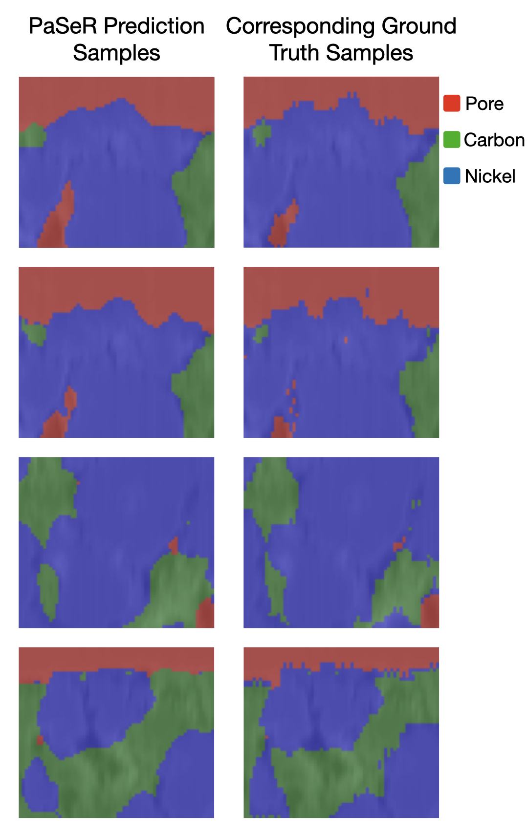
In Fig. 6, we showcase examples of PaSeR segmentation performance on the test set ($\mathcal{D}_{\mathrm{test}}$). We notice that PaSeR yields good segmentation performance even for the challenging (minority) pore, carbon classes as well as the (majority) nickel class.

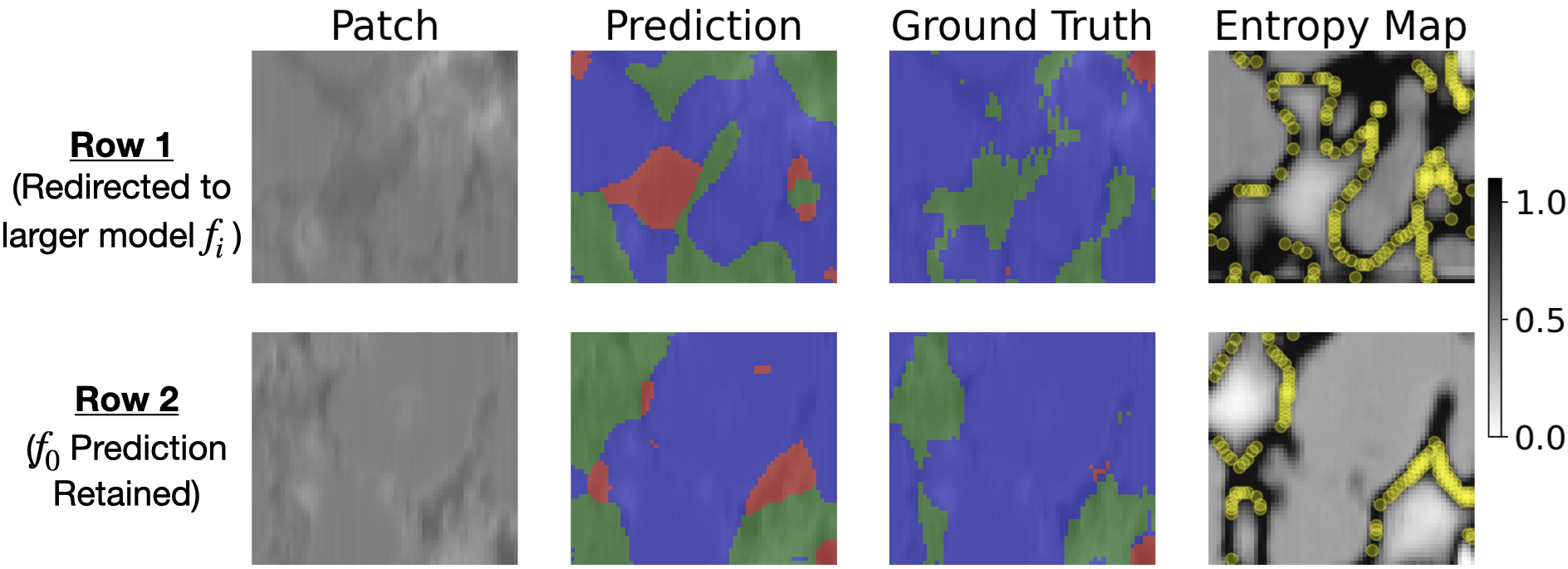
We further investigate the performance of the proposed PaSeR model by investigating how the predictions and entropy maps of $f_{0}$ affect the decisions of $f_{\mathrm{RL}}$. Specifically, we show two separate patches in Fig. 7 such that the patch in the first row is redirected by $f_{\mathrm{RL}}$ to larger models (i.e., in favor of $f_{0}$ predictions) while the $f_{0}$ model predictions are retained by $f_{\mathrm{RL}}$ for the patch in the second row. Although investigating just the low-res input patch (i.e., column 1) of each row, might not yield much insight, the corresponding entropy maps (column 4) showcases that $f_{0}$ predictions on the patch in the first row are significantly less confident as indicated by the presence significantly larger proportion of yellow points which indicate highest entropy regions (i.e., entropy greater than a pre-set threshold $\gamma$) in a much larger portion of the image patch (relative to patch on the bottom row). Specifically, there are 56% more yellow pixels in the top row than the bottom row. The reasoning for such high entropy on the patch in row 1 (relative to row 2) may be gleaned from inspecting the corresponding ground truth images (column 3). We see that the ground truth image in row 1 has significantly more interspersed material phases e.g., the carbon phase - (green) is more interspersed with the nickel (blue) in row 1 than row 2. On the contrary in row 2, the ground truth depicts a more segregated distribution of materials i.e., there exist large contiguous regions of a single material (e.g., large contiguous green, blue regions) which is an easier context for the simpler $f_{0}$ model to segment (owing to its computational simplicity) relative to its more sophisticated counterparts in the PaSeR pipeline. This result further reinforces that PaSeR and the RL policy therein (in conjunction with $f_{0}$) redirect the harder instances (conditioned upon $f_{0}$ predictions, entropy map and governed by the overall computational cost) to upstream models in a computationally parsimonious manner.

Figure 8: Side by side comparison of Noisy MNIST input images and PaSeR predictions.

A2: Qualitative Noisy MNIST Results

In Fig. 8 we show noisy MNIST input samples from our test set in the left column and the corresponding foreground/background PaSeR segmentation predictions in the right column. Note that the box blur images are the most difficult to de-noise, but PaSeR does well on these images because it redirects them to the most sophisticated task model $f_{2}$.

Appendix B B: Experimental Setup

B1: Battery Material Phase Segmentation Data

Our primary dataset consists of 1330 battery phase segmentation tomographic images split into 1270 for training, 20 for validation ($\mathcal{D}_{\mathrm{val}}$), and 40 for testing ($\mathcal{D}_{\mathrm{test}}$). The height and width of each image is 224 x 256. In addition to these images, this dataset contains pixel level annotations of 3 classes: carbon, nickel and pore. We further split the training data into 3 subsets: one for pretraining the segmentation models $\mathcal{D}_{PT}$ with 436 images, another for RL training $\mathcal{D}_{RL}$ with 422 images, and the last for fine-tuning $\mathcal{D}_{FT}$ with 422 images.

Figure 9: Illustration of our patch splitting method with the full image on the left and the patches shown on the right.

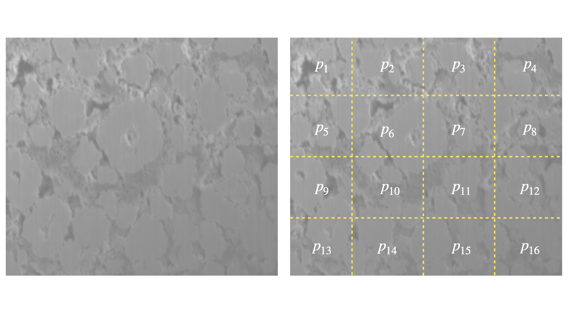
For the input to larger segmentation models $\{f_{1},\ldots,f_{m}\}$, we split the each image into 16 equal size patches, each of size $56\times 64$ as shown in Fig. 9.

Figure 10: To test robustness of PaSeR pipeline in unseen scenarios (e.g., degradation of input images due to process noise), we add noise to our input data and a sample of one such image patch is depicted above.

Figure 11: Each bar indicates the percentage of patches sent to larger (i.e. medium or large) models by PaSeR vs PaSeR-RandPol. when tested on clean (blue) vs (unseen) noisy data (orange). PaSeR sends $\sim 5.7\%$ more patches to larger models in the unseen (noisy) data case, while PaSeR-RandPol. doesn’t adapt and sends the same rate ($\sim 68\%$) of patches to the larger models in both cases.

B1.1: Salt & Pepper Noise

To investigate the adaptability of our RL policy based PaSeR and demonstrate its effectiveness relative to the random policy employed in PaSeR-RandPol., we create a variant of our segmentation dataset injected with salt and pepper noise. This noise was added to every image at a rate of 1% (i.e., noise is injected into 1% of the input pixels). For an example of both clean and noisy images see Fig. 10.

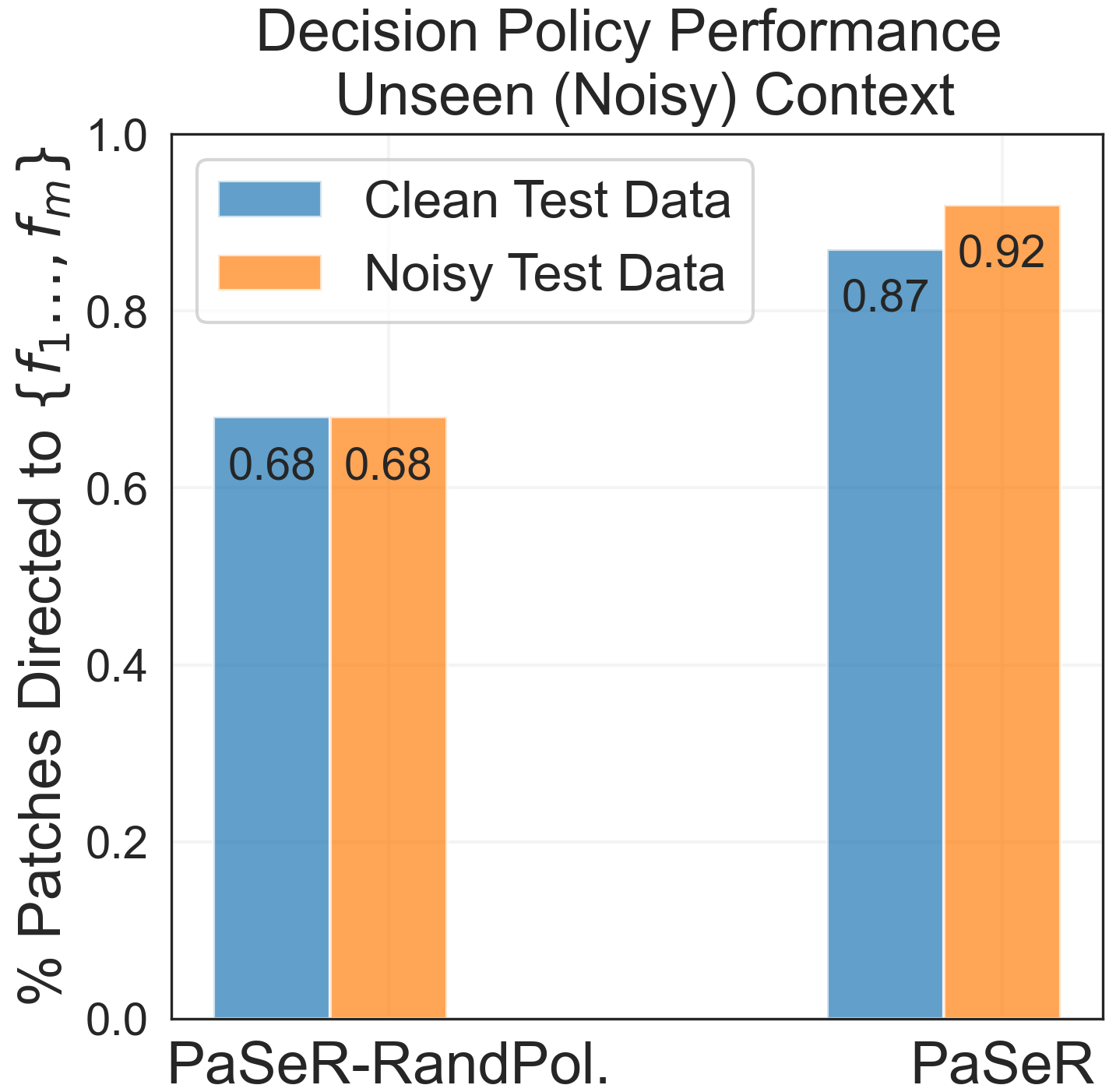
To highlight the response of the RL policy ($f_{\mathrm{RL}}$), when exposed to this unseen noisy scenario during inference, we capture the number of instances redirected to the medium and large models. Specifically, we capture the percentage of patches in which predictions by $f_{0}$ were considered under-confident / under-par by $f_{\mathrm{RL}}$ and instead, predictions from more sophisticated models were sought. In Fig. 11, we showcase this percentage for PaSeR and PaSeR-RandPol. in the clean data (blue) and noisy data (orange) contexts and notice that despite PaSeR RL policy never having encountered noisy data, it is able to recognize that the small model $f_{0}$ is not confident on unseen instances. Hence, in the noisy scenario, it is able to re-direct a higher percentage of patches to more sophisticated upstream models demonstrating robustness of the RL policy learned by PaSeR. In contrast, as PaSeR-RandPol. lacks a learnable policy like PaSeR, it fails to adapt and sends the same percentage of patches to more sophisticated models in clean and noisy scenarios leading to significantly higher performance degradation.

B2: PaSeR for Battery Material Phase Segmentation Hyperparameters and Model Tuning

The PaSeR model requires a few parameters to be specified. Below we describe each parameter as well as the procedure we used to select their values.

Batch Size. We use a batch size of 32 images, which maximizes the usage of the available GPU memory for the large UNet model. For uniformity, we maintain the same batch size for all models during training. However it must be noted that the batch size for each model can be set to different values. During inference or testing, single images (or batches) may be evaluated.

Number of epochs. The 3 stages of our PaSeR model training pipeline: (a) pretraining of segmentation models ($f_{0}$, $f_{1}$, $f_{2}$); (b) training the RL policy ($f_{RL}$); and (c) joint fine-tuning of the segmentation models and RL policy; are executed over the Material Phase Segmentation training datasets (Tabassum et al. 2022) for 200 epochs. This number of epochs was selected as loss convergence was observed (on a validation set) by this time.

Performance-Cost Tradeoff ($\lambda$). As the $\lambda$ parameter is introduced in the form of a convex combination in the RL policy reward, the value of $\lambda$ can be varied in the range [0,1]. We evaluated the effect of $\lambda$ by training the RL policy at values of $\lambda=\{0.0,0.1,0.3,0.5,0.7,0.9,1.0\}$. The $\lambda$ parameter is tuned using grid-search only during the RL pre-training stage (the tuned value is used without further updates during fine-tuning). For our battery phase segmentation experiments, we report IoU and IoU/GigaFlop results with $\lambda=0.5$ because this provides a even balance between task performance and computational cost.

Explore Exploit ($\alpha$). To encourage the RL policy to periodically explore new actions, we tune an explore/exploit parameter $\alpha$ which determines a ratio between the number of times the policy exploits the action yielding the maximum expected return ($s_{f_{RL}}$) and the number of times a random action is chosen ($s_{U}$).

$$s=\begin{cases}s_{f_{RL}}&\text{ with probability }\alpha\\ s_{U}&\text{ with probability }1-\alpha\end{cases}$$ (4)

During RL pretraining, we start the value of $\alpha$ at 0.7 and adopt a linear schedule to increase it (per epoch) until it reaches an upper limit of 0.95. During the fine-tuning stage, we begin $\alpha$ at 0.95 and linearly increase it to 1.0.

Optimizer and Learning Rate $(\eta)$. We use the Adam optimizer (Kingma and Ba 2014) with a learning rate $\eta=1e^{-4}$.

B3: PaSeR for Noisy MNIST Segmentation Hyperparameters and Model Tuning

Figure 12: IoU/GigaFlop vs total variation distance (TVD) after fine-tuning on the noisy MNIST dataset. As we increase the TVD threshold, the IoU/GigaFlop increases because PaSeR sends a greater proportion of images to the smaller models.

We train and run PaSeR on the Noisy MNIST dataset with slightly different parameters than the Battery segmentation dataset in order to demonstrate the adaptability of PaSeR’s RL policy.

Batch Size. We set batch size to 128 because of the relative small size of each instance in this dataset (32 x 32 images).

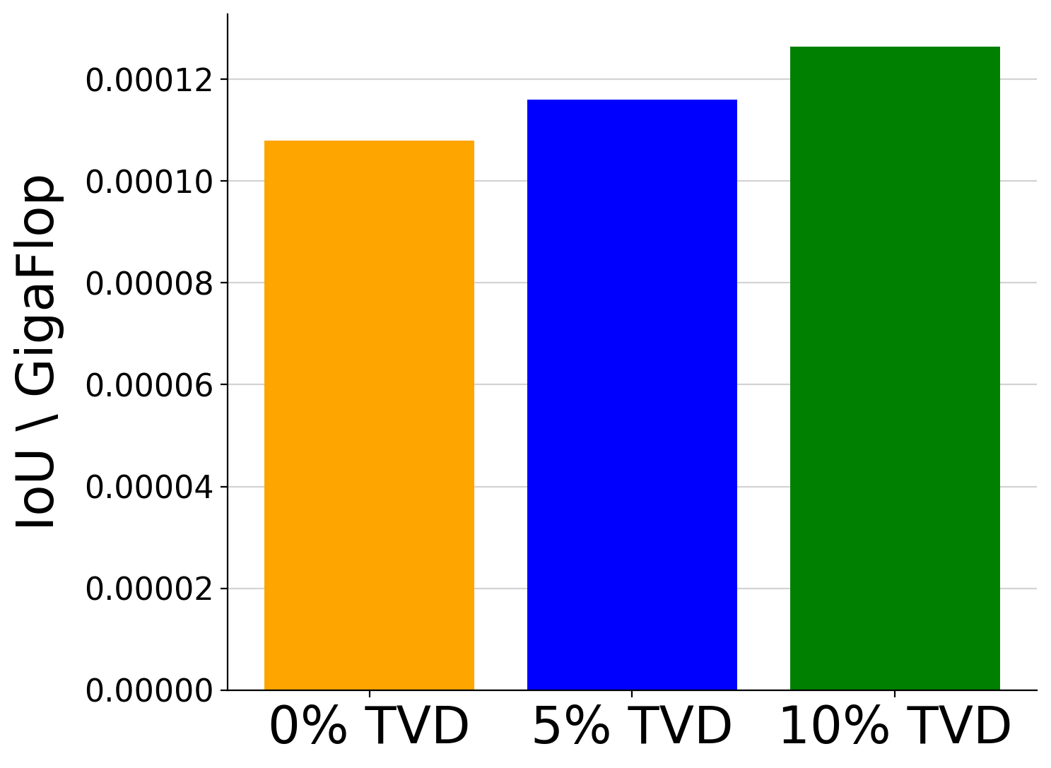
Performance-Cost Tradeoff ($\lambda$). During RL pre-training on this dataset, we set $\lambda=0$ so that the RL policy learned by PaSeR is optimal in terms of IoU without regard for computational cost. Once we have learned this optimal model assignment policy from the data, we set a total variation distance (TVD) percentage threshold from this optimal distribution. During fine-tuning, we increase $\lambda$ on a linear schedule until the newly fine-tuned PaSeR RL policy reaches this TVD threshold, at which point we stop fine-tuning. By increasing $\lambda$, PaSeR is able to trade-off performance for computational cost until the desired deviation from the optimal policy is achieved. In Fig. 12, we plot the effect of increasing TVD thresholds on IoU/GigaFlop efficiency. As expected, increasing the TVD threshold increases the IoU/GigaFlop efficiency of the fine-tuned model. The 0%, 5%, and 10% TVD fine-tuned models have test set IoUs of 0.8432, 0.8328, and 0.8231 respectively.

In real-world applications of PaSeR, the TVD percentage threshold is a straightforward way for domain experts to directly trade-off cost and performance in a dynamic fashion. Consider the case of quality control (QC) for battery manufacturing. In some scenarios, such as small battery manufacturing (AA batteries for example) we would choose a high TVD threshold because the cost of each battery is low and our goal is to quickly and efficiently manufacture them rather than ensure the highest possible quality. However in the case of electric vehicle (EV) batteries, we would set a low TVD threshold because we wish to ensure that the quality of each battery is high and to reduce the chance of early failure or degradation.

B4: IDK-Cascade Hyperparameters and Model Tuning

For the IDK-Cascade model, we setup a cascade with the same three segmentation models as PaSeR (small, medium and large UNets). For each segmentation model $f_{0},f_{1}$, the IDK-Cascade model uses an entropy threshold to decide if a patch should be passed to the next larger model. In addition to these thresholds, we use the same cost function as PaSeR with a cost parameter $\lambda_{IDK}$ weight where $\mathcal{L}(\hat{\mathbf{y}}_{i},\mathbf{y})$ is the cross entropy loss:

$$l_{IDK}=\mathcal{L}(\hat{\mathbf{y}}_{i},\mathbf{y})+\lambda_{IDK}\cdot C(f_{i})$$ (5)

To select the optimal values for entropy thresholds $\alpha_{f_{i}}$, we measure the distribution of entropy values in the validation dataset ($\mathcal{D}_{\mathrm{val}}$) for each model and do a grid search between one standard deviation below and above the mean.

Small UNet Entropy Threshold ($\alpha_{f_{0}}$) For the small UNet entropy threshold, we grid search between $[0.61,0.72]$. This value range was selected as it spanned one standard deviation (above and below) away from the mean entropy computed on the validation set ($\mathcal{D}_{\mathrm{val}}$).

Medium UNet Entropy Threshold ($\alpha_{f_{1}}$) For the medium UNet entropy threshold, we grid search between $[0.20,0.35]$ This value range was selected as it spanned one standard deviation (above and below) away from the mean entropy computed on the validation set ($\mathcal{D}_{\mathrm{val}}$).

Cost weight ($\lambda_{\mathrm{IDK}}$) In (Wang et al. 2017), the authors use $\lambda_{IDK}=0.04$. We follow their example and grid search between $[0.0,1.0]$ and find that $\lambda_{IDK}=0.01$ minimizes the loss in Equation 5

References

- Angelova et al. (2015) Angelova, A.; Krizhevsky, A.; Vanhoucke, V.; Ogale, A.; and Ferguson, D. 2015. Real-Time Pedestrian Detection With Deep Network Cascades. In Proceedings of BMVC 2015.
- Cai et al. (2022) Cai, H.; Li, J.; Hu, M.; Gan, C.; and Han, S. 2022. EfficientViT: Multi-Scale Linear Attention for High-Resolution Dense Prediction. arXiv, 2205.
- Cai, Saberian, and Vasconcelos (2015) Cai, Z.; Saberian, M.; and Vasconcelos, N. 2015. Learning complexity-aware cascades for deep pedestrian detection. In Proceedings of the IEEE international conference on computer vision, 3361–3369.
- Chen et al. (2018a) Chen, B.; Wan, J.; Celesti, A.; Li, D.; Abbas, H.; and Zhang, Q. 2018a. Edge Computing in IoT-Based Manufacturing. IEEE Communications Magazine, 56(9): 103–109.
- Chen et al. (2017) Chen, L.-C.; Papandreou, G.; Schroff, F.; and Adam, H. 2017. Rethinking atrous convolution for semantic image segmentation. arXiv preprint arXiv:1706.05587.
- Chen et al. (2018b) Chen, L.-C.; Zhu, Y.; Papandreou, G.; Schroff, F.; and Adam, H. 2018b. Encoder-decoder with atrous separable convolution for semantic image segmentation. In Proceedings of the European conference on computer vision (ECCV), 801–818.
- Chen et al. (2019) Chen, X.; Williams, B. M.; Vallabhaneni, S. R.; Czanner, G.; Williams, R.; and Zheng, Y. 2019. Learning active contour models for medical image segmentation. In Proceedings of the IEEE/CVF conference on computer vision and pattern recognition, 11632–11640.
- Cordts et al. (2016) Cordts, M.; Omran, M.; Ramos, S.; Rehfeld, T.; Enzweiler, M.; Benenson, R.; Franke, U.; Roth, S.; and Schiele, B. 2016. The cityscapes dataset for semantic urban scene understanding. In Proceedings of the IEEE conference on computer vision and pattern recognition, 3213–3223.
- Deng (2012) Deng, L. 2012. The mnist database of handwritten digit images for machine learning research. IEEE Signal Processing Magazine, 29(6): 141–142.
- Gal and Ghahramani (2016) Gal, Y.; and Ghahramani, Z. 2016. Dropout as a bayesian approximation: Representing model uncertainty in deep learning. In international conference on machine learning, 1050–1059. PMLR.
- Gou et al. (2021) Gou, J.; Yu, B.; Maybank, S. J.; and Tao, D. 2021. Knowledge distillation: A survey. International Journal of Computer Vision, 129: 1789–1819.
- Hinton, Vinyals, and Dean (2015) Hinton, G.; Vinyals, O.; and Dean, J. 2015. Distilling the knowledge in a neural network. arXiv preprint arXiv:1503.02531.
- Hussain et al. (2020) Hussain, F.; Hussain, R.; Hassan, S. A.; and Hossain, E. 2020. Machine learning in IoT security: Current solutions and future challenges. IEEE Communications Surveys & Tutorials, 22(3): 1686–1721.
- Kim et al. (2021) Kim, T.; Oh, J.; Kim, N.; Cho, S.; and Yun, S.-Y. 2021. Comparing kullback-leibler divergence and mean squared error loss in knowledge distillation. arXiv preprint arXiv:2105.08919.
- Kingma and Ba (2014) Kingma, D. P.; and Ba, J. 2014. Adam: A method for stochastic optimization. arXiv preprint arXiv:1412.6980.
- Kirillov et al. (2023) Kirillov, A.; Mintun, E.; Ravi, N.; Mao, H.; Rolland, C.; Gustafson, L.; Xiao, T.; Whitehead, S.; Berg, A. C.; Lo, W.-Y.; et al. 2023. Segment anything. arXiv preprint arXiv:2304.02643.
- Kouris et al. (2022) Kouris, A.; Venieris, S. I.; Laskaridis, S.; and Lane, N. 2022. Multi-exit semantic segmentation networks. In European Conference on Computer Vision, 330–349. Springer.
- Li et al. (2018) Li, H.; Xiong, P.; An, J.; and Wang, L. 2018. Pyramid Attention Network for Semantic Segmentation. arXiv:1805.10180.
- Lu et al. (2020) Lu, X.; Bertei, A.; Finegan, D. P.; Tan, C.; Daemi, S. R.; Weaving, J. S.; O’Regan, K. B.; Heenan, T. M.; Hinds, G.; Kendrick, E.; et al. 2020. 3D microstructure design of lithium-ion battery electrodes assisted by X-ray nano-computed tomography and modelling. Nature communications, 11(1): 2079.
- Meng et al. (2020) Meng, L.; McWilliams, B.; Jarosinski, W.; Park, H.-Y.; Jung, Y.-G.; Lee, J.; and Zhang, J. 2020. Machine learning in additive manufacturing: a review. Jom, 72: 2363–2377.
- Mohammadi et al. (2018) Mohammadi, M.; Al-Fuqaha, A.; Sorour, S.; and Guizani, M. 2018. Deep learning for IoT big data and streaming analytics: A survey. IEEE Communications Surveys & Tutorials, 20(4): 2923–2960.
- Mutlag et al. (2021) Mutlag, A. A.; Abd Ghani, M. K.; Mohammed, M. A.; Lakhan, A.; Mohd, O.; Abdulkareem, K. H.; and Garcia-Zapirain, B. 2021. Multi-agent systems in fog–cloud computing for critical healthcare task management model (CHTM) used for ECG monitoring. Sensors, 21(20): 6923.
- Phuong and Lampert (2019) Phuong, M.; and Lampert, C. 2019. Towards understanding knowledge distillation. In International Conference on Machine Learning, 5142–5151. PMLR.
- Rajapakse, Karunanayake, and Ahmed (2023) Rajapakse, V.; Karunanayake, I.; and Ahmed, N. 2023. Intelligence at the Extreme Edge: A Survey on Reformable TinyML. ACM Computing Surveys.
- Ren, Anicic, and Runkler (2022) Ren, H.; Anicic, D.; and Runkler, T. 2022. How to Manage Tiny Machine Learning at Scale: An Industrial Perspective. arXiv preprint arXiv:2202.09113.
- Ronneberger, Fischer, and Brox (2015) Ronneberger, O.; Fischer, P.; and Brox, T. 2015. U-Net: Convolutional Networks for Biomedical Image Segmentation. arXiv:1505.04597.
- Sutton et al. (1999) Sutton, R. S.; McAllester, D.; Singh, S.; and Mansour, Y. 1999. Policy gradient methods for reinforcement learning with function approximation. Advances in neural information processing systems, 12.
- Tabassum et al. (2022) Tabassum, A.; Muralidhar, N.; Kannan, R.; and Allu, S. 2022. MatPhase: Material phase prediction for Li-ion Battery Reconstruction using Hierarchical Curriculum Learning. In 2022 IEEE International Conference on Big Data (Big Data), 1936–1941. IEEE.
- Tang et al. (2017) Tang, J.; Sun, D.; Liu, S.; and Gaudiot, J.-L. 2017. Enabling deep learning on IoT devices. Computer, 50(10): 92–96.
- Uzkent and Ermon (2020) Uzkent, B.; and Ermon, S. 2020. Learning when and where to zoom with deep reinforcement learning. In Proceedings of the IEEE/CVF conference on computer vision and pattern recognition, 12345–12354.
- Uzkent, Yeh, and Ermon (2020) Uzkent, B.; Yeh, C.; and Ermon, S. 2020. Efficient object detection in large images using deep reinforcement learning. In Proceedings of the IEEE/CVF winter conference on applications of computer vision, 1824–1833.
- Wang et al. (2017) Wang, X.; Luo, Y.; Crankshaw, D.; Tumanov, A.; Yu, F.; and Gonzalez, J. E. 2017. Idk cascades: Fast deep learning by learning not to overthink. arXiv preprint arXiv:1706.00885.
- Xie et al. (2021) Xie, E.; Wang, W.; Yu, Z.; Anandkumar, A.; Alvarez, J. M.; and Luo, P. 2021. SegFormer: Simple and efficient design for semantic segmentation with transformers. Advances in Neural Information Processing Systems, 34: 12077–12090.