Bulk and boundary entanglement transitions in the projective gauge-Higgs model

Abstract

In quantum many-body spin systems, the interplay between the entangling effect of multi-qubit Pauli measurements and the disentangling effect of single-qubit Pauli measurements may give rise to two competing effects. By introducing a randomized measurement pattern with such bases, a phase transition can be induced by altering the ratio between them. In this work, we numerically investigate a measurement-based model associated with the $(2+1)$d $\mathbb{Z}_{2}$ Fradkin-Shenker Hamiltonian model, encompassing the deconfining, confining, and Higgs phases. We determine the phase diagram in our measurement-only model by employing entanglement measures. For the bulk topological order, we use the topological entanglement entropy. We also use the mutual information between separated boundary regions to diagnose the boundary phase transition associated with the Higgs or the bulk SPT phase. We observe the structural similarity between our phase diagram and the one in the standard quantum Hamiltonian formulation of the Fradkin-Shenker model with the open rough boundary. First, a deconfining phase is detected by nonzero and constant topological entanglement entropy. Second, we find a (boundary) phase transition curve separating the Higgs=SPT phase from the rest. In certain limits, the topological phase transitions reside at the critical point of the formation of giant homological cycles in the bulk 3d spacetime lattice, as well as the bond percolation threshold of the boundary 2d spacetime lattice when it is effectively decoupled from the bulk. Additionally, there are analogous mixed-phase properties at a certain region of the phase diagram, emerging from how we terminate the measurement-based procedure. Our findings pave an alternative pathway to study the physics of Higgs=SPT phases on quantum devices in the near future.

I Introduction

Entanglement plays a central role in quantum physics. There are numerous examples of quantum many-body systems that exhibit intricate patterns of entanglement in their ground states. An outstanding example of such entanglement properties is the long-range entanglement (LRE) [1, 2]—also known as the topological order—possessed by Kitaev’s toric code [3], the string-net models [4], and so on. In the absence of LRE, a state is said to have short-range entanglement (SRE). Such a state may have a nontrivial entanglement pattern if one imposes global symmetries, giving rise to the notion of symmetry-protected topological (SPT) order [5, 6, 7, 8, 9, 10, 11, 12]. Classification of entanglement in the low-energy regime of quantum many-body systems has been one of the major subjects in condensed matter physics over a decade [13].

In recent years, there has been growing interest in the study of phase transitions in entanglement under evolution involving both unitary operators and non-unitary operators such as measurements [14, 15, 16, 17]. The interplay between multi-qubit entangling unitary gates and single-qubit measurements exhibits competing effects on entanglement and can lead to phase transitions when the rate of projective measurement is varied, which is known as measurement-induced phase transitions (MIPT) [18, 19, 20, 21, 22]. Some studies have focused on special classes of unitary gates, such as the Clifford gates or Majorana fermions, which can be efficiently simulated classically in combination with Pauli measurements due to the Gottesman-Knill theorem [18, 19, 20, 23, 24, 25, 26, 27, 28, 29, 30, 31, 32, 33, 34, 35, 36, 37, 38, 39]. These investigations have provided insights into the critical behavior of MIPT with fairly large system sizes. Other works have mapped MIPT circuits, including both Clifford and random (Haar) unitary circuits, to classical statistical models, such as the percolation model [40, 28, 29, 41, 42, 34, 35, 43, 44, 39, 45, 38], which describe the underlying entanglement structure in spacetime.

Interestingly, the competition between entangling and disentangling effects can arise not only from unitary gates and measurements. In fact, phase transitions can also be induced by non-commuting single-qubit measurements and multi-qubit measurements [46, 47, 48, 49, 50, 32, 33, 41, 35, 51, 52, 53, 54, 55], even in the absence of independent unitary gates. This scenario is termed as a measurement-only (MO) circuit (MOC) or a projective model in the literature. For instance, Lang and Büchler explored a model called the projective transverse-field Ising (pTFI) model in Ref. [47]. In this model, the projective measurement bases consist of the single-qubit $X$ basis and the two-qubit $ZZ$ basis for adjacent sites. Each quantum trajectory of the state evolves according to a randomized measurement pattern with these bases, and the entanglement measure, such as the von Neumann entropy, is computed for each trajectory, followed by an average over samples of randomized measurement patterns. The averaged entanglement measure reaches an equilibrium (with respect to time steps), and the measurement ratio determines whether the state is in the trivial order or in the GHZ order on average. The pTFI model has been extended to several other setups [48, 49, 30, 51, 53, 50, 52]. In this work, we investigate yet another MOC model related to a lattice gauge model with interesting phases and perform numerical simulations to determine relevant physical properties.

From a broader perspective, MOC models may be seen as specialized models of Measurement-Based Quantum Computation (MBQC) [56, 57, 58, 59, 60]. Indeed, Nielsen showed that the universal quantum computation can be achieved by single- and multi-qubit measurements alone [61] (see also the review [60]). We remark that MOC models utilize measurements with the Pauli or Pauli product basis, and as such, they do not require adaptive determination of parameters for measurement bases unlike in the universal MBQC. The perspective from MBQC, although not our main focus, will be used at some point in our paper.

In parallel to the development in MIPT, the Higgs phase of gauge theory with matter has gained interest from the viewpoint of the landscape of quantum phases. The phase diagram of the gauge-Higgs model contains the confining, deconfining, and Higgs phases [62, 63]. For the model without boundaries, Fradkin and Shenker showed that there is no clear transition between Higgs and confining phases; the two are analytically connected. If we consider the model with certain types of boundaries, however, the Fradkin-Shenker model was recently shown to experience a phase transition [64]. The model hosts degenerate modes on the boundary of the lattice when the model parameters are so that the open Wilson line operator, whose endpoints are attached with charges, has non-vanishing values in the bulk. The Higgs phase of the gauge theory is now interpreted as an SPT phase protected by matter and magnetic symmetries [64]. In this work, a crucial question we ask is whether such a structure of phase transitions can also occur in an MIPT/MOC setup.

The setup of our investigation is an MO circuit whose measurement bases mimic the Hamiltonian terms in the $(2+1)$d Fradkin-Shenker model on a 2d lattice with a boundary. We obtain a phase diagram, parameterized by two measurement ratios, that contains three phases as the Hamiltonian model—the topological order (deconfining phase), the SPT order (Higgs phase), and the trivial order (confining phase). As a diagnostic of the topological order in the MOC, we compute the topological entanglement entropy [65, 66] in the bulk and show that there is a region with constant topological entanglement and a clear phase transition separating this region from the rest. As a diagnostic of the SPT order, on the other hand, we will essentially diagnose a GHZ state induced at the boundary of the lattice. To do so, we compute the mutual information between a pair of boundary regions; our idea traces back to the original study by Lang and Büchler, who studied the phase transition in 1d pTFI model by a mutual information [47]. Our numerical result shows a strikingly clear phase boundary separating the Higgs phase from the rest, which is in agreement with the recent proposition of ‘Higgs=SPT’ [64] in the Hamiltonian picture. The above two phases are robust entanglement properties of our MO circuit in the sense that they are both robustly detected regardless of how we terminate our measurement rounds, as long as there are sufficient number of them. Interestingly, we will also show that our MO circuit hosts a mixed phase, which is characterized by alternating appearance of the cluster state and the product state in the bulk (at one specific corner of the phase diagram), depending on how we end our circuit. This will be detected by a non-local bulk quantity. Remarkably, this observable exhibits continuity between the Higgs limit and the confining limit, whereas it also shows a clear separation from the deconfining phase—a picture consistent with the original proposition by Fradkin and Shenker.

Our study is somewhat similar to a recent work [67] done by Kuno, Orito, and Ichinose, who studied an MOC inspired by the dual of the Fradkin-Shenker model. We note that our setup, however, has several differences, and we probe different aspects. We shall illuminate various new connections to the physics of Higgs=SPT, as well as underlying mathematical structures in this paper.

This paper is organized as follows. In Section II, we present our results on a study of the Fradkin-Shenker MOC model. We first define our setup and then discuss the diagnostics of quantum orders in our MOC. We provide our numerical results and present our interpretation in terms of percolation. Section III is devoted to conclusions and discussion.

II Projective-gauge-Higgs MOC

II.1 Setup of the circuit

Let $X$ and $Z$ be the Pauli $X$ and $Z$ operators, respectively. We denote their eigenvectors as

$$Z|0\rangle=|0\rangle,\quad Z|1\rangle=-|1\rangle,$$ (1)

$$X|+\rangle=|+\rangle,\quad X|-\rangle=-|-\rangle,$$ (2)

$$|+\rangle=\frac{|0\rangle+|1\rangle}{\sqrt{2}},\quad|-\rangle=\frac{|0\rangle-|1\rangle}{\sqrt{2}}.$$ (3)

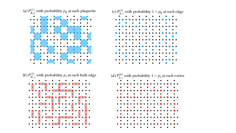
The Hilbert space is defined as the tensor product of qubits placed on vertices $V$ and edges $E$ of the 2d square lattice; this is also called the Lieb lattice. We consider primarily the Lieb lattice with the so-called rough boundary so that the boundary of the lattice consists of edges perpendicular to it. (We have also considered the smooth boundary condition but remark that the rough boundary allows us to better detect the transition via mutual information. The choice of the rough boundary was motivated by the setup in the work ‘Higgs=SPT’ by Verresen and collaborators [64].) We have three types of cells: plaquettes $P$, edges $E$, and vertices $V$. When clarification is needed, we use subscripts $B$ and $\partial$ to indicate the set of cells is restricted to the bulk and the boundary, respectively. For instance, $E_{B}$ denotes the set of all edges in the bulk, $E_{\partial}$ denotes the set of all edges on the boundary, $E_{B\partial}$ denotes the set of all of those in the bulk or on the boundary, and so on. See Fig. 1 for illustration of our setup.

To define our measurement bases, we write

$$W_{e} =Z_{e}\prod_{v\subset e}Z_{v}=\raisebox{-10.0pt}{ \leavevmode\hbox to52.21pt{\vbox to23.76pt{\pgfpicture\makeatletter\hbox{\hskip 11.88092pt\lower-11.88092pt\hbox to0.0pt{\pgfsys@beginscope\pgfsys@invoke{ }\definecolor{pgfstrokecolor}{rgb}{0,0,0}\pgfsys@color@rgb@stroke{0}{0}{0}\pgfsys@invoke{ }\pgfsys@color@rgb@fill{0}{0}{0}\pgfsys@invoke{ }\pgfsys@setlinewidth{0.4pt}\pgfsys@invoke{ }\nullfont\pgfsys@beginscope\pgfsys@invoke{ }\pgfsys@invoke{\lxSVG@closescope }\pgfsys@endscope\hbox to0.0pt{\pgfsys@beginscope\pgfsys@invoke{ }{}{{}}{} {}{}\pgfsys@beginscope\pgfsys@invoke{ }\color[rgb]{0.7,0.7,0.7}\definecolor[named]{pgfstrokecolor}{rgb}{0.7,0.7,0.7}\pgfsys@color@gray@stroke{0.7}\pgfsys@invoke{ }\pgfsys@color@gray@fill{0.7}\pgfsys@invoke{ }\definecolor{pgffillcolor}{rgb}{0.7,0.7,0.7}\pgfsys@setlinewidth{1.0pt}\pgfsys@invoke{ }{}\pgfsys@moveto{-11.38092pt}{0.0pt}\pgfsys@lineto{39.83368pt}{0.0pt}\pgfsys@stroke\pgfsys@invoke{ } \pgfsys@invoke{\lxSVG@closescope }\pgfsys@endscope{}{{}}{} {}{}\pgfsys@beginscope\pgfsys@invoke{ }\color[rgb]{0.7,0.7,0.7}\definecolor[named]{pgfstrokecolor}{rgb}{0.7,0.7,0.7}\pgfsys@color@gray@stroke{0.7}\pgfsys@invoke{ }\pgfsys@color@gray@fill{0.7}\pgfsys@invoke{ }\definecolor{pgffillcolor}{rgb}{0.7,0.7,0.7}\pgfsys@setlinewidth{1.0pt}\pgfsys@invoke{ }{}\pgfsys@moveto{0.0pt}{-11.38092pt}\pgfsys@lineto{0.0pt}{11.38092pt}\pgfsys@stroke\pgfsys@invoke{ } \pgfsys@invoke{\lxSVG@closescope }\pgfsys@endscope{}{{}}{} {}{}\pgfsys@beginscope\pgfsys@invoke{ }\color[rgb]{0.7,0.7,0.7}\definecolor[named]{pgfstrokecolor}{rgb}{0.7,0.7,0.7}\pgfsys@color@gray@stroke{0.7}\pgfsys@invoke{ }\pgfsys@color@gray@fill{0.7}\pgfsys@invoke{ }\definecolor{pgffillcolor}{rgb}{0.7,0.7,0.7}\pgfsys@setlinewidth{1.0pt}\pgfsys@invoke{ }{}\pgfsys@moveto{28.45276pt}{-11.38092pt}\pgfsys@lineto{28.45276pt}{11.38092pt}\pgfsys@stroke\pgfsys@invoke{ } \pgfsys@invoke{\lxSVG@closescope }\pgfsys@endscope{{}}\hbox{\hbox{{\pgfsys@beginscope\pgfsys@invoke{ }{{}{}{{ {}{}}}{ {}{}} {{}{{}}}{{}{}}{}{{}{}} { }{{{{}}\pgfsys@beginscope\pgfsys@invoke{ }\pgfsys@transformcm{1.0}{0.0}{0.0}{1.0}{24.68193pt}{-3.41666pt}\pgfsys@invoke{ }\hbox{{\definecolor{pgfstrokecolor}{rgb}{0,0,0}\pgfsys@color@rgb@stroke{0}{0}{0}\pgfsys@invoke{ }\pgfsys@color@rgb@fill{0}{0}{0}\pgfsys@invoke{ }\hbox{{$Z$}} }}\pgfsys@invoke{\lxSVG@closescope }\pgfsys@endscope}}} \pgfsys@invoke{\lxSVG@closescope }\pgfsys@endscope}}} {{}}\hbox{\hbox{{\pgfsys@beginscope\pgfsys@invoke{ }{{}{}{{ {}{}}}{ {}{}} {{}{{}}}{{}{}}{}{{}{}} { }{{{{}}\pgfsys@beginscope\pgfsys@invoke{ }\pgfsys@transformcm{1.0}{0.0}{0.0}{1.0}{10.45555pt}{-3.41666pt}\pgfsys@invoke{ }\hbox{{\definecolor{pgfstrokecolor}{rgb}{0,0,0}\pgfsys@color@rgb@stroke{0}{0}{0}\pgfsys@invoke{ }\pgfsys@color@rgb@fill{0}{0}{0}\pgfsys@invoke{ }\hbox{{$Z$}} }}\pgfsys@invoke{\lxSVG@closescope }\pgfsys@endscope}}} \pgfsys@invoke{\lxSVG@closescope }\pgfsys@endscope}}} {{}}\hbox{\hbox{{\pgfsys@beginscope\pgfsys@invoke{ }{{}{}{{ {}{}}}{ {}{}} {{}{{}}}{{}{}}{}{{}{}} { }{{{{}}\pgfsys@beginscope\pgfsys@invoke{ }\pgfsys@transformcm{1.0}{0.0}{0.0}{1.0}{-3.77083pt}{-3.41666pt}\pgfsys@invoke{ }\hbox{{\definecolor{pgfstrokecolor}{rgb}{0,0,0}\pgfsys@color@rgb@stroke{0}{0}{0}\pgfsys@invoke{ }\pgfsys@color@rgb@fill{0}{0}{0}\pgfsys@invoke{ }\hbox{{$Z$}} }}\pgfsys@invoke{\lxSVG@closescope }\pgfsys@endscope}}} \pgfsys@invoke{\lxSVG@closescope }\pgfsys@endscope}}} \pgfsys@invoke{\lxSVG@closescope }\pgfsys@endscope{}{}{}\hss}\pgfsys@discardpath\pgfsys@invoke{\lxSVG@closescope }\pgfsys@endscope\hss}}\lxSVG@closescope\endpgfpicture}} }\quad\forall e\in E_{B}, Z Z Z Z Z Z$$ (4)

$$B_{p} =\prod_{e\subset p}Z_{e}=\raisebox{-20.0pt}{ \leavevmode\hbox to42.66pt{\vbox to41.38pt{\pgfpicture\makeatletter\hbox{\hskip 21.33022pt\lower-19.55331pt\hbox to0.0pt{\pgfsys@beginscope\pgfsys@invoke{ }\definecolor{pgfstrokecolor}{rgb}{0,0,0}\pgfsys@color@rgb@stroke{0}{0}{0}\pgfsys@invoke{ }\pgfsys@color@rgb@fill{0}{0}{0}\pgfsys@invoke{ }\pgfsys@setlinewidth{0.4pt}\pgfsys@invoke{ }\nullfont\pgfsys@beginscope\pgfsys@invoke{ }\pgfsys@invoke{\lxSVG@closescope }\pgfsys@endscope\hbox to0.0pt{\pgfsys@beginscope\pgfsys@invoke{ }{}{{}}{} {}{} {}{} {}{} {}{}\pgfsys@beginscope\pgfsys@invoke{ }\color[rgb]{0.7,0.7,0.7}\definecolor[named]{pgfstrokecolor}{rgb}{0.7,0.7,0.7}\pgfsys@color@gray@stroke{0.7}\pgfsys@invoke{ }\pgfsys@color@gray@fill{0.7}\pgfsys@invoke{ }\definecolor{pgffillcolor}{rgb}{0.7,0.7,0.7}\pgfsys@setlinewidth{1.0pt}\pgfsys@invoke{ }{}\pgfsys@moveto{-14.22638pt}{-14.22638pt}\pgfsys@lineto{14.22638pt}{-14.22638pt}\pgfsys@lineto{14.22638pt}{14.22638pt}\pgfsys@lineto{-14.22638pt}{14.22638pt}\pgfsys@lineto{-14.22638pt}{-14.22638pt}\pgfsys@stroke\pgfsys@invoke{ } \pgfsys@invoke{\lxSVG@closescope }\pgfsys@endscope{{}}\hbox{\hbox{{\pgfsys@beginscope\pgfsys@invoke{ }{{}{}{{ {}{}}}{ {}{}} {{}{{}}}{{}{}}{}{{}{}} { }{{{{}}\pgfsys@beginscope\pgfsys@invoke{ }\pgfsys@transformcm{1.0}{0.0}{0.0}{1.0}{-17.99721pt}{-1.99394pt}\pgfsys@invoke{ }\hbox{{\definecolor{pgfstrokecolor}{rgb}{0,0,0}\pgfsys@color@rgb@stroke{0}{0}{0}\pgfsys@invoke{ }\pgfsys@color@rgb@fill{0}{0}{0}\pgfsys@invoke{ }\hbox{{$Z$}} }}\pgfsys@invoke{\lxSVG@closescope }\pgfsys@endscope}}} \pgfsys@invoke{\lxSVG@closescope }\pgfsys@endscope}}} {{}}\hbox{\hbox{{\pgfsys@beginscope\pgfsys@invoke{ }{{}{}{{ {}{}}}{ {}{}} {{}{{}}}{{}{}}{}{{}{}} { }{{{{}}\pgfsys@beginscope\pgfsys@invoke{ }\pgfsys@transformcm{1.0}{0.0}{0.0}{1.0}{10.45555pt}{-1.99394pt}\pgfsys@invoke{ }\hbox{{\definecolor{pgfstrokecolor}{rgb}{0,0,0}\pgfsys@color@rgb@stroke{0}{0}{0}\pgfsys@invoke{ }\pgfsys@color@rgb@fill{0}{0}{0}\pgfsys@invoke{ }\hbox{{$Z$}} }}\pgfsys@invoke{\lxSVG@closescope }\pgfsys@endscope}}} \pgfsys@invoke{\lxSVG@closescope }\pgfsys@endscope}}} {{}}\hbox{\hbox{{\pgfsys@beginscope\pgfsys@invoke{ }{{}{}{{ {}{}}}{ {}{}} {{}{{}}}{{}{}}{}{{}{}} { }{{{{}}\pgfsys@beginscope\pgfsys@invoke{ }\pgfsys@transformcm{1.0}{0.0}{0.0}{1.0}{-3.77083pt}{11.66327pt}\pgfsys@invoke{ }\hbox{{\definecolor{pgfstrokecolor}{rgb}{0,0,0}\pgfsys@color@rgb@stroke{0}{0}{0}\pgfsys@invoke{ }\pgfsys@color@rgb@fill{0}{0}{0}\pgfsys@invoke{ }\hbox{{$Z$}} }}\pgfsys@invoke{\lxSVG@closescope }\pgfsys@endscope}}} \pgfsys@invoke{\lxSVG@closescope }\pgfsys@endscope}}} {{}}\hbox{\hbox{{\pgfsys@beginscope\pgfsys@invoke{ }{{}{}{{ {}{}}}{ {}{}} {{}{{}}}{{}{}}{}{{}{}} { }{{{{}}\pgfsys@beginscope\pgfsys@invoke{ }\pgfsys@transformcm{1.0}{0.0}{0.0}{1.0}{-3.77083pt}{-16.2203pt}\pgfsys@invoke{ }\hbox{{\definecolor{pgfstrokecolor}{rgb}{0,0,0}\pgfsys@color@rgb@stroke{0}{0}{0}\pgfsys@invoke{ }\pgfsys@color@rgb@fill{0}{0}{0}\pgfsys@invoke{ }\hbox{{$Z$}} }}\pgfsys@invoke{\lxSVG@closescope }\pgfsys@endscope}}} \pgfsys@invoke{\lxSVG@closescope }\pgfsys@endscope}}} \pgfsys@invoke{\lxSVG@closescope }\pgfsys@endscope{}{}{}\hss}\pgfsys@discardpath\pgfsys@invoke{\lxSVG@closescope }\pgfsys@endscope\hss}}\lxSVG@closescope\endpgfpicture}} }\quad\forall p\in P_{B}. Z Z Z Z Z Z Z Z$$ (5)

The term $W_{e}$ describes a coupling among the gauge degrees of freedom on an edge and the two matter degrees of freedom on the vertices adjacent to it. Note that we do not introduce such a term to measure for edges on the rough boundary, as each of them only contains a single vertex. On the other hand, the term $B_{p}$ is the plaquette term, which describes the magnetic interaction in the gauge theory. The plaquette term in the bulk is the product over the four gauge degrees of freedom around a plaquette. On the rough boundary, we define it as the product over three gauge degrees of freedom. At the four corners of the lattice, we define it as the product over the two edges that sit at the corner. We also write the Gauss law divergence operator as

$$G_{v}=X_{v}\prod_{e\supset v}X_{e}=\raisebox{-18.0pt}{ \leavevmode\hbox to44.19pt{\vbox to41.95pt{\pgfpicture\makeatletter\hbox{\hskip 7.86772pt\lower-20.97604pt\hbox to0.0pt{\pgfsys@beginscope\pgfsys@invoke{ }\definecolor{pgfstrokecolor}{rgb}{0,0,0}\pgfsys@color@rgb@stroke{0}{0}{0}\pgfsys@invoke{ }\pgfsys@color@rgb@fill{0}{0}{0}\pgfsys@invoke{ }\pgfsys@setlinewidth{0.4pt}\pgfsys@invoke{ }\nullfont\pgfsys@beginscope\pgfsys@invoke{ }\pgfsys@invoke{\lxSVG@closescope }\pgfsys@endscope\hbox to0.0pt{\pgfsys@beginscope\pgfsys@invoke{ }{}{{}}{} {}{}\pgfsys@beginscope\pgfsys@invoke{ }\color[rgb]{0.7,0.7,0.7}\definecolor[named]{pgfstrokecolor}{rgb}{0.7,0.7,0.7}\pgfsys@color@gray@stroke{0.7}\pgfsys@invoke{ }\pgfsys@color@gray@fill{0.7}\pgfsys@invoke{ }\definecolor{pgffillcolor}{rgb}{0.7,0.7,0.7}\pgfsys@setlinewidth{1.0pt}\pgfsys@invoke{ }{}\pgfsys@moveto{0.0pt}{0.0pt}\pgfsys@lineto{28.45276pt}{0.0pt}\pgfsys@stroke\pgfsys@invoke{ } \pgfsys@invoke{\lxSVG@closescope }\pgfsys@endscope{}{{}}{} {}{}\pgfsys@beginscope\pgfsys@invoke{ }\color[rgb]{0.7,0.7,0.7}\definecolor[named]{pgfstrokecolor}{rgb}{0.7,0.7,0.7}\pgfsys@color@gray@stroke{0.7}\pgfsys@invoke{ }\pgfsys@color@gray@fill{0.7}\pgfsys@invoke{ }\definecolor{pgffillcolor}{rgb}{0.7,0.7,0.7}\pgfsys@setlinewidth{1.0pt}\pgfsys@invoke{ }{}\pgfsys@moveto{14.22638pt}{-14.22638pt}\pgfsys@lineto{14.22638pt}{14.22638pt}\pgfsys@stroke\pgfsys@invoke{ } \pgfsys@invoke{\lxSVG@closescope }\pgfsys@endscope{{}}\hbox{\hbox{{\pgfsys@beginscope\pgfsys@invoke{ }{{}{}{{ {}{}}}{ {}{}} {{}{{}}}{{}{}}{}{{}{}} { }{{{{}}\pgfsys@beginscope\pgfsys@invoke{ }\pgfsys@transformcm{1.0}{0.0}{0.0}{1.0}{-4.53471pt}{-3.41666pt}\pgfsys@invoke{ }\hbox{{\definecolor{pgfstrokecolor}{rgb}{0,0,0}\pgfsys@color@rgb@stroke{0}{0}{0}\pgfsys@invoke{ }\pgfsys@color@rgb@fill{0}{0}{0}\pgfsys@invoke{ }\hbox{{$X$}} }}\pgfsys@invoke{\lxSVG@closescope }\pgfsys@endscope}}} \pgfsys@invoke{\lxSVG@closescope }\pgfsys@endscope}}} {{}}\hbox{\hbox{{\pgfsys@beginscope\pgfsys@invoke{ }{{}{}{{ {}{}}}{ {}{}} {{}{{}}}{{}{}}{}{{}{}} { }{{{{}}\pgfsys@beginscope\pgfsys@invoke{ }\pgfsys@transformcm{1.0}{0.0}{0.0}{1.0}{9.69167pt}{-3.41666pt}\pgfsys@invoke{ }\hbox{{\definecolor{pgfstrokecolor}{rgb}{0,0,0}\pgfsys@color@rgb@stroke{0}{0}{0}\pgfsys@invoke{ }\pgfsys@color@rgb@fill{0}{0}{0}\pgfsys@invoke{ }\hbox{{$X$}} }}\pgfsys@invoke{\lxSVG@closescope }\pgfsys@endscope}}} \pgfsys@invoke{\lxSVG@closescope }\pgfsys@endscope}}} {{}}\hbox{\hbox{{\pgfsys@beginscope\pgfsys@invoke{ }{{}{}{{ {}{}}}{ {}{}} {{}{{}}}{{}{}}{}{{}{}} { }{{{{}}\pgfsys@beginscope\pgfsys@invoke{ }\pgfsys@transformcm{1.0}{0.0}{0.0}{1.0}{23.91805pt}{-3.41666pt}\pgfsys@invoke{ }\hbox{{\definecolor{pgfstrokecolor}{rgb}{0,0,0}\pgfsys@color@rgb@stroke{0}{0}{0}\pgfsys@invoke{ }\pgfsys@color@rgb@fill{0}{0}{0}\pgfsys@invoke{ }\hbox{{$X$}} }}\pgfsys@invoke{\lxSVG@closescope }\pgfsys@endscope}}} \pgfsys@invoke{\lxSVG@closescope }\pgfsys@endscope}}} {{}}\hbox{\hbox{{\pgfsys@beginscope\pgfsys@invoke{ }{{}{}{{ {}{}}}{ {}{}} {{}{{}}}{{}{}}{}{{}{}} { }{{{{}}\pgfsys@beginscope\pgfsys@invoke{ }\pgfsys@transformcm{1.0}{0.0}{0.0}{1.0}{9.69167pt}{10.80972pt}\pgfsys@invoke{ }\hbox{{\definecolor{pgfstrokecolor}{rgb}{0,0,0}\pgfsys@color@rgb@stroke{0}{0}{0}\pgfsys@invoke{ }\pgfsys@color@rgb@fill{0}{0}{0}\pgfsys@invoke{ }\hbox{{$X$}} }}\pgfsys@invoke{\lxSVG@closescope }\pgfsys@endscope}}} \pgfsys@invoke{\lxSVG@closescope }\pgfsys@endscope}}} {{}}\hbox{\hbox{{\pgfsys@beginscope\pgfsys@invoke{ }{{}{}{{ {}{}}}{ {}{}} {{}{{}}}{{}{}}{}{{}{}} { }{{{{}}\pgfsys@beginscope\pgfsys@invoke{ }\pgfsys@transformcm{1.0}{0.0}{0.0}{1.0}{9.69167pt}{-17.64304pt}\pgfsys@invoke{ }\hbox{{\definecolor{pgfstrokecolor}{rgb}{0,0,0}\pgfsys@color@rgb@stroke{0}{0}{0}\pgfsys@invoke{ }\pgfsys@color@rgb@fill{0}{0}{0}\pgfsys@invoke{ }\hbox{{$X$}} }}\pgfsys@invoke{\lxSVG@closescope }\pgfsys@endscope}}} \pgfsys@invoke{\lxSVG@closescope }\pgfsys@endscope}}} \pgfsys@invoke{\lxSVG@closescope }\pgfsys@endscope{}{}{}\hss}\pgfsys@discardpath\pgfsys@invoke{\lxSVG@closescope }\pgfsys@endscope\hss}}\lxSVG@closescope\endpgfpicture}} }\,. X X X X X X X X X X$$ (6)

The Hamiltonian of the (2+1)d Fradkin-Shenker model is given by [62]

$$H= -J\sum_{e\in E_{B}}W_{e}-h_{1}\sum_{v\in V}X_{v}$$

$$-K\sum_{p\in P_{B\partial}}B_{p}-h_{2}\sum_{e\in E_{B\partial}}X_{e}.$$ (7)

The model on a periodic lattice was shown to possess the deconfining phase at the large $(h_{1},K)$ limit, which is said to have a long-range topological order [68, 2], and other two (confining and Higgs) phases that are smoothly connected. The model corresponds to a 2d quantum model, which is a toric code in external fields obtained by fixing the state to the so-called unitary gauge. The phase diagram of the 3d classical model corresponding to them was studied in detail by Jongeward et al. [69] and later by Tupitsyn et al. [63], where a multi-critical structure was observed using the Monte-Carlo simulation for the classical model. When the model is put on a lattice with the rough boundary, Verresen et al. [64] recently showed that the model exhibits a phase transition between the Higgs (in the region with large $(J,K)$) and the confining phases (in the region with large $(h_{1},h_{2})$), which is signaled by a spontaneous symmetry breaking detected by a local order parameter placed at the boundary. As we will review later, the disorder parameter of the Higgs phase is a non-local, gauge-invariant order parameter in the bulk, and it is regarded as a string order parameter for an SPT phase. From the perspective of the lattice gauge theory, it is an open Wilson line operator, which is a product of $W_{e}$ over several edges. On the other hand, from the modern condensed matter or quantum-information theory perspective, it is a product of stabilizers of the so-called cluster state. Indeed, the Higgs=SPT limit describes the 2d cluster state on the Lieb lattice. We mention that the corresponding 3d classical statistical model is also discussed from the perspective of percolation [70, 71].

Now, we introduce a stabilizer circuit implemented by a set of local measurements that mimic the terms in the above Hamiltonian. We do so by writing the projectors:

$$P^{(1)}_{B,p} =\frac{1+B_{p}}{2}\quad\forall p\in P_{B\partial},$$ (8)

$$P^{(2)}_{W,e} =\frac{1+W_{e}}{2}\quad\forall e\in E_{B},$$ (9)

$$P^{(3)}_{X,e} =\frac{1+X_{e}}{2}\quad\forall e\in E_{B\partial},$$ (10)

$$P^{(4)}_{X,v} =\frac{1+X_{v}}{2}\quad\forall v\in V,$$ (11)

where the measurement outcome was fixed to $+1$ by setting the coefficients of the operators to be $+1$, for the reason we explain below. Note that all the projectors commute with the Gauss law generator: $[P^{(\bullet)}_{\bullet},G_{v}]=0$ for all $v\in V$, and therefore, the Gauss law is preserved in our simulation (provided we start with a state respects it).

Indeed, we initialize the state on the 2d Lieb lattice as

$$|\psi_{\text{ini}}\rangle=|+\rangle^{\otimes E}|+\rangle^{\otimes V},$$ (12)

which satisfies the Gauss law constraint $G_{v}=1$. In other words, we take the initial stabilizer generators as

$$S[0]=\big{\langle}X_{v},X_{e}\big{|}v\in V,e\in E\big{\rangle}.$$ (13)

Now the measurement pattern for gauge-Higgs MOC is as follows (see Fig. 1 for illustration):

1. Algorithm (projective-gauge-Higgs MOC)

2. Initialize a 2d state in the product state $|+\rangle^{\otimes V}|+\rangle^{\otimes E}$.

3. Associated with each face, we perform the measurement in $P^{(1)}_{B,p}$ with probability $p_{K}$.

4. Associated with each edge, we perform the measurement in $P^{(2)}_{W,e}$ with probability $p_{J}$.

5. Associated with each edge, we perform the measurement in $P^{(3)}_{X,e}$ with probability $1-p_{K}$.

6. Associated with each vertex, we perform the measurement in $P^{(4)}_{X,v}$ with probability $1-p_{J}$.

7. Repeat (1)-(2) for $N_{t}$ rounds.

8. Compute entanglement measures on the resulting state.

9. Repeat (0)-(4) for $N_{s}$ ($N_{s}$: the number of samples) times. Compute the average of the entanglement measures over the samples.

The MOC starts with a Pauli stabilizer state and evolves by measurement of Pauli operators, so it is described by the so-called stabilizer circuit (see e.g. Ref. [24]), and it can be efficiently simulated on classical computers. The state after the each measurement-based evolution (1)-(3) is again a stabilizer state. The precise stabilizers of the state depends on both which measurement basis was chosen at each randomized measurement and which measurement outcome we obtain ($+1$ or $-1$; with probability $\frac{1}{2}$ each when not deterministic). The latter dependency of $\pm$ outcomes, however, does not affect the value of entanglement measures (such as the entanglement entropy) since the difference in measurement outcomes can be accounted for by applying local Pauli operators on the stabilizer state with all $+1$ outcomes. This is why we can restrict our projectors to those with $+1$ measurement outcomes in our simulations.

Figure 1: Setup of our projective gauge-Higgs MOC model. (a) Step (1-1) of the algorithm. Each plaquette is activated with probability $p_{K}$ (blue) and then the operator $B_{p}$ is measured. At the rough boundary, the $B_{p}$ operator is three bodies on sides and two bodies at the four corners. (b) Step (1-2) of the algorithm. Each edge is activated with probability $p_{J}$ (red) and then the operator $W_{e}$ is measured. Note that the rough boundary is not involved in this measurement. (c) Step (2-1) of the algorithm. Each edge is activated with probability $1-p_{K}$ (blue) and then the operator $X_{e}$ is measured. (d) Step (2-2) of the algorithm. Each vertex is activated with probability $1-p_{J}$ (red) and then the operator $X_{v}$ is measured.

II.2 Phases and their diagnostics

Let us describe our expectations in our setup. First, when $p_{K}\simeq 1$ and $p_{J}\simeq 1$ so that measurements with $P^{(1)}_{B,p}$ and $P^{(2)}_{W,e}$ dominate, the simulated state would flow to an SPT state. This is a state whose stabilizers are $W_{e}$ and $G_{v}$. (Note that $W_{e}=+1$ for all $e\in E_{B}$ implies $B_{p}=+1$.) Up to the Hadamard transformation, this is the same as the cluster state on the Lieb lattice, which possesses an SPT order protected by $\mathbb{Z}_{2}[1]\times\mathbb{Z}_{2}[0]$, see [72, 64, 73, 74] for examples. This SPT phase was recently interpreted as a Higgs phase by Verresen et al. [64].

Secondly, when $p_{K}\simeq 1$ and $p_{J}\simeq 0$, the simulated state would keep being measured in the bases $P^{(1)}_{B,p}$ and $P^{(4)}_{X,v}$, and the state flows to a product of the trivial state on vertices and the toric code on edges. This state exhibits a non-trivial topological order.

Thirdly, when $p_{K}\simeq 0$ and $p_{J}\simeq 0$ so that measurements with $P^{(3)}_{X,e}$ and $P^{(4)}_{X,v}$ are performed often, the state would flow to a trivial product state.

Finally, at the limit $p_{K}\simeq 0$ and $p_{J}\simeq 1$, the boundary degrees of freedom are frozen to $X_{e}=1$, while the decoupled bulk alternates between the cluster state at Steps (1-1) & (1-2) and the product state at Steps (2-1) & (2-2). This ‘mixed-phase’ regime corresponds to the highly frustrated ground state in the Hamiltonian (II.1) with the $W_{e}$ term and the $X_{e}$ term being both present, the latter of which explicitly breaks the magnetic 1-form symmetry $\mathbb{Z}_{2}[1]$. The mixed phase in our model may appear artificial as we separate non-commuting terms into different measurement rounds.

As we already mentioned, the confining and the Higgs phases are smoothly connected in the quantum Hamiltonian formulation without boundaries, and there is no clear phase boundary between them as far as bulk observables are concerned. On the other hand, the Higgs=SPT phase, which is separated by a phase boundary from the rest of phases, can be diagnosed by a robust degeneracy at the rough boundary in the quantum Hamiltonian spectrum [64]. Furthermore, the deconfining phase is robustly characterized by its underlying topological data. Motivated by the analogy to these features in ground states of the quantum Hamiltonian of the Fradkin-Shenker model, we characterize phases in our projective gauge-Higgs MOC model (which we also refer to as the MOC Fradkin-Shenker model) based on entanglement measures that capture the robust property of each phase, which we introduce below. Later, we will numerically show that the mixed-phase behavior characterized by alternating bulk states does not show up in these robust entanglement measures, i.e., the essential features of them do not change significantly whether we stop after full cycles (after Steps (1-1), (1-2), (2-1), and (2-2)) or stop at the middle (after Steps (1-1) and (1-2)). These quantities are the topological entanglement entropy and what we will call the boundary mutual information. The alternating bulk states, however, will be exhibited by another (step-sensitive) operator (the open Wilson line operator), which we introduce below as well. We illustrate our schematic phase diagram characterized by the robust entanglement measures in Fig. 2.

Figure 2: A schematic structure of the phase diagram in the projective gauge-Higgs MOC model.

II.2.1 Topological entanglement entropy

To detect the topological order, we compute the topological entanglement entropy, in particular, the setup by Kitaev and Preskill [65], which is a tripartite entanglement measure among three regions, $A$, $B$, and $C$. Let $S_{R}$ be the entanglement entropy for the region $R$ ($R\in\{A,B,C\}$). Then the topological entanglement entropy (TEE) is given by

$$S_{\rm topo}=S_{A}+S_{B}+S_{C}-S_{AB}-S_{BC}-S_{AC}+S_{ABC}.$$ (14)

We illustrate our setup of regions $A$, $B$, and $C$ in Fig. 3. In the toric code limit ($p_{J}\simeq 0$, $p_{K}\simeq 1$), each entanglement entropy term contains the area law term as well as the constant $\gamma$ that characterizes the topological order, but in $S_{\rm topo}$ the area terms cancel one another so it reduces to the topological constant $\gamma=-1$ (in base 2 of logarithm). As explained in Ref. [75, 16] and in Appendix B, calculation of the entanglement entropy can be done efficiently for stabilizer circuits.

Figure 3: The set up for the topological entanglement entropy $S_{\text{topo}}$. We label vertices by integer coordinates. The above figure is for $(L_{x},L_{y})=(12,6)$. The region $A$ is bounded by the square whose southwest corner is at $(2,L_{y}\div 2+1)$ and northeast corner at $(L_{x}-1,L_{y}-1)$. The region $B$ is bounded by a square whose southwest corner is at $(2,2)$, southeast corner at $(L_{x}\div 2,2)$, and appends gauge qubits below the region $A$. The region $C$ is bounded by a square whose southeast corner is at $(L_{x}-1,2)$ and fills the quadrant formed in the southeast of $A$ and $B$.

II.2.2 Boundary mutual information

Now we explain that the mutual information between two regions, each of which are at the vicinity of rough boundaries, can be used to detect the Higgs=SPT phase. To derive it, we begin by reviewing the idea by Verresen et al. [64].

The Higgs phase is characterized by the non-vanisning open Wilson line operator

$$\left\langle Z_{v}\cdot\prod_{e\in\Gamma}Z_{e}\cdot Z_{v^{\prime}}\right\rangle\neq 0,$$ (15)

with an open line $\Gamma\subset E_{B}$ and the endpoints of $\Gamma$ being $v$ and $v^{\prime}$. In the context of SPT phases, this is the string order parameter whose endpoints are charged under the matter $\mathbb{Z}_{2}$ symmetry generated by $P=\prod_{v\in V}X_{v}$. In the same phase, we also have the magnetic 1-form symmetry generated by the operators on a line or a loop $\gamma\subset E_{B\partial}$: $W_{\gamma}=\prod_{e\in\gamma}Z_{e}$, which is a product of $B_{p}$’s. Note that $\gamma$ is either a closed loop in the bulk or a line that terminates on the rough boundary.

Let us consider a particular open Wilson line operator whose endpoints are close to the rough boundary:

Following Ref. [64], we use the magnetic symmetry (both in the bulk and along the boundary) in the SPT phase to rewrite the above operator. Then, we get the following operator that has non-vanishing vacuum expectation value:

We denote it as $Z(A,B)=Z(A)Z(B)$, where $Z(A)=Z_{v(A)}Z_{e(A)}$ for the small region $A=\{v(A),e(A)\}$ and a similar definition for $B$. Here, $v(A)$ and $e(A)$ are the vertex and the edge that constitute the region $A$, respectively.

We also observe that our initial state and the measurement bases are symmetric under both the local Gauss law generator and the global $P$ symmetry generator. Hence, we get a boundary global symmetry [64]

$$1=P\times\prod_{v\in V}G_{v}=\prod_{e\in E_{\partial}}X_{e}=:P_{\partial},$$ (16)

which can be depicted below.

One can also directly show that $P_{\partial}$ is a symmetry of all the measurement bases.

Each local product $Z(A)$ or $Z(B)$ is individually charged under the matter’s symmetry generator $P_{\partial}$ — a hallmark of the symmetry-breaking boundary degeneracy in the Higgs=SPT phase.

The discussion above indicates that there are Bell-like pair creations on the boundary. Indeed, the situation is comparable to the 1d GHZ state whose stabilizers are given by $Z_{i}Z_{j}$ ($i<j$) and $\prod_{i}X_{i}$, except our effective $\bar{Z}$ includes a $Z$ at the rough boundary and the $Z$ next to it. On the other hand, in the study by Lang and Büchler, the mutual information was used to detect the GHZ long-range order in the 1d pTFI model. This motivates us to use the mutual information between the two separate regions close to the boundary, written as $I(A:B)$, as the diagnostic of the SPT phase. It is defined as

$$I(A:B)=S_{A}+S_{B}-S_{A\cup B},$$ (17)

and it becomes $I(A:B)\simeq 1$ in the Higgs=SPT-phase limit $(p_{J},p_{K})\simeq(1,1)$. We call this diagnostic the boundary mutual information (BMI); see Fig. 4 for the illustration of the setup.

Figure 4: Our setup for the boundrary mutual information $I(A:B)$.

II.2.3 Open Wilson line operator in the bulk

The open Wilson line operator is an order parameter of the $\mathbb{Z}_{2}[0]\times\mathbb{Z}_{2}[1]$ SPT phase. When all the measurement outcomes are $+1$, then the expectation value of this operator would be a good measure of the SPT phase. However, the non-trivial measurement outcomes changes the sign of the Wilson line operator. (Note that difference in induced states corresponding to different measurement outcomes can be accounted for by applying Pauli operators to the state with the all $+1$ outcomes.) As such, we measure the ensemble average of the absolute value of the expectation value $\mathbb{E}|\langle W_{\gamma}\rangle|$.

We expect that, if we run full cycles the expectation value $\mathbb{E}|\langle W_{\gamma}\rangle|$ is non-zero in the regime close to the cluster state limit, $(p_{J},p_{K})\simeq(1,1)$; however if we stop in the middle, an extended region including the entire $p_{J}\simeq 1$ line should show a non-zero expectation value.

II.3 Numerical simulations

Having understood the overall structure of the phase diagram, we intend to investigate the whole parameter region via numerics on the three diagnostics. We first describe the lattice. The bulk consists of vertices which are placed on integer points $(x,y)\in\{1,...,L_{x}\}\otimes\{1,...,L_{y}\}$ and edges connecting between adjacent pairs of them. The rough boundary consists of edges. In total, there are $N_{q}=3L_{x}L_{y}+L_{x}+L_{y}$ qubits.

II.3.1 Topological entanglement entropy

For the topological entanglement entropy $S_{\text{topo}}$, we take three bulk regions in such a way that they scale with the system size, see Fig. 3.

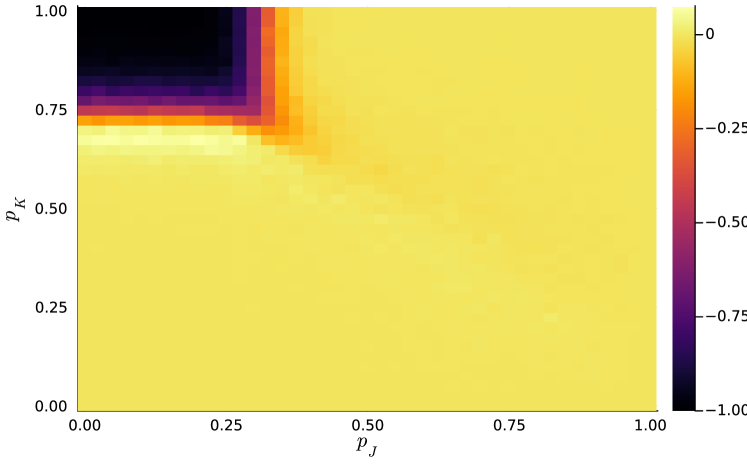
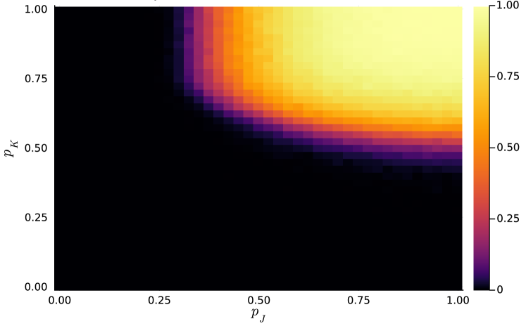
We scanned the 2d parameter space with $(L_{x},L_{y})=(12,7)$, $N_{t}=10$, and $N_{s}=1500$ to confirm the overall picture in Fig. 2. We refer to Fig. 5 for our results. Non-zero TEE, i.e., the existence of topological order, is displayed in a finite region close to $(p_{J},p_{K})=(0,1)$. Our key observation here is that the essential structure does not differ between the $N_{t}=10$ full-cycle scenario versus the measuring TEE in the middle after a further half-cycle with (1-1) and (1-2). The TEE is a robust measure of the deconfining phase of our MOC model, in this sense. We will see below that the precise phase boundary changes slightly as we increase the system size.

(a)

(b)

Figure 5: Topological entanglement entropy for our model with $(L_{x},L_{y})=(12,7)$, $N_{s}=1500$. (a) After 10 full cycles. (b) After 10 full cycles and a half cycle with steps (1-1) and (1-2). Both scenarios exhibit the deconfining phase at the top left corner.

We performed our numerical computation for $(L_{x},L_{y})=(12,6)$, $(16,8)$, $(20,10)$, $(24,12)$, and $(28,14)$. We set the number of measurement rounds to be $N_{t}=20$, so the spacetime volume of our system can be viewed as three dimensions. We checked by numerics that the entanglement measures converge to their equilibrium within $N_{t}\sim 10$ time steps. We performed the simulation at each parameter point with $N_{s}\sim 200$ samples. We conducted numerical simulations along several ‘cuts’ along lines in the parameter space. We refer to Fig. 6 for our main numerical result.

Figure 6: Results of our numerical simulations. (a) We scan simulations along various lines across the phase diagram. The labels (i)-(vii) represent different sub-manifolds in the two-dimensional parameter space spanned by $(p_{J},p_{K})$. (b)-(j) We present the result of each scan over varied probabilities along each line in Subfigure (a). Each result is obtained for the projective-gauge-Higgs MOC with $N_{t}=20$ time steps and averaged over $N_{s}=200$ samples.

As we increase the lattice sizes, the boundary of the topological order becomes sharper. To summarize key features, we have observed:

• Along (i), we see a critical point at $p^{c}_{J}\simeq 0.25$ along $p_{K}=1$.

• Along (ii), we see a critical point at $p^{c}_{K}\simeq 0.75$ along $p_{J}=1$.

• Along (iii), we see a transition point at $p^{c}_{K}$ which is slightly smaller than $0.75$, indicating a ‘cusp’ of the plateau of the deconfining phase penetrating towards the center of the phase diagram.

• Along (iv), we see a dip at $p_{J}\simeq 0.25$, consistent with the picture that a cusp exists at the right bottom corner of the deconfining phase.

II.3.2 Boundary mutual information

To compute the boundary mutual information $I(A:B)$, we take regions $A$ and $B$ in such a way that they contain the vertices at $(x,y)=(2,1)$ and $(x,y)=(L_{x}-1,1)$, respectively. Each of the regions also contains the adjacent edge on the rough boundary. We illustrate the setup in Fig. 4.

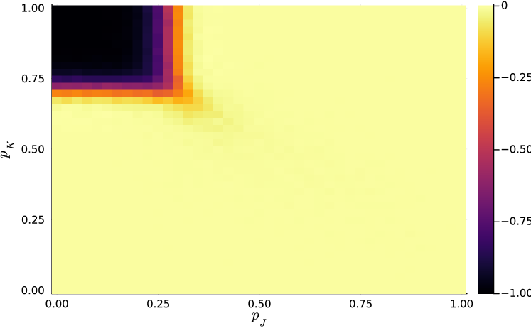
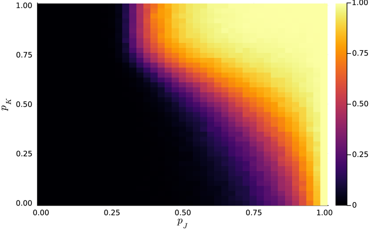
Similarly to the TEE, we scanned the 2d parameter space with $(L_{x},L_{y})=(12,7)$, $N_{t}=10$, and $N_{s}=1500$ to confirm the overall picture in Fig. 2. We refer to Fig. 7 for our results. The region with the non-zero BMI is exhibited over a finite region that contains the cluster state point $(p_{J},p_{K})=(1,1)$. We observe that the essential structure does not differ between the $N_{t}=10$ full-cycle scenario versus the measuring BMI in the middle after a further half-cycle with (1-1) and (1-2). Although the actual values of the BMI itself differ between the two scenarios, the onset of nonzero values agree roughly. We believe that the phase boundaries from the two scenarios match in the large system limit. It is worth mentioning that the BMI measured at the full cycles plus a half appears sharper; see Fig. 7.

(a)

(b)

Figure 7: Boundary mutual information for our model with $(L_{x},L_{y})=(12,7)$, $N_{s}=1500$. (a) After 10 full cycles. (b) After 10 full cycles and a half with steps (1-1) and (1-2). Both scenarios exhibit the Higgs=SPT phase at the finite region in the top right area.

We also performed our numerical computation with $N_{t}=20$ for $(L_{x},L_{y})=(12,6)$, $(16,8)$, $(20,10)$, $(24,12)$, and $(28,14)$. From the behavior of the BMI, we have observed a second-order-like phase transitions. As we increase the lattice sizes, the curve appears identical for different lattice sizes to the precision of our numerics. We have observed:

• Along (i), we see a critical point close to $p^{c}_{J}\simeq 0.25$ along $p_{K}=1$. We have not excluded a possibility that there is an intermediate phase between the deconfining phase and the Higgs=SPT phase, but we conjecture that the two boundaries match.

• Along (iv), we see a critical point at $p^{c}_{J}\simeq 0.3$. This can be compared with the rise of the TEE around that value in Fig. 6(g). This is consistent with a picture that the Higgs phase and the deconfining phase are mutually exclusive.

• Along (v), we see a transition point at $p^{c}_{K}=p^{c}_{K}\simeq$ slightly larger than 0.5, indicating that the Higgs phase extends almost to the center of the phase diagram.

• Along (vi), we see a critical point at $p^{c}_{K}\simeq 0.5$ along $p_{J}=1$.

• Along (vii), we see a critical point around $p^{c}_{K}\simeq 0.5$ along $p_{J}=0.75$, indicating that the phase boundary is almost flat horizontally starting from $(p_{J},p_{K})=(1,0.5)$.

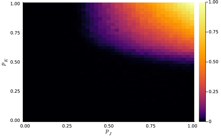
II.3.3 A mixed phase: open Wilson line operator in the bulk

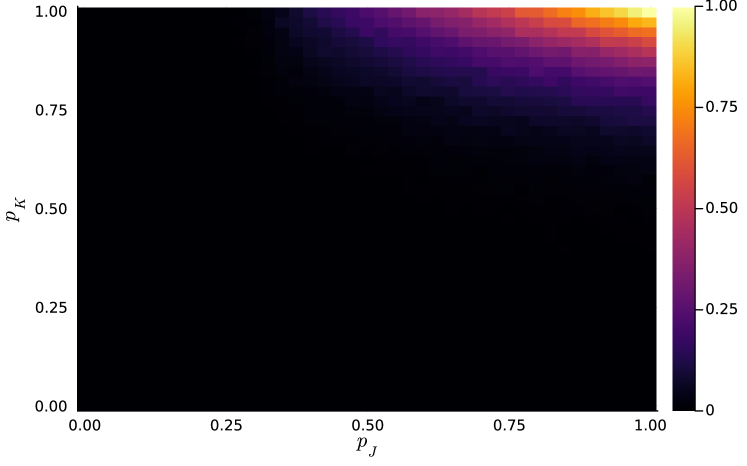
Next we probe different phases appearing alternately in the protocol. We run numerical simulations for the system with $(L_{x},L_{y})=(12,7)$ with $N_{t}=10$ full cycles. We measure the open Wilson line operator inserted at the middle of the lattice extended in the $x$ direction with length $7$; see Fig. 8.

Figure 8: A setup for the open Wilson line operator $W_{\gamma}$.

(a)

(b)

Figure 9: The averaged absolute value of open Wilson line operator for our model with $(L_{x},L_{y})=(12,7)$, $N_{s}=1500$. (a) After 10 full cycles. Only concentrated region around the cluster state point shows non-zero values. (b) After 10 full cycles and a half cycle with steps (1-1) and (1-2). A large region reaching to the boundary to the deconfining phase shows non-zero expectation values. The two scenarios show different structures, exhibiting the mixed phase.

First, we computed the expectation value $\mathbb{E}|\langle W_{\gamma}\rangle|$ after the $N_{t}=10$ full cycles. We observe non-zero expectation values concentrated around the cluster state point $(p_{J},p_{K})=(1,1)$, see Fig. 9(a).

When we stop at a half cycle (after several full cycles), the measured Wilson line operator becomes nonzero in a much wider region, extending all the way to $(p_{J},p_{K})=(1,0)$ point, as well as reaching the boundary to the deconfined phase, see Fig. 9(b). We also computed the dependence on the length of the Wilson line operator, and found that the smaller the length is, the larger the non-zero value region becomes.

In particular, we refer to the region near $(p_{J},p_{K})=(1,0)$ as a mixed region, as it exhibits either more Higgs-like property or more confinement property, depending how we stop the measurement cycle. This is in some sense analogous to mixture of water-vapor phase in the first-order transition. In contrast, near the other three corners, the properties seem stable regardless of how we stop the procedure.

II.4 Bulk phase transition, percolation, and duality

We have obtained the transition point $p_{K}\simeq 0.75$ at $p_{J}=0$ and $p_{J}\simeq 0.25$ at $p_{K}=1$ from the topological entanglement entropy. Below, we provide some explanation of the above results from the viewpoint of percolation and duality.

We first look at the transition point along the $p_{J}=0$ line. What is effectively simulated along this line is the MOC with $P^{(1)}_{B,p}$ (measuring the magnetic plaquette operator) and $P^{(3)}_{X,e}$ (measuring the electric link operator), as the vertex degrees of freedom is frozen to $X_{v}=1$ as a separate product state. This is a pure-gauge MOC model: (0) Initialize a 2d state in the product state $|+\rangle^{\otimes E}$. (2) Associated with each plaquette, measure $B_{p}$ with probability $p_{K}$. (3) Associated with each edge, measure $X_{e}$ with probability $1-p_{K}$, and so on. The simulated state obeys the Gauss law constraint $A_{v}=1$ for all $v\in V$, where $A_{v}$ is the star term in the toric code,

$$A_{v} =\prod_{e\supset v}X_{e}=\raisebox{-20.0pt}{ \leavevmode\hbox to44.19pt{\vbox to41.95pt{\pgfpicture\makeatletter\hbox{\hskip 22.0941pt\lower-20.97604pt\hbox to0.0pt{\pgfsys@beginscope\pgfsys@invoke{ }\definecolor{pgfstrokecolor}{rgb}{0,0,0}\pgfsys@color@rgb@stroke{0}{0}{0}\pgfsys@invoke{ }\pgfsys@color@rgb@fill{0}{0}{0}\pgfsys@invoke{ }\pgfsys@setlinewidth{0.4pt}\pgfsys@invoke{ }\nullfont\pgfsys@beginscope\pgfsys@invoke{ }\pgfsys@invoke{\lxSVG@closescope }\pgfsys@endscope\hbox to0.0pt{\pgfsys@beginscope\pgfsys@invoke{ }{}{{}}{} {}{}\pgfsys@beginscope\pgfsys@invoke{ }\color[rgb]{0.7,0.7,0.7}\definecolor[named]{pgfstrokecolor}{rgb}{0.7,0.7,0.7}\pgfsys@color@gray@stroke{0.7}\pgfsys@invoke{ }\pgfsys@color@gray@fill{0.7}\pgfsys@invoke{ }\definecolor{pgffillcolor}{rgb}{0.7,0.7,0.7}\pgfsys@setlinewidth{1.0pt}\pgfsys@invoke{ }{}\pgfsys@moveto{-14.22638pt}{0.0pt}\pgfsys@lineto{14.22638pt}{0.0pt}\pgfsys@stroke\pgfsys@invoke{ } \pgfsys@invoke{\lxSVG@closescope }\pgfsys@endscope{}{{}}{} {}{}\pgfsys@beginscope\pgfsys@invoke{ }\color[rgb]{0.7,0.7,0.7}\definecolor[named]{pgfstrokecolor}{rgb}{0.7,0.7,0.7}\pgfsys@color@gray@stroke{0.7}\pgfsys@invoke{ }\pgfsys@color@gray@fill{0.7}\pgfsys@invoke{ }\definecolor{pgffillcolor}{rgb}{0.7,0.7,0.7}\pgfsys@setlinewidth{1.0pt}\pgfsys@invoke{ }{}\pgfsys@moveto{0.0pt}{-14.22638pt}\pgfsys@lineto{0.0pt}{14.22638pt}\pgfsys@stroke\pgfsys@invoke{ } \pgfsys@invoke{\lxSVG@closescope }\pgfsys@endscope{{}}\hbox{\hbox{{\pgfsys@beginscope\pgfsys@invoke{ }{{}{}{{ {}{}}}{ {}{}} {{}{{}}}{{}{}}{}{{}{}} { }{{{{}}\pgfsys@beginscope\pgfsys@invoke{ }\pgfsys@transformcm{1.0}{0.0}{0.0}{1.0}{-18.7611pt}{-3.41666pt}\pgfsys@invoke{ }\hbox{{\definecolor{pgfstrokecolor}{rgb}{0,0,0}\pgfsys@color@rgb@stroke{0}{0}{0}\pgfsys@invoke{ }\pgfsys@color@rgb@fill{0}{0}{0}\pgfsys@invoke{ }\hbox{{$X$}} }}\pgfsys@invoke{\lxSVG@closescope }\pgfsys@endscope}}} \pgfsys@invoke{\lxSVG@closescope }\pgfsys@endscope}}} {{}}\hbox{\hbox{{\pgfsys@beginscope\pgfsys@invoke{ }{{}{}{{ {}{}}}{ {}{}} {{}{{}}}{{}{}}{}{{}{}} { }{{{{}}\pgfsys@beginscope\pgfsys@invoke{ }\pgfsys@transformcm{1.0}{0.0}{0.0}{1.0}{9.69167pt}{-3.41666pt}\pgfsys@invoke{ }\hbox{{\definecolor{pgfstrokecolor}{rgb}{0,0,0}\pgfsys@color@rgb@stroke{0}{0}{0}\pgfsys@invoke{ }\pgfsys@color@rgb@fill{0}{0}{0}\pgfsys@invoke{ }\hbox{{$X$}} }}\pgfsys@invoke{\lxSVG@closescope }\pgfsys@endscope}}} \pgfsys@invoke{\lxSVG@closescope }\pgfsys@endscope}}} {{}}\hbox{\hbox{{\pgfsys@beginscope\pgfsys@invoke{ }{{}{}{{ {}{}}}{ {}{}} {{}{{}}}{{}{}}{}{{}{}} { }{{{{}}\pgfsys@beginscope\pgfsys@invoke{ }\pgfsys@transformcm{1.0}{0.0}{0.0}{1.0}{-4.53471pt}{10.80972pt}\pgfsys@invoke{ }\hbox{{\definecolor{pgfstrokecolor}{rgb}{0,0,0}\pgfsys@color@rgb@stroke{0}{0}{0}\pgfsys@invoke{ }\pgfsys@color@rgb@fill{0}{0}{0}\pgfsys@invoke{ }\hbox{{$X$}} }}\pgfsys@invoke{\lxSVG@closescope }\pgfsys@endscope}}} \pgfsys@invoke{\lxSVG@closescope }\pgfsys@endscope}}} {{}}\hbox{\hbox{{\pgfsys@beginscope\pgfsys@invoke{ }{{}{}{{ {}{}}}{ {}{}} {{}{{}}}{{}{}}{}{{}{}} { }{{{{}}\pgfsys@beginscope\pgfsys@invoke{ }\pgfsys@transformcm{1.0}{0.0}{0.0}{1.0}{-4.53471pt}{-17.64304pt}\pgfsys@invoke{ }\hbox{{\definecolor{pgfstrokecolor}{rgb}{0,0,0}\pgfsys@color@rgb@stroke{0}{0}{0}\pgfsys@invoke{ }\pgfsys@color@rgb@fill{0}{0}{0}\pgfsys@invoke{ }\hbox{{$X$}} }}\pgfsys@invoke{\lxSVG@closescope }\pgfsys@endscope}}} \pgfsys@invoke{\lxSVG@closescope }\pgfsys@endscope}}} \pgfsys@invoke{\lxSVG@closescope }\pgfsys@endscope{}{}{}\hss}\pgfsys@discardpath\pgfsys@invoke{\lxSVG@closescope }\pgfsys@endscope\hss}}\lxSVG@closescope\endpgfpicture}} }\quad\forall v\in V. X X X X X X X X$$ (18)

In Appendix C, generalizing the relation between the bond percolation and pTFI, we argue that a phase transition in the pure gauge MOC can be described by a homological percolation [76, 77] of surfaces in the 3d square lattice. Indeed, the surface percolation in 3d lattice is dual to the bond percolation with a relation in thresholds $\tilde{p}^{\text{bond}}_{c}+\tilde{p}^{\text{surface}}_{c}=1$ (see [76, 77]). According to Refs. [78, 79], $\tilde{p}^{\rm bond}_{c}=0.2488126(5)$, so our phase transition at $p_{K}\simeq 0.75$ is consistent with the surface percolation threshold.

For the transition along the $p_{K}=1$ line, we use a duality to consider an equivalent model. Consider a map

$$\mathbf{\Sigma}=\langle+|^{\otimes V}\prod_{\langle e,v\rangle}CX_{v,e},$$ (19)

where $\prod_{\langle e,v\rangle}$ is the product over adjacent pairs of vertices and edges and $CX_{a,b}$ is the controlled-$X$ operator, $CX_{a,b}=|0\rangle\langle 0|_{a}\otimes I_{b}+|1\rangle\langle 1|_{a}\otimes X_{b}$. Then, the measurement bases on the $p_{K}=1$ line are mapped as follows:

$$\mathbf{\Sigma}\cdot\begin{pmatrix}X_{v}\\ W_{e}\\ B_{p}\end{pmatrix}=\begin{pmatrix}A_{v}\\ Z_{e}\\ B_{p}\end{pmatrix}\cdot\mathbf{\Sigma}.$$ (20)

Thus the projective gauge-Higgs MOC model with bases $(X_{v},W_{e},B_{p})$ and probability assignment $(1-p_{J},p_{J},1)$ is equivalent to that with $(A_{v},Z_{e},B_{p})$ and probability assignment $(1-p_{J},p_{J},1)$. By further transforming them using the Hadamard transform and viewing the terms as those in the dual lattice, we have an MOC model with $(B_{p^{*}},X_{e^{*}},A_{v^{*}})$ and probability assignment $(1-p_{J},p_{J},1)$. It is the pure-gauge MOC model that we described above (with a different initial state), and thus the transition point is expected at $1-p_{J}=\tilde{p}^{\text{surface}}_{c}$, so $p_{J}=\tilde{p}^{\text{bond}}_{c}$. This is consistent with our critical point, $p_{J}\simeq 0.25$.

We note that there is another map that we can make use of. The map is simply a projector

$$\mathbf{\Delta}=\langle 0|^{\otimes E}.$$ (21)

Essentially, the operator $\mathbf{\Delta}$ forces to solve for the Gauss law constraints in the gauge theory and leaves us a model without gauge redundancy but with the $\mathbb{Z}_{2}$ global symmetry. We get

$$\mathbf{\Delta}\cdot\begin{pmatrix}X_{v}\\ W_{e}\\ B_{p}\end{pmatrix}=\begin{pmatrix}X_{v}\\ L_{e}\\ I\end{pmatrix}\cdot\mathbf{\Delta}$$ (22)

with $L_{e}=\prod_{v\subset e}Z_{v}$ being the Ising interaction,

$$L_{e} =\prod_{v\subset e}Z_{v}=\raisebox{-10.0pt}{ \leavevmode\hbox to52.21pt{\vbox to23.76pt{\pgfpicture\makeatletter\hbox{\hskip 11.88092pt\lower-11.88092pt\hbox to0.0pt{\pgfsys@beginscope\pgfsys@invoke{ }\definecolor{pgfstrokecolor}{rgb}{0,0,0}\pgfsys@color@rgb@stroke{0}{0}{0}\pgfsys@invoke{ }\pgfsys@color@rgb@fill{0}{0}{0}\pgfsys@invoke{ }\pgfsys@setlinewidth{0.4pt}\pgfsys@invoke{ }\nullfont\pgfsys@beginscope\pgfsys@invoke{ }\pgfsys@invoke{\lxSVG@closescope }\pgfsys@endscope\hbox to0.0pt{\pgfsys@beginscope\pgfsys@invoke{ }{}{{}}{} {}{}\pgfsys@beginscope\pgfsys@invoke{ }\color[rgb]{0.7,0.7,0.7}\definecolor[named]{pgfstrokecolor}{rgb}{0.7,0.7,0.7}\pgfsys@color@gray@stroke{0.7}\pgfsys@invoke{ }\pgfsys@color@gray@fill{0.7}\pgfsys@invoke{ }\definecolor{pgffillcolor}{rgb}{0.7,0.7,0.7}\pgfsys@setlinewidth{1.0pt}\pgfsys@invoke{ }{}\pgfsys@moveto{-11.38092pt}{0.0pt}\pgfsys@lineto{39.83368pt}{0.0pt}\pgfsys@stroke\pgfsys@invoke{ } \pgfsys@invoke{\lxSVG@closescope }\pgfsys@endscope{}{{}}{} {}{}\pgfsys@beginscope\pgfsys@invoke{ }\color[rgb]{0.7,0.7,0.7}\definecolor[named]{pgfstrokecolor}{rgb}{0.7,0.7,0.7}\pgfsys@color@gray@stroke{0.7}\pgfsys@invoke{ }\pgfsys@color@gray@fill{0.7}\pgfsys@invoke{ }\definecolor{pgffillcolor}{rgb}{0.7,0.7,0.7}\pgfsys@setlinewidth{1.0pt}\pgfsys@invoke{ }{}\pgfsys@moveto{0.0pt}{-11.38092pt}\pgfsys@lineto{0.0pt}{11.38092pt}\pgfsys@stroke\pgfsys@invoke{ } \pgfsys@invoke{\lxSVG@closescope }\pgfsys@endscope{}{{}}{} {}{}\pgfsys@beginscope\pgfsys@invoke{ }\color[rgb]{0.7,0.7,0.7}\definecolor[named]{pgfstrokecolor}{rgb}{0.7,0.7,0.7}\pgfsys@color@gray@stroke{0.7}\pgfsys@invoke{ }\pgfsys@color@gray@fill{0.7}\pgfsys@invoke{ }\definecolor{pgffillcolor}{rgb}{0.7,0.7,0.7}\pgfsys@setlinewidth{1.0pt}\pgfsys@invoke{ }{}\pgfsys@moveto{28.45276pt}{-11.38092pt}\pgfsys@lineto{28.45276pt}{11.38092pt}\pgfsys@stroke\pgfsys@invoke{ } \pgfsys@invoke{\lxSVG@closescope }\pgfsys@endscope{{}}\hbox{\hbox{{\pgfsys@beginscope\pgfsys@invoke{ }{{}{}{{ {}{}}}{ {}{}} {{}{{}}}{{}{}}{}{{}{}} { }{{{{}}\pgfsys@beginscope\pgfsys@invoke{ }\pgfsys@transformcm{1.0}{0.0}{0.0}{1.0}{24.68193pt}{-3.41666pt}\pgfsys@invoke{ }\hbox{{\definecolor{pgfstrokecolor}{rgb}{0,0,0}\pgfsys@color@rgb@stroke{0}{0}{0}\pgfsys@invoke{ }\pgfsys@color@rgb@fill{0}{0}{0}\pgfsys@invoke{ }\hbox{{$Z$}} }}\pgfsys@invoke{\lxSVG@closescope }\pgfsys@endscope}}} \pgfsys@invoke{\lxSVG@closescope }\pgfsys@endscope}}} {{}}\hbox{\hbox{{\pgfsys@beginscope\pgfsys@invoke{ }{{}{}{{ {}{}}}{ {}{}} {{}{{}}}{{}{}}{}{{}{}} { }{{{{}}\pgfsys@beginscope\pgfsys@invoke{ }\pgfsys@transformcm{1.0}{0.0}{0.0}{1.0}{-3.77083pt}{-3.41666pt}\pgfsys@invoke{ }\hbox{{\definecolor{pgfstrokecolor}{rgb}{0,0,0}\pgfsys@color@rgb@stroke{0}{0}{0}\pgfsys@invoke{ }\pgfsys@color@rgb@fill{0}{0}{0}\pgfsys@invoke{ }\hbox{{$Z$}} }}\pgfsys@invoke{\lxSVG@closescope }\pgfsys@endscope}}} \pgfsys@invoke{\lxSVG@closescope }\pgfsys@endscope}}} \pgfsys@invoke{\lxSVG@closescope }\pgfsys@endscope{}{}{}\hss}\pgfsys@discardpath\pgfsys@invoke{\lxSVG@closescope }\pgfsys@endscope\hss}}\lxSVG@closescope\endpgfpicture}} }. Z Z Z Z$$ (23)

Therefore, the projective gauge-Higgs MOC model with measurement bases $(W_{e},X_{v},B_{p})$ and probability assignment $(p_{J},1-p_{J},1)$ is equivalent to that with $(X_{v},L_{e})$ and probability assignment $(p_{J},1-p_{J})$. The latter model is the $(2+1)$d pTFI model, which was also studied by Lang and Büchler. Their numerical result and the percolation picture indicated that the transition point is at the 3d bond percolation threshold $\tilde{p}^{\rm 3d}_{c}=0.2488126(5)$ for the square lattice. This is consistent with our numerical result of critical $p_{J}\simeq 0.25$ at $p_{K}=1$. Conceptual connection to the topological entanglement entropy is obfuscated in this picture, however.

II.5 Boundary phase transition and percolation via screening

Next, we unmask the physics behind the boundary phase transitions. Along the $p_{K}=1$ line, we had a transition at $p_{J}\simeq 0.25$, consistent with the fact that an SPT phase is short-range entangled, so it cannot coexist with the deconfining phase. How about the $p_{J}=1$ line, where we observed a transition at $p_{K}\simeq 0.5$? Below, we claim that the effective theory is a boundary $(1+1)$d pTFI model and the bulk is effectively decoupled, so the critical point is that of the $(1+1)$d pTFI in disguise.

To derive the effective theory, we use the cluster state entangler

$$\mathbf{\mathcal{C}}=\prod_{\langle e,v\rangle}CX_{v,e}.$$ (24)

Then the measurement bases relevant in the $p_{J}=1$ line are transformed as

(25)

(26)

(27)

The measurement with the basis (25) occurs with the unit probability in the bulk (due to $p_{J}=1$ in the original theory), so the $Z$ measurement round is trivial in the sense that the plaquette operator $B_{p}$ is locked to $B_{p}=1$. Therefore, the bulk system in this basis experiences no entangling dynamics; it is simply a cycle of (1) reset to $Z_{e}=1$ (2) measure $X_{e}$ with probability $1-p_{K}$.

The plaquette opeator on the boundary, on the other hand, is non-trivial. We get

(28)

for $p\in P_{\partial}$. In the equality, we used the condition $Z_{e}=1$ ($e\in E_{B}$) from the bulk measurement with unit probability. The measurement with the basis (28) occurs with the probability $p_{K}$, and that with the basis $X_{e}$ $(e\in E_{\partial})$ takes place with the probability $1-p_{K}$. Hence, we conclude that the effective theory related to the projective gauge-Higgs MOC model at $p_{J}=1$ via $\mathbf{\mathcal{C}}$ is:

• the decoupled bulk system with a cycle of single qubit measurement of $X_{e}$ and resetting to $Z_{e}=1$,

• the boundary $(1+1)$d MOC circuit with the Ising basis (28) with probability $p_{K}$ and the single-qubit basis $X_{e}$ with probability $1-p_{K}$, i.e., the 1d pTFI model.

The critical measurement rate of the 1d pTFI is $0.5$ (the percolation threshold on the 2d square lattice), and our result of critical $p_{K}\simeq 0.5$ along $p_{J}=1$ is consistent.

III Conclusions and discussion

In this work, we considered an MOC model inspired by the Fradkin-Shenker model. We computed the topological entanglement entropy to diagnose the topological order in the simulated state, and we found a clear phase transition across varied measurement rates. Further, motivated by the recent finding of the boundary symmetry-breaking order, we diagnosed such a boundary long-range order by mutual information. The structure of our phase diagram is consistent with the one obtained from the corresponding models via the numerical DMRG method [64], for example.

The above two topological phases, either intrinsic or symmetry-protected, are robust entanglement orders of our MO Fradkin-Shenker model. We also showed that our MO circuit exhibits a mixed phase, which corresponds to the parameter regime with frustrated terms in the quantum Hamiltonian picture. The bulk open Wilson line operator detects states alternating over measurement rounds, wherein we saw a continuity between the Higgs limit and the confining limit as well as a clear separation from the deconfining phase.

Our results suggest that it will be possible to realize the Higgs=SPT phenomenon on quantum devices in the near future. Recent progress in quantum technology has allowed us to program mid-circuit measurements in quantum devices, such as superconducting or trapped-ion processors. Some of other devices that allow mid-circuit measurements, such as reconfigurable atom arrays, may not support the universal quantum computation, but they would still be useful for realizing MOC models. Although quantum operations are still noisy as of present, it is worth noting that one can translate an MOC model into an MBQC model, as discussed in Appendix C. There, the resource state (in one dimension higher) can be prepared with a constant-depth unitary circuit, and an MOC circuit can be simulated by Pauli-basis measurements in the bulk, with the output state induced at the boundary of the resource state. Crucially, one can perform the bulk measurements simultaneously as we do not need to implement $SU(2)$ gates, which will reduce the circuit complexity to constant. Hence, it is speculated that studies of MOC models on experimental platforms are not so far-fetched within the near-future technology. The resource state for simulating the Fradkin-Shenker model was proposed by one of us in Ref. [80]. A related idea was also explored by Liu et al. [38].

One intriguing open question is whether there is a multi-critical point in the MOC phase diagram as found in the 3d Euclidean lattice field theory of the Fradkin-Shenker model [63]. Answering this question, of course, requires much more numerical effort. It would also be useful to understand the relation between the ordinary 3d Euclidean path integral and the replica manifold for entanglement entropy of MOCs, as well as the role of the duality in entanglement spectrum [81]. We hope to advance our study in this direction in the future.

Note added: Recently, a paper appeared on arXiv [71], where authors made the connection between the gauge-Higgs model and percolation. We deduced a connection to percolation based on an MBQC picture.

Appendix A Stabilizer update algorithm

The algorithm for updating stabilizers can be found in Ref. [24], for example. Consider a state uniquely specified by stabilizers $S=\langle g_{1},...,g_{p}\rangle$ and measuring an operator $\tilde{g}$. (That is, $\tilde{g}=B_{p}$ in the measurement (1-1), for example.)

1. Search in $\{g_{1},...,g_{p}\}$ an element that anti-commutes with $\tilde{g}$. Let $g_{k}$ be that operator and go to 3.

2. This is the case when $\tilde{g}$ commutes with all the elements in $S$. If $\tilde{g}$ or $-\tilde{g}$ is an element in $S$, then the measurement outcome is deterministic and the resulting stabilizer set remains $S$. Otherwise, update the stabilizer set to $\{g_{1},...,g_{p},(-1)^{m}\tilde{g}\}$, where $m=0,1$ is the measurement outcome. When the size of the stabilizer generators is the same as the number of qubits, then the second operation does not take place since the number of stabilizer should not increase.

3. Swap $g_{1}$ and $g_{k}$.

4. For $j=2,...,p$, check if $\tilde{g}$ anti-commutes with $g_{i}$, and if it does, update $g_{i}\mapsto g_{1}g_{i}$. (After this, $g_{1}$ is the only operator non-commuting with $\tilde{g}$.)

5. Measure $\tilde{g}$ with a random outcome $m$. (Both outcomes appear with an equality probability of $1/2$.) Update the stabilizer set to $\{(-1)^{m}\tilde{g},g_{2},...,g_{p}\}$.

Example. If we start with a four-edge, four-vertex product state on a square, we have $S=\langle X_{1},X_{2},X_{3},X_{4},\tilde{X}_{1},\tilde{X}_{2},\tilde{X}_{3},\tilde{X}_{4}\rangle$. We have represented the edge d.o.f. with tilde. Consider measuring the plaquette operator $\tilde{g}=\tilde{Z}_{1}\tilde{Z}_{2}\tilde{Z}_{3}\tilde{Z}_{4}$. Then the algorithm goes as follows. (1) We find an anti-commuting element $\tilde{X}_{1}$, $\{\tilde{X}_{1},\tilde{g}\}=0$, i.e., “$g_{k}=\tilde{X}_{1}$.” (3) Swap $g_{1}=X_{1}$ with $g_{k}=\tilde{X}_{1}$. We have $S=\langle\tilde{X}_{1},X_{2},X_{3},X_{4},X_{1},\tilde{X}_{2},\tilde{X}_{3},\tilde{X}_{4}\rangle$. (4) In the right of the first element, we find $\tilde{X}_{2},\tilde{X}_{3},\tilde{X}_{4}$ anti-commute with $\tilde{g}=\tilde{Z}_{1}\tilde{Z}_{2}\tilde{Z}_{3}\tilde{Z}_{4}$. We update as $S=\langle\tilde{X}_{1},X_{2},X_{3},X_{4},X_{1},\tilde{X}_{1}\tilde{X}_{2},\tilde{X}_{1}\tilde{X}_{3},\tilde{X}_{1}\tilde{X}_{4}\rangle$. (5) Now we replace $g_{1}$ with $\tilde{g}$ due to the measurement, and all the other elements are unaffected since they commute with $\tilde{g}$: $S=\langle(-1)^{m}\tilde{Z}_{1}\tilde{Z}_{2}\tilde{Z}_{3}\tilde{Z}_{4},X_{2},X_{3},X_{4},X_{1},\tilde{X}_{1}\tilde{X}_{2},\tilde{X}_{1}\tilde{X}_{3},\tilde{X}_{1}\tilde{X}_{4}\rangle$, where $m$ denotes the measurement outcome.

Appendix B Entanglement entropy from stabilizers

To compute the entanglement entropy from stabilizers, we can employ the result by Hamma et al. [75]. Here, we follow the description in Appendix C of Ref. [16]. Consider a subsystem $A$, and let $I_{A}$ be the number of independent stabilizers when restricted to the region $A$. The entanglement entropy is given by the following formula:

$$S_{A}=I_{A}-|A|\ .$$ (29)

Let us express the stabilizer using a $\mathbb{Z}_{2}=\{0,1\}$ vector as

$$S_{j}=X^{\vec{v}_{j}}Z^{\vec{w}_{j}}\ ,$$ (30)

with $\vec{v}_{j},\vec{w}_{j}\in\{0,1\}^{N}$ being row vectors. We construct a vector

$$\vec{s}_{j}=(\vec{v}_{j},\vec{w}_{j})\ .$$ (31)

Now we have a matrix at each time step

$$\Psi(t)=(\vec{s}^{\,1T},\vec{s}^{\,2T},...,\vec{s}^{\,|\mathcal{S}|T})\ .$$ (32)

Each column is a stabilizer and each row represents a Pauli. Now $I_{A}$ is equivalent to the rank of the matrix $\Psi_{A}$ after deleting rows corresponding to $\bar{A}$.

$$I_{A}=\text{rank}(\Psi(t)_{A})\ .$$ (33)

Appendix C Pure-gauge MOC by measuring the RBH model

In this Appendix, we consider the pure-gauge MOC circuit and relate it to the 3d surface percolation via a perspective of Measurement-Based Quantum Computation (MBQC) [56, 58] on the Raussendorf-Bravyi-Harrington (RBH) state [82]. We consider the 3d cubic lattice, and place qubits in the eigenstate $|+\rangle$ on faces and edges of it. We adopt a notation where the bold font denotes cells in the 3d lattice, while the ordinary font represents a cell in the $xy$-plane projected to the $z$ direction. For instance, we write $\mathbf{f}=f\otimes\{z=0\}$ for a face within a $xy$-plane at $z=0$, and $\mathbf{f}=e\otimes[0,1]$ for a face extending in the $z$ direction; we also write $\mathbf{e}=e\otimes\{z=0\}$ for an edge within a $xy$-plane, and $\mathbf{e}=v\otimes[0,1]$ for an edge extending in the $z$ direction. Then the RBH state is defined as

$$|\psi_{\text{RBH}}\rangle\equiv\prod_{\langle\mathbf{e},\mathbf{f}\rangle}CZ_{\mathbf{e},\mathbf{f}}|+\rangle^{\otimes\mathbf{E}}|+\rangle^{\otimes\mathbf{F}}.$$ (34)

More precisely, we consider an open lattice with the range $z\in[0,L_{z}]$ and remove qubits on faces in the slice $z=L_{z}$.

We claim that the following measurements on the RBH state simulate the pure-gauge MOC model:

• Measure each of the $\mathbf{E}$ qubits in the $X$ basis with the unit probability.

• Measure each of the $\mathbf{F}$ qubits in the $X$ basis with the probability $p_{K}$; otherwise measure the qubit in the $Z$ basis.

• The $\mathbf{E}$ qubits at $z=L_{z}$ remain unmeasured, where the simulated state is induced.

As in the main text, we can restrict our attention to the quantum trajectory with all the measurement outcomes being $+1$.

To see the correspondence, let us consider the RBH state with qubits in $z<\ell\leq L_{z}$ having been already measured. We can write

$$|\psi_{\text{RBH}}(\ell)\rangle$$

$$=\prod_{\langle\mathbf{e},\mathbf{f}\rangle,z\geq\ell}CZ_{\mathbf{e},\mathbf{f}}|+\rangle^{\otimes\mathbf{E}}_{z>\ell}|+\rangle^{\otimes\mathbf{F}}_{z\geq\ell}\otimes|\Phi(\ell)\rangle_{\mathbf{E},z=\ell}\otimes|\text{junk}\rangle,$$ (35)

where $|\text{junk}\rangle$ is the normalized post-measurement product state in $z<\ell$ and $|\Phi(\ell)\rangle$ is the state on which we simulate the pure-gauge MOC. It satisfies the condition $A_{v}|\Phi(\ell)\rangle=|\Phi(\ell)\rangle$.

We set the bra state associated with the measurement within $\ell\leq z<\ell+1$ to be

$$\mathbb{M}_{\ell\leq z<\ell+1}=\Big{(}\prod_{\mathbf{e}\in\mathbf{E}}\langle+|\prod_{\mathbf{f}\in\mathbf{F}_{X}}\langle+|\prod_{\mathbf{f}\in\mathbf{F}_{Z}}\langle 0|\Big{)}\quad\Big{|}_{\ell\leq z<\ell+1}.$$ (36)

Here $\mathbf{F}_{X}$ ($\mathbf{F}_{Z}$) denotes the subset of faces where the measurement with the $X$ ($Z$) basis occurred. Then the state $\mathbb{M}_{\ell\leq z<\ell+1}|\psi_{\text{RBH}}(\ell)\rangle$ is equal to the state $|\psi_{\text{RBH}}(\ell+1)\rangle$ with the simulated state having evolved as

$$|\Phi(\ell+1)\rangle=\prod_{e\times[\ell,\ell+1]\in\mathbf{F}_{Z}}|+\rangle\langle 0|_{e}\prod_{e\times[\ell,\ell+1]\in\mathbf{F}_{X}}\frac{H_{e}}{\sqrt{2}}$$

$$\qquad\qquad\times\prod_{v\in V}\frac{1+\prod_{e\supset v}Z_{e}}{2}\prod_{e\in E}\frac{H_{e}}{\sqrt{2}}$$

$$\qquad\qquad\times\prod_{f\times\{\ell\}\in\mathbf{F}_{Z}}\frac{1}{\sqrt{2}}\prod_{f\times\{\ell\}\in\mathbf{F}_{X}}\frac{1+B_{f}}{2}|\Phi(\ell)\rangle$$

$$=\prod_{e\in E}\frac{1}{\sqrt{2}}\times\prod_{e\times[\ell,\ell+1]\in\mathbf{F}_{Z}}|+\rangle\langle+|_{e}\prod_{e\times[\ell,\ell+1]\in\mathbf{F}_{X}}\frac{1}{\sqrt{2}}$$

$$\times\prod_{f\times\{\ell\}\in\mathbf{F}_{Z}}\frac{1}{\sqrt{2}}\prod_{f\times\{\ell\}\in\mathbf{F}_{X}}\frac{1+B_{f}}{2}|\Phi(\ell)\rangle.$$ (37)

Thus one obtains a model where the measurement with $B_{f}$ occurs with probability $p_{K}$ and that with $X_{e}$ with probability $1-p_{K}$. We denote the entire measurement sequence as $\mathbb{M}=\prod_{\ell\in\{0,...,L_{z}-1\}}\mathbb{M}_{\ell\leq z<\ell+1}$, so that the simulated state in the end is $\mathbb{M}|\psi_{\text{RBH}}\rangle$.

We mentioned that the simulated state obeys the Gauss law constraint $A_{v}=+1$. The long-range order would be supported in coordination with the vacuum expectation value with respect to a non-local operator, i.e., $\langle W(\gamma)\rangle$ with $W(\gamma)$ a product of $Z$ operators along an arbitrarily large closed loop. We note that the RBH state is symmetric under a transformation supported on relative cycles $\mathbf{z}$, which is a sum of elements in $\mathbf{F}$ such that its boundary is a closed loop on $z=L_{z}$ (a closed surface in 3d which terminates on the boundary as a loop), i.e., $\partial\mathbf{z}=\gamma$:

$$\mathbf{W}(\mathbf{z})\equiv\prod_{\mathbf{f}\in\mathbf{z}}X_{\mathbf{f}}\times W(\gamma),$$ (38)

$$\mathbf{W}(\mathbf{z})|\psi_{\text{RBH}}\rangle=|\psi_{\text{RBH}}\rangle,$$ (39)

where, in the second equality, we have used that $\mathbf{W}(\mathbf{z})$ is a product of stabilizer operators of the RBH graph state. The condition is also known as the 1-form symmetry of the RBH state, see e.g., Ref. [83]. Hence, if a subset of $\mathbf{F}_{X}$ in our measurement forms relative cycles, it enforces correlation in the simulated state. Namely, if $\mathbf{z}$ can be formed by the cells in $\mathbf{F}_{X}$, then

$$\mathbb{M}\mathbf{W}(\mathbf{z})|\psi_{\text{RBH}}\rangle=\mathbb{M}W(\gamma)|\psi_{\text{RBH}}\rangle=\mathbb{M}|\psi_{\text{RBH}}\rangle,$$ (40)

so that $W(\gamma)$ becomes enforced in the simulated state.

Our equation (40) implies that if faces in $\mathbf{F}_{X}$ can form large cycles (closed surfaces, except those that terminate at the boundary), it is likely that the 2d simulated state hosts the deconfining order supported by large Wilson loops ($W(\gamma)=1$ for a large $\gamma$). Roughly speaking, the formation of giant cycles (closed surface consisting of faces) by cells each of which is activated with probability $p_{K}$ is the mathematical problem called homological percolation. One of its simplest versions in lower dimensions, e.g. in 2d, is the bond percolation problem, which is the underlying mechanism of the MIPT in the pTFI model [47]. The spacetime picture we provided here is a generalization of theirs, phrased in the language of MBQC. We speculate that the transition to the deconfining phase occurs as the consequence of the homological percolation formed by $X$ measurements on the RBH state.

Figure 10: The unit cell in the RBH state. Qubits are placed on the edges and faces of the 3d cubic lattice, and $CZ$ gates are applied to adjacent qubits as drawn in green. Note that we place $z=0$ at the top and the simulated time direction goes from the top to bottom.

References

- Bravyi et al. [2006] S. Bravyi, M. B. Hastings, and F. Verstraete, Lieb-Robinson Bounds and the Generation of Correlations and Topological Quantum Order, Phys. Rev. Lett. 97, 050401 (2006), arXiv:quant-ph/0603121 [quant-ph] .
- Chen et al. [2010] X. Chen, Z.-C. Gu, and X.-G. Wen, Local unitary transformation, long-range quantum entanglement, wave function renormalization, and topological order, Phys. Rev. B 82, 155138 (2010), arXiv:1004.3835 [cond-mat.str-el] .
- Kitaev [2003] A. Y. Kitaev, Fault-tolerant quantum computation by anyons, Annals of Physics 303, 2 (2003), arXiv:quant-ph/9707021 [quant-ph] .
- Levin and Wen [2005] M. A. Levin and X.-G. Wen, String-net condensation: A physical mechanism for topological phases, Phys. Rev. B 71, 045110 (2005), arXiv:cond-mat/0404617 [cond-mat.str-el] .
- Gu and Wen [2009] Z.-C. Gu and X.-G. Wen, Tensor-entanglement-filtering renormalization approach and symmetry-protected topological order, Phys. Rev. B 80, 155131 (2009), arXiv:0903.1069 [cond-mat.str-el] .
- Pollmann et al. [2012] F. Pollmann, E. Berg, A. M. Turner, and M. Oshikawa, Symmetry protection of topological phases in one-dimensional quantum spin systems, Phys. Rev. B 85, 075125 (2012), arXiv:0909.4059 [cond-mat.str-el] .
- Pollmann et al. [2010] F. Pollmann, A. M. Turner, E. Berg, and M. Oshikawa, Entanglement spectrum of a topological phase in one dimension, Phys. Rev. B 81, 064439 (2010), arXiv:0910.1811 [cond-mat.str-el] .
- Chen et al. [2011a] X. Chen, Z.-C. Gu, and X.-G. Wen, Classification of gapped symmetric phases in one-dimensional spin systems, Phys. Rev. B 83, 035107 (2011a), arXiv:1008.3745 [cond-mat.str-el] .
- Chen et al. [2011b] X. Chen, Z.-X. Liu, and X.-G. Wen, Two-dimensional symmetry-protected topological orders and their protected gapless edge excitations, Phys. Rev. B 84, 235141 (2011b), arXiv:1106.4752 [cond-mat.str-el] .
- Chen et al. [2011c] X. Chen, Z.-C. Gu, and X.-G. Wen, Complete classification of one-dimensional gapped quantum phases in interacting spin systems, Phys. Rev. B 84, 235128 (2011c), arXiv:1103.3323 [cond-mat.str-el] .
- Schuch et al. [2011] N. Schuch, D. Pérez-García, and I. Cirac, Classifying quantum phases using matrix product states and projected entangled pair states, Phys. Rev. B 84, 165139 (2011), arXiv:1010.3732 [cond-mat.str-el] .
- Chen et al. [2013] X. Chen, Z.-C. Gu, Z.-X. Liu, and X.-G. Wen, Symmetry protected topological orders and the group cohomology of their symmetry group, Phys. Rev. B 87, 155114 (2013), arXiv:1106.4772 [cond-mat.str-el] .
- Wen [2017] X.-G. Wen, Colloquium: Zoo of quantum-topological phases of matter, Reviews of Modern Physics 89, 041004 (2017), arXiv:1610.03911 [cond-mat.str-el] .
- Bardarson et al. [2012] J. H. Bardarson, F. Pollmann, and J. E. Moore, Unbounded Growth of Entanglement in Models of Many-Body Localization, Phys. Rev. Lett. 109, 017202 (2012), arXiv:1202.5532 [cond-mat.str-el] .
- Serbyn et al. [2013] M. Serbyn, Z. Papić, and D. A. Abanin, Universal Slow Growth of Entanglement in Interacting Strongly Disordered Systems, Phys. Rev. Lett. 110, 260601 (2013), arXiv:1304.4605 [cond-mat.str-el] .
- Nahum et al. [2017] A. Nahum, J. Ruhman, S. Vijay, and J. Haah, Quantum Entanglement Growth under Random Unitary Dynamics, Physical Review X 7, 031016 (2017), arXiv:1608.06950 [cond-mat.stat-mech] .
- von Keyserlingk et al. [2018] C. W. von Keyserlingk, T. Rakovszky, F. Pollmann, and S. L. Sondhi, Operator Hydrodynamics, OTOCs, and Entanglement Growth in Systems without Conservation Laws, Physical Review X 8, 021013 (2018), arXiv:1705.08910 [cond-mat.str-el] .
- Li et al. [2018] Y. Li, X. Chen, and M. P. A. Fisher, Quantum Zeno effect and the many-body entanglement transition, Phys. Rev. B 98, 205136 (2018), arXiv:1808.06134 [quant-ph] .
- Li et al. [2019] Y. Li, X. Chen, and M. P. A. Fisher, Measurement-driven entanglement transition in hybrid quantum circuits, Phys. Rev. B 100, 134306 (2019), arXiv:1901.08092 [cond-mat.stat-mech] .
- Chan et al. [2019] A. Chan, R. M. Nandkishore, M. Pretko, and G. Smith, Unitary-projective entanglement dynamics, Phys. Rev. B 99, 224307 (2019), arXiv:1808.05949 [cond-mat.stat-mech] .
- Tang and Zhu [2020] Q. Tang and W. Zhu, Measurement-induced phase transition: A case study in the nonintegrable model by density-matrix renormalization group calculations, Physical Review Research 2, 013022 (2020), arXiv:1908.11253 [cond-mat.stat-mech] .
- Alberton et al. [2021] O. Alberton, M. Buchhold, and S. Diehl, Entanglement Transition in a Monitored Free-Fermion Chain: From Extended Criticality to Area Law, Phys. Rev. Lett. 126, 170602 (2021), arXiv:2005.09722 [cond-mat.stat-mech] .
- Gottesman [1996] D. Gottesman, Class of quantum error-correcting codes saturating the quantum Hamming bound, Phys. Rev. A 54, 1862 (1996), arXiv:quant-ph/9604038 [quant-ph] .
- Aaronson and Gottesman [2004] S. Aaronson and D. Gottesman, Improved simulation of stabilizer circuits, Phys. Rev. A 70, 052328 (2004), arXiv:quant-ph/0406196 [quant-ph] .
- Lavasani et al. [2021a] A. Lavasani, Y. Alavirad, and M. Barkeshli, Measurement-induced topological entanglement transitions in symmetric random quantum circuits, Nature Physics 17, 342 (2021a), arXiv:2004.07243 [quant-ph] .
- Lu and Grover [2021] T.-C. Lu and T. Grover, Spacetime duality between localization transitions and measurement-induced transitions, PRX Quantum 2, 040319 (2021), arXiv:2103.06356 [quant-ph] .
- Turkeshi et al. [2020] X. Turkeshi, R. Fazio, and M. Dalmonte, Measurement-induced criticality in (2+1)-dimensional hybrid quantum circuits, Phys. Rev. B 102, 014315 (2020), arXiv:2007.02970 [cond-mat.stat-mech] .
- Lavasani et al. [2021b] A. Lavasani, Y. Alavirad, and M. Barkeshli, Topological Order and Criticality in (2 +1)D Monitored Random Quantum Circuits, Phys. Rev. Lett. 127, 235701 (2021b), arXiv:2011.06595 [cond-mat.stat-mech] .
- Sierant et al. [2022] P. Sierant, M. Schirò, M. Lewenstein, and X. Turkeshi, Measurement-induced phase transitions in (d +1 ) -dimensional stabilizer circuits, Phys. Rev. B 106, 214316 (2022), arXiv:2210.11957 [cond-mat.stat-mech] .
- Zhu et al. [2023] G.-Y. Zhu, N. Tantivasadakarn, and S. Trebst, Structured volume-law entanglement in an interacting, monitored Majorana spin liquid, arXiv e-prints , arXiv:2303.17627 (2023), arXiv:2303.17627 [quant-ph] .
- Zabalo et al. [2022] A. Zabalo, M. J. Gullans, J. H. Wilson, R. Vasseur, A. W. W. Ludwig, S. Gopalakrishnan, D. A. Huse, and J. H. Pixley, Operator Scaling Dimensions and Multifractality at Measurement-Induced Transitions, Phys. Rev. Lett. 128, 050602 (2022), arXiv:2107.03393 [cond-mat.dis-nn] .
- Sang et al. [2021] S. Sang, Y. Li, T. Zhou, X. Chen, T. H. Hsieh, and M. P. A. Fisher, Entanglement Negativity at Measurement-Induced Criticality, PRX Quantum 2, 030313 (2021), arXiv:2012.00031 [cond-mat.stat-mech] .
- Sang and Hsieh [2021] S. Sang and T. H. Hsieh, Measurement-protected quantum phases, Physical Review Research 3, 023200 (2021), arXiv:2004.09509 [cond-mat.stat-mech] .
- Li and Fisher [2021] Y. Li and M. P. A. Fisher, Statistical mechanics of quantum error correcting codes, Phys. Rev. B 103, 104306 (2021), arXiv:2007.03822 [quant-ph] .
- Lunt et al. [2021] O. Lunt, M. Szyniszewski, and A. Pal, Measurement-induced criticality and entanglement clusters: A study of one-dimensional and two-dimensional Clifford circuits, Phys. Rev. B 104, 155111 (2021).
- Morral-Yepes et al. [2023] R. Morral-Yepes, F. Pollmann, and I. Lovas, Detecting and stabilizing measurement-induced symmetry-protected topological phases in generalized cluster models, Phys. Rev. B 108, 224304 (2023), arXiv:2302.14551 [quant-ph] .
- Zabalo et al. [2020] A. Zabalo, M. J. Gullans, J. H. Wilson, S. Gopalakrishnan, D. A. Huse, and J. H. Pixley, Critical properties of the measurement-induced transition in random quantum circuits, Phys. Rev. B 101, 060301 (2020), arXiv:1911.00008 [cond-mat.dis-nn] .
- Liu et al. [2022] H. Liu, T. Zhou, and X. Chen, Measurement-induced entanglement transition in a two-dimensional shallow circuit, Phys. Rev. B 106, 144311 (2022), arXiv:2203.07510 [quant-ph] .
- Li et al. [2021a] Y. Li, X. Chen, A. W. W. Ludwig, and M. P. A. Fisher, Conformal invariance and quantum nonlocality in critical hybrid circuits, Phys. Rev. B 104, 104305 (2021a).
- Skinner et al. [2019] B. Skinner, J. Ruhman, and A. Nahum, Measurement-Induced Phase Transitions in the Dynamics of Entanglement, Physical Review X 9, 031009 (2019), arXiv:1808.05953 [cond-mat.stat-mech] .
- Nahum and Skinner [2020] A. Nahum and B. Skinner, Entanglement and dynamics of diffusion-annihilation processes with Majorana defects, Physical Review Research 2, 023288 (2020), arXiv:1911.11169 [cond-mat.stat-mech] .
- Sierant and Turkeshi [2022] P. Sierant and X. Turkeshi, Universal Behavior beyond Multifractality of Wave Functions at Measurement-Induced Phase Transitions, Phys. Rev. Lett. 128, 130605 (2022), arXiv:2109.06882 [cond-mat.stat-mech] .
- Bao et al. [2020] Y. Bao, S. Choi, and E. Altman, Theory of the phase transition in random unitary circuits with measurements, Phys. Rev. B 101, 104301 (2020), arXiv:1908.04305 [cond-mat.stat-mech] .
- Jian et al. [2020] C.-M. Jian, Y.-Z. You, R. Vasseur, and A. W. W. Ludwig, Measurement-induced criticality in random quantum circuits, Phys. Rev. B 101, 104302 (2020), arXiv:1908.08051 [cond-mat.stat-mech] .
- Li et al. [2021b] Y. Li, R. Vasseur, M. P. A. Fisher, and A. W. W. Ludwig, Statistical Mechanics Model for Clifford Random Tensor Networks and Monitored Quantum Circuits, arXiv e-prints , arXiv:2110.02988 (2021b), arXiv:2110.02988 [cond-mat.stat-mech] .
- Ippoliti et al. [2021] M. Ippoliti, M. J. Gullans, S. Gopalakrishnan, D. A. Huse, and V. Khemani, Entanglement Phase Transitions in Measurement-Only Dynamics, Physical Review X 11, 011030 (2021), arXiv:2004.09560 [quant-ph] .
- Lang and Büchler [2020] N. Lang and H. P. Büchler, Entanglement transition in the projective transverse field Ising model, Phys. Rev. B 102, 094204 (2020), arXiv:2006.09748 [cond-mat.dis-nn] .
- Kuno and Ichinose [2022] Y. Kuno and I. Ichinose, Emergence symmetry protected topological phase in spatially tuned measurement-only circuit, arXiv e-prints , arXiv:2212.13142 (2022), arXiv:2212.13142 [cond-mat.stat-mech] .
- Kuno and Ichinose [2023] Y. Kuno and I. Ichinose, Production of lattice gauge Higgs topological states in a measurement-only quantum circuit, Phys. Rev. B 107, 224305 (2023), arXiv:2302.13692 [cond-mat.stat-mech] .
- Roser et al. [2023] F. Roser, H. P. Büchler, and N. Lang, Decoding the projective transverse field Ising model, Phys. Rev. B 107, 214201 (2023), arXiv:2303.03081 [quant-ph] .
- Kells et al. [2023] G. Kells, D. Meidan, and A. Romito, Topological transitions in weakly monitored free fermions, SciPost Physics 14 (2023).
- Li and Fisher [2023] Y. Li and M. P. A. Fisher, Decodable hybrid dynamics of open quantum systems with Z2 symmetry, Phys. Rev. B 108, 214302 (2023), arXiv:2108.04274 [quant-ph] .
- Klocke and Buchhold [2022] K. Klocke and M. Buchhold, Topological order and entanglement dynamics in the measurement-only XZZX quantum code, Phys. Rev. B 106, 104307 (2022), arXiv:2204.08489 [cond-mat.stat-mech] .
- Klocke and Buchhold [2023] K. Klocke and M. Buchhold, Majorana Loop Models for Measurement-Only Quantum Circuits, Physical Review X 13, 041028 (2023), arXiv:2305.18559 [cond-mat.stat-mech] .
- Tikhanovskaya et al. [2023] M. Tikhanovskaya, A. Lavasani, M. P. A. Fisher, and S. Vijay, Universality of the cross entropy in symmetric monitored quantum circuits, arXiv e-prints , arXiv:2306.00058 (2023), arXiv:2306.00058 [quant-ph] .
- Raussendorf and Briegel [2001] R. Raussendorf and H. J. Briegel, A one-way quantum computer, Phys. Rev. Lett. 86, 5188 (2001).
- Raussendorf et al. [2003] R. Raussendorf, D. E. Browne, and H. J. Briegel, Measurement-based quantum computation on cluster states, Phys. Rev. A 68, 022312 (2003), arXiv:quant-ph/0301052 [quant-ph] .
- Briegel et al. [2009] H. J. Briegel, D. E. Browne, W. Dür, R. Raussendorf, and M. Van den Nest, Measurement-based quantum computation, Nature Physics 5, 19–26 (2009).
- Wei [2018] T.-C. Wei, Quantum spin models for measurement-based quantum computation, Advances in Physics X 3, 1461026 (2018), arXiv:2109.10105 [quant-ph] .
- Wei [2021] T.-C. Wei, Measurement-based quantum computation, Oxford Research Encyclopedia of Physics 10.1093/acrefore/9780190871994.013.31 (2021).
- Nielsen [2003] M. A. Nielsen, Quantum computation by measurement and quantum memory, Physics Letters A 308, 96 (2003), arXiv:quant-ph/0108020 [quant-ph] .
- Fradkin and Shenker [1979] E. Fradkin and S. H. Shenker, Phase diagrams of lattice gauge theories with Higgs fields, Phys. Rev. D 19, 3682 (1979).
- Tupitsyn et al. [2010] I. S. Tupitsyn, A. Kitaev, N. V. Prokof’Ev, and P. C. E. Stamp, Topological multicritical point in the phase diagram of the toric code model and three-dimensional lattice gauge Higgs model, Phys. Rev. B 82, 085114 (2010), arXiv:0804.3175 [cond-mat.stat-mech] .
- Verresen et al. [2022] R. Verresen, U. Borla, A. Vishwanath, S. Moroz, and R. Thorngren, Higgs Condensates are Symmetry-Protected Topological Phases: I. Discrete Symmetries, arXiv e-prints , arXiv:2211.01376 (2022), arXiv:2211.01376 [cond-mat.str-el] .
- Kitaev and Preskill [2006] A. Kitaev and J. Preskill, Topological Entanglement Entropy, Phys. Rev. Lett. 96, 110404 (2006), arXiv:hep-th/0510092 [hep-th] .
- Satzinger et al. [2021] K. Satzinger, Y.-J. Liu, A. Smith, C. Knapp, M. Newman, C. Jones, Z. Chen, C. Quintana, X. Mi, A. Dunsworth, et al., Realizing topologically ordered states on a quantum processor, Science 374, 1237 (2021), arXiv:2104.01180 [quant-ph] .
- Kuno et al. [2023] Y. Kuno, T. Orito, and I. Ichinose, Bulk-Measurement-Induced Boundary Phase Transition in Toric Code and Gauge-Higgs Model, arXiv e-prints , arXiv:2311.16651 (2023), arXiv:2311.16651 [cond-mat.stat-mech] .
- Wen [1990] X. G. Wen, Topological Orders in Rigid States, International Journal of Modern Physics B 4, 239 (1990).
- Jongeward et al. [1980] G. A. Jongeward, J. D. Stack, and C. Jayaprakash, Monte carlo calculations on gauge-higgs theories, Phys. Rev. D 21, 3360 (1980).
- Nussinov [2005] Z. Nussinov, Derivation of the Fradkin-Shenker result from duality: Links to spin systems in external magnetic fields and percolation crossovers, Phys. Rev. D 72, 054509 (2005), arXiv:cond-mat/0411163 [cond-mat.stat-mech] .
- Linsel et al. [2024] S. M. Linsel, A. Bohrdt, L. Homeier, L. Pollet, and F. Grusdt, Percolation as a confinement order parameter in lattice gauge theories, arXiv e-prints , arXiv:2401.08770 (2024), arXiv:2401.08770 [quant-ph] .
- Yoshida [2016] B. Yoshida, Topological phases with generalized global symmetries, Phys. Rev. B 93, 155131 (2016), arXiv:1508.03468 [cond-mat.str-el] .
- Sukeno and Okuda [2023] H. Sukeno and T. Okuda, Measurement-based quantum simulation of Abelian lattice gauge theories, SciPost Physics 14, 129 (2023), arXiv:2210.10908 [quant-ph] .
- Li et al. [2023] Y. Li, M. Litvinov, and T.-C. Wei, Measuring Topological Field Theories: Lattice Models and Field-Theoretic Description, arXiv e-prints , arXiv:2310.17740 (2023), arXiv:2310.17740 [cond-mat.str-el] .
- Hamma et al. [2005] A. Hamma, R. Ionicioiu, and P. Zanardi, Bipartite entanglement and entropic boundary law in lattice spin systems, Phys. Rev. A 71, 022315 (2005), arXiv:quant-ph/0409073 [quant-ph] .
- Aizenman et al. [1983] M. Aizenman, J. T. Chayes, L. Chayes, J. Fröhlich, and L. Russo, On a sharp transition from area law to perimeter law in a system of random surfaces, Communications in Mathematical Physics 92, 19 (1983).
- Duncan et al. [2020] P. Duncan, M. Kahle, and B. Schweinhart, Homological percolation on a torus: plaquettes and permutohedra, arXiv e-prints , arXiv:2011.11903 (2020), arXiv:2011.11903 [math.PR] .
- van der Marck [1997] S. C. van der Marck, Percolation thresholds and universal formulas, Phys. Rev. E 55, 1514 (1997).
- Lorenz and Ziff [1998] C. D. Lorenz and R. M. Ziff, Precise determination of the bond percolation thresholds and finite-size scaling corrections for the sc, fcc, and bcc lattices, Phys. Rev. E 57, 230 (1998), arXiv:cond-mat/9710044 [cond-mat.dis-nn] .
- Okuda et al. [2024] T. Okuda, A. Parayil Mana, and H. Sukeno, Anomaly inflow, dualities, and quantum simulation of abelian lattice gauge theories induced by measurements (2024), arXiv:2402.08720 [cond-mat.str-el] .
- Xu et al. [2023] W.-T. Xu, M. Knap, and F. Pollmann, Entanglement of Gauge Theories: from the Toric Code to the Lattice Gauge Higgs Model, arXiv e-prints , arXiv:2311.16235 (2023), arXiv:2311.16235 [cond-mat.str-el] .
- Raussendorf et al. [2005] R. Raussendorf, S. Bravyi, and J. Harrington, Long-range quantum entanglement in noisy cluster states, Phys. Rev. A 71, 062313 (2005), arXiv:quant-ph/0407255 [quant-ph] .
- Roberts et al. [2017] S. Roberts, B. Yoshida, A. Kubica, and S. D. Bartlett, Symmetry-protected topological order at nonzero temperature, Phys. Rev. A 96, 022306 (2017), arXiv:1611.05450 [quant-ph] .