Monte Carlo with kernel-based Gibbs measures:
Guarantees for probabilistic herding

Abstract

Kernel herding belongs to a family of deterministic quadratures that seek to minimize the worst-case integration error over a reproducing kernel Hilbert space (RKHS). In spite of strong experimental support, it has revealed difficult to prove that this worst-case error decreases at a faster rate than the standard square root of the number of quadrature nodes, at least in the usual case where the RKHS is infinite-dimensional. In this theoretical paper, we study a joint probability distribution over quadrature nodes, whose support tends to minimize the same worst-case error as kernel herding. We prove that it does outperform i.i.d. Monte Carlo, in the sense of coming with a tighter concentration inequality on the worst-case integration error. While not improving the rate yet, this demonstrates that the mathematical tools of the study of Gibbs measures can help understand to what extent kernel herding and its variants improve on computationally cheaper methods. Moreover, we provide early experimental evidence that a faster rate of convergence, though not worst-case, is likely.

1 Introduction

Numerical integration with respect to a possibly unnormalized target distribution $\pi$ on $\mathbb{R}^{d}$ has become routine in computational statistics (Robert, 2007) and probabilistic machine learning (Murphy, 2023). Monte Carlo algorithms (Robert & Casella, 2004) are randomized algorithms that tackle this task, defining estimators that rely on $n$ evaluations of the target integrand at suitably chosen random points in $\mathbb{R}^{d}$, called nodes. Classical Monte Carlo algorithms, such as Markov Chain Monte Carlo (MCMC), come with a set of probabilistic error controls, such as central limit theorems, that involve errors of magnitude $n^{-1/2}$. The popularity of MCMC in practice has justified a continuous research effort to improve on that rate, which is considered too slow when evaluating the integrand is computationally costly. Quasi-Monte Carlo methods (QMC), for instance, rely on smoothness assumptions to obtain worst-case error controls of order $1/n$. A common such smoothness assumption is that the target integrands belong to the unit ball of a particular reproducing kernel Hilbert space (RKHS); see e.g. (Dick et al., 2013, Section 3).

At another end of the algorithmic spectrum, variational Bayesian methods (VB; Blei et al., 2017; Liu & Wang, 2016) sacrifice some of the error controls to gain in scalability. At its core, VB is the minimization of a dissimilarity measure between a candidate approximation and the target distribution $\pi$. Minimizing a relative entropy, for instance, yields algorithms amenable to stochastic gradient techniques (Hoffman et al., 2013), yet that usually come with no theoretical guarantee on how well integrals w.r.t. $\pi$ are approximated.

An intermediate method between Monte Carlo and relative entropy-based VB is the minimization of an integral probability metric (IPM) of the form

$$\nu\mapsto I_{K}(\nu-\pi)=\iint K(x,y)\,\mathrm{d}(\nu-\pi)^{\otimes 2}(x,y),$$ (1)

where $K$ is a positive definite kernel, known as the interaction kernel. It is known (Sriperumbudur et al., 2010) that the square root of $I_{K}(\nu-\pi)$ in (1) is the worst-case integration error for integrands in the unit ball of the RKHS defined by $K$, when approximating $\pi$ by $\nu$; see (Pronzato & Zhigljavsky, 2020) for a recent survey. Loosely speaking, minimizing (1) is thus an attempt at designing efficient algorithms in the vein of VB, yet that come with a control on the integration error like Monte Carlo and QMC.

Kernel herding, for instance, which rose to attention in the context of learning Markov random fields (Welling, 2009, 2012; Chen & Welling, 2010), has been shown to actually be a conditional gradient descent that greedily minimizes (1) (Chen et al., 2010; Bach et al., 2012). One practical limitation of kernel herding is the requirement to evaluate the kernel embedding $\int K(\cdot,x)\,\mathrm{d}\pi(x).$ When the support of the target measure $\pi$ is all of $\mathbb{R}^{d}$, this requirement can be circumvented by a specific choice of $K$, namely the Stein kernel (Anastasiou et al., 2023). In that case, the IPM (1) coincides with the kernel Stein discrepancy (KSD), and simple gradient descent schemes can yield efficient minimization algorithms (Korba et al., 2021). To our knowledge, besides the need to evaluate the kernel embedding, the main theoretical limitation of kernel herding and its variants is that, while there is experimental support in favor of an $n^{-1}$ convergence rate of the worst-case integration error in the RKHS induced by $K$ (Chen et al., 2010; Pronzato, 2023), there is no result that shows an improvement over the Monte Carlo rate $n^{-1/2}$ when the RKHS is infinite-dimensional (Bach et al., 2012), see Section 2.2. Our paper provides a step in this direction, for a randomized relaxation of herding.

Gibbs measures are probability distributions that describe systems of interacting particles. By choosing the interaction carefully, one can arrange the corresponding Gibbs measure to favor configurations of points that tend to minimize $I_{K}$ in (1), when a suitable inverse temperature parameter goes to infinity. Gibbs measures have been studied for decades in probability and mathematical physics, with a focus on models that relate to electromagnetism (Serfaty, 2018). Classical results include large deviation principles (LDPs; Chafaï et al., 2014) and concentration inequalities in some cases (Chafaï et al., 2018). Our main contribution is to prove that the Gibbs measure whose points repel each other by an amount given by a bounded kernel $K(x,y)$ satisfies a concentration inequality for the worst-case integration error (1); see Theorem 3.5. Our Corollary 3.6 shows a faster sub-Gaussian decay than the i.i.d or MCMC case, coming from the kernel-dependent repulsion. In other words, our probabilistic relaxation of herding provably outperforms classical Monte Carlo methods, in the limited sense that it requires fewer nodes to reach a given worst-case integration error in any given RKHS. We believe this is important, in the sense that this is a first step in establishing the faster convergence of IPM minimization algorithms. There are many limitations to be studied in future work, however. In particular, we have no exact sampling algorithm for our Gibbs measure, which forces us to use MCMC in our experiments. Moreover, we assume that the target measure has compact support, which prevents using the Stein kernel trick to avoid evaluating the kernel embedding.

The rest of the paper is organized as follows. In Section 2, we quickly survey worst-case controls on the integration error. In Section 3, we introduce a family of Gibbs measures and state our theoretical results. In Section 4, we explain how to approximately sample from such Gibbs measures, and experimentally validate our claims. We discuss perspectives in Section 5. Proofs are deferred to the appendix.

2 Related work

We survey worst-case guarantees for Monte Carlo and IPM minimization algorithms.

2.1 Uniform concentration for Monte Carlo

The introduction of a new Monte Carlo method is typically backed up by a central limit theorem (Robert & Casella, 2004). In practice, where the number $n$ of quadrature nodes is fixed, one prefers a concentration inequality, to derive a confidence interval for $\int f\mathrm{d}\pi$. While rarely put forward, many applications further require a uniform control over several integrands at a time. For instance, in multi-class classification with $0/1$ loss and $M$ classes, determining the Bayesian predictor involves giving a joint confidence region over $M-1$ integrals. This motivates studying the simultaneous approximation of several integrals by a single set of $n$ Monte Carlo nodes. One way to formalize this problem is by upper bounding the Wasserstein distance

$$W_{1}(\mu_{n},\pi)=\underset{\lVert f\rVert_{\mathrm{Lip}}\leq 1}{\sup}\left\lvert\int f\,\mathrm{d}(\mu_{n}-\pi)\right\rvert,$$ (2)

where $\mu_{n}$ is the Monte Carlo empirical approximation of the target measure $\pi$, and the supremum is taken over all Lipschitz functions of Lipschitz constant less than $1$. Sanov’s theorem (Dembo & Zeitouni, 2009, Theorem $6.2.10$) gives a large deviation principle (LDP), i.e. an asymptotic control on the tails of the random variable (2) when $\mu_{n}$ is the empirical measure of i.i.d. draws from $\pi$. Non-asymptotic counterparts have been obtained through sub-Gaussian concentration inequalities with speed $n$, see (Bolley et al., 2007; Fournier & Guillin, 2015) for more details.

Theorem 2.1 (Bolley, Guillin, and Villani, 2007).

Assume that $x_{1},\dots,x_{n}$ are drawn i.i.d from $\pi$. Under a suitable moment assumption on $\pi$, for any $d^{\prime}>d$, there exists $n_{0}$ such that, for any $n\geq n_{0}$ and $r>n^{-1/(d^{\prime}+2)}$,

$$\mathbb{P}\left[W_{1}(\mu_{n},\pi)>r\right]\leq\exp\left(-\alpha nr^{2}\right),$$ (3)

where $\alpha$ is a constant depending on $\pi$.

Note the regime restriction $r>n^{-1/(d^{\prime}+2)}$. Analogous LDPs and concentration bounds with the same rate exist for the empirical measure of Markov chains, see (Dembo & Zeitouni, 2009, Chapter $6.5$) and (Fournier and Guillin, 2015). From a quadrature point of view, results like Theorem 2.1 give simultaneous confidence intervals.

Corollary 2.2.

Fix $\epsilon>0$, and $\delta\in(0,1)$. For any $n$ big enough so that $n^{-1/(d^{\prime}+2)}\leq\epsilon$ and $\exp\left(-\alpha n\epsilon^{2}\right)\leq\delta$, with probability higher than $1-\delta$,

$$\underset{\lVert f\rVert_{\mathrm{Lip}}\leq 1}{\sup}\left\lvert\int f\,\mathrm{d}(\mu_{n}-\pi)\right\rvert\leq\epsilon.$$ (4)

where $x_{1},\dots,x_{n}\sim\pi$ are i.i.d. and $\mu_{n}=\frac{1}{n}\sum_{i=1}^{n}\delta_{x_{i}}$.

If we take the supremum over smoother functions, like the functions in the RKHS $\mathcal{H}_{K}$ (Berlinet & Thomas-Agnan, 2011) of positive definite kernel $K,$ one can further hope to reach inequality (4) for smaller values of $n$. In that case, i.i.d. sampling from the so-called kernel leverage score yields a concentration like (4) with a faster rate, though not fully explicit (Bach, 2017, Proposition 2). Belhadji et al. (2020) give a more explicit rate, but depart from the i.i.d. setting by studying a kernel-dependent joint distribution on the quadrature nodes called volume sampling. In short, under generic assumptions on the kernel, Markov’s inequality applied to (Belhadji et al., 2020, Theorem 4) shows that there is a constant $C>0$ such that under volume sampling, with probability $1-C\sigma_{n+1}/\epsilon$,

$$\sup_{f\in\mathcal{H}_{K}}\left|\int f\mathrm{d}\pi-\sum_{i=1}^{n}w_{i}f(x_{i})\right|^{2}\leq\epsilon,$$ (5)

where $\sigma_{n}$ is the $n$-th eigenvalue of the operator on $L^{2}(\pi)$ with kernel $K$, and the weights $(w_{i})$ are suitably chosen. Because $\sigma_{n}$ can go to zero arbitrarily fast with $n$ (e.g., exponentially for the Gaussian kernel), (5) attains a given confidence and error levels at smaller $n$ than under i.i.d. sampling. Downsides are that $(i)$ there is no exact algorithm yet for volume sampling that does not require to evaluate the eigenvalues and eigenfunctions of the integral operator with kernel $K$, and $(ii)$ the dependence of $w_{i}$ on all nodes makes it hard to derive, e.g., a central limit theorem.

2.2 Variational Bayes and Kernel herding

Convergence guarantees for VB are often formulated in terms of the minimized dissimilarity measure; see (Alquier et al., 2016; Lambert et al., 2022) and references therein. For instance, under strong assumptions on the target $\pi$ and the allowed variational approximation, Lambert et al. (2022) have given rates for the convergence to the minimal achievable relative entropy $\mathrm{KL}(\rho_{t}||\pi)$ between $\pi$ and the $t-$th iterate $\rho_{t}$ of an idealized (continuous-time) VB algorithm. For Stein variational gradient descent, Liu & Wang (2016) and Korba et al. (2020) proved a decay of $\mathrm{KL}(\cdot||\pi)$ along with non-asymptotic bounds at rate $n^{-1}$ for the kernel Stein discrepancy (KSD) between an (at most) $n-$point empirical measure based on the algorithm and the target measure $\pi$. Since the KSD is a particular case of (1), this implies a control on a worst-case integration error. Indeed, if $K$ is positive definite, so that it defines an RKHS $\mathcal{H}_{K}$, it can be shown that $I_{K}(\nu-\pi)$ in (1) is the square of the worst-case integration error over the unit ball of $\mathcal{H}_{K}$ when replacing $\pi$ by $\nu$; see e.g. (Sriperumbudur et al., 2010). For KSD, the RKHS corresponds to the Stein kernel.

Under some assumptions on $\mathcal{H}_{K}$, kernel herding algorithms have been proved to achieve $I_{K}(\mu_{n}-\pi)\leq cn^{-2}$, so that the worst-case quadrature error decreases at rate $n^{-1}$ (Chen et al., 2010). Other variants of conditional gradient algorithms led to further improvement, up to convergences of the type $I_{K}(\mu_{n}-\pi)\leq\exp\left(-cn\right)$ (Bach et al., 2012). While those assumptions are reasonable when the dimension of $\mathcal{H}_{K}$ is finite, Bach et al. (2012) have shown that they are never fulfilled in the infinite-dimensional setting. In that case, the only general result is the “slow” rate $I_{K}(\mu_{n}-\pi)\leq cn^{-1}$ (Bach et al., 2012). Proving a faster rate for a variant of herding remains an open problem.

2.3 LDPs and concentration for Gibbs measures

We informally define a (Gibbs) measure on $\left(\mathbb{R}^{d}\right)^{n}$ by

$$\mathbb{P}_{n,\beta_{n}}^{V}(\mathrm{d}x_{1}\makebox[9.00002pt][c]{.\hfil.\hfil.\hfil}\mathrm{d}x_{n})\propto\mathrm{e}^{-\beta_{n}H_{n}(x_{1},\makebox[6.3pt][c]{.\hfil.\hfil.\hfil},x_{n})}\mathrm{d}x_{1}\makebox[9.00002pt][c]{.\hfil.\hfil.\hfil}\mathrm{d}x_{n},$$ (6)

where $\beta_{n}>0$ is called inverse temperature, and where

$$H_{n}(x_{1},\makebox[9.00002pt][c]{.\hfil.\hfil.\hfil},x_{n})=\frac{1}{2n^{2}}\sum_{i\neq j}K(x_{i},x_{j})+\frac{1}{n}\sum_{i=1}^{n}V(x_{i}),$$ (7)

with $V:\mathbb{R}^{d}\rightarrow\mathbb{R}$. There are assumptions to be made on $K$ and $V$ to guarantee that (6) defines a bona fide probability distribution; see Section 3. $H_{n}$ in (7) can be recognized to be a discrete analogous to $I_{K}$ in (1). Intuitively, points distributed according to (6) tend to correspond to low pairwise kernel values $K(x_{i},x_{j})$ (we say that they repel by a force given by the kernel), yet stay confined in regions where $V$ is not too large. We also emphasize that the zero temperature limit – informally taking $\beta_{n}=+\infty$ in (6) – corresponds to finding the deterministic minimizers of $H_{n}$, which in turn intuitively correspond to minimizer of $I_{K}$; see (Serfaty, 2018) for precise results. We focus in this paper on the so-called low-temperature regime $\beta_{n}/n\rightarrow+\infty$ (denoted in the sequel by $\beta_{n}\gg n$), in which one can hope to observe properties of the Gibbs measure (6) that depart from those of i.i.d. sets of $n$ points.

Asymptotic properties of (6) as $n\rightarrow\infty$ have been studied by Chafaï, Gozlan, and Zitt (2014), who prove an LDP like Sanov’s classical result, but with the rate $1/n$ replaced by $1/\beta_{n}$, which goes faster to $0$ in the regime $\beta_{n}\gg n$. Moreover, the convergence of the empirical measure is now towards the so-called equilibrium measure $\mu_{V}$, which depends in a non-trivial way on $V$ and $K$. As for non-asymptotic counterparts to this LDP, concentration inequalities have been obtained for some singular kernels, known as the Coulomb and Riesz kernels (Chafaï, Hardy, and Maïda, 2018; García-Zelada and Padilla-Garza, 2022). For instance, Chafaï et al. (2018) prove for the Coulomb kernel that whenever $r>n^{-1/d}$,

$$\mathbb{P}_{n,\beta_{n}}^{V}(W_{1}(\mu_{n},\mu_{V})>r)\leq\exp\left(-c\beta_{n}r^{2}\right).$$ (8)

The concentration result (8) improves on the i.i.d. concentration in (3). Besides being valid for values of $r$ down to $n^{-1/d}$, the speed $n$ in the exponential is replaced by $\beta_{n}$, which can increase arbitrarily fast, at the price of replacing the target measure by the equilibrium measure of the system. After choosing a suitable potential $V$ such that $\mu_{V}=\pi,$ we rephrase this bound as a uniform quadrature guarantee.

Corollary 2.3 (Chafaï et al., 2018).

Fix $\epsilon>0$, and $\delta\in(0,1)$. For any $n$ big enough so that $n^{-1/d}\leq\epsilon$ and $\exp\left(-c\beta_{n}\epsilon^{2}\right)\leq\delta$, with probability higher than $1-\delta$,

$$\underset{\lVert f\rVert_{\mathrm{Lip}}\leq 1}{\sup}\left\lvert\int f\,\mathrm{d}(\mu_{n}-\pi)\right\rvert\leq\epsilon,$$ (9)

where $x_{1},\dots,x_{n}\sim\mathbb{P}_{n,\beta_{n}}^{V}$ in (6) and $\mu_{n}=\frac{1}{n}\sum_{i=1}^{n}\delta_{x_{i}}$.

As long as $\beta_{n}\gg n$, for a fixed confidence level $\delta$ and uniform worst-case error $\epsilon$, as soon as $n$ is big enough so that $n^{-1/d}\leq\epsilon$, the constraints in Corollary 2.3 are achieved with a smaller number $n$ of points than for i.i.d. samples in Corollary 2.2. Fewer quadrature nodes are required by the Gibbs measure to achieve the same guarantee.

Results like (Chafaï et al., 2018) are motivated by statistical physics and focus on a particular family of singular kernels. The price of singularity is quite long and technical proofs. On the other hand, in machine learning, we typically consider bounded kernels like the Gaussian or Matern kernel. Our main result is a version of (8) that is valid for very general bounded kernels, bringing an improvement over i.i.d. sampling similar to Corollary 2.3, with $n^{-1/d}$ even replaced by $n^{-1/2}$. Maybe surprisingly, while our proof follows the lines of (Chafaï et al., 2018), we were able to considerably simplify the more technical arguments. We hope our work helps transfer tools and concepts from the theory of Gibbs measures to the study of IPM-based quadrature.

As a final note on existing work, and to prepare for the discussion in Section 5, we remark that central limit theorems for Gibbs measures like (6) (with speed depending on $\beta_{n}$) are very subtle mathematical results. Leblé & Serfaty (2018) and Bauerschmidt et al. (2016) have obtained a CLT only in dimension two so far, and yet only for the (singular) Coulomb kernel. While important steps have been made towards larger dimensions for the Coulomb kernel (Serfaty, 2023), this remains an important and difficult open problem in statistical physics. As a consequence, direct comparison with the $n^{-1/2}$ rate appearing in the CLTs of MCMC chains is currently out of reach.

3 Main results

We first rigorously introduce some key notions to understand the limiting behavior of Gibbs measures, like the equilibrium measure. We then introduce our Gibbs measure on quadrature nodes, and state our main result, which features the equilibrium measure. In the last paragraph, we explain how to choose the parameters of the Gibbs measure so that the equilibrium measure is a given target distribution $\pi$.

3.1 Energies and the equilibrium measure

Let $d\geq 1$, $K\,:\mathbb{R}^{d}\times\mathbb{R}^{d}\rightarrow\mathbb{R}\cup\{\pm\infty\}$ and $V\,:\mathbb{R}^{d}\rightarrow\mathbb{R}\cup\{+\infty\}.$ For reasons that shall become clear shortly, we call $K$ the interaction kernel, and $V$ the external potential. Assumptions on $K$ and $V$ will be given to make the following definition meaningful.

Definition 3.1 (Energies).

Whenever they are well-defined, we introduce the following quantities, for signed Borel measures $\mu,\nu$ on $\mathbb{R}^{d}$. The interaction potential, or kernel embedding, of $\mu$, is defined as

$$U_{K}^{\mu}(z)=\int K(z,y)\,\mathrm{d}\mu(y),\quad z\in\mathbb{R}^{d}.$$

The interaction energy between $\mu$ and $\nu$ is defined as

$$I_{K}(\mu,\nu)=\iint K(x,y)\,\mathrm{d}\mu(x)\,\mathrm{d}\nu(y).$$

When $\mu=\nu$, we simply write $I_{K}(\mu)=I_{K}(\mu,\mu)$. Finally, we let

$$I_{K}^{V}(\mu)=\frac{1}{2}\iint\left\{K(x,y)+V(x)+V(y)\right\}\mathrm{d}\mu(x)\,\mathrm{d}\mu(y).$$

The physics-inspired energy vocabulary is useful to the intuition: in a world where the Coulomb interaction is given by $K$, $U_{K}^{\mu}(z)$ would be the electric potential created at point $z$ by charges distributed according to $\mu$. In the same way, $I_{K}^{V}(\mu)$ is the energy of points distributed according to $\mu$, repelling each other according to $K$, and confined by some external potential $V.$ We henceforth denote by $\mathcal{E}_{K}$ (respectively $\mathcal{E}_{K}^{V}$) the set of finite signed Borel measures with finite interaction energy $I_{K}(\mu)$ (respectively, with finite energy $I_{K}^{V}(\mu)$).

We will work under the following assumptions on $K$ and $V$. The first one restricts our class of interaction kernels, in particular insisting that points should repel, but that the interaction cannot be singular.

Assumption 1.

$K$ is symmetric, non-negative, continuous, and bounded on the diagonal: there exists some constant $C\geq 0$ such that $K(x,x)\leq C<\infty$ for all $x\in\mathbb{R}^{d}$.

1 in particular ensures that $I_{K}(\mu)$ is well-defined for any probability measure, with possibly infinite value. Our next assumption excludes pathological cases where $I_{K}$ does not induce a distance on probability distributions.

Assumption 2.

$K$ is integrally strictly positive definite (ISDP), i.e. $I_{K}(\mu)>0$ for any non-zero finite signed measure Borel $\mu$.

Assumption 1 and 2 allow most kernels used in machine learning (Rasmussen & Williams, 2006), like the Gaussian or isotropic Matern kernels, as well as truncated singular kernels like

$$K_{s,\epsilon}(x,y)=\frac{1}{\left(\lvert x-y\rvert^{2}+\epsilon^{2}\right)^{s/2}},$$

for $\epsilon>0$ and $s>0$ (Pronzato & Zhigljavsky, 2020).

Under Assumptions 1 and 2, $K$ is finite on the diagonal and ISDP, so that it is in particular positive definite. We can then consider the RKHS $\mathcal{H}_{K}$ induced by the kernel $K$ (Berlinet & Thomas-Agnan, 2011). An easy consequence of the Cauchy-Schwarz inequality in $\mathcal{H}_{K}$ is that for any $x,y\in\mathbb{R}^{d}$, $0\leq K(x,y)\leq C$. In particular, $I_{K}(\mu,\nu)$ and $U_{K}^{\mu}(z)$ from Definition 3.1 are well-defined and finite for all finite signed Borel measures; see (Pronzato & Zhigljavsky, 2020) for more details. The following known duality formula then links energy minimization and quadrature guarantees for integrands in the unit ball of $\mathcal{H}_{K}$.

Proposition 3.2 (Sriperumbudur et al. (2010)).

Under Assumptions 1 and 2, for probabilities $\mu,\nu$ in $\mathcal{E}_{K}$, let

$$\gamma_{K}(\mu,\nu)=\underset{\lVert f\rVert_{\mathcal{H}_{K}}\leq 1}{\sup}\left\lvert\int f\,\mathrm{d}(\mu-\nu)\right\rvert.$$ (10)

Then $\gamma_{K}(\mu,\nu)=\left(I_{K}(\mu-\nu)\right)^{1/2}$.

We now add an assumption to make sure that $V$ is strong enough a confining term. Together with 1, this ensures that $I_{K}^{V}$ is well-defined for any probability measure, again with possibly infinite value.

Assumption 3.

$V$ is lower semi-continuous, finite everywhere and $V(x)\longrightarrow+\infty$ when $\lvert x\rvert\longrightarrow+\infty.$ Moreover, there exists a constant $c>0$ such that $\int\exp\left(-cV(x)\right)\,\mathrm{d}x<\infty$.

We are now ready to consider the minimizers of $I_{K}^{V}$.

Proposition 3.3.

Let $K$ satisfy Assumptions 1 and 2, and $V$ satisfy 3. Then

1. $I_{K}^{V}$ is lower semi-continuous, has compact level sets and $I_{K}^{V}(\mu)>-\infty$ for any probability distribution $\mu$ on $\mathbb{R}^{d}$.

2. If $\mu\in\mathcal{E}_{K}^{V}$, then $I_{K}(\mu)$ and $\int\lvert V\rvert\,\mathrm{d}\mu$ are finite, and $I_{K}^{V}(\mu)=\frac{1}{2}I_{K}(\mu)+\int V\,\mathrm{d}\mu.$

3. $I_{K}^{V}$ is strictly convex on the convex non-empty set $\mathcal{E}_{K}^{V}$.

4. $I_{K}^{V}$ has a unique minimizer $\mu_{V}$ over the set of probability measures on $\mathbb{R}^{d}$, called the equilibrium measure, and the support of $\mu_{V}$ is compact.

The proof is given in Appendix A. It is a careful assembly of arguments from (Chafaï et al., 2014) and (Pronzato & Zhigljavsky, 2020).

3.2 Concentration for the Gibbs measure

We saw in Section 1 that herding-like algorithms rely on finding a configuration of points $\{x_{1},\dots,x_{n}\}$ that minimizes the interaction energy $I_{K}(\frac{1}{n}\sum_{i=1}^{n}\delta_{x_{i}}-\pi)$. In this paper, we rather consider points that are drawn from a distribution that favors small values for an empirical proxy of this interaction energy. To properly define our distribution, consider first, for $x_{1},\dots,x_{n}\in\mathbb{R}^{d}$, the discrete energy

$$H_{n}(x_{1},\makebox[9.00002pt][c]{.\hfil.\hfil.\hfil},x_{n})=\frac{1}{2n^{2}}\sum_{i\neq j}K(x_{i},x_{j})+\frac{1}{n}\sum_{i=1}^{n}V(x_{i}),$$ (11)

which we copy here from (7) for ease of reference. Note the similarity, up to diagonal terms, with $I_{K}^{V}(\frac{1}{n}\sum\delta_{x_{i}})$, where $I_{K}^{V}$ is defined in (3.1).

Definition 3.4.

Let $K$ satisfy Assumptions 1 and 2, and $V$ satisfy 3. Let $\beta_{n}\geq 2cn$, where $c$ is the constant of 3. The Gibbs measure $\mathbb{P}_{n,\beta_{n}}^{V}$ is the probability measure on $\left(\mathbb{R}^{d}\right)^{n}$ defined by

$$\mathrm{d}\mathbb{P}_{n,\beta_{n}}^{V}(X_{n})=\frac{1}{Z_{n,\beta_{n}}^{V}}\exp\left(-\beta_{n}H_{n}(X_{n})\right)\,\mathrm{d}x_{1}\,\makebox[9.00002pt][c]{.\hfil.\hfil.\hfil}\,\mathrm{d}x_{n},$$

where $\beta_{n}$ is called the inverse temperature, $X_{n}$ is short for $(x_{1},\dots,x_{n})$, and $Z_{n,\beta_{n}}^{V}$ is the normalization constant, which, under our assumptions, is finite and positive (Chafaï et al., 2014, 2018).

When $x_{1},\dots,x_{n}\sim\mathrm{d}\mathbb{P}_{n,\beta_{n}}^{V}$, we will henceforth denote by $\mu_{n}=\frac{1}{n}\sum_{i=1}^{n}\delta_{x_{i}}$ the associated empirical measure. We saw in Section 2 that $\mu_{n}$ converges to the equilibrium measure $\mu_{V}$, with a large deviations principle at speed $\beta_{n}$. We are able to give non-asymptotic guarantees on this convergence via a concentration inequality, which is the main result of the paper.

Theorem 3.5 (Concentration inequality).

Let $K$ satisfy Assumptions 1 and 2, and $V$ satisfy 3. Further assume that the associated equilibrium measure $\mu_{V}$ has finite entropy. Let $\beta_{n}\geq 2cn$, where $c$ is the constant of 3. Then there exist constants $c_{0},c_{1},c_{2}>0$, depending on $K$ and $V$, such that for any $n\geq 2$ and for any $r>0$,

$$\mathbb{P}_{n,\beta_{n}}^{V} \left(I_{K}\left(\mu_{n}-\mu_{V}\right)>r^{2}\right)$$

$$\leq\exp\left(-\frac{c_{0}}{2}\beta_{n}r^{2}+n(c_{1}+\frac{\beta_{n}}{n^{2}}c_{2})\right).$$ (12)

We emphasize again that by Proposition 3.2, (12) provides a non-asymptotic confidence interval for the worst-case quadrature error in the unit ball of the RKHS $\mathcal{H}_{K}$. Note that the bound is only interesting in the regime $\beta_{n}/n\longrightarrow+\infty$, where the temperature $1/\beta_{n}$ goes down quickly enough. A classical choice of temperature scale is $\beta_{n}=\beta n^{2}$ where $\beta>0$. We can rephrase a bit to get a more explicit sub-Gaussian decay in the bound.

Corollary 3.6.

Under the assumptions of Theorem 3.5, let further $\beta_{n}\gg n$. Then there exist constants $u_{0},u_{1}>0$ such that for any $n\geq 2$ and for any

$$r\geq u_{0}\max\left(n^{-1/2},\left(\beta_{n}/n\right)^{-1/2}\right),$$ (13)

$$\mathbb{P}_{n,\beta_{n}}^{V}\left(I_{K}\left(\mu_{n}-\mu_{V}\right)>r^{2}\right)\leq\exp\left(-u_{1}\beta_{n}r^{2}\right).$$ (14)

In particular, when $\beta_{n}\geq vn^{2}$ for some constant $v>0$, Condition (13) simply becomes $r>u_{0}n^{-1/2}$. The proof of Corollary 3.6 is straightforward from Theorem 3.5, itself proved in details in Appendix A.

We thus recover the known dimension-independent decay in $n^{-1/2}$ of the worst-case quadrature error as proved for deterministic herding (Bach et al., 2012), though for our probabilistic relaxation only with very large probability, and towards the equilibrium measure. The meaning of very large is that under i.i.d. sampling, analogous results such as Equation 3 feature $n$ instead of $\beta_{n}$ in the right-hand side of (14), and $\beta_{n}/n\rightarrow+\infty$. This fast-increasing coverage probability of our confidence interval is a trace of the repulsion introduced in the Gibbs measure.

We now explain in concrete terms how Corollary 3.6 implies that Monte Carlo integration with $\mathbb{P}_{n,\beta_{n}}^{V}$ and with respect to a target distribution $\pi$ outperforms crude Monte Carlo.

3.3 Application to guarantees for probabilistic herding

Let $d\geq 1$ and $\pi$ be a probability measure on $\mathbb{R}^{d}$, which we assume to be our target. To apply Theorem 3.5, we shall work under the following assumption.

Assumption 4.

The support $S_{\pi}\subset\mathbb{R}^{d}$ of $\pi$ is compact, and $\pi$ has finite entropy, in the sense that $\pi$ has a density $\pi^{\prime}$ w.r.t. Lebesgue, and that $-\int\log\pi^{\prime}(x)\mathrm{d}\pi(x)<\infty.$

The following proposition shows that, for a given kernel $K,$ we can choose $V$ so that $\mu_{V}=\pi$, assuming prior computation of the kernel embedding $U_{K}^{\pi}(z)$ for all $z\in\mathbb{R}^{d}$.

Proposition 3.7.

Let $K$ satisfying Assumptions 1 and 2 be fixed. Let $\pi$ satisfy 4. In particular, there exists $R>0$ such that $S_{\pi}\subset B(0,R)$, where $B(0,R)$ is the closed Euclidean ball. Let $\Phi:\mathbb{R}^{d}\rightarrow\mathbb{R}$ be any continuous, nonnegative function such that $\Phi=0$ on $\partial B(0,R),$ $\Phi(z)\rightarrow+\infty$ as $\lvert z\rvert\rightarrow+\infty$ and

$$\int_{\{\lvert x\rvert>R\}}e^{-\Phi(x)}\,\mathrm{d}x<\infty.$$

Then, setting $V^{\pi}(z)=-U_{K}^{\pi}(z)$ when $z\in B(0,R)$ and $V^{\pi}(z)=-U_{K}^{\pi}(z)+\Phi(z)$ otherwise, $V^{\pi}$ satisfies 3 and $\mu_{V^{\pi}}=\pi$.

This is a standard result, which relies on the so-called Euler-Lagrange characterization of the equilibrium measure. We give a proof in Appendix A, which is inspired by Corollary $1.4$ of (Chafaï et al., 2014), who treat the more difficult case of singular interactions. A classical choice of $\Phi$ is $\Phi(z)=\lvert z\rvert^{2}-R^{2}$. In machine learning terms, Proposition 3.7 says that a suitably penalized kernel embedding is a good choice of confining potential. Of course, this choice of $V$ requires the ability to evaluate the kernel embedding $U_{K}^{\pi}$, and we fall back here onto a standard limitation in the herding literature (Chen et al., 2010; Bach et al., 2012).

With $\pi$ now our equilibrium measure, Corollary 3.6 implies a uniform quadrature guarantees with respect to $\pi$.

Corollary 3.8.

Let $K$ satisfying Assumptions 1 and 2 be fixed. Let $\pi$ satisfy 4. Set $V=V^{\pi}$ as in Proposition 3.7, assume that $\beta_{n}\gg n$, and let $x_{1},\dots,x_{n}\sim\mathbb{P}_{n,\beta_{n}}^{V}$. Fix further $\epsilon>0$, and $\delta\in(0,1)$. For any $n$ big enough so that $n^{-1/2}\leq\epsilon$ and $\exp\left(-c\beta_{n}\epsilon^{2}\right)\leq\delta$, with probability larger than $1-\delta$,

$$\underset{\lVert f\rVert_{\mathcal{H}_{K}}\leq 1}{\sup}\left\lvert\int f\,\mathrm{d}(\mu_{n}-\pi)\right\rvert\leq\epsilon.$$ (15)

.

The proof of Corollary 3.8 is a direct application of Corollary 3.6 and Proposition 3.7. Compared to Corollary 2.2, for a fixed uniform worst-case integration error $\epsilon$ and confidence level $\delta$, fewer points are required under $\mathbb{P}_{n,\beta_{n}}^{V}$ than under i.i.d samples from $\pi$. In particular, $\beta_{n}$ replaces $n$ in the constraint that links $\delta$ and $\epsilon$.

In the (admittedly limited) sense of Corollary 3.8, our probabilistic relaxation of kernel herding provably outperforms i.i.d. sampling, under generic assumptions on the underlying RKHS. In contrast, for deterministic IPM minimization algorithms, we recall that better guarantees than i.i.d sampling were only proved so far in the case where $\mathcal{H}_{K}$ is finite-dimensional, which is quite restrictive in that it forbids most classical kernels, such as the Gaussian.

4 Experiments

We explain how we approximately sample from $\mathbb{P}_{n,\beta_{n}}^{V}$, and then perform two toy experiments: one to illustrate Theorem 3.5, and one to assess whether our Gibbs measure might come with a better convergence rate for single integrals.

4.1 Approximately sampling from $\mathbb{P}_{n,\beta_{n}}^{V}$

There is no known algorithm to sample from (6) for a generic choice of $K$ and $V$, so we resort to MCMC, namely the Metropolis-adjusted Langevin algorithm (MALA; (Robert & Casella, 2004)). While Chafaï & Ferré (2018) report having to tame the gradients in their experiments on singular kernels, vanilla MALA has been in our experience enough to get a good approximation to $\mathbb{P}_{n,\beta_{n}}^{V}$ for (smooth) bounded kernels such as the Gaussian and the truncated Riesz kernel. To wit, MALA uses a Metropolis–Hastings Markov kernel with proposal

$$y|y_{t}\sim\mathcal{N}\left(y_{t}-\alpha\beta_{n}\nabla H_{n}(y_{t}),2\alpha I_{dn}\right)$$ (16)

where $y\in(\mathbb{R}^{d})^{n}$, and $\alpha$ is a user-tuned step size parameter.

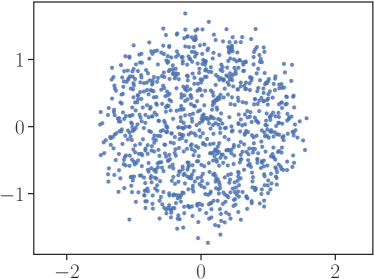
(a) $\beta_{n}=n^{3/2}$

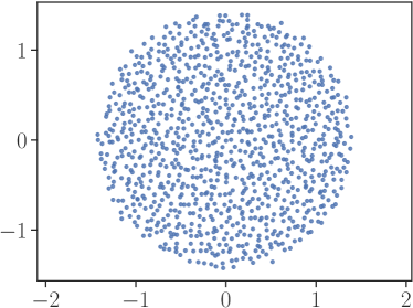
(b) $\beta_{n}=n^{2}$

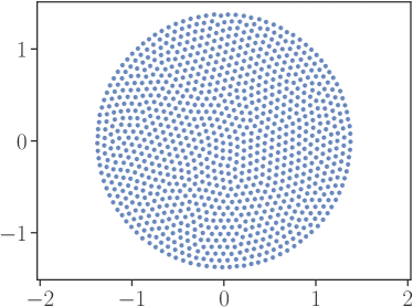
(c) $\beta_{n}=n^{3}$

Figure 1: Three independent approximate samples of $\mathbb{P}_{n,\beta_{n}}^{V}$ corresponding to different temperature schedules.

We first show how points sampled from $\mathbb{P}_{n,\beta_{n}}^{V}$ look like in dimension $d=2$, for the quadratic potential $V:x\mapsto\lvert x\rvert^{2}/2$, and for different scalings of the inverse temperature $\beta_{n}$. We consider the truncated logarithmic kernel $K(x,y)=-\log\left(\lvert x-y\rvert^{2}+\epsilon^{2}\right)$, where $\epsilon$ is a truncation parameter that we set to $\epsilon=10^{-2}$, and set the number of particles $n$ to $1000$. For $\epsilon=0$, the equilibrium measure is known to be uniform on the unit disk, and we expect it to be close to uniform in the truncated case as well. In each panel of Figure 1, we show the state of the MALA chain after $T=5000$ iterations, with step size $\alpha=\alpha_{0}\beta_{n}^{-1}$, and $\alpha_{0}$ is manually tuned at the beginning of each run so that acceptance reaches $50\%$.

We observe that the three empirical measures indeed approximate the uniform distribution on the disk, with more regular spacings as the inverse temperature grows. Figure 1b already shows a more regular arrangement of the points than under i.i.d. draws from the uniform distribution, while the lattice-like structure of Figure 1c is a manifestation of what physicists call crystallization (Serfaty, 2023): the Gibbs measure is concentrated around minimizers of the energy.

4.2 Comparing worst-case errors

In this experiment, we take for $\pi$ the uniform measure on the unit ball of $\mathbb{R}^{d}$, with $d=3$. We compare, for various values $n$ of the number of quadrature nodes, the worst-case integration error $I_{K}$ of $(i)$ the empirical measure $\mu_{n}^{\mathrm{MCMC}}$ of an MH chain of length $n$ targeting $\pi$, with an isotropic Gaussian proposal with variance $0.05I_{d}$, and of $(ii)$ the empirical measure $\mu_{n}$ of an approximate sample of $\mathbb{P}_{n,\beta_{n}}^{V}$. For the latter, we run MALA for $T=5\,000$ iterations, with step size tuned as in Section 4.1.

We consider two interaction kernels, the Gaussian kernel

$$K_{1}(x,y)=\exp\left(-\lvert x-y|^{2}/2\right)$$

and the truncated Riesz kernel

$$K_{2}(x,y)=\left(\lvert x-y\rvert^{2}+0.1^{2}\right)^{-(d-2)/2}.$$

For $K\in\{K_{1},K_{2}\}$, we set $V$ to $V^{\pi}$ as in Proposition 3.7, with $U_{K}^{\pi}(\cdot)$ replaced by a Monte Carlo approximation $M^{-1}\sum_{i=1}^{M}K(\cdot,z_{i})$, where $(z_{1},\dots,z_{M})$ are a sample from an MH chain of length $M=1\,000$ targeting $\pi$, independent from any other sample. This approximation is usual in kernel herding experiments (Pronzato & Zhigljavsky, 2020).

Figure 2b and 2a show the results for $K_{1}$ and $K_{2}$, respectively. For each value of $n$, we plot an independent approximation of $I_{K}(\mu-\pi)$ for $\mu\in\{\mu_{n}^{\mathrm{MCMC}},\mu_{n}\}$ the empirical measure of either the baseline MH chain or of the $T$-th iterate of our MALA chain targeting $\mathbb{P}_{n,\beta_{n}}^{V}$. The approximation results from writing

$$I_{K}(\mu-\pi)=I_{K}(\mu)-2I_{K}(\mu,\pi)+I_{K}(\pi),$$ (17)

in which the first term of (17) can be computed exactly when $\mu$ has finite support, but the other terms require independent MH samples targeting $\pi$, here of length $10,000$.

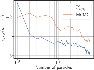
(a) Energy for the Gaussian kernel

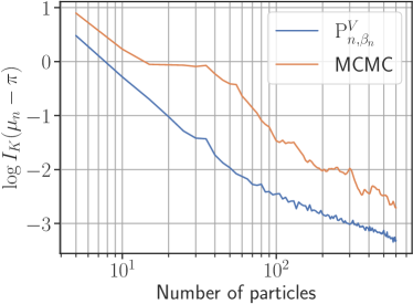
(b) Energy for the truncated Riesz kernel

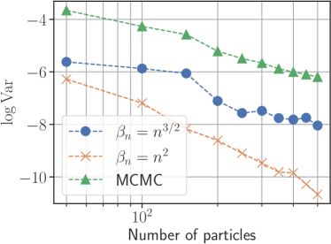
(c) Variance for the truncated Riesz kernel

Figure 2: Energy and variance comparisons between approximate samples from $\mathbb{P}_{n,\beta_{n}}^{V}$ and MCMC samples.

We observe that $I_{K}(\cdot-\pi)$ decays at the same rate under the approximation of $\mathbb{P}_{n,\beta_{n}}^{V}$ as for MCMC samples. This was expected, since our concentration bound (3.6) recovers the $n^{-1}$ rate for the energy $I_{K}(\mu_{n}-\pi)$ under $\mathbb{P}_{n,\beta_{n}}^{V}$, the improvement rather being on the sub-Gaussian decay. We see nonetheless that the approximated energy (and hence, the worst-case integration error) is always smaller by about a factor $3$ under $\mathbb{P}_{n,\beta_{n}}^{V}$, which is also expected since $\mathbb{P}_{n,\beta_{n}}^{V}$ favors small values of $I_{K}$ by definition.

4.3 Comparing variances for a single integrand

We know from classical CLT arguments that when $x_{1},\dots,x_{n}$ are drawn from an MCMC chain targeting $\pi$, the variance of $n^{-1}\sum_{i=1}^{n}f(x_{i})$ scales like $n^{-1}$ as $n$ grows, under appropriate assumptions on $f$. While this is not at all implied by our Corollary 3.6, analogies with the statistical physics literature make us expect a CLT to hold for $\mathbb{P}_{n,\beta_{n}}^{V}$, at rate ${\beta_{n}}^{-1/2}$, at least for some temperature schedules $(\beta_{n})$ and smooth enough integrands. Such a result would imply asymptotic confidence intervals for single integrands of width decreasing like $\beta_{n}^{-1/2}$, a faster decay than standard Monte Carlo. To assess whether this expectation is reasonable, we consider the same setting as in Section 4.2: $\pi$ is uniform on the unit ball in $d=3$, the kernel is the truncated Riesz kernel $K_{2}$, and the integrand is $f:x\longrightarrow K(x,0)$, which naturally belongs to $\mathcal{H}_{K}$. For each value of $n$ in Figure 2c, we run $100$ independent MH chains of length $n$ targeting $\pi$, and plot the empirical variance of the Monte Carlo estimator of $\int f\mathrm{d}\pi$. Similarly, we run $100$ independent MALA chains targeting $\mathbb{P}_{n,\beta_{n}}^{V}$ with $\alpha$ tuned as in Section 4.2, for $T=5000$ iterations each, and plot the $100$ empirical variances obtained from each $T$-th sample. Again, $U_{K_{2}}^{\pi}$ is approximated through long MH chains.

We observe in Figure 2c that the variance is noticeably smaller under the Gibbs measure, for both temperature schedules. Moreover, the rate of decay appears faster, at least in the “usual” temperature schedule $\beta_{n}=n^{2}$. It is hard to be more quantitative, as the fact we use MALA, and with a fixed number of iterations across all values of $n$, may impact the convergence we see here. Still, the experiment supports our belief that a fast CLT holds for $\mathbb{P}_{n,\beta_{n}}^{V}$.

5 Discussion

Using a Gibbs measure that favors nodes that repel according to a kernel $K$, we improved on the non-asymptotic worst-case integration guarantees of crude Monte Carlo, through a concentration inequality with a fairly easy proof, at least compared to the classical results in statistical physics that inspired us. When the RKHS of $K$ is infinite-dimensional, such an improvement has yet to be proved for deterministic IPM minimization. A strong argument in favor of a Gibbs measure would be a CLT with a fast rate. We show experimental evidence that supports this expectation.

Limitations of our approach that deserve further inquiry are the impact of using an approximation of the kernel embedding $U_{K}^{\pi}$ and an MCMC sampler, here MALA. Integrating a tractable approximation of $U_{K}^{\pi}$ without loss on the convergence speed would be an important improvement. Simultaneously, understanding how the accuracy of the MALA approximation relates to $n$ and $\beta_{n}$ would help find the right trade-off between statistical accuracy and computational cost.

Finally, compared to the bound (5) for volume sampling, our concentration bound features $\beta_{n}$, but not the eigenvalues of the kernel operator. In that sense, our confidence intervals are likely to be looser in an RKHS with fast-decaying kernel eigenvalues. Yet, establishing a CLT for the estimator in (5), where the weights in the estimator depend on all quadrature nodes, promises to be particularly hard. Moreover, if both distributions are approximately sampled through MCMC, one evaluation of our Gibbs density is quadratic in $n$, while it is cubic for volume sampling. A careful experimental comparison at fixed budget would thus be interesting.

Acknowledgments

We acknowledge support from ERC grant Blackjack ERC-2019-STG-851866, ANR grant Baccarat ANR-20-CHIA-0002 and Labex CEMPI (ANR-11-LABX-0007-01).

Appendix A Proofs

A.1 Proof of Proposition 3.3

The proof is a simple application of known results.

1. This is a consequence of the first point of Theorem $1.1$ in (Chafaï et al., 2014);

2. This is given by the second point of Lemma $2.2$ in (Chafaï et al., 2014);

3. This is a consequence of the ISDP assumption on the kernel, using Lemma $3.1$ in (Pronzato & Zhigljavsky, 2020). To see that $\mathcal{E}_{K}^{V}$ is non-empty, we can simply consider Dirac measures $\delta_{x}$, since $K$ is bounded and $V$ is finite everywhere.

4. This is a consequence of points $1$ and $3$ using the arguments of Section $4.1$ of (Chafaï et al., 2014).

A.2 Proof of Proposition 3.7

The proof of Proposition 3.7 relies on the so-called Euler-Lagrange equations, which we recall here.

Lemma A.1.

Let $K$ be a kernel satisfying Assumptions 1 and 2, and $V$ be an external potential satisfying 3. Set $C_{V}=I_{K}(\mu_{V})+\int V\,\mathrm{d}\mu_{V}$. Then $\mu_{V}$ has compact support, and a probability measure $\nu$ satisfies $\nu=\mu_{V}$ if and only if $\nu$ has compact support and there exists a constant $C$ such that

• $U_{K}^{\nu}(z)+V(z)\geq C$ for all $z\in\mathbb{R}^{d}$;

• $U_{K}^{\nu}(z)+V(z)\leq C$ for all $z\in supp(\nu)$.

In that case, $C=C_{V}$.

Proof.

Let us first check that $\mu_{V}$ satisfies this characterization. We already know from Proposition 3.3 that $\mu_{V}$ exists, is unique, and has compact support. We can use the same procedure as (Chafaï et al., 2014, Theorem $1.2$, proof of item $5$) : considering the directional derivative of $I_{K}^{V}$ and using the fact that $\mu_{V}$ is the minimizer, their equation ($4.5$) yields that, for any probability distribution $\nu\in\mathcal{E}_{K}^{V}$,

$$\int\left(V+U_{K}^{\mu_{V}}-C_{V}\right)\,\mathrm{d}\nu\geq 0.$$

Since Dirac measures $\delta_{z}$ have finite interaction energy $I_{K}^{V}(\delta_{z})$, we get Point $(i)$ by taking $\nu=\delta_{z}$. The second point is obtained exactly as in the second part of the proof of item $5$ of Theorem $1.2$ of Chafaï et al. (2014). Finally, the converse implication can be similarly obtained along the lines of the proof of item $6$ of Theorem $1.2$ in (Chafaï et al., 2014), using the strict convexity of the energy functional in Proposition 3.3. ∎

We are now ready to prove Proposition 3.7, by checking that the Euler-Lagrange equations are satisfied for $\pi$ and $V^{\pi}$, and that $V^{\pi}$ satisfies the assumptions of Proposition 3.3.

First note that since the kernel $K$ is nonnegative and bounded on the diagonal by assumption, Cauchy-Schwarz in the RKHS $\mathcal{H}_{K}$ implies that $K(x,y)\leq C$ for all $x,y\in\mathbb{R}^{d}$. As a consequence, since $K$ is further assumed to be continuous, Lebesgue’s dominated convergence theorem yields that $z\longmapsto U_{K}^{\pi}(z)$ is finite everywhere and continuous. In particular, $V^{\pi}$ is continuous.

Moreover, the bound on $K$ induces $0\leq U_{K}^{\pi}(z)\leq C$ for any $z\in\mathbb{R}^{d}$, so that $V^{\pi}(z)\longrightarrow+\infty$ when $\lvert z\rvert\longrightarrow+\infty$. Finally, the integrability assumption of 3 is satisfied by our assumption on $\Phi$ and because $U_{K}^{\pi}$ is bounded. Hence, $V^{\pi}$ satisfies 3 and the equilibrium measure $\mu_{V^{\pi}}$ is well-defined. We conclude upon noting that, since $\Phi\geq 0$, Lemma A.1 yields that $\mu_{V^{\pi}}=\pi$.

A.3 Proof of Theorem 3.5

The proof will follow the one of (Chafaï et al., 2018), with some notable simplifications. We first compute a lower bound on the partition function $Z_{n,\beta_{n}}^{V}$, which generalizes the one of (Chafaï et al., 2018) to bounded kernels.

Proposition A.2.

Let $K$ be a kernel satisfying Assumptions 1 and 2, and $V$ be an external potential satisfying 3. Assume that the associated equilibrium measure $\mu_{V}$ has finite entropy, i.e. $S(\mu_{V})=-\int\log\mu^{\prime}_{V}\mathrm{d}\mu_{V}<\infty$, where $\mu_{V}^{\prime}$ is the density of $\mu_{V}$ w.r.t. the Lebesgue measure. Then for $n\geq 2$, we have

$$Z_{n,\beta_{n}}^{V}\geq\exp\left\{-\beta_{n}I_{K}^{V}(\mu_{V})+n\left(\frac{\beta_{n}}{2n^{2}}I_{K}(\mu_{V})+S(\mu_{V})\right)\right\}.$$

Proof.

The idea is to rephrase a bit the discrete energy $H_{n}$ and use Jensen’s inequality.

We let $X_{n}=(x_{1},\dots,x_{n})$ for brevity, and we start by writing

$$n^{2}H_{n}(X_{n})=\frac{1}{2}\sum_{i\neq j}\{K(x_{i},x_{j})+V(x_{i})+V(x_{j})\}+\sum_{i=1}^{n}V(x_{i}).$$

Then

$$\log Z_{n,\beta_{n}}^{V}=\log\int_{\left(\mathbb{R}^{d}\right)^{n}}\exp\left(-\beta_{n}H_{n}(X_{n})\right)\mathrm{d}x_{1}\dots\,\mathrm{d}x_{n}$$

$$\geq\log\int_{E_{V}^{n}}\exp\left(-\frac{\beta_{n}}{2n^{2}}\sum_{i\neq j}\{K(x_{i},x_{j})+V(x_{i})+V(x_{j})\}-\sum_{i=1}^{n}\left(\frac{\beta_{n}}{n^{2}}V(x_{i})+\log\mu^{\prime}_{V}(x_{i})\right)\right)\mathrm{d}\mu_{V}(x_{1})\,\makebox[9.00002pt][c]{.\hfil.\hfil.\hfil}\,\mathrm{d}\mu_{V}(x_{n}),$$

where $E_{V}^{n}=\{(x_{1},\dots,x_{n})\in(\mathbb{R}^{d})^{n}:\prod_{i=1}^{n}\mu^{\prime}_{V}(x_{i})>0\}$. Using Jensen’s inequality, we get

$$\log Z_{n,\beta_{n}}^{V} \geq-\frac{\beta_{n}}{n^{2}}\sum_{i\neq j}\frac{1}{2}\int_{E_{V}^{n}}\left(K(x_{i},x_{j})+V(x_{i})+V(x_{j})\right)\mathrm{d}\mu_{V}(x_{1})\,\makebox[9.00002pt][c]{.\hfil.\hfil.\hfil}\,\mathrm{d}\mu_{V}(x_{n})$$

$$\quad-\sum_{i=1}^{n}\int_{E_{V}^{n}}\left(\frac{\beta_{n}}{n^{2}}V(x_{i})+\log\mu^{\prime}_{V}(x_{i})\right)\mathrm{d}\mu_{V}(x_{1})\,\makebox[9.00002pt][c]{.\hfil.\hfil.\hfil}\,\mathrm{d}\mu_{V}(x_{n})$$

$$=-\frac{\beta_{n}}{n^{2}}n(n-1)I_{K}^{V}(\mu_{V})-\frac{\beta_{n}}{n}\int V\mathrm{d}\mu_{V}+nS(\mu_{V}).$$

Using the definition $I_{K}^{V}(\mu_{V})=\frac{1}{2}I_{K}(\mu_{V})+\int V\mathrm{d}\mu_{V}$ we get the result. ∎

To bound $I_{K}(\mu_{n}-\mu_{V})$, we shall further use the following lemma, which is again inspired by (Chafaï et al., 2018).

Lemma A.3.

Let $K$ and $V$ be a kernel and an external potential satisfying Assumptions 1 to 3. Let $\mu$ be any probability measure of finite energy, $I_{K}^{V}(\mu)<+\infty$. Then

$$I_{K}(\mu-\mu_{V})\leq 2\left(I_{K}^{V}(\mu)-I_{K}^{V}(\mu_{V})\right).$$

Proof.

We write

$$I_{K}(\mu-\mu_{V})=\iint K(x,y)\,\mathrm{d}(\mu-\mu_{V})^{\otimes 2}=I_{K}(\mu)-2I_{K}(\mu,\mu_{V})+I_{K}(\mu_{V}).$$ (18)

With the notation of Lemma A.1, we know that $U_{K}^{\mu_{V}}(z)+V(z)=C_{V}$ for all $z$ in the support of $\mu_{V}$, and that $U_{K}^{\mu_{V}}(z)+V(z)\geq C_{V}$ in general. Using Fubini, we thus see that

$$I_{K}(\mu,\mu_{V})+\int V\,\mathrm{d}\mu =\int\left\{U_{K}^{\mu_{V}}(z)+V(z)\right\}\,\mathrm{d}\mu(z)$$

$$\geq C_{V}=I_{K}(\mu_{V})+\int V\,\mathrm{d}\mu_{V}.$$

Plugging this into (18) yields the result. ∎

We are now ready to prove Theorem 3.5. Recall that we work under the assumption $\beta_{n}\geq 2cn$ where $c$ is the constant of 3. Consider a Borel set $A\subset\left(\mathbb{R}^{d}\right)^{n}$. For brevity, recall that for $(x_{k})_{k\leq n}\in A$, we write $\mu_{n}=\frac{1}{n}\sum_{i=1}^{n}\delta_{x_{i}}$ and $X_{n}=(x_{1},\dots,x_{n})$.

Let $\eta>0$ and $X_{n}\in A$. The key idea is to split $H_{n}(X_{n})=(1-\eta)H_{n}(X_{n})+\eta H_{n}(X_{n})$. The first part will be compared with the energy $I_{K}^{V}(\mu_{n})$, while the second part will be kept to ensure integrability. Remembering that

$$n^{2}H_{n}(X_{n})=n^{2}I_{K}^{V}(\mu_{n})-\frac{1}{2}\sum_{i=1}^{n}K(x_{i},x_{i}),$$

we write, by definition,

$$\mathbb{P}_{n,\beta_{n}}^{V}(A) =\frac{1}{Z_{n,\beta_{n}}^{V}}\int_{A}\exp\left(-\beta_{n}H_{n}(X_{n})\right)\,\mathrm{d}x_{1}\,\dots\,\mathrm{d}x_{n}$$ (19)

$$=\frac{1}{Z_{n,\beta_{n}}^{V}}\exp\left(-\beta_{n}(1-\eta)I_{K}^{V}(\mu_{V})\right)\int_{A}\exp\left(-\beta_{n}(1-\eta)\left(I_{K}^{V}(\mu_{n})-I_{K}^{V}(\mu_{V})\right)\right)$$

$$\quad\times\exp\left(\frac{\beta_{n}}{2n^{2}}(1-\eta)\sum_{i=1}^{n}K(x_{i},x_{i})-\beta_{n}\eta H_{n}(X_{n})\right)\,\mathrm{d}x_{1}\,\makebox[9.00002pt][c]{.\hfil.\hfil.\hfil}\,\mathrm{d}x_{n}.$$ (20)

Using Proposition A.2, we continue

$$\mathbb{P}_{n,\beta_{n}}^{V}(A) \leq\exp\left(-n\left(S(\mu_{V})+\frac{\beta_{n}}{2n^{2}}I_{K}(\mu_{V})\right)+\beta_{n}\eta I_{K}^{V}(\mu_{V})\right)$$ (21)

$$\quad\times\exp\left(-\beta_{n}(1-\eta)\underset{A}{\,\inf}\left(I_{K}^{V}(\mu_{n})-I_{K}^{V}(\mu_{V})\right)\right)$$ (22)

$$\quad\times\int_{\mathbb{R}^{d}}\exp\left(\frac{\beta_{n}}{2n^{2}}(1-\eta)\sum_{i=1}^{n}K(x_{i},x_{i})-\beta_{n}\eta H_{n}(X_{n})\right)\,\mathrm{d}x_{1}\,\makebox[9.00002pt][c]{.\hfil.\hfil.\hfil}\,\mathrm{d}x_{n}.$$ (23)

As noted in the proof of Lemma A.1, $0\leq K\leq C$, so that the last integral in (23) is easily bounded,

$$\int_{\mathbb{R}^{d}}\exp\left(\frac{\beta_{n}}{2n^{2}}(1-\eta)\sum_{i=1}^{n}K(x_{i},x_{i})-\beta_{n}\eta H_{n}(X_{n})\right)\,\mathrm{d}x_{1}\,\dots\,\mathrm{d}x_{n}$$

$$\quad\leq\exp\left(\frac{\beta_{n}}{2n}(1-\eta)C\right)\left(\int_{\mathbb{R}^{d}}\exp\left(-\frac{\beta_{n}}{n}\eta V(x)\right)\,\mathrm{d}x\right)^{n}.$$

Now we choose a particular value for $\eta$, namely $\eta=cn/\beta_{n}$ where $c$ is the constant of 3. Further let $C_{2}=\log\int_{\mathbb{R}^{d}}\exp\left(-cV(x)\right)\,\mathrm{d}x$, which is finite by assumption. Setting $c_{1}=cI_{K}^{V}(\mu_{V})+C_{2}-S(\mu_{V})$ and $c_{2}=\frac{1}{2}C-\frac{1}{2}I_{K}(\mu_{V})$, (23) yields

$$\mathbb{P}_{n,\beta_{n}}^{V}\left(A\right)\leq\exp\left(-(\beta_{n}-cn)\underset{A}{\,\inf}\left(I_{K}^{V}(\mu_{n})-I_{K}^{V}(\mu_{V})\right)+nc_{1}+\frac{\beta_{n}}{n}c_{2}\right).$$ (24)

Note that $c_{1}$ and $c_{2}$ are indeed finite by definition of $\mu_{V}$, since $\mathcal{E}_{K}^{V}$ is non-empty. The comparison inequality of Lemma A.3 applied to (24), with

$$A=\{I_{K}(\mu_{n}-\mu_{V})>r^{2};\mu_{n}=\frac{1}{n}\sum_{i=1}^{n}\delta_{x_{i}}\},$$

yields Theorem 3.5, upon noting that $\beta_{n}-cn\geq\beta_{n}/2$ by assumption.

References

- Alquier et al. (2016) Alquier, P., Ridgway, J., and Chopin, N. On the properties of variational approximations of Gibbs posteriors. The Journal of Machine Learning Research, 17(1):8374–8414, 2016.
- Anastasiou et al. (2023) Anastasiou, A., Barp, A., Briol, F.-X., Ebner, B., Gaunt, R. E., Ghaderinezhad, F., Gorham, J., Gretton, A., Ley, C., Liu, Q., Mackey, L., Oates, C. J., Reinert, G., and Swan, Y. Stein’s Method Meets Computational Statistics: A Review of Some Recent Developments. Statistical Science, 38(1):120 – 139, 2023. doi: 10.1214/22-STS863.
- Bach (2017) Bach, F. On the equivalence between kernel quadrature rules and random feature expansions. The Journal of Machine Learning Research, 18(1):714–751, 2017.
- Bach et al. (2012) Bach, F., Lacoste-Julien, S., and Obozinski, G. On the Equivalence between Herding and Conditional Gradient Algorithms. In Proceedings of the 29th International Coference on International Conference on Machine Learning, ICML’12, pp. 1355–1362, Madison, WI, USA, 2012. Omnipress. ISBN 9781450312851.
- Bauerschmidt et al. (2016) Bauerschmidt, R., Bourgade, P., Nikula, M., and Yau, H.-T. The two-dimensional Coulomb plasma: quasi-free approximation and central limit theorem. arXiv preprint arXiv:1609.08582, 2016.
- Belhadji et al. (2020) Belhadji, A., Bardenet, R., and Chainais, P. Kernel interpolation with continuous volume sampling. In International Conference on Machine Learning (ICML), 2020.
- Berlinet & Thomas-Agnan (2011) Berlinet, A. and Thomas-Agnan, C. Reproducing kernel Hilbert spaces in probability and statistics. Springer Science & Business Media, 2011.
- Blei et al. (2017) Blei, D. M., Kucukelbir, A., and McAuliffe, J. D. Variational inference: A review for statisticians. Journal of the American statistical Association, 112(518):859–877, 2017.
- Bolley et al. (2007) Bolley, F., Guillin, A., and Villani, C. Quantitative concentration inequalities for empirical measures on non-compact spaces. Probability Theory and Related Fields, 137:541–593, 2007.
- Chafaï et al. (2014) Chafaï, D., Gozlan, N., and Zitt, P.-A. First-order global asymptotics for confined particles with singular pair repulsion. Ann. Appl. Probab., 24(6):2371–2413, 2014. ISSN 1050-5164. doi: 10.1214/13-AAP980.
- Chafaï et al. (2018) Chafaï, D., Hardy, A., and Maïda, M. Concentration for Coulomb gases and Coulomb transport inequalities. J. Funct. Anal., 275(6):1447–1483, 2018. ISSN 0022-1236. doi: 10.1016/j.jfa.2018.06.004.
- Chafaï & Ferré (2018) Chafaï, D. and Ferré, G. Simulating Coulomb gases and log-gases with hybrid Monte Carlo algorithms. 06 2018.
- Chen & Welling (2010) Chen, Y. and Welling, M. Parametric Herding. In Teh, Y. W. and Titterington, M. (eds.), Proceedings of the Thirteenth International Conference on Artificial Intelligence and Statistics, volume 9 of Proceedings of Machine Learning Research, pp. 97–104, Chia Laguna Resort, Sardinia, Italy, 13–15 May 2010. PMLR.
- Chen et al. (2010) Chen, Y., Welling, M., and Smola, A. Super-Samples from Kernel Herding. In Proceedings of the Twenty-Sixth Conference on Uncertainty in Artificial Intelligence, UAI’10, pp. 109–116, Arlington, Virginia, USA, 2010. AUAI Press. ISBN 9780974903965.
- Dembo & Zeitouni (2009) Dembo, A. and Zeitouni, O. Large deviations techniques and applications, volume 38. Springer Science & Business Media, 2009.
- Dick et al. (2013) Dick, J., Kuo, F. Y., and Sloan, I. H. High-dimensional integration: the quasi-Monte Carlo way. Acta Numerica, 22:133–288, 2013.
- Fournier & Guillin (2015) Fournier, N. and Guillin, A. On the rate of convergence in Wasserstein distance of the empirical measure. Probability theory and related fields, 162(3-4):707–738, 2015.
- García-Zelada & Padilla-Garza (2022) García-Zelada, D. and Padilla-Garza, D. Generalized transport inequalities and concentration bounds for Riesz-type gases. arXiv preprint arXiv:2209.00587, 2022.
- Hoffman et al. (2013) Hoffman, M. D., Blei, D. M., Wang, C., and Paisley, J. Stochastic variational inference. Journal of Machine Learning Research, 2013.
- Korba et al. (2020) Korba, A., Salim, A., Arbel, M., Luise, G., and Gretton, A. A non-asymptotic analysis for Stein variational gradient descent. Advances in Neural Information Processing Systems, 33:4672–4682, 2020.
- Korba et al. (2021) Korba, A., Aubin-Frankowski, P.-C., Majewski, S., and Ablin, P. Kernel stein discrepancy descent. In International Conference on Machine Learning, pp. 5719–5730. PMLR, 2021.
- Lambert et al. (2022) Lambert, M., Chewi, S., Bach, F., Bonnabel, S., and Rigollet, P. Variational inference via Wasserstein gradient flows. Advances in Neural Information Processing Systems, 35:14434–14447, 2022.
- Leblé & Serfaty (2018) Leblé, T. and Serfaty, S. Fluctuations of two dimensional Coulomb gases. Geometric and Functional Analysis, 28:443–508, 2018.
- Liu & Wang (2016) Liu, Q. and Wang, D. Stein variational gradient descent: A general purpose bayesian inference algorithm. Advances in neural information processing systems, 29, 2016.
- Murphy (2023) Murphy, K. P. Probabilistic machine learning: Advanced topics. MIT press, 2023.
- Pronzato (2023) Pronzato, L. Performance analysis of greedy algorithms for minimising a Maximum Mean Discrepancy. Statistics and Computing, 33(1):14, 2023.
- Pronzato & Zhigljavsky (2020) Pronzato, L. and Zhigljavsky, A. Bayesian quadrature, energy minimization, and space-filling design. SIAM/ASA Journal on Uncertainty Quantification, 8(3):959–1011, 2020.
- Rasmussen & Williams (2006) Rasmussen, C. and Williams, C. Gaussian Processes for Machine Learning. Adaptive Computation and Machine Learning. MIT Press, Cambridge, MA, USA, January 2006.
- Robert (2007) Robert, C. P. The Bayesian choice: from decision-theoretic foundations to computational implementation. Springer Science & Business Media, 2007.
- Robert & Casella (2004) Robert, C. P. and Casella, G. Monte Carlo statistical methods. Springer Texts in Statistics. Springer-Verlag, New York, second edition, 2004. ISBN 0-387-21239-6. doi: 10.1007/978-1-4757-4145-2.
- Serfaty (2018) Serfaty, S. Systems with Coulomb interaction. Notices of the American Mathematical Society, 65(7):787–788, August 2018. ISSN 0002-9920. doi: 10.1090/noti1697.
- Serfaty (2023) Serfaty, S. Gaussian fluctuations and free energy expansion for Coulomb gases at any temperature. In Annales de l’Institut Henri Poincare (B) Probabilites et statistiques, volume 59, pp. 1074–1142. Institut Henri Poincaré, 2023.
- Sriperumbudur et al. (2010) Sriperumbudur, B. K., Gretton, A., Fukumizu, K., Schölkopf, B., and Lanckriet, G. R. G. Hilbert space embeddings and metrics on probability measures. J. Mach. Learn. Res., 11:1517–1561, 2010. ISSN 1532-4435.
- Welling (2009) Welling, M. Herding Dynamical Weights to Learn. In Proceedings of the 26th Annual International Conference on Machine Learning, ICML ’09, pp. 1121–1128, New York, NY, USA, 2009. Association for Computing Machinery. ISBN 9781605585161. doi: 10.1145/1553374.1553517.
- Welling (2012) Welling, M. Herding dynamic weights for partially observed random field models. arXiv preprint arXiv:1205.2605, 2012.