Prospector Heads:
Generalized Feature Attribution for Large Models & Data

Abstract

Feature attribution, the ability to localize regions of the input data that are relevant for classification, is an important capability for machine learning models in scientific and biomedical domains. Current methods for feature attribution, which rely on explaining the predictions of end-to-end classifiers, suffer from imprecise feature localization and are inadequate for use with small sample sizes and high-dimensional datasets due to computational challenges. We introduce prospector heads, an efficient and interpretable alternative to explanation-based methods for feature attribution that can be applied to any encoder and any data modality. Prospector heads generalize across modalities through experiments on sequences (text), images (pathology), and graphs (protein structures), outperforming baseline attribution methods by up to 49 points in mean localization AUPRC. We also demonstrate how prospector heads enable improved interpretation and discovery of class-specific patterns in the input data. Through their high performance, flexibility, and generalizability, prospectors provide a framework for improving trust and transparency for machine learning models in complex domains.

1 Introduction

Most machine learning models are optimized solely for predictive performance, but many applications also necessitate models that provide insight into features of the data that are unique to a particular class. This capability is known as feature attribution, which in unstructured data (e.g., text, images, graphs) consists of identifying subsets of the input datum (e.g., pixels or patches of an image, often represented as a heatmap) most responsible for that datum’s class membership. Feature attribution is especially important for scientific and biomedical applications. For example, for a model to assist a pathologist in making a cancer diagnosis, it ideally should not only accurately classify which images contain tumors, but also precisely locate the cancer cells in each image [59, 51].

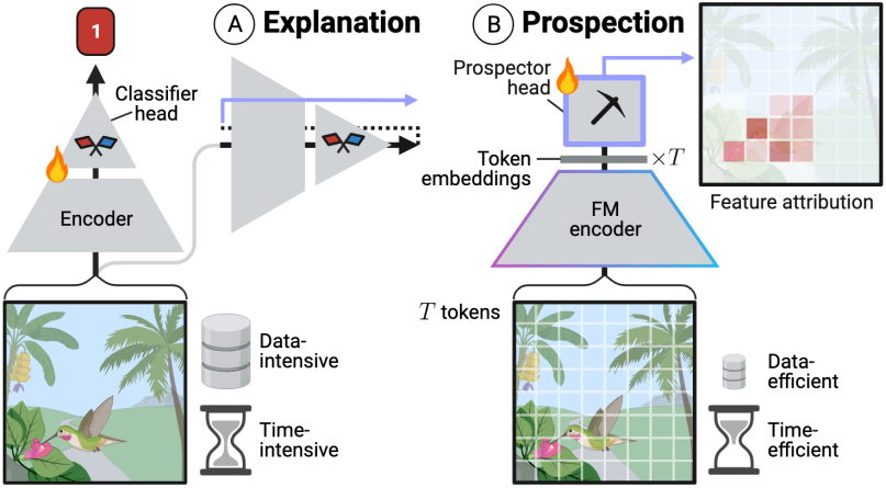
Figure 1: After training a classifier, explanation-based attribution uses either a model’s internal layers, gradients (dashed line), or input perturbations (A). These methods are limited by large amounts of training data and large time complexity. Our solution, the prospector head (B), is encoder-equippable like classifier heads and adapts embeddings. Flame icons indicate trainable parameters.

Unfortunately, modern AI systems struggle to perform feature attribution. Most existing attribution techniques attempt to provide an explanation (Figure 1) — either a description of how a trained classifier’s weights interact with different input features (e.g., gradients [58], attention [39]) or a description of each feature’s contribution to prediction (e.g., SHAP [48], LIME [55]). Explanation-based attribution methods (a) require a lot of labeled training data due to their reliance on underlying classifiers, but large datasets are often unavailable in biomedical applications. Additionally, the methods producing explanations can themselves be (b) computationally expensive [4, 18, 21] and thus may not actually improve tractability relative to annotation by domain experts, particularly for large inputs. Finally, (c) the attributed features are often found to be inaccurate and not actually relevant to the target classes [7, 70, 36, 72].

We explore whether foundation models (FMs) can be used to solve challenges (a–c) without traditional explanations. Prior work has demonstrated that FMs learn high quality data representations and can learn class-specific properties through a few labeled examples [11, 14, 30]. However, it is unclear whether FM representations can be used to perform feature attribution in a scalable and accurate manner. Our key insight is to build on top of FM representations, rather than explain an FM tuned as an end-to-end classifier.

In this work we present the prospector head, a simple decoder module that aims to equip feature attribution to any encoder — including FMs — just as we often equip classification heads. Prospector heads contain only two layers: layer (I) categorizes learned representations into a finite set of concepts and layer (II) learns concepts’ spatial associations and how those associations correlate with a target class. To (a) enable data efficiency, prospector heads are parameter-efficient and typically require only hundreds of parameters. To (b) limit time-complexity, prospector heads operate with efficient data structures, linear-time convolutions, and without model backpropagation. To (c) improve attribution accuracy, prospector heads are explicitly trained to perform feature attribution, unlike explanation methods.

We experimentally show prospector heads outperform baselines over multiple challenging data modalities. In terms of feature attribution performance, prospector-equipped models achieve gains in mean AUPRC of up to +43 points in sequences (text documents), +31 points in images (pathology slides), and +49 points in graphs (protein structures) over modality-specific baselines. Additionally, we show that FMs with attached prospector heads are particularly robust to differences in the prevalence and distribution of class-specific features. Finally, we also present visualizations of prospector heads’ parameters and outputs to demonstrate their interpretability in complex domain applications.

2 Related Work

2.1 Feature Attribution via Explanation

In the current explanation-based paradigm, feature attribution is done by (1) explicitly training a model to learn the mapping from each datum $X$ to its class label $X\mapsto y$ before (2) inferring class-specific features using one of the explainability approaches described below. This framework can be described as weak or coarse supervision [56] due to the use of only class label $y$ as a supervisory signal and the low signal-to-noise ratio in the $(X,y)$ pairs, particularly when the prevalence of class-specific features is low [52].

Model-specific methods like gradient-based saliency maps [58], class-activation maps (CAMs) [71, 57, 63], and attention maps [39] use a classifier’s internals (e.g., weights, layer outputs), inference, and/or backpropagation for attribution. Recent work has demonstrated gradients serve as poor localizers [7, 70] — potentially due to their unfaithfulness in reflecting classifiers’ reasoning processes [40] and propensity to identify spurious correlations despite classifier non-reliance [1]. Furthermore, CAMs pose high computational costs with multiple forward and backward passes [19]. Finally, attention maps are demonstrably poor localizers [72] also perhaps due to their unfaithfulness [66] and difficulties in assigning class membership to input features [36].

On the other hand, model-agnostic methods like SHAP [48] and LIME [55] perturb input features to determine their differential contribution to classification. Recent work [10] has shown SHAP struggles to localize class-specific regions and is provably no better than a random explainer with respect to each input feature. Furthermore, SHAP-style methods can be computationally expensive for a variety of reasons. Some methods face exponential or quadratic time complexities [4] with respect to the number of input features (e.g., pixels in an image) and are thus infeasible for high-dimensional data, while others require multiple forward and/or backward passes [18] or require training additional comparably sized deep networks along with the original classifier [38]. While LIME offers faithful explanations, and can even reveal a classifier’s reliance on spurious correlations, it can generate vastly different explanations for similar examples [2] and is also computationally costly due to training surrogate models per datum. Finally, concept-based feature attribution [29, 22] is a newer modality-generalizable family of methods that aligns machine- and human-derived concepts to construct a “shared vocabulary” by which to explain predictions.

2.2 Modern Encoders & Context Sizes

Most modern encoders for unstructured data operate on tokens, or relatively small pieces of a datum, creating intermediate representations that we can leverage to identify class-specific regions. Tokens are often prespecified by the user and/or constructed by the encoder itself — where these encoders are respectively referred to as partial-context and full-context (Figure 2). Determining encoder context is based on practical modeling constraints: computational complexity of an architecture’s modeling primitives, input data dimensionality, and hardware. For example, suppose we want to build an encoder for image data. We may choose to train a Transformer [61, 25], a predominant architecture that experiences quadratic time complexity [41] with respect to input dimension. Standard images (e.g., $224\times 224$ pixels) easily fit in modern GPU memory, enabling a full-context Transformer encoder to be trained. Such a model would create token embeddings via intermediary layers. However, gigapixel images require user-prespecified tokens (i.e., patches) and partial-context encoders that create an embedding for each prespecified token [47, 35, 43, 44].

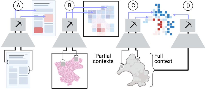
Figure 2: Prospector heads are modality-generalizable with support for sequences (A), images (B), and graphs (C,D). They can also operate on embeddings from either partial- or full-context encoders (C,D).

Gradient-based saliency and attention maps have been used to explain partial-context classifiers for high-dimensional unstructured data like gigapixel imagery [16, 20]. However, studies have reported low specificity and sensitivity [49] in part because attribution for the entire datum is often built by concatenating attributions across prespecified tokens (e.g., image patches). Such approaches assume prespecified tokens are independent and identically distributed (IID), which does not hold for unstructured data.

3 Methods

3.1 Preliminaries

In order to enable any FM to perform feature attribution regardless of input modality, we first construct a generalized language for unstructured data. Any unstructured datum can be represented by a map graph $G(\mathcal{V},\mathcal{E})$ where each vertex $v\in\mathcal{V}$ represents a discrete token, or piece of that datum in Euclidean space (Definition A.1). For example, in image data, tokens can be defined as pixels or patches. An edge $e_{i\leftrightarrow j}\in\mathcal{E}$ connects vertex $v_{i}$ to $v_{j}$. Both $G$’s token resolution and token connectivity are defined depending on data modality (Figure 8).

Problem setup: Suppose we have a dataset containing map graphs $G$ and binary class labels $y$. The multiple instance assumption (MIA) posits that class₁ graphs ($y=1$) largely resemble class₀ graphs ($y=0$) with the exception of vertices (i.e., tokens) only found in class₁ graphs [3, 28]. In other words, we assume that a class₁ graph $G(\mathcal{V},\mathcal{E})$ contains a set of class₁-specific vertices $\mathcal{V}_{y}\subseteq\mathcal{V}$, with $|\mathcal{V}_{y}|\geq 1$ [71]. The primary task of feature attribution is to locate all $\mathcal{V}_{y}$ in each datum given a set of $(G,y)$ pairs as a training dataset.

3.2 Prospection: Attribution sans Explanation

We now present prospector heads, a.k.a. prospectors, a simple decoder module built to perform few-shot feature attribution for high-dimensional data. This module is equippable to virtually any pre-trained encoder, including FMs. Prospectors use two layers to perform feature attribution. Crucially, prospectors interface with encoders by adapting their token embeddings, which serve as the unit of analysis. We underscore how this is at odds with explanation-based attribution, where datum-level embeddings are used. A key assumption is that equipped encoders have learned their distributional semantics in encoder pre-training. In layer (I), prospectors transform token embeddings into feature categories, or concepts, learned from the training set. Layer (II) then attributes scores to each token using graph convolution, based on concept frequencies and co-occurrences. The following sections describe how a prospector performs feature attribution at inference time, followed by fitting procedures for each layer.

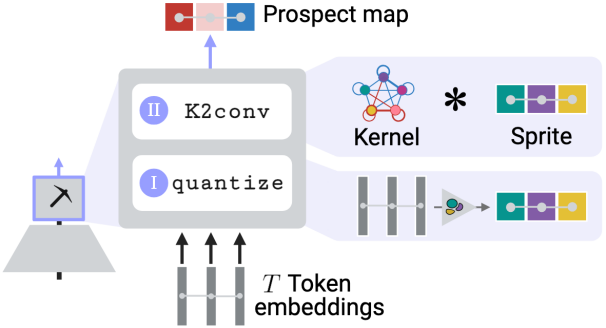
Figure 3: Prospector module applied to an input datum to produce a prospect map. Details for fitting layers (I) and (II) are in Section A.3.

3.2.1 Receiving Token Embeddings

Prospectors receive token embeddings $\mathbf{x}_{1}\ldots\mathbf{x}_{T}$ from an equipped encoder and update map graph $G$ such that each vertex $v_{i}\in\mathcal{V}$ is featurized by an embedding $\mathbf{x}_{i}\in\mathbb{R}^{d}$. This vertex-specific feature loading uses the notation: $G[v_{i}]:=\mathbf{x}_{i}$. Details for partial- and full-context encoders are specified in Section A.1.

3.2.2 Layer I: Quantizing Embeddings

Next, prospectors use an encoder’s learned semantics to construct a vocabulary of $k$ token concepts $\mathcal{C}={1,\ldots,k}$. This is achieved by quantizing (i.e., categorizing) each token embedding $\mathbf{x}\in\mathbb{R}^{d}$ as scalar concepts $c\in\mathcal{C}$:

$$c_{i}=\texttt{quantize}(\mathbf{x}_{i})\quad\forall i=1\ldots T.$$

When the quantize layer (Section 3.3.1) is applied over the full graph $G$, it is transformed into graph $S$ with the same topology as $G$, but with categorical vertex features $S[v_{i}]:=c_{i}\>\forall i$. We refer to $S$ as a data sprite due to its low feature dimensionality compared to $G$, with data compression ratio of $d$. Intuitively, the heterogeneity of $S$ is parameterized by the choice of $k$.

3.2.3 Layer II: Convolution over Concepts

Prospectors next perform feature attribution using a graph convolution over sprite $S$. Convolution requires a global kernel $\omega$ that computes an attribution score $a\in\mathbb{R}$ for each vertex $v$ based on the concepts $c_{i}$ (i.e., monograms) and co-occurrences $c_{i},c_{j}$ (i.e., skip-bigrams) present within the graph neighborhood defined by receptive field $r$. The kernel $\omega$ can be conceptualized as a dictionary, scoring each concept monogram or skip-bigram in the combinatorial space $\mathcal{Z}=\mathcal{C}\cup\{\mathcal{C}\otimes\mathcal{C}\}$, where $\otimes$ is the Cartesian product. The global kernel is fit over the training set (Section 3.3.2).

To perform feature attribution at inference time, we apply the fitted kernel over each vertex in a datum to produce a prospect map $P$. $P$ is a map graph with the same topology as $G$ and $S$ but featurized by scalar continuous attribution scores $P[v]:=a$. We call this layer K2conv in reference to kernel $\omega$’s implicit structure (Definition A.4). An attribution score $a_{i}$ is computed for each vertex $v_{i}$ in $S$, where $\mathcal{N}_{r}$ represents all vertices within the $r$-neighborhood of $v_{i}$ (including $v_{i}$ itself):

$$P[v_{i}]:=a_{i}=\overbrace{\mathcal{N}_{r}*\omega}^{\text{{K2conv} }}=\smashoperator[]{\sum_{\forall v_{j}\in\mathcal{N}_{r}}^{}}\omega\left<\overbrace{S[v_{j}]}^{c_{i}}\right>\>\>+\quad\>\smashoperator[]{\sum_{\forall(v_{j},v_{k})\in\mathcal{N}_{r}}^{}}\omega\left<(\overbrace{S[v_{j}]}^{c_{j}},\overbrace{S[v_{k}]}^{c_{k}})\right>,$$

where $\omega\langle\cdot\rangle$ denotes dictionary lookup. The resulting prospect map $P$ aims to capture the class-specific region $\mathcal{V}_{y}$ by assigning high absolute positive or negative values to each token. Intuitively, $r$ parameterizes the level of smoothing over $P$ by modulating the number of neighboring tokens used to compute a token’s importance. Further details for each layer and runtime analysis are found in Appendix A.

3.3 Fitting Prospector Layers

In our implementation, layers (I) and (II) are fitted separately and sequentially using the procedures below.

3.3.1 Fitting Layer I Quantizer

Prospectors learn $k$ semantic concepts in order to quantize token embeddings. Token embeddings from across the training set are partitioned into $k$ subspaces using a clustering method (e.g., $k$-means). After clustering, each subspace represents a semantic concept $c\in\mathcal{C}$ discovered in the corpus. To reduce computation, clustering can be performed over a representative sample ($>10^{3}$) of the token embedding space, randomly sampled without replacement. Fitting is depicted in Figure 9.

3.3.2 Fitting Layer II Kernel

Fitting the K2conv kernel involves computing the class-attribution weights for each monogram and skip-bigram in $\mathcal{Z}$ across the training set. These weights represent the only learnable parameters of a prospector head. The number of parameters $|\mathcal{Z}|$ is therefore dependent on $k$ and is at maximum (Section A.3.3): $|\mathcal{Z}|=2k+{k\choose 2}$. The kernel is fit in two steps, as outlined below.

Step 1: Computing frequencies & co-occurrences.

For each sprite $S$ in the training set, prospectors build a representation that counts and tracks all concept monograms and skip-bigrams within the $r$-neighborhood of each vertex. This is performed by the rollup operator:

$$\mathbf{z}=\texttt{rollup}(S).$$

Explicitly, the rollup operator traverses $S$’s vertices and sums the counts of each element $z_{i}\in\mathcal{Z}$ to form a vector $\mathbf{z}\in\mathbb{R}^{|\mathcal{Z}|}$, which we refer to as a sprite embedding. This vector is then normalized to account for differences in baseline frequencies (e.g., using TF-IDF [60]). The rollup operator and this step as a whole are described in Algorithm 1 and Figure 10.

Step 2: Learning kernel weights.

Prospectors next use the datum-level sprite embeddings $\mathbf{z}$ to learn a vector $\mathbf{w}\in\mathbb{R}^{|\mathcal{Z}|}$ of class-specific weights for each monogram and skip-bigram across the entire training set. After fitting $\mathbf{w}$, we construct $\omega$ as a dictionary mapping each element in $\mathcal{Z}$ to its corresponding weight in $\mathbf{w}$. We implement two approaches to learning weights, which make up the two main prospector variants: a linear classifier $h_{\mathbf{w}}$ and a parameter-free fold-change computation. These variants are discussed in Section A.4 and depicted graphically in Figure 10.

Linear classifier: This approach trains a linear classifier $h_{\mathbf{w}}(\mathbf{z})=\mathbf{w}^{\intercal}\mathbf{z}$ to learn a mapping from $\mathbf{z}\mapsto y$ over the training dataset. The learned coefficients $\mathbf{w}$ then represent the class-specific importance of each index in $\mathbf{z}$. We implement this as a logistic regression with elastic net regularization with the mixing hyperparameter $\lambda$.

Fold-change computation: This approach involves first computing mean sprite embeddings for each class over the training data. For example, for the negative class, $\overline{\mathbf{z}}_{0}=\frac{1}{|\mathcal{D}_{0}|}\sum_{S^{(i)}\in\mathcal{D}_{0}}{\mathbf{z}^{(i)}}$, where $\mathcal{D}_{0}$ is the subset of the training dataset $(S^{(i)},y^{(i)})$ for which $y^{(i)}=0$. Then, we compute $\mathbf{w}$ as a fold-changes $\mathbf{w}=\operatorname{log}_{2}(\overline{\mathbf{z}}_{1})-\operatorname{log}_{2}(\overline{\mathbf{z}}_{0})$ and select significant weights using a hypothesis test for the difference of independent means [5].

3.4 Guiding Design Principles

Prospectors overcome the limitations of current feature attribution methods by observing the following design principles. Firstly, in order to operate in few-shot settings, prospectors are (a) parameter efficient due to the use of concept monograms and skip-bigrams alone to build its kernel. Both methods for computing feature attribution scores are also data efficient — linear models at maximum use only $2k+{k\choose 2}$ parameters, while hypothesis testing is entirely parameter-free. Secondly, prospectors are (b) computationally efficient: by operating as an equippable head, prospectors are plug-in-ready without encoder retraining [42] and or backpropagation. In combination with the use of efficient modeling primitives such as learnable dictionaries and convolution (linear-time with respect to the tunable number of tokens $T=|\mathcal{V}|$), this allows prospectors to efficiently scale feature attribution to high-dimensional data. Finally, prospectors achieve (c) improved localization and class-relevance by prospectors explicitly train on token embeddings to learn $G_{y}$ instead of using end-to-end classifiers to identify $G_{y}$ post hoc.

4 Experiments

4.1 Datasets, Encoders, & Baselines

We evaluate prospectors using three primary tasks, each representing a different data modality (sequences, images, and graphs). Each also poses unique challenges for prospector training and feature attribution: class imbalance (sequences), high input dimensionality with few examples (images), and very coarse supervision (graphs). Details for each dataset’s construction are shared in Section B.4. For each task, we select a representative set of encoders to which we equip prospector heads and note whether the encoder operates on the level of full context (i.e., entire datum) or partial context (i.e., prespecified tokens). For each encoder, we compare prospector heads to relevant and computationally feasible baseline methods. We summarize encoders in Table 1 and describe baselines in Section B.6.

Encoder Alias	Architecture	Learning Regime	Training Epochs	Embed Size ($d$)
MiniLM	MiniLM-L6	KD	✗	384
tile2vec	ResNet-18	USL	20	128
ViT	ViT/16	WSL	30	1024
CLIP	ViT-B/32	SSL	✗	512
PLIP	ViT-B/32	SSL	✗	512
COLLAPSE	GVP-GNN	SSL	✗	512
ESM2	t33_650M_UR50D	SSL	✗	1028
AA	N/A	N/A	✗	21

Table 1: Prospector-equipped encoders in descending order by modality: sequences, images, and graphs. Learning regimes are knowledge distillation (KD), unsupervised learning (USL), weakly supervised learning (WSL), and self-supervised learning (SSL). Pre-training denoted by ✗.

For both baselines and prospectors, we perform a gridsearch over tunable hyperparameters. The best models were selected based on their ability to localize ground truth class-specific regions in the training set, since these were not seen by the models during training. We use a sequential ranking criteria over four token-level metrics: precision, dice coefficient, Matthews correlation coefficient, and AUPRC. Details of hyperparameter tuning and model selection are found in Section B.1 and B.2. The results in the remainder of this paper present the localization AUPRC for class-specific regions in our held-out test data.

Sequences: key sentence retrieval in text documents.

Retrieval is an important task in language modeling that provides in-text answers to user queries. For this task, we use the WikiSection [6] benchmark dataset created for paragraph-level classification. We repurpose WikiSection to assess the ability to retrieve target sentences specific to a queried class. We specifically use the genetics section label as a query, and class₁ data are defined as documents in the English-language disease subset that contain this section label. Our goal is to identify sentences that contain genetics-related information given only coarse supervision from document-level labels. After preprocessing the pre-split dataset, our dataset contained 2513 training examples (2177 in class₀, 336 in class₁) and 712 test examples. The relationship between sentences in each document is represented as a graph with 2-hop connectivity (Figure 8).

Encoders & baselines: We apply prospector heads to a MiniLM-L6 [64] encoder, a popular language model pretrained on sentences and small paragraphs to naturally reflect partial contexts in text documents. Since there are few explanation-based feature attribution methods for text, we compare prospectors to other supervised heads which are trained to predict class-specific labels for each token individually. Specifically, we compare to a multi-layer perception (MLP) trained on labeled token embeddings and a one-class support vector machine (SVM) trained solely on class₀ token embeddings. In the latter case, we perform novelty detection to identify class₁ embeddings.

Images: tumor localization in pathology slides.

Identifying tumors is an important task in clinical pathology, where manual annotation is standard practice. We evaluate prospectors on Camelyon16 [26], a benchmark of gigapixel pathology images, each presenting either healthy tissue or cancer metastases. All images are partitioned into prespecified $224\times 224$ patch tokens and filtered for foreground tissue regions. After pre-processing the pre-split dataset, our dataset contained 218 images for training (111 for class₀ and 107 for class₁) and 123 images for testing. The relationship between patches in each image is represented as a graph using up to 8-way connectivity (Figure 8).

Encoders & baselines: We equip prospector heads to four encoders: tile2vec [37], ViT [25], CLIP [54], and PLIP [35]. The first two encoders are trained with partial context, where tile2vec is unsupervised while ViT is weakly supervised with image-level label inheritance [49]. Details on encoder training are provided in Appendix B. The latter two encoders are pretrained FMs, where CLIP serves as a general-domain FM and PLIP serves as a domain-specific version of CLIP for pathology images. Both FM encoders are used for inference on prespecified image patches. We choose two popular and computationally feasible explanation-based attribution baselines (Section 2.2): concatenated mean attention [20] for ViT and concatenated prediction probability [16, 49, 31] for ViT, CLIP, and PLIP.

Graphs: binding site identification in protein structures.

Many proteins rely on binding to metal ions in order to perform their biological functions, such as reaction catalysis in enzymes, and identifying the specific amino acids which are involved in the binding interaction is important for engineering and design applications. We generated a dataset of metal binding sites in enzymes using MetalPDB [53], a curated dataset derived from the Protein Data Bank (PDB) [9]. Focusing on zinc, the most common metal in the PDB, we generate a gold standard dataset of 597 zinc-binding (class₁) enzymes and 631 non-binding (class₀) enzymes (see Section B.4.3). Each protein structure is defined using the positions of its atoms in 3D space and subdivided into tokens representing amino acids (also known as “residues”). The relationship between residues is represented as a graph with edges defined by inter-atomic distance (Figure 8).

Encoders & baselines: We apply prospector heads to three encoders: COLLAPSE, which produces embeddings of the local 3D structure surrounding each residue [23]; ESM2, a protein LLM which produces embeddings for each residue based on 1D sequence [45]; and a simple amino acid encoder (AA), where each residue is one-hot encoded by amino acid identity. By construction, ESM2 is a full-context encoder while COLLAPSE and AA are partial-context encoders. As a baseline, we train a classifier head on protein-level labels and use GNNExplainer [69], a well-established node-level explanation method for graph neural networks, to identify binding residues. We choose the graph attention network (GAT) [62] as our classifier head.

4.2 Results

Prospectors outperform baseline attribution methods in region localization and generalize across data modalities.

In all tasks, prospectors achieve higher AUPRC than baseline methods, often with very large improvements (Figure 4). For text retrieval, we improve mean test-set AUPRC to 0.711 relative to 0.626 for MLP and 0.284 for SVM heads (Table 4). Notably, prospectors trained with only coarse supervision improve performance despite both of the baseline heads being trained directly on token-level labels. We also observe dramatically better localization than explanation-based attribution methods on Camelyon16 (over 32.1 points increase in AUPRC) and MetalPDB (over 49.2 points). Importantly, the performance improvement provided by prospector heads generalizes across both data modality (sequences, images, and graphs) and encoder types (including partial- or full-context, FM or non-FM, and domain-specific or general-purpose).

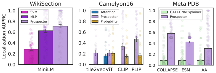
Figure 4: Prospectors vs. baselines for sequences (left), images (middle), and graphs (right). Dots represent performance on individual test-set examples, while bars represent means with standard deviations. Numerical results are found in Section B.7.

The choice of encoder is important for optimal prospector performance.

While prospectors improve localization performance over baselines regardless of the chosen encoder, the performance gain is maximized by choosing specialized encoders for each dataset. For both pathology and protein datasets, the combination of prospectors with FM encoders (CLIP, PLIP, COLLAPSE, and ESM2) outperforms non-FM encoders (tile2vec, ViT, and AA), as shown in Figure 4. Among FMs, the best-performing encoders are those with the most task-specificity — PLIP has a domain advantage by virtue of being a CLIP-style model with a vision encoder trained on pathology images, while COLLAPSE accounts for complex 3D atomic geometry rather than simply amino acid sequence (as in ESM2) or one-hot encoding (AA).

Coarse supervision and region characteristics affect localization performance.

Next, we explore the relationship between the properties of the class-specific regions and the localization performance of prospectors. To characterize class-specific regions, we compute two metrics: region prevalence (# class₁ tokens / # tokens), a proxy for coarse supervision [52] as described in Section 3.1, and mean region dispersion (# connected components / mean component size). We plot the relationship between AUPRC and both metrics in Figure 5, where each scatterplot point is a test-set example. In terms of region prevalence, we observe that for some encoders AUPRC seems to exhibit a positive correlation with prevalence across all modalities. However, some encoders achieve high AURPC even with low region prevalence (MiniLM, PLIP, COLLAPSE), while others display strong correlation (tile2vec, ViT, CLIP, AA). The metal-binding protein task is particularly challenging as the majority of its class-specific regions are below 0.1 prevalence, but prospectors were nonetheless able to achieve high performance on most test set examples. Interestingly, ESM2 showed bimodal performance, with high AUPRC on one subset and a correlated, low performance on another. This suggests that a subset of data does not contain clear sequence patterns that are correlated with zinc binding, while structure-based encoders can capture local interactions between residues far apart in sequence. In addition to the prevalence of class-specific regions, mean region dispersion provides a view into their spatial organization. In general, we see a negative correlation between the localization performance and region dispersion. These results also reflect the different characteristics of each task: the pathology test set contains a wide range of dispersion values, while the protein task contains the highest absolute levels of dispersion. Despite these task differences, prospector-equipped FM encoders demonstrate the most robustness to dispersion across modalities.

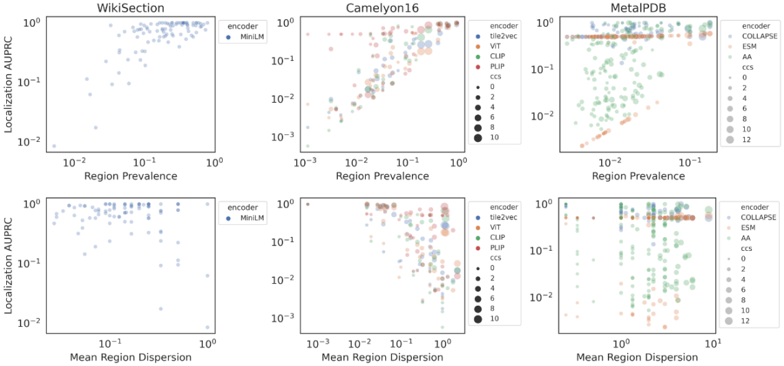
Figure 5: Prospector performance with respect to coarse supervision and region characteristics. Each point is a test-set example, colored by attached encoder and size scaled by # connected components (in Camelyon16 and MetalPDB). The more that points gravitate to the top of each plot, the more robust an encoder-prospector pair is to target region characteristics.

Prospectors’ parameters and data structures are interpretable and enable data visualization.

In addition to improved localization performance, prospectors are inherently interpretable because their parameters provide insights into class-specific patterns. Prospect maps visualize the feature attribution outputs in the input token space — but importantly, these maps can be further contextualized by visualizing the internals of the prospector head itself. Due to the use of learned semantic concepts, the global convolutional kernel can be represented graphically, along with each input example as it passes through each layer of the prospector head (Section A.2).

We illustrate this for pathology images (Figure 6) and protein structure (Figure 7) using two test set examples. For each, we first visualize the data sprites, which reflect the learned concepts mapped onto the data inputs — the outputs of quantization in layer I. By analyzing the spatial patterns of different semantic concepts on the data sprite, it is possible to assign biological or mechanistic meaning to each concept. Additionally, by visualizing the counts of the concepts and their co-occurrences in the sprite embedding, we can identify patterns are over- or under-represented within each input. By visualizing the global kernel, which captures dataset-wide concept associations and their correlations with class labels, it is possible to cross-reference between the data sprite and the class-specific regions of the resulting prospect map. The ability to visualize the internals of a prospector head in terms of concepts facilitates human-in-the-loop model development and the incorporation of domain knowledge, a major advantage relative to black box models.

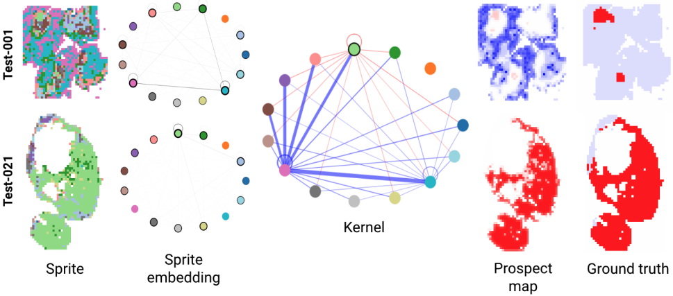
Figure 6: Prospector visualization for histopathology. The following visualizations are shown for two test set examples, from left to right: data sprites; sprite embeddings represented as self-complete graphs (Section A.2), where line thicknesses represent the monogram or skip-bigram count; the prospector head’s kernel as a self-complete graph, where line thickness is the weight learned by the kernel; prospect map, with vertex attribution scores mapped back onto tokens in the original datum; and ground-truth class-specific regions in the image (in red). Sprites and sprite embeddings are colored by the $k$ learned concepts (here, $k=15$). Kernel weights and prospect maps are colored red and blue to reflect class₁-specific and class₀-specific associations, respectively.

Further analysis of the parameters of the learned model can also help to better understand the nature of the discovered patterns. For example, there may be more than one pattern which results in a particular class label, and differentiating examples that exhibit each pattern can uncover mechanistic subgroups of the data. To demonstrate this, we hierarchically cluster the sample-level sprite embeddings in the MetalPDB test set. This identified two major subgroups of zinc binding sites (see Figure 12) defined by the number of cysteine residues coordinating the bound ion. In one subgroup, most proteins contain four coordinating cysteines, while in the other there are one or more histidine residues involved in the binding interaction. Figure 7 shows an example from each cluster, including a visualization of the zinc-binding site on the far right. This finding recapitulates known subtypes of zinc binding motifs [67], and more broadly demonstrates the potential for prospectors to discover new biological mechanisms when applied to less well-studied phenomena.

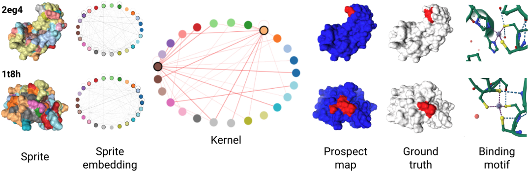
Figure 7: Prospector visualization for protein data. We show the same five visualizations as before, as well as a visualization of the atomic configuration of the zinc binding site to illustrate the binding motifs discovered by sprite embedding clustering (Figure 12). Whole proteins are shown as surface representations instead of graphs for visualization clarity.

5 Discussion & Conclusion

In summary, we present prospector heads, a (a) data-efficient, (b) computationally efficient, and (c) more accurate feature attribution technique. We show that prospectors generalize well across disparate data modalities. In addition, despite a preference for task-specific FM encoders, prospectors are encoder-agnostic (across learning regime, architecture, embedding dimension, and context sizes), provide improved attribution regardless of model choice. We note that no single baseline method could be applied universally across all datasets, requiring the use of different baselines for each experiment. Nonetheless, practically off-the-shelf, prospectors were able to outperform modality-specific methods in all experiments. This improvement is despite being much more parameter- and data-efficient — with linear time complexity with respect to data dimensionality (Section A.5) — and more interpretable through the use of a concept-based kernel.

The improved localization performance of prospectors over explanation-based methods calls into question the assumption that underlies the use of explanations for feature attribution: that end-to-end classifiers implicitly segment data in the input feature space en route to making class predictions. Our results suggest that using machine-derived concepts and modeling class-specific associations directly in the input token space helps to avoid such modeling assumptions.

A key driver of the performance of prospectors is the combination of token-level representations with the local inductive bias provided by a unified graph representation and the K2conv convolutional kernel. Our results suggest that FMs in particular have a strong sense of distributional semantics which is sufficient for high-precision feature attribution even with partial-context encoders and only weak supervision. The robustness to varying prevalence or dispersion of the target regions also suggests that prospectors do capture long-range dependencies despite operating over tokens. Additionally, because domain-specific FMs do improve performance when they are available (e.g., PLIP vs. CLIP), we hypothesize that as FMs continue to improve and be adapted to new applications and data modalities, so will the utility of prospectors across diverse domains.

Prospectors are flexible and modular by design, enabling simple changes to not only the encoder but also the training method. Of the two variants we trained, we found that the parameter-free variant was superior for all evaluated tasks (Section B.2). This may be because the hypothesis test framework requires learning dataset-wide concept associations (whereas linear models are more biased towards datum-level patterns) or because it relies on detecting deviations from a class₀ background, which is more closely modeled after the MIA (Section 3.1). It’s possible that different training methods may be better suited to detecting different types of class-specific patterns, but further investigation is needed to explore this.

One of the limitations of this work is that we were not able to test the impact of every design choice in our prospector experiments. For example, we relied on domain knowledge to select token resolution and connectivity for each task, but a more detailed study could yield greater insight into the impact of these choices. Furthermore, this study did not study the effect of different clustering methods in the quantization step, and we limited our experimentation to open-source models only. Future work involves implementing prospectors as Pytorch modules for GPU interoperability and exploring their utility with API-locked embedding models [12].

We anticipate many potential use cases for prospectors, particularly in tandem with other AI methods. One particular use case is to screen or classify data with FMs equipped with strong classifier heads, and then swap in prospector heads when feature attribution is required. Another use case is to use prospector-generated attributions to train downstream rationale models [36, 17, 68, 15]. In general, we believe that prospectors can provide an important part of the toolkit for improving the transparency and utility of large FMs, high-dimensional data, and large-scale datasets for biomedical and scientific applications.

6 Impact Statement

Trust and safety considerations are becoming increasingly important as machine learning becomes an increasingly prominent part of many high-impact disciplines such as science and biomedicine. This concern is particularly relevant for large black-box models such as foundation models. The goal of this work is to provide a new approach to feature attribution for large models and complex datasets to improve transparency of AI systems. It is important to note that that our method is specifically not designed to be an explanation of a model’s reasoning, and any feature attributions made by prospector heads should be carefully interpreted by the user in the context of the data domain.

7 Code Availability

Our code is made available at: https://github.com/gmachiraju/K2.

8 Acknowledgements

We thank Mayee Chen, Simran Arora, Eric Nguyen, Silas Alberti, Ben Viggiano, and B. Anana for their helpful feedback. Gautam Machiraju is supported by the Stanford Data Science scholarship program. Neel Guha is supported by the Stanford Interdisciplinary Graduate Fellowship and the HAI Graduate Fellowship.

We gratefully acknowledge the support of NIH under No. U54EB020405 (Mobilize), GM102365, LM012409, 1R01CA249899, and 1R01AG078755; NSF under Nos. CCF2247015 (Hardware-Aware), CCF1763315 (Beyond Sparsity), CCF1563078 (Volume to Velocity), and 1937301 (RTML); US DEVCOM ARL under Nos. W911NF-23-2-0184 (Long-context) and W911NF-21-2-0251 (Interactive Human-AI Teaming); ONR under Nos. N000142312633 (Deep Signal Processing); Chan-Zuckerberg Biohub; Stanford HAI under No. 247183; NXP, Xilinx, LETI-CEA, Intel, IBM, Microsoft, NEC, Toshiba, TSMC, ARM, Hitachi, BASF, Accenture, Ericsson, Qualcomm, Analog Devices, Google Cloud, Salesforce, Total, the HAI-GCP Cloud Credits for Research program, the Stanford Data Science Initiative (SDSI), and members of the Stanford DAWN project: Facebook, Google, and VMWare. The U.S. Government is authorized to reproduce and distribute reprints for Governmental purposes notwithstanding any copyright notation thereon. Any opinions, findings, and conclusions or recommendations expressed in this material are those of the authors and do not necessarily reflect the views, policies, or endorsements, either expressed or implied, of NIH, ONR, or the U.S. Government.

Finally, figures 1, 2, 3, 8, 9, and 10 were created with BioRender.com.

Appendix A Prospector Heads

A.1 Core Definitions

Definition A.1 (Map Graph).

A map graph $G(\mathcal{V},\mathcal{E})$ is a collection of vertices $\mathcal{V}$ and edges $\mathcal{E}$ connecting neighboring vertices in Euclidean space. Each vertex $v^{(i)}\in\mathcal{V}$ has features $\mathbf{x}^{(i)}$ and each edge $e^{(i\leftrightarrow j)}\in\mathcal{E}$ connects vertices $v^{(i)}$ to $v^{(j)}$.

Definition A.2 (Partial-context Encoder).

Given a map graph $G$, an encoder $f$ is considered partial-context if it produces an embedding $\mathbf{x}=f(v)\in\mathbb{R}^{d}$.

Definition A.3 (Full-context Encoder).

Given a map graph $G$, an encoder $f$ is considered full-context if it produces embeddings $[\mathbf{x}_{1}\ldots\mathbf{x}_{T}]=f(G)$, where $\mathbf{x}_{i}\in\mathbb{R}^{d}\quad\forall i=1\ldots T$.

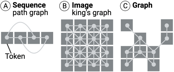
Figure 8: All unstructured data can be represented as map graphs of tokens interacting in physical space. Sequences (A) and images (B) require a specified resolution (e.g., words or sentences for text, pixels or patches for images) and connectivity (e.g., 2-hop, 8-way) for discretization.

A.2 Visualizing Prospectors

We choose to visualize any dictionaries created by prospectors (e.g., kernel $\omega$ and during rollup Section A.3.2) using self-complete graphs, which easily allow us to visualize either frequencies or importance weights for monograms and skip-bigrams. This data structure is defined below:

Definition A.4 (Self-complete graph).

A self-complete graph $K_{k}(\mathcal{V},\mathcal{E})$ is a fully connected graph with $k$ vertices, where every pair of distinct vertices $v^{(i)},v^{(j)}$ is connected by a unique edge $e^{(i\leftrightarrow j)}$. It also contains all self-edges that connect any vertex $v^{(i)}$ to itself with edge $e^{(i\leftrightarrow i)}$. Thus, self-complete graphs contain $k$ vertices and $k+{k\choose 2}$ edges.

This data structure is referenced in Figure 9, Figure 10, Figure 6, and Figure 7.

A.3 Prospector Internals & Fitting

A.3.1 Layer (I)

For all tasks, we construct our quantize layer with $k$-means clustering. Below is a schematic representation of quantization.

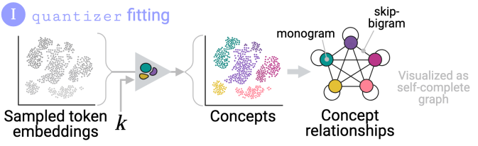
Figure 9: Prospector internals & fitting for layer (I).

A.3.2 Layer (II)

The rollup operator, named after the function of the same name in relational databases, draws similarity to a sliding bag of words featurization scheme. Internally, a dictionary $\zeta$ is constructed to capture all monograms and skip-bigrams in each neighborhood of $S$. This operator is is described by the following algorithm:

Algorithm 1 rollup

0:  Sprite $S$, receptive field $r$

1:  initialize dictionary $\zeta$

2:  for vertex $v_{i}$ in $S$ do

3:     for vertex $v_{j}$ neighborhood $\mathcal{N}_{r}$ do

4:        $\zeta\langle S[v_{i}]\rangle\leftarrow$ occurrences of concept monogram $S[v_{i}]$

5:        $\zeta\langle(S[v_{i}],S[v_{j}])\rangle\leftarrow$ occurrences of concept skip-bigram $(S[v_{i}],S[v_{j}])$

6:     end for

7:  end for

8:  return $\mathbf{z}=\operatorname{linearize}(\zeta)$ {where $\operatorname{linearize}$ returns values in sorted order}

Fitting of layer (II), along with steps 1 (rollup) and 2, is depicted in Figure 10.

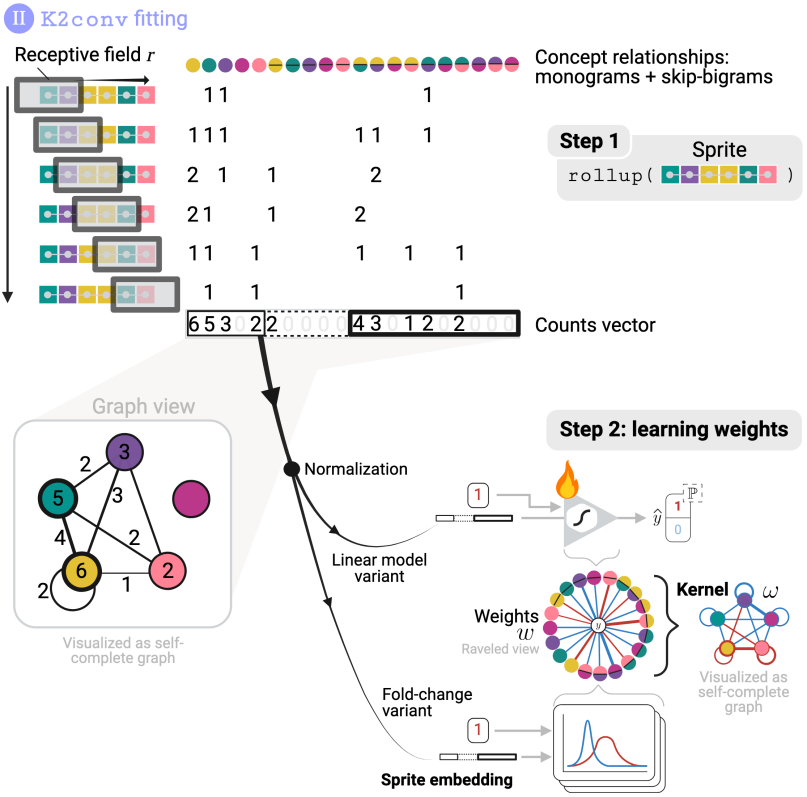
Figure 10: Prospector internals & fitting for layer (II). A flame icon indicates trainable parameters.

We note that all sprite embeddings created in rollup were normalized using TF-IDF weighting prior to kernel fitting.

A.3.3 Parameterization

Prospectors can have the following maximum number of importance weights, depending on $r$ and $k$:

$$|\mathcal{Z}|=\begin{cases}k&r=0\quad\text{(monograms only)}\\ 2k+{k\choose 2}&r>0\quad\text{(monograms \& bigrams)}\end{cases}$$

A.4 Prospector Variants

As depicted in Figure 10, and discussed in the main body of this work, we implement two variants of prospector heads: a linear classifier variant and a fold-change variant. We provide additional details here for both variants.

Linear classifier variant: This variant was implemented with the sklearn python package. The elastic net classifiers ($\lambda=0.5$) trained for a maximum of 3000 iterations using the saga solver.

Fold-change variant: In order to supply an alternative to regularization for fold-change variants, we use two-way thresholding as inspired by differential expression analysis [5]. These thresholds offer a form of masking importance weights $w_{i}\in\mathbf{w}$. As described in the main body of this work, the first threshold is $\tau$, or the minimum fold-change required. The other threshold is $\alpha$, which is a threshold used for a statistical hypothesis test, which is tests for independent class means. This test is conducted for each weight entry $w_{i}$ in $\mathbf{w}$ and significance is assessed via a Mann-Whitney U hypothesis test. Prior to weight masking, given the number of independent tests being conducted, we adjust our chosen significance threshold using the commonly used Bonferroni correction: our original $\alpha$ threshold is divided by the number of entries in $\mathbf{w}$ ($|\mathcal{Z}|$), i.e., $\alpha^{*}:=\alpha/|\mathcal{Z}|$. Finally, to perform masking: we use $\pm\tau$ to mask out sufficiently small absolute fold changes (e.g., $\pm$1, which indicates a requirement for doubling in $\log_{2}$-scale), and use $\alpha^{*}$ to mask out non-significant differences assessed by our hypothesis test.

Details on hyperparameter selection $\lambda,\tau,\alpha$ are discussed in Section B.1.

A.5 Inferential Time Complexity

We perform runtime analysis over two main variables in computation: the (tunable) number of tokens $T=|\mathcal{V}|$ and the number of forward passes $F$ of the underlying encoder. Given these variables, prospectors require only $\mathcal{O}(T)$ computations per layer: $\mathcal{O}(T)$ to quantize each token and $\mathcal{O}(T)$ to traverse over all tokens during convolution. Because prospectors are equipped to backbone encoders, full-inference must account for the encoder’s computational costs as well. Namely, an encoder requires $\mathcal{O}(F)$ for inference with full context and $\mathcal{O}(TF)$ for partial context (since each prespecified token requires a forward pass). Thus, total computational complexity of an encoder-prospector model operating on a single input datum is $\mathcal{O}(TF)$ for partial-context encoders and $\mathcal{O}(T+F)$ for full-context encoders.

For a few comparisons in full-context settings, SHAP [48] requires $\mathcal{O}(F2^{T})$ computations and DASP [4] requires $\mathcal{O}(FT^{2})$ computations per datum. We also note that $T$ is not tunable for either of these methods.

A.6 Other Properties

Prospectors can be considered a “glocal” form of attribution since they learn global, dataset-wide patterns (via their kernels) in order to construct local, input-specific attributions. Furthermore, prospectors build nonlinear maps that are shift- and rotation-equivariant, and are thus order-free and deterministic [13].

A.7 Connections to Works Beyond Feature Attribution

Our preprocessing step with concept-based token quantization has connections to previous work. Historically, constellation models [65] used vector quantization on a datum’s features before learning their spatial associations. More recently, embedding adaptation has seen success for object recognition [46] and feature attribution [24].

Our graph convolutional layer also has connections to other work. Prospectors learn spatially resolved feature associations, not unlike the associative memory of Hopfield Networks [33, 34, 46] and the learned skip-trigrams and look-up functionality of Transformers. Prospectors specifically build a kernel similar to the notion of associative memory, but with concept skip-bigrams alone to foster parameter efficiency. Finally, prospectors leverage efficient data structures and modeling primitives like linear-time convolution and learnable dictionaries [50] to efficiently scale feature attribution to high-dimensional data.

Appendix B Experimental details

B.1 Prospectors: Hyperparameter Tuning via Grid Search

For each task, we conduct a grid-search of hyperparameter configurations to select an optimal prospector model. The prospector kernel has two main hyperparameters—the number of concepts $k$ and the skip-gram neighborhood radius $r$. We also evaluate two prospector variants based on how the kernel is trained: hypothesis testing (with additional hyperparameters for the p-value $\alpha$ and fold change $\tau$ cutoffs) and linear modeling (with elastic net mixing hyperparameter $\lambda)$. We describe all tested hyperparameters in our training grid search in Table 2.

Table 2: Hyperparameters tuned during training grid search. Note: edge cutoff, the distance cutoff to control graph density, only applies to MetalPDB. We use $\infty$ to represent any large number that acts as a non-threshold.

Name	WikiSection	Camleyon16	MetalPDB
Token resolution	sentence	$224\times 224$ patch	atom
Token connectivity	2-hop	8-way	-
Concept count ($k$)	{10,15,20,25,30}	{10,15,20,25,30}	{15, 20, 25, 30}
Receptive field ($r$)	{0,1,2,4,8}	{0,1,2,4,8}	{0,1,2,4}
Significance threshold ($\alpha$)	{0.01,0.025,0.05,$\infty$}	{0.01,0.025,0.05,$\infty$}	{0.001,0.01,0.05,0.5,$\infty$}
Fold-change threshold ($\tau$)	{0,1,2}	{0,1,2}	{0,1,2,4}
Regularization factor ($\lambda$)	0.5	0.5	{0.0,0.5,1.0}
Edge cutoff ($c$)	-	-	{4.0, 6.0, 8.0}

B.2 Prospectors: Model Selection

To select a top prospector configuration after the training grid-search, we first compute four token-level evaluation metrics for training set localization and apply sequential ranking over those chosen metrics. Applied in order, our chosen metrics were: precision, Matthews correlation coefficient (MCC), Dice coefficient, and AUPRC. These metrics were chosen because they enable segmentation-style evaluation, and we preferentially select on precision because it is especially important for detecting the small-scale class-specific regions in our data. For metrics that require a threshold (precision, MCC, and Dice coefficient), we select models based on the highest value attained over 11 thresholds: $0.0,0.1,\dots,1.0$. Top prospectors per encoder, selected from the grid search and sequential ranking, are listed in Table 3.

Table 3: Top prospectors per encoder, after model selection and sequential ranking. All selected prospectors except AA are parameter-free fold-change variants. ^∗The AA encoder does not use clustering for quantization, since amino acids are already a discrete set of 21 tokens (20 standard amino acids + 1 entry for any non-standard amino acid).

Encoder Alias	$k$	$r$	$\tau$	$\alpha$	$\lambda$	$c$
MiniLM	25	1	1	0.05	-	-
tile2vec	20	8	0	$\infty$	-	-
ViT	20	2	0	0.05	-	-
CLIP	30	2	2	$\infty$	-	-
PLIP	15	1	2	0.01	-	-
COLLAPSE	15	1	4	0.5	-	8.0
ESM2	30	1	1	0.5	-	4.0
AA	21∗	2	-	-	1.0	6.0

B.3 Test Set Evaluation

After prospect graphs are created by prospector heads, we map back the values of each token to its original coordinates (referred to in the main body as prospect maps). Prior to evaluation, we feature scale values to $[0,1]$. For reporting results on the held-out test set we focus on AUPRC to provide a threshold-agnostic evaluation of each method.

B.4 Construction of Task Datasets

B.4.1 Sequences (WikiSection)

Wikisection’s disease annotated subset contains $n=3231$ documents total with 2513 training examples and 718 test examples. We preprocess the data into classes by searching each document for the presence of disease.genetics section labels. If this section label is found, we assign a document-level label of class₁ and class₀ otherwise. Because our task is at the sentence-level, we then create tokens by breaking sections into sentences by the full-stop delimiter (.). We then label sentences by their source section labels. Raw-text sentences are then fed into our chose encoder, which handles natural language tokenization.

B.4.2 Images (Camelyon16)

This benchmark contains 400 gigapixel whole slide images (270 train, 130 test) of breast cancer metastases in sentinel lymph nodes. All images were partitioned into prespecified patch tokens (size $224\times 224$) and filtered for foreground tissue regions (as opposed to the glass background of the slide). This process resulted in more than 200K unique patches without augmentation. For ground truth annotations, binary masks were resized with inter-area interpolation and re-binarized (value of 1 is assigned if interpolated value $>0$) to match the dimensionality of data sprites.

We also visualize the token embedding spaces of our encoders for the image task in Figure 11. The lack of natural clustering of class₁-specific tokens (thick $\boldsymbol{\times}$ markers) from class₀ tokens ($\circ$ markers) intuitively depicts the difficulty of our task. In other words, class-specific regions are made up of tokens that are conceptually similar to non-region tokens.

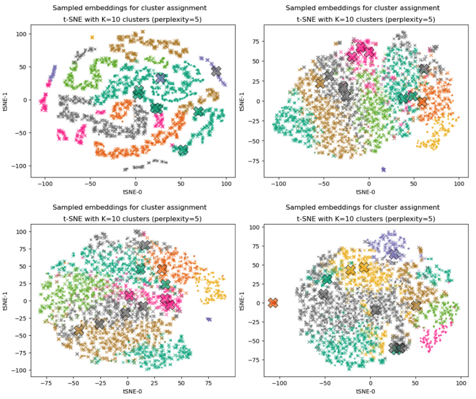
Figure 11: t-SNE plots, left-to-right then top-to-bottom: tile2vec, ViT, CLIP, PLIP. Marker color denotes concept, marker type denotes ground truth annotation for a patch: $\circ$ for class₀, $\times$ for patches from class₁ images that do originate from target regions, and the much thicker $\boldsymbol{\times}$ for class₁-specific target regions.

B.4.3 Graphs (MetalPDB)

We constructed a binary classification dataset of zinc-binding and non-binding proteins from the MetalPDB dataset [53]. We specifically focus on proteins annotated as enzymes, since metal ions are often critical for enzymatic activity. Such enzymes are known as metallo-enzymes, and our global classification labels reflect whether a metallo-enzyme relies on zinc or a different metal ion. For the positive set, we consider only biologically-relevant zinc ions which occur within a chain (i.e., are bound to residues in the main chain of the protein, rather than ligand-binding or crystallization artifacts). We sample only one protein chain from each enzymatic class, as determined by Enzyme Commission numbers [8], selecting the structure with the best crystallographic resolution. This process resulted in 756 zinc-binding sites from 610 proteins, with 653 corresponding non-zinc-binding proteins sampled from unique enzymatic classes using the same procedure. For each zinc ion in the positive set, we extract all interacting residues annotated in MetalPDB to serve as our ground truth nodes for feature attribution. This dataset was split by enzyme class to ensure that no enzyme exists in both train and test sets, reserving 20% of chains for held-out evaluation. After removing four structures which produced embedding errors, this produced a training set of 1007 unique protein chains for the train set and 252 for the test set. Each protein is featurized as a graph where each node represents a residue and edges are defined between residues which share any atom within a distance of $c$ angstroms, where $c$ varies the density of the graph.

B.5 Encoder Training

We train two backbone encoders to equip with prospectors for the image task (Camelyon16):

tile2vec: This encoder uses a ResNet-18 architecture [32] trained for 20 epochs on a single NVIDIA T4 GPU. For training, the training set of 200K patches were formed into nearly 100K triplets with a sampling scheme that chose adjacent patches as neighboring examples and patches from other images as distant examples [37]. These triplets were then used to train tile2vec with the triplet loss function [37].

ViT: We trained a custom ViT for trained for 30 epochs on a single NVIDIA T4 GPU. It was trained to perform IID patch predictions under coarse supervision, which involved image-level label inheritance [49] — the process of propagating image-level class labels to all constituent patches.

B.6 Baseline Feature Attribution Methods

B.6.1 Sequences (WikiSection)

Support vector machine (SVM): Using our sampled training embeddings from clustering, we train a one-class SVM on class₀ token embeddings ($n=4809$) to perform novelty detection on the held-out test set. The SVM was implemented with the sklearn package and trained with an RBF kernel and hyperparameter $\gamma=1/d$ (where $d$ is embedding dimension). Training ran until a stopping criterion was satisfied with 1e-3 tolerance.

Multi-layer perceptron (MLP): Using our sampled training embeddings from clustering, we train an MLP on all ($n=5000$) token embeddings (labeled as class₀ or class₁) to perform fully supervised token classification held-out test set — acting as a stand-in for a segmentation-like baseline. The MLP was implemented with the sklearn package and trained with one hidden layer (dimension 100), ReLU activations, adam optimizer, L2-regularization term of 1e-4, initial learning rate 1e-3, and minibatch size of 200. Training ran for a maximum of 1000 iterations, where inputs are shuffled.

B.6.2 Images (Camelyon16)

For this task, baselines were chosen due to their popularity and efficiency.

Concatenated mean attention (ViT only): attention maps are created per input token and their values are averaged. This creates a single attention score per token, after which tokens are concatenated by their spatial coordinates. These values are scaled to values in $[0,1]$.

Concatenated prediction probability: For ViT, each token’s prediction probability for class₁ is used to score each token, after which tokens are concatenated by their spatial coordinates. For both vision-language models, CLIP and PLIP, we prompt both FMs’ text encoders with zero-shot classification labels for class₀ and class₁, respectively: [normal lymph node, lymph node metastasis]. These labels match the benchmark dataset’s descriptions of class labels. Similarly to ViT, each token’s class₁ prediction probability is used to score each token, after which tokens are concatenated by their spatial coordinates

B.6.3 Graphs (MetalPDB)

GAT head + GNNExplainer: Our baseline for zinc binding residue identification is a graph attention network (GAT) [62] containing two GAT layers with 100 hidden features, each followed by batch normalization, followed by a global mean pooling and a fully-connected output layer. The input node features for each residue were given by the choice of encoder (COLLAPSE, ESM2, or AA). The GAT model was trained using weak supervision (i.e., on graph-level labels $y$) using a binary cross-entropy loss and Adam optimizer with default parameters and weight decay of $1\times 10^{-4}$. To select the best baseline model, we use a gridsearch over the edge cutoff for the underlying protein graph (6.0 or 8.0 Å) and the learning rate ($1\times 10^{-5}$, $1\times 10^{-4}$, $5\times 10^{-4}$, $1\times 10^{-3}$). Feature attribution was performed using a GNNExplainer [69] module applied to trained models using the implementation provided by Pytorch Geometric [27]. We produce explanations for nodes (i.e., residues) only, and perform feature attribution using hard score thresholds from $0.0,0.05,\dots,0.95,1.0$. The best model was selected using the selection criteria in Section B.1. The final models for COLLAPSE, ESM2, and AA encoders used an edge cutoff of 8.0 Å and a learning rate of $5\times 10^{-4}$, with optimal thresholds of 0.7, 0.4, and 0.5, respectively.

B.7 Tabular Results

This section reports quantitative results corresponding to Figure 4.

Table 4: Tabular results for sequences (WikiSection). Top section contains baseline methods while bottom section contains prospector-equipped encoders. Boldface indicates best-in-encoder results.

Encoder-Attribution	Mean AUPRC	Error AUPRC
MiniLM-SVM	0.284	0.233
MiniLM-MLP	0.626	0.301
MiniLM-Prospector	0.711	0.289

Table 5: Tabular results for images (Camelyon16). Top section contains baseline methods while bottom section contains prospector-equipped encoders. Boldface indicates best-in-encoder results.

Encoder-Attribution	Mean AUPRC	Error AUPRC
ViT-Attention	0.158	0.251
ViT-Probability	0.207	0.280
CLIP-Probability	0.149	0.228
PLIP-Probability	0.163	0.244
tile2vec-Prospector	0.212	0.288
ViT-Prospector	0.210	0.307
CLIP-Prospector	0.330	0.368
PLIP-Prospector	0.470	0.326

Table 6: Tabular results for protein graphs (MetalPDB). Top section contains baseline methods while bottom section contains prospector-equipped encoders. Boldface indicates best-in-encoder results.

Encoder-Attribution	Mean AUPRC	Error AUPRC
COLLAPSE-GNNExplainer	0.089	0.154
ESM-GNNExplainer	0.086	0.149
AA-GNNExplainer	0.086	0.150
COLLAPSE-Prospector	0.581	0.158
ESM2-Prospector	0.426	0.188
AA-Prospector	0.307	0.335

B.8 Domain-Specific Analysis of Prospector Internals

Figure 12 displays the results of hierarchically clustering sprite embeddings for the zinc binding task.

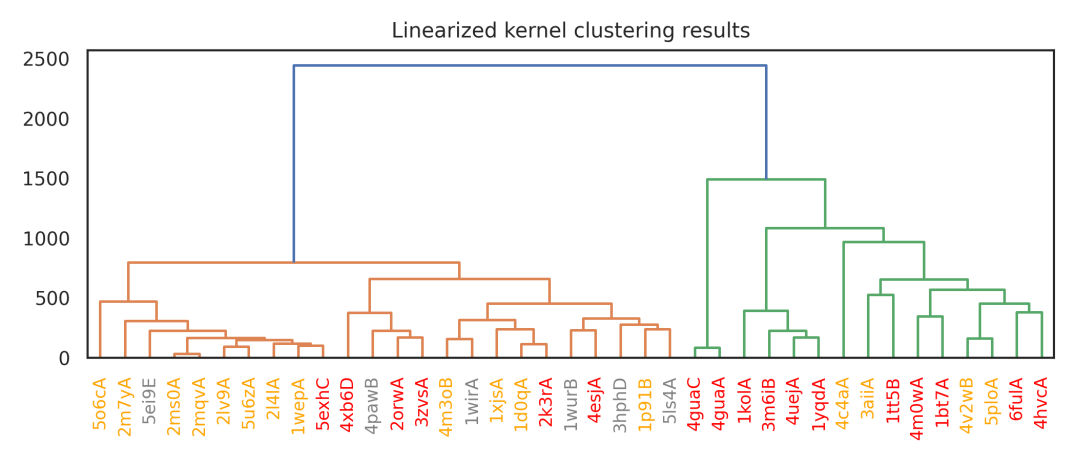
Figure 12: Hierarchical clustering results for sprite embeddings computed from high-precision test set examples. X-axis labels are colored by the number of cysteine residues coordinating the central zinc ion, which is a key feature that is correlated with the resulting clusters: gray=2, orange=3, red=4.

References

- [1] Julius Adebayo, Michael Muelly, Hal Abelson, and Been Kim. Post hoc explanations may be ineffective for detecting unknown spurious correlation. arXiv [cs.LG], December 2022.
- [2] David Alvarez-Melis and Tommi S Jaakkola. On the robustness of interpretability methods. arXiv [cs.LG], June 2018.
- [3] Jaume Amores. Multiple instance classification: Review, taxonomy and comparative study. Artif. Intell., 201:81–105, August 2013.
- [4] Marco Ancona, Cengiz Öztireli, and Markus Gross. Explaining deep neural networks with a polynomial time algorithm for shapley values approximation. arXiv [cs.LG], March 2019.
- [5] Simon Anders and Wolfgang Huber. Differential expression analysis for sequence count data. Genome Biol., 11(10):R106, October 2010.
- [6] Sebastian Arnold, Rudolf Schneider, Philippe Cudré-Mauroux, Felix A Gers, and Alexander Löser. SECTOR: A neural model for coherent topic segmentation and classification. arXiv [cs.CL], February 2019.
- [7] Nishanth Arun, Nathan Gaw, Praveer Singh, Ken Chang, Mehak Aggarwal, Bryan Chen, Katharina Hoebel, Sharut Gupta, Jay Patel, Mishka Gidwani, Julius Adebayo, Matthew D Li, and Jayashree Kalpathy-Cramer. Assessing the (un)trustworthiness of saliency maps for localizing abnormalities in medical imaging. bioRxiv, July 2020.
- [8] A Bairoch. The ENZYME database in 2000. Nucleic Acids Res., 28(1):304–305, January 2000.
- [9] Helen M Berman, Tammy Battistuz, T N Bhat, Wolfgang F Bluhm, Philip E Bourne, Kyle Burkhardt, Zukang Feng, Gary L Gilliland, Lisa Iype, Shri Jain, Phoebe Fagan, Jessica Marvin, David Padilla, Veerasamy Ravichandran, Bohdan Schneider, Narmada Thanki, Helge Weissig, John D Westbrook, and Christine Zardecki. The protein data bank. Acta Crystallogr. D Biol. Crystallogr., 58(Pt 61):899–907, June 2002.
- [10] Blair Bilodeau, Natasha Jaques, Pang Wei Koh, and Been Kim. Impossibility theorems for feature attribution. arXiv [cs.LG], December 2022.
- [11] Rishi Bommasani, Drew A Hudson, Ehsan Adeli, Russ Altman, Simran Arora, Sydney von Arx, Michael S Bernstein, Jeannette Bohg, Antoine Bosselut, Emma Brunskill, Erik Brynjolfsson, Shyamal Buch, Dallas Card, Rodrigo Castellon, Niladri Chatterji, Annie Chen, Kathleen Creel, Jared Quincy Davis, Dora Demszky, Chris Donahue, Moussa Doumbouya, Esin Durmus, Stefano Ermon, John Etchemendy, Kawin Ethayarajh, Li Fei-Fei, Chelsea Finn, Trevor Gale, Lauren Gillespie, Karan Goel, Noah Goodman, Shelby Grossman, Neel Guha, Tatsunori Hashimoto, Peter Henderson, John Hewitt, Daniel E Ho, Jenny Hong, Kyle Hsu, Jing Huang, Thomas Icard, Saahil Jain, Dan Jurafsky, Pratyusha Kalluri, Siddharth Karamcheti, Geoff Keeling, Fereshte Khani, Omar Khattab, Pang Wei Kohd, Mark Krass, Ranjay Krishna, Rohith Kuditipudi, Ananya Kumar, Faisal Ladhak, Mina Lee, Tony Lee, Jure Leskovec, Isabelle Levent, Xiang Lisa Li, Xuechen Li, Tengyu Ma, Ali Malik, Christopher D Manning, Suvir Mirchandani, Eric Mitchell, Zanele Munyikwa, Suraj Nair, Avanika Narayan, Deepak Narayanan, Ben Newman, Allen Nie, Juan Carlos Niebles, Hamed Nilforoshan, Julian Nyarko, Giray Ogut, Laurel Orr, Isabel Papadimitriou, Joon Sung Park, Chris Piech, Eva Portelance, Christopher Potts, Aditi Raghunathan, Rob Reich, Hongyu Ren, Frieda Rong, Yusuf Roohani, Camilo Ruiz, Jack Ryan, Christopher Ré, Dorsa Sadigh, Shiori Sagawa, Keshav Santhanam, Andy Shih, Krishnan Srinivasan, Alex Tamkin, Rohan Taori, Armin W Thomas, Florian Tramèr, Rose E Wang, William Wang, Bohan Wu, Jiajun Wu, Yuhuai Wu, Sang Michael Xie, Michihiro Yasunaga, Jiaxuan You, Matei Zaharia, Michael Zhang, Tianyi Zhang, Xikun Zhang, Yuhui Zhang, Lucia Zheng, Kaitlyn Zhou, and Percy Liang. On the opportunities and risks of foundation models. arXiv [cs.LG], August 2021.
- [12] Rishi Bommasani, Kevin Klyman, Shayne Longpre, Sayash Kapoor, Nestor Maslej, Betty Xiong, Daniel Zhang, and Percy Liang. The foundation model transparency index. arXiv [cs.LG], October 2023.
- [13] Michael M Bronstein, Joan Bruna, Taco Cohen, and Petar Veličković. Geometric deep learning: Grids, groups, graphs, geodesics, and gauges. arXiv [cs.LG], April 2021.
- [14] Tom B Brown, Benjamin Mann, Nick Ryder, Melanie Subbiah, Jared Kaplan, Prafulla Dhariwal, Arvind Neelakantan, Pranav Shyam, Girish Sastry, Amanda Askell, Sandhini Agarwal, Ariel Herbert-Voss, Gretchen Krueger, Tom Henighan, Rewon Child, Aditya Ramesh, Daniel M Ziegler, Jeffrey Wu, Clemens Winter, Christopher Hesse, Mark Chen, Eric Sigler, Mateusz Litwin, Scott Gray, Benjamin Chess, Jack Clark, Christopher Berner, Sam McCandlish, Alec Radford, Ilya Sutskever, and Dario Amodei. Language models are Few-Shot learners. arXiv [cs.CL], May 2020.
- [15] Kamil Bujel, Andrew Caines, Helen Yannakoudakis, and Marek Rei. Finding the needle in a haystack: Unsupervised rationale extraction from long text classifiers. arXiv [cs.CL], March 2023.
- [16] Gabriele Campanella, Matthew G Hanna, Luke Geneslaw, Allen Miraflor, Vitor Werneck Krauss Silva, Klaus J Busam, Edi Brogi, Victor E Reuter, David S Klimstra, and Thomas J Fuchs. Clinical-grade computational pathology using weakly supervised deep learning on whole slide images. Nat. Med., 25(8):1301, August 2019.
- [17] Howard Chen, Jacqueline He, Karthik Narasimhan, and Danqi Chen. Can rationalization improve robustness? arXiv [cs.CL], April 2022.
- [18] Hugh Chen, Scott M Lundberg, and Su-In Lee. Explaining a series of models by propagating shapley values. Nat. Commun., 13(1):4512, August 2022.
- [19] Peijie Chen, Qi Li, Saad Biaz, Trung Bui, and Anh Nguyen. gScoreCAM: What objects is CLIP looking at? In Computer Vision – ACCV 2022, pages 588–604. Springer Nature Switzerland, 2023.
- [20] Richard J Chen, Chengkuan Chen, Yicong Li, Tiffany Y Chen, Andrew D Trister, Rahul G Krishnan, and Faisal Mahmood. Scaling vision transformers to gigapixel images via hierarchical Self-Supervised learning. arXiv [cs.CV], June 2022.
- [21] Ian Covert, Chanwoo Kim, and Su-In Lee. Learning to estimate shapley values with vision transformers. arXiv [cs.CV], June 2022.
- [22] Jonathan Crabbé and Mihaela van der Schaar. Concept activation regions: A generalized framework for Concept-Based explanations. arXiv [cs.LG], September 2022.
- [23] Alexander Derry and Russ B Altman. COLLAPSE: A representation learning framework for identification and characterization of protein structural sites. Protein Sci., 32(2):e4541, February 2023.
- [24] Alexander Derry and Russ B Altman. Explainable protein function annotation using local structure embeddings. bioRxiv, October 2023.
- [25] Alexey Dosovitskiy, Lucas Beyer, Alexander Kolesnikov, Dirk Weissenborn, Xiaohua Zhai, Thomas Unterthiner, Mostafa Dehghani, Matthias Minderer, Georg Heigold, Sylvain Gelly, Jakob Uszkoreit, and Neil Houlsby. An image is worth 16x16 words: Transformers for image recognition at scale. arXiv [cs.CV], October 2020.
- [26] Babak Ehteshami Bejnordi, Mitko Veta, Paul Johannes van Diest, Bram van Ginneken, Nico Karssemeijer, Geert Litjens, Jeroen A W M van der Laak, the CAMELYON16 Consortium, Meyke Hermsen, Quirine F Manson, Maschenka Balkenhol, Oscar Geessink, Nikolaos Stathonikos, Marcory Crf van Dijk, Peter Bult, Francisco Beca, Andrew H Beck, Dayong Wang, Aditya Khosla, Rishab Gargeya, Humayun Irshad, Aoxiao Zhong, Qi Dou, Quanzheng Li, Hao Chen, Huang-Jing Lin, Pheng-Ann Heng, Christian Haß, Elia Bruni, Quincy Wong, Ugur Halici, Mustafa Ümit Öner, Rengul Cetin-Atalay, Matt Berseth, Vitali Khvatkov, Alexei Vylegzhanin, Oren Kraus, Muhammad Shaban, Nasir Rajpoot, Ruqayya Awan, Korsuk Sirinukunwattana, Talha Qaiser, Yee-Wah Tsang, David Tellez, Jonas Annuscheit, Peter Hufnagl, Mira Valkonen, Kimmo Kartasalo, Leena Latonen, Pekka Ruusuvuori, Kaisa Liimatainen, Shadi Albarqouni, Bharti Mungal, Ami George, Stefanie Demirci, Nassir Navab, Seiryo Watanabe, Shigeto Seno, Yoichi Takenaka, Hideo Matsuda, Hady Ahmady Phoulady, Vassili Kovalev, Alexander Kalinovsky, Vitali Liauchuk, Gloria Bueno, M Milagro Fernandez-Carrobles, Ismael Serrano, Oscar Deniz, Daniel Racoceanu, and Rui Venâncio. Diagnostic assessment of deep learning algorithms for detection of lymph node metastases in women with breast cancer. JAMA, 318(22):2199–2210, December 2017.
- [27] Matthias Fey and Jan Eric Lenssen. Fast graph representation learning with PyTorch geometric. arXiv [cs.LG], March 2019.
- [28] James Foulds and Eibe Frank. A review of Multi-Instance learning assumptions. The Knowledge Engineering Review, 0(0):1–24, 2010.
- [29] Amirata Ghorbani, James Wexler, James Zou, and Been Kim. Towards automatic concept-based explanations. arXiv [stat.ML], February 2019.
- [30] Muhammad Waleed Gondal, Jochen Gast, Inigo Alonso Ruiz, Richard Droste, Tommaso Macri, Suren Kumar, and Luitpold Staudigl. Domain aligned CLIP for few-shot classification. arXiv [cs.CV], November 2023.
- [31] Martin Halicek, Maysam Shahedi, James V Little, Amy Y Chen, Larry L Myers, Baran D Sumer, and Baowei Fei. Head and neck cancer detection in digitized Whole-Slide histology using convolutional neural networks. Sci. Rep., 9(1):14043, October 2019.
- [32] Kaiming He, Xiangyu Zhang, Shaoqing Ren, and Jian Sun. Deep residual learning for image recognition. arXiv [cs.CV], December 2015.
- [33] J J Hopfield. Neural networks and physical systems with emergent collective computational abilities. Proc. Natl. Acad. Sci. U. S. A., 79(8):2554–2558, April 1982.
- [34] J J Hopfield. Neurons with graded response have collective computational properties like those of two-state neurons. Proc. Natl. Acad. Sci. U. S. A., 81(10):3088–3092, May 1984.
- [35] Zhi Huang, Federico Bianchi, Mert Yuksekgonul, Thomas Montine, and James Zou. Leveraging medical twitter to build a visual–language foundation model for pathology AI. bioRxiv, page 2023.03.29.534834, April 2023.
- [36] Sarthak Jain and Byron C Wallace. Attention is not explanation. arXiv [cs.CL], February 2019.
- [37] Neal Jean, Sherrie Wang, Anshul Samar, George Azzari, David Lobell, and Stefano Ermon. Tile2Vec: Unsupervised representation learning for spatially distributed data. In Proceedings of the AAAI Conference on Artificial Intelligence, volume 33, pages 3967–3974, July 2019.
- [38] Neil Jethani, Mukund Sudarshan, Ian Covert, Su-In Lee, and Rajesh Ranganath. FastSHAP: Real-Time shapley value estimation. arXiv [stat.ML], July 2021.
- [39] Saumya Jetley, Nicholas A Lord, Namhoon Lee, and Philip H S Torr. Learn to pay attention. arXiv [cs.CV], April 2018.
- [40] Amir-Hossein Karimi, Krikamol Muandet, Simon Kornblith, Bernhard Schölkopf, and Been Kim. On the relationship between explanation and prediction: A causal view. arXiv [cs.LG], December 2022.
- [41] Feyza Duman Keles, Pruthuvi Mahesakya Wijewardena, and Chinmay Hegde. On the computational complexity of Self-Attention. arXiv [cs.LG], September 2022.
- [42] Been Kim, Martin Wattenberg, Justin Gilmer, Carrie Cai, James Wexler, Fernanda Viegas, and Rory Sayres. Interpretability beyond feature attribution: Quantitative testing with concept activation vectors (TCAV). arXiv [stat.ML], November 2017.
- [43] Konstantin Klemmer, Esther Rolf, Caleb Robinson, Lester Mackey, and Marc Rußwurm. SatCLIP: Global, General-Purpose location embeddings with satellite imagery. arXiv [cs.CV], November 2023.
- [44] Francois Lanusse, Liam Parker, Siavash Golkar, Miles Cranmer, Alberto Bietti, Michael Eickenberg, Geraud Krawezik, Michael McCabe, Ruben Ohana, Mariel Pettee, Bruno Regaldo-Saint Blancard, Tiberiu Tesileanu, Kyunghyun Cho, and Shirley Ho. AstroCLIP: Cross-Modal Pre-Training for astronomical foundation models. arXiv [astro-ph.IM], October 2023.
- [45] Zeming Lin, Halil Akin, Roshan Rao, Brian Hie, Zhongkai Zhu, Wenting Lu, Nikita Smetanin, Robert Verkuil, Ori Kabeli, Yaniv Shmueli, Allan Dos Santos Costa, Maryam Fazel-Zarandi, Tom Sercu, Salvatore Candido, and Alexander Rives. Evolutionary-scale prediction of atomic-level protein structure with a language model. Science, 379(6637):1123–1130, March 2023.
- [46] Qun Liu and Supratik Mukhopadhyay. Unsupervised learning using pretrained CNN and associative memory bank. In 2018 International Joint Conference on Neural Networks (IJCNN), pages 01–08. IEEE, July 2018.
- [47] Ming Y Lu, Bowen Chen, Drew F K Williamson, Richard J Chen, Ivy Liang, Tong Ding, Guillaume Jaume, Igor Odintsov, Andrew Zhang, Long Phi Le, Georg Gerber, Anil V Parwani, and Faisal Mahmood. Towards a Visual-Language foundation model for computational pathology. arXiv [cs.CV], July 2023.
- [48] Scott Lundberg and Su-In Lee. A unified approach to interpreting model predictions. arXiv [cs.AI], May 2017.
- [49] Gautam Machiraju, Sylvia Plevritis, and Parag Mallick. A dataset generation framework for evaluating megapixel image classifiers and their explanations. In Computer Vision – ECCV 2022, pages 422–442. Springer Nature Switzerland, 2022.
- [50] Julien Mairal, Jean Ponce, Guillermo Sapiro, Andrew Zisserman, and Francis Bach. Supervised dictionary learning. In D Koller, D Schuurmans, Y Bengio, and L Bottou, editors, Advances in Neural Information Processing Systems, volume 21. Curran Associates, Inc., 2008.
- [51] Muhammad Khalid Khan Niazi, Anil V Parwani, and Metin N Gurcan. Digital pathology and artificial intelligence. Lancet Oncol., 20(5):e253–e261, May 2019.
- [52] Nick Pawlowski, Suvrat Bhooshan, Nicolas Ballas, Francesco Ciompi, Ben Glocker, and Michal Drozdzal. Needles in haystacks: On classifying tiny objects in large images. arXiv [cs.CV], August 2019.
- [53] Valeria Putignano, Antonio Rosato, Lucia Banci, and Claudia Andreini. MetalPDB in 2018: a database of metal sites in biological macromolecular structures. Nucleic Acids Res., 46(D1):D459–D464, January 2018.
- [54] Alec Radford, Jong Wook Kim, Chris Hallacy, Aditya Ramesh, Gabriel Goh, Sandhini Agarwal, Girish Sastry, Amanda Askell, Pamela Mishkin, Jack Clark, Gretchen Krueger, and Ilya Sutskever. Learning transferable visual models from natural language supervision. In Marina Meila and Tong Zhang, editors, Proceedings of the 38th International Conference on Machine Learning, volume 139 of Proceedings of Machine Learning Research, pages 8748–8763. PMLR, 2021.
- [55] Marco Tulio Ribeiro, Sameer Singh, and Carlos Guestrin. “why should I trust you?”: Explaining the predictions of any classifier. arXiv [cs.LG], February 2016.
- [56] Joshua Robinson, Stefanie Jegelka, and Suvrit Sra. Strength from weakness: Fast learning using weak supervision. arXiv [cs.LG], February 2020.
- [57] Ramprasaath R Selvaraju, Michael Cogswell, Abhishek Das, Ramakrishna Vedantam, Devi Parikh, and Dhruv Batra. Grad-CAM: Visual explanations from deep networks via gradient-based localization. arXiv [cs.CV], October 2016.
- [58] Karen Simonyan and Andrew Zisserman. Very deep convolutional networks for Large-Scale image recognition. arXiv [cs.CV], September 2014.
- [59] Andrew H Song, Guillaume Jaume, Drew F K Williamson, Ming Y Lu, Anurag Vaidya, Tiffany R Miller, and Faisal Mahmood. Artificial intelligence for digital and computational pathology. Nature Reviews Bioengineering, 1(12):930–949, October 2023.
- [60] Karen Sparck Jones. A STATISTICAL INTERPRETATION OF TERM SPECIFICITY AND ITS APPLICATION IN RETRIEVAL. Journal of Documentation, 28(1):11–21, January 1972.
- [61] Ashish Vaswani, Noam Shazeer, Niki Parmar, Jakob Uszkoreit, Llion Jones, Aidan N Gomez, Lukasz Kaiser, and Illia Polosukhin. Attention is all you need. arXiv [cs.CL], June 2017.
- [62] Petar Veličković, Guillem Cucurull, Arantxa Casanova, Adriana Romero, Pietro Liò, and Yoshua Bengio. Graph attention networks, 2017.
- [63] Hanchen Wang, Tianfan Fu, Yuanqi Du, Wenhao Gao, Kexin Huang, Ziming Liu, Payal Chandak, Shengchao Liu, Peter Van Katwyk, Andreea Deac, Anima Anandkumar, Karianne Bergen, Carla P Gomes, Shirley Ho, Pushmeet Kohli, Joan Lasenby, Jure Leskovec, Tie-Yan Liu, Arjun Manrai, Debora Marks, Bharath Ramsundar, Le Song, Jimeng Sun, Jian Tang, Petar Veličković, Max Welling, Linfeng Zhang, Connor W Coley, Yoshua Bengio, and Marinka Zitnik. Scientific discovery in the age of artificial intelligence. Nature, 620(7972):47–60, August 2023.
- [64] Wenhui Wang, Furu Wei, Li Dong, Hangbo Bao, Nan Yang, and Ming Zhou. MiniLM: Deep Self-Attention distillation for Task-Agnostic compression of Pre-Trained transformers. arXiv [cs.CL], February 2020.
- [65] M Weber, M Welling, and P Perona. Unsupervised learning of models for recognition. In Computer Vision - ECCV 2000, Lecture notes in computer science, pages 18–32. Springer Berlin Heidelberg, Berlin, Heidelberg, 2000.
- [66] Sarah Wiegreffe and Yuval Pinter. Attention is not not explanation. arXiv [cs.CL], August 2019.
- [67] Shirley Wu, Tianyun Liu, and Russ B Altman. Identification of recurring protein structure microenvironments and discovery of novel functional sites around CYS residues. BMC Struct. Biol., 10:4, February 2010.
- [68] Chenghao Yang, Fan Yin, He He, Kai-Wei Chang, Xiaofei Ma, and Bing Xiang. Efficient shapley values estimation by amortization for text classification. arXiv [cs.CL], May 2023.
- [69] Rex Ying, Dylan Bourgeois, Jiaxuan You, Marinka Zitnik, and Jure Leskovec. GNNExplainer: Generating explanations for graph neural networks. Adv. Neural Inf. Process. Syst., 32:9240–9251, December 2019.
- [70] John R Zech, Marcus A Badgeley, Manway Liu, Anthony B Costa, Joseph J Titano, and Eric K Oermann. Confounding variables can degrade generalization performance of radiological deep learning models. arXiv [cs.CV], July 2018.
- [71] Bolei Zhou, Aditya Khosla, Agata Lapedriza, Aude Oliva, and Antonio Torralba. Learning deep features for discriminative localization. In 2016 IEEE Conference on Computer Vision and Pattern Recognition (CVPR). IEEE, June 2016.
- [72] Yilun Zhou, Serena Booth, Marco Tulio Ribeiro, and Julie Shah. Do feature attribution methods correctly attribute features? arXiv [cs.LG], April 2021.