Invertible Fourier Neural Operators for Tackling Both Forward and Inverse Problems

Abstract

Fourier Neural Operator (FNO) is a popular operator learning method, which has demonstrated state-of-the-art performance across many tasks. However, FNO is mainly used in forward prediction, yet a large family of applications rely on solving inverse problems. In this paper, we propose an invertible Fourier Neural Operator (iFNO) that tackles both the forward and inverse problems. We designed a series of invertible Fourier blocks in the latent channel space to share the model parameters, efficiently exchange the information, and mutually regularize the learning for the bi-directional tasks. We integrated a variational auto-encoder to capture the intrinsic structures within the input space and to enable posterior inference so as to overcome challenges of illposedness, data shortage, noises, etc. We developed a three-step process for pre-training and fine tuning for efficient training. The evaluations on five benchmark problems have demonstrated the effectiveness of our approach.

1 Introduction

Operator learning (OL) is currently at the forefront of scientific machine learning. It seeks to estimate function-to-function mappings from data and can be used as a valuable surrogate in various applications related to physical simulation. These applications span a wide range, including weather forecasting (Pathak et al., 2022), adaptive control (Bhan et al., 2023), engineering design (Liu et al., 2023), urban water clarification (Li and Shatarah, 2024), etc. Among the notable approaches in this domain is the Fourier neural operator (FNO) (Li et al., 2020c). Leveraging the convolution theorem and fast Fourier transform (FFT), FNO executes a sequence of global linear transform and nonlinear activation within the functional space to flexibly capture the function-to-function mapping. While the storage of the transformation weights in the frequency domain can be memory intensive, the FNO is computationally highly efficient, and demonstrates state-of-the-art performance across various OL tasks.

Despite the many success stories, the FNO is primarily applied for solving forward problems. Typically, it is used to predict solution functions based on the input sources, parameters of partial differential equations (PDEs), and/or initial conditions. However, practical applications often involve another crucial category of tasks, namely inverse problems (Stuart, 2010). For instance, given the solution measurements, how to deduce the unknown sources, determine the PDE parameters, or identify the initial conditions? Inverse problems tend to be more challenging due to issues such as ill-posedness, noisy measurements, and limited data quantity. Even if one attempts to directly train an FNO to map the measured solution function back to the input of interest, the aforementioned challenges persist.

To bridge this gap, we propose iFNO, a novel invertible Fourier neural operator capable of addressing both forward and inverse problems while providing posterior estimation and uncertainty quantification. Due to the sharing of the model parameters, we achieve a significant reduction in model size and memory costs. More importantly, the co-learning for the bi-directional tasks facilitates efficient information exchange and mutual regularization, enhancing performance on both fronts and mitigating challenges such as ill-posedness and data noises. Specifically, we first design a series of invertible Fourier blocks in the lifted channel space, capturing rich representation information. Each block processes a pair of inputs with an equal number of channels, generating outputs through the Fourier layer of FNO, softplus transform, and element-wise multiplication. This ensures a rigorous bijection pair between the inputs and outputs during expressive functional transforms. To enable inverse prediction in the original space, we incorporate a pair of multi-layer perceptions (MLPs) that lift the final prediction’s channel back to the latent space and project latent channels to the input space. Second, to capture intrinsic structures within input functions and further overcome challenges like ill-posedness and data shortage, we introduce a low-dimensional representation and integrate a variational auto-encoder (VAE) to reconstruct the input function. The VAE component also enables the computation of posterior samples for the prediction. Third, for efficient training, we use a three-step process: we pre-train invertible blocks excluding the VAE, pre-train the VAE component, and then fine-tune the entire model.

For evaluation, we examined our method in five benchmark problems, including scenarios based on Darcy flow, wave propagation and Naiver-Stoke (NS) equations. In addition to forward solution prediction, our method was tested for inverse inference, specifically deducing permeability, square slowness, and initial conditions from (noisy) solution measurements We compared with the recent inverse neural operator (Molinaro et al., 2023) designed explicitly for solving inverse problems, and invertible deep operator net (Kaltenbach et al., 2022). Additionally, comparisons were made with training the standard FNO separately for forward and inverse problems. Across all the tasks, iFNO consistently outperforms the competing methods by a large margin in terms of prediction accuracy. The ablation study confirms the effectiveness of both our invertible blocks and VAE component. Visualization of the predictive variance for the inverse problems reveals intriguing and reasonable uncertainty calibration results.

2 Preliminaries

Operator Learning. Consider learning a mapping between two function spaces (e.g., Banach spaces) $\psi:\mathcal{H}\rightarrow{\mathcal{U}}$. We collect a training dataset that consists of pairs of discretized input and output functions, denoted by $\mathcal{D}=\{({\bf f}_{k},{\bf u}_{k})\}_{k=1}^{N}$. Each ${\bf f}_{k}$ includes samples from an input function $f_{k}\in\mathcal{H}$, and ${\bf u}_{k}$ includes samples from the output function $u_{k}=\psi(f_{k})\in{\mathcal{U}}$. Both $f_{k}$ and $u_{k}$ are sampled from evenly-spaced locations, e.g., over a 128 $\times$ 128 grid in the 2D domain $[0,1]\times[0,1]$.

Fourier Neural Operator. The FNO first lifts the (discretized) input function ${\bf f}$ into a higher-dimensional feature space (via an MLP) to enrich the representation. Then it uses a series of Fourier layers to alternatingly conduct linear transforms and nonlinear activation in the functional space,

$$v_{t+1}({\bf x})\leftarrow\sigma\left({\mathcal{W}}v_{t}({\bf x})+\int\kappa({\bf x}-{\bf x}^{\prime})v_{t}({\bf x}^{\prime}){\rm d}{\bf x}^{\prime}\right),$$ (1)

where $v_{t}({\bf x})$ is the input function to the $t$-th layer, $v_{t+1}(x)$ the output function, $\kappa$ the integration kernel, and $\sigma$ the activation. Utilizing the convolution theorem expressed as

$$\int\kappa({\bf x}-{\bf x}^{\prime})v_{t}({\bf x}^{\prime}){\rm d}{\bf x}^{\prime}=\mathcal{F}^{-1}\left[\mathcal{F}[\kappa]\cdot\mathcal{F}[v_{t}]\right]({\bf x}),$$

where $\mathcal{F}$ and $\mathcal{F}^{-1}$ denote the Fourier and inverse Fourier transforms, respectively, the Fourier layer first executes a fast Fourier transform (FFT) over $v_{t}$, then multiplies the result with the discretized representation of $\kappa$ in the frequency domain, i.e., $\mathcal{F}[\kappa]$, and executes inverse FFT. The local linear transform $\mathcal{W}v_{t}(\mathbf{x})$ is achieved through standard convolution. Owning to FFT, the Fourier layer is computationally highly efficient. Note that, however, the storage of $\mathcal{F}[\kappa]$ (global transformation weights) can be memory intensive, even after truncating the high frequency modes. After several Fourier layers, another MLP is used to project back from the latent space to generate the final prediction. The training is typically carried out by minimizing a relative $L_{2}$ loss,

$$\Theta^{*}=\operatornamewithlimits{argmin}_{\Theta}\frac{1}{N}\sum_{n=1}^{N}\frac{\|{\bf u}_{n}-\psi_{\text{FNO}}({\bf f}_{n};\Theta)\|}{\|{\bf u}_{n}\|},$$ (2)

where $\|\cdot\|$ is often chosen as the Frobenius norm, and $\Theta$ includes all the model parameters.

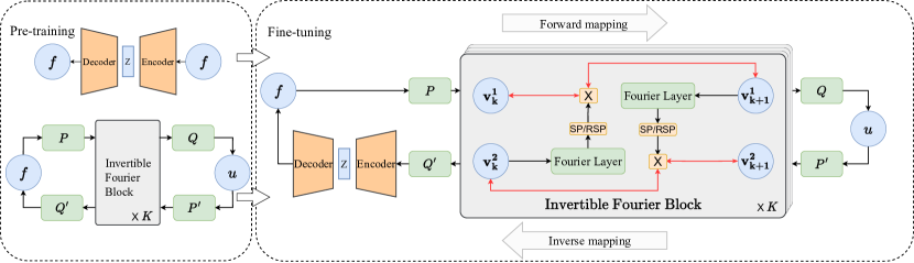
Figure 1: An overview of iFNO. Left panel: the $\beta$-VAE module and the invertible Fourier blocks. Right panel: the entire architecture. “SP” and “RSP” denote softplus and the reciprocal of the softplus, respectively. During training, we first pre-train the $\beta$-VAE module and invertible Fourier blocks as shown in the first panel. Then we fine-tune the entire model as depicted in the right panel.

3 Invertible Fourier Neural Operators

Neural operators, including FNO, are commonly employed to address forward problems, namely predicting or computing the outcomes based on given inputs to the system of interest. Taking PDE systems as an example, the input function typically comprises external sources or forces, system parameters, and/or initial conditions, with the output representing the corresponding solution function. However, practical applications frequently involve a keen interest in deducing unknown causes from observed effects, a scenario known as inverse problems. For instance, this involves inferring unknown sources, system parameters, or initial conditions from solution measurements. Inverse problems have broad significance in scientific and engineering domains, including applications in mechanics  (Tanaka and Dulikravich, 1998), geophysics  (Yilmaz, 2001), and medical imaging  (Nashed and Scherzer, 2002). However, tackling inverse problems is notably challenging due to their inherently ill-posed nature. In contrast to forward problems, inverse problems often lack a unique solution and are highly sensitive to variations in data. These challenges are further compounded in practical applications where measurement data is often limited, noisy, and/or inaccurate.

To address these challenges and to fill the gap of the current work, we propose iFNO, an invertible Fourier neural operator for tackling both the forward and inverse problems. Specifically, given the training dataset $\mathcal{D}=\{{\bf f}_{k},{\bf u}_{k}\}_{n=1}^{N}$, our goal is to jointly learn the forward and inverse mappings via a unified neural operator,

$$\psi:\mathcal{H}\rightarrow{\mathcal{U}},\;\;\;\;\psi^{-1}:{\mathcal{U}}\rightarrow\mathcal{H}.$$ (3)

By sharing the model parameters for both tasks, not only can we substantially reduce the model size and the associated memory cost, the co-learning for the bi-directional tasks enables efficient information exchange and mutual regularization, improving performance on both fronts and alleviating aforementioned challenges like ill-posedness and data noise. The details of iFNO are specified as follows.

3.1 Invertible Fourier Blocks in Latent Space

To enable invertible computing and prediction while preserving the expressiveness of the original FNO, we first design and stack a series of invertible Fourier blocks in the latent channel space. Specifically, following the standard FNO, we apply an MLP $\mathcal{P}$ over each element of the discretized input function ${\bf f}$ (and the sampling locations) so as to map ${\bf f}$ into a higher-dimensional latent space with $2d$ channels. That is, at each sampling location, we have a $2d$-dimensional feature representation. We split the channels of $\mathcal{P}({\bf f})$ into halves, each with $d$ channels, and feed them into a series of invertible Fourier blocks $\mathcal{IF}_{1},\ldots,\mathcal{IF}_{K}$. Each block $\mathcal{IF}_{k}$ receives a pair of inputs ${\bf v}^{1}_{k}$ and ${\bf v}^{2}_{k}$, and produces a pair of outputs ${\bf v}^{1}_{k+1}$ and ${\bf v}^{2}_{k+1}$, which are then fed into the next block $\mathcal{IF}_{k+1}$. All the input and outputs possess the same number of channels. We use the framework in (Dinh et al., 2016) to design each block $\mathcal{IF}_{k}$,

$${\bf v}_{k+1}^{1}\leftarrow {\bf v}_{k}^{1}\odot S(\mathcal{L}({\bf v}_{k}^{2})),$$

$${\bf v}_{k+1}^{2}\leftarrow {\bf v}_{k}^{2}\odot S(\mathcal{L}({\bf v}_{k+1}^{1})),$$ (4)

where $\odot$ is the element-wise multiplication, $\mathcal{L}$ is the Fourier layer of the original FNO that fulfills the linear functional transform and nonlinear activation as expressed in (1), and $S$ is the element-wise softplus transform,

$$S(x)=\frac{1}{\tau}\log\left(1+\exp(\tau x)\right),$$ (5)

where $\tau$ is a hyperparameter to adjust the shape. We can see that $\{{\bf v}^{1}_{k},{\bf v}^{2}_{k}\}$ and $\{{\bf v}^{1}_{k+1},{\bf v}^{2}_{k+1}\}$ therefore form a bijection pair. Given the outputs $\{{\bf v}_{k+1}^{1},{\bf v}_{k+1}^{2}\}$, the inputs can be inversely computed via

$${\bf v}_{k}^{2} \leftarrow{\bf v}_{k+1}^{2}\odot\left[S(\mathcal{L}({\bf v}_{k+1}^{1}))\right]^{-1},$$

$${\bf v}_{k}^{1} \leftarrow{\bf v}_{k+1}^{1}\odot\left[S(\mathcal{L}({\bf v}_{k}^{2}))\right]^{-1},$$ (6)

where $[\cdot]^{-1}$ denotes the element-wise reciprocal.

The outputs of the last invertible Fourier block, ${\bf v}^{1}_{K}$ and ${\bf v}^{2}_{K}$, are concatenated and fed into a second MLP ${\mathcal{Q}}$, which projects back to generate the prediction of the solution function (at sampled locations),

$$\psi_{\text{iFNO}}({\bf f})={\mathcal{Q}}({\bf v}^{1}_{K},{\bf v}^{2}_{K}).$$ (7)

Next, to fulfill the inverse prediction from the (discretized) output function ${\bf u}$ back to the input function, we introduce another pairs of MLPs, $\mathcal{P}^{\prime}$ and ${\mathcal{Q}}^{\prime}$, for which, $\mathcal{P}^{\prime}$ first maps ${\bf u}$ back to the latent space to predict the outputs of the last invertible Fourier block,

$${\bf v}^{1}_{K},{\bf v}^{2}_{K}=\mathcal{P}^{\prime}({\bf u}),$$

then inversion (6) is sequentially applied to predict the inputs to each block until the first one, and finally ${\bf Q}^{\prime}$ projects the inputs to the first invertible Fourier block back to generate the prediction of the original input function,

$$\psi^{-1}_{\text{iFNO}}({\bf u})={\bf Q}^{\prime}({\bf v}^{1}_{1},{\bf v}^{2}_{1}).$$ (8)

One might question why not position the invertible Fourier blocks directly in the original space, eliminating channel lifting and projection. However, adopting this approach will severely limit the representation power and miss the rich information in the higher-dimensional latent space. Additionally, deciding whether to split the original input function into halves or duplicate it into two copies becomes a challenge. The former can potentially disrupt the internal structures of the input function, while the latter introduces additional training issues, such as how to enforce the prediction of the two inputs to be identical. We found that, in both our model and the standard FNO, channel lifting and projection are crucial to achieve promising performance.

3.2 Embedding Intrinsic Structures

To extract the intrinsic structures within the input functions so as to better overcome the ill-posedness, data shortage and noise issues for solving inverse problems, we further integrate a $\beta$-variational auto-encoder ($\beta$-VAE) (Higgins et al., 2016) into our model. Specifically, after projecting $\{{\bf v}^{1}_{1},{\bf v}^{2}_{1}\}$ back to the input space — see (8) — we feed the results to the an encoder network to obtain a stochastic latent embedding ${\bf z}$. Then through a decoder network, we produce the prediction of the input function, namely,

$${\bf z} =\text{Encoder}\left({\mathcal{Q}}^{\prime}({\bf v}^{1}_{1},{\bf v}^{1}_{2}),{\bm{\epsilon}}\right),\;\;{\bm{\epsilon}}\sim\mathcal{N}({\bf 0},{\bf I}),$$

$${\bf f} =\psi^{-1}_{\text{iFNO}}({\bf u})=\text{Decoder}\left({\bf z}\right).$$ (9)

We leverage the auto-encoding variational Bayes framework (Kingma and Welling, 2013) to estimate the posterior distribution of ${\bf z}$. This allows us to generate the posterior samples of the inverse prediction for ${\bf f}$, enabling the evaluation of the uncertainty. Our overall model is illustrated in Fig. 1.

3.3 Three-Step Training

For effective learning, we use a three-step procedure. We first pre-train the invertible Fourier blocks without the VAE component (i.e., removing (9)). The loss is given by

$$J_{\text{IFB}}=J_{\text{FWD}}+J_{\text{INV}}+J_{\mathcal{P},{\mathcal{Q}}^{\prime}}+J_{\mathcal{P}^{\prime},{\mathcal{Q}}},$$ (10)

where

$$J_{\text{FWD}}=\frac{1}{N}\sum_{n=1}^{N}\frac{\|{\bf u}_{n}-\psi_{\text{iFNO}}({\bf f}_{n})\|}{\|{\bf u}_{n}\|},$$

$$J_{\text{INV}}=\frac{1}{N}\sum_{n=1}^{N}\frac{\|{\bf f}_{n}-\psi^{-1}_{\text{iFNO}}({\bf u}_{n})\|}{\|{\bf f}_{n}\|}$$ (11)

measure the data fitness for forward and inverse predictions, and

$$J_{\mathcal{P},{\mathcal{Q}}^{\prime}} =\frac{1}{N}\sum_{n=1}^{N}\frac{\|{\bf f}_{n}-{\mathcal{Q}}^{\prime}(\mathcal{P}({\bf f}_{n}))\|}{\|{\bf f}_{n}\|},$$

$$J_{\mathcal{P}^{\prime},{\mathcal{Q}}} =\frac{1}{N}\sum_{n=1}^{N}\frac{\|{\bf u}_{n}-{\mathcal{Q}}(\mathcal{P}^{\prime}({\bf u}_{n}))\|}{\|{\bf u}_{n}\|}$$ (12)

are two additional reconstruction loss terms that encourage the invariance of the original information after channel lifting and projection at both the input and output ends.

Next, we pre-train the $\beta$-VAE component exclusively with the samples of the input functions. This adaptation of the parameters aims to capture the hidden structures within the input function space. We minimize a variational free energy,

$$J_{\beta-\text{VAE}}=\frac{1}{N}\sum_{n=1}^{N}J_{n},$$ (13)

$$J_{n}=\beta\cdot\text{KL}(q({\bf z}_{n})\|p({\bf z}_{n}))+\mathbb{E}_{q}\left[\frac{\|{\bf f}_{n}-\text{Decoder}({\bf z}_{n})\|}{\|{\bf f}_{n}\|}\right],$$

where KL is the Kullback-Leibler divergence, $\beta$ is a hyper-parameter, ${\bf z}_{n}$ is the stochastic embedding representation of ${\bf f}_{n}$, and $q({\bf z}_{n})$ is the posterior distribution. The samples from $q({\bf z}_{n})$ is generated from the probabilistic encoder defined in (9). Note that, for pre-training, the input to the encoder network (that generates the posterior samples of $z_{n})$ is ${\bf f}_{n}$. We use the reparameterization trick for stochastic optimization.

Finally, we fine-tune the entire model by minimizing a joint loss,

$$J=J_{\text{FWD}}+J_{P,Q^{\prime}}+J_{Q,P^{\prime}}+J_{\beta-\text{VAE}},$$ (14)

where according to (9), the inverse prediction is now $\psi^{-1}_{\text{iFNO}}({\bf u}_{n})=\text{Decoder}({\bf z}_{n})$, and the input to the encoder network for each ${\bf z}_{n}$ is generated by lifting ${\bf u}_{n}$ with $\mathcal{P}^{\prime}$, going through invertible Fourier blocks, $\mathcal{IF}_{K},\ldots,\mathcal{IF}_{1}$, and then applying projection MLP ${\mathcal{Q}}^{\prime}$.

4 Related Work

Operator learning is a rapidly advancing research field, with various methods falling under the category of neural operators, primarily based on neural networks. Alongside FNO, other notable approaches have been proposed. For instance, the low-rank neural operator (LNO) (Li et al., 2020c) decomposes the operator kernel with a low-rank representation. GNO, introduced by Li et al. (2020a), leverages Nystrom approximation and graph neural networks for function convolution approximation. The multipole graph neural operator (MGNO)  (Li et al., 2020b) utilizes a multi-scale kernel decomposition to enable linear complexity in convolution computation. Gupta et al. (2021) developed a multiwavelet-based operator learning method. Another widely adopted approach is the Deep Operator Net (DeepONet) (Lu et al., 2021), which consists of a branch net and a trunk net. The branch net is applied over the discretized input function while the trunk net over the sampling locations. The prediction is generated by the dot product between the outputs of the two nets. To improve the stability and efficiency,  Lu et al. (2022) replaced the trunk net by the POD (PCA) bases. Instead of a dot product, Seidman et al. (2022) nonlinearly combined the branch net and trunc net’s outputs, such as via an MLP, to produce the prediction. The recent paper (Kovachki et al., 2023) provides a nice survey of neural operators.

Recently, Molinaro et al. (2023) proposed neural inverse operator (NIO), explicitly designed for addressing inverse problems. NIO sequentially combines DeepONet and FNO, where the DeepONet takes observations (e.g., solution measurements) and querying locations as the input, and the outputs are subsequently passed to FNO to obtain the prediction for the inverse problems. NIO does not offer uncertainty quantification. Kaltenbach et al. (2023) developed an invertible version of DeepONet. The key idea is to modify the branch net to be invertible following the framework of (Dinh et al., 2016). Given the observations, the approach starts by solving a least-squares problem to recover the output of the branch net, and then proceeds to back-predict the input function. The least-squares problem is further casted into a Bayesian inference task and a Gaussian mixture prior (constructed from training data) is assigned for the unknown output of the branch net. One potential constraint of this approach is that the input and output dimensions of the branch net must be identical for invertibility. When the dimensionality or resolution of the (discretized) input function is high, it can substantially raise computational costs and pose learning challenges (see Sec 5). The recent work (Zhao et al., 2022) aims to tackle the inverse problems with a forward graph neural network simulator (solver), called MeshGraphNet (Pfaff et al., 2020). It optimizes the input to the MeshGraphNet to align the output with the solution measurements. While effective, performing numerical optimization for every inverse prediction can be computationally expensive. Moreover, this method relies on knowledge of the underlying system (e.g., the order of derivatives in PDEs) for the inverse problem and the ability to simulate the system to generate extensive training examples for MeshGraphNet. However, in practice, such knowledge is often unavailable or inaccurate.

5 Numerical Experiments

We evaluated our method on five benchmark problems, each covering both the forward and inverse scenarios. These problems are grounded in Darcy flow, wave propagation, and Navier-Stokes (NS) equations.

5.1 Darcy Flow

We first considered a single-phase 2D Darcy Flow equation,

$$-\nabla\cdot(a({\bf x})\nabla u({\bf x})) =f({\bf x})\quad{\bf x}\in(0,1)^{2}$$

$$u({\bf x}) =0,\quad{\bf x}\in\partial(0,1)^{2},$$ (15)

where $a({\bf x})$ is the permeability field, $u({\bf x})$ is fluid pressure, and $f(x)$ is an external source. We considered a practically useful case where the permeability is piece-wise constant across separate regions $\{{\mathcal{R}}_{i}\}^{C}_{i=1}$, $a(x)=\sum_{i=1}^{C}q_{i}\mathbbm{1}_{{\mathcal{R}}_{i}}({\bf x})$. For the forward scenario, we are interested in predicting the pressure field $u({\bf x})$ based on the given permeability field $a({\bf x})$. Conversely, in the inverse scenario, the goal is to recover $a$ from the measurement of the pressure field $u$. We considered two benchmark problems, each featuring the permeability with a different type of geometric structures. For both problems, we fix $f(x)$ to $1$.

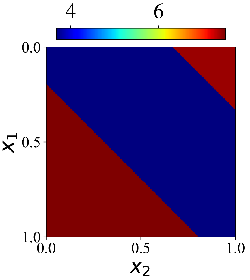
(a) Permeability

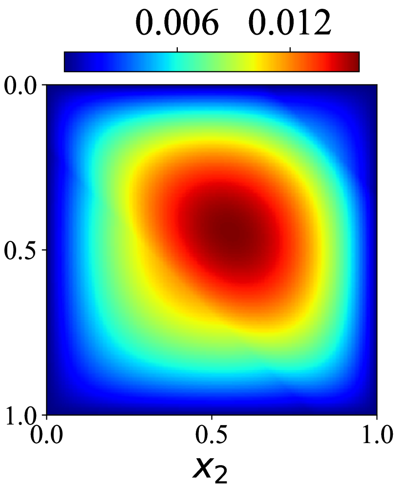
(b) Solution

Figure 5: Darcy flow with piece-wise permeability and linear interfaces.

Linear permeability interface. In the first problem, the domain was divided into three regions (namely $C=3$), and the interfaces were represented by parallel lines inclined at a 45-degree angle from the horizontal axis; see Appendix Fig. 5 for an example. The permeability in each region was sampled from a uniform distribution $U(0,10)$. To determine the position of these sections, we sampled the endpoints of interface lines, denoted by $\{(w_{1},0),(0,w_{1})\}$ for the first interface, and $\{(w_{2},0),(0,w_{2})\}$ for the second interface, respectively, where $w_{1}\sim{\mathcal{U}}(0,\frac{1}{3})$ and $w_{2}\sim{\mathcal{U}}(\frac{1}{3},\frac{2}{3})$.

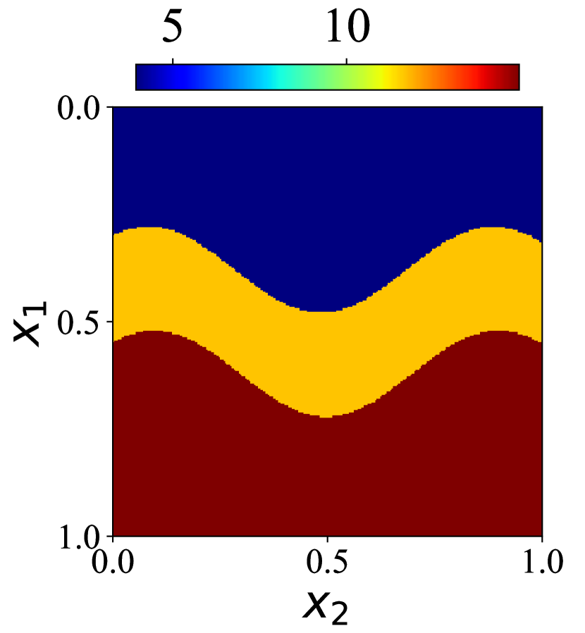
(a) Permeability

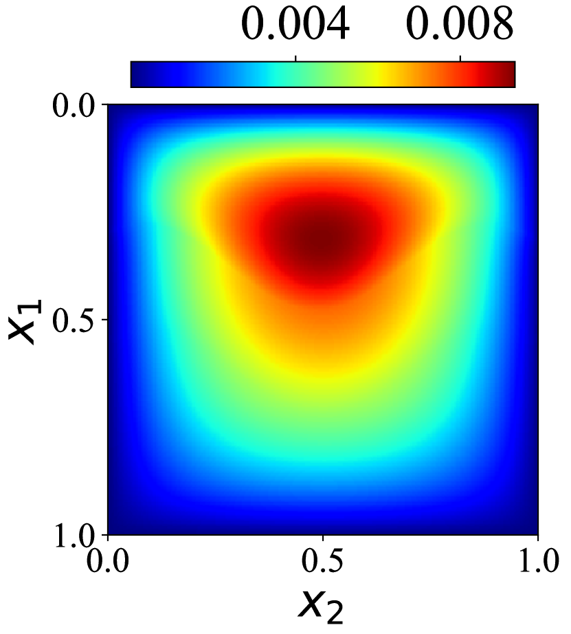
(b) Solution

Figure 6: Darcy flow with piece-wise permeability and curved interfaces.

Curved permeability interface. In the second problem, the domain was also partitioned into three regions, but the interfaces were curves; see Fig. 6 of the Appendix for an illustration. We sampled the first interface as $x_{2}=p_{1}+0.1\sin(2.5\pi(x_{1}+r_{1}))$ and the second $x_{2}=p_{2}+0.1\sin(2.5\pi(x_{1}+r_{2}))$, where $p_{1}\sim\mathcal{U}(0.15,0.4),p_{2}\sim\mathcal{U}(0.6,0.85)$, and $r_{1},r_{2}\sim\mathcal{U}(0,1)$. The permeability in each region was sampled from $U(0,15)$.

To prepare the dataset, we followed (Li et al., 2020c) to apply a second-order finite difference solver on a $253\times 253$ grid, and downsampled the permeability and pressure field to a $64\times 64$ grid. For the case of linear permeability interfaces, we used 300 training examples, while for the curved interfaces, we used 800 training examples. In both problems, we evaluated our method with 500 test examples. To assess the robustness of our method against data noise and inaccuracy, we conducted additional tests by injecting 10% and 20% white noises into the training datasets. Specifically, for each pair of ${\bf f}_{n}$ and ${\bf u}_{n}$ generated by the simulator, we corrupted them via updating ${\bf f}_{n}\leftarrow{\bf f}_{n}+\eta\bm{\sigma}_{f}\odot{{\bm{\epsilon}}_{n}}$ and ${\bf u}_{n}\leftarrow{\bf u}_{n}+\eta\bm{\sigma}_{u}\odot\bm{\xi}_{n}$, where $\eta\in\{0.1,0.2\}$ represents the noise level, $\bm{\sigma}_{f}$ and $\bm{\sigma}_{\bf u}$ are the per-element standard deviation of the sampled input and output functions, and ${\bm{\epsilon}}_{n},\bm{\xi}_{n}\sim\mathcal{N}({\bf 0},{\bf I})$ are Gaussian white noises.

5.2 Wave Propagation

We next employed an acoustic seismic wave equation to simulate seismic surveys,

$$m({\bf x})\frac{{\rm d}^{2}u({\bf x},t)}{{\rm d}t^{2}}-\nabla^{2}u({\bf x},t)+\eta\frac{{\rm d}u(x,t)}{{\rm d}t}=q(t),\;{\bf x}\in\Omega,$$

$$u({\bf x},0)=\frac{{\rm d}u(x,0)}{{\rm d}t}=0,{\bf x}\in\Omega,\;\;u({\bf x},t)=0,{\bf x}\in\partial\Omega,$$

where $m({\bf x})$ is square slowness, defined as the inverse of squared wave speed in the given physical media, $q(t)$ expresses the external wave source, and $\eta$ is the damping mask. In the simulation, the physical media was placed in the domain $\Omega=(0,1.28\,\mathrm{km})^{2}$, where $\forall{\bf x}=(x_{1},x_{2})\in\Omega$, $x_{1}$ and $x_{2}$ represent the depth and width, respectively. For each survey, an external source was positioned at particular location to initiate seismic waves. A row of receivers were placed at a particular depth to record the wave measurements across time. We conducted simulation over a duration of one second. In the forward tasks, we intended to predict the wave measurements at the receivers based on the square slowness $m({\bf x})$, while for the inverse tasks, the goal was to recover $m({\bf x})$ from the measurements at the receivers. We designed two benchmark problems, each corresponding to a different class of structures for $m({\bf x})$. In both problems, we set $q(t)=(1-2\pi^{2}f_{0}^{2}(t-\frac{1}{f_{0}})^{2})e^{-\pi^{2}f_{0}^{2}(t-\frac{1}{f_{0}})}$, where $f_{0}=0.01$. This implies that the peak frequency of the source wave is 10 Hz.

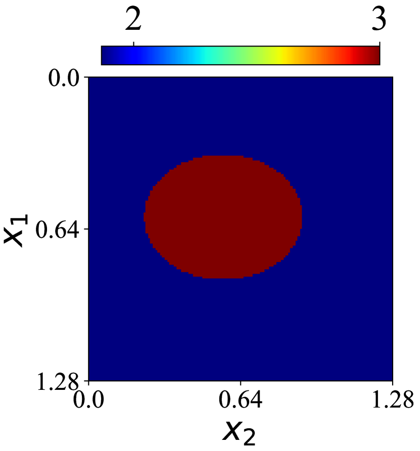
(a) Square slowness

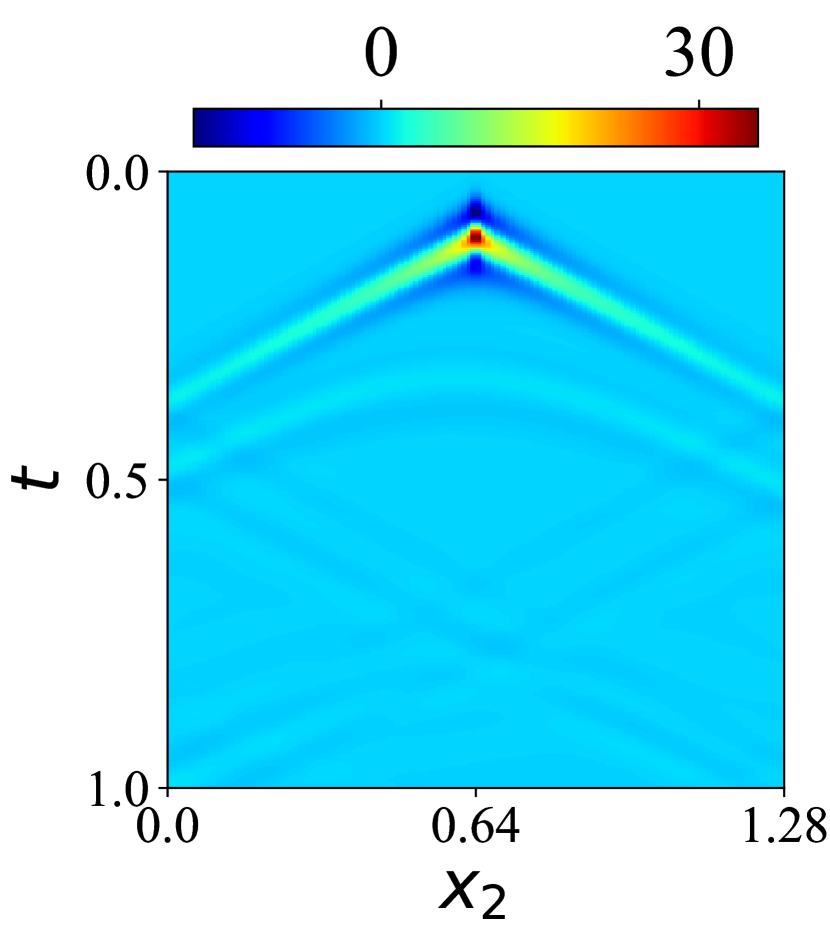
(b) Measurements at receivers

Figure 7: Wave propagation via piece-wise square slowness and oval-shaped interface.

Oval-shaped square slowness. In the first problem, the source was placed at a depth of 50m and horizontally in the middle. The receivers were positioned at a depth of 20m. The domain was partitioned into two regions, with $m({\bf x})$ being the same within each region. See Fig. 7 of the Appendix for an example and the surveyed data by the receivers. The interface is an oval, defined by its center $(x_{1c},x_{2c})$, and two radii $w$ and $h$. We sampled $x_{1c},x_{2c}\sim\mathcal{U}(\frac{1}{4}\times 1.28\,\mathrm{km},\frac{3}{4}\times 1.28\,\mathrm{km})$, and $w,h\sim\mathcal{U}(\frac{1}{10}\times 1.28\,\mathrm{km},\frac{1}{5}\times 1.28\,\mathrm{km})$. Inside the ellipse, we set the value of $m$ to 3, while the outside the ellipse, we sampled the value from ${\mathcal{U}}(1,2)$. We used the Devito library (https://github.com/devitocodes/devito) to simulate the receivers’ measurements. The square slowness was generated on a $128\times 128$ grid, and the measurements were computed at $614$ time steps. The data was then downsampled to a $64\times 64$ grid and $62$ time steps.

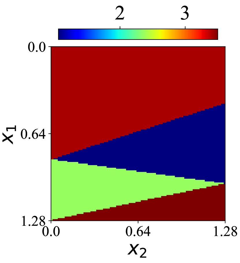
(a) Square slowness

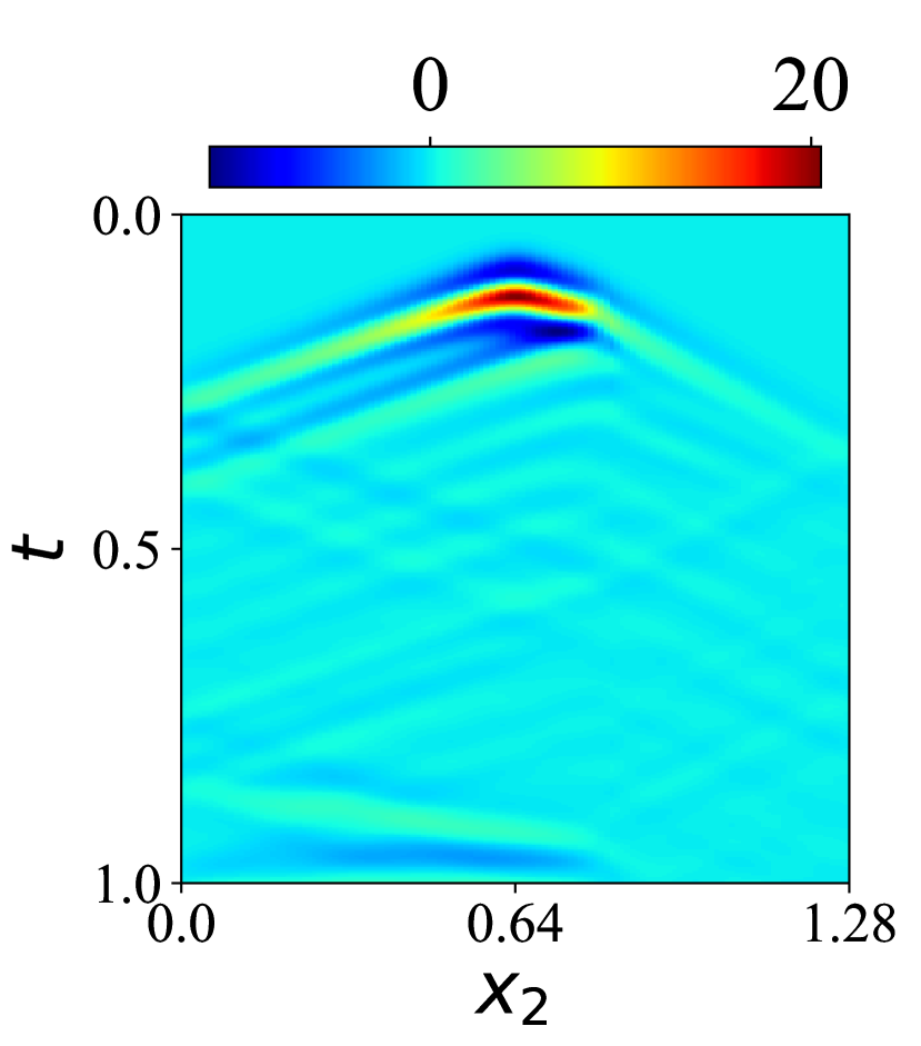
(b) Measurements at receivers

Figure 8: Wave propagation via piece-wise square slowness and Z-shaped interface.

Z-shaped square slowness. In the second problem, the source was positioned at a depth of 80m (still horizontally in the middle). The domain was divided into four regions, with the interfaces between these regions forming a z-shape. The values of $m({\bf x})$ inside each region are identical; see Fig. 8 of the Appendix for an example. We represented the end points of these interfaces by $(1.28\,\mathrm{km},0)$,$(z_{1},1.28\,\mathrm{km})$, $(z_{2},0)$, and $(z_{3},1.28\,\mathrm{km})$, where $z_{1}\sim U(\frac{3}{4}\times 1.28\,\mathrm{km},1.28\,\mathrm{km})$, $z_{2}\sim U(\frac{1}{2}\times 1.28\,\mathrm{km},\frac{3}{4}\times 1.28\,\mathrm{km})$, and $z_{3}\sim\mathcal{U}(\frac{1}{4}\times 1.28\,\mathrm{km},\frac{1}{2}\times 1.28\,\mathrm{km})$. We set $m=3.5$ in the bottom region, and sampled the value of $m({\bf x})$ for each of the other three regions from ${\mathcal{U}}(0.5,3.5)$. The receivers’ measurements were computed at 573 time steps with spatial resolution $128$, and then downsampled at 58 steps with spatial resolution 64.

For both problems, we used 400 examples for training and 100 for testing. Similarly to Sec. 5.1, we also injected 10% and 20% Gaussian white noises into the training datasets to evaluate the robustness of our method.

5.3 Navier-Stoke Equation

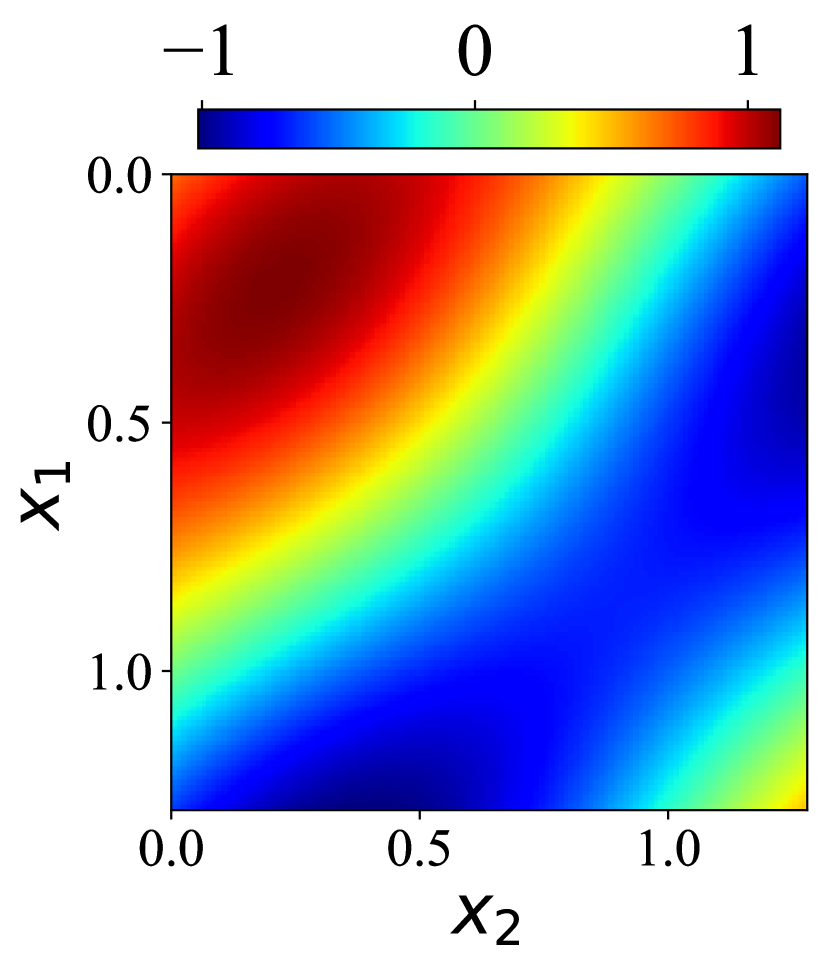
(a) Initial condition

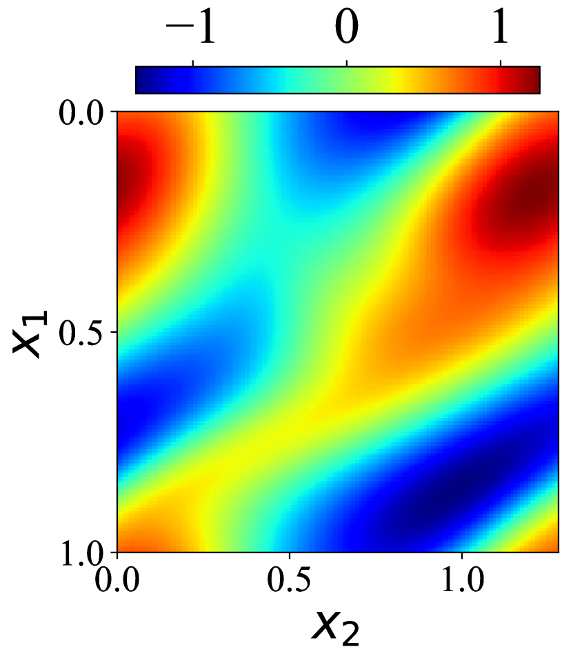
(b) Solution at $t=10$

Figure 9: Solution of NS equation.

Third, we considered the 2D Navier-Stokes (NS) equation as used in (Li et al., 2020c). The solution represents the vorticity of a viscous, incompressible fluid within the spatial domain ${\bf x}=(x_{1},x_{2})\in[0,1]^{2}$. The viscosity was set to $10^{-3}$. In the forward scenario, we aim to predict the vorticity at time $t=10$ from the initial condition. Correspondingly, in the inverse scenario, the goal is to reconstruct the initial condition $\omega_{0}$ from the observed vorticity at $t=10$. We generated the initial condition by $\omega_{0}(x_{1},x_{2})=\sum_{i=1}^{2}\sum_{j=1}^{2}q_{ij}\sin(\alpha_{i}\pi(x_{1}+c_{j}))\cdot q_{ij}\cos(\alpha_{i}\pi(x_{2}+c_{j}))$, where $\alpha_{i}\sim\mathcal{U}(0.5,1),c_{j}\sim\mathcal{U}(0,1)$, and $q_{ij}\sim\mathcal{U}(-1,1)$. An example is given by Appendix Fig. 9. For each experiment, we used $1000$ training examples and $200$ test examples. Again, we performed additional tests by injecting 10% and 20% noises into both the training input and output function samples.

Benchmark	0%				10%				20%
	iFNO	IDON	FNO		iFNO	iDON	FNO		iFNO	iDON	FNO
D-LINE	0.0358	0.384	0.0958		0.0532	0.407	0.111		0.0830	0.486	0.142
D-CURV	0.0370	7.18	0.233		0.0611	5.48	0.354		0.0635	5.66	0.508
W-OVAL	0.0850	0.319	0.318		0.101	0.320	0.318		0.105	0.321	0.318
W-Z	0.300	0.984	0.964		0.314	0.980	0.973		0.372	0.982	0.975
NS	0.0213	0.341	0.0377		0.0315	0.341	0.150		0.0431	0.343	0.160

(a) Forward

Benchmark	0%					10%					20%
	iFNO	iDON	NIO	FNO		iFNO	iDON	NIO	FNO		iFNO	iDON	NIO	FNO
D-LINE	0.0581	0.234	0.123	0.119		0.0947	0.248	0.187	0.193		0.112	0.451	0.202	0.195
D-CURV	0.0564	0.212	0.0824	0.0835		0.0765	0.198	0.195	0.131		0.0984	0.218	0.222	0.176
W-OVAL	0.0608	0.146	0.0935	0.128		0.0854	0.149	0.113	0.130		0.103	0.152	0.125	0.146
W-Z	0.163	0.267	0.221	0.250		0.178	0.291	0.229	0.258		0.187	0.311	0.234	0.264
NS	0.0614	0.113	0.0739	0.105		0.0757	0.122	0.107	0.283		0.0853	0.137	0.119	0.310

(b) Inverse

Table 1: Relative $L_{2}$ error on each task, where “D-” and “W-” indicate Darcy flow and wave propagation, respectively, “LINE”, “CURV”, “OVAL”, and “Z” represent linear, curved, oval, and z-shaped interfaces, respectively as explained in Section 5.1 and 5.2, and $0\%,10\%,20\%$ indicate the noise level in the training data.

5.4 Results and Analysis

We compared the proposed iFNO with the invertible Deep Operator Net (iDON) (Kaltenbach et al., 2022), the neural inverse operator (NIO) (Molinaro et al., 2023), and the standard FNO. We evaluated all the methods in both forward and inverse tasks, except for NIO, which is exclusively designed for inverse prediction. We implemented iFNO with PyTorch and used the original implementation of all the competing methods. For a fair comparison, we meticulously tuned each method to achieve the optimal performance to the best of our ability. The details of the hyperparameter choice and tuning can be found in Section A of the Appendix.

Predictive performance. The relative $L_{2}$ error of all the methods is reported in Table 1. We can see that in both forward and inverse problems, iFNO consistently outperforms the competing methods by a large margin. Notably, iFNO greatly surpasses the two FNO models, one exclusively trained for forward prediction, and the other exclusively for inverse prediction. Meanwhile, the size of iFNO is considerably smaller than the combined size of the FNO models. For instance, on W-Z and NS, iFNO reduces parameters by 80.6% and 66.7% compared to the two FNO models. This highlights that our co-learning approach, utilizing a shared NO architecture, not only enhances the performance in both forward and inverse tasks but also significantly reduces the memory cost in training. We present the model size of all the methods on each benchmark in Table 2. Due to the invertible architecture in the branch net, iDON must maintain each layer width to be the same as the input dimension, resulting in a large number of model parameters. However, despite its extensive model size, iDON often exhibits lower prediction accuracy as compared to the other methods. This suggests that the sizable model might pose challenges for effective learning, not to mention much more training cost. See the running time of each method in Appendix Table 4.

Point-wise error and prediction uncertainty. For a detailed assessment, we performed a fine-grained evaluation by visualizing the point-wise prediction error of iFNO in ten randomly selected instances within the inverse scenario. Additionally, we investigated prediction uncertainty by sampling 500 predictions from the VAE component (refer to (9)) for each instance. The standard deviation of these predictions at each location is then calculated. The point-wise error is determined based on the predictive mean of the Gauss encoder. The outcomes are depicted in Fig. 2.

Overall, it is evident that the error grows as the noise level increases, mirroring a similar trend in prediction uncertainty. For problems involving Darcy flow and wave propagation (the first eight instances), the point-wise error is predominantly concentrated at the interfaces between different regions. This pattern is echoed in the prediction uncertainty of iFNO, with the standard deviation being significantly larger at the interfaces compared to other locations. These findings are not only intriguing but also intuitively reasonable. Specifically, since the ground-truth permeability and square slowness (that we aim to recover) are identical within the same region but distinct across different regions, predicting values within each region becomes relatively easier, resulting in lower uncertainty (higher confidence). Conversely, at the interfaces, where the ground-truth undergoes abrupt changes, predicting values becomes more challenging, leading to an increase in prediction uncertainty to reflect these challenges (lower confidence).

In the initial condition recovery problem (the last two instances), the point-wise prediction error is primarily concentrated near the boundary of the domain. Correspondingly, the predictive standard deviation of iFNO is larger near the boundary. As the noise level increases, the error at the boundary also increases, along with the calibration of uncertainty.

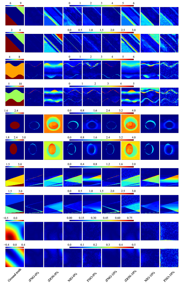
Figure 3: Point-wise error of inverse prediction, where “-0%” and “-10%” indicate the noise level in the training data.

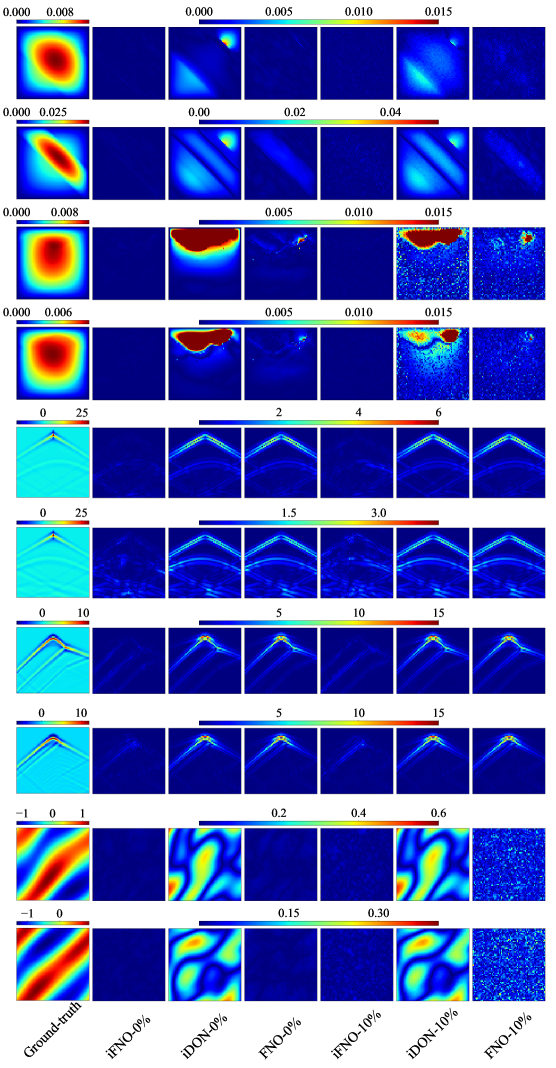
Figure 4: Point-wise error of forward prediction, where “-0%” and “-10%” indicate the noise level in the training data.

The comparison of point-wise errors with the competing methods is presented in Fig.3 and 4 of the Appendix, encompassing both forward and inverse predictions. The results reveal that competing methods frequently manifest significantly larger errors in various local regions, as illustrated by instances such as iDON in the second and third instance, NIO in the sixth and seventh instance, and FNO in the seventh and eighth instance in Appendix Fig. 3, and iDON and FNO in nearly all the instances of Appendix Fig. 4.

The collective results affirm that iFNO not only achieves superior global accuracy but also excels in local ground-truth recovery. Furthermore, iFNO demonstrates the ability to provide reasonable uncertainty estimates, aligning with the predictive challenges encountered across various local regions.

Ablation Study. To investigate the impact of each component in iFNO, we conducted experiments to assess the model’s performance with and without the $\beta$-VAE component. Initially, we tested the model after pre-training, which is without the $\beta$-VAE component, and we subsequently compared it with the final prediction error achieved after fine-tuning. During fine-tuning, the invertible Fourier blocks and $\beta$-VAE are coupled to enhance predictive capabilities. The results are summarized in Table 3 .

Remarkably, even without the $\beta$-VAE component, our model, equipped solely with invertible Fourier blocks, has already outperformed all the competing methods in both forward and inverse prediction tasks. The incorporation of the $\beta$-VAE for fine-tuning further enhances the performance in both scenarios. This suggests that not only does the $\beta$-VAE contribute to uncertainty calibration, but the latent structure captured by the VAE also plays a crucial role in improving both forward and inverse predictions.

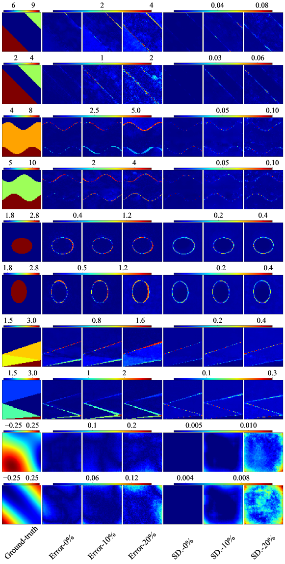
Figure 2: iFNO point-wise inverse prediction error and predictive standard deviation, denoted by “Error” and “SD” respectively followed with noise levels in training data.

	iFNO	IDON	NIO	FNO
D-LINE	13M	193M	5M	18M
D-CURV	15M	193M	5M	18M
W-OVAL	4M	193M	5M	5M
W-Z	6M	193M	4M	31M
NS	12M	193M	6M	36M

Table 2: The parameter count for each method.

Benchmark	Forward		Inverse
	Pre-train	Fine-tune	Pre-train	Fine-tune
0% noise
D-LINE	0.0391	0.0358	0.0649	0.0581
D-CURV	0.0443	0.0370	0.0585	0.0564
W-OVAL	0.124	0.0850	0.0668	0.0608
W-Z	0.300	0.300	0.1746	0.163
NS	0.0224	0.0213	0.0652	0.0614
10% noise
D-LINE	0.0546	0.0532	0.114	0.0947
D-CURY	0.0633	0.0611	0.0801	0.0765
W-OVAL	0.146	0.101	0.0886	0.0854
W-Z	0.314	0.314	0.188	0.178
NS	0.0396	0.0315	0.0913	0.0757
20% noise
Darcy1	0.0874	0.0830	0.1345	0.112
Darcy2	0.0763	0.0635	0.1024	0.0984
Wave1	0.141	0.105	0.111	0.103
Wave2	0.373	0.372	0.204	0.187
NS	0.0477	0.0431	0.102	0.0853

Table 3: Relative $L_{2}$ error of pre-training vs. fine-tuning.

6 Conclusion

We have introduced iFNO, an invertible Fourier Neural Operator designed to address both forward and inverse problems. By co-learning the bi-directional tasks within a unified architecture, iFNO not only reduces model size and memory requirements but also enhances prediction accuracy for both tasks. Additionally, iFNO demonstrates the capability to provide uncertainty calibration. Through five benchmark numerical experiments, iFNO showcases promising predictive performance.

At present, iFNO is constrained to measurement data sampled at regular grids, owing to the usage of Fourier transform. The challenge posed by irregularly sampled data can be mitigated by straightforwardly interpolating it to a regular grid. In the future, we plan to develop a more advanced approach that concurrently learns forward and inverse predictions within a latent grid space. The approach, akin to (Li et al., 2022), entails formulating a transformation that maps predictions in the latent space to the actual observational space.

A Experimental Details

All the models were trained with AdamW or the Adam optimizer with exponential decay strategy or the reducing learning rate on plateau strategy. The learning rate was chosen from $\{10^{-5},10^{-4},5\times 10^{-4},10^{-3},10^{-2}\}$. We varied the mini-batch size from {10, 20, 50}.

• iFNO. We used four invertible Fourier blocks for all the experiments. We set the lifting dimension to 64 (channel numbers). We varied the number of Fourier modes (for frequency truncation) from {8, 12, 16, 32}. The number of epochs for pre-training invertible Fourier blocks was tuned from {100, 200, 500}, and $\beta$-VAE from {200, 500, 1000}. The number of fine-tuning epochs was set from {50,100,500}. The architecture of $\beta$-VAE is the same accross all the benchmarks. We employed a Gaussian encoder that includes five convolutional layers with 32, 64, 128, 256 and 512 channels respectively. The decoder first applies five transposed convolutional layers to sequntially reduce the number of channels to 512, 256, 128, 64, and 32. Then a transposed convolutional layer (with 32 output channels) and another convolutional layer (with one output channel) are applied to produce the prediction of ${\bf f}$. We set $\beta=0.01$ for all the benchmarks except for Darcy flow, we set $\beta=10^{-6}$.

• FNO. We used the original FNO implementation (https://github.com/neuraloperator/neuraloperator). To ensure convergence, we set the number of training epochs to 1000. The lifting dimension was chosen from $\{32,64,128\}$. The number of Fourier modes was tuned from $\{8,12,16,32\}$. The number of Fourier layers was selected from $\{2,3,4\}$.

• iDON. We used the Jax implementation of iDON from the authors (https://github.com/pkmtum/Semi-supervised_Invertible_Neural_Operators/tree/main). The number of training epochs was set to 1000. We varied the number of layers for the branch net and trunk set from {3, 4, 5}. Note that to ensure invertibility, the width of the branch net must be set to the dimension of the (discretized) input function. For instance, if the input function is sampled on a $64\times 64$ grid, the width of the branch net will be $4096$. The width of the trunk net is set to be the width of the branch net. For a fair comparison, only the forward and backward supervised loss terms were retained for training.

• NIO. We used the PyTorch implementation from the authors (https://github.com/mroberto166/nio). We employed 1000 training epochs. NIO used convolution layers for the branch net of the deepONet module. We tuned the number of convolution layers from {6,8,10}, and kernel size from {3,5}, and padding from {1,3}. The stride is fixed to 2. For the trunk net, we tuned the number of layers from $\{2,3,4\}$, and the layer width from $\{32,64,128,256\}$. For the FNO component, we varied the number of Fourier layers from $\{1,2,3\}$, lifting dimension from $\{32,64,128\}$, and the number of Fourier modes from $\{8,12,16,32\}$.

Benchmark	iFNO	IDON	NIO	FNO
D-LINE	17 mins	5.7 hours	5 mins	11 mins
D-CURV	68 mins	15.3 hours	10 mins	31 mins
W-OVAL	13 mins	7.8 hours	5 mins	20 mins
W-Z	22 mins	7.9 hours	4 mins	15 mins
NS	50 mins	36.8 hours	13 mins	40 mins

Table 4: Running time of each method, measured at a Linux workstation with NVIDIA GeForce RTX 3090.

References

- Bhan et al. (2023) Luke Bhan, Yuanyuan Shi, and Miroslav Krstic. Operator learning for nonlinear adaptive control. In Learning for Dynamics and Control Conference, pages 346–357. PMLR, 2023.
- Dinh et al. (2016) Laurent Dinh, Jascha Sohl-Dickstein, and Samy Bengio. Density estimation using real nvp. arXiv preprint arXiv:1605.08803, 2016.
- Gupta et al. (2021) Gaurav Gupta, Xiongye Xiao, and Paul Bogdan. Multiwavelet-based operator learning for differential equations. Advances in neural information processing systems, 34:24048–24062, 2021.
- Higgins et al. (2016) Irina Higgins, Loic Matthey, Arka Pal, Christopher Burgess, Xavier Glorot, Matthew Botvinick, Shakir Mohamed, and Alexander Lerchner. beta-vae: Learning basic visual concepts with a constrained variational framework. In International conference on learning representations, 2016.
- Kaltenbach et al. (2022) Sebastian Kaltenbach, Paris Perdikaris, and Phaedon-Stelios Koutsourelakis. Semi-supervised invertible deeponets for bayesian inverse problems. arXiv preprint arXiv:2209.02772, 2022.
- Kaltenbach et al. (2023) Sebastian Kaltenbach, Paris Perdikaris, and Phaedon-Stelios Koutsourelakis. Semi-supervised invertible neural operators for bayesian inverse problems. Computational Mechanics, pages 1–20, 2023.
- Kingma and Welling (2013) Diederik P Kingma and Max Welling. Auto-encoding variational bayes. arXiv preprint arXiv:1312.6114, 2013.
- Kovachki et al. (2023) Nikola B Kovachki, Zongyi Li, Burigede Liu, Kamyar Azizzadenesheli, Kaushik Bhattacharya, Andrew M Stuart, and Anima Anandkumar. Neural operator: Learning maps between function spaces with applications to pdes. J. Mach. Learn. Res., 24(89):1–97, 2023.
- Li and Shatarah (2024) Haochen Li and Mohamed Shatarah. Operator learning for urban water clarification hydrodynamics and particulate matter transport with physics-informed neural networks. Water Research, page 121123, 2024.
- Li et al. (2020a) Zongyi Li, Nikola Kovachki, Kamyar Azizzadenesheli, Burigede Liu, Kaushik Bhattacharya, Andrew Stuart, and Anima Anandkumar. Neural operator: Graph kernel network for partial differential equations. arXiv preprint arXiv:2003.03485, 2020a.
- Li et al. (2020b) Zongyi Li, Nikola Kovachki, Kamyar Azizzadenesheli, Burigede Liu, Andrew Stuart, Kaushik Bhattacharya, and Anima Anandkumar. Multipole graph neural operator for parametric partial differential equations. Advances in Neural Information Processing Systems, 33:6755–6766, 2020b.
- Li et al. (2020c) Zongyi Li, Nikola Borislavov Kovachki, Kamyar Azizzadenesheli, Kaushik Bhattacharya, Andrew Stuart, Anima Anandkumar, et al. Fourier neural operator for parametric partial differential equations. In International Conference on Learning Representations, 2020c.
- Li et al. (2022) Zongyi Li, Daniel Zhengyu Huang, Burigede Liu, and Anima Anandkumar. Fourier neural operator with learned deformations for PDEs on general geometries. arXiv preprint arXiv:2207.05209, 2022.
- Liu et al. (2023) Ziyue Liu, Yixing Li, Jing Hu, Xinling Yu, Shinyu Shiau, Xin Ai, Zhiyu Zeng, and Zheng Zhang. Deepoheat: Operator learning-based ultra-fast thermal simulation in 3d-ic design. arXiv preprint arXiv:2302.12949, 2023.
- Lu et al. (2021) Lu Lu, Pengzhan Jin, Guofei Pang, Zhongqiang Zhang, and George Em Karniadakis. Learning nonlinear operators via deeponet based on the universal approximation theorem of operators. Nature machine intelligence, 3(3):218–229, 2021.
- Lu et al. (2022) Lu Lu, Xuhui Meng, Shengze Cai, Zhiping Mao, Somdatta Goswami, Zhongqiang Zhang, and George Em Karniadakis. A comprehensive and fair comparison of two neural operators (with practical extensions) based on fair data. Computer Methods in Applied Mechanics and Engineering, 393:114778, 2022.
- Molinaro et al. (2023) Roberto Molinaro, Yunan Yang, Björn Engquist, and Siddhartha Mishra. Neural inverse operators for solving pde inverse problems. arXiv preprint arXiv:2301.11167, 2023.
- Nashed and Scherzer (2002) M Zuhair Nashed and Otmar Scherzer. Inverse Problems, Image Analysis, and Medical Imaging: AMS Special Session on Interaction of Inverse Problems and Image Analysis, January 10-13, 2001, New Orleans, Louisiana, volume 313. American Mathematical Soc., 2002.
- Pathak et al. (2022) Jaideep Pathak, Shashank Subramanian, Peter Harrington, Sanjeev Raja, Ashesh Chattopadhyay, Morteza Mardani, Thorsten Kurth, David Hall, Zongyi Li, Kamyar Azizzadenesheli, et al. Fourcastnet: A global data-driven high-resolution weather model using adaptive fourier neural operators. arXiv preprint arXiv:2202.11214, 2022.
- Pfaff et al. (2020) Tobias Pfaff, Meire Fortunato, Alvaro Sanchez-Gonzalez, and Peter W Battaglia. Learning mesh-based simulation with graph networks. arXiv preprint arXiv:2010.03409, 2020.
- Seidman et al. (2022) Jacob Seidman, Georgios Kissas, Paris Perdikaris, and George J Pappas. Nomad: Nonlinear manifold decoders for operator learning. Advances in Neural Information Processing Systems, 35:5601–5613, 2022.
- Stuart (2010) Andrew M Stuart. Inverse problems: a Bayesian perspective. Acta numerica, 19:451–559, 2010.
- Tanaka and Dulikravich (1998) Masataka Tanaka and George S Dulikravich. Inverse problems in engineering mechanics. Elsevier, 1998.
- Yilmaz (2001) Öz Yilmaz. Seismic data analysis: Processing, inversion, and interpretation of seismic data. Society of exploration geophysicists, 2001.
- Zhao et al. (2022) Qingqing Zhao, David B Lindell, and Gordon Wetzstein. Learning to solve pde-constrained inverse problems with graph networks. arXiv preprint arXiv:2206.00711, 2022.