The Gerber-Shiu Expected Discounted Penalty Function: An Application to Poverty Trapping

Abstract

In this article, we consider a risk process with deterministic growth and prorated losses to model the capital of a household. Our work focuses on the analysis of the trapping time of such a process, where trapping occurs when a household’s capital level falls into the poverty area, a region from which it is difficult to escape without external help. A function analogous to the classical Gerber-Shiu expected discounted penalty function is introduced, which incorporates information on the trapping time, the capital surplus immediately before trapping and the capital deficit at trapping. Given that the remaining proportion of capital upon experiencing a capital loss is $Beta(\alpha,1)-$distributed, closed-form expressions are obtained for quantities typically studied in classical risk theory, including the Laplace transform of the trapping time and the distribution of the capital deficit at trapping. In particular, we derive a model belonging to the generalised beta (GB) distribution family that describes the distribution of the capital deficit at trapping given that trapping occurs. Affinities between the capital deficit at trapping and a class of poverty measures, known as the Foster-Greer-Thorbecke (FGT) index, are presented. The versatility of this model to estimate FGT indices is assessed using household microdata from Burkina Faso’s Enquête Multisectorielle Continue (EMC) 2014.

Keywords— Foster–Greer–Thorbecke (FGT) index; Gerber-Shiu function; poverty traps; poverty measures; risk process.

1 Introduction

Recently, risk theory has proven to be a powerful tool to analyse a household’s infinite-time trapping probability (the probability of a household’s capital falling into the area of poverty at some point in time) (see, for instance, Kovacevic and Pflug (2011), Flores-Contró et al. (2021) and Henshaw et al. (2023)). The classical risk process, also known as the Cramér-Lundberg model, which was introduced by Cramér and Lundberg at the beginning of the last century (Lundberg, 1903, 1926; Cramér, 1930), has been adapted to better portray the capital of a household. For example, in Kovacevic and Pflug (2011), Flores-Contró et al. (2021) and Henshaw et al. (2023), only the surplus of a household’s current capital above a critical capital level (or poverty line) grows exponentially, unlike the linear premium income for an insurer’s surplus in the Cramér-Lundberg model. Moreover, Kovacevic and Pflug (2011) and Henshaw et al. (2023) consider household capital losses as a proportion of the accumulated capital, yielding absolute losses that are serially correlated with each other and with the inter-arrival times of loss events. In contrast, losses in the Cramér-Lundberg model are given by a sequence of i.i.d. claim sizes and are subtracted from the insurer’s surplus rather than prorated. Similar models with prorated jumps have been studied outside the actuarial science domain (see Altman et al. (2002), Altman et al. (2005) and Löpker and Van Leeuwaarden (2008), for an application of this type of model on data transmission over the internet; Eliazar and Klafter (2004) and Eliazar and Klafter (2006) for their use in representing the behaviour of physical systems with a growth-collapse pattern; and Derfel et al. (2012) for the adoption of these processes to modelling the division and growth of cell-populations).

This article examines the household capital process with proportional losses originally introduced in Kovacevic and Pflug (2011) and subsequently studied in Azaïs and Genadot (2015) and Henshaw et al. (2023). Previous work on this capital process focuses solely on studying the infinite-time trapping probability. Indeed, Kovacevic and Pflug (2011) and Azaïs and Genadot (2015) use numerical methods to estimate the trapping probability, without aiming to find an analytical solution for the probability. However, as stated by Asmussen and Albrecher (2010), the ideal situation in risk theory is to derive closed-form solutions for trapping probabilities. To this end, Henshaw et al. (2023) apply Laplace transform techniques to solve the infinitesimal generator of the household’s capital risk process and obtain a closed-form expression for the infinite-time trapping probability under the assumption of $Beta(\alpha,1)-$distributed remaining proportions of capital.

Although the infinite-time trapping probability is a very important indicator for studying poverty dynamics, policy makers and other stakeholders may need additional information on other quantities to fully understand a household’s transition into poverty. A clear example of a quantity of interest is the income short-fall (or income gap), which is defined as the absolute value of the difference between a poor household’s income (or consumption) and some poverty line. A household’s income short-fall serves as key component in a number of poverty measures (see, for instance, Sen (1976), where a simple poverty measure, the income-gap ratio, assesses the percentage of household’s mean income short-fall from the poverty line and Foster et al. (1984), where the well-known Foster-Greer-Thorbecke (FGT) index weights the income gaps of the poor to estimate the aggregate poverty of an economic entity). The primary objective of incorporating household levels of income short-fall in poverty measures is the elimination of certain measurement issues. That is, numerous poverty measures, such as the head-count index, which calculates the proportion of the population living below the poverty line and has been considered as one of the most common indices for measuring poverty since the first studies of poverty were conducted (see, Booth (1889) and Rowntree (1901)), ignore the depth of poverty and the distribution of income among the poor, making them deficient as poverty indicators (Sen, 1976). Consequently, this underlines the importance of exploring additional quantities such as a household’s income short-fall.

Apart from facilitating the study of the infinite-time trapping probability, classical risk theory provides additional tools that allow the examination of other quantities of interest, such as a household’s income short-fall at the trapping time (the time at which a household’s capital falls into the area of poverty), thus granting a much deeper understanding of a household’s transition into poverty. In particular, the Gerber-Shiu expected discounted penalty function, which was originally introduced by Gerber and Shiu (1998), gives information about three quantities: the time of ruin, the deficit at ruin, and the surplus prior to ruin, corresponding to the first time an insurer’s surplus becomes negative, the undershoot and the overshoot of the insurer’s surplus at ruin, respectively. These three random variables play an important role within the risk management strategy of an insurance company. For instance, risk measures such as the Value-at-Risk and the Tail-Value-at-Risk have a close link with the deficit at ruin, while from a monitoring perspective, the surplus prior to ruin could be thought of as an early warning signal for the insurance company. The (ruin) time at which any such event takes place is then of critical importance (Landriault and Willmot, 2009). Extensive literature on these variables exists for the Cramér-Lundberg model and its variations (see, for example, Gerber and Shiu (1997), Gerber and Shiu (1998), Lin and Willmot (1999), Lin and Willmot (2000), Chiu and Yin (2003), Landriault and Willmot (2009) and references therein).

Certainly, a household’s trapping time can be thought of as the ruin time of an insurer, while the capital surplus prior to trapping and the capital deficit at trapping are analogous to the insurer’s surplus prior to ruin and the deficit at ruin, respectively. Therefore, the Gerber-Shiu expected discounted penalty function can be applied to study these quantities. Recently, for example, Flores-Contró et al. (2021) emloyed the Gerber-Shiu expected discounted penalty function to study the distribution of the trapping time of a household’s capital risk process with deterministic growth and $Exp(\alpha)-$distributed losses. Using classical risk theory techniques, Flores-Contró et al. (2021) also assess how the introduction of an insurance policy alters the distribution of the trapping time. Kovacevic and Semmler (2021) have also recently highlighted the importance of studying such trapping times to optimise the retention rates of insurance policies purchased by households. In this article, for the household capital process with proportional losses, we obtain closed-form expressions for the Gerber-Shiu expected discounted penalty function under the assumption of $Beta(\alpha,1)-$distributed remaining proportions of capital. Thus, the first contribution of this article lies in the derivation of analytical equations for the Gerber-Shiu expected discounted penalty function, which to the best of our knowledge, have not been previously obtained for this particular risk process.

Given the importance of the income short-fall and its key role in widely used poverty measures, the second contribution of this paper lies in obtaining a compelling microeconomic foundation, which emerges from the derivation of the Gerber-Shiu expected discounted penalty function for the household capital process, to model the distribution of the income short-fall. This is particularly important as parametric estimation of income distributions has long been used to model income since the introduction of the Pareto (1967) law. One of the main advantages of parametric estimation of income distributions is that explicit formulas, as functions of the parameters of the theoretical income distribution, are available to measure poverty and inequality. This allows, for example, to further interpret the shape parameters of the theoretical income distribution, as well as to carry out sensitivity analyses of poverty measures to variations in the shape parameters (Graf and Nedyalkova, 2014). In economics, it is well-known that the processes of income generation and distribution must be connected, underpinned by a microeconomic foundation, to the functional form of any model that adequately represents the distribution of personal income (Callealta Barroso et al., 2020). Our results reveal that the distribution of a household’s income short-fall belongs to the generalised beta (GB) distribution family, a group of models that have been widely used in economics for modelling income.

To assess the validity of our results, we fit the derived GB model to household microdata from Burkina Faso’s Enquête Multisectorielle Continue (EMC) 2014. Poverty measures are estimated using both the observed income short-fall data and the fitted theoretical income short-fall distribution. Goodness-of-fit tests and comparisons between theoretical and empirical poverty measures suggest that risk theory is a promising theoretical framework for studying poverty dynamics. That is, by appropriately adapting the classical Cramér-Lundberg model to better portray a household’s  capital, risk theory provides a vast framework with a diverse set of tools to explore. The application of risk theory techniques to study poverty dynamics is just beginning and its potential is yet to be discovered.

The remainder of the article is organised as follows. In Section 2, we introduce the capital of a household and its connection with the Cramér-Lundberg model. Section 3 provides a brief discussion on the GB distribution family and its application in economics for modelling income. In Section 4, the trapping time and the Gerber-Shiu expected discounted penalty function are defined. Moreover, an Integro-Differential Equation (IDE) for the Gerber-Shiu expected discounted penalty function is also derived. We obtain in Section 4.1 a closed-form expression for the Laplace transform of the trapping time when the remaining proportion of capital is $Beta(\alpha,1)-$distributed. Apart from characterising uniquely the probability distribution of the trapping time, Section 4.1 also shows how the Laplace transform of the trapping time can be applied to estimate other quantities of interest such as the expected trapping time. Likewise, Section 4.2 studies the capital deficit at trapping by means of the Gerber-Shiu expected discounted penalty function for $Beta(\alpha,1)-$distributed remaining proportions of capital and shows that the distribution of the capital deficit at trapping given that trapping occurs is described by a model belonging to the GB distribution family. Section 5 introduces the FGT index in more detail and discusses affinities between the index and the capital deficit at trapping. Built on Sections 4.2 and 5, a GB distribution is fitted to household microdata from Burkina Faso’s Enquête Multisectorielle Continue (EMC) 2014 in Section 6. In addition, FGT indices are estimated using the fitted distribution. To evaluate the adequacy of the model, empirical values of the poverty measures are compared with theoretical estimates and goodness-of-fit tests are assessed. Lastly, concluding remarks are discussed in Section 7.

2 The Capital of a Household

In classical risk theory, the insurance risk process with deterministic investment $(U_{t})_{t\geq 0}$ is given by

$$U_{t}=u+pt+\nu\int_{0}^{t}U_{s}\,ds-\sum_{i=1}^{P_{t}}Y_{i},$$ (2.1)

where $u=U_{0}\geq 0$ is the insurer’s initial surplus, $p$ is the incoming premium rate per unit time, $\nu$ is the risk-free interest rate, $(P_{t})_{t\geq 0}$ is a Poisson process with intensity $\mathcal{I}$ counting the number of claims in the time interval $[0,t]$ and $(Y_{i})_{i=1}^{\infty}$ is a sequence of i.i.d. claim sizes with distribution function $G_{Y}$. Initially introduced by Segerdahl (1942), this model was subsequently studied by Harrison (1977) and Sundt and Teugels (1995). Readers may wish to consult Paulsen (1998) for a detailed literature review on this model.

Adopting traditional risk theory techniques, this article examines ideas proposed in Kovacevic and Pflug (2011). In particular, we study a household’s capital process $(X_{t})_{t\geq 0}$ with a deterministic exponential growth and multiplicative capital loss (collapse) structure. The process grows exponentially with a rate $r>0$, which incorporates household rates of consumption ($0<a<1$), income generation ($0<b$) and investment or savings ($0<c<1$), above a critical capital (or poverty line) $x^{*}>0$ whereas below this critical threshold it remains constant. At time $T_{i}$, the $i\text{th}$ capital loss event time of a Poisson process $(N_{t})_{t\geq 0}$ with parameter $\lambda$, the capital process jumps (downwards) to $Z_{i}\cdot X_{T_{i}}$, where $(Z_{i})_{i=1}^{\infty}$ is a sequence of i.i.d. random variables with distribution function $G_{Z}$ supported in $[0,1]$, independent of the process $N_{t}$, representing the proportions of remaining capital after each loss event. Therefore, a household’s capital process in between jumps is given by

$$X_{t}=\begin{cases}\left(X_{T_{i-1}}-x^{*}\right)e^{r\left(t-T_{i-1}\right)}+x^{*}&\textit{ if }X_{T_{i-1}}>x^{*},\\ X_{T_{i-1}}&\textit{otherwise},\end{cases}$$ (2.2)

for $T_{i-1}\leq t<T_{i}$ and $T_{0}=0$. On the other hand, at the jump times $t=T_{i}$, the capital process is given by

$$X_{T_{i}}=\begin{cases}\left[\left(X_{T_{i-1}}-x^{*}\right)e^{r\left(T_{i}-T_{i-1}\right)}+x^{*}\right]\cdot Z_{i}&\textit{ if }X_{T_{i-1}}>x^{*},\\ X_{T_{i-1}}\cdot Z_{i}&\textit{otherwise}.\end{cases}$$ (2.3)

The stochastic process $(X_{t})_{t\geq 0}$ is a piecewise-determinsitic Markov process (Davis, 1984, 1993) and its infinitesimal generator is given by

$$(\mathcal{A}f)(x)=r(x-x^{*})f^{\prime}(x)+\lambda\int_{0}^{1}\left[f(x\cdot z)-f(x)\right]\mathrm{d}G_{Z}(z),\qquad x\geq x^{*}.$$ (2.4)

There exist many similarities between the household capital process and other well-known risk processes. For instance, observe that when $p=0$, the insurance risk process (2.1) is equivalent to the household capital process above the critical capital $x^{*}=0$ with claim losses subtracted from the insurer’s surplus rather than prorated. Furthermore, taking the logarithm of a discretised version of the household capital process, that is, setting the critical capital $x^{*}=0$ and taking the logarithm of (2.3), yields a version of the classical risk process (see, for instance, Kovacevic and Pflug (2011) and Henshaw et al. (2023)), also known as the Cramér-Lundberg model, introduced by Cramér and Lundberg at the beginning of the last century (Lundberg, 1903, 1926; Cramér, 1930). This model considers linear premium income for the surplus of an insurance company with losses given by a sequence of i.i.d. claim sizes. Clearly, the Cramér-Lundberg model could also be seen as a particular case of the risk process (2.1) with $\nu=0$. Despite these resemblances, there are also a number of discrepancies between the household capital process and those commonly studied in the actuarial science literature. Firstly, only the surplus of a household’s current capital above the critical capital grows exponentially. Secondly, household losses are defined as a proportion of the accumulated capital, yielding absolute losses that are serially correlated with each other and with the inter-arrival times of loss events (Kovacevic and Pflug, 2011; Henshaw et al., 2023).

3 The Generalised Beta Distribution Family

The probability density function (pdf) of the generalised beta (GB) distribution family is given by

$$GB(y;a,b,c,p,q)=\frac{|a|y^{ap-1}\left(1-(1-c)(y/b)^{a}\right)^{q-1}}{b^{ap}\mathrm{~{}B}(p,q)\left(1+c(y/b)^{a}\right)^{p+q}}\qquad\textit{ for }\qquad 0<y^{a}<\frac{b^{a}}{1-c},$$ (3.1)

and zero otherwise, where $0\leq c\leq 1$; $b,p,q>0$; and $B(p,q)=\int_{0}^{1}t^{p-1}(1-t)^{q-1}dt$ denotes the beta function (see, for instance, equation (6.2.1) from Abramowitz and Stegun (1972)). The GB includes other distributions as special or limiting cases (see, for example, McDonald and Xu (1995)). In particular, the beta of the first kind (B1), with pdf

$$B1(y;b,p,q):=GB(y;a=1,b,c=0,p,q)=\frac{y^{p-1}(b-y)^{q-1}}{b^{p+q-1}B(p,q)}\qquad\textit{ for }\qquad 0<y<b,$$ (3.2)

arises as the model that describes the distribution of a household’s income short-fall, for the particular case in which the remaining proportions of capital $Z_{i}$ are $Beta(\alpha,1)-$distributed. Indeed, the results obtained in Section 4.2 validate the adequacy of the B1 distribution as a model of income distribution and, in particular, as a model for the distribution of the income short-fall. Thurow (1970) was the first to adopt the standard beta distribution ($Beta(p,q):=B1(y;b=1,p,q)$) to analyse factors contributing to income inequality among whites and blacks. One of the main advantages of the beta distribution is that it includes the gamma distribution as a limiting case and therefore provides at least as good a fit as the gamma. This is an important feature, especially since the gamma distribution has also been considered to model income distribution (Salem and Mount, 1974). In the 1980s, seeking to improve the goodness of fit of the two-parameter standard beta distribution, McDonald (1984) introduced the generalized beta of the first and second kind ($GB1:=GB(y;a,b,c=0,p,q)$ and $GB2:=GB(y;a,b,c=1,p,q)$), two four-parameter distributions that nest most of the previously used models of two and three parameters as special cases or limit distributions (e.g. the Singh-Maddala distribution (Singh and Maddala, 1976)). Subsequently, McDonald and Xu (1995) introduced (3.1), a five-parameter distribution that has clearly played an important role for modelling income. In fact, many distributions (belonging or not to the GB distribution family) with a varying number of parameters have been used in the literature to model income (see Hlasny (2021) for a detailed survey).

4 When and How Households Become Poor?

Let

$$\tau_{x}:=\inf\left\{t\geq 0:X_{t}<x^{*}\mid X_{0}=x\right\}$$ (4.1)

denote the time at which a household with initial capital $x\geq x^{*}$ falls into the area of poverty (the trapping time), where $\psi(x)=\mathbb{P}(\tau_{x}<\infty)$ is the infinite-time trapping probability. To study the distribution of the trapping time, we apply the Gerber-Shiu expected discounted penalty function at ruin, a concept commonly used in actuarial science (Gerber and Shiu, 1998), such that with a force of interest $\delta\geq 0$ and initial capital $x\geq x^{*}$, we consider

$$m_{\delta}(x)=\mathbb{E}\left[w(X_{\tau^{-}_{x}}-x^{*},\mid X_{\tau_{x}}-x^{*}\mid)e^{-\delta\tau_{x}}\mathbbm{1}_{\{\tau_{x}<\infty\}}\right],$$ (4.2)

where $\mathbbm{1}_{\{A\}}$ is the indicator function of a set $A$, and $w(x_{1},x_{2})$, for $0\leq x_{1}<\infty$ and $0<x_{2}\leq x^{*}$, is a non-negative penalty function of $x_{1}$, the capital surplus prior to the trapping time, and $x_{2}$, the capital deficit at the trapping time. For more details on the so-called Gerber-Shiu risk theory, interested readers may wish to consult Kyprianou (2013). The function $m_{\delta}(x)$ is useful for deriving results in connection with joint and marginal distributions of $\tau_{x}$, $X_{\tau^{-}_{x}}-x^{*}$ and $\mid X_{\tau_{x}}-x^{*}\mid$. For example, when $\delta$ is considered as the argument, (4.2) can be viewed in terms of a Laplace transform. That is, (4.2) is the Laplace transform of the trapping time $\tau_{x}$ if one sets $w(x_{1},x_{2})=1$. Another choice, for any fixed $y$, is $w(x_{1},x_{2})=\mathbbm{1}_{\{x_{2}\leq y\}}$ for $\delta=0$, for which (4.2) leads to the distribution function of the capital deficit at trapping. It is not difficult to realise that, by appropriately choosing a penalty function $w(x_{1},x_{2})$ and force of interest $\delta$, various risk quantities can be modeled. He et al. (2023) provide a non-exhaustive list of such risk quantities. In this article, we are mainly interested in studying the Laplace transform of the trapping time and the distribution of the capital deficit at trapping. Thus, we will focus our analysis on the choices mentioned above. Following Gerber and Shiu (1998), our goal is to derive a functional equation for $m_{\delta}(x)$ by applying the law of iterated expectations to the right-hand side of (4.2).

Theorem 4.1.

Assume that the Gerber-Shiu expected discounted penalty function at trapping, $m_{\delta}(x)$, is differentiable. Then, for $x\geq x^{*}$, $m_{\delta}(x)$ satisfies the following Integro-Differential Equation (IDE)

$$\begin{split}r(x-x^{*})m_{\delta}^{\prime}(x)-(\delta+\lambda)m_{\delta}(x)+\lambda\int_{x^{*}/x}^{1}m_{\delta}(x\cdot z)dG_{Z}(z)=-\lambda A(x),\end{split}$$ (4.3)

where $A(x):=\int_{0}^{x^{*}/x}w(x-x^{*},x^{*}-x\cdot z)dG_{Z}(z)$, with boundary conditions

$$m_{\delta}(x^{*})=\frac{\lambda}{\delta+\lambda}A(x^{*})\ \ \ \text{and}\ \ \ \lim_{x\rightarrow\infty}m_{\delta}(x)=0.$$ (4.4)

Proof.

For $h>0$, consider the time interval $(0,h)$, and condition on the time $t$ and the proportion $z$ of remaining capital after the first capital loss in this time interval. Since the inter-arrival times of losses are exponentially distributed, the probability that there is no loss up to time $h$ is $e^{-\lambda h}$, and the probability that the first capital loss occurs between time $t$ and time $t+dt$ is $e^{-\lambda t}\lambda dt$. If

$$z<\frac{x^{*}}{(x-x^{*})e^{rt}+x^{*}},\hskip 56.9055pt$$ (4.5)

where $0<\frac{x^{*}}{(x-x^{*})e^{rt}+x^{*}}\leq 1$, trapping has occurred with the first loss. Hence,

$$\begin{split}m_{\delta}(x)&=e^{-(\delta+\lambda)h}m_{\delta}((x-x^{*})e^{rh}+x^{*})\\ &+\int_{0}^{h}\left[\int_{0}^{\frac{x^{*}}{(x-x^{*})e^{rt}+x^{*}}}w\left((x-x^{*})e^{rt},x^{*}-((x-x^{*})e^{rt}+x^{*})\cdot z\right)dG_{Z}(z)\right]e^{-(\delta+\lambda)t}\lambda dt\\ &+\int_{0}^{h}\left[\int_{\frac{x^{*}}{(x-x^{*})e^{rt}+x^{*}}}^{1}m_{\delta}(((x-x^{*})e^{rt}+x^{*})\cdot z)dG_{Z}(z)\right]e^{-(\delta+\lambda)t}\lambda dt.\end{split}$$ (4.6)

Differentiating (4.6) with respect to $h$ and setting $h=0$, (4.3) is obtained.

∎

4.1 The Trapping Time

As noted previously, specifying the penalty function such that $w(x_{1},x_{2})=1$, (4.2) becomes the Laplace transform of the trapping time, also interpreted as the expected present value of a unit payment due at the trapping time. Thus, equation (4.3) can then be written such that

$$\begin{split}0=r(x-x^{*})m_{\delta}^{\prime}(x)-(\delta+\lambda)m_{\delta}(x)+\lambda G_{Z}\left(\frac{x^{*}}{x}\right)+\lambda\int_{x^{*}/x}^{1}m_{\delta}(x\cdot z)dG_{Z}(z).\end{split}$$ (4.7)

Remark 4.1.

In general, it is not straightforward to obtain the solution of (4.7) for general distribution functions $G_{Z}$. Hence, throughout this article, it will be assumed that $Z_{i}\sim Beta(\alpha,1)$, case for which the distribution function is $G_{Z}(z)=z^{\alpha}$ and the pdf is $g_{Z}(z)=\alpha z^{\alpha-1}$ for $0<z<1$, where $\alpha>0$. Under this assumption, one can derive a closed-form expression for the Laplace transform of the trapping time.

Proposition 4.1.

Consider a household capital process defined as in (2.2) and (2.3), with initial capital $x\geq x^{*}$, capital growth rate $r$, intensity $\lambda>0$ and remaining proportions of capital with distribution $Beta(\alpha,1)$ where $\alpha>0$; that is, $Z_{i}\sim Beta(\alpha,1)$. The Laplace transform of the trapping time is given by

$$m_{\delta}(x)=\frac{\lambda\cdot{}_{2}F_{1}\left(b,b-c+1;b-a+1;y(x)^{-1}\right)}{(\lambda+\delta){}_{2}F_{1}\left(b,b-c+1;b-a+1;1\right)}{y(x)^{-b}},$$ (4.8)

where $\delta\geq 0$ is the force of interest for valuation, ${}_{2}F_{1}\left(\cdot\right)$ is Gauss’s Hypergeometric Function as defined in (4.14), $y(x)=\frac{x}{x^{*}}$, $a=\frac{-(\delta+\lambda-\alpha r)-\sqrt{(\delta+\lambda-\alpha r)^{2}+4r\alpha\delta}}{2r}$, $b=\frac{-(\delta+\lambda-\alpha r)+\sqrt{(\delta+\lambda-\alpha r)^{2}+4r\alpha\delta}}{2r}$ and $c=\alpha$.

Proof.

Under the assumption $Z_{i}\sim Beta(\alpha,1)$, the IDE (4.7) can be written such that

$$\begin{split}0=r(x-x^{*})m_{\delta}^{\prime}(x)-(\delta+\lambda)m_{\delta}(x)+\lambda\left(\frac{x^{*}}{x}\right)^{\alpha}+\lambda\int_{x^{*}/x}^{1}m_{\delta}(x\cdot z)\alpha z^{\alpha-1}dz.\end{split}$$ (4.9)

Applying the operator $\frac{d}{dx}$ to both sides of (4.9), together with a number of algebraic manipulations, yields to the following second order Ordinary Differential Equation (ODE)

$$\begin{split}0&=r(x^{2}-xx^{*})m_{\delta}^{\prime\prime}(x)+\left[(r(1+\alpha)-\delta-\lambda)x-r\alpha x^{*}\right]m_{\delta}^{\prime}(x)-\alpha\delta m_{\delta}(x).\end{split}$$ (4.10)

Letting $f(y):=m_{\delta}(x)$, such that $y$ is associated with the change of variable $y:=y(x)=\frac{x}{x^{*}}$, equation (4.10) reduces to Gauss’s Hypergeometric Differential Equation (Slater, 1960)

$$y(1-y)\cdot f^{\prime\prime}(y)+[c-(1+a+b)y]f^{\prime}(y)-abf(y)=0,$$ (4.11)

for $a=\frac{-(\delta+\lambda-\alpha r)-\sqrt{(\delta+\lambda-\alpha r)^{2}+4r\alpha\delta}}{2r}$, $b=\frac{-(\delta+\lambda-\alpha r)+\sqrt{(\delta+\lambda-\alpha r)^{2}+4r\alpha\delta}}{2r}$ and $c=\alpha$, with regular singular points at $y=0,1,\infty$ (corresponding to $x=0,x^{*},\infty$, respectively). A general solution of (4.11) in the neighborhood of the singular point $y=\infty$ is given by

$$f(y):=m_{\delta}(x)=A_{1}{y(x)}^{-a}{}_{2}F_{1}\left(a,a-c+1;a-b+1;{y(x)}^{-1}\right)+A_{2}{y(x)}^{-b}{}_{2}F_{1}\left(b,b-c+1;b-a+1;{y(x)}^{-1}\right),$$ (4.12)

for arbitrary constants $A_{1},A_{2}\in\mathbb{R}$ (see for example, equations (15.5.7) and (15.5.8) of Abramowitz and Stegun (1972)). Here,

$${}_{2}F_{1}(a,b;c;z)=\sum_{n=0}^{\infty}\frac{(a)_{n}(b)_{n}}{(c)_{n}}\frac{z^{n}}{n!}$$ (4.14)

is Gauss’s Hypergeometric Function (Gauss, 1866) and $(a)_{n}=\frac{\Gamma(a+n)}{\Gamma(n)}$ denotes the Pochhammer symbol (Seaborn, 1991).

To determine the constants $A_{1}$ and $A_{2}$, we use the boundary conditions at $x^{*}$ and at infinity. The boundary condition $\lim\limits_{x\to\infty}m_{\delta}(x)=0$, thus implies that $A_{1}=0$. Letting $x=x^{*}$ in (4.9) and (LABEL:TheTrappingTime-Subsection21-Equation6) yields

$$\frac{\lambda}{\lambda+\delta}=A_{2}\cdot{}_{2}F_{1}\left(b,b-c+1;b-a+1;1\right).$$ (4.15)

Hence, $A_{2}=\frac{\lambda}{(\lambda+\delta){}_{2}F_{1}\left(b,b-c+1;b-a+1;1\right)}$ and the Laplace transform of the trapping time is given by (4.8).

∎

Remark 4.2.

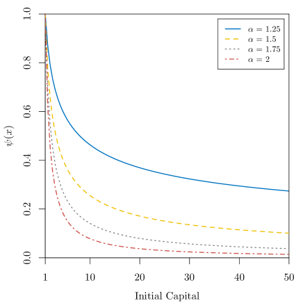
Figure 1(a) shows that the Laplace transform of the trapping time approaches the trapping probability as $\delta$ tends to zero, i.e.

$$\lim_{\delta\downarrow 0}m_{\delta}(x)=\mathbb{P}(\tau_{x}<\infty)\equiv\psi(x).$$ (4.16)

As $\delta\to 0$, (4.8) yields

$$\psi(x)=\frac{{}_{2}F_{1}\left(\alpha-\frac{\lambda}{r},1-\frac{\lambda}{r};1+\alpha-\frac{\lambda}{r};y(x)^{-1}\right)}{{}_{2}F_{1}\left(\alpha-\frac{\lambda}{r},1-\frac{\lambda}{r};1+\alpha-\frac{\lambda}{r};1\right)}y(x)^{\frac{\lambda}{r}-\alpha},$$ (4.17)

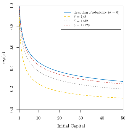
for $\alpha>\frac{\lambda}{r}$. Indeed, (4.17) was recently derived in Henshaw et al. (2023) using Laplace transform techniques. Figure 1(b) displays the trapping probability $\psi(x)$ for the capital process $X_{t}$. Note that, as mentioned in Henshaw et al. (2023), we can further simplify the expression for the trapping probability using some properties of Gauss’s Hypergeometric Function. Namely,

$${}_{2}F_{1}(a,b;c;1)=\frac{\Gamma(c)\Gamma(c-a-b)}{\Gamma(c-a)\Gamma(c-b)},\qquad\left(c\neq 0,-1,-2,...,\mathbbm{R}\left(c-a-b\right)>0\right)$$ (4.18)

(see, for example, equation (15.1.20) of Abramowitz and Stegun (1972)). Applying this relation, we obtain

$$\psi(x)=\frac{\Gamma(\alpha)\cdot{}_{2}F_{1}\left(\alpha-\frac{\lambda}{r},1-\frac{\lambda}{r};1+\alpha-\frac{\lambda}{r};y(x)^{-1}\right)}{\left(\alpha-\frac{\lambda}{r}\right)\Gamma\left(\alpha-\frac{\lambda}{r}\right)\Gamma\left(\frac{\lambda}{r}\right)}{y(x)^{\frac{\lambda}{r}-\alpha}}.$$ (4.19)

(a)

(b)

Figure 1: (a) Laplace transform $m_{\delta}(x)$ of the trapping time when $Z_{i}\sim Beta(1.25,1)$, $a=0.1$, $b=3$, $c=0.4$, $\lambda=1$, $x^{*}=1$ for $\delta=0,\frac{1}{8},\frac{1}{32},\frac{1}{128}$ (b) Trapping probability $\psi(x)$ when $Z_{i}\sim Beta(\alpha,1)$, $a=0.1$, $b=3$, $c=0.4$, $\lambda=1$, $x^{*}=1$ for $\alpha=1.25,1.5,1.75,2$.

Remark 4.3.

As an application of the Laplace transform of the trapping time, one particular quantity of interest is the expected trapping time; i.e. the expected time at which a household will fall into the area of poverty. This can be obtained by taking the derivative of $m_{\delta}(x)$:

$$\mathbb{E}\left[\tau_{x};\tau_{x}<\infty\right]=-\left.\frac{d}{d\delta}m_{\delta}(x)\right|_{\delta=0},$$ (4.20)

where $\mathbb{E}\left[\tau_{x};\tau_{x}<\infty\right]$ is equivalent to $\mathbb{E}\left[\tau_{x}\mathbbm{1}_{\{\tau_{x}<\infty\}}\right]$. As such, we differentiate Gauss’s Hypergeometric Function with respect to its first, second and third parameters. Denote

$${}_{2}F_{1}^{(a)}(a,b;c;z) \equiv\frac{d}{da}{}_{2}F_{1}(a,b;c;z),$$ (4.21)

$${}_{2}F_{1}^{(b)}(a,b;c;z) \equiv\frac{d}{db}{}_{2}F_{1}(a,b;c;z),\text{ and }$$ (4.22)

$${}_{2}F_{1}^{(c)}(a,b;c;z) \equiv\frac{d}{dc}{}_{2}F_{1}(a,b;c;z).$$ (4.23)

A closed-form expression of the aforementioned derivatives is given in terms of the Kampé de Fériet Function (Appell and Kampé De Fériet, 1926):

$$\begin{array}[]{l}F_{R,S,U}^{A,B,D}\left(\begin{array}[]{l}a_{1},\ldots,a_{A};b_{1},\ldots,b_{B};d_{1},\ldots,d_{D};\\ r_{1},\ldots,r_{R};s_{1},\ldots,s_{S};u_{1},\ldots,u_{U};\end{array}x,y\right)=\sum\limits_{m=0}^{\infty}\sum\limits_{n=0}^{\infty}\frac{\prod\limits_{j=1}^{A}\left(a_{j}\right)_{m+n}\prod\limits_{j=1}^{B}\left(b_{j}\right)_{m}\prod\limits_{j=1}^{D}\left(d_{j}\right)_{n}}{\prod\limits_{j=1}^{R}\left(r_{j}\right)_{m+n}\prod\limits_{j=1}^{S}\left(s_{j}\right)_{m}\prod\limits_{j=1}^{U}\left(u_{j}\right)_{n}}\frac{x^{m}}{m!}\frac{y^{n}}{n!}\end{array},$$ (4.27)

such that (see, for example, equations (9a) and (9b) of Ancarani and Gasaneo (2009)),

$$\begin{split}{}_{2}F_{1}^{(a)}(a,b;c;z)=\frac{zb}{c}F_{2,1,0}^{2,2,1}\left(\begin{array}[]{c}a+1,b+1;1,a;1;\\ 2,c+1;a+1;;\end{array}z,z\right),\\ \\ {}_{2}F_{1}^{(b)}(a,b;c;z)=\frac{za}{c}F_{2,1,0}^{2,2,1}\left(\begin{array}[]{c}a+1,b+1;1,b;1;\\ 2,c+1;b+1;;\end{array}z,z\right)\text{ and }\\ \\ {}_{2}F_{1}^{(c)}(a,b;c;z)=-\frac{zab}{c^{2}}F_{2,1,0}^{2,2,1}\left(\begin{array}[]{c}a+1,b+1;1,c;1;\\ 2,c+1;c+1;;\end{array}z,z\right).\end{split}$$ (4.29)

Corollary 4.1.

The expected trapping time under the household capital process defined as in (2.2) and (2.3), with initial capital $x\geq x^{*}$, capital growth rate $r$, intensity $\lambda>0$ and remaining proportions of capital with distribution $Beta(\alpha,1)$ where $\alpha>0$; that is, $Z_{i}\sim Beta(\alpha,1)$ is given by

$$\mathbb{E}\left[\tau_{x};\tau_{x}<\infty\right] =\frac{1}{r(\alpha r-\lambda)\Gamma\left(\frac{\lambda}{r}\right)^{2}\Gamma\left(\alpha-\frac{\lambda}{r}+1\right)^{2}}\Gamma(\alpha)y(x)^{\frac{\lambda}{r}-\alpha}$$ (4.30)

$$\left[\Gamma(\alpha){}_{2}F_{1}\left(1-\frac{\lambda}{r},\alpha-\frac{\lambda}{r};1+\alpha-\frac{\lambda}{r};y(x)^{-1}\right)\left((\alpha r+\lambda){}_{2}F_{1}^{(c)}\left(\alpha-\frac{\lambda}{r},1-\frac{\lambda}{r};1+\alpha-\frac{\lambda}{r};1\right)\right.\right.$$ (4.32)

$$\left.+\lambda\left({}_{2}F_{1}^{(a)}\left(\alpha-\frac{\lambda}{r},1-\frac{\lambda}{r};1+\alpha-\frac{\lambda}{r};1\right)+{}_{2}F_{1}^{(b)}\left(\alpha-\frac{\lambda}{r},1-\frac{\lambda}{r};1+\alpha-\frac{\lambda}{r};1\right)\right)\right)$$ (4.34)

$$\left.+\left(\frac{1}{\lambda}\right)\Gamma\left(\frac{\lambda}{r}\right)\Gamma\left(1+\alpha-\frac{\lambda}{r}\right)\left({}_{2}F_{1}\left(1-\frac{\lambda}{r},\alpha-\frac{\lambda}{r};1+\alpha-\frac{\lambda}{r};y(x)^{-1}\right)\left(r(\alpha r-\lambda)+\lambda^{2}\ln{\left[y(x)\right]}\right)\right.\right.$$ (4.36)

$$-\lambda\left(\left(\alpha r+\lambda\right){}_{2}F_{1}^{(c)}\left(\alpha-\frac{\lambda}{r},1-\frac{\lambda}{r};1+\alpha-\frac{\lambda}{r};y(x)^{-1}\right)\right.$$ (4.38)

$$\left.\left.\left.+\lambda\left({}_{2}F_{1}^{(a)}\left(\alpha-\frac{\lambda}{r},1-\frac{\lambda}{r};1+\alpha-\frac{\lambda}{r};y(x)^{-1}\right)+{}_{2}F_{1}^{(b)}\left(\alpha-\frac{\lambda}{r},1-\frac{\lambda}{r};1+\alpha-\frac{\lambda}{r};y(x)^{-1}\right)\right)\right)\right)\right],$$ (4.40)

where $y(x)=\frac{x}{x^{*}}$, ${}_{2}F_{1}\left(\cdot\right)$ is Gauss’s Hypergeometric Function as defined in (4.14) and ${}_{2}F_{1}^{(a)}(\cdot)$, ${}_{2}F_{1}^{(b)}(\cdot)$ and ${}_{2}F_{1}^{(c)}(\cdot)$ its derivatives with respect to the first, second and third parameters, respectively, as introduced in (4.29).

Proof.

Calculating (4.20) and using (4.29), one can derive the expected trapping time (LABEL:TheTrappingTime-Subsection21-Equation17).

∎

Figure 2: Expected trapping time $\mathbb{E}\left[\tau_{x};\tau_{x}<\infty\right]$ when $Z_{i}\sim Beta(1.5,1)$, $\lambda=1$ and $x^{*}=1$ for $r=1.0,1.1,1.2$.

Moreover, we can calculate the expected trapping time given that trapping occurs by taking the following ratio (see for example, equation (4.37) of Gerber and Shiu (1998)),

$$\begin{split}\mathbb{E}\left[\tau_{x}|\tau_{x}<\infty\right]=\frac{\mathbb{E}\left[\tau_{x};\tau_{x}<\infty\right]}{\psi(x)}.\end{split}$$ (4.42)

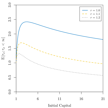
A number of expected trapping times for varying values of the capital growth rate $r$ are displayed in Figure 2. One observes that the expected trapping time is, for a fixed initial capital, typically higher when considering a lower capital growth rate $r$, which at first sight may look counter-intuitive, as a higher capital growth rate $r$ means a faster exponential growth. Nevertheless, this indicates that for high capital growth rates $r$, those trajectories that do not lead to trapping quickly, will very likely avoid it later.

4.2 The Capital Deficit at Trapping

The capital deficit at trapping is the absolute value of the difference between a household’s level of capital at the trapping time and the critical capital, i.e. the amount ${\mid X_{\tau_{x}}-x^{*}\mid}$. Specifying the penalty function such that for any fixed $y$, $w(x_{1},x_{2})=\mathbbm{1}_{\{x_{2}\leq y\}}$, (4.2) becomes the distribution function of the capital deficit at the trapping time discounted at a force of interest $\delta\geq 0$. This choice leads to the following proposition

Proposition 4.2.

Consider a household capital process defined as in (2.2) and (2.3), with initial capital $x\geq x^{*}$, capital growth rate $r$, intensity $\lambda>0$ and remaining proportions of capital with distribution $Beta(\alpha,1)$ where $\alpha>0$; that is, $Z_{i}\sim Beta(\alpha,1)$. The distribution function of the discounted capital deficit at the trapping time is given by

$$F_{\delta}(y;\tau_{x}<\infty|x)=m_{\delta}(x)\cdot\left[1-\left(1-\frac{y}{x^{*}}\right)^{\alpha}\right]\qquad\textit{ for }\qquad 0\leq y\leq x^{*},$$ (4.43)

where $m_{\delta}(x)$ is the Laplace transform of the trapping time given by (4.8) and $\delta\geq 0$ is the force of interest for valuation.

Proof.

The choice $w(x_{1},x_{2})=\mathbbm{1}_{\{x_{2}\leq y\}}$ yields a modified version of the IDE (4.3), with
$A(x)=y\left(x\right)^{-\alpha}-\left(\frac{x^{*}-y}{x}\right)^{\alpha}$ for $y(x)=\frac{x}{x^{*}}$. Following a similar procedure to that of Proposition 4.1 leads to (4.43). ∎

Remark 4.4.

One can easily obtain $f_{\delta}(y;\tau_{x}<\infty|x)$, the pdf of the discounted capital deficit at the trapping time, by differentiating $F_{\delta}(y;\tau_{x}<\infty|x)$ w.r.t. $y$. That is,

$$\begin{split}f_{\delta}(y;\tau_{x}<\infty|x):=\frac{d}{dy}F_{\delta}(y;\tau_{x}<\infty|x)=m_{\delta}(x)\cdot\frac{\alpha}{x^{*}}\left(1-\frac{y}{x^{*}}\right)^{\alpha-1}\qquad\textit{ for }\qquad 0<y<x^{*},\end{split}$$ (4.44)

where $m_{\delta}(x)$ is the Laplace transform of the trapping time given by (4.8) and $\delta\geq 0$ is the force of interest for valuation.

Remark 4.5.

Note that, setting $\delta=0$ yields $F(y;\tau_{x}<\infty|x)$, the distribution of the capital deficit at trapping. Furthermore, we can calculate the distribution of the capital deficit at trapping given that trapping has occurred. This is given by

$$\begin{split}F(y|x,\tau_{x}<\infty):=\frac{F(y;\tau_{x}<\infty|x)}{\psi(x)}=1-\left(1-\frac{y}{x^{*}}\right)^{\alpha}\qquad\textit{ for }\qquad 0\leq y\leq x^{*}.\end{split}$$ (4.45)

Moreover, differentiating $F(y|x,\tau_{x}<\infty)$ w.r.t. $y$ leads to the pdf of the capital deficit at trapping given that trapping has occurred,

$$\begin{split}f(y|x,\tau_{x}<\infty):=\frac{d}{dy}F(y|x,\tau_{x}<\infty)=\frac{\alpha}{x^{*}}\left(1-\frac{y}{x^{*}}\right)^{\alpha-1}\qquad\textit{ for }\qquad 0<y<x^{*}.\end{split}$$ (4.46)

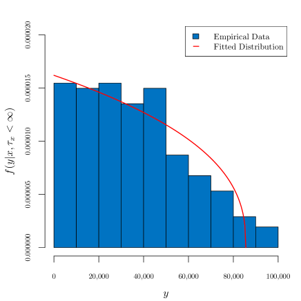
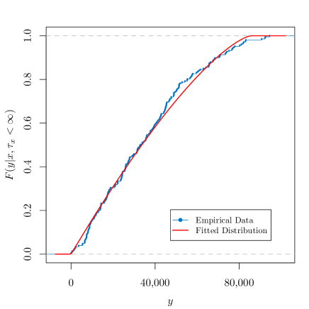
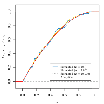
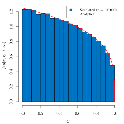
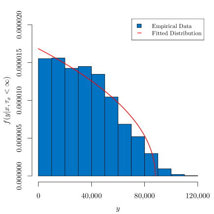
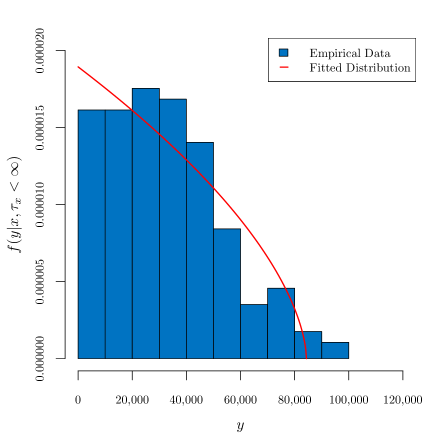
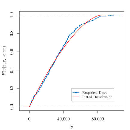
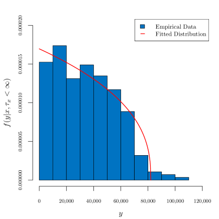
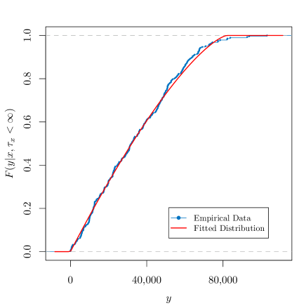
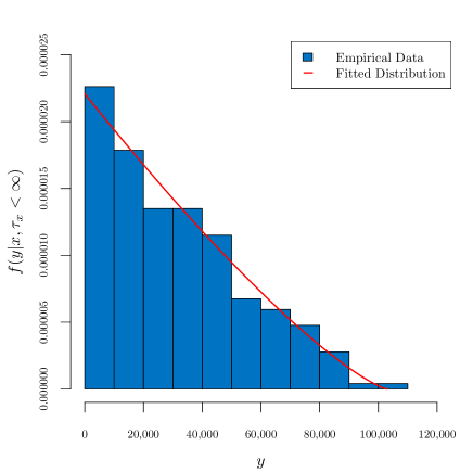
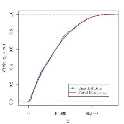
Figure 3 compares both, analytical and simulated, distribution and pdf of the capital deficit at trapping given that trapping occurs. Simulated quantities were generated using the Euler-Maruyama method, a well-known technique mainly used to approximate numerical solutions of Stochastic Differential Equations (SDEs) (see, for example, (Kloeden and Eckhard, 1995)). Not surprisingly, Figure 3(a) clearly shows that the simulated quantities converge to the theoretical distribution (4.45) as the number of simulations $n$ increases, while Figure 3(b) displays how the theoretical pdf given by (4.46) perfectly fits the simulated observations.

(a)

(b)

Figure 3: (a) $F(y|x,\tau_{x}<\infty)$ when $Z_{i}\sim Beta(1.75,1)$, $r=1.08$, $\lambda=1$, $x=1.25$, $x^{*}=1$ (b) $f(y|x,\tau_{x}<\infty)$ when $Z_{i}\sim Beta(1.25,1)$, $r=1.08$, $\lambda=1$, $x=1.25$, $x^{*}=1$.

By comparing (3.2) with (4.46) one concludes that the capital deficit at trapping given that trapping occurs follows the beta distribution of the first kind (B1). Indeed, if we denote the random variable $Y:=\mid X_{\tau_{x}}-x^{*}\mid\Big{|}\ \tau_{x}<\infty$, we have that $Y\sim B1(y;b=x^{*},p=1,q=\alpha)$. Similarly, one can write $Y\stackrel{{\scriptstyle d}}{{=}}x^{*}\cdot(1-Z_{i})$, where $\stackrel{{\scriptstyle d}}{{=}}$ denotes equality in distribution.

5 A Class of Poverty Measures and its Connection with the Capital Deficit at Trapping

Poverty measures serve as the main tool for the evaluation of anti-poverty policies (e.g. cash transfer programmes) and poverty itself. Since Sen (1976), following his axiomatic approach, researchers have formulated numerous poverty measures over the years. The Foster-Greer-Thorbecke (FGT) index (Foster et al., 1984) is undoubtedly one of the most important of these poverty measures and has been widely applied in empirical works. In fact, the FGT index has become the standard measure for international poverty assessments and is regularly reported on by individual countries and international organisations such as the World Bank (for a detailed review of the contributions of the FGT index over the 25 years since its publication, see Foster et al. (2010)). The FGT index emerged as an alternative to the “rank weighting” approach, which was originally applied in the “Sen measure” (see Theorem 1 from Sen (1976)), and accounts for the normalised gap and the rank order of a person in the group of the poor. The FGT index contemplates instead a “short-fall weighting” method, which considers the income short-fall expressed as a share of the poverty line.

Let $F(x)$ be the distribution function of the income variable $X$ from a population with continuous pdf $f(x)$ at a given point $x$. The FGT class of poverty measures indexed by $\gamma\geq 0$ is defined as follows

$$FGT_{\gamma}=\int^{z}_{0}\left(\frac{z-x}{z}\right)^{\gamma}f(x)dx,$$ (5.1)

where $z$ is the poverty line. Particular cases of the FGT class of poverty measures include $FGT_{0}$, which is simply the head-count index and as mentioned in Section 1, calculates the proportion of households living below the poverty line. Another common measure is $FGT_{1}$, a normalisation of the income-gap ratio originally introduced by Sen (1976). This poverty measure is commonly referred to as the poverty gap index. In contrast, the poverty severity index, $FGT_{2}$, is a weighted sum of income short-falls (as a proportion of the poverty line), where the weights are the proportionate income short-falls themselves. Note that, a larger $\gamma$ in (5.1) gives greater emphasis to the poorest poor. Hence, this parameter is viewed as a measure of poverty aversion (Foster et al., 1984).

From (5.1), one can write

$$FGT_{\gamma}=\frac{1}{z^{\gamma}}\mathbbm{E}_{x}\left[D(z,x);x<z\right],$$ (5.2)

with $D(z,x)=\left(z-x\right)^{\gamma}$ a function that describes the level of deprivation suffered by an individual whose income $x$ is less than the poverty line $z$. Clearly, $D(z,x)$ is in terms of an individual’s income short-fall $y:=z-x$.

We now consider a household’s capital process as defined in Section 1. Under this model, a household’s income is generated through capital: $I_{t}=bX_{t}$, where $b>0$ holds (see equation (4) in Kovacevic and Pflug (2011)). Taking $b=1$ leads to the case for which a household’s income is equal to its capital. Thus, the results obtained in Section 4 also apply to a household’s income. On this basis, from Section 4.2 yields that $Y\sim B1(y;b=x^{*},p=1,q=\alpha)$, where the random variable $Y$ denotes the income short-fall (or income deficit) at trapping given that trapping occurs. In this case, the $FGT_{\gamma}$ index is given in terms of the $\gamma$th moment of $Y$,

$$FGT_{\gamma}=\frac{1}{z^{\gamma}}\mathbbm{E}\left[Y^{\gamma}\right]=\left(\frac{x^{*}}{z}\right)^{\gamma}\frac{B\left(1+\alpha,\gamma\right)}{B\left(1,\gamma\right)},$$ (5.3)

where we used the fact that the $h$th moment of a random variable $W\sim B1(w;b,p,q)$ is given by

$$\mathbbm{E}\left[W^{h}\right]=\frac{b^{h}B(p+q,h)}{B(p,h)},$$ (5.4)

(see, for instance, Table 1 from McDonald (1984)).

Remark 5.1.

One can also compute the $h$th moment of the capital deficit at trapping given that trapping occurs by means of the Gerber-Shiu expected discounted penalty function. Indeed, choosing $w(x_{1},x_{2})=x_{2}^{h}$ yields a modified version of the IDE (4.3), with $A(x)=\alpha\cdot{x^{*}}^{h}\cdot B(\alpha,h+1)\cdot y\left(x\right)^{-\alpha}$ for $y(x)=\frac{x}{x^{*}}$. Thus, solving (4.3) as in Proposition 4.1 yields to the $h$th moment of the discounted capital deficit at trapping,

$$\mathbbm{E}\left[\mid X_{\tau_{x}}-x^{*}\mid^{h}e^{-\delta\tau_{x}};\tau_{x}<\infty\right]=\alpha\cdot{x^{*}}^{h}\cdot B\left(\alpha,h+1\right)\cdot m_{\delta}(x).$$ (5.5)

Setting $\delta=0$ yields $\mathbbm{E}\left[\mid X_{\tau_{x}}-x^{*}\mid^{h};\tau_{x}<\infty\right]$, the $h$th moment of the capital deficit at trapping. Consequently, the $h$th moment of the capital deficit at trapping given that trapping occurs is given by

$$\mathbbm{E}\left[Y^{h}\right]:=\frac{\mathbbm{E}\left[\mid X_{\tau_{x}}-x^{*}\mid^{h};\tau_{x}<\infty\right]}{\psi(x)}=\alpha\cdot{x^{*}}^{h}\cdot B\left(\alpha,h+1\right)=\frac{\alpha\cdot x^{*h}\cdot h\cdot B(\alpha,h)}{h+\alpha},$$ (5.6)

where we applied the property $B(p,q+1)=\frac{q\cdot B(p,q)}{p+q}$ of the beta function. Clearly, (5.6) is equal to (5.4) for the case $b=x^{*}$, $p=1$ and $q=\alpha$.

6 An Application to Burkina Faso’s Household Microdata

6.1 Context and Data

Burkina Faso is located in West Africa with an area of $274,200$ $\text{km}^{2}$. In 2021, the population was estimated at just over $20.3$ million, with the capital Ouagadougou being the country’s largest city. Historically, its economy has been largely based on agriculture, which provides a living for more than $80\%$ of the population. Burkina Faso’s main subsistence crops are sorghum, millet, maize and rice, while the country has been one of Africa’s leading producers of cotton and gold (Brugger and Zanetti, 2020; Engels, 2023).

The country’s climate is characterised by a dry tropical climate that alternates a short rainy season with a long dry season. Due to its geographical location, bordering the Sahara Desert, Burkina Faso’s climate is subject to seasonal and annual variations. Furthermore, the country is divided into three different climatic zones, the Sahelian zone in the north, the North-Sudanian zone in the centre and the South-Sudanian zone in the south, which receive an average annual rainfall of less than $600$ mm, between $600$ and $900$ mm and more than $900$ mm, respectively (Alvar-Beltrán et al., 2020).

Household microdata from Burkina Faso’s Continuous Multisector Survey (Enquête Multisectorielle Continue (EMC)) 2014 is used to evaluate the adequacy of the $B1(y;b=x^{*},p=1,q=\alpha)$ model to describe income short-fall distribution. The survey was conducted from 17 January 2014 to 24 November 2014 by the National Institute of Statistics and Demography (Institut National de la Statistique et de la Démographie (INSD)). The EMC had as main objective the generation of sound data for poverty analyses. A total of $10,411$ households were interviewed, with a $96.4\%$ of interviews accepted.

The main variable of interest generated in the survey is consumption, which in the EMC is given in units of the West African CFA (Communauté financière en Afrique) franc per person per day in average prices in Ouagadougou during the EMC field work. To identify the poor, a minimum food basket of around thirty products was defined. Determining the cost of this food basket and other basic needs, the absolute poverty line was estimated at $153,530$ CFA. A person is poor if he/she lives in a poor household and a household is poor if the annual per capita consumption is below the absolute poverty line which is equivalent to $421$ CFA per capita consumption per day.

6.2 Estimators for Parameters of the B1 Model

In this article, we use the method-of-moments (MoM) to estimate the parameters $\alpha$ and $x^{*}$ of the B1 model. Assume that $y_{1},y_{2},...,y_{n}$ is a random sample of income short-fall of size $n$. Letting $M_{k}=\frac{1}{n}\sum\limits^{n}_{i=1}y^{k}_{i}$ denote the $k$th sample moment yields to the method-of-moments estimators (MMEs) for $\alpha$ and $x^{*}$, given by

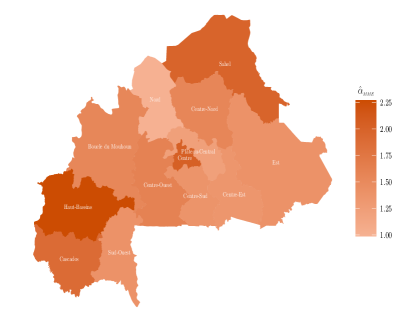
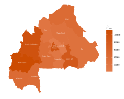
respectively. These estimators are derived by equating the first two sample moments ($M_{1}$ and $M_{2}$) with the theoretical moments (equation (5.6) for $h=1,2$) and by subsequently solving for the two parameters, $\alpha$ and $x^{*}$. Tables 1, 2 and 3 show the MMEs for $\alpha$ and $x^{*}$ at a national level, by area of residence and by region, respectively. In addition, the maps in Figure 4 display these estimates by region, giving a comprehensive geographical overview of the parameters. These results will be discussed more in detail in Section 6.4.

6.3 Evaluating the Goodness-of-Fit of the B1 Model

The non-parametric one-sample Kolmogorov-Smirnov (KS) test and the $R^{2}$ coefficient are used to assess the goodness-of-fit of the B1 model. To conduct the KS test, we calculate the KS statistic, which is given by

$$D=\max_{y}\left|F_{n}(y)-F(y)\right|,$$ (6.1)

where $F_{n}(y)$ is the empirical distribution function defined as $F_{n}(y)=\frac{1}{n}\sum\limits^{n}_{i=1}\mathbbm{1}_{\{y_{i}\leq y\}}$ and $F(y)$ is (4.45), the distribution function of the B1 model. The null ($H_{0}$) and alternative ($H_{1}$) hypotheses of the KS goodness-of-fit test are:

$H_{0}$: the household income short-fall data follows the B1 model and

$H_{1}$: the household income short-fall data does not follows the B1 model.

The null hypothesis $H_{0}$ is rejected at a significance level $\alpha_{{\scaleto{KS}{3pt}}}$ if the p-value of the KS statistic is less than $\alpha_{{\scaleto{KS}{3pt}}}$. The p-value is computed based on the limiting distribution of the KS statistic (6.1) (Marsaglia et al., 2003),

$$\lim_{n\rightarrow\infty}\mathbbm{P}(\sqrt{n}D\leq y)=\frac{\sqrt{2\pi}}{y}\sum_{i=1}^{\infty}e^{-(2i-1)^{2}\pi^{2}/\left(8y^{2}\right)}.$$ (6.2)

We further support the KS test by considering the $R^{2}$ coefficient, which quantifies the degree of correlation between the observed and predicted probabilities under an assumed distribution. Here, a value of $R^{2}$ that is close to one indicates that the B1 model is a good fit for the household income short-fall data. The $R^{2}$ coefficient is computed as follows:

$$R^{2}=\frac{\sum\limits_{i=1}^{n}\left[\hat{F}\left(y_{i}\right)-\bar{F}(y)\right]^{2}}{\sum\limits_{i=1}^{n}\left[\hat{F}\left(y_{i}\right)-\bar{F}(y)\right]^{2}+\sum\limits_{i=1}^{n}\left[F_{n}\left(y_{i}\right)-\hat{F}\left(y_{i}\right)\right]^{2}},$$ (6.3)

where $F_{n}(y_{i})$ is the empirical distribution function for the $i$th household income short-fall, $\hat{F}(y_{i})$ is the estimated distribution function for the $i$th household income short-fall under the B1 model and $\bar{F}(y)$ is the average of $\hat{F}(y_{i})$.

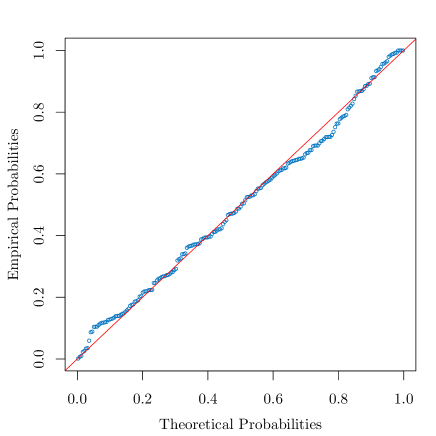
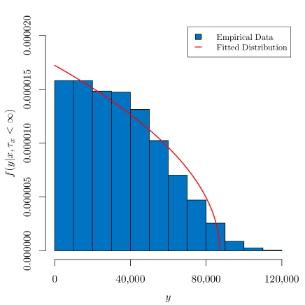
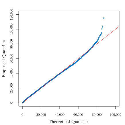
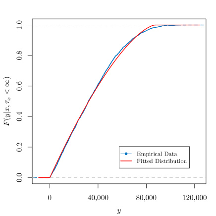
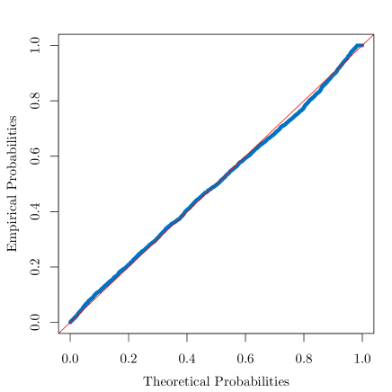
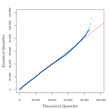
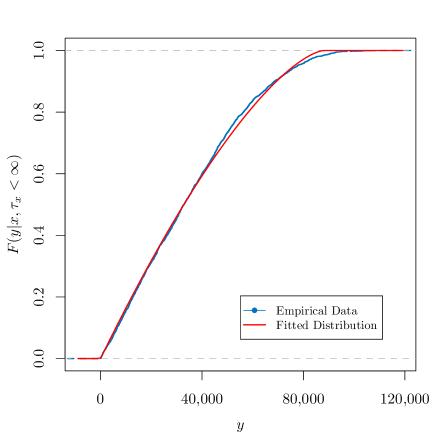
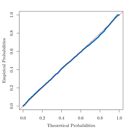
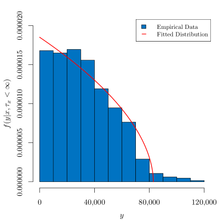
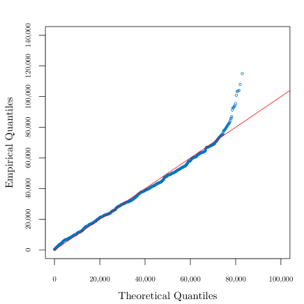
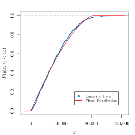
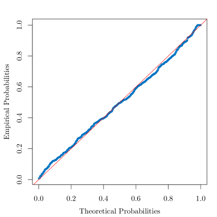
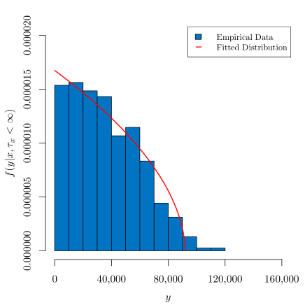
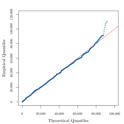
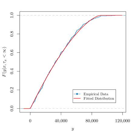
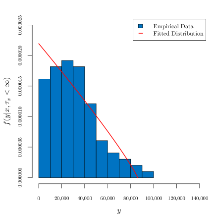
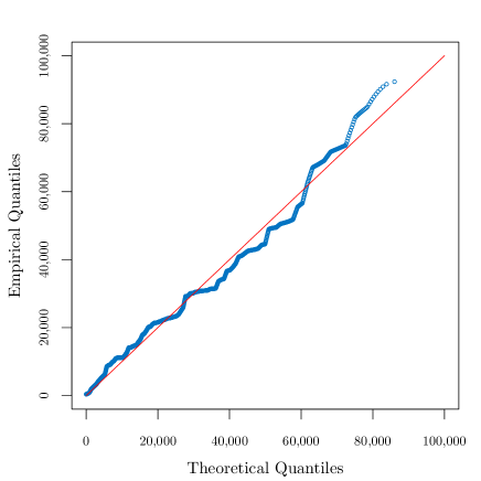
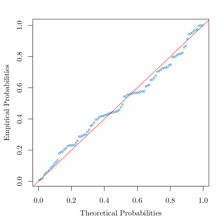
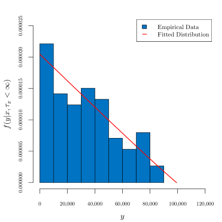
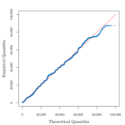
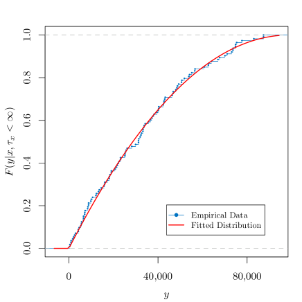
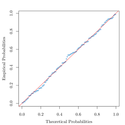
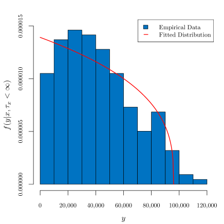
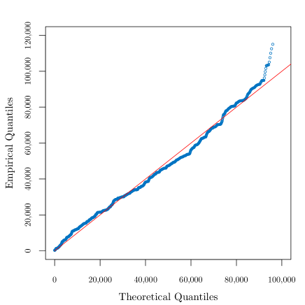
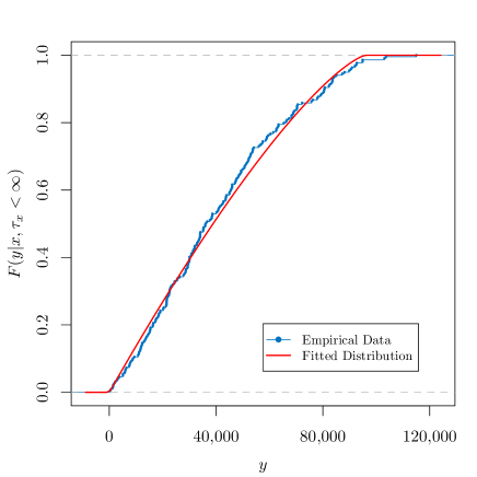
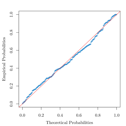
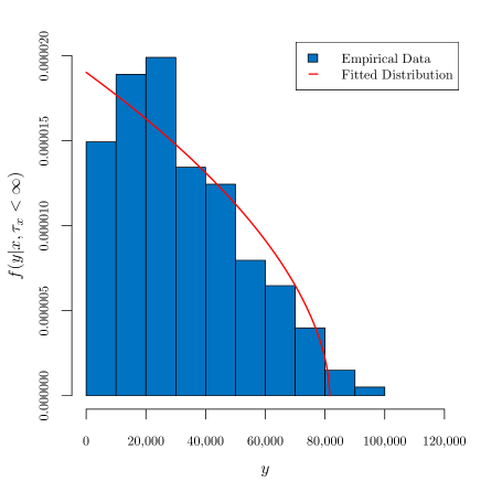
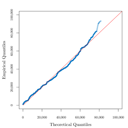
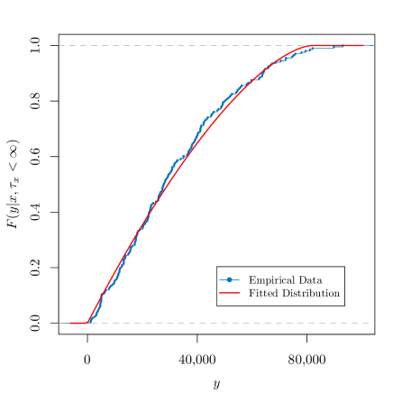
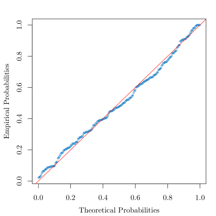
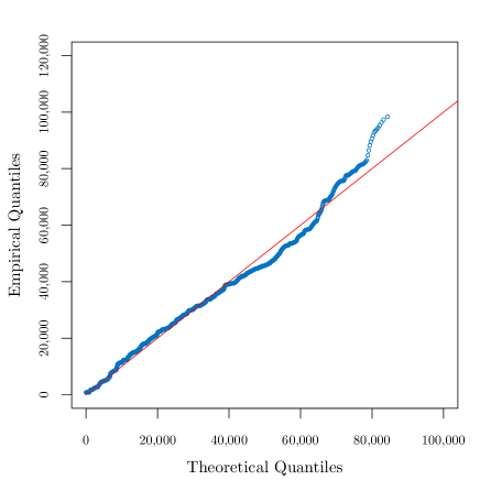
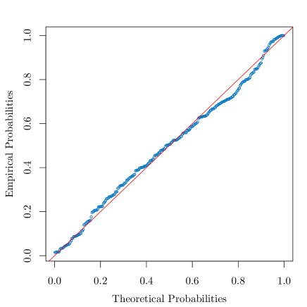
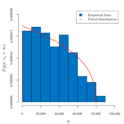
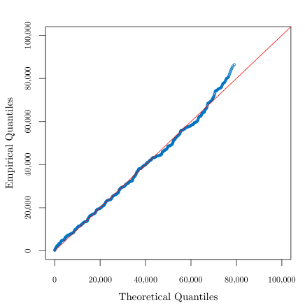
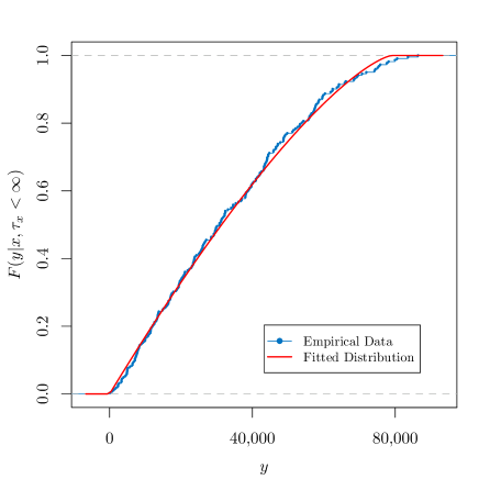
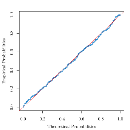
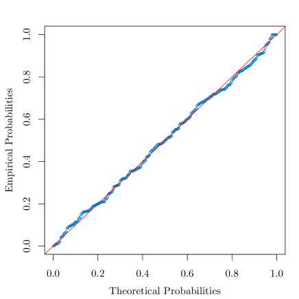
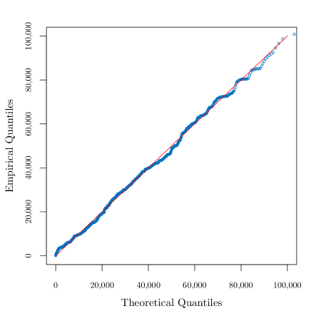
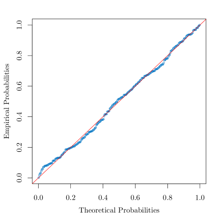
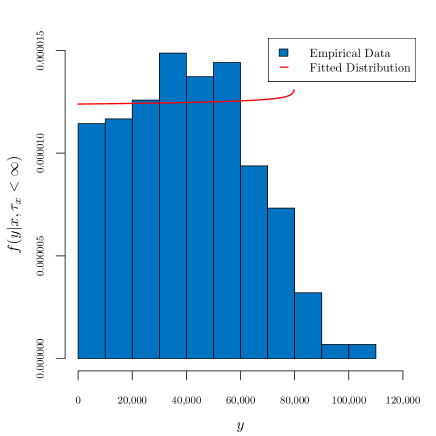
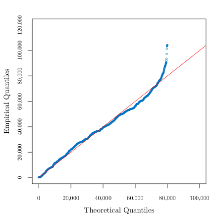
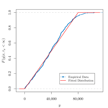
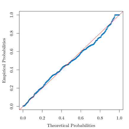
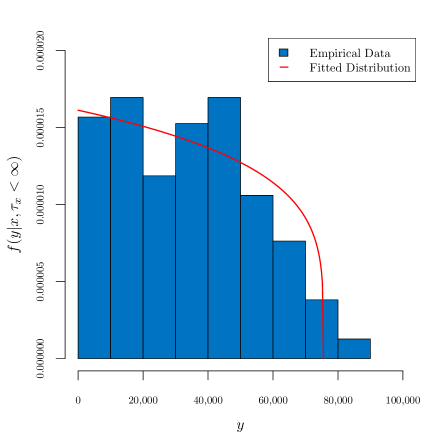
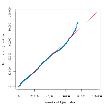
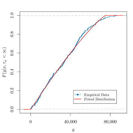
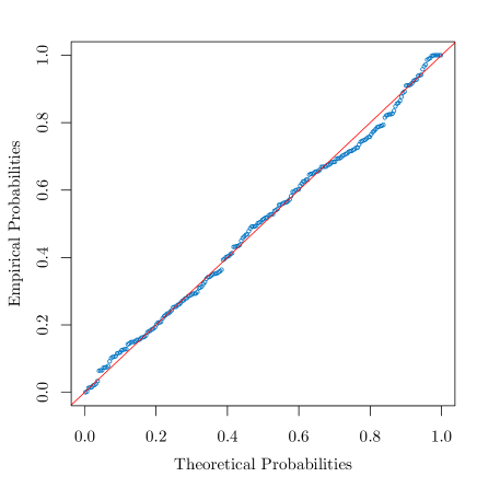
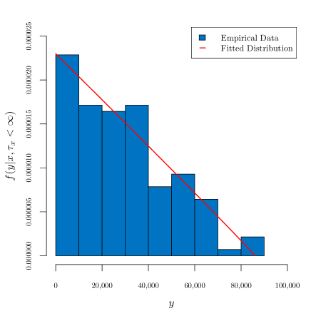
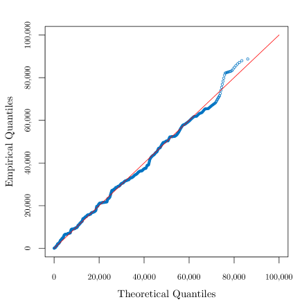
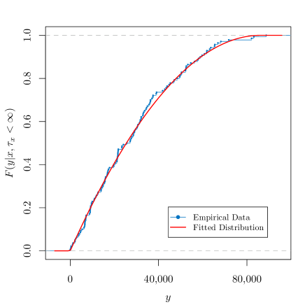
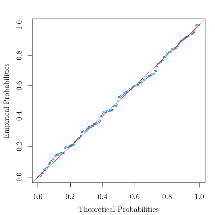
To verify our assumptions and model specifications, we also consider graphical methods. We plot the distribution function (4.45) and the pdf (4.46) against the empirical distribution $F_{n}(y)$ and the histogram of the observed income short-fall data, respectively. In addition, we use the B1 model quantile-quantile (Q-Q) and probability-probability (P-P) plots to support the assumption of a $B1(y;b=x^{*},p=1,q=\alpha)$ distribution. Appendices A, B and C show these graphical methods at a national level, by area of residence and by region, respectively.

6.4 Results and Discussion

The assumption of the B1 distribution can be investigated based on the p-value of the Kolmogorov-Smirnov (KS) statistic and the $R^{2}$ coefficient, which are shown in Tables 1, 2 and 3. As shown in these Tables, with the exception of the estimates at a national level, all p-values of the KS test are higher than the significance level of $\alpha_{{\scaleto{KS}{3pt}}}=0.05$. This indicates that the B1 model significantly describes the household income short-fall data by both area of residence and by region. This is borne out by the estimated values for the $R^{2}$ coefficient, which are found higher than $0.99$ for almost all the cases, suggesting that the B1 model explains more than $99\%$ of the variation in the data, but the remaining (less than $1\%$) variation is attributed to errors and cannot be explained by the model. The Cascades region is the only case attaining a lower value for the $R^{2}$ coefficient: $0.9870$, which is nevertheless still very close to one, so that the model can still be considered to describe a large part of the variation in the data.

Country	Type	$\mathrm{\alpha}$	$x^{*}$	p-value (KS test)	$R^{2}$	Poverty Gap Index ($FGT_{1}$)	Poverty Severity Index ($FGT_{2}$)
Burkina Faso	Direct	-	-	-	-	0.096	0.032
Burkina Faso	MME	1.50	87,209.01	0.02379	0.9983	0.091	0.029
*p-value$>\alpha_{{\scaleto{KS}{3pt}}}=0.05.$

Table 1: B1 distribution fitted parameters and poverty measures for Burkina Faso.

Area of Residence	Type	$\mathrm{\alpha}$	$x^{*}$	p-value (KS test)	$R^{2}$	Poverty Gap Index ($FGT_{1}$)	Poverty Severity Index ($FGT_{2}$)
Urban	Direct	-	-	-	-	0.052	0.016
Urban	MME	1.53	82,925.53	0.4103	0.9961	0.051	0.016
Rural	Direct	-	-	-	-	0.118	0.040
Rural	MME	1.48	88,002.48	0.0754	0.9985	0.111	0.036
*p-value$>\alpha_{{\scaleto{KS}{3pt}}}=0.05.$

Table 2: B1 distribution fitted parameters and poverty measures by area of residence.

Region	Type	$\mathrm{\alpha}$	$x^{*}$	p-value (KS test)	$R^{2}$	Poverty Gap Index ($FGT_{1}$)	Poverty Severity Index ($FGT_{2}$)
Boucle du Mouhoun	Direct	-	-	-	-	0.143	0.052
Boucle du Mouhoun	MME	1.54	91,848.66	0.8662	0.9986	0.131	0.044
Cascades	Direct	-	-	-	-	0.038	0.011
Cascades	MME	1.89	86,053.24	0.7089	0.9870	0.038	0.011
Centre	Direct	-	-	-	-	0.037	0.012
Centre	MME	2.03	99,257.41	0.9487	0.9974	0.037	0.012
Centre-Est	Direct	-	-	-	-	0.096	0.036
Centre-Est	MME	1.34	95,997.68	0.493	0.9931	0.092	0.035
Centre-Nord	Direct	-	-	-	-	0.082	0.026
Centre-Nord	MME	1.55	81,599.65	0.8051	0.9937	0.075	0.023
Centre-Ouest	Direct	-	-	-	-	0.107	0.034
Centre-Ouest	MME	1.60	84,363.89	0.3283	0.9930	0.099	0.030
Centre-Sud	Direct	-	-	-	-	0.095	0.030
Centre-Sud	MME	1.37	79,048.83	0.9878	0.9978	0.090	0.027
Est	Direct	-	-	-	-	0.109	0.035
Est	MME	1.39	82,056.03	0.9768	0.9980	0.104	0.033
Hauts-Bassins	Direct	-	-	-	-	0.076	0.025
Hauts-Bassins	MME	2.27	102,924.19	0.7671	0.9974	0.072	0.023
Nord	Direct	-	-	-	-	0.176	0.063
Nord	MME	0.99	79,977.12	0.1357	0.9928	0.170	0.059
Plateau Central	Direct	-	-	-	-	0.104	0.034
Plateau Central	MME	1.22	75,536.12	0.7121	0.9963	0.097	0.030
Sahel	Direct	-	-	-	-	0.050	0.015
Sahel	MME	1.98	86,059.27	0.9505	0.9973	0.048	0.013
Sud-Ouest	Direct	-	-	-	-	0.081	0.027
Sud-Ouest	MME	1.39	85,579.68	0.4962	0.9941	0.082	0.027
*p-value$>\alpha_{{\scaleto{KS}{3pt}}}=0.05.$

Table 3: B1 distribution fitted parameters and poverty measures by region.

Graphical methods displayed in Appendices A, B and C provide an additional tool to evaluate the assumption of the B1 distribution. Plot (a) in the Appendices shows a density plot in which are plotted the pdf (4.46) of a B1 model and the histogram of the observed income short-fall data. On the other hand, plot (c) in the Appendices displays a distribution plot in which the B1 distribution function (4.45) is plotted against the empirical distribution function $F_{n}(y)$. From these plots, one can observe that the B1 model fits the histogram and the empirical distribution well, respectively. Moreover, if the household income short-fall data is found to follow the B1 model, observations on both the quantile-quantile (Q-Q) and probability-probability (P-P) plots will appear to form almost a straight diagonal line. In general, household income short-fall data is positioned in the diagonal by area of residence and by region, suggesting the appropriateness of the B1 distribution. In particular, one cannot expect the observed income short-fall data points to follow the reference diagonal line in the upper quantiles as income short-fall data is sparse in the tails.

As underlined in Section 6.2, parameter estimates are based on the Method of Moments (MoM) and are shown in Tables 1, 2 and 3. From Section 1, one can realise that under the assumption of $Beta(\alpha,1)-$distributed remaining proportions of capital, higher values of $\alpha$ yield to a greater expected remaining proportion of capital upon experiencing a capital loss (i.e. the distribution is left-skewed or equivalently, the remaining proportions of capital $Z_{i}\in[0,1]$ are more likely to have values close to one). On this basis, it is possible to assess the magnitude of capital losses experienced by households in Burkina Faso. For instance, Figure 4(a) displays how households experience capital losses of varying magnitude depending on the geographical area in which they reside. In fact, Figure 4(a) shows interestingly that these magnitudes appear to be linked to or dependent on the different climatic zones. These findings are in line with previous research, which highlights the country’s economy dependence on rain-fed agriculture and livestock husbandry, which in turn makes it vulnerable to climate risks such as droughts and floods (see, for example, Zampaligré et al. (2014)). In particular, Table 2 and Figure 4(b) show that the estimates of the critical capital $x^{*}$ for Hauts-Bassins, Centre-Est, Centre and Boucle du Mouhoun are higher (greater than 90,000 CFA), compared to those for the rest of regions, suggesting that the country’s potentially poorest households live in these regions. However, it is important to note that the poverty gap index ($FGT_{1}$) and the poverty severity index ($FGT_{2}$) shown in Table 2 for Boucle du Mouhoun attain higher values due to the fact that the head-count index is higher (56%) compared to that of Hauts-Bassins (35%), Centre-Est (34%) and Centre (17%). Similarly, households residing in the Nord region seem to experience the most adverse capital losses, as its estimated value for $\alpha$ shown in Table 2 is the lowest among all regions. Moreover, Nord’s high head-count index (65%) and its uniform distribution shape are major contributors to the high poverty gap ($FGT_{1}$) and poverty severity ($FGT_{2}$) index.

(a)

(b)

Figure 4: Method of moment estimators (MMEs) by region: (a) $\hat{\alpha}_{{\scaleto{MME}{3pt}}}$ (b) $\hat{x^{*}}_{{\scaleto{MME}{3pt}}}$.

The robustness of the poverty gap index ($FGT_{1}$) and the poverty severity index ($FGT_{2}$) at a national level, by area of residence and by region, when specifying the B1 model as the income short-fall distribution can be evaluated in Tables 1, 2 and 3, respectively. Comparing the estimates using the B1 distribution assumption with the direct (empirical) values of the poverty measures, one can see how close the estimates are to the direct values of the FGT indices, thus reinforcing the assumption of the B1 distribution for income short-fall data.

Figure 5: Sensitivity of the poverty gap and the poverty severity index to $\alpha$ and $x^{*}$ for selected regions. Markers show the actual values of the poverty measures.

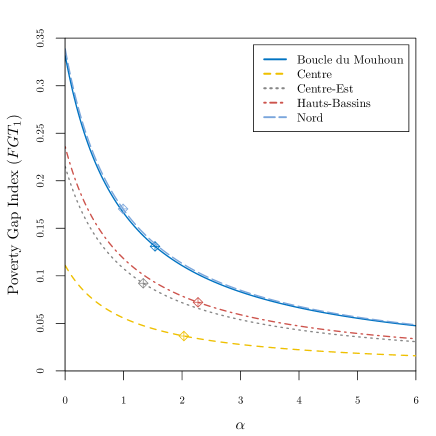
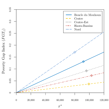
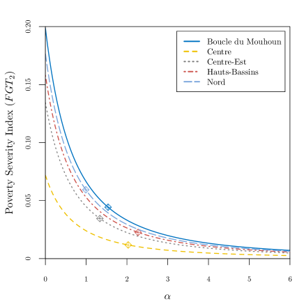
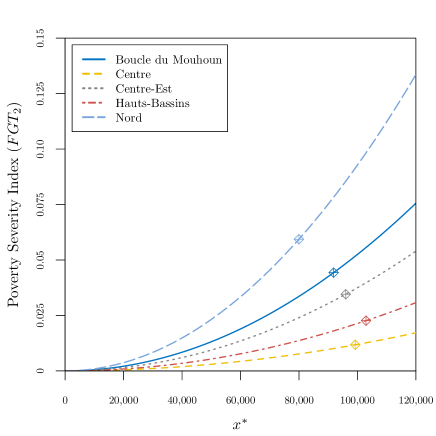
In Figure 5, we contrast the level of poverty and the changes that would have occurred in the poverty level of selected regions. Both the poverty gap and the poverty severity index show an enormous progress in poverty reduction for greater expected remaining proportion of capital upon experiencing a capital loss (i.e. higher values of $\alpha$). Higher values for $\alpha$ can be attained with risk mitigation strategies such as subsidised insurance programmes (Flores-Contró et al., 2021). Similarly, as expected, Figure 5 shows that for higher values of critical capital $x^{*}$, poverty level increases.

7 Conclusion

This article studies the Gerber-Shiu expected discounted penalty function for the household capital process introduced in Kovacevic and Pflug (2011). The Gerber-Shiu function incorporates information on the trapping time, the capital surplus immediately before trapping and the capital deficit at trapping. Recent work focuses on only analysing the infinite-time trapping probability (Henshaw et al., 2023), therefore overlooking quantities of particular interest such as the undershoot and the overshoot of a household’s capital at trapping. To the best of our knowledge, we derive for the first time a functional equation for the Gerber-Shiu function and we solve it for the particular case in which the remaining proportions of capital upon experiencing a capital loss are $Beta(\alpha,1)-$distributed. As a result, we obtain closed-form expressions for important quantities such as the Laplace transform of the trapping time and the distribution of the capital deficit at trapping. These quantities are particularly important as they provide crucial information towards understanding a household’s transition into poverty.

Using risk theory techniques, we derive a microeconomic foundation for the beta of the first kind (B1) as a suitable model to represent the distribution of personal income deficit (or income short-fall). It is indeed interesting that our findings are in line with previous research in development economics, where the generalised beta (GB) distribution family and its derivatives (including the B1 model) have shown to be appropriate models to describe the distribution of personal income.

Affinities between the capital deficit at trapping and a class of poverty measures, known as the Foster-Greer-Thorbecke (FGT) index, are also presented. In addition, we provide empirical evidence of the suitability of the B1 distribution for modelling Burkina Faso’s household income short-fall data from the Continuous Multisector Survey (Enquête Multisectorielle Continue (EMC)) 2014. Indeed, in this article, the B1 model is fitted to Burkina Faso’s household income short-fall data, and it is found that the B1 distribution fitted to the data well, suggesting that this model is appropriate for describing the income short-fall distribution. Moreover, we show how the poverty gap index and the poverty severity index can be calculated from the estimated B1 income short-fall distribution. One of the main advantages of parametric distributions such as the B1 distribution is that (poverty) indicators can be presented as functions of the parameters of the chosen distribution. Thus parametric modeling allows to gain insight into the relationship between (poverty) indicators and the distribution of the parameters.

Future research can consider other distributions supported in $[0,1]$ for the remaining proportions of capital. In this way, one could arrive at other distributions for the capital deficit at trapping that have also been used previously to model personal income (e.g. the lognormal distribution and the power-law distribution). However, this is not straightforward, as finding a closed-form solution for the Integro-Differential Equation (IDE) derived in Theorem 4.1 when considering more general distributions for the remaining proportion of capital is challenging. In addition, it might also be interesting to carry out the same analysis with household microdata from other countries in order to verify the results obtained with Burkina Faso’s EMC.

Appendices

A Goodness-of-Fit Plots for Burkina Faso

Burkina Faso

(a) Comparison of Probability Density

(b) Quantile-Quantile (Q-Q) Plot

(c) Comparison of Probability Distributions

(d) Probability-Probability (P-P) Plot

B Goodness-of-Fit Plots by Area of Residence

Rural

(a) Comparison of Probability Density

(b) Quantile-Quantile (Q-Q) Plot

(c) Comparison of Probability Distributions

(d) Probability-Probability (P-P) Plot

Urban

(a) Comparison of Probability Density

(b) Quantile-Quantile (Q-Q) Plot

(c) Comparison of Probability Distributions

(d) Probability-Probability (P-P) Plot

C Goodness-of-Fit Plots by Region

Boucle du Mouhoun

(a) Comparison of Probability Density

(b) Quantile-Quantile (Q-Q) Plot

(c) Comparison of Probability Distributions

(d) Probability-Probability (P-P) Plot

Cascades

(a) Comparison of Probability Density

(b) Quantile-Quantile (Q-Q) Plot

(c) Comparison of Probability Distributions

(d) Probability-Probability (P-P) Plot

Centre

(a) Comparison of Probability Density

(b) Quantile-Quantile (Q-Q) Plot

(c) Comparison of Probability Distributions

(d) Probability-Probability (P-P) Plot

Centre-Est

(a) Comparison of Probability Density

(b) Quantile-Quantile (Q-Q) Plot

(c) Comparison of Probability Distributions

(d) Probability-Probability (P-P) Plot

Centre-Nord

(a) Comparison of Probability Density

(b) Quantile-Quantile (Q-Q) Plot

(c) Comparison of Probability Distributions

(d) Probability-Probability (P-P) Plot

Centre-Ouest

(a) Comparison of Probability Density

(b) Quantile-Quantile (Q-Q) Plot

(c) Comparison of Probability Distributions

(d) Probability-Probability (P-P) Plot

Centre-Sud

(a) Comparison of Probability Density

(b) Quantile-Quantile (Q-Q) Plot

(c) Comparison of Probability Distributions

(d) Probability-Probability (P-P) Plot

Est

(a) Comparison of Probability Density

(b) Quantile-Quantile (Q-Q) Plot

(c) Comparison of Probability Distributions

(d) Probability-Probability (P-P) Plot

Hauts-Bassins

(a) Comparison of Probability Density

(b) Quantile-Quantile (Q-Q) Plot

(c) Comparison of Probability Distributions

(d) Probability-Probability (P-P) Plot

Nord

(a) Comparison of Probability Density

(b) Quantile-Quantile (Q-Q) Plot

(c) Comparison of Probability Distributions

(d) Probability-Probability (P-P) Plot

Plateau Central

(a) Comparison of Probability Density

(b) Quantile-Quantile (Q-Q) Plot

(c) Comparison of Probability Distributions

(d) Probability-Probability (P-P) Plot

Sahel

(a) Comparison of Probability Density

(b) Quantile-Quantile (Q-Q) Plot

(c) Comparison of Probability Distributions

(d) Probability-Probability (P-P) Plot

Sud-Ouest

(a) Comparison of Probability Density

(b) Quantile-Quantile (Q-Q) Plot

(c) Comparison of Probability Distributions

(d) Probability-Probability (P-P) Plot

References

- Abramowitz and Stegun (1972) Abramowitz, M. and I. A. Stegun (1972). Handbook of Mathematical Functions with Formulas, Graphs, and Mathematical Tables. Washington, D.C.: U.S. Department of Commerce.
- Altman et al. (2002) Altman, E., K. E. Avrachenkov, C. Barakat, and R. Núñez-Queija (2002). State-Dependent M/G/1 Type Queueing Analysis for Congestion Control in Data Networks. Computer Networks 39(6), 789–808.
- Altman et al. (2005) Altman, E., K. E. Avrachenkov, A. A. Kherani, and B. J. Prabhu (2005). Performance Analysis and Stochastic Stability of Congestion Control Protocols. In Proceedings IEEE 24th Annual Joint Conference of the IEEE Computer and Communications Societies., Volume 2, pp. 1316–1327. IEEE.
- Alvar-Beltrán et al. (2020) Alvar-Beltrán, J., A. Dao, A. Dalla Marta, A. Heureux, J. Sanou, and S. Orlandini (2020). Farmers’ Perceptions of Climate Change and Agricultural Adaptation in Burkina Faso. Atmosphere 11(8).
- Ancarani and Gasaneo (2009) Ancarani, L. U. and G. Gasaneo (2009). Derivatives of Any Order of the Gaussian Hypergeometric Function with Respect to the Parameters , and . Journal of Physics A: Mathematical and Theoretical 42(39), 395208.
- Appell and Kampé De Fériet (1926) Appell, P. and J. Kampé De Fériet (1926). Fonctions Hypergéométriques et Hypersphériques: Polynomes d’Hermite. Paris: Gauthier-Villars.
- Asmussen and Albrecher (2010) Asmussen, S. and H. Albrecher (2010). Ruin Probabilities. Singapore: World Scientific.
- Azaïs and Genadot (2015) Azaïs, R. and A. Genadot (2015). Semi-Parametric Inference for the Absorption Features of a Growth-Fragmentation Model. TEST 24(2), 341–360.
- Booth (1889) Booth, C. (1889). Labour and Life of the People. London: Williams and Norgate.
- Brugger and Zanetti (2020) Brugger, F. and J. Zanetti (2020). “In My Village, Everyone Uses the Tractor”: Gold Mining, Agriculture and Social Transformation in Rural Burkina Faso. The Extractive Industries and Society 7(3), 940–953.
- Callealta Barroso et al. (2020) Callealta Barroso, F. J., C. García-Pérez, and M. Prieto-Alaiz (2020). Modelling Income Distribution Using the Student’s Distribution: New Evidence for European Union Countries. Economic Modelling 89, 512–522.
- Chiu and Yin (2003) Chiu, S. N. and C. C. Yin (2003). The Time of Ruin, the Surplus Prior to Ruin and the Deficit at Ruin for the Classical Risk Process Perturbed by Diffusion. Insurance: Mathematics and Economics 33(1), 59–66.
- Cramér (1930) Cramér, H. (1930). On the Mathematical Theory of Risk. Stockholm: Centraltryckeriet.
- Davis (1984) Davis, M. H. A. (1984). Piecewise-Deterministic Markov Processes: A General Class of Non-Diffusion Stochastic Models. Journal of the Royal Statistical Society: Series B (Methodological) 46(3), 353–388.
- Davis (1993) Davis, M. H. A. (1993). Markov Models & Optimization, Volume 49 of Monographs on Statistics and Applied Probability. New Delhi: Chapman & Hall.
- Derfel et al. (2012) Derfel, G., B. van Brunt, and G. C. Wake (2012). A Cell Growth Model Revisited. Functional Differential Equations 19(1–2), 71–81.
- Eliazar and Klafter (2004) Eliazar, I. and J. Klafter (2004). A Growth–Collapse Model: Lévy Inflow, Geometric Crashes, and Generalized Ornstein–Uhlenbeck Dynamics. Physica A: Statistical Mechanics and its Applications 334(1), 1–21.
- Eliazar and Klafter (2006) Eliazar, I. and J. Klafter (2006). Growth-Collapse and Decay-Surge Evolutions, and Geometric Langevin Equations. Physica A: Statistical Mechanics and its Applications 367, 106–128.
- Engels (2023) Engels, B. (2023). Disparate But Not Antagonistic: Classes of Labour in Cotton Production in Burkina Faso. Journal of Agrarian Change 23(1), 149–166.
- Flores-Contró et al. (2021) Flores-Contró, J. M., K. Henshaw, S. H. Loke, S. Arnold, and C. D. Constantinescu (2021). Subsidising Inclusive Insurance to Reduce Poverty. Working Paper.
- Foster et al. (1984) Foster, J., J. Greer, and E. Thorbecke (1984). A Class of Decomposable Poverty Measures. Econometrica: Journal of the Econometric Society 52(3), 761–766.
- Foster et al. (2010) Foster, J., J. Greer, and E. Thorbecke (2010). The Foster–Greer–Thorbecke (FGT) Poverty Measures: 25 Years Later. The Journal of Economic Inequality 8(4), 491–524.
- Gauss (1866) Gauss, C. F. (1866). Disquisitiones Generales Circa Seriem Infinitam. Ges. Werke Gottingen 2, 437–45.
- Gerber and Shiu (1997) Gerber, H. U. and E. S. Shiu (1997). The Joint Distribution of the Time of Ruin, the Surplus Immediately Before Ruin, and the Deficit at Ruin. Insurance: Mathematics and Economics 21(2), 129–137.
- Gerber and Shiu (1998) Gerber, H. U. and E. S. Shiu (1998). On the Time Value of Ruin. North American Actuarial Journal 2(1), 48–72.
- Graf and Nedyalkova (2014) Graf, M. and D. Nedyalkova (2014). Modeling of Income and Indicators of Poverty and Social Exclusion Using the Generalized Beta Distribution of the Second Kind. Review of Income and Wealth 60(4), 821–842.
- Harrison (1977) Harrison, J. M. (1977). Ruin Problems with Compounding Assets. Stochastic Processes and their Applications 5(1), 67–79.
- He et al. (2023) He, Y., R. Kawai, Y. Shimizu, and K. Yamazaki (2023). The Gerber-Shiu Discounted Penalty Function: A Review from Practical Perspectives. Insurance: Mathematics and Economics 109, 1–28.
- Henshaw et al. (2023) Henshaw, K., J. M. Ramirez, J. M. Flores-Contró, E. A. Thomann, S. H. Loke, and C. D. Constantinescu (2023). On the Impact of Insurance on Households Susceptible to Random Proportional Losses: An Analysis of Poverty Trapping. Working Paper.
- Hlasny (2021) Hlasny, V. (2021). Parametric Representation of the Top of Income Distributions: Options, Historical Evidence, and Model Selection. Journal of Economic Surveys 35(4), 1217–1256.
- Institut National de la Statistique et de la Démographie (INSD) (2015) Institut National de la Statistique et de la Démographie (INSD) (2015). Rapport Enquête Multisectorielle Continue (EMC) 2014. Ministère de l’Économie et des Finances du Burkina Faso.
- Kloeden and Eckhard (1995) Kloeden, P. E. and P. Eckhard (1995). Numerical Solution of Stochastic Differential Equations. United States of America: Springer-Verlag.
- Kovacevic and Pflug (2011) Kovacevic, R. M. and G. C. Pflug (2011). Does Insurance Help to Escape the Poverty Trap? — A Ruin Theoretic Approach. Journal of Risk and Insurance 78(4), 1003–1027.
- Kovacevic and Semmler (2021) Kovacevic, R. M. and W. Semmler (2021). Poverty Traps and Disaster Insurance in a Bi-level Decision Framework. In J. L. Haunschmied, R. M. Kovacevic, W. Semmler, and V. M. Veliov (Eds.), Dynamic Economic Problems with Regime Switches, Volume 25 of Dynamic Modeling and Econometrics in Economics and Finance, Chapter 3, pp. 57–83. Switzerland: Springer Nature.
- Kyprianou (2013) Kyprianou, A. E. (2013). Gerber–Shiu Risk Theory. Switzerland: Springer International Publishing.
- Landriault and Willmot (2009) Landriault, D. and G. E. Willmot (2009). On the Joint Distributions of the Time to Ruin, the Surplus Prior to Ruin, and the Deficit at Ruin in the Classical Risk Model. North American Actuarial Journal 13(2), 252–270.
- Lin and Willmot (1999) Lin, X. S. and G. E. Willmot (1999). Analysis of a Defective Renewal Equation Arising in Ruin Theory. Insurance: Mathematics and Economics 25(1), 63–84.
- Lin and Willmot (2000) Lin, X. S. and G. E. Willmot (2000). The Moments of the Time of Ruin, the Surplus Before Ruin, and the Deficit at Ruin. Insurance: Mathematics and Economics 27(1), 19–44.
- Lundberg (1903) Lundberg, F. (1903). I. Approximerad Framställning af Sannolikhetsfunktionen II. Återförsäkring af Kollektivrisker. Akademisk Afhandling. Uppsala: Almqvist & Wiksell.
- Lundberg (1926) Lundberg, F. (1926). Försäkringsteknisk riskutjämning. Stockholm: F. Englunds boktryckeri A.B.
- Löpker and Van Leeuwaarden (2008) Löpker, A. H. and J. S. H. Van Leeuwaarden (2008). Transient Moments of the TCP Window Size Process. Journal of Applied Probability 45(1), 163–175.
- Marsaglia et al. (2003) Marsaglia, G., W. W. Tsang, and J. Wang (2003). Evaluating Kolmogorov’s Distribution. Journal of Statistical Software 8(18), 1–4.
- McDonald (1984) McDonald, J. B. (1984). Some Generalized Functions for the Size Distribution of Income. Econometrica 52(3), 647–663.
- McDonald and Xu (1995) McDonald, J. B. and Y. J. Xu (1995). A Generalization of the Beta Distribution with Applications. Journal of Econometrics 66(1), 133–152.
- Pareto (1967) Pareto, V. (1967). In G. Busino (Ed.), Ecrits sur la Courbe de la Répartition de la Richesse, Volume 36 of Travaux de Droit, d’Économie, de Sociologie et des Sciences Politiques. Genève: Librairie Droz.
- Paulsen (1998) Paulsen, J. (1998). Ruin Theory with Compounding Assets — A Survey. Insurance: Mathematics and Economics 22(1), 3–16.
- Rowntree (1901) Rowntree, B. S. (1901). Poverty: A Study of Town Life. London: Macmillan.
- Salem and Mount (1974) Salem, A. B. Z. and T. D. Mount (1974). A Convenient Descriptive Model of Income Distribution: The Gamma Density. Econometrica 42(6), 1115–1127.
- Seaborn (1991) Seaborn, J. B. (1991). Hypergeometric Functions and Their Applications. New York: Springer-Verlag.
- Segerdahl (1942) Segerdahl, C. O. (1942). Über einige risikotheoretische fragestellungen. Scandinavian Actuarial Journal (1-2), 43–83.
- Sen (1976) Sen, A. (1976). Poverty: An Ordinal Approach to Measurement. Econometrica 44(2), 219–231.
- Singh and Maddala (1976) Singh, S. K. and G. S. Maddala (1976). A Function for Size Distribution of Incomes. Econometrica 44(5), 963–970.
- Slater (1960) Slater, L. J. (1960). Confluent Hypergeometric Functions. New York: Cambridge University Press.
- Sundt and Teugels (1995) Sundt, B. and J. L. Teugels (1995). Ruin Estimates Under Interest Force. Insurance: Mathematics and Economics 16(1), 7–22.
- Thurow (1970) Thurow, L. C. (1970). Analyzing the American Income Distribution. The American Economic Review 60(2), 261–269.
- Zampaligré et al. (2014) Zampaligré, N., L. H. Dossa, and E. Schlecht (2014). Climate Change and Variability: Perception and Adaptation Strategies of Pastoralists and Agro-Pastoralists Across Different Zones of Burkina Faso. Regional Environmental Change 14(2), 769–783.