Explaining the Machine Learning Solution of the Ising Model

Abstract

As powerful as machine learning (ML) techniques are in solving problems involving data with large dimensionality, explaining the results from the fitted parameters remains a challenging task of utmost importance, especially in physics applications. Here it is shown how this can be accomplished for the ferromagnetic Ising model, the target of many ML studies in the last years. By using a neural network (NN) without any hidden layers and the symmetry of the Hamiltonian to find the critical temperature for the continuous phase transition of the model, an explanation of its strategy is found. This allows the prediction of the minimal extension of the NN to solve the problem when the symmetry is not known, which is also explainable.

From the second part of the 2010’s, the field of statistical physics has experienced an explosion in research using machine learning (ML) techniques to address problems related to phase transitions, mainly the characterization of phase diagrams for both classical and quantum models [1, 2, 3, 4, 5, 6, 7, 8, 9, 10, 11]. At its heart, ML is statistical inference assisted by computational methods in order to fit parametric functions with a very large number of parameters using also very large datasets. ML models, which include neural networks (NNs), support vector machines, random forests and others, are sophisticated parametric families, and the learning algorithms are designed to fit the parameters according to appropriate cost functions while avoiding overfitting.

Due to its simplicity, fundamental character, wide applicability outside physics and the presence of a continuous phase transition [12], the two-dimensional classical Ising model – in particular its ferromagnetic version – has been one of the main targets of ML applications in the field. It has been demonstrated that it is possible to detect the existence of its two phases (ferro and paramagnetic) using unsupervised learning [1, 13] and to approximate the critical temperature for the transition using both unsupervised [14, 15, 10] and supervised learning [2] using as data only the spin configurations at different temperatures. It was also observed that a model trained for a particular lattice topology can infer with success the critical temperature for other lattices, what is usually known in the ML field as transfer learning [2].

The importance of these results stems from the fact that, although simplified, the described scenario corresponds to the actual discovery and characterization of full phase diagrams purely from microscopic experimental data. There is mounting evidence, although there is no general methodology or proofs, that these results can be extended to general phase transitions [2, 5, 16, 17, 18].

For the particular case of the ferromagnetic Ising model, increasingly sophisticated methods have been used to tackle the problem, from one-hidden-layer NNs (1HLNNs) [2, 19] to deep learning architectures [20], such as convolutional neural networks (CNNs) [14] and autoencoders (plain and variational) [13, 10]. Although powerful, a drawback of sophisticated state-of-the-art ML models is that the large number of parameters, allied to the varied choices for hyperparameters (number of layers, units per layer, pooling layers, loss functions and others), make it difficult to extract meaning from the trained models – the more intricate the architecture, the more of a black-box they become. Addressing this point is known as the issue of ‘explainable AI’ (XAI) [21], which became an area of study itself.

Being able to have insights on how a trained ML model solves a problem is fundamental for breaking barriers against their general use, a known problem in health applications where distrust and ethical concerns by professionals who are not ML specialists might lead to decreased adoption, preventing the area from reaping the potential benefits [22]. While the adoption barrier might be lower in areas with less direct human applications, explainability has technical advantages. Unveiling the mechanisms used by a model to infer the necessary patterns might allow improvements in its architecture, which by itself might lead to clearer or more efficient solutions. A yet more fundamental reason for seeking it goes to the heart of physics and scientific research itself. Hidden patterns contained in the structure of the trained models might reveal new physical laws, such as symmetries, leading to new discoveries.

The aim of this letter is to carry out such an analysis. Previous authors [2, 14] have taken important steps towards understanding ML solutions, being able to identify several aspects of the inference. A key study is found in a beautiful work by Kim and Kim [19], who were able to predict and prove that a 1HLNN needs only two hidden units to identify the critical temperature. By analyzing this simplified model, they concluded that the NN used the spin inversion symmetry of the Hamiltonian at zero external field to learn the scaling dimension of the magnetization.

The present work goes one step further to find an even simpler NN (possibly the simplest) that can find the critical temperature of the ferromagnetic Ising model. A full explanation of the solution can then be found, leading to a better understanding for the success of previous models and complementing the work of [19]. The technique used here is at the core of physics research – finding the simplest non-trivial model that is capable of solving the task allows a clearer vision of its inner workings. The solution is found using a NN without any hidden layers, called a single-layer NN (SLNN) for short, trained with data from a single-sized square lattice, without the need for regularization and with data excluding a relatively large asymmetric interval around the known critical temperature. This is accomplished by a physics-informed approach, where (like in [19]) minimal knowledge of the physics of the problem is used to justify the choice of the architecture, in this case the symmetry of the Hamiltonian by full spin inversion. The trained network cannot only find very close estimates for the square lattice, but also for other two-dimensional lattices and, although with less precision, for the cubic one.

To set the notation, let us write the Hamiltonian of the Ising model as

$$H=-\sum_{{\left<i,j\right>}}J_{ij}s_{i}s_{j},$$ (1)

where $s_{i}\in{\left\{-1,1\right\}}$ for $i=1,...,N$, with $N$ the number of spins in the system and $J_{ij}$ the exchange couplings. Local external magnetic fields are considered to be zero in order for the critical phase transition to occur. For each configuration $s=(s_{1},s_{2},...,s_{N})$ of the lattice, the magnetization per spin is given by the average of all the spin values on it $m(s)=\sum_{i}s_{i}/N$, i.e., an equal linear combination of them. Throughout this work, the Boltzmann constant is set to unit, $k_{B}=1$.

Onsager’s solution for an infinite square lattice [23] assumes the couplings $J_{ij}$ are the same in each of the two perpendicular directions in the lattice, $J_{1}$ and $J_{2}$. Here, let us assume for simplicity that $J_{1}=J_{2}=J$. The ferromagnetic transition requires $J>0$, which is the situation considered throughout this letter. The critical temperature is given by $T_{c}=2J/\ln{\left(1+\sqrt{2}\right)}$ and the average magnetization per spin at temperature $T$ is ${\left<m\right>_{T}}=\pm{\left(1-\sinh^{-4}2\beta J\right)}^{1/8}$, $0\leq|{\left<m\right>_{T}}|\leq 1$, where $\beta=1/T$ and the sign is due to the $\mathbb{Z}_{2}$ symmetry of the ferromagnetic phase. For $T<T_{c}$, $|{\left<m\right>_{T}}|\neq 0$ and the system is in the ferromagnetic ordered phase, while for $T>T_{c}$, ${\left<m\right>_{T}}=0$ and the system is in the paramagnetic disordered phase. The value of the average magnetization completely identifies the phase (ordered/disordered) of the system at a certain temperature in the limit of an infinite lattice.

The ML problem can then be stated as follows. Assume that a dataset composed by spin configurations of the system at different temperatures is provided for the two-dimensional ferromagnetic Ising model on a square lattice with periodic boundary conditions (PBCs) and parameters as described above. Extracting information from this dataset, find the critical temperature assuming it is known that there are two phases, one at low and another at high temperatures.

The previously-cited works show that ML methods can solve this problem reasonably well. The ML algorithms need only to be trained with configurations and their respective phases, without the need for providing the temperature in which they were generated. This is due to the fact that the relative probabilities of the configurations in each phase can be inferred by the ML models. The number of configurations per temperature should be the same for all temperatures in order to allow the model to infer their correct distribution.

Different strategies for finding $T_{c}$ have been used in the literature. Here, an SLNN is trained to find the probability of the ferromagnetic phase given a certain configuration $s$. The parameters of the network are its $N$-components weight vector $w$ and its scalar bias $w_{0}$ and its output is the parameterized probability ${\mathcal{P}{\left(F|s,w,w_{0}\right)}}=\sigma(w\cdot s+w_{0})$ of the configuration $s$ belonging to the ferromagnetic phase, where $\cdot$ represent the scalar product. The function $\sigma(\cdot)$ is known as the NN’s activation function and is usually chosen according to the characteristics of the problem. The SLNN is trained with input/output pairs with the configurations as inputs – also known as features – and the phases as outputs. In ML language, it is trained to solve a binary classification problem with supervised learning.

Because the objective is to fit a probability, the sigmoid function $\sigma(x)=(1+e^{-x})^{-1}$ is chosen here. Minimizing the cross entropy between the fitted weights and the distribution of classes in the dataset used for training, this becomes equivalent to logistic regression, which was known long before NNs were invented [24]. Similar results can be obtained by varying the activation function as long as it is chosen sensibly. It is worthwhile to notice that logistic regression has been used to study aspects of the Ising model before using the same input features as here, the configurations, but in the analysis of a different problem [9].

More specifically, the training set is the dataset composed of pairs $D={\left\{{\left(s^{\mu},y^{\mu}\right)}\right\}}_{\mu=1}^{|D|}$, where $|D|$ is the number of pairs used for the network’s training and $y^{\mu}=F$ (the ferromagnetic phase) if the equilibrium configuration $s^{\mu}$ was generated at a temperature $T<T_{c}$ and $y^{\mu}=P$ (the paramagnetic phase) if it was generate at $T>T_{c}$. For simplicity, assume $J=1$. The equilibrium configurations at each temperature are generated using the Metropolis-Hastings (MH) algorithm [25]. Knowledge about the physics of the problem enters at this stage. Considering that the zero field Hamiltonian is symmetric under total spin inversion, without loss of generality the initial state of the Markov chain can be chosen as a lattice with all spins equal to +1. This guarantees that the equilibrium configurations below the critical temperature will have positive magnetization with high probability, simplifying the analysis and decreasing the variance in the statistics of the ferromagnetic states. This choice leads to a longer relaxation times for the configurations, but does not prevent pinpointing the correct critical temperature, as it will be demonstrated.

Previous works used a range of temperatures including $T_{c}$ to train the model. Here, an extra challenge to the NN is created by restricting the training set to the union of two subintervals of temperature $T\in[0.05,1]\cup[4,5]$ which, for $J=1$, will not include $T_{c}\approx 2.269$. The smallest temperature is not zero only for numerical issues (avoiding division by zero) and care is taken not have a symmetric gap around $T_{c}$ to avoid a false success by simply interpolating linearly the classification. The values of $w$ and $w_{0}$ are obtained by a gradient descent method. For a large number of parameters, regularization terms are generally needed to avoid overfitting, but tests showed that the results presented here do not change if they are not included.

Once the training is completed, $T_{c}$ is estimated by generating $L$ test sets composed only by spin configurations, generated also using the MH algorithm. For each of these sets, the probability for each configuration to belong to the ferromagnetic phase is calculated and averaged for each temperature. The estimated $T_{c}$ for that particular set is given by the first temperature at which the probability drops below $1/2$, i.e., when the model is most confuse about the phase classification on average (known in ML as the decision boundary). A better precision can potentially be obtained by estimating the closest point to the probability 1/2, but the aim of this letter not being a high precision calculation fo the critical temperature, the different is not very relevant. The final estimate, with its statistical error, is obtained by considering the estimates for all test sets.

The code used for this work was written in Python. The MH algorithm is standard [25]. The NNs were trained using the Keras library, with the optimization of the cross entropy being carried ou by an Adam optimizer [26], which belongs to the class of stochastic gradient descent algorithms. The supervised learning was carried out for 20 epochs of cross validation with a 30/70 split.

Table 1 shows the different estimates of $T_{c}$ obtained for the triangular, square, hexagonal and cubic lattices together with the theoretical values for the first three and the numerical estimate for the cubic one.

Lattice	Known $T_{c}$	ML $T_{c}$
Hexagonal	1.518	1.538 $\pm$ 0.035
Square	2.269	2.260 $\pm$ 0.056
Triangular	3.641	3.573 $\pm$ 0.072
Cubic	4.511	4.311 $\pm$ 0.073

Table 1: Comparison between the known values of the critical temperatures (Known $T_{c}$) and the ones calculated the SLNN (ML $T_{c}$). The ML result is the average over 20 realizations of the procedure and the error is the obtained standard deviation.

The results were obtained by training the model with configurations and phases of a $20\times 20$ square lattice in the two different temperature intervals, $T\in[0.05,1]\cup[4,5]$, which are far from its critical temperature. The SLNN has, therefore, $N+1=401$ parameters. Each of the temperature intervals contains 100 equally spaced temperatures and, for each temperature, $M=1000$ configurations were used for the training after discarding the first 10000 configurations to reach thermodynamic equilibrium. The order in which the configurations were presented to the network was randomized (although tests show that the results do not change if it is not).

The test sets generated to find the critical temperature have $M^{\prime}=500$ configurations per temperature for each two-dimensional lattice after discarding the first 1000 configurations. The configurations were generated for 100 temperature points equally spaced on the respective temperature interval, which was extended to include the critical temperatures for each case and has no gaps. Each estimated $T_{c}$ is the mean over $L=20$ independently generated datasets for each lattice, the latter with sizes $N=400$ for the triangular and square lattices, $N=441$ for the hexagonal and $N=512$ for the cubic. The value of one standard deviation is also provided.

The result for the two-dimensional lattices, including one standard deviation, already encompasses the exact values, which demonstrates the strong ability of such a simple NN to obtain a good approximation for the critical temperatures, even being trained on different intervals and on a different lattice. The known value for the cubic lattice has an error that falls within three standard deviations of the known result, which is not a bad approximation considering that it belongs to a different universality class than that of the two-dimensional lattices. There was no need for any finite-size scaling and, for the hexagonal and cubic lattices, where for practical reasons the actual lattice sizes were greater than 400, the result was obtained using only the first 400 spins of the configurations. Further tests confirm that any 400 hundred spins chosens randomly from the lattices provide the same results.

Following the aims of this letter, let us now analyze and explain how the SLNN successfully finds the solution for the problem. Figure 1 shows a plot of the average probability ${\left<{\mathcal{P}{\left(F\right)}}\right>}$ for classifying the configurations as ferromagnetic (solid line) for each temperature in the square lattice together with the exact magnetization for the infinite lattice, averaged over 20 randomly generated test sets.

Figure 1: Average probability of being in the ferromagnetic phase averaged over 20 test sets (circles) together with the magnetization per spin (orange dashed line) from Onsager’s solution. The horizontal green dashed line marks the decision boundary.

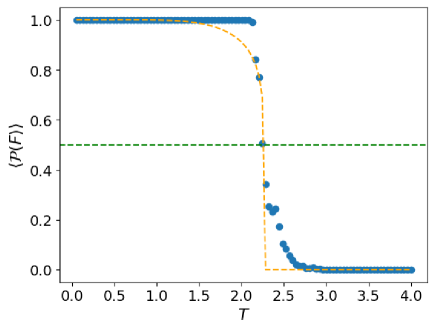
The first notable feature is that ${\left<{\mathcal{P}{\left(F\right)}}\right>}$ follows closely the magnetization at the training temperatures and has a transition almost at the same point, even not being trained with information in its direct neighborhood. This is a general feature, with tests showing that changing sensibly the activation function can improve the coincidence, although it does not have a significant effect in the final estimation of $T_{c}$. In particular, one can see how the point where the probability falls to 1/2 approximates well the critical temperature. Although that is not explicit in that work, the data collapse used to pinpoint the critical temperature in [2] shows a crossing of the plots that visually coincides with an output equals to 1/2 of the used NN with one hidden layer, which is exactly its decision boundary.

For a linear classifier as the SLNN, the decision boundary is the value of $s$ that solves the equation $x\equiv w\cdot s+w_{0}=0$, where $x$ is the argument of the activation function. Because the symmetry of the lattice with PBCs implies that all sites should contribute equally to the classification, on average all coordinates of $w$ should be equal. This will not happen in practice due to the stochastic nature of the training, but if one considers the asymptotic average scenario, one can predict that the solution should approximate $w_{i}=\bar{w}$, $\forall i$, leading to $x=\bar{w}Nm+w_{0}$.

Figure 2 shows a scatter plot of all values of the magnetization $m(s)$ for one single test set (chosen arbitrarily) against the corresponding values of the dot product $w\cdot s$ divided by its maximum value over the set. It is clear from the plot that, although not perfectly, the parameters are indeed fitting the magnetization, apart from a multiplicative constant.

Figure 2: Scatter plot showing the almost perfect positive correlation between the magnetization of the spin configurations $s$ and the scaled value of the products $w\cdot s$.

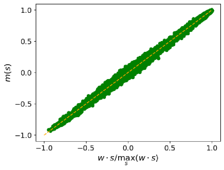
Figure 3 reveals yet another piece of information needed to understand the strategy of the model.

Figure 3: Upper plot: argument of the sigmoid for each configuration in the test set; lower plot: probability of the configuration belonging to the ferromagnetic phase.

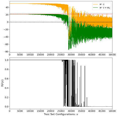
The upper plot shows the value of $w\cdot s$ (orange) and that of $x$ (green). The upper (red) dashed line shows the difference between the maximum value of the former and that of the latter. The lower plot is the probability of the corresponding configuration being in the ferromagnetic phase.

The plots clearly show how the network is working. It first scales up the values of the magnetization by a factor large enough such that the sigmoid’s argument $x$ becomes largely negative at low temperatures, bringing the calculated probability of the ferromagnetic very close to 1. In order to fit a zero probability for the paramagnetic phase, $w_{0}$ becomes negative enough to bring all configurations with magnetization in the training range below zero, but still not enough to spoil the fitting of the ferromagnetic phase. This is achieved, in all observed training, by using a value $w_{0}$ about half of the maximum $x$. In the region close to the critical temperature, the network simply uses the statistics of the magnetizations learned from the trained intervals. As it depends only on the statistics of the magnetization, the same strategy should allow the network to infer the critical temperature for any lattice – which indeed seems to happen.

The fact that the SLNN is a linear classifier allows for a geometric interpretation of the result. It works by finding the best separating hyperplane between the two classes, in this case the ferro and paramagnetic phases. For the ferromagnetic Ising model, the training rotates the normal to this plane, which is $w$, until it is aligned to the direction of the magnetization. Previous studies using principal component analysis (PCA) [1], a linear clustering method, have shown that this is the direction of the largest variance of the magnetization for the configurations, as the inter-class variance should be larger than the intra-class one. When trained with positive magnetizations above the critical temperature, as is the case here, the SLNN adjusts the origin of the separating hyperplane such that all configurations in the training set that are in the paramagnetic phase will lie under the plan (in the opposite direction of $w$) having then a probability less than 1/2 of being ferromagnetic. If the distance to the plane is large enough, the scaling stretches it such that it becomes effectively 1 above it and 0 below.

The reason a linear model classifier trained at extreme temperatures in one lattice can infer the critical temperature for the others, even when only a sample of each configuration is used and the topology is ignored in the inputs is that, as mentioned, the ferromagnetic transition depends only on the value of the magnetization, which is linear and local.

Unsurprisingly, if the training is done with the MH algorithm allowing negative magnetizations in the ferromagnetic phase, the SLNN will not be able to learn the classification as one single plane cannot separate the two phases in the configuration space. On the axis of the magnetization, the configurations with high probability of being ferromagnetic occupy the regions closer to the values $\pm 1$, with the paramagnetic ones located in a cluster between these two. However, this picture implies that two such planes aligned with the magnetization axis should be enough if their classifications are properly combined. This explains why the 1HLNN with only two units used in [19] is effective in solving the problem. Each unit in a hidden layer works as a separate SLNN with the same input vector, allowing for the segmentation of the space by several planes. By using the understanding obtained with the simpler model, one can then fact predict the minimum value of a hyperparameter, namely the number of hidden units, necessary to find the correct solution.

By analyzing the solution of such a 1HLNN with two units, it is possible, once again, to explain how it obtains the solution. Both the training and test sets where now generated by MH with ferromagnetic configurations allowed to have negative magnetizations. Figure 4 show the average probability of being in the ferromagnetic state over 20 test sets.

Figure 4: Same plot as in figure 1, but now for the 1HLNN with two hidden units and trained without restrictions on the sign of the magnetization.

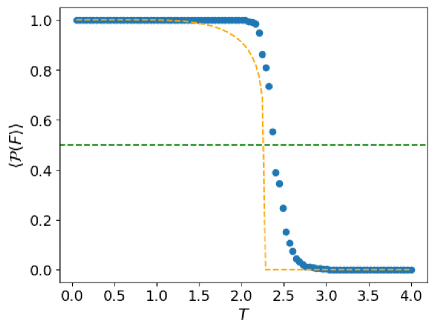
Although less closely, the average probability for the ferromagnetic phase still follows the magnetization for the infinite lattice. The critical temperature is not as well approximated, but although this could be improved as shown in [19], this will not be done here as the aim is to explain the inferred result, not to actually calculate $T_{c}$. For this particular instance of training, figure 5 allows us to understand the strategy used by the network to carry out the classification.

Figure 5: Probabilities inferred by the first (blue) and second (red) units of the hidden layers of the 1HLNN, together with the final probability for the input configuration to be in the ferromagnetic case (green) plotted against the magnetization values of the configurations. The plot shows the average over 500 random configurations for each value of the magnetization.

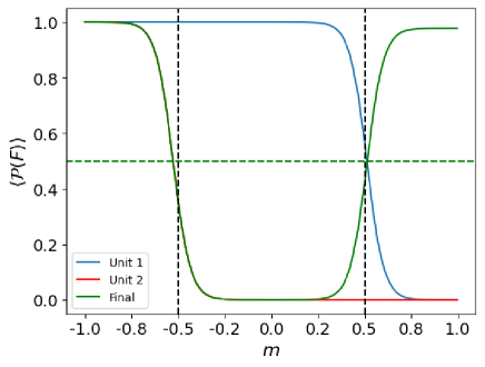
The plot is obtained by generating 500 random configurations for each value of the magnetization and then observing the outputs of each of the network’s layers on them. The result is then averaged and plotted. The second unit in the hidden layer, the inference of which is given by the red line only partially visible as its first part is hidden by the green line, clearly specializes in the negative magnetizations. The separating hyperplane is located close to a magnetization of -0.5 and magnetizations below that have a probability above 1/2 of being ferromagnetic according to this unit, while those above it are classified as paramagnetic. The behavior of the first unit, represented by the blue line, is more interesting. It actually exchanges the ferromagnetic by the paramagnetic phase. The separating hyperplane is located close to magnetization 0.5, but it gives magnetizations above that a larger probability of being paramagnetic. This “mistake” is however corrected by the final output layer, and the final classification, green line, provides a probability profile as it one would expect.

The exchanged classification of the first hidden unit is not in fact a mistake. This unit has no direct access to the labels during the training. This information is passed to it only by the final (output) layer through backpropagation. The unit ends up using the opposite labeling convention from the other, but that is compensated by the output layer which has direct knowledge of the correct labels. It is possible to observe, by repeating the training several times, that all four combinations of label attributions by the hidden units can happen, with the final classification always being corrected by the output layer.

The way the output layer combine the probabilities, compensating for any difference in labeling by the hidden units, is deceptively simple. There are only three parameters in this layer, the weights from hidden units 1 and 2 and the bias. For the particular result shown in figure 5 for instance, these numbers are $w_{1}\approx-26.633$, $w_{2}\approx 27.232$and $w_{0}\approx 13.097$, respectively. It is not difficult to convince oneself that the output of the network is obtained by simply rescaling appropriately the combination $-{\mathcal{P}{\left(F\right)}}_{1}+{\mathcal{P}{\left(F\right)}}_{2}+1/2$, which is the simplest algebraic expression that will provide a good approximation for the classification. For all observed training sessions, although the rescaling changes, the strategy of using this simple algebraic expression is always used by the output layer.

It is worth mentioning that the 1HLNN with two units is also capable of finding the critical temperature of the anti-ferromagnetic Ising model using the same strategy when trained with data from that version of the model. The only difference is that the normal to the separating hyperplanes is now in the direction of the staggered magnetization, i.e., the sum of the magnetizations of the two square sublattices with opposite signs. All else remains the same. These results, not shown here, can easily be obtained simply by using $J=-1$ when generating the training and test sets.

The explanation of the ML solution for the ferromagnetic Ising model provided here does not invalidate or diminish any of the previous results. Instead, it corroborates them by showing that one can indeed understand their inner workings. The explanation of the strategies used by simpler ML models indicate the directions that can be taken in order to fully explain those of the more sophisticated ones, opening the ML black-boxes. In addition, it also indicates the possible paths to address statistical physics systems with phase transitions with even more phases and more involved order parameters. From the analysis presented here, the presence of more phases clearly requires a corresponding increase in the number of hidden units of the NNs. Depending on the geometry of the corresponding clusters of configurations, kernel techniques [24] might help decrease the complexity of the required architectures. On the other hand, hidden order parameters might require extra layers, while topological phase transitions might require the use of CNNs as the lattices would need to be considered as whole “images”. Finally, extensions of the work presented in this letter are currently being applied to the study of other statistical physics models with more general phase transitions, both classical and quantum. While it has not yet been possible to extract physical laws from the inferred parameters, this remains one of the main objectives of this research.