Learning the Topology and Behavior of Discrete
Dynamical Systems

Abstract

Discrete dynamical systems are commonly used to model the spread of contagions on real-world networks. Under the PAC framework, existing research has studied the problem of learning the behavior of a system, assuming that the underlying network is known. In this work, we focus on a more challenging setting: to learn both the behavior and the underlying topology of a black-box system. We show that, in general, this learning problem is computationally intractable. On the positive side, we present efficient learning methods under the PAC model when the underlying graph of the dynamical system belongs to some classes. Further, we examine a relaxed setting where the topology of an unknown system is partially observed. For this case, we develop an efficient PAC learner to infer the system and establish the sample complexity. Lastly, we present a formal analysis of the expressive power of the hypothesis class of dynamical systems where both the topology and behavior are unknown, using the well-known formalism of the Natarajan dimension. Our results provide a theoretical foundation for learning both the behavior and topology of discrete dynamical systems.

Conference version. The conference version of the paper is accepted at AAAI-2024.

1 Introduction

Discrete dynamical systems are formal models for numerous cascade processes, such as the spread of social behaviors, information, diseases, and biological phenomena [6, 19, 9, 14, 23, 25]. A discrete dynamical system consists of an underlying graph with vertices representing entities (e.g., individuals, genes), and edges representing connections between the entities. Further, each vertex has a contagion state and an interaction function (i.e., behavior), which specify how the state changes over time. Overall, vertices update states using interaction functions as the system dynamics proceeds in discrete time.

Due to the large scale of real-world cascades, a complete specification of the underlying dynamical system is often not available. To this end, learning the unknown components of a system is an active area of research [3, 8, 10, 12]. One ongoing line of work is to infer the unknown interaction functions or the topology of a system. Interaction functions and the network topology play critical roles in the system dynamics. The topology encodes the underlying relationships between the entities, while the interaction functions provide the decision rules that entities employ to update their contagion states. The class of threshold interaction functions [16], which are widely used to model the spread of social contagions [31], is one such example. Specifically, each entity in the network has a decision threshold that represents the tipping point for a behavioral (i.e., state) change. In the case of a rumor, a person’s belief shifts when the number of neighbors believing in the rumor reaches a certain threshold.

Previous research [2] has presented efficient algorithms for inferring classes of interactions functions (e.g., threshold functions) based on the observed dynamics, assuming that the underlying network is known. To our knowledge, the more challenging problem of learning a system from observed dynamics, where both the interaction function and the topology are unknown, has not been examined. In this work, we fill this gap with a theoretical study of the problem of learning both the network and the interaction functions of an unknown dynamical system.

Problem description. Consider a black-box networked system where both the interaction functions and the network topology are unknown. Our objective is to recover a system that captures the behavior of the true but unknown system while providing performance guarantees under the Probably Approximately Correct (PAC) model [29]. We learn from snapshots of the true system’s dynamics, a common scheme considered in related papers (e.g., [7, 10, 33]). Since our problem setting also involves multiclass learning, we examine the Natarajan dimension [21], a well-known generalization of the VC dimension [30]. In particular, the Natarajan dimension quantifies the expressive power of the hypothesis class and characterizes the sample complexity of learning. Overall, we aim to answer the following two questions: $(i)$ Can one efficiently learn the black-box system, and if so, how many training examples are sufficient? $(ii)$ What is the expressive power of the hypothesis class of networked systems?

The key challenges of our learning problem arise from the incomplete knowledge of the network topology and the interaction functions of the nodes in the system. For example, when we consider systems whose underlying graphs are undirected and the interaction functions are Boolean threshold functions, the number of potential systems is $\Theta(2^{\binom{2}{2}}\cdot n^{n})$, where $n$ is the number of nodes in the underlying graph. Therefore, a learner needs to find an appropriate hypothesis in a very large space. Further, in general, the training set (which consists of snapshots of the system dynamics) may not contain sufficient information to recover the underlying network structure efficiently (as we show that the problem is computationally intractable). Our main contributions are summarized below.

1. Hardness of PAC learning:  We show that in general, hypothesis classes corresponding to dynamical system, where both the network topology and the interaction functions are unknown, are not efficiently PAC learnable unless $\textbf{NP}=\textbf{RP}$. We prove this result by first formulating a suitable decision problem and showing that the problem is NP-complete. We use the hardness result for the decision problem to establish the hardness of PAC learning. Our results show that the learning problem remains hard for several classes of dynamical systems (e.g., systems on undirected graphs with threshold interaction functions).

2. Efficient PAC learning algorithms for special classes.  In contrast with the general hardness result above, we identify some special classes of systems which are efficiently PAC learnable. The two classes that we identify correspond to systems on directed graphs with bounded indegree and those where underlying graph is a perfect matching. In both cases, the interaction functions are from the class of threshold functions. These results are obtained by showing that these systems have efficient consistent learners and then appealing to the known result [27] that hypothesis classes for which there are efficient consistent learners are also efficiently PAC learnable.

3. Learning under a relaxed setting.  We consider a relaxed setting where the underlying network is partially observed. Towards this end, we present an efficient PAC learner and establish the sample complexity of learning under this setting.

4. Expressive power.  We present an analysis of the Natarajan dimension (Ndim), which measures the expressive power of the hypothesis class of networked systems. In particular, we give a construction of a shatterable set and prove that the Ndim of the hypothesis class is at least $\lfloor n^{2}/4\rfloor$, where $n$ is the number of vertices. Further, we show that the upper bound on the Ndim is $O(n^{2})$. Thus, our lower bound is tight to within a constant factor. Our result also provides a lower bound on the sample complexity.

Related work. Learning unknown components of networked systems is an active area of research. Many researchers have studied the problem of identifying missing components (e.g., learning the diffusion functions at vertices, edge parameters, source vertices, and contagion states of vertices) in contagion models by observing the propagation dynamics. For instance, Chen et al. [7] infer the edge probability and source vertices under the independent cascade model. Conitzer et al. [10] investigate the problem of inferring opinions (states) of vertices in stochastic cascades under the PAC scheme. Lokhov [20] studies the problem of reconstructing the parameters of a diffusion model given infection cascades. Inferring threshold functions of vertices from social media data is also considered in [14, 23]. Learning the source vertices of infection for contagion spreading is addressed in [34, 26]. The problem of inferring the network structure has also been studied, see, for example [18, 22, 1, 13, 28]. The problem of inferring the network structure and the interaction functions of dynamical systems has been studied under a different model in [24], where a user can submit queries to the system and obtain responses. This is very different from our model where a learning algorithm must rely on a given set of observations and cannot interact with the unknown system.

The work that is closest to ours is [2], where the problem of inferring the interaction functions in a system from observations is considered, under the assumption that the network is known. For the type of observations used in our paper, it is shown in [2] that the local function inference problem can be solved efficiently. However, the techniques used in [2] are not applicable to our context, since the network is unknown.

2 Preliminaries

2.1 Discrete Dynamical Systems

A Synchronous Dynamical System (SyDS) $\mathcal{S}$ over the Boolean domain $\mbox{$\mathbb{B}$}{}=\{0,1\}$ is a pair ${\cal S}=(\mathcal{G},{\cal F})$, where:

• $\mathcal{G}{}=(\mathcal{V}{},\mathcal{E}{})$ is the underlying undirected graph. We let $n=|\mathcal{V}{}|$. Each vertex in $\mathcal{V}{}$ has a state from $\mathbb{B}$, representing its contagion state (e.g., inactive or active).

• ${\cal F}=\{f_{1},f_{2},\ldots,f_{n}\}$ is a collection of functions, where $f_{i}$ is the interaction function of vertex $v_{i}\in\mathcal{V}{}$, $1\leq i\leq n$.

Interaction functions. The system evolves in discrete time steps, with vertices updating their states synchronously using the interaction functions. For a graph $\mathcal{G}{}$ and a vertex $v$, we let $N(\mathcal{G}{},v)$ and $N^{+}(\mathcal{G}{},v)$ denote the open and closed neighborhoods of $v$, respectively. At each time step, the inputs to the interaction function $f_{i}\in\mathcal{F}$ are the states of the vertices in $N^{+}(\mathcal{G}{},v_{i})$; $f_{i}$ computes the next state of $v_{i}$.

Our work focuses on the class of threshold interaction functions, which is a classic framework modeling the spread of social contagions [32, 16]. Specifically, each vertex $v_{i}\in\mathcal{V}{}$ has an integer threshold $\tau_{v_{i}}\geq 0$, and $f_{i}$ outputs $1$ if the number of 1’s in the input to $f_{i}$ (i.e., the number of state-1 vertices in $v_{i}$’s closed neighborhood) is at least $\tau_{v_{i}}$; $f_{i}$ outputs $0$ otherwise. An example of a SyDS is shown in Figure 1.

A configuration $\mathcal{C}$ of a SyDS $\mathcal{S}$ at a given time step is a binary vector of length $n$ that specifies the states of all the vertices at that time step. Let $\mathcal{X}=\{0,1\}^{n}$ be the set of all configurations. For a given vertex $v$, let $\mbox{$\mathcal{C}$}(v)$ denote the state of $v$ in $\mathcal{C}$, and for a given vertex set $\mathcal{Y}\subseteq\mathcal{V}{}$, let $\mbox{$\mathcal{C}$}[\mathcal{Y}]$ denote the projection of $\mathcal{C}$ onto $\mathcal{Y}$. If the system $\mathcal{S}$ evolves from $\mathcal{C}$ to a configuration $\mbox{$\mathcal{C}$}{}^{\prime}$ in one step, denoted by $\mathcal{S}(\mathcal{C})=\mbox{$\mathcal{C}$}{}^{\prime}$, then $\mbox{$\mathcal{C}$}{}^{\prime}$ is called the successor of $\mathcal{C}$. Since the interaction functions considered in our work are deterministic, each configuration has a unique successor. For a given configuration $\mathcal{C}$ and a vertex set $\mathcal{Y}$, we let $score(\mbox{$\mathcal{C}$},\mathcal{Y})$ denote the number of vertices $v\in\mathcal{Y}$ such that $\mbox{$\mathcal{C}$}(v)=1$.

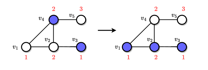
Figure 1: An example of a single transition of a SyDS with threshold interaction functions. The threshold values of vertices are highlighted in red. State-1 vertices are in blue.

SyDSs over directed graphs. SyDSs can also be defined over directed graphs. In such a case, the inputs to the local function at a vertex $v_{i}$ are the state of $v_{i}$ and those of the in-neighbors of $v_{i}$ (i.e., vertices from which $v_{i}$ has incoming edges). All the other definitions for SyDSs on directed graphs are the same as those for SyDSs on undirected graphs. In this paper, we assume that the underlying graph is undirected, unless specified otherwise.

2.2 The Learning Problem

Hypotheses. Let ${\cal S}^{*}=(\mathcal{G}{},{\cal F})$ be a ground truth SyDS. The learner does not know either the graph $\mathcal{G}{}$ or the set of functions ${\cal F}$. Other than the training set, the only information provided to the learner consists of the number $n$ of vertices, the class of interaction functions, and the class of the underlying graph. The learner must find a hypothesis consisting of an underlying graph (from the given graph class) and an interaction function (from the given class of interaction functions) for each node of the graph from the set of all such hypotheses. As an illustration, let $\mathcal{H}{}$ denote the hypothesis class where the underlying graph of ${\cal S}^{*}$ is undirected, and the interaction functions are threshold functions. Since there are $2^{\binom{n}{2}}$ undirected graphs with $n$ nodes and each node may have $\Theta(n)$ choices for threshold values, the hypothesis class $\mathcal{H}{}$ has $\Theta(2^{\binom{n}{2}}n^{n})$ systems (i.e., hypotheses). The learner aims to infer a system $\mathcal{S}\in\mathcal{H}{}$ that is close to the true system $\mathcal{S}^{*}$ by recovering the graph and the interaction functions of $\mathcal{S}$.

Learning setting. Our algorithms learn the ground truth system ${\cal S}^{*}$ from its observed dynamics. Let $\mbox{$\mathbb{O}$}{}=\{(\mathcal{C}_{i},\mathcal{C}^{\prime}_{i})\}_{i=1}^{q}$ be a training set of $q$ examples, which consists of the snapshots of the dynamics of ${\cal S}^{*}$ in the form of configuration-successor pairs. Specifically, $\mathcal{C}_{i}$ is a drawn i.i.d. from a distribution (unknown to the learner) $\mathcal{D}$ over $\mathcal{X}$, and $\mathcal{C}_{i}^{\prime}=\mathcal{S}^{*}(\mathcal{C}_{i})$ is the successor of $\mathcal{C}_{i}$ under $\mathcal{S}^{*}$. Let $\mbox{$\mathbb{O}$}\sim\mathcal{D}^{q}$ denote such a training set. We say that a hypothesis $\mathcal{S}$ is consistent with $\mathbb{O}$ if $\forall(\mathcal{C}_{i},\mathcal{C}_{i}^{\prime})\in\mbox{$\mathbb{O}$}{}$,  $\mathcal{S}(\mathcal{C}_{i})=\mathcal{C}_{i}^{\prime}$. For each vertex $v\in\mathcal{V}{}$, we define a partition of $\mathbb{O}$ into two subsets $\{\mbox{$\mathbb{O}$}{}_{0,v},\mbox{$\mathbb{O}$}{}_{1,v}\}$, such that $\mathcal{C}^{\prime}(v)=i$, for all $(\mathcal{C},\mathcal{C}^{\prime})\in\mbox{$\mathbb{O}$}{}_{i,v}$, $i=0,1$. Note that in general, the hypothesis being learned is a successor function.

For simplicity, we present the necessary definitions for the PAC model (see e.g., [27]) using $\mathcal{H}{}$. These definitions also apply to other hypothesis classes considered in this paper. The true error of a hypothesis $\mathcal{S}\in\mathcal{H}{}$ is defined as $L_{(\mathcal{D},\mathcal{S}^{*})}(\mathcal{S}):=\Pr{}_{\mathcal{C}\sim\mathcal{D}}[\mathcal{S}(\mathcal{C})\neq\mathcal{S}^{*}(\mathcal{C})]$. In the PAC model, the goal is to infer a hypothesis $\mathcal{S}\in\mathcal{H}{}$ s.t. with probability at least $1-\delta$ over $\mbox{$\mathbb{O}$}{}\sim\mathcal{D}^{q}$, the true error $L_{(\mathcal{D},\mathcal{S}^{*})}(\mbox{$\mathbb{O}$}{})\leq\epsilon$, for any given $\epsilon,\delta\in(0,1)$. The class $\mathcal{H}$ is efficiently PAC learnable if such an $\mathcal{S}\in\mathcal{H}{}$ can be inferred in polynomial time (w.r.t. $n$, $1/\delta$ and $1/\epsilon$). The minimum number of training examples needed to achieve the above guarantee is called the sample complexity of learning $\mathcal{H}{}$.

Natarajan dimension. A hypothesis $\mathcal{S}$ can be viewed as a function $\mathcal{X}\rightarrow\mathcal{X}$, where each of the $2^{n}$ possible target configurations is considered a class. Thus, our learning problem involves multiclass classification. The Natarajan dimension [21] is a generalization of the concept of VC dimension to a multiclass setting, and measures the expressive power of a given hypothesis class $\mathcal{H}{}$. Formally, a set $\mathcal{R}$ of configurations is shattered by $\mathcal{H}{}$ if there exists two functions $g_{1},g_{2}:\mathcal{X}\rightarrow\mathcal{X}$, such that: $(i)$ for every $\mathcal{C}\in\mathcal{R}$, $g_{1}(\mathcal{C})\neq g_{2}(\mathcal{C})$, and $(ii)$ for every subset $\mathcal{R}^{\prime}\subseteq\mathcal{R}$, there exists $\mathcal{S}\in\mathcal{H}{}$ such that $\forall\mathcal{C}\in\mathcal{R}^{\prime},\;\mathcal{S}(\mathcal{C})=g_{1}(\mathcal{C})$ and $\forall\mathcal{C}\in\mathcal{R}\setminus\mathcal{R}^{\prime},\;\mathcal{S}(\mathcal{C})=g_{2}(\mathcal{C})$. The Natarajan dimension of $\mathcal{H}{}$, denoted by $\text{Ndim}(\mathcal{H}{})$, is the maximum size of a shatterable set. In general, the larger the Natarajan dimension of a hypothesis class, the higher its expressive power.

3 PAC Learnability and Sample Complexity

We first establish the intractability of efficiently PAC learning threshold dynamical systems over general graphs. We then present efficient algorithms for learning systems over several graph classes. We also analyze the sample complexity of learning the corresponding hypothesis classes.

3.1 Intractability of PAC learning

To establish the hardness of learning, we first formulate a decision problem for SyDSs and show that the problem is NP-hard. We use this to establish a general hardness result under the PAC model. We define restricted classes of SyDSs by specifying constraints on the underlying graph and the interaction functions. For example, we use the notation (Undir, Thresh)-SyDSs to denote the restricted class of SyDSs whose $(i)$ underlying graphs are undirected and $(ii)$ interaction functions are threshold functions. Several other restricted classes of SyDSs will be considered in this section.

Given a set $\mathbb{O}$ of observations, with each observation being a pair of the form $(\mbox{$\mathcal{C}$}{},\mbox{$\mathcal{C^{\prime}}$}{})$ where $\mathcal{C^{\prime}}$ is the successor of $\mathcal{C}$, we say that a SyDS $\mathcal{S}$ is consistent with $\mathbb{O}$ if for each observation $(\mbox{$\mathcal{C}$},\mbox{$\mathcal{C^{\prime}}$})\in\mbox{$\mathbb{O}$}$, the successor of $\mathcal{C}$ produced by $\mathcal{S}$ is $\mathcal{C^{\prime}}$. A basic decision problem in this context is the following: given a set $\mathbb{O}$ of observations, determine whether there is a SyDS that is consistent with $\mathbb{O}$. One may also want the consistent SyDS to be in a restricted class $\Gamma$. We refer to this problem as the $\Gamma$-Consistency problem:

$\Gamma$-Consistency

Instance: A vertex set $\mathcal{V}{}$ and a set of observations $\mathbb{O}$ over $\mathcal{V}{}$.

Question: Is there a SyDS in the class $\Gamma$ that is consistent with $\mathbb{O}$?

Hardness. The following lemma shows the hardness of $\Gamma$-consistency for two restricted classes of SyDSs:

$(i)$ (Undir, Thresh)-SyDSs, where the graph is undirected and each interaction function is a threshold function.

$(ii)$ (Tree, Thresh$\,=2$)-SyDSs, where the graph is a tree and each interaction function is a 2-threshold function. A full proof of the lemma appears in the appendix.

Lemma 3.1.

The $\Gamma$-Consistency problem is NP-complete for the following classes of SyDSs: $(i)$ (Undir, Thresh)-SyDSs and $(ii)$ (Tree, Thresh$\,=2$)-SyDSs.

Proof sketch for $(i)$:  It can be seen that the problem is in NP. The proof of NP-hardness is via a reduction from 3SAT. Let the given 3SAT formula be $f$, with variables $X=\{x_{1}.\ldots,x_{n}\}$ and clauses $C=\{c_{1}.\ldots,c_{m}\}$. For the reduction, we construct a node set $V$ and transition set $\mathbb{O}$.

The constructed node set $V$ contains $2n+2$ nodes. For each variable $x_{i}\in X$, $V$ contains the two nodes $y_{i}$ and $\overline{y_{i}}$. Intuitively, node $y_{i}$ corresponds to the literal $x_{i}$, and node $\overline{y_{i}}$ corresponds to the literal $\overline{x_{i}}$. We refer to these $2n$ nodes as literal nodes. There are also two additional nodes: $z$ and $z^{\prime}$. Transition set $\mathbb{O}$ contains $n+m+2$ transitions, as follows: $\mbox{$\mathbb{O}$}{}=\mbox{$\mathbb{O}$}{}^{1}\cup\mbox{$\mathbb{O}$}{}^{2}\cup\mbox{$\mathbb{O}$}{}^{3}$.

$\mbox{$\mathbb{O}$}{}^{1}$ contains two transitions. In the first of these transitions, the predecessor has only node $z$ equal to 1, and the successor has all nodes equal to 0. In the second transition, the predecessor has only the two nodes $z$ and $z^{\prime}$ equal to 1, and the successor has only node $z$ equal to 1. $\mbox{$\mathbb{O}$}{}^{2}$ contains $n$ transitions, one for each variable in $X$. For each variable $x_{i}\in X$, $\mbox{$\mathbb{O}$}{}^{2}$ contains a transition where in the predecessor only nodes $y_{i}$ and $\overline{y_{i}}$ are equal to 1, and the successor has all nodes equal to 0. $\mbox{$\mathbb{O}$}{}^{3}$ contains $m$ transitions, one for each clause of $f$. For each clause $c_{j}$ of $f$, $\mbox{$\mathbb{O}$}{}^{3}$ contains a transition where in the predecessor only node $z$ and the nodes corresponding to the literals that occur in $c_{j}$ are equal to 1, and the successor has only node $z$ equal to 1. The construction can be done in polynomial time. It can be shown that $f$ is satisfiable iff there exists a threshold-SyDS that is consistent with $\mathbb{O}$.  

Remark. The usefulness of establishing NP-hardness results for the $\Gamma$-Consistency problem is pointed out by the next Lemma 3.2, which states that if $\Gamma$-Consistency is NP-hard, then the hypothesis class for $\Gamma$ SyDSs is not efficiently PAC learnable. In the statement of the result, RP denotes the class of problems that can be solved in randomized polynomial time. It is widely believed that the complexity classes NP and RP are different; see [5] for additional details regarding these complexity classes.

Lemma 3.2.

Let $\Gamma$ be any class of SyDS for which $\Gamma$-Consistency is NP-hard. The hypothesis class for $\Gamma$ SyDSs is not efficiently PAC learnable, unless NP = RP.

Proof sketch. If the hypothesis class for $\Gamma$-SyDS admits an efficient PAC learner $\mathcal{A}_{\textsf{PAC}}$, then one can construct an RP algorithm $\mathcal{A}_{\textsf{ERM}}$ (based on $\mathcal{A}_{\textsf{PAC}}$) for the $\Gamma$-Consistency problem, thereby implying NP = RP. Details of the proof appear in the appendix.  

We now present the theorem on the hardness of learning, which is a direct consequence of Lemmas 3.1 and 3.2.

Theorem 3.3.

Unless NP = RP, the hypothesis classes for the following classes of SyDSs are not efficiently PAC learnable: $(i)$ (Undir, Thresh)-SyDSs and $(ii)$ (Tree, Thresh$\,=2$)-SyDSs.

Sample complexity. For any finite hypothesis class $H$, given the PAC parameters $\epsilon,\delta>0$, the following is a well known [17] upper bound on the sample complexity $m_{H}(\delta,\epsilon)$ for learning $H$: $m_{H}(\delta,\epsilon)\leq\frac{1}{\epsilon}\big{(}\log(|H|+\log(1/\delta)\big{)}$. As mentioned earlier, the size of the hypothesis class $\mathcal{H}{}$ is $O(2^{\binom{n}{2}}\cdot n^{n})$. Thus, one can obtain an upper bound on the sample complexity of learning $\mathcal{H}{}$:

$$m_{\mathcal{H}{}}(\delta,\epsilon)\leq\frac{1}{\epsilon}\cdot\left(n^{2}+n\log{}(n)+\log{}(\frac{1}{\delta})\right)$$ (1)

From the above inequality, it follows that $m_{\mathcal{H}{}}(\delta,\epsilon)=O\left((1/\epsilon)\cdot(n^{2}+\log{}(1/\delta))\right)$. In a later section, we will prove a lower bound on the sample complexity which is tight to within a constant factor from the upper bound (1), thereby showing that $m_{\mathcal{H}{}}(\delta,\epsilon)=\Theta\left((1/\epsilon)\cdot(n^{2}+\log{}(1/\delta))\right)$.

Preview for the results in Sections 3.2 and 3.3.  In the next subsections, we present classes of SyDSs which are efficiently PAC learnable. In both cases, we obtain the result by showing that for the corresponding class of SyDSs, the $\Gamma$-Consistency problem is efficiently solvable. In other words, given a training set $\mathbb{O}$, these algorithms represent efficient consistent learners for the corresponding classes of SyDSs. As is well known, an efficient consistent learner for a hypothesis class is also an efficient PAC learner [27].

3.2 PAC Learnability for Matchings

Let (Match,Thresh)-SyDSs denote the set of SyDSs where the underlying graph is a perfect matching, and the interaction functions are threshold functions. In this section, we present an efficient PAC learner for the hypothesis class $\mathcal{H}_{\textsc{match}}{}$, consisting of (Match,Thresh)-SyDSs. As mentioned earlier, we obtain an efficient PAC learner for this class by presenting an efficient algorithm for the $\Gamma$-Consistency problem. We begin with a few definitions.

Threshold-Compatibility. For a pair of distinct vertices $u$ and $v$, we say that $u$ and $v$ are threshold-compatible if for all $(C_{i},C_{i}^{\prime})$ and $(C_{j},C_{j}^{\prime})\in\mbox{$\mathbb{O}$}$, if $score(C_{i},\{u,v\})\leq score(C_{j},\{u,v\})$, then $C_{i}^{\prime}(u)\leq C_{j}^{\prime}(u)$ and $C_{i}^{\prime}(v)\leq C_{j}^{\prime}(v)$. Informally, $u$ and $v$ are threshold-compatible iff there exist functions $f_{u}$ for $u$ and $f_{v}$ for $v$, each of which is a threshold function of $u$ and $v$, such that $f_{u}$ and $f_{v}$ are each consistent with $\mathbb{O}$.

Compatibility Graph. The threshold-compatibility graph $\mathcal{G}{}^{\prime}=(\mathcal{V},\mathcal{E}^{\prime})$ of $\mathbb{O}$ is an undirected graph with vertex set $\mathcal{V}{}$, and an edge $(u,v)\in\mathcal{E}^{\prime}$ for each pair of threshold-compatible vertices $u$ and $v$.

Input : The vertex set $\mathcal{V}{}$; A training set $\mathbb{O}$

1

Output :  An (Undir, Thresh)-SyDSs SyDS $\mathcal{S}=(G,\mathcal{F})$

2

3Construct the threshold-compatibility graph $\mathcal{G}{}^{\prime}=(\mathcal{V},\mathcal{E}^{\prime})$ of $\mathbb{O}$

4If $\mathcal{G}{}$ does not have a perfect matching, answer “No” and stop.

5Let $\mathcal{E}^{\prime\prime}$ be the edge set of a perfect matching in $\mathcal{G}{}$.

6$G\leftarrow(\mathcal{V},\mathcal{E}^{\prime\prime})$; $\mathcal{F}=\emptyset$

7

8for each $v\in\mathcal{V}{}$ do

9        if $|\mbox{$\mathbb{O}$}_{1,v}|=0$ then

10               $f_{v}\leftarrow$ the threshold function where $\tau_{v}=3$

11              

12       else

13               let $u$ be the neighbor of $v$ in $G$

14              $z\leftarrow$ the minimum value of $score(C,\{u,v\})$ over all $(C,C^{\prime})\in\mbox{$\mathbb{O}$}_{1,v}$

15              $f_{v}\leftarrow$ the threshold function where $\tau_{v}=z$

16        end if

17       $\mathcal{F}\leftarrow\mathcal{F}\cup\{f_{v}\}$

18 end for

19return $\mathcal{S}=(G,\mathcal{F})$

Algorithm 1 Full-Infer-Matching($\mathcal{V}{}$)

An efficient learner. Our efficient algorithm for the $\Gamma$-Consistency problem for the class of (Match,Thresh)-SyDSs appears as Algorithm 1. The algorithm first constructs the threshold-compatibility graph $\mathcal{G}{}^{\prime}=(\mathcal{V},\mathcal{E}^{\prime})$ of $\mathbb{O}$. The reason for this computation is given in the following lemma (proof in Appendix).

Lemma 3.4.

The answer to the $\Gamma$-Consistency problem for (Match,Thresh)-SyDSs is “Yes” if and only if the threshold-compatibility graph $\mathcal{G}{}^{\prime}=(\mathcal{V},\mathcal{E}^{\prime})$ of $\mathbb{O}$ contains a perfect matching.

Next, the algorithm finds a maximum matching in $\mathcal{G}{}^{\prime}$. Let $\mathcal{E}^{\prime\prime}$ be the edge set of this maximum matching. Note that, from Lemma 3.4, $\mathcal{G}{}^{\prime}$ contains a perfect matching, so $\mathcal{E}^{\prime\prime}$ is a perfect matching of $\mathcal{G}$. The learned hypothesis $\mathcal{S}$ is a (Match,Thresh)-SyDSs on $\mathcal{V}{}$ whose graph has edge set $\mathcal{E}^{\prime\prime}$, and interaction function $f_{v}$ for each vertex $v$, with incident edge $(v,u)$ in $\mathcal{E}^{\prime\prime}$, is any threshold function of variables $v$ and $u$ that is consistent with $\mbox{$\mathbb{O}$}[\{v,w\}]$.

Remark. To estimate the running time of Algorithm 1, note that for any pair of nodes, determining compatibility can be done in $O(nq)$ time, where $n$ is the number of nodes and $q$ is the number of given observations. Thus, the time to construct the compatibility graph is $O(n^{3}q)$. All the other steps (including the computation of perfect matching which can be done in $O(n^{3})$ time [11]) are dominated by the time to construct the compatibility graph. Thus, the overall running time is $O(n^{3}q)$, which is polynomial in the input size. Hence, we have an efficient consistent learner for the class of (Match,Thresh)-SyDSs.

Theorem 3.5.

The hypothesis class associated with (Match,Thresh)-SyDSs is efficiently PAC learnable.

3.3 PAC Learnability for Directed Graphs

In this section, we present an efficient PAC learner for the hypothesis class $\mathcal{H}_{\textsc{dir,$\Delta$}-\textsc{bounded}}{}$ consisting of SyDSs where the underlying graph of the target system is directed, with in-degree bounded by some fixed $\Delta$, and the interaction functions are threshold functions. As before, we establish this result by presenting an efficient algorithm for the $\Gamma$-Consistency problem, where $\Gamma$ is the class of SyDSs on directed graphs where the maximum indegree is bounded by a constant $\Delta$ and the interaction functions are threshold functions. We refer to these as (Dir, $\Delta$, Thresh)-SyDSs.

We say that a given vertex $v$ is threshold-consistent with a given training set $\mathbb{O}$ via a given vertex set $\mathcal{Y}\subseteq\mathcal{V}{}\,\setminus\{v\}$ if for all $(C_{i},C_{i}^{\prime})$ and $(C_{j},C_{j}^{\prime})\in\mbox{$\mathbb{O}$}$, it holds that if $C_{i}^{\prime}(v)<C_{j}^{\prime}(v)$, then $score(C_{i},\{v\}\,\cup\,\mathcal{Y})<score(C_{j},\{v\}\,\cup\,\mathcal{Y})$. A key lemma that leads to our algorithm is the following.

Lemma 3.6.

There exists a $\mathcal{S}\in\mathcal{H}_{\textsc{dir,$\Delta$}-\textsc{bounded}}{}$ that is consistent with a given training set $\mathbb{O}$ if and only if every vertex $v$ is threshold-consistent with $\mathbb{O}$ via a vertex set $N_{v}$ of cardinality at most $\Delta$.

As shown below, the above lemma provides a straightforward algorithm for the $\Gamma$-Consistency problem for the class of (Dir, $\Delta$, Thresh)-SyDSs.

Lemma 3.7.

For any fixed value $\Delta$, the $\Gamma$-Consistency problem for the class of (Dir, $\Delta$, Thresh)-SyDSs can be solved efficiently.

Proof. Since the graph is directed, each vertex can be treated independently. For each vertex $v$, an algorithm can enumerate all possible vertex sets $\mathcal{Y}\subseteq\mathcal{V}{}\,\setminus\{v\}$ of cardinality at most $\Delta$ and find the corresponding $N_{v}$. The number of such vertex sets is $O(n^{\Delta})$. Further, for each such a set, we check if $v$ is threshold-consistent under this set, which takes $O(\Delta q)$ time. Thus, for each vertex, the time to find an $N_{v}$ is $O(n^{\Delta}\cdot\delta q)$, and $O(n^{\Delta+1}\cdot\delta q)$ over all vertices.  

Since we have an efficient consistent learner for the hypothesis class $\mathcal{H}_{\textsc{dir,$\Delta$}-\textsc{bounded}}{}$ for any constant $\Delta$, we have:

Theorem 3.8.

For any fixed value $\Delta$, the hypothesis class $\mathcal{H}_{\textsc{dir,$\Delta$}-\textsc{bounded}}{}$ is efficiently PAC learnable.

4 Partially Observed Networks

In this section, we consider the learning problem for (Undir, Thresh)-SyDSs when the network is partially observed, with at most $k$ missing edges from the true network $\mathcal{G}{}$. Let $\mathcal{G}_{\text{obs}}$ denote the observed network of the system, and let $\mathcal{H}_{\textsc{obs}}{}$ denote the corresponding hypothesis class. The goal is to learn a system in $\mathcal{H}_{\textsc{obs}}{}$ with underlying graph $G^{\prime}$ being a supergraph of $\mathcal{G}_{\text{obs}}$, with at most $k$ additional edges.

We provide an upper bound on the sample complexity of learning $\mathcal{H}_{\textsc{obs}}{}$ based on a detailed analysis of hypothesis class size. Then, for the setting where at most one edge is missing for each vertex, we present an efficient PAC learner.

Theorem 4.1.

Given a partially observed network $\mathcal{G}_{\text{obs}}$, for any $\epsilon,\delta>0$, the sample complexity of learning the hypothesis class $\mathcal{H}_{\textsc{obs}}{}$ satisfies $\operatorname{\mathcal{M}}(\epsilon,\delta)\leq\frac{1}{\epsilon}\big{(}n\log(d_{\text{avg}}(\mbox{$\mathcal{G}_{\text{obs}}$})+3)+ck\log(n^{2}/k)+\log(1/\delta)\big{)}$ for some constant $c>0$, where $d_{\text{avg}}(\mbox{$\mathcal{G}_{\text{obs}}$})$ is the average degree of $\mathcal{G}_{\text{obs}}$.

Proof. We first bound the size of $\mathcal{H}$ of all possible SyDSs in the class (Undir, Thresh)-SyDSs, given $\mathcal{G}_{\text{obs}}$ as the partially observed network. This includes all such SyDSs with the underlying graph being $\mathcal{G}_{\text{obs}}$ and up to $k$ more edges. Our sample complexity bound is then based on the following result by [17]: $\operatorname{\mathcal{M}}(\epsilon,\delta)\leq\frac{1}{\epsilon}\big{(}\log(|H|+\log(1/\delta)\big{)}$.

Given a graph $\mathcal{G}{}$, let $H_{G}$ denote the set of threshold SyDS with $\mathcal{G}{}$ as the underlying graph. From [4], the size of $H_{G}$ can be bounded by accounting for the number of threshold assignments possible for each vertex, and is given by $|H_{G}|=\Pi_{v\in V}\big{(}d(v)+3\big{)}\leq\big{(}d_{\text{avg}}(G)+3\big{)}^{n}$ (See Theorem 1, [4]).

Let $\mbox{$\mathcal{G}$}(d)$ be the set of graphs which have the same edge set as $\mathcal{G}_{\text{obs}}$ plus exactly $d$ more edges, $d\leq k$; i.e., $G\in\mbox{$\mathcal{G}$}(d)$ iff $E(G)\supseteq E(\mbox{$\mathcal{G}_{\text{obs}}$})$ and $|E(G)\setminus E(\mbox{$\mathcal{G}_{\text{obs}}$})|=d$. Let $m$ be the number of edges in $\mathcal{G}_{\text{obs}}$. For $G\in\mbox{$\mathcal{G}$}(d)$, note that

$$d_{\text{avg}}(G)=d_{\text{avg}}(\mbox{$\mathcal{G}_{\text{obs}}$})+d/2n=d_{\text{avg}}^{*}+d/2n$$

where $d_{\text{avg}}^{*}=d_{\text{avg}}(\mbox{$\mathcal{G}_{\text{obs}}$})$ for convenience. It follows that the number of such graphs is

$$|\mbox{$\mathcal{G}$}(d)|=\binom{\binom{n}{2}-m}{d}\leq(en^{2}/d)^{d}$$

using the fact that $\binom{a}{b}\leq\big{(}\frac{ea}{b}\big{)}^{b}$ [15]. Now, the size of the hypothesis class corresponding to threshold SyDS with a partially observed underlying graph $\mathcal{G}_{\text{obs}}$ with at most $k$ edges missing can be bounded:

$$\sum_{d=0}^{k}\sum_{G\in\mbox{$\mathcal{G}$}(d)}|H_{G}| \leq\sum_{d=0}^{k}\sum_{G\in\mbox{$\mathcal{G}$}(d)}\big{(}d_{\text{avg}}^{*}+d/2n+3\big{)}^{n}$$

$$=\sum_{d=0}^{k}|\mbox{$\mathcal{G}$}(d)|\big{(}d_{\text{avg}}^{*}+d/2n+3\big{)}^{n}$$

$$\leq(d_{\text{avg}}^{*}+3)^{n}\sum_{d=0}^{k}\bigg{(}\frac{en^{2}}{d}\bigg{)}^{d}e^{1+\frac{d}{2(d_{\text{avg}}^{*}+3)}}$$

$$\leq 2\big{(}d_{\text{avg}}^{*}+3\big{)}^{n}\sum_{d=0}^{k}\bigg{(}\frac{e^{2}n^{2}}{d}\bigg{)}^{d}$$

$$\leq c^{\prime}\big{(}d_{\text{avg}}^{*}+3\big{)}^{n}\bigg{(}\frac{e^{2}n^{2}}{k}\bigg{)}^{k},$$

for some constant $c^{\prime}>0$. In particular, the last inequality can be obtained as follows:

$$\sum_{d=0}^{k}\big{(}\frac{e^{2}n^{2}}{d}\big{)}^{d}\leq 1+\bigintss_{1}^{k}\big{(}\frac{e^{2}n^{2}}{x}\big{)}^{x}dx$$

Lastly, setting $y=2x\log(en)-x\log x$, we have

$$\bigintss_{1}^{k}\big{(}\frac{e^{2}n^{2}}{x}\big{)}^{x}dx =\bigintss_{x=1}^{k}\frac{e^{y}}{2\log(en)-1-\log x}dy$$

$$<\bigintss_{x=1}^{k}e^{y}dy\leq c^{\prime\prime}e^{k\log(e^{2}n^{2}/k)}$$

for another constant $c^{\prime\prime}>0$. It follows that

$$\operatorname{\mathcal{M}}(\epsilon,\delta) \leq\frac{1}{\epsilon}\big{(}\log(|H|+\log(1/\delta)\big{)}$$

$$\leq\frac{1}{\epsilon}\big{(}n\log(d_{\text{avg}}(\mbox{$\mathcal{G}_{\text{obs}}$})+3)+ck\log(n^{2}/k)+\log(1/\delta)\big{)}$$

for a suitable constant $c^{\prime\prime}>0$.

 

Remark. For the case where the network is fully known, the work by [4] provides a polynomial-time algorithm that outputs a consistent learner in time $O(qn)$ where $q$ is the size of $\mathbb{O}$. In our case, where at most $k$ edges are missing, the method of considering all possible supergraphs of $\mathcal{G}_{\text{obs}}$ with at most $k$ extra edges and checking the consistency takes $O\big{(}n^{2k}pn\big{)}$ time since there are at most $n^{2k}$ such graphs.

By simply setting $\mathcal{G}_{\text{obs}}$ to be a graph with no edges, Theorem 4.1 implies the following corollary when the only information known about the network topology is that it has at most $m$ edges.

Corollary 4.1.1.

The sample complexity of learning the hypothesis class $\mathcal{H}{}$ given that the underlying network has at most $m$ edges is $\leq\frac{1}{\epsilon}\big{(}c\,m\log(n^{2}/m)+\log(1/\delta)\big{)}$ for a suitable constant $c>0$.

4.1 Missing At Most One Edge Per Vertex

We now examine the case when the hypothesis class $\mathcal{H}_{\textsc{obs}}{}$ misses at most $k$ edges, of which at most one missing edge is incident on each vertex. We propose an efficient PAC learner for this case.

Definitions. We begin with some definitions. Consider a given training set $\mathbb{O}$ and set of vertices $\mathcal{Y}\subseteq\mathcal{V}{}$. If $|\mbox{$\mathbb{O}$}{}_{0,v}|=0$, let $\ell(v,\mathcal{Y})=-1$; otherwise, let $\ell(v,\mathcal{Y})=\max_{(\mathcal{C},\mathcal{C}^{\prime})\in\mbox{$\mathbb{O}$}{}_{0,v}}score(\mathcal{C},\mathcal{Y})$. If $|\mbox{$\mathbb{O}$}{}_{1,v}|=0$, let $h(v,\mathcal{Y})=n+1$; otherwise, let $h(v,\mathcal{Y})=\min_{(\mathcal{C},\mathcal{C}^{\prime})\in\mbox{$\mathbb{O}$}{}_{1,v}}score(\mathcal{C},\mathcal{Y})$. Note that the threshold value of $v$ must exceed $\ell(v,N^{+}(\mbox{$\mathcal{G}_{\text{obs}}$},v))$.

Step one. To infer a SyDS consistent with the observations $\mathbb{O}$, we first compute $\ell(v,N^{+}(\mbox{$\mathcal{G}_{\text{obs}}$},v))$ and $h(v,N^{+}(\mbox{$\mathcal{G}_{\text{obs}}$},v))$ for each vertex $v$. In this process, we also identify all vertices $v$ for which $\ell(v,N^{+}(\mbox{$\mathcal{G}_{\text{obs}}$},v))\geq h(v,N^{+}(\mbox{$\mathcal{G}_{\text{obs}}$},v))$; $\mathcal{G}_{\text{obs}}$ violates the threshold consistency condition for each such $v$. Let $\mathcal{V}{}^{\prime}$ denote the set of vertices such that $\ell(v,N^{+}(\mbox{$\mathcal{G}_{\text{obs}}$},v))=h(v,N^{+}(\mbox{$\mathcal{G}_{\text{obs}}$},v))$, and $\mathcal{V}{}^{\prime\prime}$ denote the set of vertices such that $\ell(v,N^{+}(\mbox{$\mathcal{G}_{\text{obs}}$},v))>h(v,N^{+}(\mbox{$\mathcal{G}_{\text{obs}}$},v))$.

Observation 4.2.

Each vertex in $\mathcal{V}^{\prime\prime}$ requires at least two additional incident edges, so if $\mathcal{V}{}^{\prime\prime}\neq\emptyset$, there is no system in $\mathcal{H}_{\textsc{obs}}{}$ that is consistent with $\mathbb{O}$.

So, henceforth we assume that $\mathcal{V}{}^{\prime\prime}=\emptyset$.

Step two. Next, we construct a maximum-weighted matching problem instance with vertex set $\mathcal{V}{}$, where the edge weights are all positive integers. In particular, we say that a vertex pair $(u,v)$ is viable if $(i)$ $u\neq v$, $(ii)$ $u\in\mathcal{V}{}^{\prime}$ or $v\in\mathcal{V}{}^{\prime}$, and $(iii)$ adding the edge $(u,v)$ to $\mathcal{G}_{\text{obs}}$ would result in $u$ and $v$ both satisfying the consistency condition, i.e., $\ell\big{(}u,N^{+}(\mbox{$\mathcal{G}_{\text{obs}}$},u)\cup\{v\}\big{)}<h\big{(}u,N^{+}(\mbox{$\mathcal{G}_{\text{obs}}$},u)\cup\{v\}\big{)}$ and $\ell\big{(}v,N^{+}(\mbox{$\mathcal{G}_{\text{obs}}$},v)\cup\{u\}\big{)}<h\big{(}v,N^{+}(\mbox{$\mathcal{G}_{\text{obs}}$},v)\cup\{u\}\big{)}$.

Let $t=|\mathcal{V}{}^{\prime}|$. The constructed graph $\mathcal{G}_{m}$ has an edge for each viable vertex pair. Let $\mathcal{E}{}_{1}$ denote the edges in $\mathcal{G}_{m}$ with exactly one endpoint in $\mathcal{V}{}^{\prime}$, and $\mathcal{E}{}_{2}$ the edges in $\mathcal{G}_{m}$ with both endpoints in $\mathcal{V}{}^{\prime}$. The edges in $\mathcal{E}{}_{1}$ are given weight $t$, and the edges in $\mathcal{E}{}_{2}$ are given weight $2t+1$.

Step three. Lastly, the constructed matching problem is solved, producing a maximum weight matching, $\mathcal{M}$. If $\mathcal{M}$ matches all the vertices in $\mathcal{V}{}^{\prime}$ and consists of at most $k$ edges, then we construct the new graph $\mathcal{G}^{\prime}$ by adding the edges in $\mathcal{M}$ to $\mathcal{G}_{\text{obs}}$. Since all added edges are viable, and each vertex is the endpoint of at most one added edge, we have that for all $v\in\mathcal{V}{}$, $\ell\big{(}v,N^{+}(\mathcal{G}{}^{\prime},v)\big{)}<h\big{(}v,N^{+}(\mathcal{G}{}^{\prime},v)\big{)}$. For each vertex $v$, we set the threshold $\tau^{\prime}_{v}$ to be an integer such that $\ell\big{(}v,N^{+}(\mathcal{G}{}^{\prime},v)\big{)}<\tau^{\prime}_{v}\leq h\big{(}v,N^{+}(\mathcal{G}{}^{\prime},v)\big{)}$. If the maximum weight matching does not match all vertices in $\mathcal{V}{}^{\prime}$ or contains more than $k$ edges, then there is no SyDS in $\mathcal{H}_{\textsc{obs}}{}$ that is consistent with the training set $\mathbb{O}$.

Correctness. Consider a matching $\mathcal{M}^{\prime}$ within $G_{m}$. Let $\mu(\mathcal{M}^{\prime})$ denote the number of vertices in $V^{\prime}$ that are covered by $\mathcal{M}^{\prime}$, and $W(\mathcal{M}^{\prime})$ denote the weight of $\mathcal{M}^{\prime}$. Suppose that $\mu(\mathcal{M}^{\prime})$ contains $e_{1}$ edges from $E_{1}$ and $e_{2}$ edges from $E_{2}$. Then $\mu(\mathcal{M}^{\prime})=e_{1}+2e_{2}$ and $W(\mathcal{M}^{\prime})=qe_{1}+2qe_{2}+e_{2}$. Since $e_{2}\leq q/2<q$, $\mu(\mathcal{M}^{\prime})=\lfloor W(\mathcal{M}^{\prime})/q\rfloor$. Thus, no other matching matches more vertices in $V^{\prime}$ than $\mathcal{M}$. Moreover, of those matchings that match the same number of $V^{\prime}$ vertices as $\mathcal{M}$, none has more edges from $E_{2}$, so none consists of fewer edges than $\mathcal{M}$. Thus, $\mathcal{M}$ matches as many vertices from $V^{\prime}$ as possible, and does so with the minimum number of edges possible.

We note that both the $(i)$ construction of the matching graph $\mathcal{G}_{m}$ and $(ii)$ finding a maximum matching in $\mathcal{G}_{m}$ can be done in polynomial time. It follows that the learning problem considered is efficiently PAC learnable.

Theorem 4.3.

Suppose $\mbox{$\mathcal{G}_{\text{obs}}$}(V,E)$ is missing at most $k$ edges, with at most one is incident on each vertex. The corresponding hypothesis class is efficiently PAC learnable.

5 Tight Bounds on the Natarajan Dimension

In this section, we study the expressiveness of the hypothesis class $\mathcal{H}{}$ for (Undir, Thresh)-SyDSs, measured by the Natarajan dimension [21] $\text{Ndim}(\mathcal{H}{})$. Specifically, a higher value of $\text{Ndim}(\mathcal{H}{})$ implies a greater expressive power of the class $\mathcal{H}{}$. Further, $\text{Ndim}(\mathcal{H}{})$ characterizes the sample complexity of learning $\mathcal{H}{}$.

Theorem 5.1.

The Natarajan dimension of the hypothesis class $\mathcal{H}{}$ is $\geq\lfloor n^{2}/4\rfloor$, irrespective of the graph structures.

Proof. We establish the result by specifying a shattered set $\mathcal{R}\subset\mathcal{X}$ of size $\lfloor n^{2}/4\rfloor$. Let the set $\mathcal{V}{}$ of $n$ vertices be partitioned into two subsets: $\mathcal{Y}$ consisting of $\lfloor n/2\rfloor$ vertices, and $\mathcal{Z}$ consisting of the other $\lceil n/2\rceil$ vertices. Set $\mathcal{R}$ consists of $|\mathcal{Y}|\cdot|\mathcal{Z}|=\lfloor n^{2}/4\rfloor$ configurations, as follows. Each configuration in $\mathcal{R}$ has exactly two vertices in state 1, one of which is in $\mathcal{Y}$, and the other in $\mathcal{Z}$.

Let $g_{1}$ be the function that maps each configuration $\mathcal{C}$ into the configuration where each vertex in $\mathcal{Y}$ has the same state as in $\mathcal{C}$, and each vertex in $\mathcal{Z}$ has state 0. Let $g_{2}$ be the function that maps each configuration into the configuration where every vertex has state 0.

We now show that the two requirements for shattering are satisfied. For requirement $(i)$, for each $\mathcal{C}\in\mathcal{R}$, the state-1 vertex in $\mathcal{Y}$ under $\mathcal{C}$ is in state 1 in $g_{1}(\mathcal{C})$ and in state 0 in $g_{2}(\mathcal{C})$, so $g_{1}(\mathcal{C})\neq g_{2}(\mathcal{C})$. For requirement $(ii)$, consider each subset $\mathcal{R}^{\prime}\subseteq\mathcal{R}$. Let $\mathcal{S}_{\mathcal{R}^{\prime}}=(\mathcal{G}_{\mathcal{R}^{\prime}},{\cal F}_{\mathcal{R}^{\prime}})\in\mathcal{H}$ be the following SyDS. Graph $\mathcal{G}_{\mathcal{R}^{\prime}}$ is a bipartite, between $\mathcal{Y}$ and $\mathcal{Z}$, containing an edge $(y,z)$ iff there is configuration in $\mathcal{R}^{\prime}$ in which $y$ and $z$ are both in state 1. Each interaction function is a threshold function, where the threshold of every vertex in $\mathcal{Y}$ is 2, and the threshold of every vertex in $\mathcal{Z}$ is 3. We now claim that $\forall\mathcal{C}\in\mathcal{R}^{\prime},\;\mathcal{S}(\mathcal{C})=g_{1}(\mathcal{C})$ and $\forall\mathcal{C}\in\mathcal{R}\setminus\mathcal{R}^{\prime},\;\mathcal{S}(\mathcal{C})=g_{2}(\mathcal{C})$. Consider any $\mathcal{C}\in\mathcal{R}$. Let $y\in\mathcal{Y}$ and $z\in\mathcal{Z}$ be the two vertices that are in state 1 in $\mathcal{C}$. If $\mathcal{C}\in\mathcal{R}^{\prime}$, then $\mathcal{G}_{\mathcal{R}^{\prime}}$ contains the edge $(y,z)$, so $\mathcal{S}(\mathcal{C})=g_{1}(\mathcal{C})$. If $\mathcal{C}\in\mathcal{R}\setminus\mathcal{R}^{\prime}$, then $y$ and $z$ are not neighbors in $\mathcal{G}_{\mathcal{R}^{\prime}}$, so $\mathcal{S}(\mathcal{C})=g_{2}(\mathcal{C})$. This completes the proof of the claim.  

By [27], the sample complexity of learning $\mathcal{H}{}$ is at most:

$$c_{1}\cdot(1/\epsilon)\cdot\left(\text{Ndim}(\mathcal{H}{})+\log{}(1/\delta)\right)$$ (2)

The corollary follows:

Corollary 5.1.1.

The sample complexity of learning $\mathcal{H}$ satisfies: $m_{\mathcal{H}{}}(\delta,\epsilon)\geq c_{1}\cdot(1/\epsilon)\cdot\left(n^{2}/4+\log{}(1/\delta)\right)$

Remark. For fixed $\epsilon$, $\delta$, Equation (2) shows that the sample complexity is $\Omega(\text{Ndim}(\mathcal{H}{}))$. Further, Equation (1) states that the sample complexity of learning $\mathcal{H}{}$ is $O(n^{2})$. It follows that $\text{Ndim}(\mathcal{H}{})=O(n^{2})$, and our lower bound of $\lfloor n^{2}/4\rfloor$ is only a constant factor away from the lowest upper bound on $\text{Ndim}(\mathcal{H}{})$.

Corollary 5.1.2.

The Natarajan dimension of the hypothesis class $\mathcal{H}{}$ is $\leq c\cdot n^{2}$ for some constant $c$.

6 Conclusion and Future Work

We examined the problem of learning both the topology and the interaction functions of an unknown networked system. We showed that the problem in general is computationally intractable. We then identified special classes that are efficiently solvable. Further, we studied a setting where the underlying network is partially observed, and proposed an efficient PAC algorithm. It would be interesting to extend our efficient algorithms to the case where the observation set includes both positive and negative examples of transitions. It would also be of interest to consider the problem where additional information about the graph (e.g., maximum node degree, the size of a maximum clique) and/or the interaction functions (e.g., upper bounds on the threshold values) is also available.

Appendix

7 Additional Material for Section 3

7.1 Notation Used in the Paper

Symbol	Explanation
$\mathcal{G}(\mathcal{V},\mathcal{E})$	Underlying graph of a SyDS with vertex set $\mathcal{V}$ and edge set $\mathcal{E}$
$n$	Number of nodes in the underlying graph
$d(v)$	Degree of node $v$
$d_{\text{avg}}(G)$	Average node degree of graph $G$
$\Delta$	Maximum indegree of a directed graph
$\mathcal{F}$	Set of local interaction functions
$\mathcal{C}$	A SyDS configuration
$\chi$	The set of all $2^{n}$ (Boolean) configurations over $n$ nodes
$\mathcal{S}^{*}$	Ground-Truth SyDS
$\mathbb{O}$	Observation (i.e., training) set with configuration pairs of the form $(\mbox{$\mathcal{C}$},\mbox{$\mathcal{C^{\prime}}$})$, where $\mathcal{C^{\prime}}$ is the successor of $\mathcal{C}$
$q$	No. of observations (i.e., $|\mbox{$\mathbb{O}$}{}|$)
$\delta$, $\epsilon$	Parameters associated with the PAC model
$\mathcal{G}_{\text{obs}}$	Partially observed graph
$\mathcal{H}$	Hypothesis class associated with (Undir, Thresh)-SyDSs
$\mathcal{H}_{\textsc{dir,$\Delta$}-\textsc{bounded}}$	Hypothesis class associated with (Dir, $\Delta$, Thresh)-SyDSs
$\mathcal{H}_{\textsc{obs}}$	Hypothesis class associated with partially observed graph
$m_{H}$	Sample complexity of hypothesis class $H$
Ndim($H$)	Natarajan dimension of hypothesis class $H$

Table 1: Symbols used in the paper and their interpretation

7.2 Classes of SyDSs Considered

SyDS Notation	Description
(Undir, Thresh)-SyDSs	The graph is undirected and the interaction functions are threshold functions.
(Tree, Thresh$\,=2$)-SyDSs	The graph is an undirected tree and the interaction functions are 2-threshold functions.
(Match,Thresh)-SyDSs	The graph is a perfect matching and the interaction functions are threshold functions.
(Dir, $\Delta$, Thresh)-SyDSs	The graph is directed, with in-degree bounded by some fixed $\Delta$, and the interaction functions are threshold functions.

Table 2: Notation for Classes of SyDS

7.3 Statement and Proof of Lemma 3.1

Lemma 3.1. The $\Gamma$-Consistency problem is NP-complete for the following classes of SyDSs: $(i)$ (Undir, Thresh)-SyDSs and $(ii)$ (Tree, Thresh$\,=2$)-SyDSs.

(i) Proof for (Undir, Thresh)-SyDSs. Given a SyDS from the class of (Undir, Thresh)-SyDSs, one can easily verify if it is consistent with a transition set $\mathbb{O}$ in polynomial time; thus, the problem is in NP. The proof of NP-hardness is via a reduction from 3SAT. Let the given 3SAT formula be $f$, with variables $X=\{x_{1}.\ldots,x_{n}\}$ and clauses $C=\{c_{1}.\ldots,c_{m}\}$. For the reduction, we construct a vertex set $\mathcal{V}{}$ and training set $\mathbb{O}$ as follows.

The constructed vertex set $\mathcal{V}{}$ contains $2n+2$ vertices. For each variable $x_{i}\in X$, $\mathcal{V}{}$ contains the two vertices $y_{i}$ and $\overline{y_{i}}$. Intuitively, vertex $y_{i}$ corresponds to the literal $x_{i}$, and vertex $\overline{y_{i}}$ corresponds to the literal $\overline{x_{i}}$. We refer to these $2n$ vertices as literal vertices. There are also two additional vertices: $z$ and $z^{\prime}$. Transition set $\mathbb{O}$ contains $n+m+2$ transitions, defined as $\mbox{$\mathbb{O}$}{}=\mbox{$\mathbb{O}$}{}^{1}\cup\mbox{$\mathbb{O}$}{}^{2}\cup\mbox{$\mathbb{O}$}{}^{3}$ where:

$(1)$ $\mbox{$\mathbb{O}$}{}^{1}$ contains two transitions. In the first of these transitions, the predecessor has only vertex $z$ equal to 1, and the successor has all vertices equal to 0. In the second transition, the predecessor has only the two vertices $z$ and $z^{\prime}$ equal to 1, and the successor has only vertex $z$ equal to 1.

$(2)$ $\mbox{$\mathbb{O}$}{}^{2}$ contains $n$ transitions, one for each variable in $X$. For each variable $x_{i}\in X$, $\mbox{$\mathbb{O}$}{}^{2}$ contains a transition where in the predecessor only vertices $y_{i}$ and $\overline{y_{i}}$ are equal to 1, and the successor has all vertices equal to 0.

$(3)$ $\mbox{$\mathbb{O}$}{}^{3}$ contains $m$ transitions, one for each clause of $f$. For each clause $c_{j}$ of $f$, $\mbox{$\mathbb{O}$}{}^{3}$ contains a transition where in the predecessor only vertex $z$ and the vertices corresponding to the literals that occur in $c_{j}$ are equal to 1, and the successor has only vertex $z$ equal to 1.

We now show that $f$ is satisfiable if and only if there exists a threshold-SyDS that is consistent with $\mathbb{O}$. First, assume that $f$ is satisfiable. Let $\alpha$ be a satisfying assignment for $f$. Let $\mbox{$\mathcal{S}$}(\alpha)$, denote the following threshold-SyDS over $\mathcal{V}{}$. The edge set of $\mbox{$\mathcal{S}$}(\alpha)$ is as follows. For each variable $x_{i}$ such that $\alpha(x_{i})=1$, there is an edge between vertex $z$ and vertex $y_{i}$. For each variable $x_{i}$ such that $\alpha(x_{i})=0$, there is an edge between vertex $z$ and vertex $\overline{y_{i}}$. There is also an edge between vertices $z$ and $z^{\prime}$. There are no other edges. The vertex function $f_{z}$ of vertex $z$ is the threshold function with threshold 2, and every other vertex function is the constant function 0. By examining the transitions in $\mathbb{O}$, it can be verified that $\mbox{$\mathcal{S}$}(\alpha)$ is consistent with $\mathbb{O}$. Crucially, for each given transition in $\mbox{$\mathbb{O}$}{}^{3}$, corresponding to a given clause of $f$, the predecessor configuration has at least two generalized neighbors of $z$ equal to 1: vertex $z$ and a literal vertex corresponding to a literal that is made true by $\alpha$.

Now assume that there exists a threshold-SyDS that is consistent with $\mathbb{O}$. Let $\mathcal{S}$ be such a threshold-SyDS. Let $\alpha(\mbox{$\mathcal{S}$})$ denote the assignment to variables $X$ such that for each $x_{i}\in X$, $x_{i}$ has value 1 iff the underlying graph of $\mathcal{S}$ contains an edge between vertex $z$ and vertex $y_{i}$. We claim that $\alpha(\mbox{$\mathcal{S}$})$ is a satisfying assignment for $f$: $(i)$ From the two transitions in $\mbox{$\mathbb{O}$}^{1}$, $\tau_{z}=2$. $(ii)$ From the $n$ transitions in $\mbox{$\mathbb{O}$}^{2}$, for each $x_{i}\in X$, since $\tau_{z}=2$, there is an edge between vertex $z$ and at most one of $y_{i}$ and $\overline{y_{i}}$. $(iii)$ From the $m$ transitions in $\mbox{$\mathbb{O}$}^{3}$, for each clause $c_{j}\in C$, since $\tau_{z}=2$, there is an edge between $z$ and at least one of the literal vertices corresponding to the literals that occur in $c_{j}$. Thus, $\alpha(\mbox{$\mathcal{S}$})$ is a satisfying assignment for $f$. This concludes the proof.  

(ii) Proof for (Tree, Thresh$\,=2$)-SyDSs. Here also, it is easy to verify that the problem is in NP. The proof of NP-hardness is via a reduction from 3SAT. Let the given 3SAT formula be $f$, with variables $X=\{x_{1}.\ldots,x_{n}\}$ and clauses $C=\{c_{1}.\ldots,c_{m}\}$. For the reduction, we construct a node set $V$ and transition set $\mathbb{O}$, as follows.

The constructed node set $V$ contains $4n+3$ nodes. For each variable $x_{i}\in X$, $V$ contains the four nodes $y_{i}$, $\overline{y_{i}}$, $w_{i}$ and $w^{\prime}_{i}$. Intuitively, node $y_{i}$ corresponds to the literal $x_{i}$, and node $\overline{y_{i}}$ corresponds to the literal $\overline{x_{i}}$. We refer to the $2n$ nodes of the form $y_{i}$ and $\overline{y_{i}}$ as literal nodes. There are also three additional nodes: $z$, $z^{\prime}$ and $z^{\prime\prime}$.

Transition set $\mathbb{O}$ contains $4n+m+3$ transitions, as follows. For simplicity, when we specify configurations, we indicate only those nodes whose states are 1.

$(1)$ $\mbox{$\mathbb{O}$}{}=\mbox{$\mathbb{O}$}{}^{1}\cup\mbox{$\mathbb{O}$}{}^{2}\cup\mbox{$\mathbb{O}$}{}^{3}\cup\mbox{$\mathbb{O}$}{}^{4}\cup\mbox{$\mathbb{O}$}{}^{5}$.

$(2)$ $\mbox{$\mathbb{O}$}{}^{1}$ consists of the following transition, which is the only transition that is not a fixed point transition: $z\rightarrow\emptyset$.

$(3)$ $\mbox{$\mathbb{O}$}{}^{2}$ consists of the following two transitions: $z\;z^{\prime}\;\rightarrow\;z\;z^{\prime}$ and $z^{\prime}\;z^{\prime\prime}\;\rightarrow\;z^{\prime}\;z^{\prime\prime}$.

$(4)$ $\mbox{$\mathbb{O}$}{}^{3}$ contains $2n$ transitions, as follows. For each variable $x_{i}\in X$, $\mbox{$\mathbb{O}$}{}^{3}$ contains the two transitions $w_{i}\;w_{i}^{\prime}\;\rightarrow\;w_{i}\;w_{i}^{\prime}$ and $w_{i}\;w_{i}^{\prime}\;z^{\prime}\;z^{\prime\prime}\;\rightarrow\;w_{i}\;w_{i}^{\prime}\;z^{\prime}\;z^{\prime\prime}$.

$(5)$ $\mbox{$\mathbb{O}$}{}^{4}$ contains $2n$ transitions, as follows. For each variable $x_{i}\in X$, $\mbox{$\mathbb{O}$}{}^{4}$ contains the two transitions $w_{i}\;y_{i}\;\overline{y_{i}}\;\rightarrow\;w_{i}\;y_{i}\;\overline{y_{i}}$ and $w_{i}\;y_{i}\;\overline{y_{i}}\;z\;\rightarrow\;w_{i}\;y_{i}\;\overline{y_{i}}\;z$.

$(6)$ $\mbox{$\mathbb{O}$}{}^{5}$ contains $m$ transitions, one for each clause of $f$. For each clause $c_{j}$ of $f$, there is a fixed point transition where the only nodes that equal 1 are node $z$, the nodes corresponding to the literals that occur in $c_{j}$, and each node $w_{i}$ such that the literal $x_{i}$ or $\overline{x_{i}}$ occurs in $c_{j}$.

We will show that the reduction has the following two properties, both of which are based on a relationship between variables that equal 1 in an assignment to $X$, and SyDS edges from nodes for positive literals to node $z$, as described below.

Property 1: if $\alpha$ is a satisfying assignment for $f$, then there is a SyDS in the class (Tree, Thresh$\,=2$)-SyDSs such that $\mathcal{S}$ is consistent with transition set $\mathbb{O}$.

Property 2: if there exists a SyDS $\mbox{$\mathcal{S}$}\in$ (Tree, Thresh$\,=2$)-SyDSs that is consistent with $\mathbb{O}$, then there is a satisfying assignment for $f$.

Proof of Property 1: For any assignment $\alpha$ to $X$, let $\mbox{$\mathcal{S}$}(\alpha)\in$ (Tree, Thresh$\,=2$)-SyDSs denote the following SyDS over $V$. Every local function is a threshold function with threshold 2. The edge set of $\mbox{$\mathcal{S}$}(\alpha)$ is as follows. There are the two edges $(z,z^{\prime})$ and $(z,z^{\prime})$. For each variable $x_{i}$, there are the three edges $(w_{i},w_{i}^{\prime})$, $(w_{i},y_{i})$ and $(w_{i},\overline{y_{i}}$), plus an additional edge as follows. If $\alpha(x_{i})=1$, then the additional edge for $x_{i}$ is $(y_{i},z)$; and if $\alpha(x_{i})=0$, then the additional edge for $x_{i}$ is $(\overline{y_{i}},z)$. There are no other edges. It can be seen that the underlying graph of $\mbox{$\mathcal{S}$}(\alpha)$ is a tree. By examining the transitions in $\mathbb{O}$, it can be verified that $\mbox{$\mathcal{S}$}(\alpha)$ is consistent with $\mathbb{O}$.

Claim 1:  If $\alpha$ is a satisfying assignment for $f$, then SyDS $\mbox{$\mathcal{S}$}(\alpha)$ is consistent with $\mathbb{O}$.

Proof of Property 2: For any SyDS $\mathcal{S}$ over $V$, where $\mbox{$\mathcal{S}$}\in$ (Tree, Thresh$\,=2$)-SyDSs, we let $\alpha(\mbox{$\mathcal{S}$})$ denote the assignment to variables $X$ such that for each $x_{i}\in X$, $x_{i}$ has value 1 iff the underlying graph of $\mathcal{S}$ contains an edge from node $y_{i}$ to node $z$.

Claim 2:  If SyDS $\mbox{$\mathcal{S}$}\in$ (Tree, Thresh$\,=2$)-SyDSs with node set $V$ is consistent with $\mathbb{O}$, then $\alpha(\mbox{$\mathcal{S}$})$ is a satisfying assignment for $f$.

For each node $v\in V$, let $T_{v}$ denote the symmetric table for $f_{v}$. From the transition $z\rightarrow\emptyset$ in $\mbox{$\mathbb{O}$}^{1}$, $T_{z}[1]=0$. Then, from the transition $z\;z^{\prime}\;\rightarrow\;z\;z^{\prime}$ in $\mbox{$\mathbb{O}$}^{2}$, $T_{z}[2]=1$, and $\mathcal{S}$ contains an edge from $z^{\prime}$ to $z$. Moreover, from the transition $z^{\prime}\;z^{\prime\prime}\;\rightarrow\;z^{\prime}\;z^{\prime\prime}$ in $\mbox{$\mathbb{O}$}^{2}$, $\mathcal{S}$ does not contain an edge from $z^{\prime\prime}$ to $z$. Next, consider the four nodes for each variable $x_{i}\in V$. From the transition $w_{i}\;w_{i}^{\prime}\;\rightarrow\;w_{i}\;w_{i}^{\prime}$ in $\mbox{$\mathbb{O}$}^{3}$, at most one of $w_{i}$ and $w_{i}^{\prime}$ is the source of an incoming edge to $z$. Consequently, from the transition $w_{i}\;w_{i}^{\prime}\;z^{\prime}\;z^{\prime\prime}\;\rightarrow\;w_{i}\;w_{i}^{\prime}\;z^{\prime}\;z^{\prime\prime}$ in $\mbox{$\mathbb{O}$}^{3}$, neither $w_{i}$ nor $w_{i}^{\prime}$ is the source of an incoming edge to $z$.

Next, from the transition $w_{i}\;y_{i}\;\overline{y_{i}}\;\rightarrow\;w_{i}\;y_{i}\;\overline{y_{i}}$ in $\mbox{$\mathbb{O}$}^{4}$, at most one of $y_{i}$ and $\overline{y_{i}}$ is the source of an incoming edge to $z$. Moreover, from the transition $w_{i}\;y_{i}\;\overline{y_{i}}\;z\;\rightarrow\;w_{i}\;y_{i}\;\overline{y_{i}}\;z$ in $\mbox{$\mathbb{O}$}^{4}$, at least one of $y_{i}$ and $\overline{y_{i}}$ is the source of an incoming edge to $z$. Thus, exactly one of $y_{i}$ and $\overline{y_{i}}$ is the source of an incoming edge to $z$. Finally, for each clause $c_{j}$ of $f$, from the $\mbox{$\mathbb{O}$}^{5}$ transition corresponding to that clause, since $T_{z}[1]=0$, there is an incoming edge to $z$ from at least one of the literal nodes corresponding to the literals that occur in $c_{j}$. Thus, $\alpha(\mbox{$\mathcal{S}$})$ is a satisfying assignment for $f$.  

7.4 Statement and Proof of Lemma 3.2

Lemma 3.2. Let $\Gamma$ be any class of SyDS for which $\Gamma$-Consistency is NP-hard. The hypothesis class for $\Gamma$ SyDSs is not efficiently PAC learnable, unless NP = RP.

Proof.  Let $\Gamma$ be a class of SyDS where $\Gamma$-Consistency is NP-hard. Suppose the hypothesis class associated with $\Gamma$ SyDS is efficiently PAC learnable. Let $\mathcal{A}_{\textsf{PAC}}$ be an efficient PAC learning algorithm whose running time is polynomial in the size of the problem instance, $\delta$, and $\epsilon$. We show that $\mathcal{A}_{\textsf{PAC}}$ can be used to devise an RP algorithm for $\Gamma$-Consistency. Given an instance $\mathcal{I}_{\textsf{ERM}}$ of $\Gamma$-Consistency consisting of the training set $\mathbb{O}$ of transitions, we construct an instance $\mathcal{I}_{\textsf{PAC}}$ of the PAC learning problem as follows:

$(1)$ The training set is the same as the set $\mathbb{O}$.

$(2)$ The distribution $\mathcal{D}$ is defined such that each configuration in $\mathbb{O}$ is chosen with probability $1/|\mbox{$\mathbb{O}$}{}|$, and all other configurations are chosen with probability $0$.

$(3)$ Let $\epsilon=1/(2|\mbox{$\mathbb{O}$}{}|)$  and  $\delta$ = $0.1$.

Using the assumed efficient learning algorithm $\mathcal{A}_{\textsf{PAC}}$, we now present an RP algorithm $\mathcal{A}_{\textsf{ERM}}$ for $\mathcal{I}_{\textsf{ERM}}$:

$(1)$ Run the algorithm $\mathcal{A}_{\textsf{PAC}}$ on the instance $\mathcal{I}_{\textsf{PAC}}$.

$(2)$ If $\mathcal{A}_{\textsf{PAC}}$ produces a hypothesis (i.e., a $\Gamma$-SyDS) that is consistent will all the transitions in $\mathbb{O}$, then $\mathcal{A}_{\textsf{ERM}}$ outputs “Yes”; otherwise, $\mathcal{A}_{\textsf{ERM}}$ outputs “No”.

Since $\mathcal{A}_{\textsf{PAC}}$ runs in polynomial time, $\mathcal{A}_{\textsf{ERM}}$ also runs in polynomial time. We first show that a hypothesis $h$ is consistent with $\mathbb{O}$ if and only if $h$ has an error (over the distribution $\mathcal{D}$) at most $\epsilon$.

Claim 1: A hypothesis $h$ is consistent with all the examples in $\mathbb{O}$ if and only if $h$ incurs an error (over the distribution $\mathcal{D}$) at most $\epsilon=1/(2|\mbox{$\mathbb{O}$}{}|)$.

If a hypothesis $h$ is consistent with $\mathbb{O}$, then clearly its error (i.e., the probability of $h$ making a wrong prediction for a configuration drawn from the distribution $\mathcal{D}$) is $0$. Now suppose $h$ is not consistent with $\mathbb{O}$; that is, $h$ errs on one or more of the transitions in $\mathbb{O}$. Since the distribution $\mathcal{D}$ is uniform over $\mathbb{O}$, the error of $h$ is at least $1/|\mbox{$\mathbb{O}$}|$ which exceeds the allowed error $\epsilon=1/(2|\mbox{$\mathbb{O}$}{}|)$. The claim follows.

We now present the next claim, which states that $\mathcal{A}_{\textsf{ERM}}$ is an RP algorithm for the problem $\Gamma$-Consistency.

Claim 2: If the instance $\mathcal{I}_{\textsf{ERM}}$ has a solution, then Algorithm $\mathcal{A}_{\textsf{ERM}}$ returns “Yes” with probability at least $0.9$; otherwise, Algorithm $\mathcal{A}_{\textsf{ERM}}$ returns “No”.

We proceed with the proofs for the two parts of the claim. Suppose there is a solution to the instance $\mathcal{I}_{\textsf{ERM}}$, that is, there is a hypothesis $h$ that is consistent with all the examples in $\mathbb{O}$. By Claim A.1., such a hypothesis $h$ has an error (over the distribution $\mathcal{D}$) at most $\epsilon$, and the PAC algorithm $\mathcal{A}_{\textsf{PAC}}$ produces such an $h$ with probability at least $1-\delta=0.9$. On the other hand, if there is no solution to the instance $\mathcal{I}_{\textsf{ERM}}$, then clearly $\mathcal{A}_{\textsf{PAC}}$ never learns an appropriate hypothesis and $\mathcal{A}_{\textsf{ERM}}$ always returns “No”. This concludes the proof. The theorem follows.  

7.5 Statement and Proof of Lemma 3.4

Lemma 3.4: The answer to the $\Gamma$-Consistency problem for (Match,Thresh)-SyDSs is “Yes” if and only if the threshold-compatibility graph $\mathcal{G}{}^{\prime}=(\mathcal{V},\mathcal{E}^{\prime})$ of $\mathbb{O}$ contains a perfect matching.

Proof. For the if part of the claim, suppose that edge set $E^{\prime}$ is a perfect matching within the threshold compatibility graph. Let $\mathcal{S}$ be the SyDS on $V$ whose underlying graph has edge set $E^{\prime}$, and whose local function $f_{y}$ for each node $y$, with with incident edge $(y,z)$ in $E^{\prime}$, is any threshold function of variables $y$ and $z$ that is consistent with the partial function occurring in $\mbox{$\mathbb{O}$}[\{y,z\}]$. It can be seen that $\mathcal{S}$ is consistent with $\mathbb{O}$. For the only if part of the claim, suppose that $\mathcal{S}$ is consistent with $\mathbb{O}$ and the underlying graph $G=(V,E)$ of $\mathcal{S}$ is a perfect matching. Then, $E$ is a perfect matching within the compatibility graph.  

7.6 Statement and Proof of Lemma 3.6

Lemma 3.6:  There exists a $\mathcal{S}\in\mathcal{H}_{\textsc{dir,$\Delta$}-\textsc{bounded}}{}$ that is consistent with a given training set $\mathbb{O}$ if and only if every vertex $v$ is threshold-consistent with $\mathbb{O}$ via a vertex set $N_{v}$ of cardinality at most $\Delta$.

Proof.  Suppose there exists a system $\mathcal{S}\in\mathcal{H}_{\textsc{dir,$\Delta$}-\textsc{bounded}}{}$ that is consistent with $\mathbb{O}$. In this case, $N_{v}$ is the set of in-neighbors of a vertex $v\in\mathcal{V}{}$ in $\mathcal{S}$. Let $\tau^{*}_{v}$ be the threshold of $v$. Consider a partition $\mbox{$\mathbb{O}$}{}=\{\mbox{$\mathbb{O}$}{}_{0,v},\mbox{$\mathbb{O}$}{}_{1,v}\}$ where $C^{\prime}(v)=i$, for all $(C,C^{\prime})\in\mbox{$\mathbb{O}$}{}_{i,v}$, $i=0,1$, it follows that $score(\mathcal{C},v)<\tau^{*}_{v},\;\forall(\mathcal{C},\mathcal{C}^{\prime})\in\mbox{$\mathbb{O}$}{}_{0,v}$, and $score(\mathcal{C},v)\geq\tau^{*}_{v},\;\forall(\mathcal{C},\mathcal{C}^{\prime})\in\mbox{$\mathbb{O}$}{}_{1,v}$, where $score(\mathcal{C},v)$ is the score of $v$ under $\mathcal{C}$, with $N$ being the set of in-neighbors of $v$. Thus, we have $\max_{(\mathcal{C},\mathcal{C}^{\prime})\in\mbox{$\mathbb{O}$}{}_{0,v}}\{score(\mathcal{C},v)\}<\min_{(\mathcal{C},\mathcal{C}^{\prime})\in\mbox{$\mathbb{O}$}{}_{1,v}}\{score(\mathcal{C},v)\}$, and $v$ is threshold consistent.

For the other direction, suppose that for each $v\in\mathcal{V}{}$, a corresponding subset $N_{v}\subseteq\mathcal{V}{}$ exists. We now argue that there is a system $\mathcal{S}\in\mathcal{H}_{\textsc{dir,$\Delta$}-\textsc{bounded}}{}$ that is consistent with $\mathbb{O}$. In particular, $(i)$ the underlying network is a directed graph with $N(v)$ be the set in-neighbors of each vertex $v\in Gv{}$, and $(ii)$ the threshold of each vertex is simply $\min_{(\mathcal{C},\mathcal{C}^{\prime})\in\mbox{$\mathbb{O}$}{}_{1,v}}\{score(\mathcal{C},v)\}$. One can easily verify that such a $\mathcal{S}$ is consistent with $\mathbb{O}$.

References

- [1] Bruno Abrahao, Flavio Chierichetti, Robert Kleinberg, and Alessandro Panconesi. Trace complexity of network inference. In Proceedings of the 19th ACM SIGKDD International Conference on Knowledge Discovery and Data Mining, pages 491–499. ACM, 2013.
- [2] A. Adiga, C. J. Kuhlman, M. V. Marathe, S. S. Ravi, D. J. Rosenkrantz, and R. E. Stearns. Inferring local transition functions of discrete dynamical systems from observations of system behavior. Theoretical Computer Science, 679:126–144, 2017.
- [3] A. Adiga, C. J. Kuhlman, M. V. Marathe, S. S. Ravi, and A. K. Vullikanti. PAC learnability of node functions in networked dynamical systems. In Proc. International Conference on Machine Learning (ICML), pages 82–91, 2019.
- [4] Abhijin Adiga, Chris J. Kuhlman, Madhav V. Marathe, S. S. Ravi, Daniel J. Rosenkrantz, and Richard E. Stearns. Learning the behavior of a dynamical system via a “20 questions” approach. In Thirty second AAAI Conference on Artificial Intelligence, pages 4630–4637, 2018.
- [5] S. Arora and B. Barak. Computational Complexity: A Modern Approach. Cambridge University Press, New York, NY, 2009.
- [6] Federico Battiston, Giulia Cencetti, Iacopo Iacopini, Vito Latora, Maxime Lucas, Alice Patania, Jean-Gabriel Young, and Giovanni Petri. Networks beyond pairwise interactions: structure and dynamics. Physics Reports, 874:1–92, 2020.
- [7] Wei Chen, Xiaoming Sun, Jialin Zhang, and Zhijie Zhang. Network inference and influence maximization from samples. In International Conference on Machine Learning, pages 1707–1716. PMLR, 2021.
- [8] Yanxi Chen and H. Vincent Poor. Learning mixtures of linear dynamical systems. International Conference on Machine Learning, 162:3507–3557, 2022.
- [9] Orly Cohen, Anna Keselman, Elisha Moses, M Rodríguez Martínez, Jordi Soriano, and Tsvi Tlusty. Quorum percolation in living neural networks. Europhysics letters, 89(1):18008, 2010.
- [10] Vincent Conitzer, Debmalya Panigrahi, and Hanrui Zhang. Learning opinions in social networks. In International Conference on Machine Learning, pages 2122–2132. PMLR, 2020.
- [11] Thomas H. Cormen, Charles Eric Leiserson, Ronald L Rivest, and Clifford Stein. Introduction to Algorithms. MIT Press and McGraw-Hill, Cambridge, MA, Second edition, 2009.
- [12] Quinlan E Dawkins, Tianxi Li, and Haifeng Xu. Diffusion source identification on networks with statistical confidence. In International Conference on Machine Learning, pages 2500–2509. PMLR, 2021.
- [13] Manuel Gomez Rodriguez, Jure Leskovec, and Andreas Krause. Inferring networks of diffusion and influence. In Proceedings of the 16th ACM SIGKDD International Conference on Knowledge Discovery and Data Mining, pages 1019–1028. ACM, 2010.
- [14] Sandra González-Bailón, Javier Borge-Holthoefer, Alejandro Rivero, and Yamir Moreno. The dynamics of protest recruitment through an online network. Scientific Reports, 1:7 pages, 2011.
- [15] R. Graham, D. Knuth, and O. Patashnik. Concrete Mathematics. Addison-Wesley, Reading, MA, 1994.
- [16] Mark Granovetter. Threshold models of collective behavior. American Journal of Sociology, pages 1420–1443, 1978.
- [17] David Haussler. Quantifying inductive bias: AI learning algorithms and Valiant’s learning framework. Artificial intelligence, 36(2):177–221, 1988.
- [18] Hao Huang, Qian Yan, Lu Chen, Yunjun Gao, and Christian S Jensen. Statistical inference of diffusion networks. IEEE Transactions on Knowledge and Data Engineering, 33(2):742–753, 2019.
- [19] Zhiwei Ji, Ke Yan, Wenyang Li, Haigen Hu, and Xiaoliang Zhu. Mathematical and computational modeling in complex biological systems. BioMed research international, 2017, 2017.
- [20] Andrey Lokhov. Reconstructing parameters of spreading models from partial observations. In Advances in Neural Information Processing Systems, pages 3467–3475, 2016.
- [21] Balas K Natarajan. On learning sets and functions. Machine Learning, 4(1):67–97, 1989.
- [22] Jean Pouget-Abadie and Thibaut Horel. Inferring graphs from cascades: A sparse recovery framework. In International Conference on Machine Learning, pages 977–986. PMLR, 2015.
- [23] Daniel M Romero, Brendan Meeder, and Jon Kleinberg. Differences in the mechanics of information diffusion across topics: Idioms, political hashtags, and complex contagion on twitter. In Proceedings of the 20th international conference on World wide web, pages 695–704. ACM, 2011.
- [24] Daniel J. Rosenkrantz, Abhijin Adiga, Madhav V. Marathe, Zirou Qiu, S. S. Ravi, Richard Edwin Stearns, and Anil Vullikanti. Efficiently learning the topology and behavior of a networked dynamical system via active queries. In Kamalika Chaudhuri, Stefanie Jegelka, Le Song, Csaba Szepesvári, Gang Niu, and Sivan Sabato, editors, International Conference on Machine Learning, ICML 2022, 17-23 July 2022, Baltimore, Maryland, USA, volume 162 of Proceedings of Machine Learning Research, pages 18796–18808. PMLR, 2022.
- [25] Sanjib Sabhapandit, Deepak Dhar, and Prabodh Shukla. Hysteresis in the random-field ising model and bootstrap percolation. Physical Review Letters, 88(19):197202, 2002.
- [26] Devavrat Shah and Tauhid Zaman. Rumors in a network: Who’s the culprit? IEEE Transactions on Information Theory, 57(8):5163–5181, 2011.
- [27] Shai Shalev-Shwartz and Shai Ben-David. Understanding Machine Learning: From Theory to Algorithms. Cambridge University Press, New York, NY, 2014.
- [28] Sucheta Soundarajan and John E Hopcroft. Recovering social networks from contagion information. In Proceedings of the 7th Annual Conference on Theory and Models of Computation, pages 419–430. Springer, 2010.
- [29] L. G. Valiant. A theory of the learnable. Communications of the ACM, 18(11):1134–1142, 1984.
- [30] Vladimir N Vapnik and A Ya Chervonenkis. On the uniform convergence of relative frequencies of events to their probabilities. In Measures of complexity, pages 11–30. Springer, 2015.
- [31] Duncan J Watts. A simple model of global cascades on random networks. Proceedings of the National Academy of Sciences, 99(9):5766–5771, 2002.
- [32] Duncan J Watts and Steven H Strogatz. Collective dynamics of ‘small-world’networks. nature, 393(6684):440–442, 1998.
- [33] Mateusz Wilinski and Andrey Lokhov. Prediction-centric learning of independent cascade dynamics from partial observations. In International Conference on Machine Learning, pages 11182–11192. PMLR, 2021.
- [34] Kai Zhu, Zhen Chen, and Lei Ying. Catch’em all: Locating multiple diffusion sources in networks with partial observations. In Proceedings of the Thirty-First AAAI Conference on Artificial Intelligence, pages 1676–1683, 2017.