On the importance of assessing topological convergence in Bayesian phylogenetic inference

Abstract

Modern phylogenetics research is often performed within a Bayesian framework, using sampling algorithms such as Markov chain Monte Carlo (MCMC) to approximate the posterior distribution. These algorithms require careful evaluation of the quality of the generated samples. Within the field of phylogenetics, one frequently adopted diagnostic approach is to evaluate the effective sample size (ESS) and to investigate trace graphs of the sampled parameters. A major limitation of these approaches is that they are developed for continuous parameters and therefore incompatible with a crucial parameter in these inferences: the tree topology. Several recent advancements have aimed at extending these diagnostics to topological space. In this short reflection paper, we present a case study illustrating how these topological diagnostics can contain information not found in standard diagnostics, and how decisions regarding which of these diagnostics to compute can impact inferences regarding MCMC convergence and mixing. Given the major importance of detecting convergence and mixing issues in Bayesian phylogenetic analyses, the lack of a unified approach to this problem warrants further action, especially now that additional tools are becoming available to researchers.

1 Introduction

Background

When performing Bayesian phylogenetic inference using Markov chain Monte Carlo (MCMC) algorithms, the standard practice is to visually inspect trace plots and to compute the corresponding effective sample size (ESS) of the sampled parameters. This can be done using a variety of software packages such as Tracer (Rambaut et al., 2018), Beastiary (Wirth and Duchene, 2022) or CODA (Plummer et al., 2020). However, such software packages only produce diagnostics for simple, often univariate model parameters, which the topology of the phylogenetic tree is not. If these diagnostics suggest the MCMC convergence and mixing of the simple model parameters are satisfactory, it is usually assumed that this will be the case for the topology as well. This is potentially problematic, as the tree topology is often of key interest in phylogenetic and phylodynamic studies, and obtaining a correct (consensus) phylogeny is essential when performing outbreak investigation and monitoring ongoing epidemics (see e.g. Attwood et al. (2022)).

Recent research has focused on convergence and mixing diagnostics applicable to the tree topology, including studies by Lanfear et al. (2016), Guimarães Fabreti and Höhna (2021), and Magee et al. (2023). The former two studies focus on finding ways to apply the principles of traces and effective sample sizes to the topology as a whole, while the latter study considers the presence of each split in the tree as an individual parameter to be evaluated using classical diagnostics. We here explore the topological methods introduced by Lanfear et al. (2016) and Guimarães Fabreti and Höhna (2021), as well as those from Magee et al. (2023) that were stated in the original publication to be preferred over others on the data from an Ebola virus (EBOV) study by Dudas et al. (2017). Of note, we also include the multidimensional scaling (MDS) ESS metric – a slightly more conservative tree ESS measure (Magee et al., 2023) – that also enables to project the high-dimensional phylogenies to a small number of dimensions suitable for visualisation (Kruskal, 1964a, b).

We find that the evaluation of convergence and mixing of samples in topological space can reveal issues not typically detected by standard diagnostics for (convergence and mixing of) continuous parameters. We selected this EBOV study because of its large size - it being the most densely sampled viral outbreak prior to SARS-CoV-2 - and the rich complexity of the model that was applied, making it a prime case study of a challenging phylogenetic analysis that could be susceptible to hidden convergence and mixing issues.

The 2016 Ebola virus data

We analyse data from a genomic epidemiology study of the largest EBOV outbreak to date, which investigated the impact of several potential predictors, such as climate and demographic information, on EBOV spread in West Africa from 2014 to 2015. Other aspects, such as the impact of international travel restrictions and reasons for the containment of the epidemic to mostly West Africa, are also addressed in that study and we refer the interested reader to the original publication for further details (Dudas et al., 2017). In summary, Dudas et al. (2017) performed Bayesian phylogenetic inference using MCMC on a total of 1610 EBOV genome sequences sampled between March 2014 and October 2015 using an HKY + $\Gamma_{4}$ nucleotide substitution model, a relaxed molecular clock model with an underlying lognormal distribution and a flexible non-parametric coalescent model (Gill et al., 2013) as the tree prior.

We downloaded the 1 000 posterior sample trees, which were sampled every 10 000 iterations, and log-files from the original publication from: https://github.com/ebov/space-time/tree/master/Analyses/Phylogenetic. Of note, the burn-in was already discarded from the posterior sample trees file shared by Dudas et al. (2017).

Phylogenetic distance metrics

A central concept in our exploration is that of phylogenetic distance, a quantitative measure of similarity between two phylogenetic trees. Such a distance can be computed in several ways, using what we will refer to as phylogenetic distance metrics. These distances are zero for two identical trees and are expected to increase as trees grow more dissimilar. The metrics considered in this paper are: the Robinson-Foulds distance (Robinson and Foulds, 1981) and its weighted counterpart (Robinson and Foulds, 1979), the path difference (Steel and Penny, 1993), the branch score (Kuhner and Felsenstein, 1994), and the Kendall-Colijn distance (Kendall and Colijn, 2016) with $\lambda$=0 (i.e., disregarding the branch lengths).

Topological convergence diagnostics

We here briefly discuss the topological convergence diagnostics considered in this manuscript.

The topology trace plot, as defined by Lanfear et al. (2016), works very similarly to standard trace plots used for continuous parameters. The value of the trace being graphed is the phylogenetic distance from each sampled tree to a chosen reference tree. The choice of reference tree is somewhat arbitrary; choosing a tree that is part of the chain will cause a “slump” in the trace plot as the distance from this tree to itself is inevitably equal to zero. It is good practice to try several reference trees and compare the resulting trace plots. In this manuscript, we use the first tree as a reference and exclude it from the graphs to avoid scaling issues.

The pseudo-ESS (Lanfear et al., 2016) is the ESS of the vector of phylogenetic distances from an arbitrarily chosen focal tree to all other trees in the sample (note the analogy with the topology trace plot). Because there is randomness involved in the choice of the focal tree, the computation is repeated using each tree in the sample as a focal tree. The lowest value and median value are then reported.

The approximate ESS (Lanfear et al., 2016) adopts the common ESS calculation of dividing the actual sample size by the autocorrelation time, but it uses a topological version of autocorrelation time estimated by determining the thinning interval at which the average phylogenetic distance between subsequently sampled trees ceases to increase as the thinning interval increases.

The Fréchet correlation ESS (Magee et al., 2023) is defined analogously to the standard one-dimensional continuous ESS, but substitutes Pearson autocorrelation for an alternative definition of autocorrelation between trees using Fréchet (co)variances, which make use of the relationship between covariance and Euclidian distance – here substituted with whatever phylogenetic distance is being used.

The split frequency ESS (Magee et al., 2023) is computed by treating each tree as a vector of binary split indicators (split is present/absent). Fréchet (co)variances can then be computed using the Euclidean norm (as the ”trees” are now reduced to vectors of binary indicators), which allow for the computation of an ESS. Note that this is the only method that does not use any kind of phylogenetic distance metric.

The multidimensional scaling ESS (Magee et al., 2023) (MDS ESS) is computed by performing multidimensional scaling of the matrix of squared pairwise distances between trees. The first dimension of the resulting multidimensional scaling matrix is then used to compute an ESS on.

2 Methods

We computed the topological ESS estimators described in the previous section using the treess package version 1.0.1 (Magee et al., 2023) for the CRAN R software package v4.3.0 (R-team, 2022), the phylogenetic distances required for these ESS estimators using the R packages phangorn v2.11.1 (Schliep et al., 2022) and TreeDist v2.6.1 (Martin, 2023), the per-split ESS’s with the R package convenience (Guimarães Fabreti and Höhna, 2021), and the approximate Subtree-Prune-Regraft (aSPR) distances using RSPR version 1.3.1 (Whidden et al., 2013). We constructed the tanglegrams using Baltic version 0.2.2, available at: https://github.com/evogytis/baltic. Finally, we also made use of Tracer v1.7.2 (Rambaut et al., 2018) and the TreeAnnotator v1.10.4 tool associated with the BEAST 1.10.4 software package for summarising maximum clade credibility (MCC) trees (Suchard et al., 2018), as well as the R package ggtree v3.8.2 (Xu et al., 2022) for visualisation of these trees.

3 Topological trace plots and ESS values

Phylogenetic distances from first tree

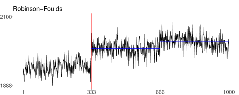
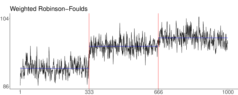
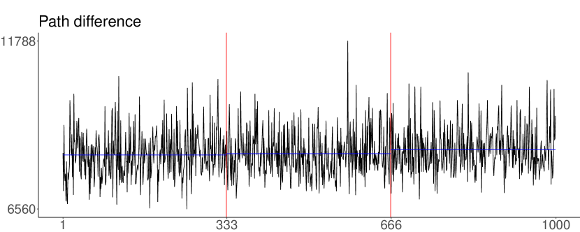
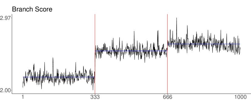
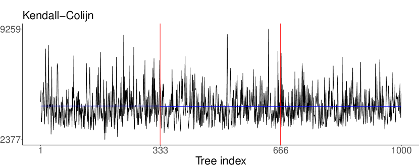
Figure 1: Topology trace plots for the Ebola analysis using five different phylogenetic distance metrics. The X-axis shows the index of the sampled tree (thinned sample), while the Y-axis shows the phylogenetic distance from the first tree. Red vertical lines denote iteration 333 and 666. Note how certain distance metrics show clear jumps between the separate runs, while for others the traces seem totally homogeneous.

Figure 1 shows the topology trace plots for the MCMC sample using five different phylogenetic distance metrics. What is immediately apparent from the thinned trace plot is the fact that, using certain distance metrics, the posterior sample of trees seems to be divided into three distinct parts at iterations 333 and 666. This suggests that three independent replicate analyses were combined to obtain a posterior samples of trees in the study of Dudas et al. (2017), which has been confirmed by the respective authors. Bayesian phylogenetic inference on large data sets indeed commonly employs the practice of concatenating the samples of several independent chains to both reduce computation time (by increasing the ESS values of continuous parameters) and assess convergence towards the same posterior. Three of the topology trace plots in Figure 1 therefore suggest a discrepancy between the posterior space explored by the three chains. Whether this indicates failure to converge to the same posterior, a case of extremely slow / poor mixing, or something else entirely is not clear. Intriguingly, this behaviour is not detected at all using certain other metrics, more specifically the path difference and Kendall-Colijn distance (with $\lambda$=0).

Subsample	1-1000	1-333	334-666	667-1000
Estimator (RF)
Approximate ESS	362	181	150	143
Split frequency ESS	446	279	273	276
Fréchet correlation ESS	83	229	209	211
Median pseudo-ESS	44	333	334	333
Minimum pseudo-ESS	15	276	285	271
MDS ESS	2	7	3	5
Estimator (wRF)
Approximate ESS	864	299	292	296
Split frequency ESS	446	279	273	276
Fréchet correlation ESS	46	238	189	212
Median pseudo-ESS	12	282	280	282
Minimum pseudo-ESS	3	189	189	177
MDS ESS	2	20	8	6
Estimator (PD)
Approximate ESS	1000	333	334	333
Split frequency ESS	446	279	273	276
Fréchet correlation ESS	280	292	279	299
Median pseudo-ESS	1000	333	334	333
Minimum pseudo-ESS	631	205	166	239
MDS ESS	1000	333	334	333
Estimator (BS)
Approximate ESS	710	290	278	287
Split frequency ESS	446	279	273	276
Fréchet correlation ESS	22	222	139	189
Median pseudo-ESS	4	261	230	256
Minimum pseudo-ESS	2	187	108	89
MDS ESS	2	88	12	6
Estimator (KC)
Approximate ESS	1000	333	334	333
Split frequency ESS	446	302	296	226
Fréchet correlation ESS	593	279	273	275
Median pseudo-ESS	1000	333	334	333
Minimum pseudo-ESS	518	261	148	181
MDS ESS	861	333	280	272

Table 1: ESS estimates from the treess package for the full sample and the three sub-samples. Values below the often used (although somewhat arbitrary) threshold of 200 are made bold. The phylogenetic distance metrics are here labeled using the following codes: RF = Robinson-Foulds, wRF = weighted Robinson-Foulds, PD = Path Difference, BS = Branch Score, KC = Kendall-Colijn. Like the topology trace plots, ESS’s computed using KC or PD do not show the same discrepancies as ESS’s computed using other metrics. The different estimators also do not all behave in the same way.

Applying the standard treess procedure for the different topological ESS estimators and using the different phylogenetic distance metrics produces a wide range of results which are listed in table 1. The ESS of the complete sample is not always greater than the sum of the ESS’s of the subsamples, which can be expected if the subsamples explore differents parts of tree space. Another distinction similar to the one in the topology trace plots can be noted: the path difference and Kendall-Colijn distance do not seem to pick up the same patterns as the other metrics, and generally seem overly optimistic about mixing based on the ESS values.

4 ESS values of individual tree splits

The approach by Guimarães Fabreti and Höhna (2021) does not aim to compute an ESS for the entire topology. Instead, each split in the tree is considered individually as a binary parameter (1=present, 0=absent) for which an ESS is computed using standard methodology. Figure 2 shows the cumulative density of ESS values of the $6859$ splits observed in trees generated by the MCMC algorithm. The vast majority of these (94%) have an ESS above the often used cutoff value of $200$. Almost half (46%) have an ESS of 1000, equal to the actual sample size. Although not pictured here, the three subsamples showed a nearly identically shaped distribution of individual split ESS’s. From this perspective, the mixing in topological space is quite optimistic.

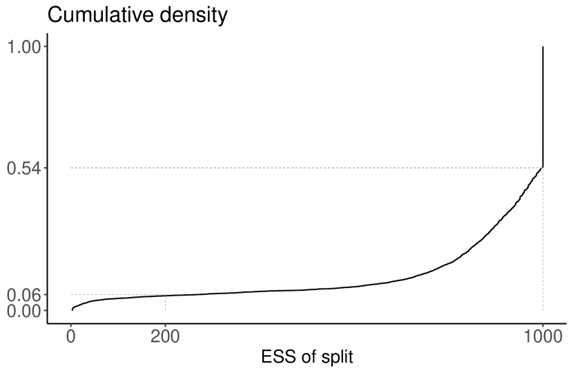
Figure 2: Cumulative density of ESS’s of individual splits in the sampled trees. ESS values 200 and 1000 are indicated and connected to their corresponding cumulative density values with dotted lines. Less than 6% of the splits have an ESS below the often used threshold of 200, suggesting satisfactory convergence in topological space. These ESS values were computed using the convenience R package.

5 Trace plots and ESS values of continuous parameters and tree statistics

Figure 3 shows trace graphs of the age of the root node and the tree length. The height of the root - a continuous parameter often evaluated using standard methodology - shows a well mixed chain with a satisfactory ESS. The trace of the tree length, which is more rarely assessed as it is not typically a statistic of interest, shows three somewhat distinguishable subsamples, as well as a very poor ESS. This is more in-line with the topological diagnostics.

Figure 3: Trace plots for the root node height (”Tree height”) and tree length (”Tree length”). Tree length refers to the sum of all tree branches, and is thus a statistic closely related to the topology of the tree. The root height, a commonly evaluated parameter, shows satisfactory mixing, while the tree length, which is rarely evaluated, shows poor mixing.

6 MCC trees

The observed discrepancies in the explored posterior topological space seen in the sample raises the question of what these differences actually reflect in terms of phylogenetic inference. In order to obtain some insights into this, we can compare the topology of the Maximum-Clade-Credibility (MCC) trees between the three subsamples.

Figure 4 shows a tanglegram comparing the MCC trees of the three subsamples and the entire sample by linking the corresponding taxa to each other. Taxa are coloured by country of origin. The figure also contains the MCC tree of samples 334 - 1000.The ESS values generated by tracer when only considering the last two subsections are also noticeably better than for the full sample: 547 and 272 for root height and tree length respectively. The trees all have the same overall shape, but several clades end up in different locations depending on the subsample. An obvious example of this is the clade of taxa largely sampled in Guinea with relatively recent sampling dates that switched branches with a closely clustered clade of Sierra-Leone based taxa. There also appears to be substantial uncertainty about the locations of nodes near the root of the tree.

Figure 4: Tanglegram of the MCC trees of the three subsamples, the combination of subsamples 2 and 3, and the whole sample. The tips of the trees are connected to each other by lines, coloured by the country of origin. Disagreement between the subsamples regarding the location of several clades is apparent by the fact that the lines connecting the tips of these clades are not parallel.

7 Approximate SPR distances

Another commonly used phylogenetic distance metric is the subtree prune-and-regraft (SPR) distance. This metric is often preferred by phylogeneticists because it reflects the minimum number of SPR operations required to go from one tree to another, which is more interpretable than other distance metrics. These and similar operations are often used to search phylogenetic tree space.

Calculation of SPR distances is computationally intensive for large trees such as the Ebola trees considered in this paper. In our case, calculation of a single SPR distance could last anywhere from 10 minutes to more than a day. This is substantially longer than any other metric discussed in the paper, and makes it unusable for our purposes. Therefore, we used the approximate SPR distances (aSPR) instead ( de Oliveira Martins et al. (2008)), whose computation time - similarly to the five other distance metrics - was in the seconds. Figure 5 shows a heat map of all the pairwise aSPR distances between sampled trees. Distances above 1300 are coloured grey. The three sections of the combined sample can be clearly distinguished by the block structure, as the distances between them tend to be substantially larger than the differences within them, corroborating the findings in figure 1. The differences between the three chains in terms of SPR moves are substantial and indicate that they in fact explore different modes in the posterior distribution of trees.

Figure 5: Pairwise approximate SPR (aSPR) distances between trees. Distances above 1300 are coloured grey. Discrepancies between the three subsamples are particularly pronounced, as the number of aSPR moves between trees is substantially larger between the subsamples than within them.

8 Conclusion

In this case study, we applied an ensemble of diagnostics in topological space on a set of large trees, obtained through Bayesian phylogenetic inference under a set of complex models and through combining the output of three independent replicate analyses. Importantly, we find that the different approaches to evaluating topological convergence can lead to drastically different conclusions, a finding that to the best of our understanding has not been observed to this extent before. It is likely that a combination of the complexity of the model, the size of the dataset, and the fact that we looked at samples that result from three different / independent analysis replicates – as opposed to only just one – allowed us to observe these phenomena that went unnoticed before. This finding stresses the importance of assessing topological convergence to the posterior and not merely continuous parameter and (joint) density convergence, which is the current benchmark in nearly all Bayesian phylogenetic and phylodynamic studies.

The various diagnostics we employed have revealed discrepancies between the posterior spaces explored by the MCMC algorithm that would typically have gone unnoticed using standard diagnostics for continuous parameters. Whether these discrepancies affect inferences on estimates of parameters of interest downstream in the analysis is not yet clear, and warrants further research. The impact of decisions such as which ESS estimator and topological distance metrics to use is not yet fully understood, and it is likely that these different approaches capture different aspects of convergence and mixing. SPR distances between the trees did suggest that the trees explored by the three subsamples differ in a topologically substantial way, which is line with the findings from the topological ESS estimators and the topology trace plots using (weighted) Robinson-Foulds distances and the branch score, as opposed to the other metrics we employed.

Graphing a topological trace plot using the (weighted) Robinson-Foulds distance or the branch score seemed to be the most informative approach for this data set, as these metrics were capable of discriminating between the three subsamples and suggested a discrepancy in terms of explored topological space. Analogously, the topological ESS’s estimators computed with those metrics tended to be more pessimistic - or realistic - about the information contained in the sample. These methods can rather easily implemented in existing software packages, which could improve current practice regarding convergence assessment of Bayesian phylogenetic and phylodynamic analyses.

Finally, our findings raise important questions as to how the output of replicate Bayesian phylogenetic and phylodynamic analyses should be combined when discrepancies in topological space are detected. These replicate analyses produce approximate samples from different regions of the posterior distribution. A key open question stemming from our work is how to combine these samples in such a way that preserves the mode structure, i.e., such that samples from higher modes are present in the combined sample more often than samples from the lower modes. Simply combining the samples with equal weights - which is currently standard practice - might not produce samples from the correct posterior, but techniques such as importance sampling could be employed to weight samples proportionally to their density.

9 Competing interests

No competing interest is declared.

10 Author contributions statement

M.B. and G.B. initialised the study. M.B. performed the analyses and wrote the manuscript. G.D. created the tanglegrams and computed the aSPR distances. L.M.C., J.G., F.A.M., A.R., M.A.S., G.D., S.L., P.L., and G.B. provided valuable guidance and feedback. All authors reviewed the manuscript.

11 Acknowledgments

The authors thank Andrew Magee for their valuable technical support. S.L.H. and G.B. acknowledge support from the Research Foundation - Flanders (“Fonds voor Wetenschappelijk Onderzoek - Vlaanderen,” G0E1420N). G.B. acknowledges support from the Internal Funds KU Leuven (Grant No. C14/18/094), from the Research Foundation - Flanders (“Fonds voor Wetenschappelijk Onderzoek - Vlaanderen,” G098321N) and from the European Union Horizon 2023 RIA project LEAPS (grant agreement no. 101094685). P.L., M.A.S. and A.R. acknowledge support from the Wellcome Trust (Collaborators Award 206298/Z/17/Z, ARTIC network), the European Research Council (grant agreement no. 725422 – ReservoirDOCS) and the National Institutes of Health (NIH) (R01 AI153044). F.A.M. and M.A.S. acknowledge further support from the NIH through R01 AI162611. P.L. acknowledges support from the Research Foundation, Flanders (“Fonds voor Wetenschappelijk Onderzoek - Vlaanderen,” G066215N, G0D5117N and G0B9317N) and from the European Union Horizon 2020 project MOOD (grant agreement no. 874850). M.B. and G.B. acknowledge support from the DURABLE EU4Health project 02/2023-01/2027, which is co-funded by the European Union (call EU4H-2021-PJ4) under Grant Agreement No. 101102733. Views and opinions expressed are however those of the author(s) only and do not necessarily reflect those of the European Union or the European Health and Digital Executive Agency. Neither the European Union nor the granting authority can be held responsible for them.

12 Supplementary Materials

Figure S1: Tanglegram of the MCC trees of the three subsamples, the latter two subsamples combined, and the whole sample. Nodes with posterior support $<$0.1 are collapsed. When collapsing the nodes with low posterior support ($<$10%), the differences in topology between the subsamples seem less pronounced. However, adding the first subsamples to the latter two (MCC tree ‘23’) strongly impacts the (structure of the) overall MCC tree (‘total’).

((a)) Subsample 1-333

((b)) Subsample 334-666

((c)) Subsample 667-1000

((d)) Subsample 334-1000

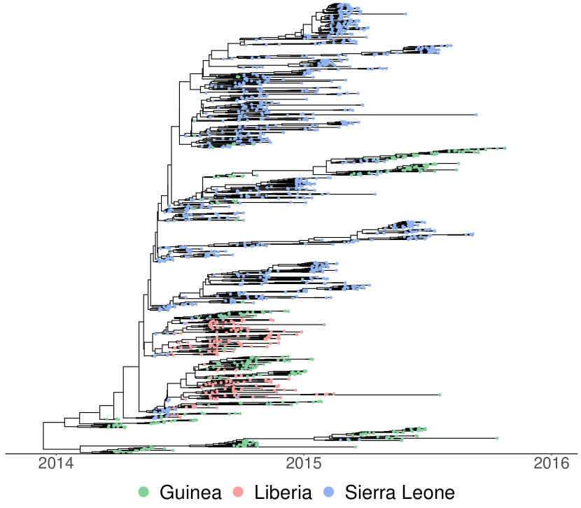
((e)) Total sample

Figure S2: MCC trees of the different subsamples with taxa coloured by origin country, analogous to the tanglegrams of Figures 4 and  S1.

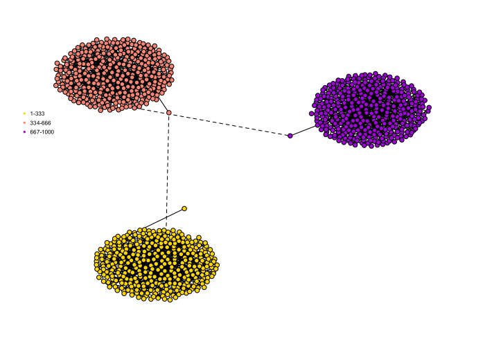
Figure S3: Network graph of approximate SPR (aSPR) distances between sampled trees. Each node represents a sampled tree and distances between nodes approximate the aSPR distance between the trees. Nodes are coloured by subsection of the sample. The edges correspond to trees that were subsequently sampled. This graph was generated using a force-directed layout based on the Fruchterman-Reingold algorithm, as implemented in the R package qgraph version 1.9.8. (Epskamp et al. [2023]). The exact location of the nodes has no real meaning, only their relative locations. As expected from the topological trace plots, the three subsamples are also distinctly recognisable in this network graph. Note that the first tree in each subsample is somewhat distinct from the rest of the trees in that subsample, potentially pointing to a somewhat too low burn-in while processing the sampled trees from the Bayesian phylogenetic analysis.

References

- Attwood et al. [2022] S. Attwood, S. Hill, D. Aanensen, T. Connor, and O. Pybus. Phylogenetic and phylodynamic approaches to understanding and combating the early sars-cov-2 pandemic. Nature Reviews Genetics, 23:1–16, 04 2022. 10.1038/s41576-022-00483-8.
- de Oliveira Martins et al. [2008] L. de Oliveira Martins, E. Leal, and H. Kishino. Phylogenetic detection of recombination with a Bayesian prior on the distance between trees. PloS one, 3(7):e2651–e2651, 2008.
- Dudas et al. [2017] G. Dudas, L. M. Carvalho, T. Bedford, A. J. Tatem, G. Baele, N. R. Faria, D. J. Park, J. T. Ladner, A. Arias, D. Asogun, F. Bielejec, S. L. Caddy, M. Cotten, J. D’Ambrozio, S. Dellicour, A. D. Caro, J. W. Diclaro, S. Duraffour, M. J. Elmore, L. S. Fakoli, O. Faye, M. L. Gilbert, S. M. Gevao, S. Gire, A. Gladden-Young, A. Gnirke, A. Goba, D. S. Grant, B. L. Haagmans, J. A. Hiscox, U. Jah, J. R. Kugelman, D. Liu, J. Lu, C. M. Malboeuf, S. Mate, D. A. Matthews, C. B. Matranga, L. W. Meredith, J. Qu, J. Quick, S. D. Pas, M. V. T. Phan, G. Pollakis, C. B. Reusken, M. Sanchez-Lockhart, S. F. Schaffner, J. S. Schieffelin, R. S. Sealfon, E. Simon-Loriere, S. L. Smits, K. Stoecker, L. Thorne, E. A. Tobin, M. A. Vandi, S. J. Watson, K. West, S. Whitmer, M. R. Wiley, S. M. Winnicki, S. Wohl, R. Wölfel, N. L. Yozwiak, K. G. Andersen, S. O. Blyden, F. Bolay, M. W. Carroll, B. Dahn, B. Diallo, P. Formenty, C. Fraser, G. F. Gao, R. F. Garry, I. Goodfellow, S. Günther, C. T. Happi, E. C. Holmes, B. Kargbo, S. Keïta, P. Kellam, M. P. G. Koopmans, J. H. Kuhn, N. J. Loman, N. Magassouba, D. Naidoo, S. T. Nichol, T. Nyenswah, G. Palacios, O. G. Pybus, P. C. Sabeti, A. Sall, U. Ströher, I. Wurie, M. A. Suchard, P. Lemey, and A. Rambaut. Virus genomes reveal factors that spread and sustained the Ebola epidemic. Nature, 544(7650):309–315, Apr 2017. 10.1038/nature22040. URL https://doi.org/10.1038%2Fnature22040.
- Epskamp et al. [2023] D. Epskamp, G. Costantini, J. Haslbeck, A. Isvoranu, A. Cramer, L. Waldorp, V. Schmittmann, and D. Borsboom. qgraph: Graph plotting methods, psychometric data visualization and graphical model estimation. CRAN repository, 2023.
- Gill et al. [2013] M. Gill, P. Lemey, N. Faria, A. Rambaut, B. Shapiro, and M. A. Suchard. Improving Bayesian population dynamics inference: A coalescent-based model for multiple loci. Molecular Biological Evolution, 30(3):713–724, 2013.
- Guimarães Fabreti and Höhna [2021] L. Guimarães Fabreti and S. Höhna. Convergence assessment for Bayesian phylogenetic analysis using MCMC simulation. Methods in Ecology and Evolution, 13(1):77–90, 2021.
- Kendall and Colijn [2016] M. Kendall and C. Colijn. Mapping phylogenetic trees to reveal distinct patterns of evolution. Molecular Biology and Evolution, 33(10):2735–2743, 2016.
- Kruskal [1964a] J. B. Kruskal. Multidimensional scaling by optimizing goodness of fit to a nonmetric hypothesis. Psychometrika, 29:1–27, 1964a.
- Kruskal [1964b] J. B. Kruskal. Nonmetric multidimensional scaling: A numerical method. Psychometrika, 29:115–129, 1964b.
- Kuhner and Felsenstein [1994] M. Kuhner and J. Felsenstein. A simulation comparison of phylogeny algorithms under equal and unequal evolutionary rates. Molecular Biology and Evolution, 11(3):459–468, 1994.
- Lanfear et al. [2016] R. Lanfear, X. Hua, and D. L. Warren. Estimating the effective sample size of tree topologies from Bayesian phylogenetic analyses. Genome Biology and Evolution, 8(8):2319–2332, 2016.
- Magee et al. [2023] A. Magee, M. Karcher, F. Matsen IV, and V. Minin. How trustworthy is your tree? Bayesian phylogenetic effective sample size through the lens of Monte Carlo error. Bayesian Analysis, 1(1):1–29, 2023.
- Martin [2023] S. R. Martin. Treedist: Calculate and map distances between phylogenetic trees. 2023.
- Plummer et al. [2020] M. Plummer, N. Best, K. Cowles, K. Vines, D. Sarkay, D. Bates, R. Almond, and A. Magnusson. Package ’coda’. CRAN, 2020.
- R-team [2022] R-team. R: A language and environment for statistical computing. 2022.
- Rambaut et al. [2018] A. Rambaut, A. Drummond, D. Xie, G. Baele, and M. Suchard. Posterior summarisation in Bayesian phylogenetics using Tracer 1.7 (available at http://beast.community/tracer). Systematic Biology, 67(5):901–904, 2018.
- Robinson and Foulds [1979] D. Robinson and L. Foulds. Comparison of weighted labelled trees. In: Horadam, A.F., Wallis, W.D. (eds) Combinatorial Mathematics VI, 748:119–126, 1979.
- Robinson and Foulds [1981] D. Robinson and L. Foulds. Comparison of phylogenetic trees. Mathematical Biosciences, 53(1-2):131–147, 1981.
- Schliep et al. [2022] K. Schliep, E. Paradis, L. de Oliveira Martins, A. Potts, and T. White. Package ’phangorn’. CRAN, 2022.
- Steel and Penny [1993] M. A. Steel and D. Penny. Distributions of tree comparison metrics - some new results. Syst Biol., 42:126–141, 1993.
- Suchard et al. [2018] M. A. Suchard, P. Lemey, G. Baele, A. J. Drummond, and A. Rambaut. Bayesian phylogenetic and phylodynamic data integration using BEAST 1.10. Virus Evolution, 4(1):vey016, 2018.
- Whidden et al. [2013] C. Whidden, R. Beiko, and N. Zeh. Fixed-parameter algorithms for maximum agreement forests. SIAM Journal on Computing, 42(4):1431–1466, 2013.
- Wirth and Duchene [2022] W. Wirth and S. Duchene. Real-Time and Remote MCMC Trace Inspection with Beastiary. Molecular Biology and Evolution, 39(5):msac095, 05 2022. ISSN 1537-1719. 10.1093/molbev/msac095. URL https://doi.org/10.1093/molbev/msac095.
- Xu et al. [2022] S. Xu, L. Li, X. Luo, M. Chen, W. Tang, L. Zhan, Z. Dai, T. Lam, Y. Guan, and G. Yu. Ggtree: A serialized data object for visualization of a phylogenetic tree and annotation data. iMeta, 1(e56), 2022.