Doubly Robust Inference in Causal Latent Factor Models
00footnotetext: Abadie: abadie@mit.edu. Agarwal: aa5194@columbia.edu. Dwivedi: dwivedi@cornell.edu. Shah: abhin@mit.edu.| Alberto Abadie | Anish Agarwal | |
| MIT | Columbia | |
| Raaz Dwivedi | Abhin Shah | |
| Cornell Tech | MIT |
March 5, 2024
Abstract
This article introduces a new framework for estimating average treatment effects under unobserved confounding in modern data-rich environments featuring large numbers of units and outcomes. The proposed estimator is doubly robust, combining outcome imputation, inverse probability weighting, and a novel cross-fitting procedure for matrix completion. We derive finite-sample and asymptotic guarantees, and show that the error of the new estimator converges to a mean-zero Gaussian distribution at a parametric rate. Simulation results demonstrate the practical relevance of the formal properties of the estimators analyzed in this article.
1 Introduction
This article presents a novel framework for the estimation of average treatment effects in modern data-rich environments in the presence of unobserved confounding. Modern data-rich environments are characterized by repeated measurements of outcomes, such as clinical metrics or purchase history, across a substantial number of units—be it patients in medical contexts or customers in online retail. As an example, consider an internet-retail platform where customers interact with various product categories. For each consumer-category pair, the platform makes decisions to either offer a discount or not, and records whether the consumer purchased a product in the category. Given an observational dataset capturing such interactions, our objective is to infer the causal effect of offering the discount on consumer purchase behavior. More specifically, we aim to infer two kinds of treatment effects: tailored to product categories, the average impact of the discount on a product across consumers, and tailored to consumers, the average impact of the discount on a consumer across product categories. This task is challenging due to unobserved confounding that may cause spurious associations between discount allocation and product purchase.
There are two widely used approaches for treatment effect estimation: outcome-based methods and assignment-based methods. Outcome-based methods operate by imputing the missing potential outcomes for each consumer-product category pair. This process involves predicting whether a consumer, who received a discount, would have made the purchase without the discount (i.e., the potential outcome without discount), and conversely, if a consumer who did not receive the discount would have purchased the product had they received the discount (i.e., the potential outcome with discount). Assignment-based methods predict the probability with which a consumer is offered the discount on a product category, and inversely weight the observed outcomes by these estimated probabilities.
A substantial and influential body of literature has explored outcome-based methods, particularly in settings where all confounding factors are measured (see, e.g., Cochran,, 1968; Rosenbaum and Rubin,, 1983; Angrist,, 1998; Abadie and Imbens,, 2006, among many others). Imputing potential outcomes in the presence of unobserved confounders poses a more complex challenge, and the existing literature devoted to this problem is relatively small. In this context, a commonly adopted framework is the latent factor framework (Bai and Ng,, 2002; Bai,, 2009), wherein each element of the large-dimensional outcome vector is influenced by the same low-dimensional vector of unobserved confounders. A closely related approach is the technique of matrix completion (see, e.g., Chatterjee,, 2015; Athey et al.,, 2021; Bai and Ng,, 2021; Agarwal et al., 2023a, ; Dwivedi et al., 2022a, ) which has found widespread applications in recommendation systems and panel data models.
In this article, we propose a doubly-robust estimator (see Bang and Robins,, 2005; Chernozhukov et al.,, 2018) of average treatment effects in the presence of unobserved confounding. This estimator leverages information on both the outcome process and the treatment assignment mechanism under a latent factor framework. It combines outcome imputation and inverse probability weighting with a new cross-fitting approach for matrix completion. We show that the proposed doubly-robust estimator has better finite-sample guarantees than alternative outcome-based and assignment-based estimators. Furthermore, the doubly-robust estimator is approximately Gaussian, asymptotically unbiased, and converges at a parametric rate, under provably valid error rates for matrix completion, irrespective of other properties of the matrix completion algorithm used for estimation, making it relatively agnostic to the specific matrix completion used.
Terminology and notation. For any real number , is the greatest integer less than or equal to . For any positive integer , denotes the set of integers from to , i.e., . We use to denote any generic universal constant, whose value may change between instances. For any , and . For any two deterministic sequences and where is positive, means that there exist a finite and a finite such that for all . Similarly, means that for every , there exists a finite such that for all . For a sequence of random variables and a sequence of positive constants , means that the sequence is stochastically bounded, i.e., for every , there exists a finite and a finite such that for all . Similarly, means that the sequence converges to zero in probability, i.e., for every and , there exists a finite such that for all .
A mean-zero random variable is subGaussian if there exists some such that for all . Then, the subGaussian norm of is given by . A mean-zero random variable is subExponential if there exist some such that for all . Then, the subExponential norm of is given by . Let denote the uniform distribution over the interval for such that . Let denote the Gaussian distribution with mean and variance .
For a vector , we denote its coordinate by and its -norm . For a matrix , we denote the element in row and column by , the row by , the column by , the largest eigenvalue by , and the smallest by . Given a set of indices and , is a sub-matrix of corresponding to the entries in . Further, we denote the Frobenius norm by , the norm by , the norm by , and the maximum norm by . Given two matrices , the operators and denote element-wise multiplication and division, respectively, i.e., when , and when . When is a binary matrix, i.e., , the operator is defined such that if and if for . Given two matrices and , the operator denotes the Khatri-Rao product (or column-wise product) of and , i.e., such that where . For random objects and , means that is independent of .
2 Setup
Consider a setting with units and measurements per unit. For each unit-measurement pair , we observe a treatment assignment and the value of the outcome under the treatment assignment. For the ease of exposition, we focus on binary treatments. However, our framework can be easily generalized to multi-ary treatments.
We operate within the Neyman-Rubin potential outcomes framework and denote the potential outcome for unit and measurement under treatment by . Here, it is implicitly assumed that the potential outcome for any unit and measurement does not depend on the treatment assignment for any other unit-measurement pair, i.e., there are no spillover effects across units or measurements. In the context of online retail data, the assumption of no spillovers across measurements is justified if the cross-elasticity of demand across product categories, , is low. The observed outcomes depend on the potential outcomes and the treatment assignments,
| (1) |
for all .
2.1 Sources of stochastic variation
In the setup of this article, each unit is characterized by a set of unknown parameters, , which we treat as fixed. Potential outcomes and treatment assignments are generated as follows: for all , and ,
| (2) | |||
| and | |||
| (3) | |||
where and are mean-zero random variables, and
| (4) |
It follows that is the mean of the potential outcome , and is the unknown assignment probability or latent propensity score. The matrices , , and collect all mean potential outcomes and assignment probabilities. Then, the matrices , and capture all sources of randomness in potential outcomes and treatment assignments.
Our setup allows to be arbitrarily associated with , inducing unobserved confounding. The identification restrictions made in Section 4 imply that , and include all confounding factors, and require .
2.2 Target causal estimand
For any given measurement , we aim to estimate the effect of the treatment averaged over all units,
| (5) | |||
| where | |||
| (6) | |||
It is straightforward to adapt the methods in this article to the estimation of alternative parameters, like the average treatment effect across measurements for each unit , or the estimation of treatment effects over a subset of the units, .
3 Estimation
In this section, we propose an estimator that uses the treatment assignment matrix and the observed outcomes matrix to estimate the target causal estimand , where
| (7) |
Our estimator leverages matrix completion as a key subroutine. We start with a brief overview of matrix completion below.
3.1 Matrix completion: A primer
Consider a matrix of parameters . While is unobserved, we observe the matrix where denotes a missing value. The relationship between and is given by
| (8) |
where represents a matrix of noise, is a masking matrix, and the operator is as defined in Section 1. A matrix completion algorithm, denoted by MC, takes the matrix as its input, and returns an estimate for the matrix , which we denote by or . In other words, MC produces an estimate of a matrix from noisy observations of a subset of all the elements of the matrix.
The matrix completion literature is rich with algorithms MC that provide error guarantees, namely bounds on for a suitably chosen norm/metric , under a variety of assumptions on the triplet . Typical assumptions are is low-rank, the entries of are independent, mean-zero and sub-Gaussian random variables, and the entries of are independent Bernoulli random variables. Though matrix completion is commonly associated with the imputation of missing values, a typically underappreciated aspect is that it also denoises the observed matrix. Even when each entry of is observed, subtracts the effects of from , i.e., it performs matrix denoising. Refer to Nguyen et al., (2019) for a survey of various matrix completion algorithms.
 |
 |
 |
 |
3.2 Key building blocks
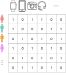
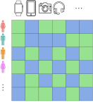
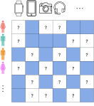
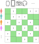
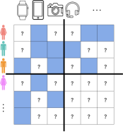
We now define and express matrices that are related to the quantities of interest , and in a form similar to Eq. 8. See Figure 1 for a visual depiction of these matrices.
-
•
Outcomes: Let be a matrix with -th entry equal to if and equal to , otherwise. Here, is the matrix with all entries equal to one. Analogously, let be a matrix with -th entry equal to if and equal to , otherwise. In other words, and capture the observed components of and , respectively, with missing entries denoted by . Then, we can write
(9) -
•
Treatments: From Eq. 3, we can write
(10)
as all the entries in are observed. Building on the earlier discussion, the application of matrix completion yields the following estimates:
| (11) |
where the algorithm MC may vary for , , and . Because all entries of are observed, denoises but does not need to impute missing entries. From Eq. 9 and Eq. 11, it follows that and depend on and , whereas depends only on .
In this section, we deliberately leave the matrix completion algorithm MC as a “black-box”. In Section 4, we establish finite-sample and asymptotic guarantees for our proposed estimator, contingent on specific properties for MC. In Section 5, we propose a novel end-to-end matrix completion algorithm that satifies these properties.
Given matrix completion estimates of , we formulate two preliminary estimators for : an outcome imputation estimator, which uses and only, and an inverse probability weighting estimator, which uses only. Then, we combine these to obtain a doubly robust estimator of .
Outcome imputation (OI) estimator. Let denote the -th entry of for , and . The OI estimator for is defined as follows:
| (12) | |||
| where | |||
| (13) | |||
That is, the OI estimator is obtained by taking the difference of the average value of the -th column of the estimates and . The quality of the OI estimator depends on how well and approximate the mean potential outcome matrices and , respectively.
Inverse probability weighting (IPW) estimator. Let denote the -th entry of for and . The IPW estimate for is defined as follows:
| (14) | |||
| where | |||
| (15) | |||
That is, the IPW estimator is obtained by taking the difference of the average value of the -th column of the matrices and , replacing unobserved entries with zeros, and weighting each outcome by the inverse of the estimated assignment probability to account for confounding. The quality of the IPW estimate depends on how well approximates the probability matrix .
The matrix completion-based OI and IPW estimators in Eq. 12 and Eq. 14 have the same form as the classical OI and IPW estimators, which are derived for settings where all confounders are observed (e.g., Imbens and Rubin,, 2015). In contrast to the classical setting, our framework is one with unmeasured confounding.
3.3 Doubly robust (DR) estimator
The DR estimate for combines the estimates , and from Eq. 11. It is defined as follows:
| (16) | |||
| where | |||
| (17) | |||
| and | |||
| (18) | |||
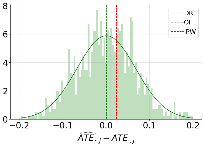
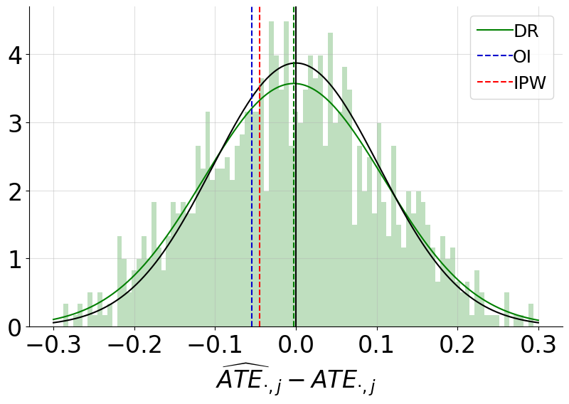
In Section 4, we prove that consistently estimates as long as either is consistent for or is consistent for , i.e., it is doubly robust. Furthermore, we show that the DR estimator provides superior finite sample guarantees than the OI and IPW estimators, and that it satisfies a central limit theorem at a parametric rate under weak conditions on the convergence rate of the matrix completion routine. Using simulated data, Figure 2 demonstrates the improved performance of DR, relative to OI and IPW. Despite substantial biases observed in both OI and IPW estimates, the error of the DR estimate demonstrates a mean-zero Gaussian distribution. We provide a detailed description of the simulation setup in Section 6.
 |
4 Main Results
This section presents the formal results of the article. Section 4.1 details assumptions, Section 4.2 discusses finite-sample guarantees, and Section 4.3 presents a central limit theorem for .
4.1 Assumptions
Requirements on data generating process. We make two assumptions on how the data is generated. First, we impose a positivity condition on the assignment probabilities.
Assumption 1 (Positivity).
The unknown assignment probability matrix is such that
| (19) |
for all and , where is a constant.
1 requires that the propensity score for each unit-outcome pair is bounded away from and , implying that any unit-item pair can be assigned either of the two treatments. An analogous assumption is pervasive in causal inference models that assume observed confounding. For simplicity of exposition and to avoid notational clutter, 1 requires Eq. 19 for all outcomes, . However, it is only necessary that Eq. 19 holds for the outcomes of interest, , for which is estimated. Our framework leverages the availability of a large number of outcomes to control for the confounding effect of latent variables. In practical applications, however, may be estimated for a select group of those outcomes. For example, in synthetic control settings (Abadie et al.,, 2010), is estimated only for post-treatment outcomes. In that case, the positivity assumption applies only for the selected subset of outcomes for which is estimated.
Next, we formalize the requirements on the noise variables.
Assumption 2 (Zero-mean, independent, and subGaussian noise).
.
-
(a)
have zero mean entries,
-
(b)
,
-
(c)
All entries of are mutually independent,
-
(d)
are mutually independent (across ) for every , and
-
(e)
Each entry of and has subGaussian norm bounded by a constant .
2(a) defines as the means of the potential outcomes and treatment assignment in Eqs. 2 and 3. 2(b) implies that capture all confounding factors. 2(c) imposes independence across units and measurements in the noise . 2(d) imposes independence across units in the noise , for every measurement. Finally, 2(e) is mild and useful to derive finite-sample guarantees. For the central limit theorem in Section 4.3, subGaussianity could be disposed of by restricting the moments of and . Note that 2 does not restrict the dependence between and .
Requirements on matrix completion estimators. First, we assume the estimate is consistent with 1.
Assumption 3.
The estimated probability matrix is such that
| (20) |
for all and , where .
3 is achieved by truncating entries of to the range . Second, our theoretical analysis requires independence between certain sub-matrices of the estimates from Eq. 11, and the noise matrices . We formally state this independence condition as an assumption below.
 |
Assumption 4.
There exists partitions of the units in and of the measurements , such that each unit is assigned to or with equal probability, each measurement is assigned to or with equal probability, and for each block ,
| (21) | |||
| and | |||
| (22) | |||
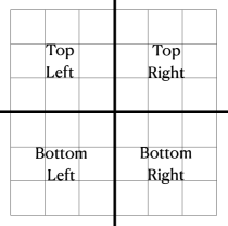
Without loss of generality, suppose and . Figure 3 provides a schematic of the corresponding block partition . Eq. 21 requires that within each of the four blocks in , mean potential outcomes estimators and the assignment probability estimators are independent of the sub-matrix of for the same block. 2(b) implies that Eq. 22 holds provided is a function of only, as is the case for the matrix completion procedure in Eq. 11. Analogous conditions appear in the literature on doubly robust estimation under observed confounding (e.g., Definition 3.1 in Chernozhukov et al.,, 2018). Specifically, in that context, Chernozhukov et al., (2018) split the available data into -folds, and require estimates of propensities and outcomes in each fold to be independent of the noise in that fold. Section 5 provides a way to ensure 4 holds for any MC algorithm using a cross-fitting procedure as long as 2 holds.
Matrix completion error rates. The formal guarantees in this section depend on the normalized norms of the errors in estimating the unknown parameters . We use the following notation for these errors:
| (23) | |||
| where | |||
| (24) | |||
A variety of matrix completion algorithms deliver and , where . Throughout, our notation primarily tracks dependence on . We say that these normalized errors achieve the parametric rate when they have the same rate as . Section 5 explicitly characterizes and under low-rank assumptions on and for a particular matrix completion algorithm.
4.2 Non-asymptotic guarantees
The first main result of this section provides both a non-asymptotic error bound and an asymptotic consistency result for in terms of the errors and in Eq. 23.
Theorem 1 (Finite Sample Guarantees for DR).
The proof of Theorem 1 is given in Appendix B. Eqs. 25 and 26 bound the absolute error of the DR estimator by the rate of . When is lower bounded at the parametric rate of , has the same rate as .
Doubly robust behavior of . The error rate of immediately reveals that the DR estimate is doubly robust with respect to the error in estimating the mean potential outcomes and the assignment probabilities . First, the error decays at a parametric rate of as long as the product of error rates, , decays as . As a result, can exhibit a parametric error rate even when neither the mean potential outcomes nor the assignment probabilities are estimated at a parametric rate. Second, decays to zero as long as either of or decays to . Hence, is consistent as long as either the mean potential outcomes or the assignment probabilities are estimated consistently.
We next compare the performance of DR estimator with the OI and IPW estimators from Eqs. 12 and 14, respectively. Towards this goal, we characterize the estimation error of in terms of and of in terms of .
Proposition 1 (Finite Sample Guarantees for OI and IPW).
The proofs of Eq. 28 and Eq. 29 are given in Appendices D and E, respectively. Proposition 1 implies that in an asymptotic sequence with bounded , OI and IPW attain the parametric rate provided and are , respectively. The next corollary compares these error rates with those obtained for the DR estimator in Theorem 1.
Corollary 1 (Gains of DR over OI and IPW).
Corollary 1 demonstrates that the DR estimate’s error decay rate is consistently superior to that of the OI and IPW estimates across a variety of regimes for . Specifically, the error scales strictly faster than both and if the estimation errors of , , and converge slower than at the parametric rate . When the estimation errors of , , and all decay at a parametric rate, OI, IPW, and DR estimation errors decay also at a parametric rate.
4.3 Gaussian approximation
The next theorem, proven in Appendix C, establishes a Gaussian approximation for under mild conditions on error rates and .
Theorem 2 (Asymptotic Normality for DR).
Theorem 2 describes two simple requirements on the estimated and , under which exhibits an asymptotic Gaussian distribution centered at . Condition (C1) requires that the estimation errors of and converge to zero in probability. Condition (C2) requires that the product of the errors decays sufficiently fast, at a rate , ensuring that the bias of the normalized estimator in Eq. 34 converges to zero. Condition (C2) is similar to conditions in the literature on doubly-robust estimation of average treatment effects under observed confounding (e.g., Assumption 5.1 in Chernozhukov et al.,, 2018). Specifically, in that context, Chernozhukov et al., (2018) assume that the product of propensity estimation error and outcome regression error decays faster than .
Black-box asymptotic normality. We emphasize Theorem 2 applies to any matrix completion algorithm MC as long as conditions (C1) and (C2) are satisfied This property arises because the bias is dominated by the product of and , which can be shown to be for a broad class of MC algorithms under mild assumptions on . On the other hand, achieving such black-box asymptotic normality results for OI or IPW estimates is challenging, as their bias scales with individual error rates and , respectively, which are typically lower bounded at the parametric rate of . Our simulations in Section 6 corroborate these theoretical findings.
5 Matrix Completion with Cross-Fitting
In this section, we introduce a novel algorithm designed to construct estimators that adhere to 4 and satisfy conditions (C1) and (C2) in Theorem 2. We first explain why traditional matrix completion algorithms fail to deliver the properties required by 4. We then present Cross-Fitted-MC, a meta-algorithm that takes any matrix completion algorithm and uses it to construct that satisfy 4. Finally, we describe Cross-Fitted-SVD, an end-to-end algorithm obtained by combining Cross-Fitted-MC with the singular value decomposition (SVD)-based algorithm of Bai and Ng, (2021), and establish that it also satisfies conditions (C1) and (C2) in Theorem 2.
Traditional matrix completion. Estimators obtained from existing matrix completion algorithms need not satisfy 4. In particular, using the entire assignment matrix to estimate each element of typically results in a violation of in Eq. 21, as each entry of is allowed to depend on the entire noise matrix . For example, in spectral methods (e.g., Nguyen et al.,, 2019), is a function of the SVD of the entire matrix , and
| (35) |
for all in general, which implies that for every , . Similarly, in matching methods such as nearest neighbors (Li et al.,, 2019), is a function of the matches/neighbors estimated from the entire matrix . Dependence structures such as for any —which is weaker than Eq. 35—are enough to violate the requirement in Eq. 21.
Likewise, the requirement in Eq. 21 can be violated, because and depend respectively on and , which themselves depend on the entire matrix .
5.1 Cross-Fitted-MC: A meta-cross-fitting algorithm for matrix completion
We now introduce Cross-Fitted-MC, a cross-fitting approach that modifies any MC algorithm to produce that satisfy 4. Recall the setup from Section 3.1: Given an observation matrix , a matrix completion algorithm MC produces an estimate of a matrix of interest , where and are related via Eq. 8. With this background, we now describe the Cross-Fitted-MC meta-algorithm.
-
1.
The inputs are a matrix completion algorithm MC, an observation matrix , and a block partition of the set into four blocks as in 4.
-
2.
For each block , construct by applying MC on where denotes a masking matrix with -th entry equal to if and otherwise, and the operator is as defined in Section 1. In other words,
(36) -
3.
Return obtained by collecting together , with each entry in its original position.
We represent this meta-algorithm succinctly as below:
| (37) |
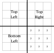
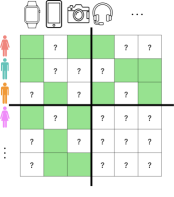
In summary, Cross-Fitted-MC produces an estimator such that for each block , the sub-matrix is constructed only using the entries of corresponding to the remaining three blocks of . See Figure 4 for a visualization of . The following result, proven in Section F.1, establishes generated by Cross-Fitted-MC satisfy 4.
Proposition 2 (Guarantees for Cross-Fitted-MC).
A host of MC algorithms are designed to de-noise and impute missing entries of matrices under random patterns of missingness; the most common missingness pattern studied is where each entry has the same probability of being missing, independent of everything else. In contrast, Cross-Fitted-MC generates patterns where all entries in one block are deterministically missing, as in Figure 4. A recent strand of research on the interplay between matrix completion methods and causal inference models—specifically, within the synthetic controls framework—has contributed matrix completion algorithms that allow for block missingness (see, e.g., Athey et al.,, 2021; Agarwal et al.,, 2021; Bai and Ng,, 2021; Agarwal et al., 2023b, ; Arkhangelsky et al.,, 2021; Agarwal et al., 2023a, ; Dwivedi et al., 2022a, ; Dwivedi et al., 2022b, ). However, it is a challenge to apply known theoretical guarantees for these methods to the setting in this article because of: (i) the use of cross-fitting—which creates blocks where all observations are missing—and (ii) outside of the completely-missing blocks, there can still be missing observations with heterogeneous probabilities of missingness. In the next section, we show how to modify any MC algorithm designed for block missingness patterns so that it can be applied to our setting with cross-fitting and heterogeneous probabilities of missingness outside the folds. For concreteness, we work with the Tall-Wide matrix completion algorithm of Bai and Ng, (2021).
 |
5.2 The Cross-Fitted-SVD algorithm
Cross-Fitted-SVD is an end-to-end MC algorithm obtained by instantiating the Cross-Fitted-MC meta-algorithm with the Tall-Wide algorithm of Bai and Ng, (2021), which we denote as TW. For completeness, we detail the TW algorithm in Section 5.2.1, and then use it to describe Cross-Fitted-SVD in Section 5.2.2.
5.2.1 The TW algorithm of Bai and Ng, (2021).
Bai and Ng, (2021) propose TW to impute missing values in those matrices where there exists a set of rows and a set of columns without missing entries. More concretely, for any matrix , let and denote the set of rows and columns, respectively, with all entries observed. Then, the block , where and , is such that all the missing entries in are a subset of it.
Given a rank hyper-parameter , produces an estimate of as follows:
-
1.
Run SVD separately on and , i.e.,
(41) and (42) where and . The columns of and are the left singular vectors of and , respectively, and the columns of and are the right singular vectors of and , respectively. The diagonal entries of and are the singular values of and , respectively, and the off-diagonal entries are zeros. This step of TW requires the existence of the fully observed blocks and , i.e., and cannot be empty.
-
2.
Let be the sub-matrix of that keeps the columns corresponding to the largest singular values only. Let be the sub-matrix of that keeps the columns corresponding to the largest singular values only and the rows corresponding to the indices in only. Obtain a rotation matrix as follows:
(43) That is, is obtained by regressing on . In essence, aligns the right singular vectors of and using the entries that are common between these two matrices, i.e., the entries corresponding to indices . The formal guarantees of the TW algorithm remains unchanged if one alternatively regresses on , or uses the left singular vectors of and for alignment.
-
3.
Let be the sub-matrix of that keeps the columns corresponding to the largest singular values only. Let be the sub-matrix of that keeps the columns corresponding to the largest singular values only. Return as an estimate for .
5.2.2 Cross-Fitted-SVD algorithm.
-
1.
The inputs are , for , and hyper-parameters , , , and such that and .
-
2.
Choose a random partition of and of such that each is assigned to or with equal probability and each is assigned to or with equal probability. Construct the block partition .
-
3.
Return where projects each entry of its input to the interval .
-
4.
Define as equal to , but with all missing entries in set to zero. Define analogously with respect to .
-
5.
Return .
-
6.
Return .
We provide intuition on the key steps of the Cross-Fitted-SVD algorithm next.
 |
 |
 |
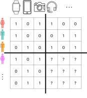
Computing . The estimate comes from applying Cross-Fitted-MC with TW on and truncating the entries of the resulting matrix to the range , in accordance with 3. The TW sub-routine is directly applicable to , because for any block the masked matrix has fully observed rows and fully observed columns. See Figure 5 for a visualization of .
Computing and . The estimates and are constructed by applying Cross-Fitted-MC with TW on and , which do not have missing entries. TW is not directly applicable on and , as both matrices may not have any rows and columns that are fully observed. See Figure 5 and Figure 5 for visualizations of and , respectively. However, notice that
| (44) | ||||
| and | ||||
| (45) | ||||
As a result, and provide estimates of and , respectively—recall the discussion in Section 3.1. To estimate and , we divide the entries of and by the entries of and , respectively. Adjustments of this type for heterogeneous missingness probabilities have been previously explored in Ma and Chen, (2019); Bhattacharya and Chatterjee, (2022).
5.3 Theoretical guarantees for Cross-Fitted-SVD
To establish theoretical guarantees for Cross-Fitted-SVD, we adopt three assumptions from Bai and Ng, (2021). The first assumption imposes a low-rank structure on the matrices , , and , namely that their entries are given by an inner product of latent factors.
Assumption 5 (Linear latent factor model on the confounders).
There exist constants and a collection of latent factors
| (46) |
such that the unobserved confounders satisfy the following factorization:
| (47) |
5 decomposes each of the unobserved confounders (, , and ) into low-dimensional unit-dependent latent factors (, , and ) and measurement-dependent latent factors (, , and ). In particular, every unit is associated with three low-dimensional factors: , , and . Similarly, every measurement is associated with three factors: , , and . Such low-rank assumptions are standard in the matrix completion literature.
The second assumption requires that the factors that determine , , and explain a sufficiently large amount of the variation in the data. This assumption is made on the factors of and instead of and as the TW algorithm is applied on and , instead of and (see steps 5 and 6 of Cross-Fitted-SVD). To determine the factors of and , let
| (48) |
where and are vectors of all ’s. Then,
| (49) |
where , , , and , with the operator denoting the row-wise Khatri-Rao product (see Section 1). We provide details of the derivation of these factors in Section F.2.3.
Assumption 6 (Strong factors).
There exists a positive constant such that
| (50) |
Further, the matrices defined below are positive definite:
| (51) |
6, a classic assumption in the literature on latent factor models, ensures that the factor structure is strong. Specifically, it ensures that each eigenvector of , , and carries sufficiently large signal.
The subsequent assumption introduces additional conditions on the noise variables in Bai and Ng, (2021) than those specified in 2.
Assumption 7 (Weak dependence across measurements and independence across units).
.
-
(a)
for every , , and , and
-
(b)
are mutually independent (across ) for .
For every , 7(a) requires the noise to exhibit only weak dependency across measurements and 7(b) requires the noise to be independent across units. We are now ready to provide guarantees on the estimates produced by Cross-Fitted-SVD. The proof can be found in Section F.2.
Proposition 3 (Guarantees for Cross-Fitted-SVD).
Proposition 3 implies that the conditions (C1) and (C2) in Theorem 2 hold whenever . Then, the DR estimator from Eq. 16 constructed using the estimates , , and returned by Cross-Fitted-SVD exhibits an asymptotic Gaussian distribution centered at the target causal estimand. Further, Proposition 3 implies that the estimation errors and achieve the parametric rate whenever .
6 Simulations
This section reports simulation results on the performance of the DR estimator of Eq. 16 and the OI and IPW estimators of Eqs. 12 and 14, respectively. For convenience, we let .
Data Generating Process (DGP). We now briefly describe the DGP for our simulations; details can be found in Appendix G. To generate, , , and , we use the latent factor model given in Eq. 47. To introduce unobserved confounding, we set the unit-specific latent factors to be the same across , , and , i.e., . The entries of and the measurement-specific latent factors, are each sampled independently from a uniform distribution. Further, the entries of the noise matrices and are sampled independently from a normal distribution, and the entries of are sampled independently as per Eq. 4. Then, , , and are determined from Eqs. 2, 3, and 1, respectively. The simulation generates , , and once. Then, given the fixed values of , , and , the simulation generates realizations of —that is, only the noise matrices are resampled for each of the realizations. For each of these instances of the simulation, , , and are obtained by applying the Cross-Fitted-SVD algorithm to the corresponding and with the choice of hyper-parameters as in Proposition 3 and . For each of the instances of the simulation we compute from Eq. 5, and , and from Eqs. 12, 14, and 16. We set . While Proposition 3 assumes the bounds and on the ranks of the latent factors from 5 are constants, we relax this restriction in the simulations and allow and to scale with in the simulations, as we note below.
 |
 |
| , | , |
 |
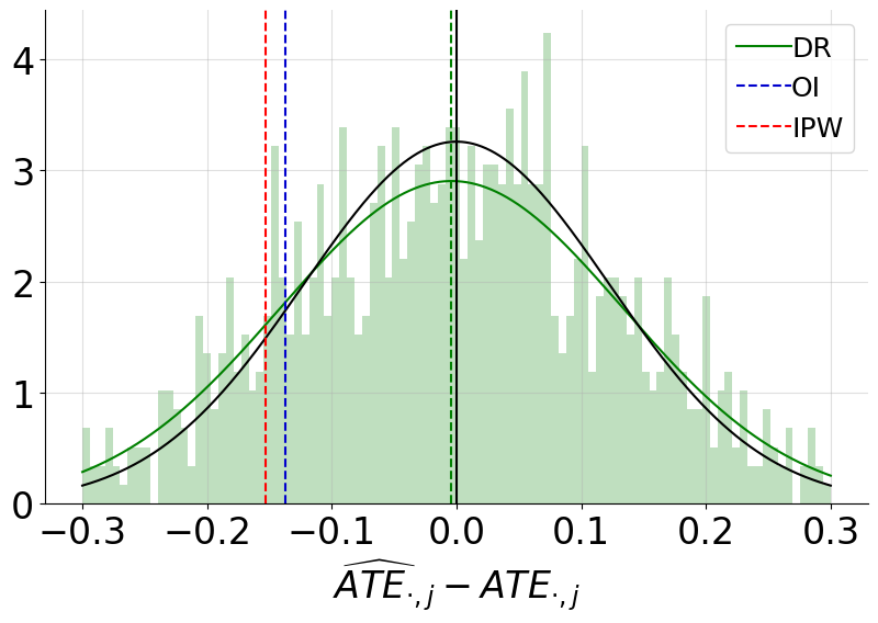
Results. Figure 6 reports simulation results for , with , in Panel , and , in Panel . Figure 2 in Section 3 reports simulation results for . In each case, the figure shows a histogram of the distribution of across simulation instances, along with the best fitting Gaussian distribution (green curve). The histogram counts are normalized so that the area under the histogram integrates to one. Figure 6 plots the Gaussian distribution in the result of Theorem 2 (black curve). The dashed blue, red and green lines in Figures 6 and 2 indicate the values of the means of the OI, IPW, and DR error, respectively, across simulation instances. For reference, we place a black solid line at zero and the black curve represents the Gaussian approximation from Theorem 2. The DR estimator has minimal bias and a close-to-Gaussian distribution. The biases of OI and IPW are non-negligible.
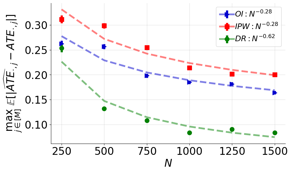
To further illustrate the different bias performance of the three estimators, Figure 7 reports the maximum over of their respective mean absolute error estimates. For each , the estimate of the mean absolute error of OI, IPW, and DR is the average of , and across the simulation instances, respectively. We set and vary . To make the scaling clear, we use least squares to produce the best fit to the maximum bias as varies. We state the empirical decay rates in the legend, e.g., for DR, we report an empirical rate of . The DR estimator consistently outperforms the OI and IPW estimators.
7 Conclusion
This article introduces a new framework to estimate treatment effects in the presence unobserved confounding. We consider modern data-rich environments, where there are many units, and outcomes of interest per unit. We show it is possible to control for the confounding effects of a set of latent variables when this set is low-dimensional relative to the number of observed treatments and outcomes.
Our proposed estimator is doubly-robust, combining outcome imputation and inverse probability weighting with matrix completion. Analytical tractability of its distribution is gained through a novel cross-fitting procedure for matrix completion to estimate the treatment assignment probabilities and mean potential outcomes. We study the properties of the doubly-robust estimator, along with the outcome imputation and inverse probability weighting-based estimators under black-box matrix completion error rates. We show that the decay rate of the mean absolute error for the doubly-robust estimator dominates those of the outcome imputation and the inverse probability weighting estimators. Moreover, we establish a Gaussian approximation to the distribution of the doubly-robust estimator. Simulation results demonstrate the practical relevance of the formal properties of the doubly-robust estimator.
Appendices
Appendix A Supporting Concentration and Convergence Results
This section presents known concentration bounds on subGaussian and subExponential random variables, along with the matrix Hoeffding bound and concludes with a basic result on convergence of random variables.
We use to represent a subGaussian random variable, where is a bound on the subGaussian norm; and to represent a subExponential random variable, where is a bound on the subExponential norm. (Recall the definitions of the norms from Section 1.)
Lemma 1 (subGaussian concentration: Theorem 2.6.3 of Vershynin, (2018)).
Let be a random vector whose entries are independent, zero-mean, random variables Then, for any and ,
| (A.1) |
The following corollary expresses the bound in Lemma 1 in a convenient form.
Corollary 2 (subGaussian concentration).
Let be a random vector whose entries are independent, zero-mean, random variables. Then, for any and any , with probability at least ,
| (A.2) |
Proof.
The proof follows from Lemma 1 by choosing . ∎
Lemma 2 (subExponential concentration: Theorem 2.8.2 of Vershynin, (2018)).
Let be a random vector whose entries are independent, zero-mean, random variables Then, for any and ,
| (A.3) |
The following corollary expresses the bound in Lemma 2 in a convenient form.
Corollary 3 (subExponential concentration).
Let be a random vector whose entries are independent, zero-mean, random variables Then, for any and any , with probability at least ,
| (A.4) |
where recall that .
Proof.
Choosing in Lemma 2, we have
| (A.5) | ||||
| (A.6) |
where the second inequality follows from for any and . Then, the proof follows by choosing which fixes .
∎
Lemma 3 (Product of subGaussians is subExponential: Lemma. 2.7.7 of Vershynin, (2018)).
Let and be and random variables, respectively. Then, is random variable.
Lemma 4 (Matrix Hoeffding bound: Theorem 1.3 of Tropp, (2012)).
Let be a sequence of independent, random, and symmetric matrices such that, for every , and . Let be a sequence of fixed symmetric matrices such that, for every , and is positive semi-definite. Then,
| (A.7) |
In the following corollary, we re-express the bound in Lemma 4 in a convenient form.
Corollary 4 (Matrix Hoeffding bound).
Let be a sequence of independent, random, and symmetric matrices such that, for every , and . Let be a sequence of fixed symmetric matrices such that, for every , and is positive semi-definite. Then, for any , with probability at least ,
| (A.8) |
Proof.
The proof follows from Lemma 4 by choosing . ∎
Next lemma provides a useful intermediate result on convergence in probability.
Lemma 5.
Let and be sequences of random variables such that . Let be a deterministic sequence such that . Suppose . Then, .
Proof.
Consider any . Then, the event belongs to the union of and . Using the union bound,
Then, follows because . ∎
Appendix B Proof of Theorem 1: Finite Sample Guarantees for DR
Fix any . Recall the definitions Eqs. 5 and 16 of the parameters and corresponding doubly robust estimates . The error can be re-expressed as
| (A.9) | ||||
| (A.10) | ||||
| (A.11) |
where follows after defining and for every . Then, we have
| (A.12) | ||||
| (A.13) | ||||
| (A.14) | ||||
| (A.15) | ||||
| (A.16) |
where follows from Eq. 18, and follows from Eqs. 1, 2, and 3. A similar derivation for implies that
| (A.17) | ||||
| (A.18) | ||||
| (A.19) |
Consider any and any . We claim that, with probability at least ,
| (A.20) |
where recall that . We provide a proof of this claim at the end of this section. Applying triangle inequality in Eq. A.11 and using Eq. A.20 with a union bound, we obtain that
| (A.21) |
with probability at least . The claim in Eq. 26 follows by re-parameterizing .
Next, to establish the claim in Eq. 27, choose and note that every term in the right hand side of Eq. A.21 is under the conditions on and . Then, Eq. 27 follows from Lemma 5.
Proof of bound (A.20). Recall the partitioning of the units into and from 4. Condition on this partition. Now, to enable the application of concentration bounds, we split the summation over in the left hand side of Eq. A.20 into two parts—one over and the other over —such that the noise terms are independent of the estimates of in each of these parts as in Eqs. 21 and 22.
Note that . Let . Eq. A.16 and triangle inequality imply
| (A.22) | ||||
| (A.23) |
Applying the Cauchy-Schwarz inequality to bound the first term yields that
| (A.24) | ||||
| (A.33) |
To bound the second term in Eq. A.23, note that is (see Example 2.5.8 in Vershynin, (2018)), zero-mean due to 2(a), and independent across all due to 2(c). Moreover, 4 (i.e., Eq. 21) provides that . Hence, applying the subGaussian concentration (Corollary 2) for yields that
| (A.42) |
with probability at least .
To bound the third term in Eq. A.23, note that is due to 2(e), zero-mean due to 2(a), and independent across all due to 2(d). Moreover, 4 provides (i.e., Eq. 22) that . Hence, applying the subGaussian concentration (Corollary 2) for yields that
| (A.51) |
with probability at least .
Finally, to bound the fourth term in Eq. A.23, note that is due to Lemma 3. Further, is zero-mean due to 2(a) and independent across all due to 2(b), (c), and (d). Moreover, 4 (i.e., Eqs. 21 and 22) imply that . Hence, applying the subExponential concentration (Corollary 3) for yields that
| (A.60) |
with probability at least . Putting together Eqs. A.23, A.33, A.42, A.51, and A.60, we conclude that, with probability at least ,
| (A.77) | ||||
| (A.94) |
Then, noting that for every and from 3, and consequently that for any matrix and every , we obtain the following bound, with probability at least ,
| (A.95) | ||||
| (A.96) | ||||
| (A.97) |
where follows from Eq. 23 and because and . Then, the claim in Eq. A.20 follows for by using Eq. A.97 and applying a union bound over . The proof of Eq. A.20 for follows similarly.
Appendix C Proof of Theorem 2: Asymptotic Normality for DR
For every , recall the definitions of and from Eq. A.16 and Eq. A.19, respectively. Then, define
| (A.98) | ||||
| (A.99) | ||||
| and | ||||
| (A.100) | ||||
Fix any . Then, the simplification of in Eq. A.11 can be re-expressed as
| (A.101) |
We prove in Sections C.1 and C.2 the following convergence results for the above terms.
Lemma 6 (Convergence of ).
Lemma 7 (Convergence of ).
C.1 Proof of Lemma 6
Fix any . Consider any and any . We claim that, with probability at least ,
| (A.104) |
where recall that . We provide a proof of this claim at the end of this section. Then, using Eq. A.104 with a union bound, and the fact that as per condition (C3), we obtain the following with probability at least ,
| (A.105) |
We emphasize that Eq. A.105 holds for any . Next, we choose a particular that is and, under conditions (C1) and (C2), show that each of the three terms in the right hand side of Eq. A.105 are . In particular, we choose
| (A.106) |
We note that this choice of suffices. First, follows by using condition (C1), the continuous mapping theorem, and the convergence in probability of the maximum of two sequences of variables. Second, from condition (C2). Third, follows by using condition (C1) and the continuous mapping theorem after noting that . Fourth, follows by using condition (C1) and the continuous mapping theorem after noting that . Finally, Lemma 6 follows from Lemma 5.
Proof of Eq. A.104 This proof follows a very similar road map to that used for establishing the inequality in display (A.20). Recall the partitioning of the units into and from 4. Condition on this partition. Now, to enable the application of concentration bounds, we split the summation over in the left hand side of Eq. A.104 into two parts—one over and the other over —such that the noise terms are independent of the estimates of in each of these parts as in Eqs. 21 and 22.
Fix . Then, Eqs. A.16 and A.98 imply that
| (A.107) | ||||
| (A.108) |
Now, note that . Fix any . Then, triangle inequality implies that
| (A.109) | ||||
| (A.110) |
Next, note that the decomposition in Eq. A.110 is identical to the one in Eq. A.23, except for the fact when compared to Eq. A.23, the last two terms in Eq. A.110 have an additional factor of . As a result, mimicking steps used to derive Eq. A.94, we can obtain the following bound, with probability at least ,
| (A.127) | ||||
| (A.144) |
Then, noting that and for all and from 3 and 1, and consequently that and for any matrix and every , we obtain the following bound, with probability at least ,
| (A.145) | ||||
| (A.146) | ||||
| (A.147) | ||||
| (A.148) | ||||
| (A.149) |
where follows because from 1 and , and follows from Eq. 23. Then, the claim in Eq. A.104 follows for by applying a union bound over using Eq. A.149, and re-parameterizing . The proof of Eq. A.20 for follows similarly.
C.2 Proof of Lemma 7
To prove this result, we invoke Lyapunov central limit theorem (CLT).
Lemma 8 (Lyapunov CLT, see Theorem 27.3 of Billingsley, (2017)).
Consider a sequence of independent, mean-zero, and finite variance random variables. If Lyapunov’s condition is satisfied, i.e., there exists such that
| (A.150) | |||
| as , then | |||
| (A.151) | |||
as .
Fix any . We apply Lyapunov CLT in Lemma 8 on the sequence where is as defined in Eq. A.100. Note that 2(a) and (b) imply for all , and 2(b), (c), and (d) imply that for all . First, we show in Section C.2.1 that
| (A.152) |
for each . Next, we show in Section C.2.2 that Lyapunov’s condition (A.150) holds for the sequence with . Finally, applying Lemma 8 and using the definition of from Eq. 33 yields Lemma 7.
C.2.1 Proof of Eq. A.152
Fix any and consider . We have
| (A.153) |
We claim the following:
| (A.154) | |||
| (A.155) | |||
| (A.156) |
Then, Eq. A.152 follows by putting together Eqs. A.153, A.154, A.155, and A.156 by using for any random variables and . It remains to establish the claims in Eqs. A.154, A.155, and A.156.
2 immediately implies that and (so that is mean zero). Applying these observations, we obtain Eq. A.154 as follows,
| (A.157) | ||||
| (A.158) | ||||
| (A.159) |
where follows because from Eq. 3, and from condition (C3). A similar argument establishes Eq. A.155. Applying the same observations as above, we obtain Eq. A.156 as follows,
| (A.160) | ||||
| (A.161) | ||||
| (A.162) | ||||
| (A.163) |
where follows because from 2 and follows because from Eq. 3.
C.2.2 Proof of Lyapunov’s condition with
We have
| (A.164) | ||||
| (A.165) | ||||
| (A.166) |
where follows by putting together Eqs. 33 and A.152, follows because as per condition (C3), follows because the absolute third moments of subExponential random variables are bounded, after noting that is a subExponential random variable. Then, condition (A.150) holds for as the right hand side of Eq. A.166 goes to as .
Appendix D Proof of Proposition 1 (28): Finite Sample Guarantees for OI
Fix any . Recall the definitions Eqs. 5 and 12 of the parameters and corresponding outcome imputation estimates . The error can be re-expressed as
| (A.167) | ||||
| (A.168) |
Using the triangle inequality, we have
| (A.169) |
Consider any . We claim that
| (A.170) |
The proof is complete by putting together Eqs. A.169 and A.170.
Appendix E Proof of Proposition 1 (29): Finite Sample Guarantees for IPW
Fix any . Recall the definitions Eqs. 5 and 14 of the parameters and corresponding inverse probability weighting estimates . The error can be re-expressed as
| (A.172) | ||||
| (A.173) | ||||
| (A.174) |
where follows after defining and for every . Then, we have
| (A.175) | ||||
| (A.176) | ||||
| (A.177) | ||||
| (A.178) |
where follows from Eqs. 1, 2, and 3. A similar derivation for implies that
| (A.179) | ||||
| (A.180) | ||||
| (A.181) |
Consider any and any . We claim that, with probability at least ,
| (A.182) |
where recall that . We provide a proof of this claim at the end of this section. Applying triangle inequality in Eq. A.174 and using Eq. A.182 with a union bound, we obtain that
| (A.183) |
with probability at least . The claim in Eq. 29 follows by re-parameterizing .
Proof of Eq. A.182. This proof follows a very similar road map to that used for establishing the inequality in display (A.20). Recall the partitioning of the units into and from 4. Condition on this partition. Now, to enable the application of concentration bounds, we split the summation over in the left hand side of Eq. A.182 into two parts—one over and the other over —such that the noise terms are independent of the estimates of in each of these parts as in Eqs. 21 and 22.
Fix and note that . Fix any . Then, Eq. A.178 and triangle inequality imply that
| (A.184) |
Next, note that the decomposition in Eq. A.184 is identical to the one in Eq. A.23, except for the fact when compared to Eq. A.23, the first two terms in Eq. A.184 have a factor of instead of . As a result, mimicking steps used to derive Eq. A.96, we obtain the following bound, with probability at least ,
| (A.185) | ||||
| (A.186) | ||||
| (A.187) |
where follows because , and , and follows from Eq. 23. Then, the claim in Eq. A.182 follows for by using Eq. A.187 and applying a union bound over . The proof of Eq. A.182 for follows similarly.
Appendix F Proofs of Propositions 2 and 3
In Section F.1, we prove Proposition 2, i.e., we show that the estimates of , , and generated by Cross-Fitted-MC satisfy 4. Next, we prove Proposition 3 implying that the estimates of , , and generated by Cross-Fitted-SVD satisfy the condition (C2) in Theorem 2 as long as .
F.1 Proof of Proposition 2: Guarantees for Cross-Fitted-MC
Consider any matrix completion algorithm MC and any block partition of the set into four blocks as in 4. Fix any .
F.2 Proof of Proposition 3: Guarantees for Cross-Fitted-SVD
To prove this result, we first derive a corollary of Lemma A.1 in Bai and Ng, (2021) for a generic matrix of interest , such that , and apply it to , , and . We impose the following restrictions on and .
Assumption 8.
There exist a constant and a collection of latent factors
| (A.188) |
such that,
-
(a)
satisfies the factorization: ,
-
(b)
and for some positive constant , and
-
(c)
and are positive definite matrices.
Assumption 9.
The noise matrix is such that,
-
(a)
are zero-mean subExponential with the subExponential norm bounded by a constant ,
-
(b)
for every and , and
-
(c)
are mutually independent (across ).
The next result characterizes the entry-wise error in recovering the missing entries of a matrix where all entries in one block are deterministically missing (see the discussion in Section 5.1) using the TW algorithm (summarized in Section 5.2.1). Its proof, essentially established as a corollary of Bai and Ng, (2021, Lemma A.1), is provided in Section F.3.
Corollary 5.
Consider a matrix of interest that satisfies 8 and a noise matrix that satisfies 9. Let be the observed matrix as in Eq. 8. Let and denote the set of rows and columns of , respectively, with all entries observed. Suppose the mask matrix is such that each belongs to with probability and each belongs to with probability . Let where and . Then, produces an estimate of such that
| (A.189) |
as .
Given this corollary, we now complete the proof of Proposition 3. Consider the partition in step 2 of Cross-Fitted-SVD and fix any . Recall that Cross-Fitted-SVD applies TW on , , and , and note that satisfies the requirement on the mask matrix in Corollary 5.
F.2.1 Estimating .
Consider estimating using Cross-Fitted-SVD. To apply Corollary 5, we use 5 and 6 to note that satisfies 8 with rank parameter . Then, we use Eq. 3 and 2(b) to note that satisfies 9. Step 3 of Cross-Fitted-SVD can be rewritten as and where . Then,
| (A.190) |
where follows from 1 and 3, and the definition of , and follows from Corollary 5. Applying a union bound over all , we have
| (A.191) |
where follows from the definition of norm.
F.2.2 Estimating and .
For every , we show that
| (A.192) |
We focus on noting that the proof for is analogous. We split the proof in two cases: (i) and (ii) .
In the first case, we have
| (A.193) | ||||
| (A.194) |
where follows from 3 and follows from the definition of . Then,
| (A.195) |
where follows from the definition of norm, follows from Eq. A.194, and follows from Eq. A.191. Then, Eq. A.192 follows as and are assumed to be bounded.
In the second case, using Eqs. 2 and 3 to expand , we have
| (A.196) |
Next, we utilize two claims proven in Sections F.2.3 and F.2.4 respectively: satisfies 8 with rank parameter and
| (A.197) |
satisfies 9.
Now, note that step 6 of Cross-Fitted-SVD can be rewritten as and where . Then, from Corollary 5,
| (A.198) |
Applying a union bound over all and noting that , we have
| (A.199) |
The left hand side of Eq. A.199 can be written as,
| (A.200) | ||||
| (A.201) | ||||
| (A.202) |
where follows from triangle inequality as and follows from 3 and the definition of . Then,
| (A.203) | ||||
| (A.204) |
where follows from the definition of norm, follows from Eq. A.202, and follows from Eqs. A.191 and A.199. Then, Eq. A.192 follows as and are assumed to be bounded.
F.2.3 Proof that and satisfy 8.
Recall the factors and of , and and of from Section 5.3. Then, 8(a) holds from Eq. 49. Next, we note that
| (A.205) |
where follows from the definition of Khatri-Rao product (see Section 1), and follows from 6. Then, satisfies 8(b) by using similar arguments on . Further, satisfies 8(b) by noting that and are bounded whenever and are bounded, respectively. Finally, 8(c) holds from 6.
F.2.4 Proof that satisfies 9
Recall that . Then, 9(a) holds as is zero-mean from 2 and Eq. 3, and is subExponential because is a subExponential random variable Lemma 3, every subGaussian random variable is subExponential random variable, and sum of subExponential random variables is a subExponential random variable. Next, 9(b) holds as
| (A.206) |
where follows from 2, and follows from 2, 7, and 1, Eq. 3, Lemma 3, and because are bounded. Finally, 9(b) holds from 2 and 7.
F.3 Proof of Corollary 5
Corollary 5 is a direct application of Bai and Ng, (2021, Lemma A.1), specialized to our setting. Notably, Bai and Ng, (2021) make four assumptions numbered A, B, C and D in their paper to establish the corresponding result. It remains to establish that the conditions assumed in Corollary 5 imply the necessary conditions used in the proof of Bai and Ng, (2021, Lemma A.1). First, note that due to the specific sampling assumed in defining the mask matrix in Corollary 5, Bai and Ng, (2021, Assumption D) holds immediately and Bai and Ng, (2021, Assumption B) holds with high probability by Hoeffding’s inequality.
It remains to show how 8 and 9 imply the remainder of their assumptions, namely Bai and Ng, (2021, Assumptions A and C). Before doing that, note that certain assumptions in Bai and Ng, (2021) are not actually used in their proof of Lemma A.1 (or in the proof of other results used in that proof), namely, the distinct eigenvalue condition in Assumption A(a)(iii), the asymptotic normality conditions in Assumption A(c) and the asymptotic normality conditions in Assumption C. For completeness, the remaining relevant conditions from Bai and Ng, (2021) are collected in the following two assumptions.
Assumption 10 (Strong block factors).
Consider the latent factors and from 8. Define the following matrices:
| (A.207) |
where and denote the set of rows and columns of , respectively, with all entries observed, and and . Then, the matrices defined below are positive definite:
| (A.208) |
Assumption 11.
The noise matrix is such that,
-
(a)
,
-
(b)
and ,
-
(c)
, and
-
(d)
.
10 is a restatement of Bai and Ng, (2021, Assumption C) (without the central limit theorems, which are not used in Bai and Ng, (2021, Proof of Lemma A.1) as noted above). This condition ensures a strong factor structure on the sub-matrix corresponding to observed elements of as well as on the sub-matrix corresponding to missing elements of .
11 is a restatement of the subset of conditions from Bai and Ng, (2021, Assumption A) necessary in Bai and Ng, (2021, proof of Lemma A.1) and it essentially requires weak dependence in the noise across measurements and across units. In particular, 11(a), (b), (c), and (d) correspond to Assumption A(b)(ii), (iii), (iv), (v), respectively, of Bai and Ng, (2021). For the other conditions in Bai and Ng, (2021, Assumption A), note that 8 above is equivalent to their Assumption A(a)(i) and (ii) of Bai and Ng, (2021) when the factors are non-random as in this work. Similarly, 9(a) above is analogous to Assumption A(b)(i) of Bai and Ng, (2021). Assumption A(b)(vi) of Bai and Ng, (2021) is implied by their other Assumptions for non-random factors as stated in Bai, (2003).
To establish Corollary 5, it remains to establish that 10 and 11 hold, which is done in Sections F.3.1 and F.3.2 respectively.
F.3.1 10 holds
We show that is positive definite. The proof for , , and being positive definite follows similarly. Define . From Weyl’s inequality (Bhatia,, 2007, Theorem. 8.2), we have the following for some :
| (A.209) | ||||
| (A.210) |
where follows from 8(c) as is positive definite. Now, it suffices to show that .
Recall that the mask matrix is such that each belongs to with probability . For every , let be an indicator random variable such that if and if . Then, we express as follows,
| (A.211) |
Then, we have
| (A.212) | ||||
| (A.213) | ||||
| (A.214) |
where follows from Eq. A.211 and the definition of , and follows from the triangle inequality on the operator norm after noting that the maximum eigenvalue of any symmetric matrix coincides with its operator norm. Next, we show that each term in Eq. A.214 is .
Proof that first term in Eq. A.214 is . We have
| (A.215) |
To bound Eq. A.215, we apply Corollary 4 with
| (A.216) |
We note that, for every , as and is positive semi-definite as
| (A.217) |
where follows because . We claim that for some . Then, using Corollary 4, Eq. A.215 is bounded as follows with probability at least ,
| (A.218) |
Therefore, the first term in Eq. A.214 is . It remains to bound . We have
| (A.219) | ||||
| (A.220) | ||||
| (A.221) | ||||
| (A.222) |
where follows from the definition of the maximum eigenvalue of a matrix, follows from Eq. A.216, follows because , and follow from 8(b), follows from Cauchy-Schwarz inequality.
Proof that second term in Eq. A.214 is . We have
| (A.223) |
To bound Eq. A.223, we claim for some , and apply Corollary 2 on the vector . We note that, for every , is zero-mean and (see Example 2.5.8 in Vershynin, (2018)). Then, with probability at least ,
| (A.224) |
Using Eq. A.224 to bound Eq. A.223, with probability at least , we have
| (A.225) |
Therefore, the first term in Eq. A.214 is . It remains to bound . We have
| (A.226) | ||||
| (A.227) | ||||
| (A.228) |
where follows from the definition of the maximum eigenvalue of a matrix, follows from Cauchy-Schwarz inequality, and follows from 8(b).
F.3.2 11 holds
First, 11(a) holds as follows,
| (A.229) |
where follows from triangle inequality and follows from 9(b). Next, from 9(a) and 9(c), we have
| (A.230) |
| (A.231) |
| (A.232) |
where follows from 9(c) and follows from 9(b). Next, let and fix any . Then, 11(d) holds as follows,
| (A.233) | ||||
| (A.234) |
where follows from linearity of expectation and 9(c) after by noting that for all and follows because has bounded moments due to 9(a).
Appendix G Data generating process for the simulations
The inputs of the data generating process (DGP) are: the probability bound ; two positive constants and ; and the standard deviations for every . The DGP is:
-
1.
For positive integers , and , generate a proxy for the common unit-level latent factors , such that, for all and , is independently sampled from a distribution, with .
-
2.
Generate proxies for the measurement-level latent factors , such that, for all and , are independently sampled from a distribution.
-
3.
Generate the treatment assignment probability matrix
(A.235) -
4.
For , run SVD on , i.e.,
(A.236) Then, generate the mean potential outcome matrices and :
(A.237) where denotes the sum of all entries of .
-
5.
Generate the noise matrices and , such that, for all , is independently sampled from a distribution. Then, determine from Eq. 2.
- 6.
In our simulations, we set , and . In practice, instead of choosing the values of as ex-ante inputs, we make them equal to the standard deviation of all the entries in for every and , separately for .
References
- Abadie et al., (2010) Abadie, A., Diamond, A., and Hainmueller, J. (2010). Synthetic control methods for comparative case studies: Estimating the effect of california’s tobacco control program. Journal of the American Statistical Association, 105(490):493–505.
- Abadie and Imbens, (2006) Abadie, A. and Imbens, G. W. (2006). Large sample properties of matching estimators for average treatment effects. Econometrica, 74(1):235–267.
- (3) Agarwal, A., Dahleh, M., Shah, D., and Shen, D. (2023a). Causal matrix completion. In The Thirty Sixth Annual Conference on Learning Theory, pages 3821–3826. PMLR.
- (4) Agarwal, A., Shah, D., and Shen, D. (2023b). Synthetic interventions.
- Agarwal et al., (2021) Agarwal, A., Shah, D., Shen, D., and Song, D. (2021). On robustness of principal component regression. Journal of the American Statistical Association, pages 1–34.
- Angrist, (1998) Angrist, J. D. (1998). Estimating the labor market impact of voluntary military service using social security data on military applicants. Econometrica, 66(2):249–288.
- Arkhangelsky et al., (2021) Arkhangelsky, D., Athey, S., Hirshberg, D. A., Imbens, G. W., and Wager, S. (2021). Synthetic difference-in-differences. American Economic Review, 111(12):4088–4118.
- Athey et al., (2021) Athey, S., Bayati, M., Doudchenko, N., Imbens, G., and Khosravi, K. (2021). Matrix completion methods for causal panel data models. Journal of the American Statistical Association, 116(536):1716–1730.
- Bai, (2003) Bai, J. (2003). Inferential theory for factor models of large dimensions. Econometrica, 71(1):135–171.
- Bai, (2009) Bai, J. (2009). Panel data models with interactive fixed effects. Econometrica, 77(4):1229–1279.
- Bai and Ng, (2002) Bai, J. and Ng, S. (2002). Determining the number of factors in approximate factor models. Econometrica, 70(1):191–221.
- Bai and Ng, (2021) Bai, J. and Ng, S. (2021). Matrix completion, counterfactuals, and factor analysis of missing data. Journal of the American Statistical Association, 116(536):1746–1763.
- Bang and Robins, (2005) Bang, H. and Robins, J. M. (2005). Doubly robust estimation in missing data and causal inference models. Biometrics, 61(4):962–972.
- Bhatia, (2007) Bhatia, R. (2007). Perturbation bounds for matrix eigenvalues. SIAM.
- Bhattacharya and Chatterjee, (2022) Bhattacharya, S. and Chatterjee, S. (2022). Matrix completion with data-dependent missingness probabilities. IEEE Transactions on Information Theory, 68(10):6762–6773.
- Billingsley, (2017) Billingsley, P. (2017). Probability and measure. John Wiley & Sons.
- Chatterjee, (2015) Chatterjee, S. (2015). Matrix estimation by universal singular value thresholding. The Annals of Statistics, 43(1):177 – 214.
- Chernozhukov et al., (2018) Chernozhukov, V., Chetverikov, D., Demirer, M., Duflo, E., Hansen, C., Newey, W., and Robins, J. (2018). Double/debiased machine learning for treatment and structural parameters. The Econometrics Journal, 21(1):C1–C68.
- Cochran, (1968) Cochran, W. G. (1968). The effectiveness of adjustment by subclassification in removing bias in observational studies. Biometrics, pages 295–313.
- (20) Dwivedi, R., Tian, K., Tomkins, S., Klasnja, P., Murphy, S., and Shah, D. (2022a). Counterfactual inference for sequential experiments. arXiv preprint arXiv:2202.06891.
- (21) Dwivedi, R., Tian, K., Tomkins, S., Klasnja, P., Murphy, S., and Shah, D. (2022b). Doubly robust nearest neighbors in factor models. arXiv preprint arXiv:2211.14297.
- Imbens and Rubin, (2015) Imbens, G. W. and Rubin, D. B. (2015). Causal Inference for Statistics, Social, and Biomedical Sciences: An Introduction. Cambridge University Press.
- Li et al., (2019) Li, Y., Shah, D., Song, D., and Yu, C. L. (2019). Nearest neighbors for matrix estimation interpreted as blind regression for latent variable model. IEEE Transactions on Information Theory, 66(3):1760–1784.
- Ma and Chen, (2019) Ma, W. and Chen, G. H. (2019). Missing not at random in matrix completion: The effectiveness of estimating missingness probabilities under a low nuclear norm assumption. Advances in neural information processing systems, 32.
- Nguyen et al., (2019) Nguyen, L. T., Kim, J., and Shim, B. (2019). Low-rank matrix completion: A contemporary survey. IEEE Access, 7:94215–94237.
- Rosenbaum and Rubin, (1983) Rosenbaum, P. R. and Rubin, D. B. (1983). The central role of the propensity score in observational studies for causal effects. Biometrika, 70(1):41–55.
- Tropp, (2012) Tropp, J. A. (2012). User-friendly tail bounds for sums of random matrices. Foundations of computational mathematics, 12:389–434.
- Vershynin, (2018) Vershynin, R. (2018). High-dimensional probability: An introduction with applications in data science, volume 47. Cambridge university press.