Spectral Independence Beyond Uniqueness with
the topological method - An extended view -

Abstract.

We present novel results for fast mixing of Glauber dynamics using the newly introduced and powerful Spectral Independence method from [Anari, Liu, Oveis-Gharan: FOCS 2020]. We mainly focus on the Hard-core model and the Ising model.

We obtain bounds for fast mixing with the parameters expressed in terms of the spectral radius of the adjacency matrix, improving on the seminal work in [Hayes: FOCS 2006]. Furthermore, we go beyond the adjacency matrix and establish -for the first time- rapid mixing results for Glauber dynamics expressed in terms of the spectral radius of the Hashimoto non-backtracking matrix of the underlying graph $G$.

Working with the non-backtracking spectrum is extremely challenging, but also more desirable. Its eigenvalues are less correlated with the high-degree vertices than those of the adjacency matrix and express more accurately invariants of the graph such as the growth rate. Our results require “weak normality” from the Hashimoto matrix. This condition is mild and allows us to obtain very interesting bounds.

We study the pairwise influence matrix ${{\mathcal{I}}}^{\Lambda,\tau}_{G}$ by exploiting the connection between the matrix and the trees of self-avoiding walks, however, we go beyond the standard treatment of the distributional recursions. The common framework that underlies our techniques we call the topological method.

Our approach is novel and gives new insights into how to establish Spectral Independence for Gibbs distributions. More importantly, it allows us to derive new -improved- rapid mixing bounds for Glauber dynamics on distributions such as the Hard-core model and the Ising model for graphs that the spectral radius is smaller than the maximum degree.

1. Introduction

The Markov Chain Monte Carlo method (MCMC) is a very simple, yet very powerful method for approximate sampling from Gibbs distributions on combinatorial structures. In the standard setting, we are given a very simple to describe, ergodic Markov chain and we need to analyse the speed of convergence to the equilibrium distribution. The challenge is to show that the chain mixes fast when the parameters of the equilibrium distribution belong to a certain region of values.

Here our focus is on combinatorial structures that are specified with respect to an underlying graph $G$, such as the independent sets. For us, the graph $G$ is always simple, connected and finite. Also, we assume that the corresponding matrices we obtain from $G$ are irreducible.

The Spectral Independence is a (newly) introduced technique for analysing the speed of convergence of the well-known Markov chain called Glauber dynamics. It has been proposed in [3] and builds on results for high dimensional expanders, such as [2]. The authors in [3] use the Spectral Independence method (SI) to prove a long-standing conjecture about the mixing time of Glauber dynamics for the so-called Hard-core model, improving on a series of results such as [20, 39]. Since then, it is not an exaggeration to claim that SI has revolutionised the study in the field. Using this method it has been possible to get positive results for approximate sampling from 2-spin Gibbs distributions that match the hardness ones, e.g., [3, 8, 9, 11, 37, 38].

In this work, our main focus is on the so-called pairwise influence matrix, denoted as ${{\mathcal{I}}}^{\Lambda,\tau}_{G}$. This is a central concept for SI as the rapid mixing bounds we obtain with this method rely on showing that the maximum eigenvalue of this matrix is bounded.

We provide a novel perspective on how to analyse ${{\mathcal{I}}}^{\Lambda,\tau}_{G}$ and this allows us to derive more accurate estimations on the maximum eigenvalue of this matrix than what we have been getting from previous works such as [3, 11]. We study the pairwise influence matrix ${{\mathcal{I}}}^{\Lambda,\tau}_{G}$ by exploiting the connection between the matrix and the trees of self-avoiding walks, however, we go beyond the standard treatment of the distributional recursions. Interestingly, in our results the fast mixing regions for Glauber dynamics do not depend on the maximum degree ${\Delta}$ of the underlying graph $G$, they rather depend on the spectrum of $G$. Specifically, we present a set of results expressed in terms of the spectral radius of the adjacency matrix _G. We further present results expressed in terms of the spectral radius of the Hashimoto non-backtracking matrix _G.

The non-backtracking matrix _G is less studied compared to the adjacency matrix _G. It originates from physics and was introduced in [24]. It is a very interesting object to work with. In the recent years, it has found many applications in computer science e.g.,[1, 6, 14, 30, 32]. One of its desirable properties is that the eigenvalues of _G tend to be less correlated to the high-degree vertices of the graph, i.e., compared to _G. In many cases of interest, they are mostly related to the expected degree of the graph, e.g. see [6]. Working with _G is the natural step to consider beyond the adjacency matrix. On the other hand, it is very challenging to work with _G. It is not symmetric, i.e., it is over the oriented edges of $G$. Many standard tools from linear algebra do not apply here. Hence, even basic questions about this matrix might be extremely difficult to answer.

We focus on two-spin Gibbs distributions and get new rapid mixing results for the Glauber dynamics for the Hard-core model and the Ising model improving on the seminal work of Hayes in [25]. It turns out that the classification of rapid mixing results with respect to the spectrum of $G$ is more precise than that with the maximum degree ${\Delta}$. In that respect, our results refine the connection between the hardness of counting and the rapid mixing of Glauber dynamics, indicating that the hard cases correspond to graphs with large spectral radii.

For the adjacency matrix, we prove results of the following flavour: consider the Glauber dynamics on the Hard-core model for $G$ whose adjacency matrix has spectral radius ${\rho}$. Let ${\lambda_{c}}(k)$ be the critical value for the Gibbs uniqueness of the Hard-core model on the infinite $k$-ary tree. We prove mixing time $O(n\log n)$ for Glauber dynamics for any $0\leq\lambda<{\lambda_{c}}({\rho})$.

For comparison, recall that the max-degree-${\Delta}$ bound for the Hard-core model requires fugacity $0\leq\lambda<{\lambda_{c}}({\Delta}-1)$ to get $O(n\log n)$ mixing time. This implies that our approach gives better bounds when the spectral radius ${\rho}$ is smaller than ${\Delta}-1$. As a reference, note that we always have that ${\rho}\leq{\Delta}$. On the other hand, the spectral radius can get much smaller than the maximum degree, e.g., for a planar graph, we have that ${\rho}\leq\sqrt{8{\Delta}-16}+2\sqrt{3}$, while we have similar behaviour ${\rho}=O(\sqrt{{\Delta}})$ for graphs of small Euler genus, see further discussions in Section 2.1. We obtain bounds expressed in terms of ${\rho}({}_{G})$ for the Ising model, too.

The idea to utilise the spectrum of _G (or matrix norms) to obtain rapid mixing bounds is not new in the literature, i.e., it originates from [25] and was further developed in [15, 26]. Our results here improve on [25]. The improvement in the parameters of the Gibbs distributions is as large as a constant factor. As opposed to our approach that utilises SI, these earlier results rely on the path coupling technique [7]. Our improvement reflects the fact that SI is stronger than path coupling.

As opposed to _G, obtaining bounds in terms of _G has not been considered before in the literature. Note that _G is a completely different object to work with, while the analysis is more intricate. The results we obtain are of similar flavour to those for _G. E.g. for the Hard-core model, we show mixing time $O(n\log n)$ for the Glauber dynamics for any fugacity $0<\lambda<\lambda_{c}({\rho})$ where now ${\rho}={\rho}({}_{G})$. In our results we have the mild requirement that _G is “weakly normal”. This means that we need to have ${\uppsi}_{1}(e)/{\upkappa}_{1}(e)=\Theta(1)$ for all the entries of ${\uppsi}_{1}$, ${\upkappa}_{1}$, the left and right principal eigenvectors of _G, respectively.

One way of having weak normality is by allowing backtracking after a bounded number of steps, i.e., for every oriented edge $e$ of $G$, there is a bounded number $\ell>0$ such that ${}^{\ell}_{G}(e,e^{-1})>0$, where $e,e^{-1}$ is the oriented edge and its reverse. Somehow, backtracking after a bounded number of steps is in contrast to what we have with _G, where we need to allow backtracking within one step.

Interesting cases of graphs with weak-normality include, e.g., the planar graph where each vertex belongs to at least one face of bounded degree. The strength of the results for _G is particularly evident when the underlying graph $G$ is of large girth and average degree $d\ll{\Delta}$. In this setting it is standard to come up with cases such that ${\rho}({}_{G})\ll{\rho}({}_{G})$. For example, consider the graph $G$ of bounded average degree $d$ and girth $g$, e.g. say $g={\rm poly}(\log d)$, while assume that $d$ is a large number. Suppose that the maximum degree is $d^{100}$, while for each vertex in the graph, the number of neighbours at distance $g/2$ is $\leq d^{g/2}$. Then, it is not hard to show that ${\rho}({}_{G})\leq d$. Furthermore, if $G$ is weakly normal, the rapid mixing bound we obtain for the Hard-core model on $G$ is roughly $\lambda<e/d$, i.e., $d$ is the average degree. For comparison, the corresponding bound for the adjacency matrix cannot get better than $\lambda<\frac{e}{\sqrt{{\Delta}}}=\frac{e}{d^{50}}$, while the maximum degree bound is $\lambda<e/d^{100}$.

It is worth mentioning that apart from the challenges that emerge from the analysis of matrix _G, it is also challenging to accommodate in the analysis the high-degree vertices. This is similar to e.g., [5, 18, 19, 36]. In that respect, we utilise results from [36]. The obstacle in applying our results to multi-spin distributions such as the graph colourings, or its generalisation the Potts model comes from the fact that we still do not know how to deal with the effect of high degree vertices for these distributions, i.e., despite the recent advances in the area [4, 10].

Establishing Spectral Independence - The Topological Method

A natural question at this point is how the eigenvalues of the matrix of interest, i.e., _G, or _G, emerge in the analysis. The starting point is the following, well-known, observation: each entry ${{\mathcal{I}}}^{\Lambda,\tau}_{G}(w,v)$ can be expressed in terms of a topological construction called the tree of self-avoiding walks (starting from $w$), together with a set of weights on the paths of this tree, which are called influences. The influences are specified by the parameters of the Gibbs distribution we consider. Essentially, the entry of the influence matrix is nothing more than the sum of influences over an appropriately chosen set of paths in this tree.

In that respect, it is implicit in our approach that we approximate the tree of self-avoiding walks with other topological constructions such as path-trees, universal covers (e.g. see [23]). The aim of these constructions is to obtain a “larger” matrix than ${{\mathcal{I}}}^{\Lambda,\tau}_{G}$, i.e., with a larger spectral radius, that is easier to analyse. For most of the cases, the spectral radius emerges by introducing weights on the tree recursions that typically emerge in the analysis. The weights are from the (right) principal eigenvector of the corresponding graph matrix.

2. Results

Consider the graph $G=(V,E)$ on $n$ vertices. We assume that $G$ is simple, finite and connected, while the maximum degree ${\Delta}$ is bounded. The Gibbs distribution $\mu$ on $G$ with spins $\{\pm 1\}$ is a distribution on the set of configurations $\{\pm 1\}^{V}$. We use the parameters $\beta\in\mathbb{R}_{\geq 0}$ and $\gamma,\lambda\in\mathbb{R}_{>0}$ and specify that each configuration $\sigma\in\{\pm 1\}^{V}$ gets a probability measure

$$\mu(\sigma) \propto\textstyle\lambda^{\#\textrm{assignments ``1" in $\sigma$ }}\times\beta^{\#\textrm{edges with both ends ``1" in $\sigma$ }}\times\gamma^{\#\textrm{edges with both ends ``-1" in $\sigma$}},$$ (2.1)

where the symbol $\propto$ stands for “proportional to”.

The above distribution is called ferromagnetic when $\beta\gamma>1$, while for $\beta\gamma<1$ it is called antiferromagnetic. Unless otherwise specified, we always assume that $\mu$ is a two-spin Gibbs distribution.

Using the formalism in (2.1), one recovers the Ising model by setting $\beta=\gamma$. In this case, the magnitude of $\beta$ specifies the strength of the interactions. The above, also, gives rise to the so-called Hard-core model if we choose $\beta=0$ and $\gamma=1$. Particularly, this distribution assigns to each independent set $\sigma$ probability mass which is proportional to $\lambda^{|\sigma|}$, where $|\sigma|$ is the size of the independent set. We use the term fugacity to refer to the parameter $\lambda$ of the Hard-core model.

Glauber Dynamics.

Given a Gibbs distribution $\mu$, we use the discrete-time, (single site) Glauber dynamics ${\{X_{t}\}_{t\geq 0}}$ to approximately sample from $\mu$. Glauber dynamics is a very simple to describe Markov chain. The state space is the support of $\mu$. We assume that the chain starts from an arbitrary configuration $X_{0}$. For $t\geq 0$, the transition from the state $X_{t}$ to $X_{t+1}$ is according to the following steps: Choose uniformly at random a vertex $v$. For every vertex $w$ different than $v$, set $X_{t+1}(w)=X_{t}(w)$. Then, set $X_{t+1}(v)$ according to the marginal of $\mu$ at $v$, conditional on the neighbours of $v$ having the configuration specified by $X_{t+1}$.

For the distributions we consider here, ${\{X_{t}\}_{t\geq 0}}$ satisfies a set of technical conditions that come with the name ergodicity. Ergodicity implies that ${\{X_{t}\}_{t\geq 0}}$ converges to a unique stationary distribution which, in our case, is the Gibbs distribution $\mu$.

We focus on obtaining rapid mixing bounds for Glauber dynamics that depend on the spectral radii of the adjacency matrix _G and the Hashimoto non-backtracking matrix _G of the underlying graph $G$, respectively. These matrices are defined as follows:

Adjacency matrix _G:

For graph $G=(V,E)$, the adjacency matrix _G is a zero-one, $V\times V$ matrix such that for every pair $u,w\in V$ we have that

$${}_{G}(u,w)=\mathds{1}\{\textrm{ $u,w$ are adjacent in $G$}\}\enspace.$$

In our results, we assume that the _G is irreducible. This implies that the underlying graph $G$ needs to be connected.

Figure 1. Oriented edges

Hashimoto non-backtracking matrix

For the graph $G=(V,E)$, let $M$ be the set of oriented edges obtained by doubling each edge of $E$ into two directed edges, i.e., one edge for each direction. The non-backtracking matrix, denoted as _G, is an $M\times M$, zero-one matrix such that for any pair of oriented edges $e=uw$ and $f=zy$, we have that

$${}_{G}(e,f) =\mathds{1}\{w=z\}\times\mathds{1}\{u\neq y\}\enspace.$$

That is, $\UpH(e,f)$ is equal to $1$, if $f$ follows the edge $e$ without creating a loop, otherwise, it is equal to zero. The reader may consider the example in Fig. 1, There, we have ${}_{G}(e,f)={}_{G}(f^{-1},e^{-1})=1$, while ${}_{G}(e,f^{-1})={}_{G}(f^{-1},e)=0$.

For _G irreducibility implies that for any two oriented edges $e,f$, the graph $G$ has a non-backtracking path that connects them. It is standard that _G is irreducible if $G$ is not a cycle and the minimum degree is at least $2$, e.g., see [22].

Ising Model

It is a well-known result that the uniqueness region of the Ising model on the infinite $k$-ary tree, where $k\geq 2$, corresponds to having

$$\frac{k-1}{k+1}<\beta<\frac{k+1}{k-1}\enspace.$$

The uniqueness for the ferromagnetic Ising corresponds to having $1\leq\beta<\frac{k+1}{k-1}$, while for the antiferromagnetic corresponds to having $\frac{k-1}{k+1}<\beta\leq 1$.

For $d>1$ and $\delta\in(0,1)$, we let the interval

$${\mathbb{U}_{\rm Ising}}(d,\delta)=\textstyle\left[\frac{d-1+\delta}{d+1-\delta},\frac{d+1-\delta}{d-1+\delta}\right]\enspace.$$ (2.2)

Theorem 2.1 (Ising Model - Adjacency Matrix).

For any fixed $\varepsilon\in(0,1)$, for bounded ${\rho}>1$, consider the graph $G=(V,E)$ such that the adjacency matrix _G is of spectral radius ${\rho}$. Let $\mu$ be the Ising model on $G$ with zero external field and parameter $\beta\in{\mathbb{U}_{\rm Ising}}({\rho},\varepsilon)$.

There is a constant $C={C(\varepsilon)}$ such that the mixing time of the Glauber dynamics on $\mu$ is at most $Cn\log n$.

Note that having bounded ${\rho}({}_{G})$, implies that ${\Delta}$ is also bounded. This follows from the standard inequality that $\sqrt{{\Delta}}\leq{\rho}({}_{G})$.

We now consider our results for the Hashimoto non-backtracking matrix. As opposed to _G which is a symmetric matrix, _G is not necessarily normal, i.e., in general we have that ${}_{G}\cdot\bar{\UpH}_{G}\neq\bar{\UpH}_{G}\cdot{}_{G}$, where $\bar{\UpH}_{G}$ is the transpose of _G.

For integer $n>0$ and ${\hat{c}}>0$, let ${\mathbb{H}}_{n,{\hat{c}}}$ be the set of irreducible, non-backtracking matrices _G on a graph $G$ with $n$ vertices, such that for any oriented edge $e$, we have that

$$\frac{{\uppsi}_{1}(e)}{{\upkappa}_{1}(e)}\leq{\hat{c}}\enspace,$$ (2.3)

where ${\uppsi}_{1},{\upkappa}_{1}$ are the left and right principal eigenvectors of _G, respectively.

In our results, we assume that _G is weakly normal. This essentially corresponds to having ${}_{G}\in{\mathbb{H}}_{n,{\hat{c}}}$, for ${\hat{c}}=\Theta(1)$.

Theorem 2.2 (Ising Model - Hashimoto Matrix).

For any fixed $\varepsilon\in(0,1)$, for bounded numbers ${\hat{c}}>0$, $\uptheta>1$ and ${\Delta}>1$, consider the graph $G=(V,E)$ of maximum degree ${\Delta}$, such that the Hashimoto matrix ${}_{G}\in{\mathbb{H}}_{n,{\hat{c}}}$, while it has spectral radius $\uptheta$. Let $\mu$ be the Ising model on $G$ with zero external field and parameter $\beta\in{\mathbb{U}_{\rm Ising}}(\uptheta,\varepsilon)$.

There is a constant $C={C(\varepsilon,{\hat{c}})}$ such that the mixing time of the Glauber dynamics on $\mu$ is at most $Cn\log n$.

For the above result, note that assuming that ${\rho}({}_{G})$ is bounded does not imply that ${\Delta}$ is also bounded, i.e., as we had for the adjacency matrix.

Furthermore, it is worth mentioning that the left and right eigenvectors ${\uppsi}_{1},{\upkappa}_{1}$ of _G satisfy that ${\uppsi}_{1}(e)={\upkappa}_{1}(e^{-1})$, for all oriented edges $e$. With this observation in mind, Claim 4.7 implies that if for every oriented edge $e$ there is a bounded number $\ell>0$ such that ${}_{G}^{\ell}(e,e^{-1})>0$, then matrix _G is weakly normal.

Hard-core Model

For $z>1$, we let the function ${\lambda_{c}}(z)=\frac{z^{z}}{(z-1)^{(z+1)}}$. It is a well-known result from [29] that the uniqueness region of the Hard-core model on the $k$-ary tree, where $k\geq 2$, corresponds to having

$$\lambda<{\lambda_{c}}(k)\enspace.$$ (2.4)

As far as the Hard-core model is concerned we derive the following results.

Theorem 2.3 (Hard-core Model - Adjacency Matrix ).

For any fixed $\varepsilon\in(0,1)$, for bounded ${\rho}>1$, consider the graph $G=(V,E)$ such that the adjacency matrix _G has spectral radius ${\rho}$. Also, let $\mu$ be the Hard-core model on $G$ with fugacity $\lambda\leq(1-\varepsilon){\lambda_{c}}({\rho})$.

There is a constant $C={C(\varepsilon)}$ such that the mixing time of the Glauber dynamics on $\mu$ is at most $Cn\log n$.

For the non-backtracking matrix we obtain the following result.

Theorem 2.4 (Hard-core Model - Hashimoto Matrix).

For any fixed $\varepsilon\in(0,1)$, for bounded numbers ${\Delta}\geq 2$, ${\hat{c}}>0$ and $\uptheta>1$, consider the graph $G=(V,E)$ of maximum degree ${\Delta}$, such that the Hashimoto matrix ${}_{G}\in{\mathbb{H}}_{n,{\hat{c}}}$, while it has spectral radius $\uptheta$. Also, let $\mu$ be the Hard-core model on $G$ with fugacity $\lambda\leq(1-\varepsilon){\lambda_{c}}(\uptheta)$.

There is a constant $C={C(\varepsilon,{\hat{c}})}$ such that the mixing time of the Glauber dynamics on $\mu$ is at most $Cn\log n$.

Notation

For the graph $G=(V,E)$ and the Gibbs distribution $\mu$ on the set of configurations $\{\pm 1\}^{V}$. For a configuration $\sigma$, we let $\sigma(\Lambda)$ denote the configuration that $\sigma$ specifies on the set of vertices $\Lambda$. We let $\mu_{\Lambda}$ denote the marginal of $\mu$ at the set $\Lambda$. We let $\mu(\cdot\ |\ M,\sigma)$ and $\mu^{M,\sigma}$ denote the distribution $\mu$ conditional on the configuration at $M\subset V$ being $\sigma$. Also, we interpret the conditional marginal $\mu_{\Lambda}(\cdot\ |\ M,\sigma)$ in the natural way. Similarly, for $\mu^{M,\sigma}_{\Lambda}$.

For the graph $G$ and for $w\in V$, we let $N_{G}(w)$ be the set of vertices which are adjacent to $w$ in the graph. Also, for the integer $N>0$, we let the set $[N]=\{1,2,\ldots,N\}$.

2.1. Applications

There are a lot of interesting cases of graphs whose adjacency matrix has spectral radius much smaller than the maximum degree, and hence, our results give better rapid mixing bounds than the general one. A standard example is the planar graphs for which we have the following bounds on their spectral radius from [17].

Theorem 2.5 ([17]).

Suppose that $G=(V,E)$ is a planar graph of maximum degree ${\Delta}$, then ${\rho}({}_{G})\leq\varrho({\Delta})$where

$$\varrho({\Delta}) =\left\{\begin{array}[]{lcl}{\Delta}&&\textrm{for ${\Delta}\leq 5$}\enspace,\\ \sqrt{12{\Delta}-36}&&\textrm{for $6\leq{\Delta}\leq 36$}\enspace,\\ \sqrt{8({\Delta}-2)}+2\sqrt{3}&&\textrm{for $37\leq{\Delta}$}\enspace.\end{array}\right.$$ (2.8)

In what follows, we show the implications of the above theorem to the mixing time of Glauber dynamics for the Ising model and the Hard-core model. We focus on results for graphs of bounded maximum degree.

As far as the Ising model on planar graphs is concerned, we have the following result.

Corollary 2.6 (Planar Ising model).

For $\delta\in(0,1)$, for fixed ${\Delta}\geq 2$, let the planar graph $G=(V,E)$ be of maximum degree ${\Delta}$. Let $\mu$ be the zero external field Ising model on $G$ with parameter $\beta$ such that

$$\beta\in{\mathbb{U}_{\rm Ising}}\left(\varrho({\Delta}),\delta\right)\enspace,$$

where $\varrho({\Delta})$ is defined in (2.8). There is a constant $C=C(\delta)$ such the Glauber dynamics on $\mu$ exhibits mixing time which is at most $Cn\log n$.

As far as the Hard-core model on planar graphs is concerned, we have the following result.

Corollary 2.7 (Planar Hard-core model).

For $\varepsilon\in(0,1)$, for fixed ${\Delta}\geq 2$, consider the planar graph $G=(V,E)$ of maximum degree ${\Delta}$. Let $\mu$ be the Hard-core model on $G$ with fugacity $\lambda$ such that

$$\lambda\leq(1-\varepsilon){\lambda_{c}}(\varrho({\Delta}))\enspace,$$

where $\varrho({\Delta})$ is defined in (2.8). There is a constant $C=C(\varepsilon)$ such the Glauber dynamics on $\mu$ exhibits mixing time which is at most $Cn\log n$.

There are further examples of graphs with spectral radius much smaller than the maximum degree. One very interesting case, which generalises the aforementioned one, is the graphs that can be embedded in a surface of small Euler genus.

Theorem 2.8 ([17]).

Let the graph $G=(V,E)$ be of maximum degree ${\Delta}>0$. Suppose that $G$ can be embedded in a surface of Euler genus $g\geq 0$. If ${\Delta}\geq d(g)+2$, then

$${\rho}({}_{G})\leq\sqrt{8({\Delta}-d(g))}+d(g)\enspace,$$

where $d(g)$ is such that

$$d(g) =\left\{\begin{array}[]{lcl}10&&\textrm{if $g\leq 1$},\\ 12&&\textrm{if $2\leq g\leq 3$}\\ \end{array}\right. d(g) =\left\{\begin{array}[]{lcl}2g+6&&\textrm{if $4\leq g\leq 5$},\\ 2g+4&&\textrm{if $6\geq g$}\enspace.\end{array}\right.$$ and (2.13)

If, e.g., the Euler genus of $G$ is much smaller than ${\Delta}$, then, from the above theorem, it is immediate that ${\rho}({}_{G})\approx\sqrt{8{\Delta}}$. It is straightforward to combine the above results with Theorems 2.1 and 2.3 and get results analogous to what we have in Corollaries 2.6 and 2.7. We omit the presentation of these results as their derivation is straightforward.

3. Approach

Consider the graph $G=(V,E)$ and a two-spin Gibbs distribution $\mu$ on this graph. In the heart of Spectral Independence (SI) lies the notion of the pairwise influence matrix ${{\mathcal{I}}}^{\Lambda,\tau}_{G}$. Let us describe this matrix since this is the main subject of our discussion here.

For a set of vertices $\Lambda\subset V$ and a configuration $\tau$ at $\Lambda$, we let the pairwise influence matrix ${{\mathcal{I}}}^{\Lambda,\tau}_{G}$, indexed by the vertices in $V\setminus\Lambda$, be such that

$${{\mathcal{I}}}^{\Lambda,\tau}_{G}(w,u) =\mu_{u}(+1\ |\ (\Lambda,\tau),(w,+1))-\mu_{u}(+1\ |\ (\Lambda,\tau),(w,-1)) \forall v,w\in V\setminus\Lambda\enspace.$$ (3.1)

The Gibbs marginal $\mu_{u}(+1\ |\ (\Lambda,\tau),(w,+1))$ indicates the probability that vertex $u$ gets $+1$, conditional on the configuration at $\Lambda$ being $\tau$ and the configuration at $w$ being $+1$. We have the analogous for the marginal $\mu_{u}(+1\ |\ (\Lambda,\tau),(w,-1))$. Note that in some works, the entry ${{\mathcal{I}}}^{\Lambda,\tau}_{G}(w,u)$ is denoted as ${{\mathcal{I}}}^{\Lambda,\tau}_{G}(w\rightarrow u)$.

Our focus is on the maximum eigenvalue of ${{\mathcal{I}}}^{\Lambda,\tau}_{G}$. If for any choice of $\Lambda,\tau$ the maximum eigenvalue is $O(1)$, then we say that the Gibbs distribution $\mu$ exhibits spectral independence. Spectral independence for $\mu$ implies that the corresponding Glauber dynamics has polynomial mixing time. In this work, we only focus on establishing Spectral Independence for the corresponding Gibbs distribution, while we utilise rapid mixing results from [12].

Our starting point is the well-known, observation that each entry ${{\mathcal{I}}}^{\Lambda,\tau}_{G}(w,v)$ can be expressed in terms of a topological construction called tree of self-avoiding walks (starting from $w$), together with a set of weights on the paths of this tree, which are called influences. It is worth giving a high-level (hence imprecise) description of the aforementioned relation. For further details see Section 6.

A walk is called self-avoiding if it does not repeat vertices. For each vertex $w$ in $G$, we define ${T_{\rm SAW}}(w)$, the tree of self-avoiding walks, starting from $w$, as follows: Consider the set consisting of every walk $v_{0},\ldots,v_{r}$ in the graph $G$ that emanates from vertex $w$, i.e., $v_{0}=w$, while one of the following two holds

1. $v_{0},\ldots,v_{r}$ is a self-avoiding walk,

2. $v_{0},\ldots,v_{r-1}$ is a self-avoiding walk, while there is $j\leq r-3$ such that $v_{r}=v_{j}$.

Each one of the walks in the set corresponds to a vertex in ${T_{\rm SAW}}(w)$. Two vertices in ${T_{\rm SAW}}(w)$ are adjacent if the corresponding walks are adjacent. Note that two walks in the graph $G$ are considered to be adjacent if one extends the other by one vertex .

We also use the terminology that for a vertex $u$ in ${T_{\rm SAW}}(w)$ that corresponds to the walk $v_{0},\ldots,v_{r}$ in $G$ we say that “$u$ is a copy of vertex $v_{r}$ in ${T_{\rm SAW}}(w)$”.

Figures 3 and 3 show an example of the above construction. Fig. 3 shows the initial graph $G$, while Fig. 3 shows the tree of self-avoiding walks starting from vertex $a$. In Fig. 3, the name of the vertices indicates whose copy each specific vertex is, e.g., all the vertices with the letter $b$ are copies of vertex $b$ in the initial graph $G$.

Each path in ${T_{\rm SAW}}(w)$ is associated with a real number called influence. For a path of length $1$, which corresponds to an edge $e$ in the tree, we let Infl(e) denote its influence. For a path $P$ with length $>1$, the influence is given by

$${\rm Infl}(P) =\prod\nolimits_{e\in P}{\rm Infl}(e)\enspace.$$

That is, ${\rm Infl}(P)$ is equal to the product of influences of the edges in this path. .

The entry ${{\mathcal{I}}}^{\Lambda,\tau}_{G}(w,u)$ can be expressed in terms of a sum of influences over paths in ${T_{\rm SAW}}(w)$, i.e.,

$${{\mathcal{I}}}^{\Lambda,\tau}_{G}(w,u) =\sum\nolimits_{P}{\rm Infl}(P)\enspace,$$

where $P$ in the summation varies over the paths from the root to the copies of vertex $u$ in ${T_{\rm SAW}}(w)$.

Figure 2. Initial graph $G$

Figure 3. ${T_{\rm SAW}}(a)$

Adjacency Matrix:

Let us give a high-level description of how we obtain our results with respect to _G. We start with the Ising model. This is the most straightforward case. We show that there is a scalar $\xi>0$, which depends on the parameters of distribution, such that

$${\rho}\left({{\mathcal{I}}}^{\Lambda,\tau}_{G}\right) \leq{\rho}\left(\sum\nolimits_{\ell\geq 0}\xi^{\ell}\cdot{}^{\ell}_{G}\right)\enspace.$$

Specifically, we choose $\xi\geq\max_{e}\{|{\rm Infl}(e)|\}$ where $e$ varies over the edges in all self-avoiding trees.

In light of the above inequality, our results for the Ising model and _G follow by setting the parameters of the distribution so that we have $\xi<1/{\rho}({}_{G})$.

But how someone could establish the above? For brevity, let $\UpB=\sum\nolimits_{\ell\geq 0}\xi^{\ell}\cdot{}^{\ell}_{G}$. To show the above inequality for the spectral radii, it suffices to show that each entry of ${{\mathcal{I}}}^{\Lambda,\tau}_{G}$ satisfy that $|{{\mathcal{I}}}^{\Lambda,\tau}_{G}(w,u)|\leq\UpB(w,u)$.

The ${T_{\rm SAW}}(w)$-construction for ${{\mathcal{I}}}^{\Lambda,\tau}_{G}$ implies that

$$|{{\mathcal{I}}}^{\Lambda,\tau}_{G}(w,u)|\leq\sum\nolimits_{\ell\geq 0}\xi^{\ell}\times\left(\textrm{\# length $\ell$ paths from the root to a copy of $u$ in ${T_{\rm SAW}}(w)$}\right)\enspace.$$

Then, we get $|{{\mathcal{I}}}^{\Lambda,\tau}_{G}(w,u)|\leq\UpB(w,u)$ by noting that the number of paths of length $\ell$ from $w$ to $u$, in ${T_{\rm SAW}}(w)$, is at most ${}^{\ell}_{G}(w,u)$.

We can apply the above to obtain bounds for the Hard-core model, too. As a matter of fact, doing so one recovers the results in [25]. In order to get the improvement we aim for, we need to employ potential functions. In this new setting, the previous approach does not seem to work all that well.

Working with potential functions, we typically focus on estimating the sum of influences from $w$ to all other vertices in $G$, i.e., $\sum\nolimits_{u}{{\mathcal{I}}}^{\Lambda,\tau}_{G}(w,u)$. This estimation is accomplished by utilising tree recursions on ${T_{\rm SAW}}(w)$ with the influences over the edges of the tree. The idea now is to introduce weights to these recursions. That is, at the initial step of the recursion, we apply a weight to each vertex according to the corresponding entry of ${\upphi}_{1}$, the principal eigenvector of _G.

Applying the weights to the vertices systematically gives rise to the following norm for the influence matrix

$$\left|\left|(\UpM)^{-1}\cdot{{\mathcal{I}}}^{\Lambda,\tau}_{G}\cdot\UpM\right|\right|_{\infty}\enspace,$$

where is the diagonal matrix such that $\UpM(w,w)=\left({\upphi}_{1}(w)\right)^{t}$, for appropriately chosen number $t\geq 1$. The reversibility of is implied by our assumption that _G is irreducible.

Our results for the Hard-core model and _G follow by requiring that the above norm is bounded. We show that one can utilise the results from [36] to establish the desirable bounds. For further details, see Theorem 5.5 and its proof in Section 10.

Non-backtracking Matrix:

For the non-backtracking matrix _G, the analysis gets more involved. The two matrices ${{\mathcal{I}}}^{\Lambda,\tau}_{G}$ and _G do not even agree on their indices, to start with. Matrix ${{\mathcal{I}}}^{\Lambda,\tau}_{G}$ is on vertices of $G$ whereas _G is on the oriented edges of the graph. It turns out that the differences are much deeper. They emanate from the basic fact that two matrices do not share the same kind of symmetries. The main technical challenges and limitations come from our attempt to reconcile the differences between the two objects.

We start our approach by focusing on a refined picture of the influences in ${T_{\rm SAW}}(w)$. Rather than considering the influence from the root of ${T_{\rm SAW}}(w)$ to the copies of vertex $u$ in the tree, i.e., to obtain ${{\mathcal{I}}}^{\Lambda,\tau}_{G}(w,u)$, we now focus on the following quantity: For each vertex $s$, neighbour of vertex $w$ in $G$, and for each vertex $z$, neighbour of $u$, we consider the quantity

$${\mathcal{J}}^{\Lambda,\tau}_{G}(ws,uz)=\sum\nolimits_{P}{\rm Infl}(P)\enspace,$$ (3.2)

where $P$ varies over the paths in ${T_{\rm SAW}}(w)$ that emanate from the root and reach the copies of $u$, with the additional restriction that the vertex after the root in the path needs to be a copy of $s$, while the vertex prior to the last one needs to be a copy of $z$.

Note now that ${\mathcal{J}}^{\Lambda,\tau}_{G}$ is a matrix over the oriented edges of the graph $G$. Furthermore, for $w\neq u$, it is immediate that ${{\mathcal{I}}}^{\Lambda,\tau}_{G}(w,u)=\sum\nolimits_{s,z}{\mathcal{J}}^{\Lambda,\tau}_{G}(ws,uz)$. Based on this relation between ${{\mathcal{I}}}^{\Lambda,\tau}_{G}$ and ${\mathcal{J}}^{\Lambda,\tau}_{G}$, we obtain that

$${\rho}\left({{\mathcal{I}}}^{\Lambda,\tau}_{G}\right)\leq 1+{\Delta}\cdot\max\left\{\left|\left|{}^{-1}\cdot{\mathcal{J}}^{\Lambda,\tau}_{G}\cdot\UpD\right|\right|_{\infty},\ \left|\left|{}^{-1}\cdot\bar{{\mathcal{J}}}^{\Lambda,\tau}_{G}\cdot\UpD\right|\right|_{\infty}\right\}\enspace,$$

for any invertible matrix such that and ${\mathcal{J}}^{\Lambda,\tau}_{G}$ are conformable for multiplication. Note that $\bar{{\mathcal{J}}}^{\Lambda,\tau}_{G}$ is the transpose of ${{\mathcal{J}}}^{\Lambda,\tau}_{G}$.

For the Ising model and _G we use the above to establish that

$${\rho}\left({{\mathcal{I}}}^{\Lambda,\tau}_{G}\right)\leq 1+{\Delta}\cdot\left|\left|{}^{-1}\sum\nolimits_{\ell\geq 1}\xi^{\ell}\cdot{}^{\ell}\cdot\UpP\cdot\UpD\right|\right|_{\infty}\enspace,$$ (3.3)

That is, we essentially substitute ${\mathcal{J}}^{\Lambda,\tau}_{G}$ with $\sum_{\ell\geq 1}\xi^{\ell}\cdot{}^{\ell}\cdot\UpP$, while assume that is non-singular, while and ${\mathcal{J}}^{\Lambda,\tau}_{G}$ are conformable for multiplication.

Similarly to what we have for _G, the scalar $\xi>0$ is the maximum over the absolute influence of the edges. The matrix is an involution on $\mathbb{R}^{M}$, i.e., the vectors indexed by the oriented edges of $G$. Specifically, for any ${\bf x},{\bf x}^{\star}\in\mathbb{R}^{M}$ such that $\UpP{\bf x}={\bf x}^{\star}$ we have ${\bf x}(e)={\bf x}^{\star}(e^{-1})$, where $e^{-1}$ is the oriented edge that shows the opposite direction to $e$.

Matrix arises naturally in the analysis and makes ${}^{\ell}_{G}\cdot\UpP$ symmetric. The emergence of this matrix also gives rise to the weak-normality assumption we need from _G.

We obtain the bounds for the Ising model and the non-backtracking matrix by choosing to be the diagonal matrix with the diagonal entries specified by the right eigenvector of _G. Using the left eigenvector works, too. Also note that we do not need to use potential functions for the Ising model. Hence, the manipulations to obtain the results for the Ising model are mostly algebraic. For further details see Theorem 5.3 and its proof in Section 8.

At this point in the discussion, it is worth mentioning the following: In light of the above inequalities for _G, one might be tempted to use the principal eigenvector of matrix $({}^{\ell}_{G}\cdot\UpP)$ rather than that of _G. Assuming that this was technically possible, i.e., the corresponding matrices are irreducible etc, note that this would have given rise to the maximum singular value of ${}^{\ell}_{G}$. For smaller values of $\ell>0$, the singular values of ${}^{\ell}_{G}$ tend to be related to the degree sequence of $G$, whereas, as $\ell\to\infty$, the $\ell$-th root of the maximum singular value converges to ${\rho}({}_{G})$. Hence, the above approach with the eigenvectors of $({}^{\ell}_{G}\cdot\UpP)$ potentially gives results with respect to the maximum degree ${\Delta}$, rather than ${\rho}({}_{G})$.

For the Hard-core model, we build on the aforementioned ideas for the Ising model and _G. However, note that rather than substituting ${\mathcal{J}}^{\Lambda,\tau}_{G}$ as we describe above, we use what we call the extended influence matrix. The main reason why we use this new matrix is because for the Hard-core model we need to use potential functions. We regard that further details on the matter get too technical for this early exposition. For further details see Theorem 5.6 and its proof in Section 11.

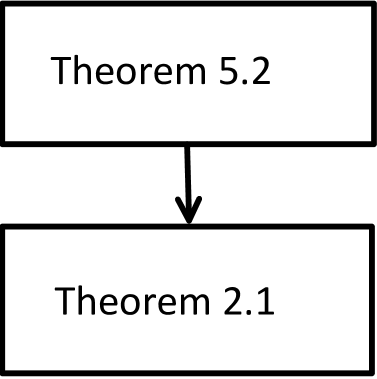
Figure 4. Theorem 2.1

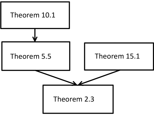
Figure 5. Theorem 2.3

3.1. Structure of the paper.

Figures 5 and 5 show the basic structure for proving the theorems that use the adjacency matrix. Recall that Theorem 2.1 is for Ising model, while Theorem 2.3 is for the Hard-core model.

Similarly, Figures 7 and 7 show the basic structure for proving the theorems that use the non-backtracking matrix.We have that Theorem 2.2 for Ising model, while Theorem 2.4 is for the Hard-core model. Note that Theorem 2.4 build on ideas that emerge in the proofs of both Theorems 2.3 and 2.2

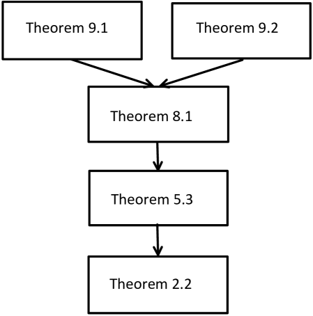
Figure 6. Theorem 2.2

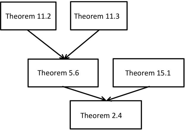
Figure 7. Theorem 2.4

4. Preliminaries

4.1. Measuring the speed of convergence for Markov Chains.

For measuring the distance between two distributions we use the notion of total variation distance. For two distributions $\upnu$ and $\hat{\upnu}$ on the discrete set $\Omega$, the total variation distance satisfies

$$||\upnu-\hat{\upnu}||_{tv} =(1/{2})\ {\sum\nolimits_{x\in\Omega}}|\upnu(x)-\hat{\upnu}(x)|\enspace.$$

We use the notion of mixing time as a measure for the rate that an ergodic Markov chain converges to equilibrium. More specifically, let be the transition matrix of an ergodic Markov chain ${\{X_{t}\}_{t\geq 0}}$ on a finite state space $\Omega$ with stationary distribution $\mu$. For $t\geq 0$ and $\sigma\in\Omega$, we let ${}^{t}(\sigma,\cdot)$ be the distribution of ${\{X_{t}\}_{t\geq 0}}$ when $X_{0}=\sigma$. Then, the mixing time of is defined by

$$T_{\rm mix}(\UpP)=\min\{t\geq 0\ :\ \forall\sigma\in\Omega\ \ ||{}^{t}(\sigma,\cdot)-\mu(\cdot)||_{tv}\leq 1/4\}\enspace.$$

4.2. Spectral Independence

We have seen the definition of the influence matrix before. However, since it is important to state the rapid mixing results we are using, we state it once more.

Consider a graph $G=(V,E)$. Assume that we are given a Gibbs distribution $\mu$ on the configuration space $\{\pm 1\}^{V}$. Then, for a given a set of vertices $\Lambda\subset V$ and a configuration $\tau$ at $\Lambda$, we let the pairwise influence matrix ${{\mathcal{I}}}^{\Lambda,\tau}_{G}$ be a matrix indexed by the vertices in $V\setminus\Lambda$ such that for any $v,w\in V\setminus\Lambda$, we have that

$${{\mathcal{I}}}^{\Lambda,\tau}_{G}(w,u) =\mu_{u}(+1\ |\ (\Lambda,\tau),(w,+1))-\mu_{u}(+1\ |\ (\Lambda,\tau),(w,-1))\enspace,$$ (4.1)

where $\mu_{u}(+1\ |\ (\Lambda,\tau),(w,+1))$ is the probability of the event that vertex $u$ has configuration $+1$, conditional on that the configuration at $\Lambda$ is $\tau$ and the configuration at $w$ is $+1$, We have the analogous for $\mu_{u}(+1\ |\ (\Lambda,\tau),(w,-1))$.

In the analysis we use the following folklore result which is standard to prove.

Claim 4.1.

For any graph $G=(V,E)$ and any Gibbs distribution $\mu:\{\pm 1\}^{V}\to[0,1]$ the following is true: For any $\Lambda\subseteq V$, for any $\tau\in\{\pm 1\}^{V}$, let be the $(V\setminus\Lambda)\times(V\setminus\Lambda)$ diagonal matrix such that for any $v\in V\setminus\Lambda$ we have that

$$\UpM(v,v) \textstyle=\sqrt{\mu^{\Lambda,\tau}_{v}(+1)\cdot\mu^{\Lambda,\tau}_{v}(-1)}\enspace.$$ (4.2)

Then, for ${{\mathcal{I}}}^{\Lambda,\tau}_{G}$ induced by $\mu$, the following is true: if is non-singular, the matrix ${}^{-1}\cdot{{\mathcal{I}}}^{\Lambda,\tau}_{G}\cdot\UpM$ is symmetric.

For the sake of our paper being self-contained, we provide a proof of Claim 4.1 in Section A.1.

Influence Matrix and Mixing Times

As far as the influence matrix ${{\mathcal{I}}}^{\Lambda,\tau}_{G}$ is concerned, the main focus is on $\theta_{1}({{\mathcal{I}}}^{\Lambda,\tau}_{G})$ i.e., the maximum eigenvalue.

Definition 4.2 (Spectral Independence).

For a real $\eta>0$, the Gibbs distribution $\mu_{G}$ on $G=(V,E)$ is $\eta$-spectrally independent, if for every $0\leq k\leq|V|-2$, $\Lambda\subseteq V$ of size $k$ and $\tau\in\{\pm 1\}^{\Lambda}$ we have that $\theta_{1}({\mathcal{I}}^{\Lambda,\tau}_{G})\leq 1+\eta$.

The notion of $\eta$-spectral independence for $\mu$ is related to (bounding) the mixing rate of the corresponding Glauber dynamics. One gets the following general result.

Theorem 4.3 ([3]).

For $\eta>0$, there is a constant $C\geq 0$ such that if $\mu$ is an $\eta$-spectrally independent distribution, then Glauber dynamics for sampling from $\mu$ has mixing time which is at least $Cn^{2+\eta}$.

Theorem 4.3 implies that for bounded $\eta$, the mixing time of Glauber dynamics is polynomial in $n$. However, this polynomial can be very large. There have been improvements on Theorem 4.3 since its introduction in [3], e.g., see [8, 12, 13].

For our results, we use a theorem from [12] which applies to graphs with bounded maximum degree ${\Delta}$.

First, before stating the theorem, we need to introduce a few useful concepts. For $S\subset V$, let the Hamming graph ${\tt Ham}_{S}$ be the graph whose vertices correspond to the configurations $\{\pm 1\}^{S}$, while two configurations are adjacent iff they differ at the assignment of a single vertex, i.e., their Hamming distance is one. Similarly, any subset $\Omega_{0}\subseteq\{\pm 1\}^{S}$ is considered to be connected if the subgraph induced by $\Omega_{0}$ is connected.

A distribution $\mu$ over $\{\pm 1\}^{V}$ is considered to be totally connected if for every nonempty $\Lambda\subset V$ and every boundary condition $\tau$ at $\Lambda$ the set of configurations in the support of $\mu(\cdot\ |\ \Lambda,\tau)$ is connected.

We remark here that all Gibbs distributions with soft-constraints such as the Ising model are totally connected in a trivial way. The same holds for the Hard-core model and this follows from standard arguments.

Definition 4.4.

For some number $b\geq 0$, we say that a distribution $\mu$ over $\{\pm 1\}^{V}$ is $b$-marginally bounded if for every $\Lambda\subset V$ and any configuration $\tau$ at $\Lambda$ we have the following: for any $V\setminus\Lambda$ and for any $x\in\{\pm 1\}$ which is in the support of $\mu_{u}(\cdot\ |\ \Lambda,\tau)$, we have that

$$\mu_{u}(x\ |\ \Lambda,\tau)\geq b\enspace.$$

The following result is a part of Theorem 1.9 from [12] (arxiv version).

Theorem 4.5 ([12]).

Let the integer ${\Delta}\geq 3$ and $b,\eta\in\mathbb{R}_{>0}$. Consider $G=(V,E)$ a graph with $n$ vertices and maximum degree ${\Delta}$. Also, let $\mu$ be a totally connected Gibbs distribution on $\{\pm 1\}^{V}$.

If $\mu$ is both $b$-marginally bounded and $\eta$-spectrally independent, then there are constants $C_{1},C_{2}>0$ such the Glauber dynamics for $\mu$ exhibits mixing time

$$T_{\rm mix} \leq\left({{\Delta}}/{b}\right)^{C_{1}\left(\frac{\eta}{b^{2}}+1\right)}\times C_{2}\left(n\log n\right)\enspace.$$

Theorem 4.5 implies $O(n\log n)$ mixing for provided that ${\Delta}$, $\eta$ and $\beta^{-1}$ are bounded, independent of $n$.

4.3. Basic Linear algebra

For a square $N\times N$ matrix , we let $\theta_{i}(\UpL)$, for $i\in[N]$ denote the eigenvalues of such that $\theta_{1}(\UpL)\geq\theta_{2}(\UpL)\geq\ldots\geq\theta_{N}(\UpL)$. Also, we let ${\Upphi}(\UpL)$ denote the set of distinct eigenvalues of . We also refer to ${\Upphi}(\UpL)$ as the spectrum of .

We define the spectral radius of , denoted as ${\rho}(\UpL)$, to be the real number such that

$${\rho}(\UpL)=\max\{|\theta|\ :\ \theta\in{\Upphi}(\UpL)\}\enspace.$$

It is a well-known result that the spectral radius of is the greatest lower bound for all of its matrix norms, e.g. see Theorem 6.5.9 in [27]. Letting $\left|\left|\cdot\right|\right|$ be a matrix norm on $N\times N$ matrices, we have that

$${\rho}(\UpL)\leq\left|\left|\UpL\right|\right|\enspace.$$ (4.3)

It is useful to mention that for the special case where is symmetric, i.e., $\UpL(i,j)=\UpL(j,i)$ for all $i,j\in[N]$, we have that ${\rho}(\UpL)=\left|\left|\UpL\right|\right|_{2}$.

For $\UpD,\UpB,\UpC\in\mathbb{R}^{N\times N}$, we let $|\UpD|$ denote the matrix having entries $|{}_{i,j}|$. For the matrices , we define $\UpB\leq\UpC$ to mean that ${}_{i,j}\leq{}_{i,j}$ for each $i$ and $j$. The following is a folklore result in linear algebra (e.g. see [33, 27]).

Lemma 4.6.

For integer $N>0$, let $\UpD,\UpB\in\mathbb{R}^{N\times N}$. If $|\UpD|\leq\UpB$, then ${\rho}(\UpD)\leq{\rho}(|\UpD|)\leq{\rho}(\UpB)$.

Concluding, for the matrix $\UpL\in\mathbb{R}^{N\times N}$ we follow the convention to call it non-negative, if all its entries are non-negative numbers, i.e., every entry ${}_{i,j}\geq 0$.

4.4. The adjacency matrix _G

For an undirected graph $G=(V,E)$ the adjacency matrix _G is a zero-one, $V\times V$ matrix such that for every pair $u,w\in V$ we have that

$${}_{G}(u,w)=\mathds{1}\{\textrm{ $u,w$ are adjacent in $G$}\}\enspace.$$

A natural property of the adjacency matrix is that for any two $u,w\in V$ and $\ell\geq 1$ we have that

$$\left({}^{\ell}_{G}\right)(u,w) =\textrm{$\#$ length $\ell$ walks\ from}\ u\ \textrm{to}\ w\enspace.$$ (4.4)

A walk in the graph $G$ is any sequence of vertices $w_{0},\ldots,w_{\ell}$ such that each consecutive pair $(w_{i-1},w_{i})$ is an edge in $G$. The length of the walk is equal to the number of consecutive pairs $(w_{i-1},w_{i})$.

Since we assume that the graph is undirected, we have that ${}^{\ell}_{G}$ is symmetric, for any integer $\ell\geq 0$. Hence, _G has real eigenvalues, while the eigenvectors corresponding to distinct eigenvalues are orthogonal with each other. We denote with ${\upphi}_{j}\in\mathbb{R}^{V}$ the eigenvector of _G that corresponds to the eigenvalue $\theta_{j}({}_{G})$, i.e., the $j$-th largest eigenvalue. Unless otherwise specified, we always take ${\upphi}_{j}$ such that $\textstyle\left|\left|{\upphi}_{j}\right|\right|_{2}=1$.

Our assumption that $G$ is always connected implies that _G is non-negative and irreducible. Hence, the Perron Frobenius Theorem (see appendix B ) implies that

$${\rho}({}_{G}) =\theta_{1}({}_{G}) \upphi_{1}(u) >0\qquad\forall u\in V\enspace.$$ and (4.5)

Note that if $G$ is bipartite, then we also have ${\rho}({}_{G})=|\theta_{n}({}_{G})|$.

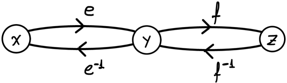
Figure 8. Oriented edges

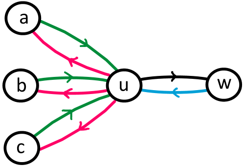
Figure 9. coloured edges

4.5. The Hashimoto non-backtracking matrix

Here we define the Hashimoto non-backtracking matrix, first introduced in [24].

For the graph $G=(V,E)$, let $M$ be the set of oriented edges obtained by doubling each edge of $E$ into two directed edges, i.e., one edge for each direction. The non-backtracking matrix, denoted as _G, is an $M\times M$, zero-one matrix such that for any pair of oriented edges $e=uw$ and $f=zy$ we have that

$${}_{G}(e,f)=\mathds{1}\{w=z\}\times\mathds{1}\{u\neq y\}\enspace.$$

That is, $\UpH(e,f)$ is equal to $1$, if $f$ follows the edge $e$ without creating a loop, otherwise, it is equal to zero. The reader is referred to the example in Fig. 9. For the edges $e,f$ in this example we have that ${}_{G}(e,f)=1$, we also have ${}_{G}(e^{-1},f^{-1})=1$. On the other hand, for ${}_{G}(e^{-1},f)=0$, etc.

As opposed to _G, the connectivity $G$ does not necessarily imply that _G is irreducible. It is a folklore result, e.g. also see [22], that _G is irreducible when $G$ is connected, the minimum degree ${\delta}(G)\geq 2$, but it is not a cycle.

Note that _G is not a symmetric matrix, i.e., ${}_{G}\neq\bar{\UpH}_{G}$. The assumption that it is irreducible, together with the Perron Frobenius Theorem, imply that the maximum eigenvalue is a positive real number (and algebraically simple).

PT-Invariance:

It was mentioned above that _G is not symmetric. In actuality _G is not normal, that is ${}_{G}\cdot\bar{\UpH}_{G}\neq\bar{\UpH}_{G}\cdot{}_{G}$. However, this matrix possesses a certain type of symmetry which, in mathematical physics, is called PT-invariance, where PT stands for parity-time. Formally, PT-invariance can be described as follows: for ${\bf x}\in\mathbb{R}^{M}$, the vector ${\bf x}^{\star}$ is such that

$${\bf x}^{\star}(e) ={\bf x}(e^{-1}) \forall e\in M\enspace,$$ (4.6)

where $e^{-1}$ is the edge that has the opposite direction to the edge $e\in M$. Furthermore, let be an involution on $\mathbb{R}^{M}$ such that

$$\UpP\cdot{\bf x}={\bf x}^{\star}\enspace.$$ (4.7)

Then, PT-Invariance for _G implies that for any integer $k\geq 0$, we have that

$${}^{k}_{G}\cdot\UpP =\UpP\cdot\bar{\UpH}^{k}_{G}\enspace.$$ (4.8)

The above implies that for any $e,f\in M$ and for any integer $k\geq 0$ we have that

$${}^{k}_{G}(e,f) ={}^{k}_{G}(f^{-1},e^{-1})\enspace.$$ (4.9)

The Eigenvectors:

Since we expect that _G is not normal, for the maximum eigenvalue we expect to have different left and right eigenvectors. Both of them arise in our analysis.

We let ${\upkappa}_{1}\in\mathbb{R}^{M}$ be the right principal eigenvector of _G, while let ${\uppsi}_{1}\in\mathbb{R}^{M}$ be the left principal eigenvector. An important observation for the two principal eigenvectors of _G is that $\UpP\cdot{\upkappa}_{1}={\uppsi}_{1}$. That is,

$${\upkappa}_{1}(e) ={\uppsi}_{1}(e^{-1}) \forall e\in M\enspace.$$ (4.10)

Furthermore, for any vertex $u\in V$ and any $w\in N_{G}(u)$ we have that

$$\sum_{v\in N_{G}(u):v\neq w}{\upkappa}_{1}(uv) =\theta_{1}\cdot{\upkappa}_{1}(wu) \sum_{v\in N_{G}(u):v\neq w}{\uppsi}_{1}(vu) =\theta_{1}\cdot{\uppsi}_{1}(uw)\enspace,$$ and (4.11)

i.e., since we work with oriented edges, we need to be cautious on the orientation of the indices of the eigenvector in the equation above.

To visualise the above, consider the example in Fig. 9. The sum of the component of ${\upkappa}_{1}$ that correspond to the red edges is equal to $\theta_{1}$ times the component that corresponds to the blue edge. On the other hand, for ${\uppsi}_{1}$, the sum of the components that correspond to the green edges is equal to $\theta_{1}$ times the component that corresponds to the black edge.

Assuming that _G is irreducible, the Perron Frobenius Theorem (see appendix B ) implies that then for $e\in M$ we have that

$${\uppsi}_{1}(e),\ {\upkappa}_{1}(e)>0\enspace.$$ (4.12)

Claim 4.7.

For $\uptheta>1$, consider the graph $G=(V,E)$ and assume that _G is irreducible and has spectral radius $\uptheta$. Suppose that there is an integer $L>0$, such that for each $e\in M$ there is $\ell\leq L$ such that ${}^{\ell}_{G}(e,e^{-1})>0$. Then, for all $e\in M$ we have that

$${\upkappa}_{1}(e^{-1})\leq\uptheta^{L-1}\cdot{\upkappa}_{1}(e)\enspace.$$ (4.13)

Proof.

Since _G is irreducible, (4.11) implies that for any $s,f\in M$ such that ${}_{G}(s,f)>0$ we have that

$${\upkappa}_{1}(f) \leq\uptheta\cdot{\upkappa}_{1}(s)\enspace.$$ (4.14)

Fix an edge $e\in M$. Our assumption is that there is at least one non-backtracking path $P$ from $e$ to $e^{-1}$ which is of length $\ell$ where $\ell\leq L$, i.e., since ${}^{\ell}_{G}(e,e^{-1})>0$.

Let $P=e_{1},e_{2},\ldots,e_{\ell}$ be a path connecting $e$ and $e^{-1}$, i.e., we have $e_{1}=e$ and $e_{\ell}=e^{-1}$. Since $P$ is non-backtracking, for any $1\leq i<\ell$ we have that ${}_{G}(e_{i},e_{i+1})=1$, while (4.14) implies that

$${\upkappa}_{1}(e_{i+1}) \leq\uptheta\cdot{\upkappa}_{1}(e_{i})\enspace.$$ (4.15)

Then, a simple induction implies that ${\upkappa}_{1}(e_{\ell})\leq\uptheta^{\ell-1}{\upkappa}_{1}(e_{1})$. Clearly, (4.13) follows, since $\ell\leq L$ and $e_{\ell}=e^{-1}$ and $e_{1}=e$.

This concludes the proof of Claim 4.7. ∎

5. Spectral Bounds for ${{\mathcal{I}}}^{\Lambda,\tau}_{G}$ using Tree Recursions

Consider the tree $T=(V_{T},E_{T})$, rooted at vertex $r$, while assume that every vertex has at most ${\Delta}$ children, for integer ${\Delta}>0$. Also, let $\mu$ be a Gibbs distribution on $\{\pm 1\}^{V_{T}}$, specified as in (2.1) with respect to the parameters $\beta,\gamma$ and $\lambda$.

For the region $K\subseteq V_{T}\setminus\{r\}$ and $\tau\in\{\pm 1\}^{K}$, let the ratio of marginals at the root ${R}^{K,\tau}_{r}$ be defined by

$${R}^{K,\tau}_{r}=\frac{\mu_{r}(+1\ |\ K,\tau)}{\mu_{r}(-1\ |\ K,\tau)}\enspace.$$ (5.1)

Recall that $\mu_{r}(\cdot\ |\ K,\tau)$ denotes the marginal of the Gibbs distribution $\mu(\cdot\ |\ K,\tau)$ at the root $r$. Also, note that the above allows for ${R}^{K,\tau}_{r}=\infty$, i.e., when $\mu_{r}(-1\ |\ K,\tau)=0$.

For a vertex $u\in V_{T}$, we let $T_{u}$ be the subtree of $T$ that includes $u$ and all its descendents. We always assume that the root of $T_{u}$ is the vertex $u$. With a slight abuse of notation, we let ${R}^{K,\tau}_{u}$ denote the ratio of marginals at the root for the subtree $T_{u}$, where the Gibbs distribution is, now, with respect to $T_{u}$, while we impose the boundary condition $\tau(K\cap T_{u})$.

Suppose that the vertices $w_{1},\ldots,w_{d}$ are the children of the root $r$, i.e., root is of degree $d>0$. It is standard to express ${R}^{K,\tau}_{r}$ in terms of ${R}^{K,\tau}_{w_{i}}$’s by having ${R}^{K,\tau}_{r}=F_{d}({R}^{K,\tau}_{w_{1}},{R}^{K,\tau}_{w_{2}},\ldots,{R}^{K,\tau}_{w_{d}})$, for

$$F_{d}:[0,+\infty]^{d}\to[0,+\infty] (x_{1},\ldots,x_{d})\mapsto\lambda\prod^{d}_{i=1}\frac{\beta{x}_{i}+1}{{x}_{i}+\gamma}\enspace.$$ such that (5.2)

In order to get cleaner results in the analysis, we work with log-ratios rather than ratios of Gibbs marginals. Let $H_{d}=\log\circ F_{d}\circ\exp$, which means that

$$H_{d}:[-\infty,+\infty]^{d}\to[-\infty,+\infty] \textstyle(x_{1},\ldots,x_{d})\mapsto\log\lambda+\sum^{d}_{i=1}\log\left(\frac{\beta\exp(x_{i})+1}{\exp(x_{i})+\gamma}\right)\enspace.$$ s.t. (5.3)

From (5.2), it is elementary to verify that $\log{R}^{K,\tau}_{r}=H_{d}(\log{R}^{K,\tau}_{w_{1}},\ldots,\log{R}^{K,\tau}_{w_{d}})$.

Finally, we let the function

$$h:[-\infty,+\infty]\to\mathbb{R} x\mapsto-\frac{(1-\beta\gamma)\cdot\exp(x)}{(\beta\exp(x)+1)(\exp(x)+\gamma)}\enspace.$$ s.t. (5.4)

It is straightforward that for $i\in[d]$, we have that $\frac{\partial}{\partial x_{i}}H_{d}(x_{1},\ldots,x_{d})=h(x_{i})$, where recall that $[d]=\{1,\ldots,d\}$. Furthermore, let the interval $J_{d}\subseteq\mathbb{R}$ be defined by

$$J_{d} =\left\{\begin{array}[]{lcl}[(\log\lambda\beta^{d}),\log(\lambda/\gamma^{d})]&&\textrm{if $\beta\gamma<1$}\enspace,\\ \vspace{-.3cm }\\ [(\log\lambda/\gamma^{d}),\log(\lambda\beta^{d})]&&\textrm{if $\beta\gamma>1$}\enspace.\end{array}\right.$$ (5.8)

Standard algebra implies that $J_{d}$ contains all the log-ratios for a vertex with $d$ children. Also, let

$$J =\textstyle\bigcup_{d\in[{\Delta}]}J_{d}\enspace.$$ (5.9)

The set $J$ contains all log-ratios in the tree $T$.

5.1. First attempt

Having introduced the notion of the (log-)ratio of Gibbs marginals and the related recursions we present the first set of our results that we use to establish spectral independence.

Definition 5.1 ($\delta$-contraction).

Let $\delta\geq 0$, the integer ${\Delta}\geq 1$ and $\beta,\gamma,\lambda\in\mathbb{R}$ are such that $0\leq\beta\leq\gamma$, $\gamma>0$ and $\lambda>0$. We say that the set of functions $\{H_{d}\}_{d\in[\Delta]}$, defined in (5.3), exhibits $\delta$-contraction, with respect to $(\beta,\gamma,\lambda)$, if it satisfies the following condition:

For any $d\in[{\Delta}]$ and every $({y}_{1},\ldots,{y}_{d})\in[-\infty,+\infty]^{d}$ we have that $||\nabla H_{d}({y}_{1},\ldots,{y}_{d})||_{\infty}\leq\delta.$

Clearly, the $\delta$-contraction condition is equivalent to having $h(z)\leq\delta$, for any $z\in[-\infty,+\infty]$, where $h(z)$ is defined in (5.4).

Theorem 5.2 (Adjacency Matrix).

Let ${\rho}\geq 1$, the integer ${\Delta}\geq 1$, $\varepsilon\in(0,1)$. Also, let $\beta,\gamma,\lambda\in\mathbb{R}$ be such that $0\leq\beta\leq\gamma$, $\gamma>0$ and $\lambda>0$.

Consider the graph $G=(V,E)$ of maximum degree ${\Delta}$, while the adjacency matrix _G is of spectral radius ${\rho}$. Also, consider $\mu$ the Gibbs distribution on $G$, specified by the parameters $(\beta,\gamma,\lambda)$.

For $\delta=\frac{1-\varepsilon}{{\rho}}$, suppose that the set of functions $\{H_{d}\}_{d\in[{\Delta}]}$ specified with respect to $(\beta,\gamma,\lambda)$ exhibits $\delta$-contraction. Then, for any $\Lambda\subset V$ and any $\tau\in\{\pm 1\}^{\Lambda}$, the pairwise influence matrix ${{\mathcal{I}}}^{\Lambda,\tau}_{G}$, induced by $\mu$, satisfies that

$$\textstyle{\rho}\left({{\mathcal{I}}}^{\Lambda,\tau}_{G}\right) \leq\varepsilon^{-1}\enspace.$$

The proof of Theorem 5.2 appears in Section 7.

Theorem 5.3 (Hashimoto Matrix).

Let the integer ${\Delta}\geq 1$, ${\hat{c}}>0$, $\uptheta\geq 1$, $\varepsilon\in(0,1)$. Also, let $\beta,\gamma,\lambda\in\mathbb{R}$ be such that $0\leq\beta\leq\gamma$, $\gamma>0$ and $\lambda>0$.

Consider the graph $G=(V,E)$ of maximum degree ${\Delta}$, while assume that the non-backtracking matrix ${}_{G}\in{\mathbb{H}}_{n,{\hat{c}}}$ and has spectral radius $\uptheta$. Also, consider $\mu$ the Gibbs distribution on $G$, specified by the parameters $(\beta,\gamma,\lambda)$.

For $\delta=\frac{1-\varepsilon}{\uptheta}$, suppose that the set of functions $\{H_{d}\}_{d\in[{\Delta}]}$ specified with respect to $(\beta,\gamma,\lambda)$ exhibits $\delta$-contraction. Then, for any $\Lambda\subset V$ and any $\tau\in\{\pm 1\}^{\Lambda}$, the pairwise influence matrix ${{\mathcal{I}}}^{\Lambda,\tau}_{G}$, induced by $\mu$, satisfies that

$$\textstyle{\rho}\left({{\mathcal{I}}}^{\Lambda,\tau}_{G}\right) \leq 1+{\hat{c}}\cdot{\Delta}/\varepsilon\enspace.$$

The proof of Theorem 5.3 appears in Section 8.

5.2. Second Attempt

Perhaps it is interesting to mention that using Theorem 5.2 and working as in the proof of Theorem 2.1 one retrieves the rapid mixing results for the Hard-core model in [25]. In order to get improved results for the Hard-core mode, we utilise potential functions, together with results from [36].

Let $\Sigma$ be the set of functions $F:[-\infty,+\infty]\to(-\infty,+\infty)$ which is differentiable and increasing.

Definition 5.4 ($(s,\delta,c)$-potential).

Let $s\geq 1$, allowing $s=\infty$, $\delta,c>0$ and let the integer ${\Delta}\geq 1$. Also, let $\beta,\gamma,\lambda\in\mathbb{R}$ be such that $0\leq\beta\leq\gamma$, $\gamma>0$ and $\lambda>0$.

Consider $\{H_{d}\}_{d\in[\Delta]}$, defined in (5.3) with respect to $(\beta,\gamma,\lambda)$. The function ${\Psi}\in\Sigma$, with image $S_{{\Psi}}$, is called $(s,\delta,c)$-potential if it satisfies the following two conditions:

Contraction:

For $d\in[{\Delta}]$, for $(\tilde{\bf y}_{1},\ldots,\tilde{\bf y}_{d})\in(S_{{\Psi}})^{d}$, and ${\bf m}=({\bf m}_{1},\ldots,{\bf m}_{d})\in\mathbb{R}^{d}_{\geq 0}$ we have that

$$\chi\left(H_{d}({\bf y}_{1},\ldots,{\bf y}_{d})\right)\cdot\sum^{d}_{j=1}\frac{\left|h\left({\bf y}_{j}\right)\right|}{\chi\left({\bf y}_{j}\right)}\cdot{\bf m}_{j}\leq\delta^{\frac{1}{s}}\cdot\left|\left|{\bf m}\right|\right|_{s}\enspace,$$ (5.10)

where $\chi={\Psi}^{\prime}$, ${\bf y}_{j}={\Psi}^{-1}(\tilde{\bf y}_{j})$, while $h(\cdot)$ is the function defined in (5.4).

Boundedness:

We have that

$$\max_{{\bf z}_{1},{\bf z}_{2}\in J}\left\{\chi({\bf z}_{1})\cdot\frac{|h({\bf z}_{2})|}{\chi({\bf z}_{2})}\right\} \leq c\enspace.$$ (5.11)

The notion of the $(s,\delta,c)$-potential function we have above, is a generalisation of the so-called “$(\alpha,c)$-potential function” that was introduced in [11]. Note that the notion of $(\alpha,c)$-potential function implies the use of the $\ell_{1}$-norm in the analysis. The setting we consider here is more general. The condition in (5.10), somehow, implies that we are using the $\ell_{r}$-norm, where $r$ is the Hölder conjugate of the parameter $s$ in the $(s,\delta,c)$-potential function.

Theorem 5.5 (Adjacency Matrix).

Let the integer ${\Delta}>1$, ${\rho}>1$, $s\geq 1$, allowing $s=\infty$, let $\varepsilon\in(0,1)$ and $\zeta>0$. Also, let $\beta,\gamma,\lambda\in\mathbb{R}$ be such that $\gamma>0$, $0\leq\beta\leq\gamma$ and $\lambda>0$.

Consider the graph $G=(V,E)$ of maximum degree ${\Delta}$, while the adjacency matrix _G is of spectral radius ${\rho}$. Consider, also, $\mu$ the Gibbs distribution on $G$ specified by the parameters $(\beta,\gamma,\lambda)$.

For $\delta=\frac{1-\varepsilon}{{\rho}_{G}}$ and $c=\frac{\zeta}{{\rho}}$, suppose that there is a $(s,\delta,c)$-potential function ${\Psi}$ with respect to $(\beta,\gamma,\lambda)$. Then, for any $\Lambda\subset V$, for any $\tau\in\{\pm 1\}^{\Lambda}$, the influence matrix ${{\mathcal{I}}}^{\Lambda,\tau}_{G}$, induced by $\mu$, satisfies that

$${\rho}\left({{\mathcal{I}}}^{\Lambda,\tau}_{G}\right) \leq 1+\zeta\cdot(1-(1-\varepsilon)^{s})^{-1}\cdot\left({{\Delta}}/{{\rho}}\right)^{1-({1}/{s})}\enspace.$$ (5.12)

The proof of Theorem 5.5 appears in Section 10.

Theorem 5.6 (Hashimoto Matrix).

Let ${\Delta}>1$, ${\hat{c}}>0$, $\uptheta>1$, $s\geq 1$, allowing $s=\infty$, let $\epsilon\in(0,1)$ and $\zeta>0$. Also, let $\beta,\gamma,\lambda\in\mathbb{R}$ be such that $\gamma>0$, $0\leq\beta\leq\gamma$ and $\lambda>0$.

Consider the graph $G=(V,E)$ of maximum degree ${\Delta}$, while assume that the non-backtracking matrix ${}_{G}\in{\mathbb{H}}_{|V|,{\hat{c}}}$ and has spectral radius $\uptheta$. Consider, also, $\mu$ the Gibbs distribution on $G$ specified by the parameters $(\beta,\gamma,\lambda)$, while assume that $(\beta,\gamma,\lambda)$ give rise to $\mu$ being $b$-marginally bounded, for $b>0$.

For $\delta=\frac{1-\epsilon}{\uptheta}$ and $c=\frac{\zeta}{\uptheta}$, suppose that there is a $(s,\delta,c)$-potential function ${\Psi}$ with respect to $(\beta,\gamma,\lambda)$. Then, for any $\Lambda\subset V$, for any $\tau\in\{\pm 1\}^{\Lambda}$, the influence matrix ${{\mathcal{I}}}^{\Lambda,\tau}_{G}$, induced by $\mu$, satisfies that

$$\textstyle{\rho}\left({{\mathcal{I}}}^{\Lambda,\tau}_{G}\right) \leq 1+b^{-6}\cdot\zeta\cdot{\hat{c}}\cdot(1-(1-\varepsilon)^{1/s})^{-1}\cdot{\Delta}/\uptheta\enspace.$$

The proof of Theorem 5.6 appears in Section 11

6. ${T_{\rm SAW}}$ Construction for ${{\mathcal{I}}}^{\Lambda,\tau}_{G}$

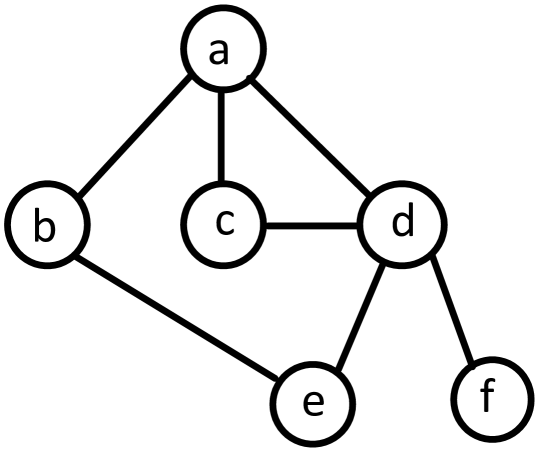
Figure 10. Initial graph $G$

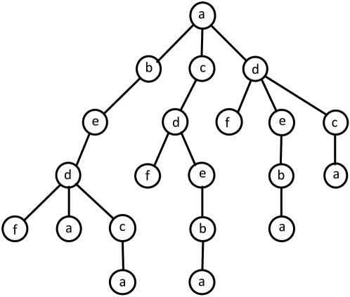
Figure 11. ${T_{\rm SAW}}(a)$

Consider the Gibbs distribution $\mu_{G}$ on the graph $G=(V,E)$, defined as in (2.1) with parameters $\beta,\gamma,\lambda\geq 0$. For $\Lambda\subseteq V$ and $\tau\in\{\pm\}^{\Lambda}$, recall the definition of the influence matrix ${{\mathcal{I}}}^{\Lambda,\tau}_{G}$ induced by $\mu$, from (4.1). Assume w.l.o.g. that there is a total ordering of the vertices in $V$, i.e., the vertex set of $G$.

We start by introducing the notion of the tree of self-avoiding walks in $G$. Recall that a walk is called self-avoiding if it does not repeat vertices. For each vertex $w$ in $G$, we define ${T_{\rm SAW}}(w)$, the tree of self-avoiding walks starting from $w$, as follows: Consider the set consisting of every walk $v_{0},\ldots,v_{r}$ in the graph $G$ that emanates from vertex $w$, i.e., $v_{0}=w$, while one of the following two holds

1. $v_{0},\ldots,v_{r}$ is a self-avoiding walk,

2. $v_{0},\ldots,v_{r-1}$ is a self-avoiding walk, while there is $j\leq r-3$ such that $v_{r}=v_{j}$.

Each one of the walks in the set corresponds to a vertex in ${T_{\rm SAW}}(w)$. Two vertices in ${T_{\rm SAW}}(w)$ are adjacent if the corresponding walks are adjacent. Two walks in graph $G$ are considered to be adjacent if one extends the other by one vertex .

For an example of the above construction, consider the graph $G$ in Fig. 11. In Fig. 11 we have the tree of self-avoiding walks that starts from vertex $a$ in $G$.

For the vertex in ${T_{\rm SAW}}(w)$ that corresponds to the walk $v_{0},\ldots,v_{r}$, we follow the convention to call it a “copy of vertex $v_{r}$”, i.e., $v_{r}$ is the last vertex in the path. Note that one vertex may have a lot of copies in ${T_{\rm SAW}}(w)$. For a vertex $v$ in $G$, we let ${\tt A}(v)$ be the set of its copies in ${T_{\rm SAW}}(w)$.

Consider the walk-tree $T={T_{\rm SAW}}(w)$. In what follows, we describe how the entry ${{\mathcal{I}}}^{\Lambda,\tau}_{G}(w,v)$ can be expressed using an appropriately defined spin-system on $T$. The exposition relies on results from [3, 11].

Let $\mu_{T}$ be a Gibbs distribution on $T$ which has the same specification as $\mu_{G}$. That is, for $\mu_{T}$ we use the same parameters $\beta,\gamma$ and $\lambda$ as those we have for $\mu_{G}$. Each $z\in{\tt A}(u)$ in the tree $T$, such that $u\in\Lambda$, is assigned a fixed configuration equal to $\tau(u)$. Furthermore, if we have a vertex $z$ in $T$ which corresponds to a path $w_{0},\ldots,w_{\ell}$ in $G$ such that $w_{\ell}=w_{j}$, for $0\leq j\leq\ell-3$, then we set a boundary condition at vertex $z$, as well. This boundary condition depends on the total ordering of the vertices. Particularly, we set at $z$

1. $-1$ if $w_{\ell}>w_{\ell-1}$,

2. $+1$ otherwise.

Let $\Gamma=\Gamma(G,\Lambda)$ be the set of vertices in $T$ which have a boundary condition in the above construction, while let $\sigma=\sigma(G,\tau)$ be the configuration we obtain at $\Gamma$.

For each $e$, edge in ${T_{\rm SAW}}(w)$, we specify weight $\upbeta(e)$ as follows: letting $e=\{x,z\}$ be such that $x$ is the parent of $z$ in ${T_{\rm SAW}}(w)$, we set

$$\upbeta(e)=\left\{\begin{array}[]{lcl}0&&\textrm{if there is boundary condition at either $x$, or $z$},\\ \textstyle h\left(\log{R}^{\Gamma,\sigma}_{z}\right)&&\textrm{otherwise}.\end{array}\right.$$ (6.3)

The function $h(\cdot)$ is from (5.4), while ${R}^{\Gamma,\sigma}_{z}$ is a ratio of Gibbs marginals at $z$ (see definitions in Section 5).

Then, we have the following proposition which is obtained from [3, 11].

Proposition 6.1 ([3, 11]).

For every $u,w\in V\setminus\Lambda$ we have that

$${{\mathcal{I}}}^{\Lambda,\tau}_{G}(w,v) =\sum\nolimits_{P}\prod\nolimits_{e\in P}\upbeta(e)\enspace,$$ (6.4)

where $P$ varies over all paths from the root of ${T_{\rm SAW}}(w)$ to the set of vertices in ${\tt A}(v)$.

7. Proof of Theorem 5.2

Recalling that $\delta=(1-\varepsilon)/{\rho}$, let be the $V\times V$ matrix defined by

$$=\sum^{n}_{\ell=0}\left(\delta\cdot{}_{G}\right)^{\ell}\enspace.$$ (7.1)

Since the adjacency matrix _G is symmetric, is symmetric, as well. It is direct that ${\rho}\left({{\UpB}}\right)\leq\epsilon^{-1}$, e.g.,

$${\rho}\left({{\UpB}}\right) =\left|\left|{{\UpB}}\right|\right|_{2}=\left|\left|\sum\nolimits_{\ell\geq 0}(\delta\cdot{}_{G})^{\ell}\right|\right|_{2}\leq\sum\nolimits_{\ell\geq 0}|\delta|^{\ell}\cdot\left|\left|({}_{G})^{\ell}\right|\right|_{2}\leq\sum\nolimits_{\ell\geq 0}(1-\varepsilon)^{\ell}=\varepsilon^{-1}\enspace.$$

Let _Λ by the principal submatrix of which is obtained by removing rows and columns that correspond to vertices in $\Lambda$. Cauchy’s interlacing theorem, e.g., see [27], implies that

$${\rho}\left({}_{\Lambda}\right) \leq{\rho}\left({{\UpB}}\right)\leq\varepsilon^{-1}\enspace.$$ (7.2)

We prove the theorem by showing that

$${\rho}\left({{\mathcal{I}}}^{\Lambda,\tau}_{G}\right) \leq{\rho}\left({}_{\Lambda}\right)\enspace.$$ (7.3)

In light of Lemma 4.6, we get (7.3) by showing that for any $u,w\in V\setminus\Lambda$ we have that

$$\left|{{\mathcal{I}}}^{\Lambda,\tau}_{G}(w,u)\right| \leq{}_{\Lambda}(w,u)\enspace.$$ (7.4)

It is immediate that for $u=w$ we have that $\left|{{\mathcal{I}}}^{\Lambda,\tau}_{G}(w,u)\right|=1$, while ${{\UpB}}(w,u)\geq 1$ as the summad in (7.1) for $\ell=0$ corresponds to the identity matrix. Fix $w,u\in V\setminus\Lambda$ such that $w\neq u$. Recall from the construction of Section 6 and Proposition 6.1 that

$${{\mathcal{I}}}^{\Lambda,\tau}_{G}(w,u) =\sum^{n}_{\ell=0}\sum_{P\in{\mathcal{P}}_{\ell}(u)}\prod_{e\in P}\upbeta(e)\enspace,$$ (7.5)

where the set ${\mathcal{P}}_{\ell}(u)$ consists of the paths of length $\ell$ that start from the root of ${T_{\rm SAW}}(w)$ and finish at a copy of vertex $u$ in the tree. Our assumption about $\delta$-contraction implies that for all edges $e$ in ${T_{\rm SAW}}(w)$, we have

$$\left|\upbeta(e)\right| \leq\delta\enspace.$$

Plugging the above into (7.5), we have that

$$\left|{{\mathcal{I}}}^{\Lambda,\tau}_{G}(w,u)\right| \leq\sum\nolimits_{\ell\geq 0}|{\mathcal{P}}_{\ell}(u)|\cdot\delta^{\ell}\enspace.$$ (7.6)

Let ${\rm SAW}_{\ell}(w,u)$ be the set of walks of length $\ell$ from $w$ to $u$, in the graph $G$, that correspond to the elements in ${\tt A}(u)$. Let ${\rm Walks}_{\ell}(w,u)$ be the set of walks of length $\ell$ from $w$ to $u$, in the graph $G$. We have that

$${\rm SAW}_{\ell}(w,u)\subseteq{\rm Walks}_{\ell}(w,u)\enspace,$$ (7.7)

since any element in ${\rm SAW}_{\ell}(w,u)$ is also a walk. It is standard that

$$|{\mathcal{P}}_{\ell}(u)| =|{\rm SAW}_{\ell}(w,u)|\leq|{\rm Walks}_{\ell}(w,u)|={}^{\ell}_{G}(w,u)\enspace.$$

The inequality above follows from (7.7), while the last equality is from (4.4).

Plugging the above bound into (7.6), we get that

$$\left|{{\mathcal{I}}}^{\Lambda,\tau}_{G}(w,u)\right| \leq\sum\nolimits_{\ell\geq 0}\delta^{\ell}\cdot{}^{\ell}(w,u)={}_{\Lambda}(w,u)\enspace.$$

The theorem follows by noting that the above implies (7.4) is true. $\Box$

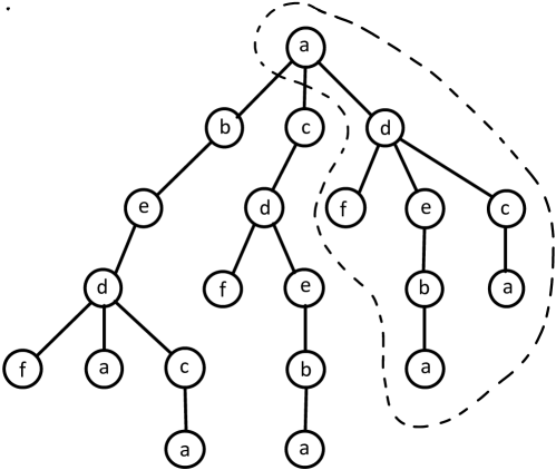
Figure 12. ${T_{\rm SAW}}(ad)$

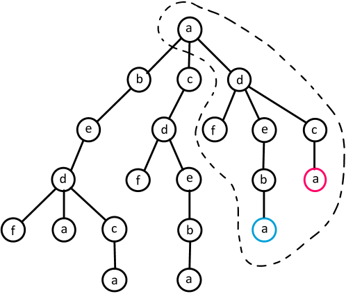
Figure 13. Copies of $ab$ and $ac$

8. Proof of Theorem 5.3

The proof of Theorem 5.3 is quite different from that of Theorem 5.2. Recall that for Theorem 5.2 we bound ${\rho}({{\mathcal{I}}}^{\Lambda,\tau}_{G})$ by just comparing the entries of ${{\mathcal{I}}}^{\Lambda,\tau}_{G}$ with the corresponding ones in _Λ. Theorem 5.3 follows by directly working with $\left|\left|{{\mathcal{I}}}^{\Lambda,\tau}_{G}\right|\right|_{2}$.

Before proving Theorem 5.3, we need to introduce a few concepts and some preliminary results.

8.1. A Refined norm bound

As in the standard setting for ${{\mathcal{I}}}^{\Lambda,\tau}_{G}$, consider the graph $G=(V,E)$, the Gibbs distribution $\mu$ on this graph, defined as in (2.1) with parameters $\beta,\gamma,\lambda\geq 0$. Also, let $\Lambda\subseteq V$ and $\tau\in\{\pm 1\}^{\Lambda}$.

Recall the set $M$ of oriented edges in $G$, that is

$$M=\{ws\ |\ w,s\in V\ \textrm{such that}\ s\neq w\ \textrm{and}\ {\{w,s\}\in E}\}\enspace.$$ (8.1)

We also let the set $M_{\Lambda}\subseteq M$ consists of all the elements $ws\in M$, such that $w,s\in V\setminus\Lambda$.

For $ws\in M$, we let $T_{{\rm SAW}}(ws)$ be the subtree of $T_{{\rm SAW}}(w)$ induced by the root of $T_{{\rm SAW}}(w)$, the child of the root which is a copy of vertex $s$, as well as the descendants of that copy. E.g., considering the tree of self-avoiding walks ${T_{\rm SAW}}(a)$ in Fig. 11, we have ${T_{\rm SAW}}(ad)$ in Fig. 13, i.e., the subtree that is enclosed within the dotted line.

For $uz\in M$, we say that vertex $v$ in $T_{{\rm SAW}}(ws)$ is a copy of $uz$ if $v$ is a copy of $u$ and, at the same time, the parent of $v$ is a copy of vertex $z$. E.g., in Fig. 13 the blue vertex is a copy of $ab$, while the red vertex is a copy of $ac$.

For integer $1\leq\ell\leq n$, for $\theta\in\mathbb{R}_{\geq 0}$, we define $\mathcal{E}^{\theta,\ell}_{\Lambda}$ to be the $M_{\Lambda}\times M_{\Lambda}$ matrix obtained as follows: for any $ws,uz\in M_{\Lambda}$ such that $w\neq u$, we have that

$$\mathcal{E}^{\theta,\ell}_{\Lambda}(ws,uz) =|{\tt C}(uz,\ell)|\cdot\theta^{\ell}\enspace,$$ (8.2)

where ${\tt C}(uz,\ell)$ is the set of copies of $uz$ in ${T_{\rm SAW}}(ws)$ that correspond to self-avoiding walks of length $\ell$ in graph $G$. Note that there might be copies of $uz$ in ${T_{\rm SAW}}(ws)$ that correspond to walks of length $\ell$ in $G$ which are not self-avoiding. These copies are not included in ${\tt C}(uz,\ell)$.

Furthermore, for any $ws,uz\in M_{\Lambda}$ such that $w=u$, we have that $\mathcal{E}^{\theta,\ell}_{\Lambda}(ws,uz)=0$.

Intuitively, under the $\delta$-contraction assumption, one could view the entry $\mathcal{E}^{\theta,\ell}_{\Lambda}(ws,uz)$ as an upper bound on the influence from $w$ to $u$ in $G$, “restricted” to the paths that start with edge $\{w,s\}$ and end with the edge $\{u,z\}$.

Theorem 8.1.

Let $\delta\in\mathbb{R}_{>0}$ and the integer ${\Delta}\geq 1$. Also, let $\beta,\gamma,\lambda\in\mathbb{R}$ be such that $0\leq\beta\leq\gamma$, $\gamma>0$ and $\lambda>0$. Consider the graph $G=(V,E)$ of maximum degree ${\Delta}$, while let $\mu$ be the Gibbs distribution on $G$ specified by the parameters $(\beta,\gamma,\lambda)$.

Suppose that the set of functions $\{H_{d}\}_{d\in[{\Delta}]}$ specified by $(\beta,\gamma,\lambda)$ exhibits $\delta$-contraction. Then, for any $\Lambda\subseteq V$, for any $\tau\in\{\pm 1\}^{\Lambda}$ and any $M_{\Lambda}\times M_{\Lambda}$ non-negative, non-singular, diagonal matrices _ℓ, where $1\leq\ell\leq n$, we have that

$$\left|\left|{{\mathcal{I}}}^{\Lambda,\tau}_{G}\right|\right|_{2} \leq 1+{\Delta}\cdot\sum\nolimits_{\ell\geq 1}\left|\left|{}^{-1}_{\ell}\cdot\mathcal{E}^{\delta,\ell}_{\Lambda}\cdot{}_{\ell}\right|\right|_{\infty}\enspace,$$ (8.3)

where ${{\mathcal{I}}}^{\Lambda,\tau}_{G}$ is specified with respect to $\mu$.

The proof of Theorem 8.1 appears in Section 9.

Note that Theorem 5.3 follows Theorem 8.1 by choosing appropriately the matrices _ℓ.

8.2. Proof of Theorem 5.3

Let ${\upkappa}_{1}$ be the right principal eigenvector of _G. Recall that ${\upkappa}_{1}$ is indexed by $M$, i.e., the set of oriented edges of $G$.

Since we have assumed that _G is irreducible, i.e., we have ${}_{G}\in{\mathbb{H}}_{n,{\hat{c}}}$, then we have that

$${\upkappa}_{1}(xv) >0 \forall xv\in M\enspace.$$ (8.4)

Let $\Upphi$ be the $M_{\Lambda}\times M_{\Lambda}$ diagonal matrix such that for any $xv\in M_{\Lambda}$ we have that

$$\Upphi(xv,xv) ={\upkappa}_{1}(vx)\enspace.$$ (8.5)

One needs to be cautious about the direction of the edge in the component of ${\upkappa}_{1}$ for the diagonal entries of $\Upphi$. Further note that, due to (8.4), the diagonal entries of $\Upphi$ are all positive, hence the matrix is non-singular.

Applying Theorem 8.1, where we set ${}_{\ell}=\Upphi$ for all $1\leq\ell\leq n$, we get that

$$\left|\left|{{\mathcal{I}}}^{\Lambda,\tau}_{G}\right|\right|_{2} \leq\ 1+{\Delta}\cdot\sum\nolimits_{\ell\in[n]}\left|\left|\Upphi^{-1}\cdot\mathcal{E}^{\delta,\ell}_{\Lambda}\cdot\Upphi\right|\right|_{\infty}\enspace,$$

where $\delta=\frac{1-\varepsilon}{\uptheta}$. In light of the above equality, the theorem follows by showing that

$$\left|\left|\Upphi^{-1}\cdot\mathcal{E}^{\delta,\ell}_{\Lambda}\cdot\Upphi\right|\right|_{\infty} \leq{\hat{c}}\cdot(1-\varepsilon)^{\ell} 1\leq\ell\leq n\enspace.$$ (8.6)

Fix $ws\in M_{\Lambda}$ and let

$${\mathcal{Q}}^{(\ell)}_{ws} =\sum\nolimits_{uz\in M_{\Lambda}}\left(\Upphi^{-1}\cdot\mathcal{E}^{\delta,\ell}_{\Lambda}\cdot\Upphi\right)(ws,uz)\enspace.$$

${\mathcal{Q}}^{(\ell)}_{ws}$ is nothing more than the absolute row sum for the row that corresponds to $ws$ in the matrix $\Upphi^{-1}\cdot\mathcal{E}^{\delta,\ell}_{\Lambda}\cdot\Upphi$. We don’t need to use absolute values here since the matrices are non-negative.

Clearly, (8.6) follows by proving that, regardless of the choice of $ws$, we have

$${\mathcal{Q}}^{(\ell)}_{ws} \leq{\hat{c}}\cdot(1-\varepsilon)^{\ell} 1\leq\ell\leq n\enspace.$$ (8.7)

Let $T=T_{{\rm SAW}}(ws)$. Consider the vertex $v$ in the tree $T$, at level $0\leq h\leq\ell$. Also, recall that $T_{v}$ is the subtree that contains $v$ and all its descendants. Let ${{\mathcal{R}}}_{v}$ be defined by

$${\mathcal{R}}_{v} =\sum\nolimits_{uz\in M_{\Lambda}}\frac{\Upphi(uz,uz)}{\Upphi(ws,ws)}\cdot|{\tt C}(uz,\ell)\cap T_{v}|\cdot\delta^{\ell-h}\enspace,$$

where, recall that, ${\tt C}(uz,\ell)$ is the set of copies of $uz$ in ${T_{\rm SAW}}(ws)$ that correspond to self-avoiding walks of length $\ell$ in $G$. With a slight abuse of notation, we use ${\tt C}(uz,\ell)\cap T_{v}$ to specify the elements of ${\tt C}(uz,\ell)$ that are also in the subtree $T_{v}$.

For a vertex $v\in T$ at level $h=\ell$, the above can be written as follows

$${\mathcal{R}}_{v}=\sum\nolimits_{uz\in M_{\Lambda}}\frac{\Upphi(uz,uz)}{\Upphi(ws,ws)}\cdot\mathds{1}\{v\in{\tt C}(uz,\ell)\}\enspace.$$ (8.8)

If vertex $v$ corresponds to the root of $T$, then the definition of matrix $\mathcal{E}^{\delta,\ell}_{\Lambda}$ implies that

$${\mathcal{R}}_{v}={\mathcal{Q}}^{(\ell)}_{ws}\enspace.$$ (8.9)

Hence, we prove (8.7) by showing that for any $0\leq h<\ell$, for any vertex $v$ at level $h$ in the tree $T$ which is a copy of $xq\in M$ (i.e., $v$ is a copy of $x$ with parent vertex being a copy of $q$), we have that

$${\mathcal{R}}_{v}\leq\frac{\Upphi(xq,xq)}{\Upphi(ws,ws)}\cdot(1-\varepsilon)^{\ell-h}=\frac{{\upkappa}_{1}(qx)}{{\upkappa}_{1}(sw)}\cdot(1-\varepsilon)^{\ell-h}\enspace.$$ (8.10)

For $h=0$, the above, together with (8.9) imply (8.7), since we have $qx=ws$ and $\frac{{\upkappa}_{1}(ws)}{{\upkappa}_{1}(sw)}\leq{\hat{c}}$ due to our assumption that ${}_{G}\in{\mathbb{H}}_{n,{\hat{c}}}$

We use mathematical induction to prove (8.10). The induction is on the quantity $\ell-h$. In our induction we use the following, elementary to show, observation: for a vertex $v$ at level $0\leq h<\ell$, whose children in $T_{v}$ are the vertices $v_{1},\ldots,v_{d}$, we have that

$${\mathcal{R}}_{v} =\delta\cdot\sum\nolimits_{v_{i}}{\mathcal{R}}_{v_{i}}\enspace.$$ (8.11)

We now proceed with the induction. The base corresponds to $\ell-h=1$. Then, from (8.11) we have that

$${\mathcal{R}}_{v} =\delta\cdot\sum\nolimits_{v_{i}}{\mathcal{R}}_{v_{i}}=\delta\cdot\sum\nolimits_{v_{i}}\sum\nolimits_{uz\in M_{\Lambda}}\frac{\Upphi(uz,uz)}{\Upphi(ws,ws)}\cdot\mathds{1}\{v_{i}\in{\tt C}(uz,\ell)\}\enspace.$$

The second equation is from (8.8), i.e., since it assumed that $\ell-h=1$, then $v_{i}$’s are at level $\ell$ of $T$. Suppose that $v_{i}$ is a copy of $q_{i}x\in M$ (Recall that $v$ is assumed to be a copy of $xq$.) Then, the above can be written as follows:

$${\mathcal{R}}_{v} =\delta\cdot\sum\nolimits_{q_{i}x}\frac{\Upphi(q_{i}x,q_{i}x)}{\Upphi(ws,ws)}=\delta\cdot\sum\nolimits_{xq_{i}}\frac{{\upkappa}_{1}(xq_{i})}{{\upkappa}_{1}(sw)}\enspace,$$ (8.12)

where in the second equality we use the definition of the matrix $\Upphi$. From (4.11), we further have that

$$\sum\nolimits_{q_{i}x}{\upkappa}_{1}(xq_{i}) \leq\uptheta\cdot{\upkappa}_{1}(qx)\enspace.$$ (8.13)

Plugging the above into (8.12), we get that

$${\mathcal{R}}_{v} \leq\delta\cdot\uptheta\cdot\frac{{\upkappa}_{1}(qx)}{{\upkappa}_{1}(sw)}=\frac{{\upkappa}_{1}(qx)}{{\upkappa}_{1}(sw)}(1-\epsilon)\enspace.$$

The last equality follows since $\delta=\frac{1-\varepsilon}{\uptheta}$. All the above conclude the proof of the base of the induction.

Suppose that (8.10) is true for some $\ell-h\geq 1$. We show that this hypothesis implies that the equation is true for $\ell-h+1$. As before, from (8.11) we have that

$${\mathcal{R}}_{v} =\delta\cdot\sum\nolimits_{v_{i}}{\mathcal{R}}_{v_{i}}\leq\delta\cdot\sum\nolimits_{q_{i}x}\frac{{\upkappa}_{1}(xq_{i})}{{\upkappa}_{1}(sw)}(1-\varepsilon)^{\ell-h}\enspace.$$

The last inequality is due to the induction hypothesis. Plugging (8.13) into the above inequality, we get that

$${\mathcal{R}}_{v}\leq\delta\cdot\uptheta\cdot\frac{{\upkappa}_{1}(qx)}{{\upkappa}_{1}(sw)}(1-\varepsilon)^{\ell-h}=\frac{{\upkappa}_{1}(qx)}{{\upkappa}_{1}(sw)}(1-\varepsilon)^{\ell-h+1}\enspace.$$

For the last equality we use, once again, that $\delta=\frac{1-\varepsilon}{\uptheta}$. This concludes the induction, hence (8.10) is true.

Theorem 5.3 follow. $\Box$

9. Proof of Theorem 8.1

9.1. Proof of Theorem 8.1

As in the standard setting for ${{\mathcal{I}}}^{\Lambda,\tau}_{G}$, consider the graph $G=(V,E)$ and the Gibbs distribution $\mu$ on $G$, defined as in (2.1) with parameters $\beta,\gamma,\lambda\geq 0$. Also, let $\Lambda\subseteq V$ and $\tau\in\{\pm 1\}^{\Lambda}$.

Recall that for the oriented edge $ws\in M$, we let $T_{{\rm SAW}}(ws)$ be the subtree of $T_{{\rm SAW}}(w)$ induced by the root of $T_{{\rm SAW}}(w)$, the child of the root which is a copy of vertex $s\in V$, as well as the descendants of that copy (see example in Fig. 13).

For $T_{{\rm SAW}}(w)$ consider the weights $\{\upbeta(e)\}_{e}$ as these are specified in (6.3) with respect to the Gibbs distribution $\mu^{\Lambda,\tau}$. We apply the same weights to the edges of $T_{{\rm SAW}}(ws)$. Since $T_{{\rm SAW}}(ws)$ is a subtree of $T_{{\rm SAW}}(w)$ this can be done in the standard way.

Consider now ${T_{\rm SAW}}(ws)$ with weights $\{\upbeta(e)\}_{e}$ at its edges. For $\ell\geq 1$, we let $\mathcal{S}_{\ell}=\mathcal{S}_{\ell}(G,\Lambda,\tau)$ be the $M_{\Lambda}\times M_{\Lambda}$ matrix defined such that for $ws,uz\in M_{\Lambda}$ with $w\neq u$, we have

$$\mathcal{S}_{\ell}(ws,uz) =\sum\nolimits_{P}\prod\nolimits_{e\in P}\upbeta(e)\enspace,$$ (9.1)

where $P$ varies over the paths from the root of ${T_{\rm SAW}}(ws)$ to the vertices in ${\tt C}(uz,\ell)$, while recall that ${\tt C}(uz,\ell)$ is the set of copies of $uz$ in $T$ that correspond to self-avoiding walks of length $\ell$ in $G$.

For any $ws,uz$ such that $u=w$ we have $\mathcal{S}_{\ell}(ws,uz)=0$.

Theorem 9.1.

Let $\delta\in\mathbb{R}_{\geq 0}$ and the integer ${\Delta}\geq 1$. Also, let $\beta,\gamma,\lambda\in\mathbb{R}$ be such that $0\leq\beta\leq\gamma$, $\gamma>0$ and $\lambda>0$. Consider the graph $G=(V,E)$ of maximum degree ${\Delta}$, while let $\mu$ be the Gibbs distribution on $G$ specified by the parameters $(\beta,\gamma,\lambda)$.

For any $\Lambda\subseteq V$, for any $\tau\in\{\pm 1\}^{\Lambda}$, for any non-singular matrices $\Upgamma_{\ell}$, where $1\leq\ell\leq n$, such that $\Upgamma_{\ell}$ and $\mathcal{S}_{\ell}$ are conformable for multiplication, we have that

$$\left|\left|{{\mathcal{I}}}^{\Lambda,\tau}_{G}\right|\right|_{2} \leq 1+{\Delta}\cdot\sum\nolimits_{\ell\geq 1}{}_{\ell}\enspace,$$

where ${}_{\ell}=\max\left\{\left|\left|\Upgamma_{\ell}^{-1}\cdot\mathcal{S}_{\ell}\cdot\Upgamma_{\ell}\right|\right|_{\infty},\ \left|\left|\Upgamma_{\ell}^{-1}\cdot\bar{\mathcal{S}}_{\ell}\cdot\Upgamma_{\ell}\right|\right|_{\infty}\right\}$ and $\bar{\mathcal{S}}_{\ell}$ is the transpose of $\mathcal{S}_{\ell}$.

The proof of Theorem 9.1 appears in Section 9.2.

Theorem 9.2.

Let $\delta\in\mathbb{R}_{\geq 0}$ and the integer ${\Delta}\geq 1$. Also, let $\beta,\gamma,\lambda\in\mathbb{R}$ be such that $0\leq\beta\leq\gamma$, $\gamma>0$ and $\lambda>0$. Consider the graph $G=(V,E)$ of maximum degree ${\Delta}$, while let $\mu$ be the Gibbs distribution on $G$ specified by the parameters $(\beta,\gamma,\lambda)$.

Suppose that the set of functions $\{H_{d}\}_{d\in[{\Delta}]}$ specified with respect to $(\beta,\gamma,\lambda)$ exhibits $\delta$-contraction. For any $\Lambda\subseteq V$, $\tau\in\{\pm 1\}^{\Lambda}$, for $1\leq\ell\leq n$ and any $M_{\Lambda}\times M_{\Lambda}$ non-singular, non-negative, diagonal matrix _ℓ we have that

$$\left|\left|{}^{-1}_{\ell}\cdot\mathcal{S}_{\ell}\cdot{}_{\ell}\right|\right|_{\infty} \leq\textstyle\left|\left|{}^{-1}_{\ell}\cdot\mathcal{E}^{\delta,\ell}_{\Lambda}\cdot{}_{\ell}\right|\right|_{\infty}\enspace.$$ (9.2)

The above inequality holds even when we replace the matrix $\mathcal{S}_{\ell}$ with its transpose $\bar{\mathcal{S}}_{\ell}$.

The proof of Theorem 9.2 appears in Section 9.3.

Clearly, Theorem 9.2 implies that the quantities _ℓ defined in Theorem 9.1 satisfy that

_ℓ $$\leq\left|\left|{}^{-1}_{\ell}\cdot\mathcal{E}^{\delta,\ell}_{\Lambda}\cdot{}_{\ell}\right|\right|_{\infty} 1\leq\ell\leq n\enspace.$$

From the above and Theorem 9.1 it is immediate to get (8.3).

Theorem 8.1 follows. $\Box$

9.2. Proof of Theorem 9.1

Fix $ws\in M_{\Lambda}$. For $T_{{\rm SAW}}(w)$ consider the weights $\{\upbeta(e)\}_{e}$ as these are specified in (6.3) with respect to the Gibbs distribution $\mu^{\Lambda,\tau}$. We apply the same weights to the edges of $T_{{\rm SAW}}(ws)$. Since $T_{{\rm SAW}}(ws)$ is a subtree of $T_{{\rm SAW}}(w)$ this can be done in the standard way.

We let $\mathcal{J}=\mathcal{J}(G,\Lambda,\tau)$ be an $M_{\Lambda}\times M_{\Lambda}$ matrix with entries in the interval $[-1,1]$. For every $ws,uz\in M_{\Lambda}$ such that $w\neq u$, the entry $\mathcal{J}^{\Lambda,\tau}_{G}(ws,uz)$ is defined by

$$\mathcal{J}(ws,uz) =\sum\nolimits_{P}\prod\nolimits_{e\in P}\upbeta(e)\enspace,$$ (9.3)

where $P$ varies over the paths from the root of ${T_{\rm SAW}}(ws)$ to the set of copies of $uz$ in this tree. Furthermore, for $ws,uz\in M_{\Lambda}$ such that $w=u$, we let $\mathcal{J}^{\Lambda,\tau}_{G}(ws,uz)=0$.

From the definitions of $\mathcal{J}$ and $\mathcal{S}$ it is not hard to see that

$$\mathcal{J} =\sum\nolimits_{\ell\geq 1}\mathcal{S}_{\ell}\enspace.$$

Also, it is standard to get matrices and such that

$${{\mathcal{I}}}^{\Lambda,\tau}_{G} =\UpI+\UpK\cdot\mathcal{J}\cdot\UpC\enspace,$$ (9.4)

where is the $(V\setminus\Lambda)\times(V\setminus\Lambda)$ identity matrix. Specifically, for and we have the following: is a $(V\setminus\Lambda)\times M_{\Lambda}$, zero-one matrix such that for any $r\in V\setminus\Lambda$ and any $vx\in M_{\Lambda}$ we have

$$\UpK(r,vx) =\mathds{1}\{r=v\}\enspace.$$ (9.5)

is a $M_{\Lambda}\times(V\setminus\Lambda)$ zero-one matrix, such that for any $r\in V\setminus\Lambda$ and any $xv\in M_{\Lambda}$ we have

$$\UpC(xv,r) =\mathds{1}\{x=r\}\enspace.$$ (9.6)

To see why (9.4) is true, e.g., we note that the definition of the matrices ${{\mathcal{I}}}^{\Lambda,\tau}_{G}$ and $\mathcal{J}$ imply that for any $u,w\in V\setminus\Lambda$ different with each other, we have that

$${{\mathcal{I}}}^{\Lambda,\tau}_{G}(w,u) =\sum_{vs\in M_{\Lambda}}\sum_{rz\in M_{\Lambda}}\mathds{1}\{v=w\}\cdot\mathds{1}\{r=u\}\cdot\mathcal{J}(vs,rz)\enspace.$$ (9.7)

It is elementary to verify that the entry $(\UpK\cdot\mathcal{J}\cdot\UpC)(w,u)$ is equal to the r.h.s. of the above equation.

Consider the block, anti-diagonal matrix defined by

$$=\left[\begin{array}[]{cc}{\bf 0}&{{\mathcal{I}}}^{\Lambda,\tau}_{G}\\ \textstyle\bar{{{\mathcal{I}}}}^{\Lambda,\tau}_{G}&{\bf 0}\end{array}\right]\enspace,$$ (9.10)

where $\bar{{{\mathcal{I}}}}^{\Lambda,\tau}_{G}$ is the transpose of ${{\mathcal{I}}}^{\Lambda,\tau}_{G}$ and ${\bf 0}$ is the zero matrix

Claim 9.3.

We have that $\left|\left|{{\mathcal{I}}}^{\Lambda,\tau}_{G}\right|\right|_{2}=\left|\left|\UpW\right|\right|_{2}$.

The above claim is standard. We provide a proof in Section A.2. In light of Claim 9.3, it suffices to prove that

$$\left|\left|\UpW\right|\right|_{2} \leq 1+{\Delta}\cdot\sum\nolimits_{\ell\geq 1}{}_{\ell}\enspace,$$ (9.11)

where _ℓ’s are defined in the statement of Theorem 9.1. Consider further the block matrices

$$=\left[\begin{array}[]{cc}{\bf 0}&\mathcal{J}\\ \bar{\mathcal{J}}&{\bf 0}\end{array}\right], =\left[\begin{array}[]{cc}\UpK\hfil&{\bf 0}\\ {\bf 0}&\bar{\UpC}\end{array}\right]\enspace,$$ (9.16)

where $\bar{\mathcal{J}},\bar{\UpC}$ correspond to the transpose of matrices $\mathcal{J}$ and , respectively.

From (9.4), (9.10) and straightforward calculations, we get that

$$=\UpJ+\UpT\cdot\UpY\cdot\bar{\UpT}\enspace,$$

where is the block anti-diagonal matrix, while the non-zero blocks are both the $(V\setminus\Lambda)\times(V\setminus\Lambda)$ identity matrix. Furthermore, we have that

$$\left|\left|\UpW\right|\right|_{2} =\left|\left|\UpJ+\UpT\cdot\UpY\cdot\bar{\UpT}\right|\right|_{2}\ \leq\left|\left|\UpJ\right|\right|_{2}+\left|\left|\UpT\right|\right|_{2}\cdot\left|\left|\UpY\right|\right|_{2}\cdot\left|\left|\bar{\UpT}\right|\right|_{2}$$

$$=1+\left|\left|\UpT\right|\right|^{2}_{2}\cdot\left|\left|\UpY\right|\right|_{2}\enspace.$$ (9.17)

The last derivation follows from the observation that $\left|\left|\UpJ\right|\right|_{2}=1$. Then, (9.11) follows by bounding appropriately the quantities on the r.h.s. of (9.17).

As far as $\left|\left|\UpT\right|\right|_{2}$ is concerned, we have the following result.

Claim 9.4.

We have that $\left|\left|\UpT\right|\right|_{2}\leq\sqrt{{\Delta}}$.

Proof.

Since is block-diagonal matrix, e.g., see (9.16), we work as in Claim 9.3 to get that

$$\left|\left|\UpT\right|\right|_{2} \leq\max\left\{\left|\left|\UpK\right|\right|_{2},\left|\left|\bar{\UpC}\right|\right|_{2}\right\}\enspace.$$

The claim follows by showing that both $\left|\left|\bar{\UpC}\right|\right|_{2},\left|\left|\UpK\right|\right|_{2}$ are at most $\sqrt{{\Delta}}$.

We start with . Consider the product $\UpK\cdot\bar{\UpK}$, where $\bar{\UpK}$ is the transpose. Note that $\UpK\cdot\bar{\UpK}$ is a $(V\setminus\Lambda)\times(V\setminus\Lambda)$ matrix. Furthermore, for any $u,w\in V\setminus\Lambda$ we have that

$$\left(\UpK\cdot\bar{\UpK}\right)(u,w) =\sum_{rx\in M_{\Lambda}}\UpK(u,rx)\cdot\bar{\UpK}(rx,w)$$

$$=\sum_{rx\in M_{\Lambda}}\mathds{1}\{u=r\}\times\mathds{1}\{w=r\}$$

$$=\mathds{1}\{w=u\}\times\sum_{rx\in M_{\Lambda}}\mathds{1}\{w=r\}$$

$$\leq\mathds{1}\{w=u\}\times{\rm deg}_{G}(w)\enspace,$$

the last inequality follows from the observation that having $rx\in M_{\Lambda}$ implies that $\{r,x\}\in E$. Hence, we conclude that $(\UpK\cdot\bar{\UpK})$ is a diagonal matrix, while $(\UpK\cdot\bar{\UpK})(w,w)\leq{\rm deg}(w)$. Clearly, we have that $\left|\left|\UpK\cdot{}^{*}\right|\right|_{2}\leq{\Delta}$ which implies that $\left|\left|\UpK\right|\right|_{2}\leq\sqrt{{\Delta}}$. Working similarly, we get the same bound for $\left|\left|\bar{\UpC}\right|\right|_{2}$.

The claim follows. ∎

As far as $\left|\left|\UpY\right|\right|_{2}$ is concerned, we work as follows: For $1\leq\ell\leq n$, let the block-matrix _ℓ be defined by

_ℓ $$=\left[\begin{array}[]{cc}{\bf 0}&\mathcal{S}_{\ell}\\ \bar{\mathcal{S}}_{\ell}&{\bf 0}\end{array}\right]\enspace.$$ (9.20)

Noting that $\UpY=\sum_{\ell\geq 1}{}_{\ell}$, we have that

$$\left|\left|\UpY\right|\right|_{2} \leq\sum\nolimits_{\ell\geq 1}\left|\left|{}_{\ell}\right|\right|_{2}\enspace.$$ (9.21)

It is easy to check that the matrix _ℓ, for $1\leq\ell\leq n$, is symmetric. Hence, we have that

$$\left|\left|{}_{\ell}\right|\right|_{2}\leq\left|\left|{}^{-1}_{\ell}\cdot\UpY\cdot{}_{\ell}\right|\right|_{\infty}\enspace,$$ (9.22)

for any non-singular matrix _ℓ such that _ℓ and _ℓ are conformable for multiplication. The above holds, since, for any normal matrix (hence also for _ℓ) we have that ${\rho}(\UpA)=\left|\left|\UpA\right|\right|_{2}\leq\left|\left|\UpA\right|\right|$  for any matrix norm $\left|\left|\cdot\right|\right|$. We choose _ℓ such that

_ℓ $$=\left[\begin{array}[]{cc}{\bf 0}&\Upgamma_{\ell}\\ \Upgamma_{\ell}&{\bf 0}\end{array}\right] {}^{-1}_{\ell} =\left[\begin{array}[]{cc}{\bf 0}&\Upgamma^{-1}_{\ell}\\ \Upgamma^{-1}_{\ell}&{\bf 0}\end{array}\right]\enspace,$$ and (9.27)

where matrix $\Upgamma_{\ell}$ is from the statement of Theorem 9.1. Since $\Upgamma_{\ell}$ is assumed to be non-singular, it is straightforward that ${}^{-1}_{\ell}$ is well defined.

Furthermore, from the definition of the matrices _ℓ and _ℓ, we have that

$${}^{-1}_{\ell}\cdot{}_{\ell}\cdot{}_{\ell} =\left[\begin{array}[]{cc}{\bf 0}&\Upgamma^{-1}_{\ell}\cdot\bar{\mathcal{S}}_{\ell}\cdot\Upgamma_{\ell}\\ \Upgamma^{-1}_{\ell}\cdot\mathcal{S}_{\ell}\cdot\Upgamma_{\ell}&{\bf 0}\end{array}\right]\enspace.$$ (9.30)

Note that the matrix ${}^{-1}_{\ell}\cdot{}_{\ell}\cdot{}_{\ell}$ is not necessarily symmetric. However, it is standard that

$$\left|\left|{}^{-1}_{\ell}\cdot{}_{\ell}\cdot{}_{\ell}\right|\right|_{\infty} \leq\max\left\{\left|\left|\Upgamma^{-1}_{\ell}\cdot\mathcal{S}_{\ell}\cdot\Upgamma_{\ell}\right|\right|_{\infty},\ \left|\left|\Upgamma^{-1}_{\ell}\cdot\bar{\mathcal{J}}_{\ell}\cdot\Upgamma_{\ell}\right|\right|_{\infty}\right\}={}_{\ell}\enspace.$$

From the above, (9.21) and (9.22) we conclude that

$$\left|\left|\UpY\right|\right|_{2} \leq\sum\nolimits_{\ell\geq 1}{}_{\ell}\enspace.$$ (9.31)

Then, (9.11) follows by plugging into (9.17) the bounds from (9.31) and Claim 9.4.

All the above conclude the proof of Theorem 9.1. $\Box$

9.3. Proof of Theorem 9.2

Fix $\ell\geq 1$. For any $ux\in M_{\Lambda}$ we abbreviate the diagonal element ${}_{\ell}(ux,ux)$ to ${}_{\ell}(ux)$. Also note that, since we have assumed that _ℓ is non-singular, we have

$${}_{\ell}(ux) >0, \forall ux\in M_{\Lambda}\enspace.$$ (9.32)

For $ws\in M_{\Lambda}$ consider $T=T_{{\rm SAW}}(ws)$.

Consider the element $\mathcal{S}_{\ell}(ws,uz)$. The definition of $\mathcal{S}_{\ell}$ in (9.1) and the “$\delta$-contraction” assumption, imply that

$$\mathcal{S}_{\ell}(ws,uz) \leq|{\tt C}(uz,\ell)|\cdot\delta^{\ell}=\mathcal{E}^{\delta,\ell}_{\Lambda}(ws,uz)\enspace,$$ (9.33)

where the last equality follows from the definition of the matrix $\mathcal{E}^{\delta,\ell}_{\Lambda}$. Furthermore, we have that

$$\left({}^{-1}_{\ell}\cdot\mathcal{S}_{\ell}\cdot{}_{\ell}\right)(ws,uz) \leq\left({}^{-1}_{\ell}\cdot\mathcal{E}^{\delta,\ell}_{\Lambda}\cdot{}_{\ell}\right)(ws,uz)\enspace.$$ (9.34)

The above follows from (9.33) and (9.32). Clearly, we get that matrix ${}^{-1}_{\ell}\cdot{\mathcal{S}}_{\ell}\cdot{}_{\ell}$ is dominated entrywise by matrix ${}^{-1}_{\ell}\cdot\mathcal{E}^{\delta,\ell}_{\Lambda}\cdot{}_{\ell}$. Since both matrices are non-negative, it is immediate that (9.2) is true.

We now proceed to prove that (9.2) is true even if we substitute $\mathcal{S}_{\ell}$ with its transpose $\bar{\mathcal{S}}_{\ell}$. That is,

$$\left|\left|{}^{-1}_{\ell}\cdot\bar{\mathcal{S}}_{\ell}\cdot{}_{\ell}\right|\right|_{\infty} \leq\left|\left|{}^{-1}_{\ell}\cdot\mathcal{E}^{\delta,\ell}_{\Lambda}\cdot{}_{\ell}\right|\right|_{\infty}\enspace.$$ (9.35)

Similarly to (9.34), we obtain that

$$\left({}^{-1}_{\ell}\cdot\bar{\mathcal{S}}_{\ell}\cdot{}_{\ell}\right)(ws,uz) =\frac{{}_{\ell}(uz)}{{}_{\ell}(ws)}\cdot\mathcal{S}_{\ell}(uz,ws)\leq\frac{{}_{\ell}(uz)}{{}_{\ell}(ws)}\cdot\mathcal{E}^{\delta,\ell}_{\Lambda}(uz,ws)\enspace.$$ (9.36)

Furthermore, we have the following claim.

Claim 9.5.

For $1\leq\ell\leq n$, the matrix $\mathcal{E}^{\delta,\ell}_{\Lambda}$ is symmetric, i.e.,

$$\mathcal{E}^{\delta,\ell}_{\Lambda}(ws,uz) =\mathcal{E}^{\delta,\ell}_{\Lambda}(uz,ws) \forall ws,uz\in M_{\Lambda}\enspace.$$ (9.37)

Combining Claim 9.5 and (9.36) we have that

$$\left({}^{-1}_{\ell}\cdot\bar{\mathcal{S}}_{\ell}\cdot{}_{\ell}\right)(ws,uz) \leq\frac{{}_{\ell}(uz)}{{}_{\ell}(ws)}\mathcal{E}^{\delta,\ell}_{\Lambda}(ws,uz)=\left({}^{-1}_{\ell}\cdot\mathcal{E}^{\delta,\ell}_{\Lambda}\cdot{}_{\ell}\right)(ws,uz)\enspace.$$

As in the previous case, the above implies that matrix ${}^{-1}_{\ell}\cdot\bar{\mathcal{S}}_{\ell}\cdot{}_{\ell}$ is dominated entrywise by matrix ${}^{-1}_{\ell}\cdot\mathcal{E}^{\delta,\ell}_{\Lambda}\cdot{}_{\ell}$. Since both matrices are non-negative, it is immediate that (9.35) is true.

All the above conclude the proof of Theorem 9.2. $\Box$

Proof of Claim 9.5.

If $w=u$, then (9.37) is true, since both entries are zero. We now focus on the case where $u\neq w$. From the definition of the matrix $\mathcal{E}^{\delta,\ell}_{\Lambda}$, recall that we have

$$\mathcal{E}^{\delta,\ell}_{\Lambda}(ws,uz) =|{\tt C}(uz,\ell)|\cdot\delta^{\ell}\enspace,$$ (9.38)

where ${\tt C}(uz,\ell)$ is the set of copies of $uz$ in ${T_{\rm SAW}}(ws)$ that correspond to self-avoiding walks of length $\ell$ in $G$. Similarly, we have

$$\mathcal{E}^{\delta,\ell}_{\Lambda}(uz,ws) =|{\tt C}(ws,\ell)|\cdot\delta^{\ell}\enspace,$$ (9.39)

where ${\tt C}(ws,\ell)$ is the set of copies of $ws$ in ${T_{\rm SAW}}(uz)$ that correspond to self-avoiding walks of length $\ell$ in $G$. From (9.38) and (9.39), it is immediate that (9.37) is true once we show $|{\tt C}(uz,\ell)|=|{\tt C}(ws,\ell)|$.

Note that the two sets are specified with respect to different trees. However, we can identify ${\tt C}(ws,\ell)$ as the set of self-avoiding walks from $u$ to $w$ in $G$, which are of length $\ell$, with the first edge of the walk being $\{w,s\}$ and the last edge being $\{u,z\}$. Similarly, we can identify ${\tt C}(uz,\ell)$ as the set of self-avoiding walks from $w$ to $u$ in $G$, which are of length $\ell$, while the first edge of the walk is $\{u,z\}$ and the last edge is $\{w,s\}$.

Then, it is immediate to verify that we have the following bijection between the two sets ${\tt C}(ws,\ell)$ and ${\tt C}(uz,\ell)$: every walk $P\in{\tt C}(ws,\ell)$ is mapped to the walk from $P^{\prime}\in{\tt C}(uz,\ell)$ which is obtained by traversing $P$ from the end to the start. The bijection implies that the two sets ${\tt C}(ws,\ell)$ and ${\tt C}(uz,\ell)$ are of the same cardinality. Hence, (9.37) is true.

All the above conclude the proof of Claim 9.5. ∎

10. Proof of Theorem 5.5

For two adjacent vertices $w,v\in V$, we denote ${T_{\rm SAW}}(wv)$ the subtree of ${T_{\rm SAW}}(w)$ that includes the root, the child of the root which is a copy of vertex $v$ as well as all the vertices that are descendants of this copy.

Theorem 10.1.

Let ${\Delta}\geq 1$, $s\geq 1$, allowing $s=\infty$, let $\delta,c\in\mathbb{R}_{>0}$. Also, let $\beta,\gamma,\lambda\in\mathbb{R}$ be such that $\gamma>0$, $0\leq\beta\leq\gamma$ and $\lambda>0$.

Consider the graph $G=(V,E)$ of maximum degree ${\Delta}$, while let $\mu$ the Gibbs distribution on $G$ specified by the parameters $(\beta,\gamma,\lambda)$.

Suppose that there is a $(s,\delta,c)$-potential function ${\Psi}$ with respect to $(\beta,\gamma,\lambda)$. Then, for any $\Lambda\subset V$, for any $\tau\in\{\pm 1\}^{\Lambda}$, for any diagonal, non-negative, non-singular , such that and ${{\mathcal{I}}}^{\Lambda,\tau}_{G}$ are conformable for multiplication we have that

$$\left|\left|{}^{-1}\cdot{{\mathcal{I}}}^{\Lambda,\tau}_{G}\cdot\UpD\right|\right|_{\infty} \leq 1+\max_{w\in V\setminus\Lambda}\left\{\frac{c}{\UpD(w,w)}\sum_{z\in N_{G}(w)}\UpD(z,z)+\sum_{\ell\geq 2}\left(\delta^{\ell-1}\sum_{u\in V\setminus\Lambda}|{\tt A}(u,\ell)\cap T_{wz}|\cdot\left[\UpD(u,u)\right]^{s}\right)^{{1}/{s}}\right\}\enspace,$$

where ${\tt A}(u,\ell)$ is the set of copies of vertex $u$ in ${T_{\rm SAW}}(w)$ which are at distance $\ell$ from the root. Also, $T_{wz}={T_{\rm SAW}}(wz)$, while, with a slight abuse of notation ${\tt A}(u,\ell)\cap T_{wz}$ indicates the elements in ${\tt A}(u,\ell)$ that are also in $T_{wz}$.

The proof of Theorem 10.1 appears in Section 10.1.

Proof of Theorem 5.5.

Let ${\upphi}_{1}$ be the principal eigenvector of _G, i.e., the one that corresponds to the maximum eigenvalue $\theta_{1}$. Since we have assumed that $G$ is connected, we have that _G is non-negative and irreducible. Hence, the Perron-Frobenius Theorem implies that

$${\rho} =\theta_{1} {\upphi}_{1}(u)>0\qquad\forall u\in V\enspace.$$ and (10.1)

Let $\Upxi$ be the $(V\setminus\Lambda)\times(V\setminus\Lambda)$ diagonal matrix such that for any $u\in V\setminus\Lambda$ we have that

$$\Upxi(u,u)=\upphi_{1}(u)\enspace.$$ (10.2)

For what follows, for all $w\in V\setminus\Lambda$, we abbreviate the diagonal element $\Upxi(u,u)$ to $\Upxi(u)$.

Note that (10.1) implies that that $\Upxi$ is non-singular.

We prove our theorem by applying Theorem 10.1, while we set $\UpD=\Upxi^{\circ 1/s}$, that is $\Upxi^{\circ 1/s}(w,u)=(\Upxi(w,u))^{1/s}$. Specifically, we use Theorem 10.1 to show that

$$\left|\left|\left(\Upxi^{\circ 1/s}\right)^{-1}\cdot{{\mathcal{I}}}^{\Lambda,\tau}_{G}\cdot\Upxi^{\circ 1/s}\right|\right|_{\infty} \leq 1+c\cdot\left({\Delta}\right)^{1-({1}/{s})}\cdot\left({\rho}\right)^{{1}/{s}}\cdot{\textstyle\sum^{n-1}_{\ell=0}}(\delta\cdot{\rho})^{{\ell}/{s}}\enspace.$$ (10.3)

Then, substituting $c=\frac{\zeta}{{\rho}}$ and $\delta=\frac{1-\epsilon}{{\rho}}$ above, simple calculation imply that

$$\left|\left|\left(\Upxi^{\circ 1/s}\right)^{-1}\cdot{{\mathcal{I}}}^{\Lambda,\tau}_{G}\cdot\Upxi^{\circ 1/s}\right|\right|_{\infty} \leq 1+\zeta\cdot\left({\Delta}\right/{\rho})^{1-({1}/{s})}\cdot(1-(1-\varepsilon)^{s})^{-1}\enspace.$$ (10.4)

The above implies Theorem 5.5 due to the standard inequality in (4.3). Hence, it remains to prove (10.3).

For $w\in V\setminus\Lambda$, we let

$$\mathbold{q}(w) =\sum\nolimits_{v\in V\setminus\Lambda}\left|\left(\left(\Upxi^{\circ 1/s}\right)^{-1}\cdot{{\mathcal{I}}}^{\Lambda,\tau}_{G}\cdot\Upxi^{\circ 1/s}\right)(w,v)\right|\enspace.$$ (10.5)

Clearly, $\mathbold{q}(w)$ corresponds to the absolute row sum for the row that corresponds to the vertex $w$.

Theorem 10.1 implies that for every $w\in V\setminus\Lambda$ we have that

$$\mathbold{q}(w) \leq 1+\frac{c}{\left(\upphi_{1}(w)\right)^{{1}/{s}}}\times\sum_{z\in N_{G}(w)}\left(\upphi_{1}(z)\right)^{1/s}+\sum_{\ell\geq 2}\left(\delta^{\ell-1}\cdot\sum_{u\in V\setminus\Lambda}|{\tt A}(u,\ell)\cap{T_{\rm SAW}}(wz)|\cdot\upphi_{1}(w)\right)^{{1}/{s}}\enspace,$$ (10.6)

where recall that where ${\tt A}(u,\ell)$ is the set of copies of vertex $u$ in ${T_{\rm SAW}}(w)$ that are at distance $\ell$ from the root. Also recall that for $z\in N_{G}(w)$, ${T_{\rm SAW}}(wz)$ is the subtree of ${T_{\rm SAW}}(w)$ that includes the root of the tree, the child of the root which is a copy of vertex $z$ as well as all the vertices that are descendants of this copy.

For every $x,u\in V$, let ${\tt A}(ux,\ell)\subseteq{\tt A}(u,\ell)$ be the set which contains all vertices $v$ in ${T_{\rm SAW}}(w)$, copies of $u$, such that the parent of $v$ is in ${\tt A}(x,(\ell-1))$.

Since we assume that the graph $G$ is simple, it is straightforward that for all $u\in V$, there are no two copies of $u$ in ${T_{\rm SAW}}(w)$ that have the same parent. This implies that $|{\tt A}(x,(\ell-1))|$ is equal to $|{\tt A}(ux,\ell)|$, for any $u$ neighbour of $x$ in $G$.

Using the above observation, for $\ell>1$, we have that

$$\sum\nolimits_{u\in V}|{\tt A}(u,\ell)\cap{T_{\rm SAW}}(wz)|\cdot\upphi_{1}(u) =\sum\nolimits_{u\in V}\sum\nolimits_{x\in V}|{\tt A}(ux,\ell)\cap{T_{\rm SAW}}(wz)|\cdot\upphi_{1}(u)$$

$$=\sum\nolimits_{x\in V}\sum\nolimits_{u\in V}|{\tt A}(ux,\ell)\cap{T_{\rm SAW}}(wz)|\cdot\upphi_{1}(u)$$

$$\leq\sum\nolimits_{x\in V}|{\tt A}(x,\ell-1)\cap{T_{\rm SAW}}(wz)|\sum\nolimits_{u\in V:\{u,x\}\in E}\upphi_{1}(u)\enspace,$$

where in the second equation changed the order of summation. Using the definition of $\upphi_{1}$, the last summation is equal $\theta_{1}\cdot\upphi_{1}(x)$. Hence, we have that

$$\sum\nolimits_{w\in V}|{\tt A}(u,\ell)\cap{T_{\rm SAW}}(wz)|\cdot{\upphi}_{1}(u) \leq\theta_{1}\cdot\sum\nolimits_{x\in V}|{\tt A}(x,\ell-1)\cap{T_{\rm SAW}}(wz)|\cdot{\upphi}_{1}(x)$$

$$={\rho}\cdot\sum\nolimits_{x\in V}|{\tt A}(x,\ell-1)\cap{T_{\rm SAW}}(w_{z})|\cdot{\upphi}_{1}(x)\enspace.$$

For the last equality, we use (10.1). Repeating the above $\ell-1$ times, we get that

$$\sum\nolimits_{w\in V}|{\tt A}(u,\ell)\cap{T_{\rm SAW}}(wz)|\cdot\upphi_{1}(w) ={\rho}^{\ell-1}\cdot\upphi_{1}(z)\enspace,$$

Note that in the above we assume that $\ell>1$. Plugging the above into (10.6) and rearranging, we get that

$$\mathbold{q}(w) =1+c\cdot\sum\nolimits_{\ell\geq 1}\left(\delta\cdot{\rho}\right)^{{(\ell-1)}/{s}}\cdot\sum\nolimits_{z\in N_{G}(w)}\left(\frac{\upphi_{1}(z)}{\upphi_{1}(w)}\right)^{{1}/{s}}\enspace.$$ (10.7)

We need to bound the rightmost sum in the equation above. Recall that (10.1) implies that $\sum_{z\in N_{G}(w)}{\upphi}_{1}(z)={\rho}\cdot{\upphi}_{1}(w)$. Using this observation, and letting $d=|N_{G}(w)|$, we get that

$$\sum_{z\in N_{G}(w)}\left(\frac{\upphi_{1}(z)}{\upphi_{1}(w)}\right)^{{1}/{s}} \leq\max_{\begin{subarray}{c}y_{1},\ldots,y_{d}\ \in\ (0,{\rho}):\\ \sum_{i}y_{i}={\rho}\end{subarray}}\sum^{d}_{i=1}(y_{i})^{{1}/{s}}\ \leq\ \sum^{d}_{i=1}\left(\frac{{\rho}}{d}\right)^{{1}/{s}}\ =\ d^{1-({1}/{s})}\cdot{\rho}^{{1}/{s}}\enspace.$$ (10.8)

In the above series of inequalities, we use the following observations: Since we assumed that $s\geq 1$, it is elementary to show that for $y_{1},\ldots,y_{d}>0$, the function $f(y_{1},\ldots,y_{d})=\sum^{d}_{i=1}(y_{i})^{\frac{1}{s}}$ is concave. For the interval specified by the restrictions $y_{1},\ldots,y_{d}\in\ (0,{\rho})$ and $\sum_{i}y_{i}={\rho}$, the concavity implies that the function $f(y_{1},\ldots,y_{d})$ attains its maximum when all $y_{i}$’s are equal with each other, i.e., $y_{i}=\frac{{\rho}}{d}$, for $i=1,\ldots,d$.

Plugging (10.8) into (10.7) we get that

$$\mathbold{q}(w) \leq 1+c\cdot d^{1-({1}/{s})}\cdot{\rho}^{{1}/{s}}\cdot\sum\nolimits_{\ell\geq 0}\left(\delta\cdot{\rho}\right)^{{\ell}/{s}}\ \leq\ 1+c\cdot{\Delta}^{1-({1}/{s})}\cdot{\rho}^{{1}/{s}}\cdot\sum\nolimits_{\ell\geq 0}\left(\delta\cdot{\rho}\right)^{{\ell}/{s}}\enspace.$$

For the last inequality, we use $d\leq{\Delta}$. The above holds for any $w\in V$. Hence (10.3) is immediate.

The theorem follows. ∎

10.1. Proof of Theorem 10.1

In what follows, we abbreviate ${{\mathcal{I}}}^{\Lambda,\tau}_{G}$ to ${{\mathcal{I}}}$. Also, for all $w\in V\setminus\Lambda$, we abbreviate the diagonal element $\UpD(w,w)$ to $\UpD(w)$.

The theorem follows by showing that for any $w\in V\setminus\Lambda$ we have that

$$\textstyle\sum_{u\in V\setminus\Lambda}\left|\left({}^{-1}\cdot{{\mathcal{I}}}\cdot\UpD\right)(w,u)\right| \leq 1+\frac{c}{\UpD(w)}\sum_{v\in N_{G}(w)}\UpD(v)+\sum_{\ell\geq 2}\left(\delta^{\ell-1}\sum_{u\in V\setminus\Lambda}|{\tt A}(u,\ell)\cap T_{w_{z}}|\cdot\left[\UpD(u)\right]^{s}\right)^{{1}/{s}}\enspace.$$ (10.9)

Let $T={T_{\rm SAW}}(w)$, while consider the weights $\{\upbeta(e)\}$ with respect to the Gibbs distribution $\mu^{\Lambda,\tau}$, as these are specified in (6.3). For every path $P$ of length $\ell\geq 1$ that starts from the root of the tree $T$, i.e., $P=v_{0},v_{1},\ldots v_{\ell}$, let

$$\textstyle{\tt weight}(P) \textstyle=\prod^{\ell}_{i=1}\upbeta(e_{i})\enspace,$$

where $e_{i}$ is the “$i$-th edge” in the path $P$, that is, $e_{i}=\{v_{i-1},v_{i}\}$.

To prove (10.9) we use the following result, which is useful to involve the potential function ${\Psi}$ in our derivations.

Claim 10.2.

For any path $P$ of length $\ell>1$, we have that

$${\tt weight}(P) =\upgamma(e_{\ell})\cdot\frac{\upbeta(e_{1})}{\upgamma(e_{1})}\cdot\prod^{\ell}_{i=2}\frac{\upgamma(e_{i-1})}{\upgamma(e_{i})}\cdot\upbeta(e_{i})\enspace,$$

where $\upgamma(e)=\chi(\upbeta(e))$ and $\chi={\Psi}^{\prime}$.

Proof.

For every $e_{i}\in P$ we have that $\upgamma(e_{i})>0$, hence, using a simple telescopic trick, we get that

$${\tt weight}(P) =\textstyle\prod^{\ell}_{i=1}\frac{\upgamma(e_{i})}{\upgamma(e_{i})}\cdot\upbeta(e_{i})\ =\ \upgamma(e_{\ell})\cdot\frac{\upbeta(e_{1})}{\upgamma(e_{1})}\cdot\prod^{\ell}_{i=2}\frac{\upgamma(e_{i-1})}{\upgamma(e_{i})}\upbeta(e_{i})\enspace.$$

The claim follows. ∎

Let ${\mathcal{P}}(u,\ell)$ be the set of paths in $T$ that connect the root to each one of the vertices in ${\tt A}(u,\ell)$, i..e, the set of copies of vertex $u$ in ${T_{\rm SAW}}(w)$ which are at distance $\ell$ from the root. From Proposition 6.1 we have that

$$\textstyle\left({}^{-1}\cdot{{\mathcal{I}}}\cdot\UpD\right)(w,u) =\frac{\UpD(u)}{\UpD(w)}\cdot\sum\nolimits_{\ell\geq 0}\sum\nolimits_{P\in{\mathcal{P}}(u,\ell)}{\tt weight}(P)\enspace.$$ (10.10)

For integer $\ell\geq 0$, we let

$$\mathcal{L}_{\ell} =\frac{1}{\UpD(w)}\sum\nolimits_{u\in V\setminus\Lambda}\sum\nolimits_{P\in{\mathcal{P}}(u,\ell)}\left|{\tt weight}(P)\right|\cdot\UpD(u)\enspace.$$

From the definition of $\mathcal{L}_{\ell}$ and (10.10), it is immediate that

$$\sum\nolimits_{u\in V\setminus\Lambda}\left|\left({}^{-1}\cdot{{\mathcal{I}}}\cdot\UpD\right)(w,u)\right| \leq\sum\nolimits_{\ell\geq 0}\mathcal{L}_{\ell}\enspace.$$ (10.11)

Fix $\ell>1$. For vertex $v$ at level $h$ of $T$, where $h=0,\ldots,\ell$, let the quantity ${{\mathcal{N}}}_{v}$ be as follows: For $h=\ell$, we have that

$${{\mathcal{N}}}_{v} \ =\sum\nolimits_{u\in V\setminus\Lambda}\mathds{1}\{z\in{\tt A}(u,\ell)\}\times\UpD(u)\enspace.$$ (10.12)

Suppose now that vertex $v$ is at level $0<h<\ell$, while $v_{1},v_{2},\ldots,v_{d}$ are its children. Then, we have that

$${{\mathcal{N}}}_{v} =\upgamma(e_{v})\sum\nolimits_{j}\frac{|\upbeta(e_{j})|}{\upgamma(e_{j})}\times{{\mathcal{N}}}_{v_{j}}\enspace,$$

where $e_{v}$ is the edge that connects $v$ to its parent, while $e_{j}$ is the edge that connects $v$ to its child $v_{j}$. Since we assume that $h>0$, $v$ needs to have a parent. The quantities $\upgamma(e)$’s are defined in Claim 10.2.

Finally, for $h=0$, i.e., $v$ and the root of $T$ are identical, we let

$${{\mathcal{N}}}_{v}\ =\ {{\mathcal{N}}}_{\rm root} =\frac{1}{\UpD(w)}\max_{e_{1},e_{2}\in T}\left\{{\textstyle\upgamma(e_{1})\cdot\frac{|\upbeta(e_{2})|}{\upgamma(e_{2})}}\right\}\sum\nolimits_{v_{j}}{{\mathcal{N}}}_{v_{j}}\enspace.$$ (10.13)

Claim 13.1 and an elementary induction imply that for any $\ell>1$, we have

$$\mathcal{L}_{\ell} \leq{{\mathcal{N}}}_{\rm root}\enspace.$$ (10.14)

Our assumption about $(s,\delta,c)$-potential, i.e., “Boundedness”, together with (10.13) imply that

$${{\mathcal{N}}}_{\rm root} \leq\frac{c}{\UpD(w)}\sum\nolimits_{z_{j}}{{\mathcal{N}}}_{z_{j}}\enspace,$$ (10.15)

where $z_{1},\ldots,z_{r}$ are the children of the root.

Furthermore, the “Contraction” assumption for the $(s,\delta,c)$-potential, implies that for a vertex $v$ at level $h$ we have that

$$\left({{\mathcal{N}}}_{v}\right)^{s} \leq\delta\times\sum\nolimits_{v_{j}}\left({{\mathcal{N}}}_{v_{j}}\right)^{s} \textrm{for}\ 0<h<\ell\enspace,$$ (10.16)

where $v_{1},\ldots,v_{d}$ are the children of $v$. Then, from (10.16) and (10.12) it is elementary to get the that

$$\left({{\mathcal{N}}}_{v_{j}}\right)^{s} \leq\left(\delta\right)^{\ell-1}\times\sum\nolimits_{u\in V\setminus\Lambda}|{\tt A}(u,\ell)\cap T_{v_{j}}|\cdot\left(\UpD(u)\right)^{s}\enspace,$$

recall that ${\tt A}(u,\ell)\subseteq{\tt A}(u)$ be the set of copies of vertex $v$ in $T$ that are at level $\ell$ and $T_{v_{j}}$ is the subtree that is hanging from $v_{j}$. Plugging the above into (10.15) yields

$${{\mathcal{N}}}_{\rm root}(\ell) \leq\frac{c}{\UpD(w)}\sum\nolimits_{v_{j}}\left(\delta^{\ell-1}\sum\nolimits_{u\in V\setminus\Lambda}|{\tt A}(u,\ell)\cap T_{v_{j}}|\cdot\left(\UpD(u)\right)^{s}\right)^{\frac{1}{s}}\enspace.$$ (10.17)

Suppose that $v_{j}$ is a copy of vertex $x$ in $G$. Then, since $\ell>1$, we have that the set ${\tt A}(u,\ell)\cap T_{v_{j}}$ and ${\tt A}(u,\ell)\cap{T_{\rm SAW}}(wx)$ are identical. Combining this observation with (10.17) and (10.14) we have that

$$\mathcal{L}_{\ell} \leq\frac{c}{\UpD(w)}\sum\nolimits_{x\in N_{G}(w)}\left(\delta^{\ell-1}\sum\nolimits_{u\in V\setminus\Lambda}|{\tt A}(u,\ell)\cap{T_{\rm SAW}}(wx)|\cdot\left(\UpD(u)\right)^{s}\right)^{\frac{1}{s}}\enspace.$$ (10.18)

As far as $\mathcal{L}_{1}$ is concerned, note the following: for any $e\in T$, we have that

$$|\upbeta(e)|=\frac{\upgamma(e)}{\upgamma(e)}\cdot|\upbeta(e)|\leq\max_{\bar{e},\hat{e}\in T}\left\{\upgamma(\bar{e})\cdot\frac{|\upbeta(\hat{e})|}{\upgamma(\hat{e})}\right\}\leq c\enspace,$$ (10.19)

where the last inequality follows from our assumption about $(s,\delta,c)$-potential, i.e., “Boundedness”. Applying the definition of $\mathcal{L}_{\ell}$ for $\ell=1$ we get that

$$\mathcal{L}_{1} =\frac{1}{\UpD(w)}\left|\sum\nolimits_{u\in N_{G}(w)}\UpD(u)\cdot\upbeta(e_{u})\right|\leq\frac{1}{\UpD(w)}\sum\nolimits_{u\in N_{G}(w)}\UpD(u)\cdot\left|\upbeta(e_{u})\right|\leq\frac{c}{\UpD(w)}\sum\nolimits_{u\in N_{G}(w)}\UpD(u)\enspace.$$ (10.20)

In the last inequality, we use (10.19).

We get (10.9) by plugging (10.18) and (10.20) into (10.11) and noting that $\mathcal{L}_{0}=1$.

The theorem follows. $\Box$.

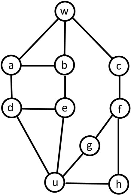
Figure 14. Initial graph

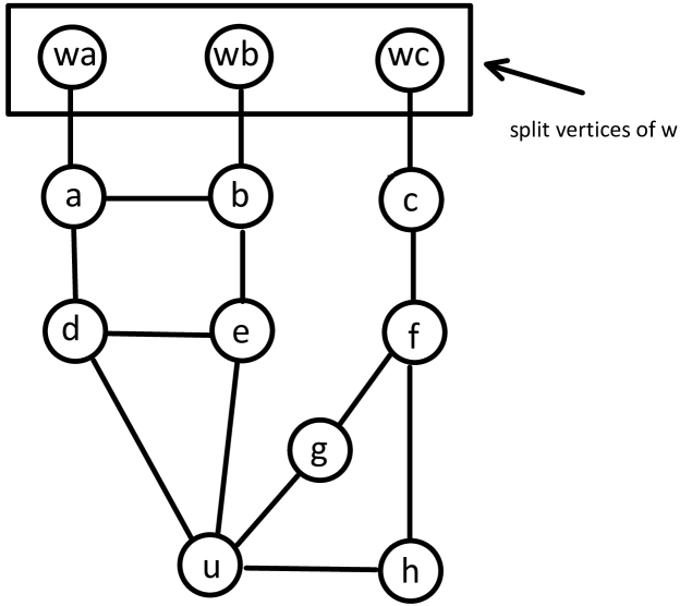
Figure 15. $w$-extension of $G$

11. Proof of Theorem 5.6

11.1. The Extended Influence Matrix

In this section, we introduce what we call the extended-influence matrix which we denote as ${\mathcal{H}}^{\Lambda,\tau}_{G}$. Similarly to the standard influence matrix ${{\mathcal{I}}}^{\Lambda,\tau}_{G}$, matrix ${\mathcal{H}}^{\Lambda,\tau}_{G}$ expresses influences between vertices however in a more refined, but also more involved setting.

We consider the graph $G=(V,E)$, a Gibbs distribution $\mu_{G}$ defined as in (2.1). Furthermore, we have $\Lambda\subset V$ and $\tau\in\{\pm\}^{\Lambda}$. Also, without loss of generality, assume that there is a total ordering of the vertices in graph $G$

In order to define the matrix ${\mathcal{H}}^{\Lambda,\tau}_{G}$, we need to introduce a few basic notions.

Graph extensions:

For a vertex $w\in V$, we let $G_{w}$ be the $w$-extension of $G$ which is the graph obtained by splitting $w$ into as many vertices as its degree. Specifically, we substitute vertex $w$ in $G$ with the split-vertices $ws$, one for each neighbour $s$ of $w$ in $G$. Furthermore, the split-vertex $ws$ is adjacent only to vertex $s$. For example, Fig. 15 shows graph $G_{w}$ which is the $w$-extension of graph $G$ in Fig. 15.

We let $S_{w}$ be the set of split-vertices of $G_{w}$, i.e., $S_{w}=\{ws\ |\ s\in N_{G}(w)\}$. Furthermore, let

$${\mathcal{S}}_{\Lambda} =\bigcup\nolimits_{w\in V\setminus\Lambda}S_{w}\enspace.$$ (11.1)

Note that for different $w,u\in V\setminus\Lambda$, the set $S_{w},S_{u}$ refer to different graphs.

Similarly to the above, for two vertices $u,w\in V\setminus\Lambda$ different from each other, we have the $\{u,w\}$-extension of graph $G$, denoted as $G_{u,w}$. For this graph we first obtain $G_{w}$ and then, we take the $u$-extension of $G_{w}$. Note that the order in which we take the extensions for $G_{w,u}$ does not really matter. Fig. 16 shows the $\{u,w\}$-extension of the graph from Fig. 15.

Also note that $\{u,w\}$-extension is well defined for any two vertices different from each other, e.g., we may have $u,w$ adjacent with each other, etc.

Extended Gibbs distribution:

For $G_{w}$ the $\{w\}$-extension of graph $G$, we introduce the notion of the extension for the Gibbs distribution $\mu^{\Lambda,\tau}_{G}$.

Specifically, for each $ws\in S_{w}$, we let the $ws$-extension of $\mu^{\Lambda,\tau}$ be the Gibbs distribution $\mu^{M,\sigma}_{G_{w}}$ on the graph $G_{w}$, with the same specifications as $\mu$, while for $(M,\sigma)$ we have the following:

$$M=(\Lambda\cup S_{w})\setminus\{ws\}\enspace,$$ (11.2)

that is, we obtain $M$ by taking the union of $\Lambda$ and all the split vertices of $w$ apart from $ws$. The configuration $\sigma\in\{\pm 1\}^{M}$ is such that for $v\in\Lambda\subseteq M$, we have $\sigma(v)=\tau(v)$, while for $wx\in S_{w}\setminus\{ws\}$ we have that

$$\sigma(wx) =\left\{\begin{array}[]{lcl}+1&&\textrm{if $w>x$}\enspace,\\ -1&&\textrm{if $w<x$}\enspace.\end{array}\right.$$ (11.5)

The comparison between $w,x$ is with respect to the total ordering of the vertices in $G$.

In the natural way we define the $\{ws,uz\}$-extension of $\mu^{\Lambda,\tau}_{G}$, when $w\neq u$. That is, suppose that $\mu^{M,\sigma}_{G_{w}}$ is the $ws$-extension of $\mu^{\Lambda,\tau}_{G}$. We take the $uz$-extension of $\mu^{M,\sigma}_{G_{w}}$ and obtain $\mu^{M^{\prime},\sigma^{\prime}}_{G_{w,u}}$. Then, $\mu^{M^{\prime},\sigma^{\prime}}_{G_{w,u}}$, is the $\{ws,uz\}$-extension of $\mu^{\Lambda,\tau}_{G}$.

Note that the $\{ws,uz\}$-extension of $\mu^{\Lambda,\tau}_{G}$ is a Gibbs distribution on $G_{u,w}$. Also, note that in the $\{ws,uz\}$-extension of $\mu^{\Lambda,\tau}_{G}$ apart from $ws$ and $uz$, all the spilt-vertices in $S_{w}$ and $S_{u}$ have a fixed configuration.

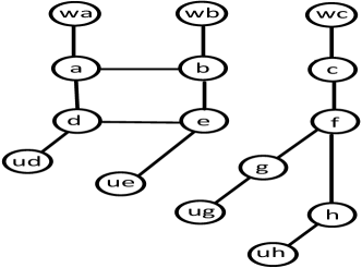
Figure 16. $\{u,w\}$-extension

The extended influence matrix

We now define the extended influence matrix ${\mathcal{H}}^{\Lambda,\tau}_{G}$. This is an ${\mathcal{S}}_{\Lambda}\times{\mathcal{S}}_{\Lambda}$ matrix with entries in the interval $[-1,1]$.

For $(ws,uz)\in{\mathcal{S}}_{\Lambda}\times{\mathcal{S}}_{\Lambda}$ such that $u\neq w$, while letting $\upnu(\cdot\ |\ (M,\sigma))$ be the $\{ws,uz\}$-extension of $\mu_{G}(\cdot\ |\ (\Lambda,\tau))$, we have that

$${\mathcal{H}}^{\Lambda,\tau}_{G}(ws,uz) =\upnu_{uz}(+1\ |\ (M,\sigma),(ws,+1))-\upnu_{uz}(-1\ |\ (M,\sigma),(ws,-1))\enspace.$$ (11.6)

That is, ${\mathcal{H}}^{\Lambda,\tau}_{G}(ws,uz)$ corresponds to the influence of the split-vertex $ws$ to the split-vertex $uz$ in $G_{w,u}$ under the Gibbs distribution $\upnu(\cdot\ |\ (M,\sigma))$. Hence, we have that

$${\mathcal{H}}^{\Lambda,\tau}_{G}(ws,uz) ={{\mathcal{I}}}^{M,\sigma}_{G_{w,u}}(ws,uz)\enspace,$$ (11.7)

where ${{\mathcal{I}}}^{M,\sigma}_{G_{w,u}}$ is specified with respect to $\upnu(\cdot\ |\ (M,\sigma))$. Furthermore, when $w=u$, we specify that ${\mathcal{H}}^{\Lambda,\tau}_{G}(ws,uz)=0$.

One major difference between ${\mathcal{H}}^{\Lambda,\tau}_{G}$ and the standard influence matrix ${{\mathcal{I}}}^{\Lambda,\tau}_{G}$ is that for different entries in the first matrix the underlying graph, or the conditioning might change.

Let be a $(V\setminus\Lambda)\times{\mathcal{S}}_{\Lambda}$, zero-one matrix such that for any $r\in V\setminus\Lambda$ and any $vx\in{\mathcal{S}}_{\Lambda}$ we have

$$\UpK(r,vx) =\mathds{1}\{r=v\}\enspace.$$ (11.8)

Similarly, let be a ${\mathcal{S}}_{\Lambda}\times(V\setminus\Lambda)$ zero-one matrix, such that for any $r\in V\setminus\Lambda$ and any $vx\in{\mathcal{S}}_{\Lambda}$ we have

$$\UpC(vx,r) =\mathds{1}\{v=r\}\enspace.$$ (11.9)

Remark 11.1.

We overload and to indicate both the matrices above and those in (9.6) and (9.5). This is because, up to a change of labelings, the corresponding matrices are identical.

Theorem 11.2.

Let ${\Delta}>1$, while let $\beta,\gamma,\lambda\in\mathbb{R}$ be such that $\gamma>0$, $0\leq\beta\leq\gamma$ and $\lambda>0$.

Let $G=(V,E)$ be of maximum degree ${\Delta}$. Consider $\mu_{G}$ the Gibbs distribution on $G$ specified by the parameters $(\beta,\gamma,\lambda)$, while assume that $(\beta,\gamma,\lambda)$ are such that $\mu_{G}$ is $b$-marginally bounded, for some $b>0$.

There exists an ${\mathcal{S}}_{\Lambda}\times{\mathcal{S}}_{\Lambda}$ matrix ${\mathcal{N}}$ such that for every $ws,uz\in{\mathcal{S}}_{\Lambda}$ we have $0\leq{\mathcal{N}}(ws,uz)\leq b^{-4}$, while for any $\Lambda\subset V$ and any $\tau\in\{\pm 1\}^{\Lambda}$ we have that

$${{\mathcal{I}}}^{\Lambda,\tau}_{G} =\UpI+\UpK\cdot\left({\mathcal{H}}^{\Lambda,\tau}_{G}\circ{\mathcal{N}}\right)\cdot\UpC\enspace,$$

where ${\mathcal{H}}^{\Lambda,\tau}_{G}\circ{\mathcal{N}}$ is the Hadamard product of the two matrices.

The proof of Theorem 11.2 appears in Section 12.

In what follows, for the graph $G_{w}$, i.e., the $\{w\}$-extension of $G$, and for $ws\in S_{w}$, we let $T_{{\rm SAW}}(G_{w},ws)$ be the tree of self-avoiding walks that starts from the split-vertex $ws$.

Theorem 11.3.

Let ${\Delta}>1$, $s\geq 1$, allowing $s=\infty$, let $\delta,c\in\mathbb{R}_{>0}$. Also, let $\beta,\gamma,\lambda\in\mathbb{R}$ be such that $\gamma>0$, $0\leq\beta\leq\gamma$ and $\lambda>0$. Consider the graph $G=(V,E)$ of maximum degree ${\Delta}$, while let $\mu$ the Gibbs distribution on $G$ specified by the parameters $(\beta,\gamma,\lambda)$.

Suppose that there is a $(s,\delta,c)$-potential function ${\Psi}$ with respect to $(\beta,\gamma,\lambda)$. Then, for any $\Lambda\subset V$, for any $\tau\in\{\pm 1\}^{\Lambda}$, for any diagonal, non-negative, non-singular ${\mathcal{S}}_{\Lambda}\times{\mathcal{S}}_{\Lambda}$ matrix we have that

$$\left|\left|{}^{-1}\cdot{\mathcal{H}}^{\Lambda,\tau}_{G}\cdot\UpD\right|\right|_{\infty} \leq\max_{wx\in{\mathcal{S}}_{\Lambda}}\left\{\frac{c}{\UpD(wx,wx)}\left(\UpD(xw,xw)+\sum\nolimits_{\ell\geq 2}\left(\sum\nolimits_{uz\in{\mathcal{S}}_{\Lambda}}{\tt A}(uz,\ell)\cdot\delta^{\ell-1}\cdot{}^{s}(uz,uz)\right)^{1/s}\right)\right\}\enspace,$$

where ${\tt A}(uz,\ell)$ is the set of copies of split-vertex $uz$ in ${T_{\rm SAW}}(G_{w},wx)$.

The proof of Theorem 11.3 appears in Section 13.

11.2. Proof of Theorem 5.6

Using Theorem 11.2 and working as in Theorem 8.1, we get the following: for any diagonal, non-negative, non-singular ${\mathcal{S}}_{\Lambda}\times{\mathcal{S}}_{\Lambda}$ matrix we have that

$$\left|\left|{{\mathcal{I}}}^{\Lambda,\tau}_{G}\right|\right|_{2} \leq 1+{\Delta}\cdot\textstyle\max\left\{\left|\left|{}^{-1}\cdot\left({\mathcal{H}}^{\Lambda,\tau}_{G}\circ{\mathcal{N}}\right)\cdot\UpD\right|\right|_{\infty},\ \left|\left|{}^{-1}\cdot\bar{{\mathcal{H}}}^{\Lambda,\tau}_{G}\circ\bar{{\mathcal{N}}}\cdot\UpD\right|\right|_{\infty}\right\}\enspace.$$

Furthermore, since for every $ws,uz\in{\mathcal{S}}_{\Lambda}$ we have $0\leq{\mathcal{N}}(ws,uz)\leq b^{-4}$ we get that

$$\left|\left|{{\mathcal{I}}}^{\Lambda,\tau}_{G}\right|\right|_{2} \leq 1+b^{-4}\cdot{\Delta}\cdot\textstyle\max\left\{\left|\left|{}^{-1}\cdot\ {\mathcal{H}}^{\Lambda,\tau}_{G}\cdot\UpD\right|\right|_{\infty},\ \left|\left|{}^{-1}\cdot\bar{{\mathcal{H}}}^{\Lambda,\tau}_{G}\cdot\UpD\right|\right|_{\infty}\right\}\enspace.$$ (11.10)

Claim 11.4.

We have that

$$\textstyle\left|\left|{}^{-1}\cdot\bar{{\mathcal{H}}}^{\Lambda,\tau}_{G}\cdot\UpD\right|\right|_{\infty} \leq b^{-2}\cdot\left|\left|{}^{-1}\cdot{\mathcal{H}}^{\Lambda,\tau}_{G}\cdot\UpD\right|\right|_{\infty}.$$ (11.11)

Proof.

We show that for any $ws,uz\in{\mathcal{S}}_{\Lambda}$ we have that

$${\mathcal{H}}^{\Lambda,\tau}_{G}(ws,uz)\leq b^{-2}\cdot{\mathcal{H}}^{\Lambda,\tau}_{G}(uz,ws)\enspace.$$ (11.12)

Then, it is a matter of elementary derivations to show that indeed (11.11) is true. For the case where $w=u$, both matrix entries in (11.12) are zero, hence the inequality is trivially true.

We now focus on the case where $w\neq u$. Then, as already noticed in (11.7) we have that

$${\mathcal{H}}^{\Lambda,\tau}_{G}(ws,uz) ={{\mathcal{I}}}^{M,\sigma}_{G_{w,u}}(ws,uz), {\mathcal{H}}^{\Lambda,\tau}_{G}(uz,ws) ={{\mathcal{I}}}^{M,\sigma}_{G_{w,u}}(uz,ws)\enspace.$$ (11.13)

Both entries ${{\mathcal{I}}}^{M,\sigma}_{G_{w,u}}(ws,uz)$ and ${{\mathcal{I}}}^{M,\sigma}_{G_{w,u}}(uz,ws)$ are with respect to the measure $\upnu^{M,\sigma}$ which is the $\{ws,uz\}$-extension of $\mu^{\Lambda,\tau}_{G}$. Recall that $\upnu^{M,\sigma}$ is a Gibbs distribution on $G_{w,u}$, where $(M,\sigma)$ is obtained from $(\Lambda,\tau)$.

Then, from Claim 4.1 we have that

$${{\mathcal{I}}}^{M,\sigma}_{G_{w,u}}(ws,uz) =\frac{\upnu^{M,\sigma}_{uz}(1)\cdot\upnu^{M,\sigma}_{uz}(-1)}{\upnu^{M,\sigma}_{ws}(1)\cdot\upnu^{M,\sigma}_{ws}(-1)}\cdot{{\mathcal{I}}}^{M,\sigma}_{G_{w,u}}(uz,ws)\enspace.$$ (11.14)

Combining (11.14) and (11.13) we get that

$${\mathcal{H}}^{\Lambda,\tau}_{G}(ws,uz) =\frac{\upnu^{M,\sigma}_{uz}(1)\cdot\upnu^{M,\sigma}_{uz}(-1)}{\upnu^{M,\sigma}_{ws}(1)\cdot\upnu^{M,\sigma}_{ws}(-1)}\cdot{\mathcal{H}}^{\Lambda,\tau}_{G}(uz,ws)\enspace.$$ (11.15)

Then, (11.12) follows noting that $\max_{ws,uz}\left\{\frac{\upnu^{M,\sigma}_{uz}(1)\cdot\upnu^{M,\sigma}_{uz}(-1)}{\upnu^{M,\sigma}_{ws}(1)\cdot\upnu^{M,\sigma}_{ws}(-1)}\right\}\leq b^{-2}$. The bound follows by noting that, since $\mu^{\Lambda,\tau}_{G}$ is assumed to be $b$-marginally bounded, we have that $\upnu^{M,\sigma}$ is $b$-marginally bounded, too.

All the above conclude the proof of Claim 11.4. ∎

Plugging the bound from Claim 11.4 into (11.10) we get that

$$\left|\left|{{\mathcal{I}}}^{\Lambda,\tau}_{G}\right|\right|_{2} \leq 1+b^{-6}\cdot{\Delta}\cdot\textstyle\left|\left|{}^{-1}\cdot\ {\mathcal{H}}^{\Lambda,\tau}_{G}\cdot\UpD\right|\right|_{\infty}\enspace.$$ (11.16)

Let ${\upkappa}_{1}$ be the eigenvector that corresponds to the maximum eigenvalue of _G. Recall that ${\upkappa}_{1}$ is indexed by $M$, the set of oriented edges of $G$. Note that since we have assumed that _G is irreducible, for any $xv\in M$ we have that

$${\upkappa}_{1}(xv)>0\enspace.$$ (11.17)

Let $\Upphi$ be the ${\mathcal{S}}_{\Lambda}\times{\mathcal{S}}_{\Lambda}$ diagonal matrix such that for any $xv\in{\mathcal{S}}_{\Lambda}$ we have that

$$\Upphi(xv,xv) ={\upkappa}_{1}(vx)\enspace,$$ (11.18)

note that the argument $vx$ refers to the oriented edge from $v$ to $x$. One needs to be cautious about the direction of the edge in the component of ${\upkappa}_{1}$ for the diagonal entries of $\Upphi$.

We further note that, due to (11.17), the diagonal entries of $\Upphi$ are all positive, hence the matrix is non-singular. Setting $\UpD=\Upphi$ in (11.16) we get that

$$\left|\left|{{\mathcal{I}}}^{\Lambda,\tau}_{G}\right|\right|_{2} \leq 1+b^{-6}\cdot{\Delta}\cdot\textstyle\left|\left|\Upphi^{-1}\cdot{\mathcal{H}}^{\Lambda,\tau}_{G}\cdot\Upphi\right|\right|_{\infty}\enspace.$$ (11.19)

Then, using Theorem 11.3 and working as in the proof of Theorem 5.5 we get that

$$\left|\left|\Upphi^{-1}\cdot{\mathcal{H}}^{\Lambda,\tau}_{G}\cdot\Upphi\right|\right|_{\infty} \leq c\cdot(1-(1-\varepsilon)^{1/s})^{-1}\cdot\max_{wx\in{\mathcal{S}}_{\Lambda}}\left\{{\textstyle\left(\frac{{\upkappa}_{1}(wx)}{{\upkappa}_{1}(xw)}\right)^{1/s}}\right\}$$

$$\leq\frac{\zeta}{\uptheta}\cdot{\hat{c}}\cdot(1-(1-\varepsilon)^{1/s})^{-1}\enspace.$$

The last inequality follows since we have assumed that ${}_{G}\in{\mathbb{H}}_{n,{\hat{c}}}$ while $c=\zeta/\uptheta$. Then, we have that

$$\left|\left|{{\mathcal{I}}}^{\Lambda,\tau}_{G}\right|\right|_{2} \leq 1+b^{-6}\cdot\zeta\cdot{\hat{c}}\cdot(1-(1-\varepsilon)^{1/s})^{-1}\cdot{\Delta}/\uptheta\enspace.$$

The above conclude the proof of Theorem 5.6. $\Box$

12. Proof of Theorem 11.2

Let ${\mathcal{F}}^{\Lambda,\tau}_{G}$ be the ${\mathcal{S}}_{\Lambda}\times(V\setminus\Lambda)$ matrix such that the entry ${\mathcal{F}}^{\Lambda,\tau}_{G}(sw,v)$ is as follows: letting $\upzeta(\cdot\ |\ (N,\xi))$ be the $ws$-extension of $\mu^{\Lambda,\tau}_{G}$, for $w\neq v$ we have

$${\mathcal{F}}^{\Lambda,\tau}_{G}(ws,v) =\upzeta_{v}(+1\ |\ (N,\xi),\ (ws,+1))-\upzeta_{v}(+1\ |\ (N,\xi),(ws,-1))\enspace,$$ (12.1)

If $w=v$, then ${\mathcal{F}}^{\Lambda,\tau}_{G}(ws,v)=0$.

Lemma 12.1.

We have that ${{\mathcal{I}}}^{\Lambda,\tau}_{G}=\UpI+\UpK\cdot{\mathcal{F}}^{\Lambda,\tau}_{G}.$

Lemma 12.2.

We have that ${\mathcal{F}}^{\Lambda,\tau}_{G}=\left({\mathcal{H}}^{\Lambda,\tau}_{G}\circ{\mathcal{N}}\right)\cdot\UpC$.

Theorem 11.2 follows as a corollary from Lemmas 12.1 and 12.2. $\Box$

12.1. Proof of Lemma 12.1

Firstly, note that both ${{\mathcal{I}}}^{\Lambda,\tau}_{G}$ and $\UpI+\UpK\cdot{\mathcal{F}}^{\Lambda,\tau}_{G}$ are $(V\setminus\Lambda)\times(V\setminus\Lambda)$ matrices.

For brevity we use ${\mathcal{F}}$ and ${{\mathcal{I}}}$ to denote ${\mathcal{F}}^{\Lambda,\tau}_{G}$ and ${{\mathcal{I}}}^{\Lambda,\tau}_{G}$, respectively. From the definition of the matrices ${\mathcal{F}},\UpK$ it is a simple calculation to show that

$$\left(\UpK\cdot{\mathcal{F}}\right)(v,v) =0 v\in V\setminus\Lambda\enspace.$$

The above implies that both ${{\mathcal{I}}}$ and $\UpI+\UpK\cdot{\mathcal{F}}$ have ones at their diagonal. We focus on the off-diagonal diagonal elements. It suffices to show that for any $u,w\in V\setminus\Lambda$, different from each other, we have that

$${{\mathcal{I}}}(w,u) =\sum\nolimits_{ws\in S_{w}}{\mathcal{F}}(ws,v)\enspace,$$ (12.2)

where recall that $S_{w}$ is the set of split-vertices in $G_{w}$.

Let $T=T_{{\rm SAW}}(G,w)$ be the tree of self-avoiding walks in $G$ that starts from $w$. Also, let $\{\upbeta(e)\}$ be the collection of weights over the edges of $T$ we obtain as described in (6.3). From Proposition 6.1 we have that

$${{\mathcal{I}}}(w,u) =\sum\nolimits_{P\in{\mathcal{M}}}\prod\nolimits_{e\in P}\upbeta(e)\enspace,$$ (12.3)

where ${\mathcal{M}}$ consists of all paths from the root of ${T_{\rm SAW}}(w)$ to the set of copies of $u$ in $T$.

Consider now $G_{w}$ the $w$-extension of $G$. Then, for $ws\in S_{w}$ let $\upzeta(\cdot\ |\ (N,\xi))$ be the $w$-extension of $\mu^{\Lambda,\tau}_{G}$. Since $\upzeta(\cdot\ |\ (N,\xi))$ is a Gibbs distribution on $G_{w}$, we apply the construction we describe in Section 6. Specifically, let $T_{s}=T_{{\rm SAW}}(ws)$ be the tree of self-avoiding walks in $G_{w}$ that starts from $ws$. We, also, let $\{\upbeta_{s}(e)\}$ be the collection of weights over the edges of $T_{s}$ we obtain as described in (6.3).

Clearly, Proposition 6.1 implies that

$${\mathcal{F}}(ws,u) =\sum\nolimits_{P\in{\mathcal{M}}_{s}}\prod\nolimits_{e\in P}\upbeta_{s}(e)\enspace,$$ (12.4)

where ${\mathcal{M}}_{s}$ consists of all paths from the root of ${T_{\rm SAW}}(ws)$ to the set of copies of $u$ in $T_{s}$.

The above constructions have some properties that need highlighting: Firstly, note that $T_{s}$ is identical to the subtree of $T$ which is induced by the root of $T$, the child of the root which is a copy of $s$, as well as the descendent of this vertex. Hence, we rearrange the sum in (12.3) and get that

$${{\mathcal{I}}}(w,u) =\sum\nolimits_{s}\sum\nolimits_{P\in{\mathcal{M}}_{s}}\prod\nolimits_{e\in P}\upbeta(e)\enspace.$$ (12.5)

Secondly, if we identify $T_{s}$ as a subtree of $T$, then for all $e\in T_{s}$ we have that

$$\upbeta_{s}(e) =\upbeta(e)\enspace.$$ (12.6)

To see the above, note that the weights $\upbeta(e)$ and $\upbeta_{s}(e)$ do not depend on the marginal distribution at the root of the corresponding tree. Furthermore, the copy of vertex $s$ that is a child of the root in $T$ has the same marginal distribution as the corresponding copy of $s$ in the tree $T_{s}$. Hence, it is straightforward that the rest of the construction gives the same weights for the two trees.

Combining (12.5) and (12.6), we get that

$${{\mathcal{I}}}(w,u) =\sum\nolimits_{s}\sum\nolimits_{P\in{\mathcal{M}}_{s}}\prod\nolimits_{e\in P}\upbeta_{s}(e)=\sum\nolimits_{s}{\mathcal{F}}(ws,u)\enspace.$$ (12.7)

For the last equality we use (12.4).

Lemma 12.1 follows by noting that (12.7) implies (12.2). $\Box$

12.2. Proof of Lemma 12.2

Before we start our proof, it is useful to notice that Lemma 12.1 implies that the influence matrix ${{\mathcal{I}}}^{\Lambda,\tau}_{G}$ satisfies the following relation: for any $w,u\in V\setminus\Lambda$ we have that

$${{\mathcal{I}}}^{\Lambda,\tau}_{G}(w,u) =\sum\nolimits_{ws\in S_{w}}{{\mathcal{I}}}^{M_{s},\sigma_{s}}_{G_{w}}(ws,u)\enspace,$$ (12.8)

where note that on the r.h.s. the influence matrix is with respect to $G_{w}$ and $\upzeta(\cdot\ |\ M_{s},\sigma_{s})$, i.e., the $ws$-extension of $G$ and the Gibbs distribution $\mu^{\Lambda,\tau}_{G}$. The boundary condition $(M_{s},\sigma_{s})$ is obtained as we describe in (11.2) and (11.5). We use the subscripts to indicate the dependence of the condition on $ws$. We use this observation later in the proof.

The lemma follows by showing that for any $w,u\in V\setminus\Lambda$ and any split-vertex $ws\in S_{w}$, we have that

$${\mathcal{F}}^{\Lambda,\tau}_{G}(ws,u) =\sum\nolimits_{uz\in S_{u}}{\mathcal{N}}(ws,uz)\cdot{\mathcal{H}}^{\Lambda,\tau}_{G}(ws,uz)\enspace.$$ (12.9)

where ${\mathcal{N}}$ is the same matrix as that in the statement of Theorem 11.2 and is specified later.

From the definition of ${\mathcal{F}}^{\Lambda,\tau}_{G}$, we have that ${\mathcal{F}}^{\Lambda,\tau}_{G}(ws,u)$ is the influence of $ws$ to $u$ under the measure $\upzeta^{M_{s},\sigma_{s}}$, which is the $ws$-extension of $\mu^{\Lambda,\tau}_{G}$. That is,

$${\mathcal{F}}^{\Lambda,\tau}_{G}(ws,u) ={{\mathcal{I}}}^{M_{s},\sigma_{s}}_{G_{w}}(ws,u)=\frac{\upzeta^{M_{s},\sigma_{s}}_{u}(1)\cdot\upzeta^{M_{s},\sigma_{s}}_{u}(-1)}{\upzeta^{M_{s},\sigma_{s}}_{ws}(1)\cdot\upzeta^{M_{s},\sigma_{s}}_{ws}(-1)}\cdot{{\mathcal{I}}}^{M_{s},\sigma_{s}}_{G_{w}}(u,ws)\enspace.$$ (12.10)

The second equality follows from Claim 4.1.

Furthermore, applying (12.8) to the entry ${{\mathcal{I}}}^{M_{s},\sigma_{s}}_{G_{w}}(u,ws)$ we get that

$${{\mathcal{I}}}^{M_{s},\sigma_{s}}_{G_{w}}(u,ws) =\sum\nolimits_{uz\in S_{u}}{{\mathcal{I}}}^{M_{s,z},\sigma_{s,z}}_{G_{w,u}}(uz,ws)=\sum\nolimits_{uz\in S_{u}}{\mathcal{H}}^{\Lambda,\tau}_{G}(uz,ws)\enspace.$$ (12.11)

For the influence matrices in the sum in the middle part, note that each one of them is with respect to the $\{uz\}$-extension of $\upzeta^{M_{s},\sigma_{s}}$. Let us call this measure $\upnu^{M_{s,z},\sigma_{s,z}}$, while note that this is the $\{ws,uz\}$-extension of $\mu^{\Lambda,\tau}_{G}$. The second equality follows from the definition of ${\mathcal{H}}^{\Lambda,\tau}_{G}$, i.e., we have that

$${{\mathcal{I}}}^{M_{s,z},\sigma_{s,z}}_{G_{w,u}}(uz,ws) ={\mathcal{H}}^{\Lambda,\tau}_{G}(uz,ws) \forall uz\in S_{u}\enspace.$$

With the above equality in mind, we apply Claim 4.1 once more and get that

$${\mathcal{H}}^{\Lambda,\tau}_{G}(uz,ws) =\frac{\upnu^{M_{s,z},\sigma_{s,z}}_{ws}(1)\cdot\upnu^{M_{s,z},\sigma_{s,z}}_{ws}(-1)}{\upnu^{M_{s,z},\sigma_{s,z}}_{uz}(1)\cdot\upnu^{M_{s,z},\sigma_{s,z}}_{uz}(-1)}\cdot{\mathcal{H}}^{\Lambda,\tau}_{G}(ws,uz)\enspace.$$ (12.12)

Plugging (12.11) and (12.12) into (12.10) we get that

$${\mathcal{F}}^{\Lambda,\tau}_{G}(ws,u) =\sum_{uz\in S_{u}}\frac{\upzeta^{M_{s},\sigma_{s}}_{u}(1)\cdot\upzeta^{M_{s},\sigma_{s}}_{u}(-1)}{\upzeta^{M_{s},\sigma_{s}}_{ws}(1)\cdot\upzeta^{M_{s},\sigma_{s}}_{ws}(-1)}\cdot\frac{\upnu^{M_{s,z},\sigma_{s,z}}_{ws}(1)\cdot\upnu^{M_{s,z},\sigma_{s,z}}_{ws}(-1)}{\upnu^{M_{s,z},\sigma_{s,z}}_{uz}(1)\cdot\upnu^{M_{s,z},\sigma_{s,z}}_{uz}(-1)}\cdot{\mathcal{H}}^{\Lambda,\tau}_{G}(ws,uz)\enspace.$$ (12.13)

We set ${\mathcal{N}}(ws,uz)$ equal to the coefficient of ${\mathcal{H}}^{\Lambda,\tau}_{G}(ws,uz)$ in the above sum.

It remains to prove that for every $ws,uz\in{\mathcal{S}}_{\Lambda}$ we have $0\leq{\mathcal{N}}(ws,uz)\leq b^{-4}$. Since $\mu^{\Lambda,\tau}_{G}$ is assumed to be $b$-marginally bounded, it is straightforward that $\upzeta^{M_{s},\sigma_{s}}$ and $\upnu^{M_{s,z},\sigma_{s,z}}$ are $b$-marginally bounded, too. Recall that both have the same specifications as $\mu^{\Lambda,\tau}_{G}$. This implies that indeed $0\leq{\mathcal{N}}(ws,uz)\leq b^{-4}$.

Lemma 12.2 follows. $\Box$

13. Proof of Theorem 11.3

In what follows, for the diagonal matrix , we abbreviate $\UpD(wx,wx)$ to $\UpD(wx)$.

For $wx,uz\in{\mathcal{S}}_{\Lambda}$ such that $w\neq u$, the entry ${\mathcal{H}}^{\Lambda,\tau}_{G}(wx,uz)$ corresponds to the influence of $wx$ to $uz$ in the graph $G_{w,u}$ under the $\{wx,uz\}$-extension of $\mu^{\Lambda,\tau}_{G}$. Let the Gibbs distribution on $\upnu^{M,\sigma}_{G_{u,w}}$ be the $\{wx,uz\}$-extension of $\mu^{\Lambda,\tau}_{G}(\cdot)$.

Since ${\mathcal{H}}^{\Lambda,\tau}_{G}(wx,uz)$ is an influence, we consider the construction Section 6. Specifically, let $T=T_{{\rm SAW}}(G_{u,w},wx)$, while let the weights $\{\upbeta_{{uz}}(e_{i})\}$ be obtained as we describe in (6.3) with respect to $\upnu^{M,\sigma}_{G_{u,w}}$. Note that $(M,\sigma)$ and hence $\{\upbeta_{{uz}}(e_{i})\}$ depend on the $wx,uz$.

For every path $P=e_{1},e_{2},\ldots,e_{\ell}$, that starts from the root of the tree $T$, let

$${\tt weight}_{uz}(P)=\prod\nolimits_{i\in[\ell]}\upbeta_{uz}(e_{i})\enspace.$$

Let ${\mathcal{Q}}^{(\ell,uz)}_{\rm root}$ be defined by

$${\mathcal{Q}}^{(\ell,uz)}_{\rm root} =\frac{\UpD(uz)}{\UpD(wx)}\cdot\sum\nolimits_{P\in{\mathcal{P}}_{uz}}\left|{\tt weight}_{uz}(P)\right|\enspace,$$ (13.1)

where ${\mathcal{P}}_{uz}$ is the set of all paths from the root of $T$ to the vertices in ${\tt A}(uz,\ell)$, i.e., the set of vertices at level $\ell$ of the tree $T$ which are copies of the split-vertex $uz$. Also, let

$${\mathcal{Q}}^{(\ell)}_{\rm root} =\sum\nolimits_{uz\in{\mathcal{S}}_{\Lambda}}{\mathcal{Q}}^{(\ell,uz)}_{\rm root}\enspace.$$

It is clear that

$$\sum\nolimits_{uz\in S_{u}}\left|\left({}^{-1}\cdot{\mathcal{H}}^{\Lambda,\tau}_{G}\cdot\UpD\right)(wx,vz)\right| \leq\sum\nolimits_{\ell\geq 1}{\mathcal{Q}}^{(\ell)}_{\rm root}\enspace.$$ (13.2)

The theorem follows by showing for any $wx\in{\mathcal{S}}_{\Lambda}$ and any $\ell>1$, we have that

$${\mathcal{Q}}^{(\ell)}_{\rm root} \leq\frac{c}{\UpD(wx)}\cdot\left(\sum\nolimits_{uz\in{\mathcal{S}}_{\Lambda}}|{\tt A}(uz,\ell)|\cdot\delta^{\ell-1}\cdot{}^{s}(uz)\right)^{1/s}\enspace,$$ (13.3)

while for $\ell=1$, we have that

$${\mathcal{Q}}^{(\ell)}_{\rm root}\leq c\cdot\frac{\UpD(xw)}{\UpD(wx)}\enspace.$$ (13.4)

In order to prove (13.3) we use the following result, which is useful to involve the potential function ${\Psi}$ in our derivations.

Claim 13.1.

For any $uz\in S_{u}$, for any path $P=e_{1},\ldots,e_{\ell}$ of length $\ell>1$, that starts from the root of the tree $T_{{\rm SAW}}(G_{u,w},wx)$, we have that

$${\tt weight}_{uz}(P) =\upgamma_{uz}(e_{\ell})\cdot\frac{\upbeta_{uz}(e_{1})}{\upgamma_{uz}(e_{1})}\cdot\prod^{\ell}_{i=2}\frac{\upgamma_{uz}(e_{i-1})}{\upgamma_{uz}(e_{i})}\cdot\upbeta_{uz}(e_{i})\enspace,$$

where $\upgamma_{uz}(e)=\chi(\upbeta_{uz}(e))$ and $\chi={\Psi}^{\prime}$.

The proof of Claim 13.1 is identical to that of Claim 10.2, i.e., we use the same telescopic trick. For this reason, we omit it.

Consider the vertex $v$ in the tree $T$, at level $0\leq h<\ell$. As before, let $T_{v}$ be the subtree that contains $v$ and all its descendants. Let the quantity ${\mathcal{R}}^{uz}_{v}$ be defined by

$${\mathcal{R}}^{uz}_{v}=\frac{\UpD(uz)}{\UpD(wx)}\cdot\sum_{P\in{\mathcal{P}}^{uz}_{u}}\prod^{\ell-h}_{i=1}\frac{\upgamma_{uz}(e_{i-1})}{\upgamma_{uz}(e_{i})}\cdot\left|\upbeta_{uz}(e_{i})\right|\enspace,$$

where ${\mathcal{P}}^{vz}_{u}$ is the set of paths from the root of $T_{v}$ to the vertices in $T_{v}\cap{\tt A}(uz,\ell)$, while we take $P$ such that $P=e_{1},\ldots,e_{\ell-h}$ and $e_{0}$ is the edge that connects $v$ with its parent.

For a vertex $v\in T$ at level $h=\ell$ we set

$${\mathcal{R}}^{uz}_{v}=\sum\nolimits_{uz\in{\mathcal{S}}_{\Lambda}}\frac{\UpD(uz)}{\UpD(wx)}\cdot\mathds{1}\{v\in{\tt A}(uz,\ell)\}\enspace.$$ (13.5)

For $h=0$, i.e., having vertex $v$ to be the roof of $T$, we have ${\mathcal{R}}^{uz}_{v}={\mathcal{Q}}^{(\ell,uz)}_{wx}$. This follows from (13.1).

A simple induction implies that $R^{uz}_{v}$, for vertex $v$ being at level $0<h<\ell$ of the tree $T$, satisfied the following recursive relation: let $v_{1},\ldots,v_{d}$ be the children of $v$ in $T_{v}$, while let $a_{1},\ldots,a_{d}$ be the edges that connect $v$ with its children, i.e., the edge $a_{j}$ connects $v$ to $v_{j}$, etc. Then, we have that

$${\mathcal{R}}^{uz}_{v} =\upgamma_{uz}(a_{0})\cdot\sum\nolimits_{i\in[d]}\frac{\left|\upbeta_{uz}(a_{i})\right|}{\upgamma_{uz}(a_{0})}\cdot{\mathcal{R}}^{uz}_{v_{i}}\enspace,$$ (13.6)

where $a_{0}$ is the edge that connects $v$ to its parent in the tree $T$.

We further consider the quantity ${\mathcal{R}}_{v}$ defined by

$${\mathcal{R}}_{v} =\sum\nolimits_{uz\in{\mathcal{S}}_{\Lambda}}{\mathcal{R}}^{uz}_{v}\enspace.$$

Then, (13.6) implies that for a vertex $v$ at level $0<h<\ell$, we have that

$${\mathcal{R}}_{v} =\sum\nolimits_{uz\in{\mathcal{S}}_{\Lambda}}{\mathcal{R}}^{uz}_{v}\ =\ \sum\nolimits_{uz\in{\mathcal{S}}_{\Lambda}}\upgamma_{uz}(a_{0})\cdot\sum\nolimits_{i}\frac{\left|\upbeta_{uz}(a_{i})\right|}{\upgamma_{uz}(a_{0})}\cdot{\mathcal{R}}^{uz}_{v_{i}}$$

$$=\sum\nolimits_{i}\sum\nolimits_{uz\in{\mathcal{S}}_{\Lambda}}\upgamma_{uz}(a_{0})\cdot\frac{\left|\upbeta_{uz}(a_{i})\right|)}{\upgamma_{uz}(a_{0})}\cdot{\mathcal{R}}^{uz}_{v_{i}}$$

$$\leq\sum\nolimits_{i}\max\nolimits_{uz\in{\mathcal{S}}_{\Lambda}}\left\{\upgamma_{uz}(a_{0})\cdot\frac{\left|\upbeta_{uz}(a_{i})\right|}{\upgamma_{uz}(a_{0})}\right\}\sum\nolimits_{uz\in{\mathcal{S}}_{\Lambda}}{\mathcal{R}}^{uz}_{v_{i}}$$

$$\leq\sum\nolimits_{i}\max_{uz\in{\mathcal{S}}_{\Lambda}}\left\{\upgamma_{uz}(a_{0})\cdot\frac{\left|\upbeta_{uz}(a_{i})\right|}{\upgamma_{uz}(a_{0})}\right\}{\mathcal{R}}_{v_{i}}\enspace.$$

Combining the above inequality with our assumption about the $(s,\delta,c)$-potential, i.e., the contraction property, we get that

$$\left({{\mathcal{R}}}_{v}\right)^{s}\leq\delta\cdot\sum\nolimits_{v_{i}}\left({\mathcal{R}}_{v_{i}}\right)^{s}\enspace.$$

Then, a simple induction proves that

$$\left({{\mathcal{R}}}_{v}\right)^{s} \leq\sum\nolimits_{uz\in{\mathcal{S}}_{\Lambda}}\left(\frac{\UpD(uz)}{\UpD(wx)}\right)^{s}\cdot\delta^{\ell-h}\cdot|{\tt A}(uz,\ell)\cap T_{v}|\enspace,$$

where recall that $0<h<\ell$ is the level of vertex $v$ in the tree $T$.

Focusing on vertex $\pi$ the single child of the root of $T$, the above implies that

$$\left({{\mathcal{R}}}_{\pi}\right)^{s} \leq\sum\nolimits_{uz\in{\mathcal{S}}_{\Lambda}}\left(\frac{\UpD(uz)}{\UpD(wx)}\right)^{s}\cdot\delta^{\ell-1}\cdot|{\tt A}(uz,\ell)|\enspace.$$ (13.7)

For the above inequality, we observe that, since the root of $T$ has only vertex $\pi$ as a child and $\ell>1$, then we have that ${\tt A}(uz,\ell)\cap T_{c}={\tt A}(uz,\ell)$. Furthermore, it is not hard to see that

$${{\mathcal{Q}}}^{(\ell)}_{\rm root} \leq\max_{uz}\max_{e_{a},e_{b}\in T}\left\{\upgamma_{uz}(e_{a})\cdot\frac{|\upbeta_{uz}(e_{b})|}{\upgamma_{uz}(e_{b})}\right\}\cdot{{\mathcal{R}}}_{\pi}\enspace.$$

Our assumption about the $(s,\delta,c)$-potential, i.e., the boundedness property, implies that

$${{\mathcal{Q}}}^{(\ell)}_{\rm root} \leq c\cdot{{\mathcal{R}}}_{\pi}\enspace.$$ (13.8)

Then (13.3) follows by plugging (13.7) into (13.8).

As far as ${{\mathcal{Q}}}^{(1)}_{\rm root}$ is concerned, note the following: for any $e\in T$ and any $uz\in{\mathcal{S}}_{\Lambda}$ we have that

$$|\upbeta_{uz}(e)|=\frac{\upgamma_{uz}(e)}{\upgamma_{uz}(e)}\cdot|\upbeta_{uz}(e)|\leq\max_{\bar{e},\hat{e}\in T}\left\{\upgamma_{uz}(\bar{e})\cdot\frac{|\upbeta_{uz}(\hat{e})|}{\upgamma_{uz}(\hat{e})}\right\}\leq c\enspace,$$ (13.9)

where the last inequality follows from our assumption about $(s,\delta,c)$-potential, i.e., “Boundedness”. From the definition of ${{\mathcal{Q}}}^{(1)}_{\rm root}$, we have that

$${{\mathcal{Q}}}^{(1)}_{\rm root} =\frac{1}{\UpD(wx)}\UpD(xw)\cdot\left|\upbeta_{xw}(e)\right|\leq c\cdot\frac{\UpD(xw)}{\UpD(wx)}\enspace.$$ (13.10)

In the last inequality we use (13.9). The above proves (13.4).

Having proved that both (13.3) and (13.4) are true, concludes the proof of Theorem 11.3. $\Box$

14. Proof of results in Section 2 - Ising Model

For $d>0$, consider the functions $H_{d}$ and $h(\cdot)$ defined in (5.3) and (5.4), respectively. Recall that the zero external field Ising model $\mu$ corresponds to setting the parameters $\beta,\gamma$ and $\lambda$ such that $\beta=\gamma$ and $\lambda=1$. We have that

$$H_{d}:[-\infty,+\infty]^{d}\to[-\infty,+\infty] (x_{1},\ldots,x_{d})\mapsto\sum\nolimits_{i\in[d]}\log\left(\frac{\beta\exp(x_{i})+1}{\exp(x_{i})+\beta}\right)\enspace.$$ s.t. (14.1)

Since $\frac{\partial}{\partial x_{i}}H_{d}(x_{1},\ldots,x_{d})=h(x_{i})$, we have that

$$h(x) =-\frac{(1-\beta^{2})\exp(x)}{(\beta\exp(x)+1)(\exp(x)+\beta)}\enspace.$$ (14.2)

The following is a folklore result.

Lemma 14.1.

For any $d>0$, $\zeta\in(0,1)$, $R>1$ and $\beta\in{\mathbb{U}_{\rm Ising}}(R,\zeta)$ we have the following: the functions $H_{d}$ specified in (14.1) satisfies that

$$||\nabla H_{d}({y}_{1},{y}_{2},\ldots,{y}_{d})||_{\infty} \leq{(1-\zeta)}/{R}\enspace.$$ (14.3)

For the sake of our paper being self-contained, we present a proof of Lemma 14.1 in Section A.3.

14.1. Proof of Theorem 2.1

If ${\rho}={\rho}({}_{G})$ is bounded, then the same holds for the maximum degree ${\Delta}$ of $G$. This follows from the standard relation that ${\Delta}\leq{\rho}^{2}\leq{\Delta}^{2}$.

Lemma 14.1 implies the following: for any $\beta\in{\mathbb{U}_{\rm Ising}}({\rho},\varepsilon)$, the set of functions $\{H_{d}\}_{d\in[{\Delta}]}$ specified in (14.1) exhibits $({1-\varepsilon})/{{\rho}}$-contraction. That is,

$$||\nabla H_{d}({y}_{1},{y}_{2},\ldots,{y}_{d})||_{\infty} \leq({1-\varepsilon})/{{\rho}} \forall d\in[{\Delta}]\enspace.$$

The above, combined with Theorem 5.2 imply that for $\Lambda\subseteq V$ and $\tau\in\{\pm 1\}^{\Lambda}$, the pairwise influence matrix ${{\mathcal{I}}}^{\Lambda,\tau}_{G}$, induced by $\mu$, satisfies that

$${\rho}({{\mathcal{I}}}^{\Lambda,\tau}_{G})\leq\varepsilon^{-1}\enspace.$$ (14.4)

Furthermore, for $\beta\in{\mathbb{U}_{\rm Ising}}({\rho},\varepsilon)$ where ${\rho}$ is bounded, we have that $\mu$ is $b$-marginally bounded for $b>0$ bounded away from zero.

Then, the theorem follows as a corollary from Theorem 4.5 $\Box$

14.2. Proof of Theorem 2.2

The proof of Theorem 2.2 is not that different from that of Theorem 2.1. Note that we assume that both ${\Delta}$ and $\uptheta$ are bounded, while ${}_{G}\in{\mathbb{H}}_{n,{\hat{c}}}$, where ${\hat{c}}\in\mathbb{R}_{>0}$ is also bounded.

Lemma 14.1 implies the following: for any $\beta\in{\mathbb{U}_{\rm Ising}}(\uptheta,\varepsilon)$, the set of functions $\{H_{d}\}_{d\in[{\Delta}]}$ specified in (14.1) exhibits $({1-\varepsilon})/{\uptheta}$-contraction, i.e.,

$$||\nabla H_{d}({y}_{1},{y}_{2},\ldots,{y}_{d})||_{\infty} \leq({1-\varepsilon})/{\uptheta} \forall d\in[{\Delta}]\enspace.$$

The above, combined with Theorem 5.3 imply that for $\Lambda\subseteq V$ and $\tau\in\{\pm 1\}^{\Lambda}$, the pairwise influence matrix ${{\mathcal{I}}}^{\Lambda,\tau}_{G}$, induced by $\mu$, satisfies that

$${\rho}({{\mathcal{I}}}^{\Lambda,\tau}_{G})\leq 1+{\hat{c}}\cdot{\Delta}/\varepsilon\enspace.$$

Clearly, our assumptions imply that ${\rho}({{\mathcal{I}}}^{\Lambda,\tau}_{G})\in O(1)$.

Furthermore, for $\beta\in{\mathbb{U}_{\rm Ising}}(\uptheta,\varepsilon)$, where both $\uptheta$ and ${\Delta}$ are bounded numbers, we have that $\mu$ is trivially $b$-marginally bounded for $b>0$ bounded away from zero.

Then, the theorem follows as a corollary from Theorem 4.5 $\Box$

15. Proof of results in Section 2 - Hard-core Model

We start by introducing the potential function ${\Psi}$. We define ${\Psi}$ in terms of $\chi={\Psi}^{\prime}$. We have that

$$\chi :\mathbb{R}_{>0}\to\mathbb{R} y \textstyle\mapsto\sqrt{\frac{e^{y}}{1+e^{y}}}\enspace,$$ such that (15.1)

while ${\Psi}(0)=0$.

The potential function ${\Psi}$ was proposed -in a more general form- in [11]. It is standard to show that ${\Psi}$ is well-defined, e.g., see [11]. Later in our analysis, we need to use certain results from [36], which (essentially) use another, but closely related, potential function from [31]. We postpone this discussion until later.

For any given $\lambda>0$, we define, implicitly, the function ${\Delta_{c}}(\lambda)$ to be the positive number $z>1$ such that $\frac{z^{z}}{(z-1)^{(z+1)}}=\lambda$.

From its definition it is not hard to see that ${\Delta_{c}}(\cdot)$ is the inverse map of ${\lambda_{c}}(\cdot)$, i.e., we have that ${\Delta_{c}}(x)={\lambda_{c}}^{-1}(x)$. In that respect, ${\Delta_{c}}(x)$ is well-defined as ${\lambda_{c}}(x)$ is monotonically decreasing in $x$.

Theorem 15.1.

For $\lambda>0$, let ${\Delta_{c}}={\Delta_{c}}(\lambda)$. We have that ${\Psi}$ defined in (15.1) is a $(s_{0},\delta_{0},c_{0})$-potential function (as in Definition 5.4) such that

$$s_{0}^{-1} =\textstyle 1-\frac{{\Delta_{c}}-1}{2}\log\left(1+\frac{1}{{\Delta_{c}}-1}\right), \delta_{0} \textstyle\leq\frac{1}{{\Delta_{c}}} c_{0}\leq\textstyle\frac{\lambda}{1+\lambda}\enspace.$$ and (15.2)

The proof of Theorem 15.1 appears in Section 16.

We also have the following claim.

Claim 15.2.

For $\varepsilon\in(0,1)$, $L\geq 2$ and $0<\lambda<(1-\varepsilon){\lambda_{c}}(L)$ the following is true: There is $0<z<1$ , which only depend on $\varepsilon$, such that for ${\Delta_{c}}={\Delta_{c}}(\lambda)$, we have

$$\textstyle\frac{1-z}{L} \geq\frac{1}{{\Delta_{c}}} \frac{\lambda}{1+\lambda} <\frac{e^{3}}{L}\enspace.$$ and (15.3)

Claim 15.2 follows from elementary calculations. For the proof of Claim 15.2 see Section A.4.

15.1. Proof of Theorem 2.3

Combining Theorem 15.1 and Theorem 5.5 we get the following corollary.

Corollary 15.3.

Let $\varepsilon\in(0,1)$, ${\Delta}>1$ and ${\rho}>1$. Consider the graph $G=(V,E)$ of maximum degree ${\Delta}$, while _G has spectral radius ${\rho}$. Also, let $\mu$ be the Hard-core model on $G$, with fugacity $0<\lambda\leq(1-\varepsilon){\lambda_{c}}({\rho})$.

There is $0<z<1$, that depends only on $\varepsilon$, such that for any $\Lambda\subseteq V$ and $\tau\in\{\pm 1\}^{\Lambda}$, the pairwise influence matrix ${{\mathcal{I}}}^{\Lambda,\tau}_{G}$, induced by $\mu$, satisfies that

$${\rho}\left({{\mathcal{I}}}^{\Lambda,\tau}_{G}\right) \leq 1+e^{3}\left({{\Delta}}/{{\rho}}\right)^{1/2}z^{-1}\enspace.$$

Proof of Theorem 2.3.

As argued in the proof of Theorem 2.1, if the spectral radius ${\rho}$ is bounded, then the same holds for the maximum degree ${\Delta}$ as we always have that ${\Delta}\leq({\rho})^{2}\leq{\Delta}^{2}$.

Since both ${\rho}$ and ${\Delta}$ are bounded and $\varepsilon\in(0,1)$ is fixed, for fugacity $0\leq\lambda\leq(1-\varepsilon){\lambda_{c}}({\rho})$, Corollary 15.3 implies that ${\rho}\left({{\mathcal{I}}}^{\Lambda,\tau}_{G}\right)=O(1)$ for any $\Lambda\subseteq V$ and $\tau\in\{\pm 1\}^{\Lambda}$.

Furthermore, for fugacity $0\leq\lambda\leq(1-\varepsilon){\lambda_{c}}({\rho})$, where ${\rho}$ is bounded, w e have that the Hard-core model $\mu$ on $G$ is trivially $b$-marginally bounded for $b>0$ bounded away from zero.

Then, the theorem follows as a corollary from Theorem 4.5 ∎

15.2. Results for the Hashimoto Matrix _G

Combining Theorem 15.1 and Theorem 5.6 we get the following corollary.

Corollary 15.4.

Let $\varepsilon\in(0,1)$, ${\hat{c}}>0$, ${\Delta}\geq 2$ and $\uptheta>1$. Consider the graph $G=(V,E)$ of maximum degree ${\Delta}$, while ${}_{G}\in{\mathbb{H}}_{n,{\hat{c}}}$ has spectral radius $\uptheta$. Also, let $\mu$ be the Hard-core model on $G$, with fugacity $0<\lambda\leq(1-\varepsilon){\lambda_{c}}(\uptheta)$.

There is $0<z<1$, that depends only on $\varepsilon$, such that for any $\Lambda\subseteq V$ and $\tau\in\{\pm 1\}^{\Lambda}$, the pairwise influence matrix ${{\mathcal{I}}}^{\Lambda,\tau}_{G}$, induced by $\mu$, satisfies that

$${\rho}\left({{\mathcal{I}}}^{\Lambda,\tau}_{G}\right) \leq 1+e^{-15}\cdot{\hat{c}}\cdot\uptheta^{5}\cdot{\Delta}\cdot z^{-1}\enspace.$$

Proof of Theorem 2.4.

Since all the quantities $\uptheta$, ${\hat{c}}$ and ${\Delta}$ are bounded and $\varepsilon\in(0,1)$ is fixed, for fugacity $0\leq\lambda\leq(1-\varepsilon){\lambda_{c}}({\rho})$, we have that the Hard-core model $\mu$ on $G$ is trivially $b$-marginally bounded for $b>0$ bounded away from zero. Furthermore, Corollary 15.4 implies that ${\rho}\left({{\mathcal{I}}}^{\Lambda,\tau}_{G}\right)=O(1)$ for any $\Lambda\subseteq V$ and $\tau\in\{\pm 1\}^{\Lambda}$.

Then, the theorem follows as a corollary from Theorem 4.5 ∎

16. Proof of Theorem 15.1

Recall that the ratio of Gibbs marginals ${R}^{\Lambda,\tau}_{x}$, defined in Section 5, is possible to be equal to zero, or $\infty$. Typically, this happens if the vertex $x$ with respect to which we consider the ratio is a part of the boundary set $\Lambda$, or has a neighbour in $\Lambda$. When we are dealing with the Hard-core model, there is a standard way to avoid these infinities and zeros in our calculations and make the derivation much simpler.

Suppose that we have the Hard-core model with fugacity $\lambda>0$ on a tree $T$, while at the set of vertices $\Lambda$ we have a boundary condition $\tau$. Then, it is elementary to verify that this distribution is identical to the Hard-core model with the same fugacity on the tree (or forest) $T^{\prime}$ which is obtained from $T$ by working as follows: we remove from $T$ every vertex $w$ which either belongs to $\Lambda$, or has a neighbour $u\in\Lambda$ such that $\tau(u)=$“occupied”.

From now one, for the instances of the problem we consider, assume that we have applied the above steps and removed any boundary conditions.

Perhaps it is useful to write down the functions that arise from the recursions in Section 5, for the Hard-core model with fugacity $\lambda$. Recall that, in this case, we have $\beta=0$ and $\gamma=1$. In the following definitions, we take into consideration that boundary conditions have been removed as described above.

For integer $d\geq 1$, we have that

$$F_{d}:\mathbb{R}^{d}_{>0}\to(0,\lambda) (x_{1},\ldots,x_{d})\mapsto\lambda\prod\nolimits_{i\in[d]}\frac{1}{{x}_{i}+1}\enspace.$$ such that (16.1)

We also define $F_{d,{\rm sym}}:\mathbb{R}^{d}_{>0}\to(0,\lambda)$ the symmetric version of the above function, that is

$$x \mapsto F_{d}(x,x,\ldots,x)\enspace.$$ (16.2)

Recall, also, that $H_{d}=\log\circ F_{d}\circ\exp$. For the Hard-core model with fugacity $\lambda$, we have that

$$H_{d}:\mathbb{R}^{d}\to\mathbb{R} (x_{1},\ldots,x_{d})\mapsto\log\lambda+\sum\nolimits_{i\in[d]}\log\left(\frac{1}{\exp(x_{i})+1}\right)\enspace.$$ s.t. (16.3)

For $h(\cdot)$ such that $\frac{\partial}{\partial x_{i}}H_{d}(x_{1},\ldots,x_{d})=h(x_{i})$, we have

$$h:\mathbb{R}\to\mathbb{R} \textstyle x\mapsto-\frac{e^{x_{i}}}{e^{x_{i}}+1}\enspace.$$ such that (16.4)

Finally, the set of log-ratios $J$, defined in (5.9), satisfies that

$$J=(-\infty,\log(\lambda))\enspace.$$ (16.5)

Note also, that the image of ${\Psi}$, i.e., the set $S_{{\Psi}}$, satisfies that $S_{{\Psi}}=(-\infty,\infty)$.

With all the above, we proceed to prove Theorem 15.1. We need to show that ${\Psi}$ satisfies the contraction and the boundedness conditions, for appropriate parameters.

We start with the contraction. For any integer $d>0$, we let ${\mathcal{E}}_{d}:\mathbb{R}^{d}\times\mathbb{R}^{d}\to\mathbb{R}$ be such that for ${\bf m}=({\bf m}_{1},\ldots,{\bf m}_{d})\in\mathbb{R}^{d}_{\geq 0}$, and ${\bf y}=({\bf y}_{1},\ldots,{\bf y}_{d})\in\mathbb{R}^{d}$ we have that

$${\mathcal{E}}_{d}({\bf m},{\bf y})={\textstyle\chi\left(H_{d}({\bf y})\right)}\sum^{d}_{j=1}\frac{\textstyle\left|h\left({\bf y}_{j}\right)\right|}{\textstyle\chi\left({\bf y}_{j}\right)}\times{\bf m}_{j}\enspace.$$

Proposition 16.1 (contraction).

For $\lambda>0$, let ${\Delta_{c}}={\Delta_{c}}(\lambda)$. Let $q>0$ be such that

$$q^{-1} =\textstyle 1-\frac{{\Delta_{c}}-1}{2}\log\left(1+\frac{1}{{\Delta_{c}}-1}\right)\enspace.$$ (16.6)

For $d>0$, for ${\bf m}\in\mathbb{R}^{d}_{\geq 0}$ we have that

$$\sup_{{\bf y}\in(Q_{{\Psi}})^{d}}\{{\mathcal{E}}_{d}({\bf m},{\bf y})\}\leq{\Delta_{c}}^{-\frac{1}{q}}\cdot\left|\left|{\bf m}\right|\right|_{q}\enspace,$$ (16.7)

where $Q_{{\Psi}}\subseteq\mathbb{R}$ contains every $y\in\mathbb{R}$ such that there is $\tilde{y}\in S_{{\Psi}}$ for which we have ${y}={\Psi}^{-1}(\tilde{y})$.

The proof of Proposition 16.1 appears in Section 16.1.

Note that Proposition 16.1 implies that ${\Psi}$ satisfies the contraction condition with the parameter we need in order to prove our theorem. We now focus on establishing the boundedness property of ${\Psi}$.

Lemma 16.2 (boundedness).

For $\lambda>0$, we have that $\textstyle\max_{y_{1},y_{2}\in J}\left\{\chi(y_{2})\cdot\frac{|h(y_{1})|}{\chi(y_{1})}\right\}\leq\frac{\lambda}{1+\lambda}$.

Proof.

Using the definitions of the functions $\chi$ and $h$ from (16.9) and (16.4), respectively, we have that

$$\max_{y_{1},y_{2}\in J}\left\{\chi(y_{2})\cdot\frac{|h(y_{1})|}{\chi(y_{1})}\right\} =\max_{y_{1},y_{2}\in J}\left\{\sqrt{h(y_{1})h(y_{2})}\right\}\ =\ \max_{y_{1},y_{2}\in J}\left\{\sqrt{\frac{e^{y_{1}}}{1+e^{y_{1}}}\frac{e^{y_{2}}}{1+e^{y_{2}}}}\right\}\ =\ {\frac{\lambda}{1+\lambda}}\enspace.$$

The last inequality follows from the observation that the function $g(x)=\frac{e^{x}}{1+e^{x}}$ is increasing in $x$, while, from (16.5), we have that $e^{y_{1}},e^{y_{2}}\leq\lambda$. The claim follows. ∎

In light of Proposition 16.1 and Lemma 16.2, Theorem 15.1 follows. $\Box$

16.1. Proof of Proposition 16.1

The proposition follows by using results from [36]. However, in order to apply these results, we need to bring ${\mathcal{E}}_{d}({\bf m},{\bf y})$ into an appropriate form.

For any $d>0$, we let ${\mathcal{J}}_{d}:\mathbb{R}^{d}_{\geq 0}\times\mathbb{R}^{d}_{\geq 0}\to\mathbb{R}$ be such that for ${\bf m}=({\bf m}_{1},\ldots,{\bf m}_{d})\in\mathbb{R}^{d}_{\geq 0}$ and ${\bf z}=({\bf z}_{1},\ldots,{\bf z}_{d})\in\mathbb{R}^{d}_{\geq 0}$ we have

$${\mathcal{J}}_{d}({\bf m},{\bf z}) =\textstyle\chi\left(\log F_{d}({\bf z})\right)\sum^{d}_{j=1}\frac{\textstyle\left|h\left(\log{\bf z}_{j}\right)\right|}{\textstyle\chi\left(\log{\bf z}_{j}\right)}\times{\bf m}_{j}\enspace.$$

Using the definitions in (16.1) and (16.3), it is elementary to verify that for any $d>0$, for any ${\bf m}\in\mathbb{R}^{d}_{\geq 0}$, ${\bf z}\in\mathbb{R}^{d}_{>0}$ and ${\bf y}\in\mathbb{R}^{d}$ such that ${\bf z}_{j}=e^{{\bf y}_{j}}$, we have that

$${\mathcal{J}}_{d}({\bf m},{\bf z})={\mathcal{E}}_{d}({\bf m},{\bf y})\enspace.$$

In light of the above, the proposition follows by showing that

$${\textstyle\sup_{{\bf z}\in\mathbb{R}^{d}_{>0}}}\{{\mathcal{J}}_{d}({\bf m},{\bf z})\}\leq{\Delta_{c}}^{-{1}/{s}}\cdot\left|\left|{\bf m}\right|\right|_{s}\enspace.$$ (16.8)

In order to prove (16.8), we let

$${\psi} :\mathbb{R}_{>0}\to\mathbb{R} y \textstyle\mapsto\frac{1}{2}\sqrt{\frac{1}{y(1+y)}}\enspace.$$ such that (16.9)

Claim 16.3.

For any ${\bf m}=({\bf m}_{1},\ldots,{\bf m}_{d})\in\mathbb{R}^{d}_{\geq 0}$ and ${\bf z}=({\bf z}_{1},\ldots,{\bf z}_{d})\in\mathbb{R}^{d}_{>0}$ we have that

$${\mathcal{J}}_{d}({\bf m},{\bf z}) ={\psi}(F_{d}({\bf z}))\times\sum\nolimits_{i\in[d]}\frac{{\bf m}_{i}}{{\psi}({\bf z}_{i})}\left.\left|\frac{\partial}{\partial{\bf t}_{i}}F_{d}({\bf t})\right|_{{\bf t}={\bf z}}\right|\enspace,$$ (16.10)

where $F_{d}$ and ${\psi}$ are defined in (16.1) and (16.9), respectively.

Proof.

The claim follows by using simple rearrangements. We have that

$${\mathcal{J}}_{d}({\bf m},{\bf z}) =\textstyle\chi\left(\log F_{d}({\bf z})\right)\sum^{d}_{j=1}\frac{\textstyle\left|h\left(\log{\bf z}_{j}\right)\right|}{\textstyle\chi\left(\log{\bf z}_{j}\right)}\times{\bf m}_{j}$$

$$=\textstyle\sqrt{\frac{F_{d}({\bf z})}{1+F_{d}(\bf z)}}\sum^{d}_{j=1}\sqrt{\frac{{\bf z}_{j}}{1+{\bf z}_{j}}}\times{\bf m}_{j}$$ (16.11)

$$=\textstyle\sqrt{\frac{1}{F_{d}({\bf z})(1+F_{d}(\bf z))}}\sum^{d}_{j=1}\sqrt{{\bf z}_{j}(1+{\bf z}_{j})}\times\frac{F_{d}(\bf z)}{1+{\bf z}_{j}}\times{\bf m}_{j}\enspace.$$

In (16.11), we substitute $\chi$ and $h$ according to (15.1) and (16.4), respectively. Using the definition of ${\psi}$ from (16.9), we get that

$${\mathcal{J}}_{d}({\bf m},{\bf z}) ={\psi}(F_{d}({\bf z}))\sum\nolimits_{j\in[d]}\frac{1}{{\psi}({\bf z}_{j})}\times\frac{F_{d}(\bf z)}{1+{\bf z}_{i}}\times{\bf m}_{j}\enspace.$$

The above implies (16.10), note that $\left|\frac{\partial}{\partial{\bf t}_{i}}F_{d}({\bf t})\right|=\frac{F_{d}({\bf t})}{1+{\bf t}_{i}}$, for any $i\in[d]$. The claim follows. ∎

In light of Claim 16.3, (16.8) follows by showing that for any ${\bf m}=({\bf m}_{1},\ldots,{\bf m}_{d})\in\mathbb{R}^{d}_{\geq 0}$ and ${\bf z}=({\bf z}_{1},\ldots,{\bf z}_{d})\in\mathbb{R}^{d}_{>0}$ we have that

$${\psi}(F_{d}({\bf z}))\times\sum\nolimits_{i\in[d]}\frac{{\bf m}_{i}}{{\psi}({\bf z}_{i})}\left.\left|\frac{\partial}{\partial{\bf t}_{i}}F_{d}({\bf t})\right|_{{\bf t}={\bf z}}\right| \leq{\Delta_{c}}^{-\frac{1}{s}}\cdot\left|\left|{\bf m}\right|\right|_{s}\enspace.$$ (16.12)

The above follows by using standard results form [36]. For any $s\geq 1,d>0$ and $x\geq 0$, we let the function

$${\Xi}(s,d,x)=\frac{1}{d}\left(\frac{{\psi}(F_{d,{\rm sym}}(x))}{{\psi}(x)}F^{\prime}_{d,{\rm sym}}(x)\right)^{s}\enspace,$$

where the functions $F_{d,{\rm sym}}$, ${\psi}$ are defined in (16.2) and (16.9), respectively, while $F^{\prime}_{d,{\rm sym}}(x)=\frac{d}{dx}F_{d,{\rm sym}}(x)$.

Lemma 16.4 ([36]).

For any $\lambda>0$, for integer $d\geq 1$, for $s\geq 1$, for ${\bf x}\in\mathbb{R}^{d}_{>0}$ and ${\bf m}\in\mathbb{R}^{d}_{\geq 0}$, the following holds: there exists $\bar{x}>0$ and integer $0\leq k\leq d$ such that

$${\psi}(F_{d}({\bf x}))\times\sum\nolimits_{i\in[d]}\frac{{\bf m}_{i}}{{\psi}({\bf x}_{i})}\left|\left.\frac{\partial}{\partial z_{i}}F_{d}({\bf z})\right|_{{\bf z}={\bf x}}\right| \leq\left({\Xi}(s,k,\bar{x})\right)^{1/s}\times||{\bf m}||_{s}\enspace,$$

where ${\bf x}=({\bf x}_{1},\ldots,{\bf x}_{d})$ and ${\bf m}=({\bf m}_{1},\ldots,{\bf m}_{d})$.

In light of the above lemma, our proposition follows as a corollary from the following result.

Lemma 16.5 ([36]).

For $\lambda>0$, consider ${\Delta_{c}}={\Delta_{c}}(\lambda)$ and $F_{{\Delta_{c}},{\rm sym}}$ with fugacity $\lambda$. Let $q\geq 1$ be such that

$$q^{-1} =\textstyle 1-\frac{{\Delta_{c}}-1}{2}\log\left(1+\frac{1}{{\Delta_{c}}-1}\right)\enspace.$$

For any $x>0$, $d>0$, we have that

$${\Xi}(q,d,x)\leq{\Xi}(q,{\Delta_{c}},\tilde{x})=({\Delta_{c}})^{-1}\enspace,$$

where $\tilde{x}\in[0,1]$ is the unique fix-point of $F_{{\Delta_{c}},{\rm sym}}$, i.e., $\tilde{x}=F_{{\Delta_{c}},{\rm sym}}(\tilde{x})$.

By combining Lemmas 16.4 and 16.5 we get (16.12). This concludes the proof of Proposition 16.1. $\Box$

Appendix A Remaining Proofs

For the sake of keeping the paper self-contained, in this section we present the proof of some well-known results presented in the main body.

A.1. Proof of Claim 4.1

Here we restate Claim 4.1 and provide its proof.

See 4.1

Proof.

Let $\Upsigma^{\Lambda,\tau}_{G}$ be the $(V\times\Lambda)\times(V\times\Lambda)$ covariance matrix defined with respect to $\mu^{\Lambda,\tau}$. That is, for any $u,v\in V\setminus\Lambda$ we have that

$$\Upsigma^{\Lambda,\tau}_{G}(v,u) =\mu^{\Lambda,\tau}_{(v,u)}((+1,+1))-\mu^{\Lambda,\tau}_{v}(+1)\cdot\mu^{\Lambda,\tau}_{u}(+1)\enspace.$$

A straightforward observation is that $\Upsigma^{\Lambda,\tau}_{G}$ is symmetric. W.l.o.g. in this proof, assume that the diagonal entries of $\Upsigma^{\Lambda,\tau}_{G}$ are non-zero.

Note that for any $v\in V\setminus\Lambda$ we have that

$$\UpM(v,v)=\sqrt{\Upsigma^{\Lambda,\tau}_{G}(v,v)}\enspace.$$ (A.1)

Furthermore, it is standard to show, e.g. see [11], that $\Upsigma^{\Lambda,\tau}_{G}$ and ${{\mathcal{I}}}^{\Lambda,\tau}_{G}$ satisfy that

$${{\mathcal{I}}}^{\Lambda,\tau}_{G}(u,v) =\textstyle\frac{\Upsigma^{\Lambda,\tau}_{G}(u,v)}{\Upsigma^{\Lambda,\tau}_{G}(u,u)}\enspace.$$

Since $\Upsigma^{\Lambda,\tau}_{G}$ is symmetric, the above relation implies that

$$\Upsigma^{\Lambda,\tau}_{G}(u,u)\cdot{{\mathcal{I}}}^{\Lambda,\tau}_{G}(u,v) =\Upsigma^{\Lambda,\tau}_{G}(v,v)\cdot{{\mathcal{I}}}^{\Lambda,\tau}_{G}(v,u)\enspace.$$

Then, a simple rearrangement gives

$$\textstyle\sqrt{\frac{\Upsigma^{\Lambda,\tau}_{G}(u,u)}{\Upsigma^{\Lambda,\tau}_{G}(v,v)}}\cdot{{\mathcal{I}}}^{\Lambda,\tau}_{G}(u,v) \textstyle=\sqrt{\frac{\Upsigma^{\Lambda,\tau}_{G}(v,v)}{\Upsigma^{\Lambda,\tau}_{G}(u,u)}}\cdot{{\mathcal{I}}}^{\Lambda,\tau}_{G}(v,u)\enspace.$$

From (A.1) we get that

$$\textstyle\frac{\UpM(u,u)}{\UpM(v,v)}\cdot{{\mathcal{I}}}^{\Lambda,\tau}_{G}(u,v) \textstyle=\frac{\UpM(v,v)}{\UpM(u.u)}\cdot{{\mathcal{I}}}^{\Lambda,\tau}_{G}(v,u)\enspace.$$

The l.h.s. in the above equation corresponds to the entry $({}^{-1}\cdot{{\mathcal{I}}}^{\Lambda,\tau}_{G}\cdot\UpM)(u,v)$, while the r.h.s. corresponds to $({}^{-1}\cdot{{\mathcal{I}}}^{\Lambda,\tau}_{G}\cdot\UpM)(v,u)$.

The claim follows. ∎

A.2. Proof of Claim 9.3

Here we restate Claim 9.3 and provide its proof.

See 9.3

Proof.

For what follows, we abbreviate ${}^{\Lambda,\tau}_{G}$ and ${{\mathcal{I}}}^{\Lambda,\tau}_{G}$ to and ${{\mathcal{I}}}$, respectively.

Recall from (9.10) that is a block anti-diagonal matrix. For any vector ${\bf z}$ such that $\left|\left|{\bf z}\right|\right|_{2}=1$, that can be written as ${\bf z}=\left[\begin{array}[]{cc}{\bf y}\\ {\bf x}\end{array}\right]$, where ${\bf x},{\bf y}$ are $(V\setminus\Lambda)\times 1$ vectors, we have that

$$\UpW{\bf z}=\UpW\left[\begin{array}[]{cc}{\bf y}\\ {\bf x}\end{array}\right]=\left[\begin{array}[]{cc}{{\mathcal{I}}}{\bf x}\\ {{\mathcal{I}}}^{*}{\bf y}\end{array}\right]\enspace.$$

Hence

$$\left|\left|\UpW{\bf z}\right|\right|^{2}_{2} =\left|\left|{{\mathcal{I}}}{\bf x}\right|\right|^{2}_{2}+\left|\left|{{\mathcal{I}}}^{*}{\bf y}\right|\right|^{2}_{2}\enspace.$$ (A.2)

Since $\left|\left|{\bf z}\right|\right|_{2}=1$, there is a scalar $b\in[0,1]$ such that $\left|\left|{\bf y}\right|\right|^{2}_{2}=b$ and $\left|\left|{\bf x}\right|\right|^{2}_{2}=(1-b)$. Hence, we have that

$$\left|\left|{{\mathcal{I}}}^{*}{\bf y}\right|\right|^{2}_{2} \leq b\left|\left|{{\mathcal{I}}}^{*}\right|\right|^{2}_{2}, \left|\left|{{\mathcal{I}}}{\bf x}\right|\right|^{2}_{2} \leq(1-b)\left|\left|{{\mathcal{I}}}\right|\right|^{2}_{2}\enspace.$$ (A.3)

Plugging the inequalities from (A.3) into (A.2) we get

$$\left|\left|\UpW{\bf z}\right|\right|^{2}_{2} \leq b\left|\left|\mathcal{J}^{*}\right|\right|^{2}_{2}+(1-b)\left|\left|\mathcal{J}\right|\right|^{2}_{2}\leq\max\left\{\left|\left|\mathcal{J}\right|\right|^{2}_{2},\ \left|\left|\mathcal{J}^{*}\right|\right|^{2}_{2}\right\}=\left|\left|\mathcal{J}\right|\right|^{2}_{2}\enspace.$$

The last equality follows since $\left|\left|\mathcal{J}\right|\right|^{2}_{2}=\left|\left|\mathcal{J}^{*}\right|\right|^{2}_{2}$.

Note that the above inequality is tight. It becomes equality if, for example, ${\bf y},{\bf x}$ are such that $\left|\left|{\bf y}\right|\right|_{2}=0$, $\left|\left|{\bf x}\right|\right|_{2}=1$ and $\left|\left|\mathcal{J}\right|\right|_{2}=\left|\left|\mathcal{J}{\bf x}\right|\right|_{2}$.

Hence, we conclude that indeed $\left|\left|\UpW\right|\right|_{2}=\left|\left|\mathcal{J}\right|\right|_{2}$. The claim follows. ∎

A.3. Proof of Lemma 14.1

We restate Lemma 14.1 and provide its proof.

See 14.1

Proof.

It suffices to show that any $d>0$ and any $({y}_{1},{y}_{2},\ldots,{y}_{d})\in[-\infty,+\infty]^{d}$ we have that

$$||\nabla H_{d}({y}_{1},{y}_{2},\ldots,{y}_{d})||_{\infty} \leq\frac{|\beta-1|}{\beta+1}\enspace.$$ (A.4)

Before showing that (A.4) is true, let us show how it implies (14.3). That is, we show that for any $\beta\in{\mathbb{U}_{\rm Ising}}(R,\zeta)$, we have that $\frac{|\beta-1|}{\beta+1}\leq\frac{1-\zeta}{R}$.

Consider the function $f(x)=\frac{|x-1|}{x+1}$ defined on the closed interval $\left[\frac{R-1}{R+1},\frac{R+1}{R-1}\right]$. Taking derivatives, it is elementary to verify that $f(x)$ is increasing in the interval $1<x\leq\frac{R+1}{R-1}$, while it is decreasing in the interval $\frac{R-1}{R+1}\leq x<1$. Furthermore, noting that $f(1)=0$, it is direct that

$$\sup_{\beta\in{\mathbb{U}_{\rm Ising}}(R,\zeta)}f(\beta)=\textstyle f\left(\frac{R-1+\zeta}{R+1-\zeta}\right)=\textstyle f\left(\frac{R+1-\zeta}{R-1+\zeta}\right)=\frac{1-\zeta}{R}\enspace.$$

It is immediate that indeed (A.4) implies (14.3). Hence, it remains to show that (A.4) is true.

Since we have that $\frac{\partial}{\partial x_{i}}H_{d}(x_{1},x_{2},\ldots,x_{d})=h(x_{i})$, it suffices to show that for any $x\in[-\infty,+\infty]$ we have that

$$\left|h(x)\right| \leq\textstyle\frac{|1-\beta|}{1+\beta}\enspace.$$ (A.5)

For the distribution we consider here, the function $h(\cdot)$ is given from (14.2). From the above we get that

$$|h(x)| \textstyle=\frac{|1-\beta^{2}|\exp(x)}{(b\exp(x)+1)(b+\exp(x))}\ =\ \frac{|1-\beta^{2}|}{(\beta+\exp(-x))(\beta+\exp(x))}\ =\ \frac{|1-\beta^{2}|}{\beta^{2}+1+\beta(\exp(-x)+\exp(x))}\enspace.$$

It is straightforward to verify that $\phi(x)=e^{-x}+e^{x}$ is convex and for any $x\in[-\infty,+\infty]$ the function $\phi(x)$ attains its minimum at $x=0$, i.e., we have that $\phi(x)\geq 2$. Consequently, we get that

$$|h(x)| \leq\textstyle\frac{|1-\beta^{2}|}{\beta^{2}+1+2\beta}\ =\ \frac{|1-\beta^{2}|}{(\beta+1)^{2}}\ =\ \frac{|1-\beta|}{1+\beta}\enspace,$$

for any $x\in[-\infty,+\infty]$. The above proves that (A.5) is true and concludes our proof. ∎

A.4. Proof of Claim 15.2

We restate Claim 15.2 and provide its proof.

See 15.2

Proof.

It elementary to verify that ${\Delta_{c}}(z)$ is decreasing in $z$. This implies that for $\lambda\leq(1-\varepsilon){\lambda_{c}}(R)$, ${\Delta_{c}}(\lambda)\geq{\Delta_{c}}({\lambda_{c}}(R))=R$. Particularly, this implies that there is $0<z<1$, which only depends on $\varepsilon$ such that ${\Delta_{c}}(\lambda)\geq\frac{R}{(1-z)}$. This proves the leftmost inequality in (15.3).

As far as the rightmost inequality is concerned, we have that

$$\textstyle\frac{\lambda}{1+\lambda}\leq\lambda<{\lambda_{c}}(R)\enspace.$$ (A.6)

The first inequality follows since $\lambda>0$, while the second follows since $\lambda<{\lambda_{c}}(R)$. From the definition of ${\lambda_{c}}(\cdot)$, we have that

$${\lambda_{c}}(R) \textstyle=\frac{R^{R}}{(R-1)^{(R+1)}}\ =\ \frac{1}{R}\left(1-R^{-1}\right)^{-(R+1)}\ =\ \frac{1}{R}\left(1+\frac{1}{R-1}\right)^{R+1}\ \leq\ \frac{1}{R}\exp\left(\frac{R+1}{R-1}\right)\ \leq\ e^{3}/R\enspace.$$ (A.7)

For the one before the last inequality we use that $1+x\leq e^{x}$. For the last inequality we note that $\frac{R+1}{R-1}$ is decreasing in $R$, hence, for $R\geq 2$, we have that $\frac{R+1}{R-1}\leq 3$. Plugging the above bound into (A.6), gives the rightmost inequality in (15.3). The claim follows. ∎

Appendix B Perron-Frobenius Theorem

Let the matrix $\Uplambda\in\mathbb{R}^{N\times N}$ be non-negative. That is, every entry $\Uplambda_{i,j}\geq 0$. We say that $\Uplambda$ is irreducible if and only if $(\UpI+\Uplambda)^{N-1}$ is a positive matrix, i.e., all its entries are positive numbers.

We associate $\Uplambda$ with the directed graph $G_{\Uplambda}$ on the vertex set $[N]$, while the edge $(i,j)$ is in $G_{\Uplambda}$ iff $\Uplambda_{i,j}>0$. Then, $\Uplambda$ is irreducible, if the resulting graph $G_{\Uplambda}$ is strongly connected.

In this work, it is common to use the so-called Perron-Frobenius Theorem. For the sake of keeping this paper self-contained, we state this theorem below.

Theorem B.1 (Perron-Frobenius Theorem).

Let $\Uplambda\in\mathbb{R}^{N\times N}$ be irreducible and non-negative matrix and suppose that $N\geq 2$. Then,

1. ${\rho}(\Uplambda)>0$

2. ${\rho}(\Uplambda)$ is an algebraically simple eigenvalue of $\Uplambda$

3. there is a unique real vector ${\bf x}=({\bf x}_{1},\ldots,{\bf x}_{N})$ such that $\Uplambda\cdot{\bf x}={\rho}(\Uplambda){\bf x}$ and ${\bf x}_{1}+\cdots{\bf x}_{N}=1$, while ${\bf x}_{j}>0$ for all $j\in{N}$

4. there is a unique real vector ${\bf y}=({\bf y}_{1},\ldots,{\bf y}_{N})$ such that ${\bf y}^{T}\Uplambda={\rho}(\Uplambda){\bf y}^{T}$ and ${\bf x}_{1}{\bf y}_{1}+\cdots{\bf x}_{N}{\bf y}_{N}=1$, while ${\bf y}_{j}>0$ for all $j\in{N}$.

References

- [1] E. Abbe, C. Sandon. Community Detection in General Stochastic Block models: Fundamental Limits and Efficient Algorithms for Recovery. In 56th Annual Symposium on Foundations of Computer Science FOCS’15, pp: 670–688, 2015.
- [2] V. L. Alev and L. C. Lau. Improved analysis of higher order random walks and applications. In Proceedings of the 52nd Annual ACM SIGACT Symposium on Theory of Computing (STOC), pp. 1198 –1211, 2020.
- [3] N. Anari, K. Liu, S. Oveis Gharan: Spectral Independence in High-Dimensional Expanders and Applications to the Hardcore Model. In Proc. of 61st IEEE Annual Symposium on Foundations of Computer Science, (FOCS), pp. 1319-1330, 2020.
- [4] F. Bencs, K. Berrekkal, G Regts. Near optimal bounds for weak and strong spatial mixing for the anti-ferromagnetic Potts model on trees. arXiv preprint arXiv:2310.04338, 2023. 2023
- [5] I. Bezáková, A. Galanis, L. A. Goldberg, D. l Stefankovic: Fast Sampling via Spectral Independence Beyond Bounded-Degree Graphs. In Proc. 49th International Colloquium on Automata, Languages, and Programming (ICALP’22), pp: 21:1–21:16, 2022.
- [6] C. Bordenave, M. Lelarge and L. Massoulié. Non-backtracking spectrum of random graphs: community detection and non-regular Ramanujan graphs. The Annals of Probability, 46(1), pp 1-71, 2018.
- [7] R. Bubley and M. Dyer. Path coupling: A technique for proving rapid mixing in Markov chains. In Proc. 38th Annual Symposium on Foundations of Computer Science (FOCS), pp. 223 – 231, 1997.
- [8] Y. Chen and R. Eldan. Localization schemes: A framework for proving mixing bounds for Markov chains. In Proc. 63th Annual Symposium on Foundations of Computer Science (FOCS), pp. 110– 122, 2022.
- [9] X. Chen, W. Feng, Y. Yin, X. Zhang. Optimal mixing for two-state anti-ferromagnetic spin systems. In 62rd IEEE Annual Symposium on Foundations of Computer Science, (FOCS) pp:588–599, 2022.
- [10] Z. Chen, K. Liu, N. Mani and A. Moitra. Strong spatial mixing for colorings on trees and its algorithmic applications. CoRR abs/2304.01954, 2023.
- [11] Z. Chen, K. Liu, E. Vigoda. Rapid Mixing of Glauber Dynamics up to Uniqueness via Contraction. In Proc. of 61st IEEE Annual Symposium on Foundations of Computer Science, (FOCS) pp 1307–1318, 2020.
- [12] Z. Chen, K. Liu, E. Vigoda. Optimal Mixing of Glauber Dynamics: Entropy Factorization via High-Dimensional Expansion. In 53rd Annual ACM SIGACT Symposium on Theory of Computing, (STOC’21), pp 1537–1550, 2021. Online version: https://arxiv.org/abs/2011.02075.
- [13] X. Chen, W. Feng, Y. Yin, X. Zhang. Rapid mixing of Glauber dynamics via spectral independence for all degrees. In 62nd IEEE Annual Symposium on Foundations of Computer Science, (FOCS) pp:137-148, 2021.
- [14] A Decelle, F Krzakala, C Moore, L Zdeborová Asymptotic analysis of the stochastic block model for modular networks and its algorithmic applications In Physical review E 84(6), 066106, 2011.
- [15] M. Dyer, L. A. Goldberg and M. Jerrum. Matrix norms and rapid mixing for spin systems. Ann. Appl. Probab. 19(1), pp 71 – 107, 2009.
- [16] P. Diaconis and D. Stroock. Geometric bounds for eigenvalues of Markov chains. The Annals of Applied Probability, pp. 36–61, 1991.
- [17] Z. Dvořák, B. Mohar. Spectral radius of finite and infinite planar graphs and of graphs of bounded genus. Journal of Combinatorial Theory, Series B (JCTB) 100 pp 729 – 739, 2010.
- [18] C. Efthymiou and W. Feng. On the Mixing Time of Glauber Dynamics for the Hard-core and Related Models on G(n, d/n). To appear in ICALP 2023. Online version CoRR abs/2302.06172 (2023)
- [19] C. Efthymiou, T. Hayes, D. Štefankovič and E. Vigoda. Sampling Random Colorings of Sparse Random Graphs. In the proc of 29th ACM-SIAM Symposium on Discrete Algorithms (SODA), pp 1759 –1771, 2018.
- [20] C. Efthymiou, T. Hayes, D. Stefankovic, E. Vigoda and Y. Yin. Convergence of MCMC and Loopy BP in the Tree Uniqueness Region for the Hard-Core Model. SIAM Journal on Computing (SICOMP) 48(2), pp 581–643, 2019.
- [21] C. Efthymiou. On Sampling Symmetric Gibbs Distributions on Sparse Random Graphs and Hypergraphs. In the proc. of 49th International Colloquium on Automata, Languages, and Programming (ICALP’22), pp 57:1–57:16, 2022.
- [22] C. Glover and M. Kempton. Some spectral properties of the non-backtracking matrix of a graph. Linear Algebra and its Applications, 618, pp 37-57, 2021.
- [23] C. D. Godsil. Algebraic Combinatorics. Chapman and Hall Math. Series, Chapman & Hall, New York, 1993. MR 1220704. Zbl 0784.05001.
- [24] K. Hashimoto. Zeta functions of finite graphs and representations of -adic groups. In Automorphic Forms and Geometry of Arithmetic Varieties. Adv. Stud. Pure Math. 15, pp 211–280. Academic Press, Boston, MA, 1989.
- [25] T. P. Hayes. A simple condition implying rapid mixing of single-site dynamics on spin systems. In Proc. of the 47th Annual IEEE Symposium on Foundations of Computer Science (FOCS), pp 39– 46, 2006.
- [26] T. P. Hayes, J. C. Vera and E. Vigoda. Randomly coloring planar graphs with fewer colors than the maximum degree. In Proc. of the 39th Annual ACM Symposium on Theory of Computing (STOC’07), pp 450–458, 2007.
- [27] R. A. Horn and C. R. Johnson. Matrix Analysis, 2nd Edition. Cambridge University Press, New York, 2013.
- [28] Y. Ihara, On discrete subgroups of the two by two projective linear group over -adic fields, J. Math. Soc. Japan, 18, pp 219–235, 1966.
- [29] F. P. Kelly. Stochastic Models of Computer Communication Systems. Journal of the Royal Statistical Society. Series B (Methodological), 47(3):379-395, 1985.
- [30] F. Krzakala, C. Moore, E. Mossel, J. Neeman, A. Sly, L. Zdeborová, P. Zhang. Spectral redemption in clustering sparse networks. Proceedings of the National Academy of Sciences 110 (52), 20935-20940, 2013.
- [31] L. Li, P. Lu, and Y. Yin. Correlation Decay Up to Uniqueness in Spin Systems. In the Proceedings of the 24th Annual ACM-SIAM Symposium on Discrete Algorithms (SODA), pp. 67–84, 2013.
- [32] L. Massoulié. Community detection thresholds and the weak Ramanujan property. In Symposium on Theory of Computing, STOC’14, pp. 694–703, 2014.
- [33] C. D. Meyer. Matrix analysis and applied linear algebra. Society for Industrial and Applied Mathematics (SIAM), 2000.
- [34] A. W. Marcus, D. A. Spielman and N. Srivastava. Interlacing families I: Bipartite Ramanujan graphs of all degrees. Annals of Mathematics 182, pp 307–325, 2015.
- [35] A. Sinclair and M. Jerrum. Approximate counting, uniform generation and rapidly mixing Markov chains. Information and Computation, 82, pp. 93 – 133, 1989.
- [36] A. Sinclair, P. Srivastava, D. Stefankovic and Y. Yin. Spatial mixing and the connective constant: Optimal bounds. In Probability Theory and Related Fields 168, pp. 153–197, 2017.
- [37] A. Sly. Computational Transition at the Uniqueness Threshold. In Proc. of the 51st Annual IEEE Symposium on Foundations of Computer Science (FOCS), pp. 287– 296, 2010.
- [38] A. Sly and N. Sun. The Computational Hardness of Counting in Two-Spin Models on -Regular Graphs. The Annals of Probability 42(6) pp. 2383 – 2416, 2014.
- [39] E. Vigoda. A Note on the Glauber Dynamics for Sampling Independent Sets. Electronic Journal of Combinatorics, 8(1): Research paper 8, 2001.
- [40] D. Weitz. Counting independent sets up to the tree threshold. Proc.of 38th ACM Symposium on Theory of Computing (STOC), pp 140–149, 2006.