In-Context Learning with Transformers: Softmax Attention Adapts to Function Lipschitzness

Abstract

A striking property of transformers is their ability to perform in-context learning (ICL), a machine learning framework in which the learner is presented with a novel context during inference implicitly through some data, and tasked with making a prediction in that context. As such that learner must adapt to the context without additional training. We explore the role of softmax attention in an ICL setting where each context encodes a regression task. We show that an attention unit learns a window that it uses to implement a nearest-neighbors predictor adapted to the landscape of the pretraining tasks. Specifically, we show that this window widens with decreasing Lipschitzness and increasing label noise in the pretraining tasks. We also show that on low-rank, linear problems, the attention unit learns to project onto the appropriate subspace before inference. Further, we show that this adaptivity relies crucially on the softmax activation and thus cannot be replicated by the linear activation often studied in prior theoretical analyses.

1 Introduction

Pretrained transformers exhibit an extraordinary ability to learn by simply making a forward pass on input tokens without updating any parameters; this is referred to as in-context learning (ICL) (Brown et al., 2020). Arguably the most critical innovation enabling this ability is the self-attention mechanism (Vaswani et al., 2017). This can be thought of as a sequence-to-sequence map, where each token in a sequence is mapped to a new token using information from all other tokens. A key design choice in this architecture is of the activation function, which decides how much “attention" a token pays to other tokens. The softmax is the activation most commonly used in practice, and has led pretrained transformers to adeptly perform in-context learning in a plethora of settings (Brown et al., 2020; Chowdhery et al., 2023; Min et al., 2022; Rae et al., 2021; Thoppilan et al., 2022).

A variety of studies have sought to explain the success of pretrained attention at ICL by equating ICL with other learning algorithms, most notably gradient descent (GD). Several of these works have shown that when the ICL tasks are linear regressions (Garg et al., 2022) and the softmax activation in the attention unit is removed (referred to as linear attention), transformers that implement preconditioned GD during ICL are global optima of the pretraining loss (Ahn et al., 2023; Mahankali et al., 2023; Zhang et al., 2023). In particular, the prediction output by such transformers with $l$ layers of linear attention is equivalent to the prediction of a regressor trained by $l$ steps of preconditioned gradient descent. However, since these analyses are limited to linear attention and tasks, they do not explain the widespread success of softmax attention at ICL.

Recent work by Cheng et al. (2023) extended these results by showing that for general regression tasks and any activation that is a kernel, the transformer prediction with $l$ layers of attention is equivalent to that of a kernel regressor updated with $l$ steps of functional GD in a Reproducing Kernel Hilbert Space induced by the activation. This functional GD yields generalization guarantees when the activation kernel is identical to a kernel that generates the labels via a Gaussian Process. Yet these results do not apply to softmax activation because it is not a kernel. Moreover, like the aforementioned studies of the linear setting (Ahn et al., 2023; Zhang et al., 2023; Mahankali et al., 2023), this analysis fails to show how pretraining leads to learning information about the label distribution that facilitates ICL. All of these works only show that pretraining leads to learning the covariate distribution, while the activation implicitly encodes the properties of the labels needed for accurate predictions. An additional study by Huang et al. (2023) concerned the dynamics of a softmax attention unit trained with GD on ICL tasks, but their analysis considered only linear tasks and orthogonal inputs. Thus, none of these works have explained the very fundamental question of what softmax attention learns during pretraining that enables it to perform ICL on a wide variety of downstream tasks. Motivated by this, we ask the following question.

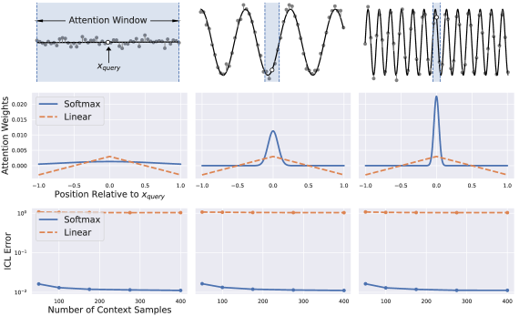
Figure 1: Top Row: The black line denotes the target function over a domain (horizontal axis). The gray dots are noisy training data, and the white dot is a query. From left to right, the Lipschitzness of the target function grows and the optimal softmax attention window (shaded blue) shrinks. Middle Row: Attention weights – which determine the attention window – as a function of the relative position from the query for softmax and linear attention. The softmax weights adjust to the Lipschitzness. Bottom Row: ICL error versus number of context samples for the three settings. Adapting to function Lipschitzness leads softmax attention to achieve small error. Please see Remark 2.1 and Appendix I for further discussion and details.

How does softmax attention learn to perform ICL?

There are two aspects to this question. (i) What does the attention unit learn from the pretraining tasks? and (ii) How does it use the pretraining to perform ICL? The architecture of the attention unit imposes a strong inductive bias, and it has been a challenge to interpret what aspect of the pretraining contexts translate to success during inference. To this end, we study a general function class, where the tasks only have shared Lipschitzness. Specifically, the rate at which their labels change along particular directions in the input space is similar across tasks. In such settings, we observe that (i) softmax attention adapts to the pretraining tasks by changing its attention window, i.e. the neighborhood of points around the query that strongly influence, or “attend to”, its prediction in accordance with this shared Lipschitzness and (ii) the attention unit uses this window to implement a nearest-neighbours type algorithm for inference. We also observe that this shared Lipschitzness is not only sufficient but necessary for ICL in some sense. Our main claim is as follows:

Main Claim: Softmax attention performs ICL by calibrating its attention window to the Lipschitzness of the pretraining tasks.

Technical Outline. We substantiate the above claim via two streams of analysis. To our knowledge, these are the first results showing that softmax attention pretrained on ICL tasks recovers shared structure among the tasks that facilitates ICL on downstream tasks.

(1) Attention window captures appropriate scale – Section 3. We prove that when the target function class belongs to one of two general families of linear and nonlinear function classes, the optimal weight matrix characterizing softmax attention scales with the Lipschitzness of the function class. We begin by showing that ICL for regression behaves as a nearest neighbours estimator using a learned attention window (Lemma B.5). We then develop novel concentrations for particular functionals on the distribution of the attention weights used by tokens distributed on the hypersphere (Corollary H.5). This begets tight upper and lower bounds on the ICL loss (Lemmas C.8 and C.9) for any window size, which we use to characterize the optimal window (Theorem 3.4). Further, we prove that pretrained softmax attention can in-context learn any downstream task with Lipschitzness similar to that of the pretraining tasks, and conversely that even changing only the Lipschitzness of the inference tasks results in degraded performance (Theorem 3.5) – implying learning Lipschitzness is both sufficient and necessary for generalization. To emphasize the importance of the softmax, we show that the minimum ICL loss achievable by linear attention on the aforementioned nonlinear family exceeds that achieved by pretrained softmax attention (Theorem 3.6).

(2) Attention window captures appropriate directions – Section 4. We prove that when the target function class consists of linear functions that share a common low-dimensional structure such that they only depend on the projection of the input onto a $k$-dimensional subspace, the optimal softmax attention weight matrix from pretraining projects the data onto this subspace (Theorem 4.4). In other words, softmax attention learns to zero-out the zero-Lipschitzness directions in the ambient data space, and thereby reduces the effective dimension of ICL. To show this, we prove that a particular gradient of the pretraining loss is always positive when the weight matrix has any component in the zero-Lipschitzness directions. The key to this is re-writing the expectation in the gradient as an integral of the sum of all four function values resulting from the four assignments of two particular tokens to two points on the hypersphere. Although the sum of function values resulting from subsets of these assignments may be negative, we show that the sum of all four function values is always positive for any two points (Lemmas G.3 and G.4).

Notations. We use (upper-, lower-)case boldface for (matrices, vectors), respectively. We denote the (identity, zero) matrix in $\mathbb{R}^{d\times d}$ as ($\mathbf{I}_{d}$, $\mathbf{0}_{d\times d}$), respectively, the set of column-orthonormal matrices in $\mathbb{R}^{d\times k}$ as $\mathbb{O}^{d\times k}$, and the (column space, 2-norm) of a matrix $\mathbf{B}$ as ($\operatorname{\text{col}}(\mathbf{B})$, $\|\mathbf{B}\|$), respectively. We indicate the unit hypersphere in $\mathbb{R}^{d}$ by $\mathbb{S}^{d-1}$ and the uniform distribution over $\mathbb{S}^{d-1}$ as $\mathcal{U}^{d}$. We use asymptotic notation ($\operatorname{\mathcal{O}}$, $\Omega$) to hide constants that depend only on the dimension $d$.

1.1 Additional Related Work

Numerous recent works have constructed transformers that can implement GD and other machine learning algorithms during ICL (von Oswald et al., 2023a; Akyürek et al., 2022; Bai et al., 2023; Fu et al., 2023a; Giannou et al., 2023), but it is unclear whether pretraining leads to such transformers. Li et al. (2023b) and Bai et al. (2023) provide generalization bounds for ICL via tools from algorithmic stability and uniform concentration, respectively. Wu et al. (2023) investigate the pretraining statistical complexity of learning a Bayes-optimal predictor for ICL on linear tasks with linear attention. Xie et al. (2021); Wang et al. (2023); Zhang et al. (2023) study the role of the pretraining data distribution, rather than the learning model, in facilitating ICL. Several have viewed softmax attention through the lens of kernel regression, but focused on either improving attention (Chen et al., 2023; Tsai et al., 2019; Nguyen et al., 2022; Han et al., 2022; Deng et al., 2023a) or analyzing the capability of a particular softmax-like kernel regressor to make Bayes-optimal predictions during ICL (Han et al., 2023), rather than studying what softmax attention actually learns during pretraining. There is a large body of additional work concerning training dynamics, expressivity, and other theoretical aspects of transformers, as well as empirical study of ICL; please see Appendix A for further discussion.

2 Preliminaries

In-Context Learning (ICL). Transformers have an astounding ability to adapt to novel contexts at inference time with no training. We study this phenomenon in the setting of regression. Specifically, in our model, each context consists of a set of feature vectors paired with scalar labels $\{\operatorname{{\bf\it x}}^{(t)}_{i},f_{t}(\operatorname{{\bf\it x}}^{(t)}_{i})\}$. The function $f_{t}$ used to label the features is drawn fresh for each context. During pretraining, the learner observes many such contexts to develop a pretrained model denoted by $\mathcal{A}(\{\{\operatorname{{\bf\it x}}^{(t)}_{i},f_{t}(\operatorname{{\bf\it x}}^{(t)}_{i})\}_{i}\}_{t})$. At inference time, a new context $f$ is drawn - new features and new labels $\{\operatorname{{\bf\it x}}_{i},f(\operatorname{{\bf\it x}}_{i})\}$, as well as one special feature vector - the query $\operatorname{{\bf\it x}}$. The ICL objective is to use the task information implicit in the labelings of the other features to correctly label the query $\mathcal{A}(\{\{\operatorname{{\bf\it x}}^{(t)}_{i},f_{t}(\operatorname{{\bf\it x}}^{(t)}_{i})\}_{i}\}_{t})(\operatorname{{\bf\it x}},\{\operatorname{{\bf\it x}}_{i},f(\operatorname{{\bf\it x}}_{i})\})\to f(\operatorname{{\bf\it x}})$. We emphasize that $\mathcal{A}$ is pretrained using $f_{1},f_{2},\cdots,f_{T}$ and tested on $f$. This deviates from the traditional machine learning paradigm of training on data $\operatorname{{\bf\it x}}_{1},\operatorname{{\bf\it x}}_{2},\cdots,\operatorname{{\bf\it x}}_{n}$ to predict $f(\operatorname{{\bf\it x}})$ for some fixed $f$. The difference is that ICL happens entirely in a forward pass, so there is no training on $f$. Our inquiry focuses on the role of the softmax activation in the self-attention unit that enables such inference. First, we discuss the details of the self-attention architecture.

The Softmax Self-Attention Unit. We consider a single softmax self-attention head $H_{SA}(\cdot;\boldsymbol{\theta}):\mathbb{R}^{(d+1)\times(n+1)}\rightarrow\mathbb{R}^{(d+1)\times(n+1)}$ parameterized by $\boldsymbol{\theta}\coloneqq\!(\mathbf{W}_{K},\mathbf{W}_{Q},\mathbf{W}_{V})$, where $\mathbf{W}_{K},\mathbf{W}_{Q},\mathbf{W}_{V}\in\mathbb{R}^{(d+1)\times(d+1)}$ are known as key, query, and value weight matrices, respectively. Intuitively, for a sequence of tokens $\mathbf{Z}=[\operatorname{{\bf\it z}}_{1},\dots,\operatorname{{\bf\it z}}_{n+1}]\in\operatorname{{\bf\it z}}^{(d+1)\times(n+1)}$, the attention layer creates a “hash map" where the key-value pairs come from key and value embeddings of the input tokens, $\{\operatorname{\mathbf{W}}_{K}\operatorname{{\bf\it z}}_{i}:\operatorname{\mathbf{W}}_{V}\operatorname{{\bf\it z}}_{i}\}$. Each token $\operatorname{{\bf\it z}}_{i}$ is interpreted as a query $\operatorname{\mathbf{W}}_{Q}\operatorname{{\bf\it z}}_{i}$, and during a pass through the attention layer, this query is matched with the keys $\{\operatorname{\mathbf{W}}_{K}\operatorname{{\bf\it z}}_{j}\}_{j}$ to return an average over the associated values $\{\operatorname{\mathbf{W}}_{V}\operatorname{{\bf\it z}}_{j}\}_{j}$ with a weight determined by the quality of the match (proportional to $e^{(\operatorname{\mathbf{W}}_{K}\operatorname{{\bf\it z}}_{j})^{\top}(\operatorname{\mathbf{W}}_{Q}\operatorname{{\bf\it z}}_{i})}$). Specifically, $H_{SA}(\mathbf{Z};\boldsymbol{\theta})=[h_{SA}(\mathbf{z}_{1},\mathbf{Z};\boldsymbol{\theta}),\cdots,h_{SA}(\mathbf{z}_{n+1},\mathbf{Z};\boldsymbol{\theta})]$, where

$$h_{SA}(\mathbf{z}_{i},\mathbf{Z};\boldsymbol{\theta})=\frac{\sum_{j=1}^{n}\left(\mathbf{W}_{V}\mathbf{z}_{j}\right)\;e^{(\mathbf{W}_{K}\mathbf{z}_{j})^{\top}(\mathbf{W}_{Q}\mathbf{z}_{i})}}{\sum_{i=1}^{n}e^{(\mathbf{W}_{K}\mathbf{z}_{j})^{\top}(\mathbf{W}_{Q}\mathbf{z}_{i})}}\in\mathbb{R}^{d+1}.$$ (ATTN)

With slight abuse of notation, we denote $h_{SA}(\mathbf{z}_{j})=h_{SA}(\mathbf{z}_{j},\mathbf{Z};\boldsymbol{\theta})$ when it is not ambiguous. To study how this architecture enables ICL, we follow Garg et al. (2022) to formalize ICL as a regression problem. Below we define the tokenization, pretraining objective and inference task.

Tokenization for regression. The learning model encounters token sequences of the form

$$\mathbf{Z}:=\begin{bmatrix}\operatorname{{\bf\it x}}_{1}&\operatorname{{\bf\it x}}_{2}&\ldots&\operatorname{{\bf\it x}}_{n}&\operatorname{{\bf\it x}}_{n+1}\\ f(\operatorname{{\bf\it x}}_{1})+\epsilon_{1}&f(\operatorname{{\bf\it x}}_{2})+\epsilon_{1}&\ldots&f(\operatorname{{\bf\it x}}_{n})+\epsilon_{n}&0\\ \end{bmatrix}\in\mathbb{R}^{(d+1)\times(n+1)},$$ (1)

where the ground-truth labelling function $f$ maps from $\mathbb{R}^{d}$ to $\mathbb{R}$ and belongs to some class $\mathcal{F}$, each $\epsilon_{i}$ is mean-zero noise, and the $i$-th input feature vector $\operatorname{{\bf\it x}}_{i}\in\mathbb{R}^{d}$ is jointly embedded in the same token with its noisy label $f(\operatorname{{\bf\it x}}_{i})+\epsilon_{i}\in\mathbb{R}$. We denote this token $\mathbf{z}_{i}$. The ICL task is to accurately predict this label given the $n$ context tokens $\{(\operatorname{{\bf\it x}}_{i},f(\operatorname{{\bf\it x}}_{i})+\epsilon_{i})\}_{i=1}^{n}$, where $f$ may vary across sequences. The prediction for the label of the $(n\!+\!1)$-th feature vector is the $(d\!+\!1)$-th element of $h_{SA}(\mathbf{z}_{n+1})$ (Cheng et al., 2023), denoted $h_{SA}(\mathbf{z}_{n+1})_{d+1}$. Ultimately, the goal is to learn weight matrices such that $h_{SA}(\mathbf{z}_{n+1})_{d+1}$ is likely to approximate the $(n+1)$-th label on a random sequence $\mathbf{Z}$.

Pretraining protocol. We study what softmax attention learns when its weight matrices are pretrained using sequences of the form of (1). These sequences are randomly generated as follows:

$$f\sim D(\mathcal{F}),\quad\operatorname{{\bf\it x}}_{1},\dots,\operatorname{{\bf\it x}}_{n+1}\stackrel{{\scriptstyle\text{i.i.d.}}}{{\sim}}D_{\operatorname{{\bf\it x}}}^{\otimes(n+1)},\quad\epsilon_{1},\dots,\epsilon_{n}\stackrel{{\scriptstyle\text{i.i.d.}}}{{\sim}}D_{\epsilon}^{\otimes(n+1)}$$ (2)

where $D(\mathcal{F})$ is a distribution over functions in $\mathcal{F}$, $D_{\operatorname{{\bf\it x}}}$ is a distribution over $\mathbb{R}^{d}$, and $D_{\epsilon}$ is a distribution over $\mathbb{R}$ with mean zero and variance $\sigma^{2}$. The token embedding sequence $\mathbf{Z}$ is then constructed as in (1). Given this generative model, the pretraining loss of the parameters $\boldsymbol{\theta}=(\mathbf{W}_{Q},\mathbf{W}_{K},\mathbf{W}_{V})$ is the expected squared difference between the prediction of softmax attention and the ground-truth label of the $(n\!+\!1)$-th input feature vector in each sequence, namely

$$\bar{\operatorname{\mathcal{L}}}(\boldsymbol{\theta}):=\operatorname{\mathbb{E}}_{f,\{\operatorname{{\bf\it x}}_{i}\}_{i},\{\epsilon_{i}\}_{i}}\left(h_{SA}(\mathbf{z}_{n+1})_{d+1}-f(\operatorname{{\bf\it x}}_{n+1})\right)^{2}.$$ (3)

We next reparameterize the attention weights to make (3) more interpretable. First, note that this loss is not a function of the first $n$ columns of $\mathbf{W}_{V}$, so without loss of generality, we set them to zero. For the last column, we show in Appendix B that any minimizer of (3) in the settings we consider must have the first $d$ elements of this last column equal to zero. As in Cheng et al. (2023), we fix the $(d\!+\!1,d\!+\!1)$-th element of $\mathbf{W}_{V}$, here as 1 for simplicity. In the same vein, we follow Ahn et al. (2023); Cheng et al. (2023) by setting the $(d\!+\!1)$-th row and column of $\mathbf{W}_{K}$ and $\mathbf{W}_{Q}$ equal to zero. To summarize, the reparameterized weights are:

$$\mathbf{W}_{V}=\begin{bmatrix}\mathbf{0}_{d\times d}&\mathbf{0}_{d\times 1}\\ \mathbf{0}_{1\times d}&1\\ \end{bmatrix},\quad\mathbf{W}_{K}=\begin{bmatrix}\mathbf{M}_{K}&\mathbf{0}_{d\times 1}\\ \mathbf{0}_{1\times d}&0\\ \end{bmatrix},\quad\mathbf{W}_{Q}=\begin{bmatrix}\mathbf{M}_{Q}&\mathbf{0}_{d\times 1}\\ \mathbf{0}_{1\times d}&0\\ \end{bmatrix}$$ (4)

where $\mathbf{M}_{K},\mathbf{M}_{Q}\in\mathbb{R}^{d\times d}$. Now, since our goal is to reveal properties of minimizers of the pretraining loss, rather than study the dynamics of optimizing the loss, without loss of generality we can define $\mathbf{M}:=\mathbf{M}_{K}^{\top}\mathbf{M}_{Q}$ and re-define the pretraining loss (3) as a function of $\mathbf{M}$. Doing so yields:

$$\operatorname{\mathcal{L}}(\mathbf{M}):=\operatorname{\mathbb{E}}_{f,\{\operatorname{{\bf\it x}}_{i}\}_{i},\{\epsilon_{i}\}_{i}}\left(\frac{\sum_{i=1}^{n}(f(\operatorname{{\bf\it x}}_{i})+\epsilon_{i})\;e^{\operatorname{{\bf\it x}}_{i}^{\top}\mathbf{M}\operatorname{{\bf\it x}}_{n+1}}}{\sum_{i=1}^{n}e^{\operatorname{{\bf\it x}}_{i}^{\top}\mathbf{M}\operatorname{{\bf\it x}}_{n+1}}}-f(\operatorname{{\bf\it x}}_{n+1})\right)^{2}.\vspace{1mm}$$ (ICL)

Interpretation of the pretraining loss. The loss (ICL) clarifies how softmax attention can be interpreted as a nearest neighbors regressor. Under the assumption that $\operatorname{{\bf\it x}}_{i}^{\top}\mathbf{M}\operatorname{{\bf\it x}}_{n+1}$ is a proxy for the distance between $\operatorname{{\bf\it x}}_{i}$ and $\operatorname{{\bf\it x}}_{n+1}$ (which we formally show in Section 3), the softmax attention prediction is a convex combination of the noisy labels with weights determined by the closeness of $\operatorname{{\bf\it x}}_{i}$ to $\operatorname{{\bf\it x}}_{n+1}$, such that the labels of points closer to $\operatorname{{\bf\it x}}_{n+1}$ have larger weight. Moreover, the decay in weights on points further from $\operatorname{{\bf\it x}}_{n+1}$ is exponential and controlled by $\mathbf{M}$, which effectively defines a neighborhood, or attention window, of points around $\operatorname{{\bf\it x}}_{n+1}$ whose labels have non-trivial weight. More formally, we can think of the attention window defined for a query $\operatorname{{\bf\it x}}_{n+1}$ as the set $\texttt{AttnWindow}(\operatorname{{\bf\it x}}_{n+1};\mathbf{M}):=\{\operatorname{{\bf\it x}}:\operatorname{{\bf\it x}}^{\top}\mathbf{M}\operatorname{{\bf\it x}}_{n+1}=\Omega(1)\}$. As we have observed in Figure 1, our key insight is that pretrained $\mathbf{M}$ scales this attention window with the Lipschitzness of the function class. Generally speaking, larger $\mathbf{M}$ entails averaging over a smaller window and incurring less bias due to the function values of distant tokens in the estimate, while smaller $\mathbf{M}$ entails averaging over a larger window, resulting in larger bias due to distant token labels, but a smaller noise variance. Figure 2 further depicts this tradeoff.

Remark 2.1 (Extreme cases and the softmax advantage).

Consider the following two settings.

Constant functions. If each of the functions the attention unit sees in pretraining is constant, as in the Left column of Figure 1, it is best to consider an infinite attention window, that is, take $\mathbf{M}=\mathbf{0}_{d\times d}$ as this results in a uniform average over all the noisy token labels.

Rapidly changing functions. If the pretraining functions change rapidly, as in the Right column of Figure 1, attending to a distant token might serve only to corrupt the estimate at the target. Consider another example in which the input tokens are used to construct Voronoi cells on the surface of the hypersphere and the label for a new token in a cell is the label of the token used to construct that cell, where labels across cells may vary arbitrarily. The optimal estimator would attend only to the single nearest token since this incurs error only from label noise. In other words, we would choose $\mathbf{M}=\infty\mathbf{I}_{d}$.

Advantage of the softmax. To further highlight the property of softmax that enables the behaviour discussed above, we compare with linear attention (von Oswald et al., 2023a; Zhang et al., 2023; Ahn et al., 2023), whose estimator can be written as $h_{LA}(\operatorname{{\bf\it x}})=\sum_{i}(f(\operatorname{{\bf\it x}}_{i})+\epsilon_{i})\operatorname{{\bf\it x}}_{i}^{\top}\mathbf{M}\operatorname{{\bf\it x}}$, up to a universal scaling due to the value embedding. This is again a weighted combination of labels, but one that does not allow for adapting an attention window – any scaling of $\mathbf{M}$ does not change the relative weights placed on each label – unlike softmax attention. Please see Figure 1 (Middle Row) for a comparison of the weights used in the different estimators.

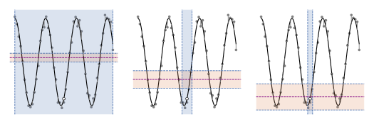
Figure 2: From left to right, as we shrink the attention window (shaded in blue shading), the estimator has lower bias (shown in purple) but larger variance (shaded in tan).

3 Pretraining Learns Scale of Attention Window

One of our observations of the estimator used by attention, $h_{SA}$ (defined in Equation ATTN) is that it computes a nearest neighbours regression. We hypothesize that the role of pretraining is to select a neighbourhood within which to select tokens for use in the estimator. In this section we characterize this size. First, we define function Lipschitzness and the families of function classes we study.

Definition 3.1 (Lipschitzness).

A function $f:\mathcal{X}\rightarrow\mathbb{R}$ has Lipschitzness $L$ if $L$ is the smallest number satisfying $f(\operatorname{{\bf\it x}})-f(\operatorname{{\bf\it x}}^{\prime})\leq L\|\operatorname{{\bf\it x}}-\operatorname{{\bf\it x}}^{\prime}\|$ for all $(\operatorname{{\bf\it x}},\operatorname{{\bf\it x}}^{\prime})\in\mathcal{X}^{2}$.

Definition 3.2 (Affine and ReLU Function Classes).

The function classes $\mathcal{F}^{\text{aff}}_{L}$ and $\mathcal{F}^{+}_{L}$ are respectively defined as:

$$\mathcal{F}^{\text{aff}}_{L} :=\{f:f(\operatorname{{\bf\it x}})=l\;\mathbf{w}^{\top}\operatorname{{\bf\it x}}+\ b,\;\mathbf{w}\in\mathbb{S}^{d-1},b,l\in[-L,L]\},$$

$$\mathcal{F}^{+}_{L} :=\{f:f(\operatorname{{\bf\it x}})=l_{1}(\mathbf{w}^{\top}\operatorname{{\bf\it x}})_{+}+l_{2}(-\mathbf{w}^{\top}\operatorname{{\bf\it x}})_{+}+b,\;\mathbf{w}\in\mathbb{S}^{d-1},(b,l_{1},l_{2})\in[-L,L]^{2}\}.$$

$D(\operatorname{\mathcal{F}}^{\text{aff}}_{L}),D(\mathcal{F}^{+}_{L})$ are induced by drawing $\mathbf{w}\sim\mathcal{U}^{d}$ and $b,l,l_{1},l_{2}\stackrel{{\scriptstyle\text{i.i.d.}}}{{\sim}}\text{Unif}([-L,L])$. We say that these classes are $L-$Lipschitz, as the maximum Lipschitzness of any function in the class is $L$.

Here, $(z)_{+}:=\max(z,0)$. Next, we assume the covariates are uniform on the hypersphere.

Assumption 3.3 (Covariate Distribution).

The covariate distribution $D_{\operatorname{{\bf\it x}}}=\mathcal{U}^{d}$.

Now we are ready to state our main theorem.

Theorem 3.4.

Consider the pretraining loss (ICL) in the cases wherein Assumption 3.3 holds and tasks $f$ are drawn from (Case 1) $D(\mathcal{F}^{\text{aff}}_{L})$ or (Case 2) $D(\mathcal{F}^{+}_{L})$. For $n=\Omega(1)$ and $\Omega(n^{-d/2})\leq\sigma^{2}\leq\mathcal{O}(nL^{2})$, any minimizer $\mathbf{M}^{*}$ of (ICL) satisfies $\mathbf{M}^{*}=w_{KQ}\mathbf{I}_{d}$ , where for $\Lambda\coloneqq\frac{nL^{2}}{\sigma^{2}}$, $\alpha\coloneqq\frac{1}{d+4}$ and $\beta\coloneqq\frac{1}{d+2}$:

(Case 1) $$\;\;\Omega\left(\Lambda^{\alpha}\right)\leq w_{KQ}\leq\mathcal{O}\left(\Lambda^{\frac{2\alpha}{1-\beta}}\right),\quad\textbf{(Case 2)}\;\;\Omega\left(\Lambda^{\beta}\right)\leq|w_{KQ}|\leq\mathcal{O}\left(\Lambda^{2\beta}\right).$$

Theorem 3.4 shows that optimizing the pretraining population loss in Equation ICL leads to attention key-query parameters that scale with the Lipschitzness of the function class, as well as the noise level and number of in-context samples. These bounds align with our observations from Figures 1 and 2 that softmax attention selects an attention window that shrinks with the function class Lipschitzness, recalling that larger $w_{KQ}$ results in a smaller window. Further, the dependencies of the bounds on $\sigma^{2}$ and $n$ are also intuitive, since larger noise should encourage wider averaging to average out the noise, and larger $n$ should encourage a smaller window since more samples makes it more likely that there are samples very close to the query. To our knowledge, this is the first result showing that softmax attention learns properties of the task distribution during pretraining that facilitate ICL. Further, we have the following consequence for general inference tasks.

Theorem 3.5.

Suppose softmax attention is first pretrained on tasks drawn from $D(\operatorname{\mathcal{F}}_{L}^{+})$ and then tested on an arbitrary $L-$Lipschitz task, then the loss on the new task is upper bounded as $\operatorname{\mathcal{L}}\leq\operatorname{\mathcal{O}}(\frac{L^{2}}{\Lambda^{\beta}}).$ Furthermore, if the new task is instead drawn from $D(\operatorname{\mathcal{F}}_{L^{\prime}}^{+})$, the loss is lower bounded as $\operatorname{\mathcal{L}}\geq\Omega(\frac{L^{\prime 2}}{\Lambda^{2\beta}})$ for $L^{\prime}>L$ and $\operatorname{\mathcal{L}}\geq\Omega(\frac{\Lambda^{\beta d/2}}{n})$ for $L^{\prime}<L$.

Theorem 3.5 shows that pretraining on $D(\operatorname{\mathcal{F}}_{L}^{+})$ yields a model that can perform ICL on downstream tasks if and only if they have similar Lipschitzness as $L$. Thus, learning Lipschitzness is both sufficient and necessary for ICL. If the Lipschitzness of the tasks seen during inference are much larger than those seen in pretraining, we will end up with biased estimates. On the other hand, if the Lipschitzness during inference is much lower, we are not optimally averaging the noise. Please see Appendix E.1 for the proof.

3.1 Proof Sketch

To highlight the key insights of our analysis, in this section we consider a modification of the softmax attention that exhibits important properties of the original. Note that this approximation is for illustration only; the above results use the original softmax attention – see Appendices C, D, E. For now, consider a function class $\operatorname{\mathcal{F}}_{L}:=\{f:f(\operatorname{{\bf\it x}})=L\mathbf{w}^{\top}\operatorname{{\bf\it x}},\;\mathbf{w}\in\mathbb{S}^{d-1}\}$ of linear functions.

(Temporary) modification of the softmax attention. Rather than averaging over every token with a weight that decays exponentially with distance, we consider a modification which uniformly averages all tokens within a distance specified by $w_{KQ}=\|\mathbf{M}\|$. From Lemma B.5, without loss of generality (WLOG) we can consider $\mathbf{M}=w_{KQ}\mathbf{I}_{d}$. This means that, ignoring normalization, the weight assigned to $f(\operatorname{{\bf\it x}}_{i})$ by the true soft-max attention is $e^{-w_{KQ}\|\operatorname{{\bf\it x}}-\operatorname{{\bf\it x}}_{i}\|^{2}}$. That is, for all $\operatorname{{\bf\it x}}_{i}$ satisfying $\|\operatorname{{\bf\it x}}-\operatorname{{\bf\it x}}_{i}\|<\nicefrac{{1}}{{\sqrt{w_{KQ}}}}$, the assigned weights are all $\Theta(1)$, specifically in $(e^{-1},1]$. Meanwhile, for $\operatorname{{\bf\it x}}_{i}$ satisfying $\|\operatorname{{\bf\it x}}-\operatorname{{\bf\it x}}_{i}\|=\nicefrac{{\sqrt{c}}}{{\sqrt{w_{KQ}}}}$ for $c>1$, the weights are $e^{-c}$, decaying exponentially in $c$. This motivates us to consider a “modified softmax attention" given by $h_{MSA}(\operatorname{{\bf\it x}}):=\sum_{i}\frac{f(\operatorname{{\bf\it x}}_{i})\mathbbm{1}_{i}}{\sum_{j}\mathbbm{1}_{j}},$ where $\mathbbm{1}_{j}:=\mathbbm{1}\{\|\operatorname{{\bf\it x}}-\operatorname{{\bf\it x}}_{j}\|<\nicefrac{{1}}{{\sqrt{w_{KQ}}}}\}$. In particular, $h_{MSA}(\operatorname{{\bf\it x}})$ uniformly averages the labels of points within a Euclidean ball of radius $\nicefrac{{1}}{{\sqrt{w_{KQ}}}}$ around $\operatorname{{\bf\it x}}$, and ignores all others.

The In-Context Loss. Since the (label) noise is independent of all other random variables, the pretraining loss from Equation ICL can be decomposed into distinct weighted sums of labels and noise:

$$\operatorname{\mathcal{L}}(w_{KQ}\mathbf{I}_{d})=\underbrace{\operatorname{\mathbb{E}}_{f,\{\operatorname{{\bf\it x}}_{i}\}_{i}}\left(\sum_{j}\frac{(f(\operatorname{{\bf\it x}}_{n+1})-f(\operatorname{{\bf\it x}}_{j}))\mathbbm{1}_{j}}{\sum_{j}\mathbbm{1}_{j}}\right)^{2}}_{=:\operatorname{\mathcal{L}_{\text{signal}}}(w_{KQ})}+\underbrace{\operatorname{\mathbb{E}}_{\{\operatorname{{\bf\it x}}_{i}\}_{i},\{\epsilon_{i}\}_{i}}\left(\sum_{i}\frac{\epsilon_{i}\mathbbm{1}_{i}}{\sum_{j}\mathbbm{1}_{j}}\right)^{2}}_{=:\operatorname{\mathcal{L}_{\text{noise}}}(w_{KQ})}.$$

We first upper and lower bound each of these terms separately, starting with $\operatorname{\mathcal{L}_{\text{signal}}}(w_{KQ})$.

Noiseless Estimator Bias. (Please see Appendix C) This term is the squared difference between an unweighted average of the token labels within a radius of $\operatorname{{\bf\it x}}$, and the true label. Take $w_{KQ}=\Omega(1)$. Then for large $d$, most of the points $\operatorname{{\bf\it x}}_{i}$ satisfying $\|\operatorname{{\bf\it x}}-\operatorname{{\bf\it x}}_{i}\|\leq\nicefrac{{1}}{{\sqrt{w_{KQ}}}}$ lie on the boundary of the cap, that is, $\|\operatorname{{\bf\it x}}-\operatorname{{\bf\it x}}_{i}\|<\nicefrac{{1}}{{\sqrt{w_{KQ}}}}\implies\|\operatorname{{\bf\it x}}-\operatorname{{\bf\it x}}_{i}\|\approx\nicefrac{{1}}{{\sqrt{w_{KQ}}}}.$ This motivates us to approximate the set of points $\operatorname{{\bf\it x}}_{i}$ satisfying the above as coming from a uniform distribution over just the boundary of the cap. The center of mass of a ring of radius $\nicefrac{{1}}{{\sqrt{w_{KQ}}}}$ embedded on the surface of a hyper-sphere, is $\operatorname{\mathcal{O}}(\nicefrac{{1}}{{w_{KQ}}})$ from the boundary of a sphere, so the squared bias is $\Theta(\nicefrac{{L^{2}}}{{w^{2}_{KQ}}})$.

Noise. (Please see Appendix D for details) Since the noise is independent across tokens, expanding the square reveals that $\mathcal{L}_{\text{noise}}(w_{KQ})=\frac{\sigma^{2}}{\sum_{j}\mathbbm{1}_{j}}$, which is proportional to the reciprocal of the number of tokens found within a $\nicefrac{{1}}{{\sqrt{w_{KQ}}}}$ radius of $\operatorname{{\bf\it x}}$. In Lemma H.1, we derive bounds for the measure in this region and for now we ignore any finite-sample effects and replace the sum in the denominator with its expectation. This allows us to bound $\frac{1}{\sum_{j}\mathbbm{1}_{j}}=\Theta\big{(}\nicefrac{{w_{KQ}^{\frac{d}{2}}}}{{n}}\big{)}$ as long as $w_{KQ}\lesssim n^{2/d}$.

Combining the $\operatorname{\mathcal{L}_{\text{signal}}}$ and $\operatorname{\mathcal{L}_{\text{noise}}}$ terms. (Please see Appendix E for details) Overall, we have $\operatorname{\mathcal{L}}=\operatorname{\mathcal{L}_{\text{signal}}}+\operatorname{\mathcal{L}_{\text{noise}}}$ with $\operatorname{\mathcal{L}_{\text{signal}}}=\Theta\big{(}\nicefrac{{L^{2}}}{{w_{KQ}}}\big{)}$ and $\operatorname{\mathcal{L}_{\text{noise}}}=\Theta\big{(}\nicefrac{{w_{KQ}^{\frac{d}{2}}\sigma^{2}}}{{n}}\big{)}$. Minimizing this sum reveals that the optimal $w_{KQ}$ satisfies $w_{KQ}=\Theta\big{(}(\nicefrac{{nL^{2}}}{{\sigma^{2}}})^{\frac{2}{d+2}}\big{)}$.

3.2 Necessity of Softmax

To further emphasize the importance of the softmax in Theorem 3.4, we next study the performance of an analogous model with the softmax removed. We consider linear self-attention (von Oswald et al., 2023a; Zhang et al., 2023; Ahn et al., 2023), which replaces the softmax activation with an identity operation. In particular, in the in-context regression setting we study, the prediction of $f(\operatorname{{\bf\it x}}_{n+1})$ by linear attention and the corresponding pretraining loss are given by:

$$h_{LA}(\operatorname{{\bf\it x}}_{n+1}):=\sum_{i=1}^{n}(f(\operatorname{{\bf\it x}}_{i})+\epsilon_{i}){\operatorname{{\bf\it x}}_{i}^{\top}\mathbf{M}\operatorname{{\bf\it x}}_{n+1}},\;\;\mathcal{L}_{\text{LA}}(\mathbf{M}):=\operatorname{\mathbb{E}}_{f,\{\operatorname{{\bf\it x}}_{i}\}_{i},\{\epsilon_{i}\}_{i}}\left(h_{LA}(\operatorname{{\bf\it x}}_{n+1})-f(\operatorname{{\bf\it x}}_{n+1})\right)^{2}.$$

As discussed in Remark 2.1, $h_{LA}(\operatorname{{\bf\it x}}_{n+1})$ cannot adapt an attention window to the problem setting. We show below that this leads it to large ICL loss when tasks are drawn from $D(\mathcal{F}_{L}^{+})$.

Theorem 3.6 (Lower Bound for Linear Attention).

Consider pretraining on $\mathcal{L}_{\text{LA}}$ with tasks $f$ drawn from $D(\mathcal{F}^{+}_{L})$ and covariates drawn from $\mathcal{U}^{d}$. Then for all $\mathbf{M}\in\mathbb{R}^{d\times d}$, $\mathcal{L}_{LA}(\mathbf{M})=\Omega({L^{2}})$.

This lower bound on $\mathcal{L}_{LA}$ is strictly larger than the upper bound on $\mathcal{L}$ from Theorem 3.5, up to factors in $d$, as long as $\frac{\sigma^{2}}{n}\leq 1$, which holds in all reasonable cases. Please see Appendix F for the proof.

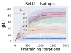
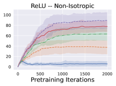
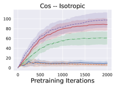
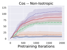
Figure 3: Spectral norm of $\mathbf{M}$ during pretraining with varying $L$. Each plot shows results for different task and covariate distributions, with (tasks, covariates) drawn from (Left) ($D(\mathcal{F}_{L}^{+}),\mathcal{U}^{d}$), (Middle-Left) ($D(\mathcal{F}_{L}^{+}),\tilde{\mathcal{U}}^{d}$), (Middle-Right) ($D(\mathcal{F}_{L}^{\cos}),\mathcal{U}^{d}$), (Right) ($D(\mathcal{F}_{L}^{\cos}),\tilde{\mathcal{U}}^{d}$), where $\tilde{\mathcal{U}}^{d}$ is a non-isotropic distribution on $\mathbb{S}^{d-1}$ (see Section 3.3 for its definition).

3.3 Experiments

We next empirically verify our intuitions and results regarding learning the scale of the attention window. In all cases we train $\mathbf{M}_{K}$ and $\mathbf{M}_{Q}$ with Adam with one task sampled per round, use the noise distribution $D_{\epsilon}=\mathcal{N}(0,\sigma^{2})$, and run $10$ trials and plot means and standard deviations over these 10 trials. Please see Appendix I for full details as well as additional results.

Ablations over $L$, $\sigma$ and $n$. We first verify whether the relationship between the attention window scale – i.e. $\|\mathbf{M}\|^{-1}$ – and $L$, $\sigma$ and $n$ matches our bounds in Theorem 3.4 for the case when tasks are drawn from $D(\mathcal{F}^{+}_{L})$ and the covariates are drawn from $\mathcal{U}^{d}$, as well as whether these relationships generalize to additional function classes and covariate distributions. To do so, we train on tasks drawn from $D(\mathcal{F}^{+}_{L})$ and $D(\mathcal{F}^{\cos}_{L})$, where $\mathcal{F}^{\cos}_{L}:=\{f:f(\operatorname{{\bf\it x}})=\cos(L\mathbf{w}^{\top}\operatorname{{\bf\it x}}),\;\mathbf{w}\in\mathbb{S}^{d-1}\}$ and $D(\mathcal{F}^{\cos}_{L})$ is induced by sampling $\mathbf{w}\sim\mathcal{U}^{d}$. In all cases we set $d=5$, and use $(L,\sigma,n)=(1,0.01,20)$ if not ablating over these parameters, and vary only one of $\{L,\sigma,n\}$ and no other hyperparameters within each plot.

Attention window scales inversely with $L$. Figure 3 shows that $\|\mathbf{M}\|$ indeed increases with $L$ in various settings. In Figure 3(Left, Middle-Left), tasks are drawn from $D(\mathcal{F}^{+}_{L})$, and in Figure 3(Middle-Right, Right), they are drawn $D(\mathcal{F}^{\cos}_{L})$. In Figure 3(Left, Middle-Right), each $\operatorname{{\bf\it x}}_{i}$ is drawn from $\mathcal{U}^{d}$, whereas in Figure 3(Middle-Left, Right), each $\operatorname{{\bf\it x}}_{i}$ is drawn from a non-isotropic distribution $\tilde{\mathcal{U}}^{d}$ on $\mathbb{S}^{d-1}$ defined as follows. First, let $\mathbf{S}_{d}:=\text{diag}([1,\dots,d])\in\mathbb{R}^{d\times d}$, then $\operatorname{{\bf\it x}}\sim\tilde{\mathcal{U}}^{d}$ is generated by sampling $\hat{\operatorname{{\bf\it x}}}\sim\mathcal{N}(\mathbf{0}_{d},\mathbf{I}_{d})$, then computing $\operatorname{{\bf\it x}}=\frac{\mathbf{S}_{d}^{1/2}\hat{\operatorname{{\bf\it x}}}}{\|\mathbf{S}_{d}^{1/2}\hat{\operatorname{{\bf\it x}}}\|_{2}}$. Note that although larger $L$ implies larger $\|\nabla_{\mathbf{x}}f(\operatorname{{\bf\it x}})\|$ on average across $f$, it is not immediately clear that it implies larger $\|\nabla_{\mathbf{M}_{K}}\mathcal{L}(\mathbf{W}_{K}^{\top}\mathbf{W}_{Q})\|$ nor $\|\nabla_{\mathbf{M}_{Q}}\mathcal{L}(\mathbf{W}_{K}^{\top}\mathbf{W}_{Q})\|$, so in this sense it is surprising that larger $L$ implies larger pretrained $\mathbf{M}$ (although it is consistent with our intuition and results).

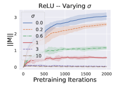
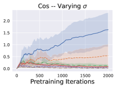
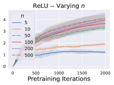
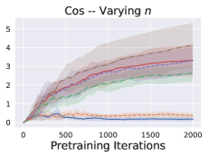
Figure 4: Spectral norm of $\mathbf{M}$ during pretraining on tasks drawn from $D(\mathcal{F}^{+}_{1})$ in Left, Middle-Right and $D(\mathcal{F}^{\cos}_{1})$ in Middle-Left, Right. Left, Middle-Left show ablations over the noise standard deviation $\sigma$ and Middle-Right, Right show ablations over the number of context samples $n$.

Attention window scales with $\sigma$, inversely with $n$. Figure 4 shows that the dependence of $\|\mathbf{M}\|$ on $\sigma$ and $n$ also aligns with Theorem 3.4. As expected, $\|\mathbf{M}\|$ increases slower during pretraining for larger $\sigma$ (shown in Figures 4(Left, Middle-Left)), since more noise encourages more averaging over a larger window to cancel out the noise. Likewise, $\|\mathbf{M}\|$ increases faster during pretraining for larger $n$ (shown in Figures 4(Middle-Right, Right)), since larger $n$ increases the likelihood that there is a highly informative sample within a small attention window. Here the covariate distribution is $\mathcal{U}^{d}$ in all cases.

Learning new tasks in-context. An important implication of our analysis is that for the function classes we consider, the softmax attention estimator does not adapt to the function class beyond its Lipschitzness. We have already seen in Figures 3 and 4 that the growth of $\|\mathbf{M}\|$ during pretraining is similar across different function classes with the same Lipschitzness, as long as $\sigma$ and $n$ are fixed. Here we verify the conclusion from Theorem 3.5 that for fixed $n$ and $\sigma$, the necessary and sufficient condition for downstream generalization, measured by small ICL error, is that the pretraining and downstream tasks have similar Lipschitzness. Figure 5 supports this conclusion. Here we set $d=5,n=200,\sigma=0.01$ and draw each $\operatorname{{\bf\it x}}_{i}$ i.i.d. from $\mathcal{U}^{d}$. In Figure 5(Left, Middle-Left, Middle-Right), we train three attention units on tasks drawn from the 1-Lipschitz affine ($D(\operatorname{\mathcal{F}}_{1}^{\text{aff}})$), ReLU ($D(\operatorname{\mathcal{F}}_{1}^{+})$), and cosine ($D(\operatorname{\mathcal{F}}_{1}^{\cos})$) task distributions, respectively. Each plot shows the test ICL error on tasks drawn from a particular distribution among $\{D(\operatorname{\mathcal{F}}_{1}^{\text{aff}}),D(\operatorname{\mathcal{F}}_{1}^{+}),D(\operatorname{\mathcal{F}}_{1}^{\cos})$}. Performance is similar regardless of the pairing of pretraining and test distributions, as the Lipschitzness is the same in all cases, demonstrating that pretraining on tasks with appropriate Lipschitzness is sufficient for generalization.

Moreover, Figure 5(Right) shows that when the Lipschitzness of the pretraining tasks does not match that of the test tasks, ICL performance degrades sharply, even when the tasks otherwise share similar structure. Here the test task distribution is $D(\mathcal{F}_{1}^{\cos})$, and the pretraining task distributions are $D(\mathcal{F}_{1}^{\text{aff}})$, $D(\mathcal{F}_{0.1}^{\text{cos}})$, and $D(\mathcal{F}_{10}^{\text{cos}})$. The only pretraining distribution that leads to downstream generalization is $D(\mathcal{F}_{1}^{\text{aff}})$ since its Lipschitzness matches that of the downstream tasks, despite the fact that it is not a distribution over cosine functions, unlike the other distributions. Thus, these results lend credence to the idea that in addition to being sufficient, pretraining on tasks with appropriate Lipschitzness is necessary for generalization.

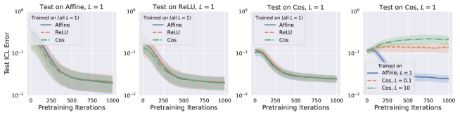
Figure 5: Left, Middle-Left, Middle-Right: The test ICL error for softmax attention as it is trained on the distributions over the 1-Lipschitz affine, ReLU, and cosine function classes ($D(\mathcal{F}^{\text{aff}}_{1})$, $D(\mathcal{F}^{+}_{1})$, and $D(\mathcal{F}^{\cos}_{1})$, respectively), where the ICL error is evaluated at each pretraining iteration on 5 tasks drawn from the distributions over the 1-Lipschitz (affine, ReLU, cosine) function classes in (Left, Middle-Left, Middle-Right), respectively. Right: The test ICL error evaluated on tasks drawn from $D(\mathcal{F}^{\cos}_{1})$ for three softmax attention units trained on tasks drawn from $D(\mathcal{F}^{\text{aff}}_{1})$, $D(\mathcal{F}^{\cos}_{0.1})$, and $D(\mathcal{F}^{\cos}_{10})$, respectively.

4 Softmax Attention Learns Direction of Attention Window

Thus far, we have considered distributions over tasks that treat the value of the input data in all directions within the ambient space as equally relevant to its label. However, in practice the ambient dimension of the input data is often much larger than its information content – the labels may change very little with many features of the data, meaning that such features are spurious. This is generally true of embedded language tokens, whose embedding dimension is typically far larger than the minimum dimension required to store them (logarithmic in the vocabulary size) (Brown et al., 2020). Motivated by this, we define a notion of “direction-wise Lipschitzness” of a function class to allow for analyzing classes that may depend on some directions within the ambient input data space more than others.

Definition 4.1 (Direction-wise Lipschitzness of Function Class).

The Lipschitzness of a function class $\mathcal{F}$ with domain $\mathcal{X}\subseteq\mathbb{R}^{d}$ in the direction $\mathbf{w}\in\mathbb{S}^{d-1}$ is defined as as the largest Lipschitz constant of all functions in $\mathcal{F}$ over the domain $\mathcal{X}$ projected onto $\mathbf{w}$, that is:

$$\operatorname{\text{Lip}}_{\mathbf{w}}(\mathcal{F},\mathcal{X}):=\inf_{L\in\mathbb{R}}\{ L:f(\mathbf{ww}^{\top}\operatorname{{\bf\it x}})-f(\mathbf{ww}^{\top}\operatorname{{\bf\it x}}^{\prime})\leq L|\mathbf{w}^{\top}\operatorname{{\bf\it x}}-\mathbf{w}^{\top}\operatorname{{\bf\it x}}^{\prime}|\;\;\forall\;(\operatorname{{\bf\it x}},\operatorname{{\bf\it x}}^{\prime})\in\mathcal{X}^{2},f\in\mathcal{F}\}.$$

Using this definition, we analyze function classes consisting of linear functions with parameters lying in a subspace of $\mathbb{R}^{d}$, as follows:

Definition 4.2 (Low-rank Linear Function Class).

The function class $\mathcal{F}^{\text{lin}}_{\mathbf{B}}$ is defined as $\mathcal{F}^{\text{lin}}_{\mathbf{B}}:=\{{f}:{f}(\operatorname{{\bf\it x}})=\mathbf{a}^{\top}\mathbf{B}^{\top}\operatorname{{\bf\it x}},\;\mathbf{a}\in\mathbb{R}^{k}\}$, and $D(\operatorname{\mathcal{F}}^{\text{lin}}_{\mathbf{B}})$ is induced by drawing $\mathbf{a}\sim\mathcal{U}^{k}$.

where $\mathbf{B}\in\mathbb{O}^{d\times k}$ is a column-wise orthonormal matrix. Since our motivation is settings with low-dimensional structure, we can think of $k\ll d$. Let $\mathbf{B}_{\perp}\in\mathbb{O}^{d\times(d-k)}$ denote a matrix whose columns form an orthonormal basis for the subspace perpendicular to $\operatorname{\text{col}}(\mathbf{B})$, and note that the Lipschitzness of $\mathcal{F}_{\mathbf{B}}^{\text{lin}}$ in the direction $\mathbf{w}$ is $L$ if $\mathbf{w}\in\operatorname{\text{col}}(\mathbf{B})$ and 0 if $\mathbf{w}\in\operatorname{\text{col}}(\mathbf{B}_{\perp})$. Observe that any function in $\operatorname{\mathcal{F}}^{\text{lin}}_{\mathbf{B}}$ can be learned by projecting the input onto the non-zero Lipschitzness directions, i.e. $\operatorname{\text{col}}(\mathbf{B})$, then solving a $k\ll d$-dimensional regression. To formally study whether softmax attention recovers $\operatorname{\text{col}}(\mathbf{B})$, we assume the covariates are generated as follows.

Assumption 4.3 (Covariate Distribution).

There are fixed constants $c_{\mathbf{u}}\neq 0$ and $-\infty<c_{\mathbf{v}}<\infty$ s.t. sampling $\operatorname{{\bf\it x}}_{i}\sim D_{\operatorname{{\bf\it x}}}$ is equivalent to $\operatorname{{\bf\it x}}_{i}=c_{\mathbf{u}}\mathbf{B}\mathbf{u}_{i}+c_{\mathbf{v}}\mathbf{B}_{\perp}\mathbf{v}_{i}$ where $\mathbf{u}_{i}\sim\mathcal{U}^{k}$ and $\mathbf{v}_{i}\sim\mathcal{U}^{d-k}$.

Assumption 4.3 entails that the data is generated by latent variables $\mathbf{u}_{i}$ and $\mathbf{v}_{i}$ that determine label-relevant and spurious features. This may be interpreted as a continuous analogue of dictionary learning models studied in feature learning works (Wen & Li, 2021; Shi et al., 2022). We require no finite upper bound on $|c_{\mathbf{v}}|$ nor $\frac{1}{|c_{\mathbf{u}}|}$, so the data may be dominated by spurious features.

Theorem 4.4.

Let $\mathbf{B}\in\mathbb{O}^{d\times k}$ and consider the pretraining population loss (ICL) with $f\sim D(\mathcal{F}^{\text{lin}}_{\mathbf{B}})$. Suppose Assumption 4.3 holds, as well as at least one of two cases: (Case 1) $\sigma=0$, or (Case 2) $n=2$. Then among all $\mathbf{M}\in\mathcal{M}:=\{\mathbf{M}\in\mathbb{R}^{d\times d}:\mathbf{M}=\mathbf{M}^{\top},\|\mathbf{B}^{\top}\mathbf{M}\mathbf{B}\|_{2}\leq\frac{1}{c_{\mathbf{u}}^{2}}\}$, the minimizer of the pretraining population loss (ICL) is $\mathbf{M}^{*}=c\mathbf{B}\mathbf{B}^{\top}$ for some $c\in(0,\frac{1}{c_{\mathbf{u}}^{2}}]$.

Theorem 4.4 shows that softmax attention can achieve dimensionality reduction during ICL on any downstream task that has non-zero Lipschitzness only in $\operatorname{\text{col}}(\mathbf{B})$ by removing the zero-Lipschitzness features while pretraining on $\mathcal{F}_{\mathbf{B}}^{\text{lin}}$. Removing the zero-Lipschitzness features entails that the nearest neighbor prediction of pretrained softmax attention uses a neighborhood, i.e. attention window, defined strictly by projections of the input onto $\operatorname{\text{col}}(\mathbf{B})$. To our knowledge, this is the first result showing that softmax attention pretrained on ICL tasks recovers a shared low-dimensional structure among the tasks. The conditions $\|\mathbf{B}^{\top}\mathbf{M}\mathbf{B}\|_{2}\leq\frac{1}{c_{\mathbf{u}}^{2}}$ and either $n=2$ or $\sigma=0$ are for technical reasons and left to be relaxed in future work

4.1 Proof Sketch

We briefly sketch the proof of Theorem 4.4; please see Appendix G for the full version. Since $\mathbf{M}$ is symmetric, WLOG we write $\mathbf{M}=\mathbf{BP}\mathbf{B}^{\top}+\mathbf{B}_{\perp}\mathbf{Q}\mathbf{B}_{\perp}^{\top}$ for symmetric matrices $\mathbf{P}$ and $\mathbf{Q}$. Lemma G.2 leverages the rotational symmetry of $\mathcal{F}_{\mathbf{B}}$ in $\operatorname{\text{col}}(\mathbf{B})$ to show that for any fixed $\mathbf{Q}$, the loss is minimized over $\mathbf{P}$ at a scaled identity, e.g. $\mathbf{P}=c\mathbf{I}_{k}.$ It remains to show that $\mathcal{L}(c\mathbf{B}\mathbf{B}^{\top}+\mathbf{B}_{\perp}\mathbf{Q}\mathbf{B}_{\perp}^{\top})>\mathcal{L}(c\mathbf{B}\mathbf{B}^{\top})$ whenever $\mathbf{Q}$ is nonzero. Intuitively, if the attention estimator incorporates the closeness of $\mathbf{B}_{\perp}^{\top}\operatorname{{\bf\it x}}_{i}$ and $\mathbf{B}_{\perp}^{\top}\operatorname{{\bf\it x}}_{n+1}$ into its weighting scheme via nonzero $\mathbf{Q}$, this may improperly up- or down-weight ${f}(\operatorname{{\bf\it x}}_{i})$, since projections of $\operatorname{{\bf\it x}}_{i}$ onto $\operatorname{\text{col}}(\mathbf{B}_{\perp})$ do not carry any information about the closeness of ${f}(\operatorname{{\bf\it x}}_{i})$ and ${f}(\operatorname{{\bf\it x}}_{n+1})$.

Using this intuition, we show that for any fixed $\mathbf{Q}$ and $\{\mathbf{v}_{i}\}_{i}$ such that $\mathbf{v}_{i}^{\top}\mathbf{Q}\mathbf{v}_{n+1}\neq\mathbf{v}_{i^{\prime}}^{\top}\mathbf{Q}\mathbf{v}_{n+1}$ for some $i,i^{\prime}$, the attention estimator improperly up-weights $f(\operatorname{{\bf\it x}}_{1})$, where $1\in\arg\max_{i}\mathbf{v}_{i}^{\top}\mathbf{Q}\mathbf{v}_{n+1}$ WLOG. In particular, the version of the pretraining population loss (ICL) with expectation over ${\mathbf{a}}$, $\{\mathbf{u}_{i}\}_{i}$ and $\{\epsilon_{i}\}_{i}$ is reduced by reducing $\mathbf{v}_{1}^{\top}\mathbf{Q}\mathbf{v}_{n+1}$. The only way to ensure all $(\mathbf{v}_{i}^{\top}\mathbf{Q}\mathbf{v}_{n+1})_{i}$ are equal for all instances of $\{\mathbf{v}_{i}\}_{i}$ is to set $\mathbf{Q}=\mathbf{0}_{d\times d}$, so this $\mathbf{Q}$ must be optimal.

To show that reducing $\mathbf{v}_{1}^{\top}\mathbf{Q}\mathbf{v}_{n+1}$ reduces the loss with fixed $\{\mathbf{v}_{i}\}_{i}$, we define $\alpha_{i}\coloneqq e^{c_{\mathbf{v}}\mathbf{v}_{i}^{\top}\mathbf{Q}\mathbf{v}_{n+1}}$ for all $i\in[n]$ and show the loss’ partial derivative with respect to $\alpha_{1}$ is positive, i.e.

$$\frac{\partial}{\partial\alpha_{1}}\left(\tilde{\mathcal{L}}(c,\{\alpha_{i}\}_{i}):=\mathbb{E}_{\mathbf{a},\{\mathbf{u}_{i}\}_{i},\{\epsilon_{i}\}_{i}}\left[\bigg{(}\frac{\sum_{i=1}^{n}({\mathbf{a}}^{\top}\mathbf{u}_{i}-{\mathbf{a}}^{\top}\mathbf{u}_{n+1}+\epsilon_{i})e^{cc_{\mathbf{u}}^{2}\mathbf{u}_{i}^{\top}\mathbf{u}}\alpha_{i}}{\sum_{i=1}^{n}e^{cc_{\mathbf{u}}^{2}\mathbf{u}_{i}^{\top}\mathbf{u}_{n+1}}\alpha_{i}}\bigg{)}^{2}\right]\right)>0.$$ (5)

This requires a careful symmetry-based argument as the expectation over $\{\mathbf{u}_{i}\}_{i}$ cannot be evaluated in closed-form. To overcome this, we fix all $\mathbf{u}_{i}$ but $\mathbf{u}_{1}$ and one other $\mathbf{u}_{i^{\prime}}\neq\mathbf{u}_{n+1}$ with $\alpha_{i^{\prime}}<\alpha_{1}$. We show the expectation over $(\mathbf{u}_{1},\mathbf{u}_{i^{\prime}})$ can be written as an integral over $(\mathbf{y}_{1},\mathbf{y}_{2})\in\mathbb{S}^{k-1}\times\mathbb{S}^{k-1}$ of a sum of the derivatives at each of the four assignments of $(\mathbf{u}_{1},\mathbf{u}_{i^{\prime}})$ to $(\mathbf{y}_{1},\mathbf{y}_{2})$, and show that this sum is always positive. Intuitively, any “bad” assignment for which increasing $\alpha_{1}$ reduces the loss is outweighed by the other assignments, which favor smaller $\alpha_{1}$. For example, if $\mathbf{y}_{1}=\mathbf{u}_{n+1}\neq\mathbf{y}_{2}$, and $\mathbf{u}_{1}=\mathbf{y}_{1}$ and $\mathbf{u}_{i^{\prime}}=\mathbf{y}_{2}$, we observe from (5) that increasing $\alpha_{1}$ can reduce the loss. However, the cumulative increase in the loss on the other three assignments due to increasing $\alpha_{1}$ is always greater.

4.2 Experiments

Due to our results in Section 3 showing that softmax attention can learn an appropriate attention window scale when pretrained on nonlinear tasks, we hypothesize that it can also learn the appropriate directions during pretraining on nonlinear tasks. To test this, we consider tasks drawn from low-rank versions of affine, quadratic and cosine function classes, in particular: $\mathcal{F}^{\text{aff}}_{\mathbf{B}}:=\{{f}:{f}(\operatorname{{\bf\it x}})=\mathbf{a}^{\top}\mathbf{B}^{\top}\operatorname{{\bf\it x}}+2,\mathbf{a}\in\mathbb{S}^{k-1}\}$, $\mathcal{F}^{2}_{\mathbf{B}}:=\{{f}:{f}(\operatorname{{\bf\it x}})=(\mathbf{a}^{\top}\mathbf{B}^{\top}\operatorname{{\bf\it x}})^{2},\mathbf{a}\in\mathbb{S}^{k-1}\}$ and $\mathcal{F}^{\cos}_{\mathbf{B}}:=\{{f}:{f}(\operatorname{{\bf\it x}})=\cos(4\mathbf{a}^{\top}\mathbf{B}^{\top}\operatorname{{\bf\it x}}),\mathbf{a}\in\mathbb{S}^{k-1}\}$. Each task distribution $D(\mathcal{F}^{\text{aff}}_{\mathbf{B}}),D(\mathcal{F}^{2}_{\mathbf{B}}),D(\mathcal{F}^{\cos}_{\mathbf{B}})$ is induced by drawing $\mathbf{a}\sim\mathcal{U}^{k}$. We train $\mathbf{M}_{K}$ and $\mathbf{M}_{Q}$ with Adam with learning rate tuned separately for softmax and linear attention. We set $d=10$, $k=2$, $n=50$, and $\sigma=0.01$. We draw $\{\operatorname{{\bf\it x}}_{i}\}_{i=1}^{n+1}$ i.i.d. from a non-uniform distribution on $\mathbb{S}^{d-1}$ for each task, and draw one task per training iteration. We draw $\mathbf{B}$ randomly at the start of each trial, and repeat each trial 5 times and plots means and standard deviations over the 5 trials. We capture the extent to which the learned $\mathbf{M}=\mathbf{M}_{K}^{\top}\mathbf{M}_{Q}$ recovers $\operatorname{\text{col}}(\mathbf{B})$ via the metric $\rho(\mathbf{M},\mathbf{B}):=\frac{\|\mathbf{B}_{\perp}^{\top}\mathbf{MB}_{\perp}\|_{2}}{\sigma_{\min}(\mathbf{B}^{\top}\mathbf{MB})}$, where $\sigma_{\min}(\mathbf{A})$ is the minimum singular value of $\mathbf{A}$. For test error, we compute the average squared error on 500 random tasks drawn from the same distribution as the (pre)training tasks. Please see Appendix I for more details.

Results. Figure 6 shows that softmax attention recovers the low-rank structure when tasks are drawn from each of the three function classes, which leads to test error improving with the quality of the learned subspace. In contrast, linear attention does not learn any meaningful structure in these cases.

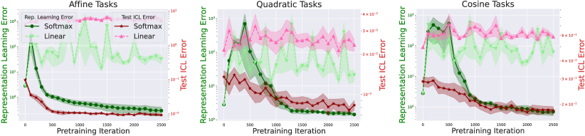
Figure 6: Representation learning error $(\rho(\mathbf{M},\mathbf{B}))$ and test ICL error (mean squared error) during pretraining softmax and linear attention on tasks from Left: $\mathcal{F}^{\text{aff}}_{\mathbf{B}}$, Center: $\mathcal{F}^{\text{2}}_{\mathbf{B}}$ , and Right: $\mathcal{F}^{\text{cos}}_{\mathbf{B}}$.

5 Conclusion

We have presented, to our knowledge, the first results showing that softmax attention learns shared structure among pretraining tasks that facilitates downstream ICL. Moreover, we have provided empirical evidence suggesting that our conclusions about what softmax attention learns during pretraining generalize to function classes beyond those considered in our analysis. Future work remains to extend our insights to multiple attention layers and general auto-regressive tasks.

Appendix A Additional Related Work

Empirical study of ICL. Several works have studied ICL of linear tasks in the framework introduced by Garg et al. (2022), and demonstrated that pretrained transformers can mimic the behavior of gradient descent (Garg et al., 2022; Akyürek et al., 2022; von Oswald et al., 2023a; Bai et al., 2023), Newton’s method (Fu et al., 2023a), and certain algorithm selection approaches (Bai et al., 2023; Li et al., 2023b). Raventós et al. (2023) studied the same linear setting with the goal of understanding the role of pretraining task diversity, while von Oswald et al. (2023b) argued via experiments on general auto-regressive tasks that ICL implicitly constructs a learning objective and optimizes it within one forward pass. Other empirical works have both directly supported (Dai et al., 2022) and contradicted (Shen et al., 2023) the hypothesis that ICL is a gradient-based optimization algorithm via experiments on real ICL tasks, while Olsson et al. (2022) empirically concluded that induction heads with softmax attention are the key mechanism that enables ICL in transformers. Lastly, outside of the context of ICL, Trockman & Kolter (2023) noticed that the attention parameter matrices of trained transformers are often close to scaled identities in practice, consistent with our findings on the importance of learning a scale to softmax attention training.

Transformer training dynamics. Huang et al. (2023) and Tian et al. (2023) studied the dynamics of softmax attention trained with gradient descent, but assumed orthonormal input features and either linear tasks (Huang et al., 2023) or that the softmax normalization is a fixed constant (Tian et al., 2023). Boix-Adsera et al. (2023) proved that softmax attention with diagonal weight matrices incrementally learns features during gradient-based training. Other work has shown that trained transformers can learn topic structure (Li et al., 2023c), spatial structure (Jelassi et al., 2022), visual features (Li et al., 2023a) and support vectors (Tarzanagh et al., 2023a, b) in specific settings disjoint from ICL.

Expressivity of transformers. Multiple works have shown that transformers with linear (von Oswald et al., 2023a, b), ReLU (Bai et al., 2023; Fu et al., 2023a; Lin et al., 2023), and softmax Akyürek et al. (2022); Giannou et al. (2023) attention are expressive enough to implement general-purpose machine learning algorithms during ICL, including gradient descent. A series of works have shown the existence of transformers that recover sparse functions of the input data (Sanford et al., 2023; Guo et al., 2023; Edelman et al., 2022; Liu et al., 2022). Fu et al. (2023b) studied the statistical complexity the learning capabilities of attention with random weights. More broadly, Pérez et al. (2021); Yun et al. (2019); Bhattamishra et al. (2020); Likhosherstov et al. (2021); Wei et al. (2022); Song et al. (2023) have analyzed various aspects of the expressivity of transformers.

Other studies of softmax attention. Wibisono & Wang (2023) hypothesized that the role of the softmax in attention is to facilitate a mixture-of-experts algorithm amenable to unstructured training data. Deng et al. (2023a) formulated a softmax regression problem and analyzed the convergence of a stylized algorithm to solve it. Han et al. (2023) showed that in a setting with ICL regression tasks a la (Garg et al., 2022), a kernel regressor akin to softmax attention with $\mathbf{M}$ equal to the inverse covariance of $\mathbf{x}$ converges to the Bayes posterior for a new ICL task – in this setting the conditional distribution of the label given the query and $n$ labelled context samples – polynomially with the number of context samples, but did not study what softmax attention learns during pretraining. Deng et al. (2023b) also compared softmax and linear attention, but focused on softmax’s greater capacity to separate data from two classes. Vuckovic et al. (2020) and Kim et al. (2020) investigate the Lipschitz constant of attention rather than what attention learns.

Appendix B Preliminaries

We first justify our claim that the first $d$ rows of the last column of $\textbf{W}_{V}$ can be set to $\mathbf{0}_{d}$ for any optimal choice of parameters.

Lemma B.1.

If under the function distribution, a function $f$ is equally likely as likely as $-f$, then any optimal solution to $\operatorname{\mathcal{L}}(\operatorname{\mathbf{W}}_{V},\operatorname{\mathbf{W}}_{K},\operatorname{\mathbf{W}}_{Q})$ in 3 satisfies $\operatorname{\mathbf{W}}_{V}=\begin{pmatrix}\mathbf{0}_{d\times d}&\mathbf{0}_{d\times 1}\\ \mathbf{0}_{1\times d}&c\end{pmatrix}$.

Proof.

For readability we write $\beta_{i}=e^{-w_{KQ}\|\operatorname{{\bf\it x}}_{i}-\operatorname{{\bf\it x}}_{n+1}\|^{2}}{\sum_{j}e^{-w_{KQ}\|\operatorname{{\bf\it x}}_{j}-\operatorname{{\bf\it x}}_{n+1}\|^{2}}}$ Suppose $\operatorname{\mathbf{W}}_{V}=\begin{pmatrix}\mathbf{0}_{d\times d}&\mathbf{v}\\ \mathbf{0}_{1\times d}&c\end{pmatrix}$ was optimal, then the loss can be written

$$\operatorname{\mathcal{L}}=\operatorname{\mathbb{E}}_{f,\{\operatorname{{\bf\it x}}_{i}\}}\left[\left(\sum_{i}c\left(f(\operatorname{{\bf\it x}}_{i})+\epsilon_{i}\right)\beta_{i}+\sum_{i}\mathbf{v}^{\top}\operatorname{{\bf\it x}}_{i}\beta_{i}-f(\operatorname{{\bf\it x}}_{n+1})\right)^{2}\right].$$

But because $f$ and $-f$ are equally likely, and because the noise is also symmetric about 0, we can write this as

$$\operatorname{\mathcal{L}} =\frac{1}{2}\operatorname{\mathbb{E}}_{f,\{\operatorname{{\bf\it x}}_{i}\},\{\epsilon_{i}\}}\left[\left(\sum_{i}c\left(f(\operatorname{{\bf\it x}}_{i})+\epsilon_{i}\right)\beta_{i}+\sum_{i}\mathbf{v}^{\top}\operatorname{{\bf\it x}}_{i}\beta_{i}-f(\operatorname{{\bf\it x}}_{n+1})\right)^{2}\right]$$

$$\quad+\frac{1}{2}\operatorname{\mathbb{E}}_{f,\{\operatorname{{\bf\it x}}_{i}\},\{\epsilon_{i}\}}\left[\left(\sum_{i}c\left((-f)(\operatorname{{\bf\it x}}_{i})-\epsilon_{i}\right)\beta_{i}+\sum_{i}\mathbf{v}^{\top}\operatorname{{\bf\it x}}_{i}\beta_{i}-(-f)(\operatorname{{\bf\it x}}_{n+1})\right)^{2}\right]$$

We can couple the noise $\{\epsilon_{i}\}$ and the data $\{\operatorname{{\bf\it x}}_{i}\}$ in the two summands above to write this as

$$\operatorname{\mathbb{E}}\left[(A+B+C)^{2}+(-A+B-C)^{2}\right],$$

where $A=\sum_{i}cf(\operatorname{{\bf\it x}}_{i})\beta_{i}-f(\operatorname{{\bf\it x}})=-\left(\sum_{i}c(-f)(\operatorname{{\bf\it x}}_{i})\beta_{i}\right)$, $B=\sum_{i}\mathbf{v}^{\top}\operatorname{{\bf\it x}}_{i}\beta_{i}$, and $C=\sum_{i}c\epsilon_{i}\beta_{i}$. We can set $B=0$ simply by setting $\mathbf{v}=\mathbf{0}_{d\times 1}$, and this has loss

$$\operatorname{\mathcal{L}} =\operatorname{\mathbb{E}}_{f,\{\operatorname{{\bf\it x}}_{i}\}}\left[\left(\sum_{i}c\left(f(\operatorname{{\bf\it x}}_{i})+\epsilon_{i}\right)\beta_{i}-f(\operatorname{{\bf\it x}}_{n+1})\right)^{2}\right]$$

$$=\frac{1}{2}\left(\operatorname{\mathbb{E}}\left[(A+C)^{2}+(-A-C)^{2}\right]\right)\leq\frac{1}{2}\left(\operatorname{\mathbb{E}}\left[(A+B+C)^{2}+(-A+B-C)^{2}\right]\right)$$

∎

In all of the distributions over functions we consider for pretraining, $f$ is equally likely as $-f$, so without loss of generality we set all elements of $\mathbf{W}_{V}$ besides the $(d+1,d+1)$-th to 0. For simplicity, we set the $(d+1,d+1)$-th element to 1.

We work with a more general data model.

Assumption B.2 (Covariate Distribution).

For each token $\operatorname{{\bf\it x}}$, first we draw $\tilde{\operatorname{{\bf\it x}}}$ as $\tilde{\operatorname{{\bf\it x}}}\sim\mathcal{U}^{d}$. Then $\operatorname{{\bf\it x}}$ is constructed as $\operatorname{{\bf\it x}}=\boldsymbol{\Sigma}^{1/2}\tilde{\operatorname{{\bf\it x}}}$.

Definition B.3 (Linear and 2-ReLU Function Classes).

The function classes $\mathcal{F}^{\text{lin}}_{L}$ and $\mathcal{F}^{+}_{L}$ are respectively defined as:

$$\mathcal{F}^{\text{lin}}_{L} :=\{f_{\mathbf{w}}:f_{\mathbf{w}}(\operatorname{{\bf\it x}})=l\mathbf{w}^{\top}\operatorname{{\bf\it x}}+b,\;\mathbf{w}\in\mathbb{S}^{d-1},\;l\in[-L,L]\},$$ (6)

$$\mathcal{F}^{+}_{L} :=\{f_{\mathbf{w}}:f_{\mathbf{w}}(\operatorname{{\bf\it x}})=l_{1}\operatorname{\text{ReLU}}(\mathbf{w}^{\top}\operatorname{{\bf\it x}})+l_{2}\operatorname{\text{ReLU}}(-\mathbf{w}^{\top}\operatorname{{\bf\it x}})+b,\;\mathbf{w}\in\mathbb{S}^{d-1}\}.$$ (7)

$D(\operatorname{\mathcal{F}}^{\text{lin}}_{L}),D(\mathcal{F}^{+}_{L})$ are induced by drawing $\mathbf{w}\sim\mathcal{N}(\mathbf{0},\boldsymbol{\Sigma}^{-1})$ and $b,l,l_{1},l_{2}\sim\text{Unif}([-L,L])$. We say that these classes are $L-$Lipschitz, because the maximum Lipschitz constant for any function in the class is $L$.

Note that because $\|\boldsymbol{\Sigma}^{-1/2}\operatorname{{\bf\it x}}_{i}\|=1$ always, we have

$$2\operatorname{{\bf\it x}}_{i}\mathbf{M}\operatorname{{\bf\it x}}_{n+1}$$

$$=\|\boldsymbol{\Sigma}^{-1/2}\operatorname{{\bf\it x}}_{i}\|^{2}+\|\boldsymbol{\Sigma}^{1/2}\mathbf{M}\boldsymbol{\Sigma}^{1/2}\boldsymbol{\Sigma}^{-1/2}\operatorname{{\bf\it x}}_{n+1}\|^{2}-\|\boldsymbol{\Sigma}^{-1/2}\operatorname{{\bf\it x}}_{i}-\boldsymbol{\Sigma}^{1/2}\mathbf{M}\boldsymbol{\Sigma}^{1/2}\boldsymbol{\Sigma}^{-1/2}\operatorname{{\bf\it x}}_{n+1}\|^{2}.$$

Let $\mathbf{M}^{\prime}=\boldsymbol{\Sigma}^{1/2}\mathbf{M}\boldsymbol{\Sigma}^{1/2}$. This means the attention estimator can be rewritten as

$$h_{SA}(\operatorname{{\bf\it x}}):=\sum_{i}\frac{f(\operatorname{{\bf\it x}}_{i})e^{\operatorname{{\bf\it x}}_{i}^{\top}\mathbf{M}\operatorname{{\bf\it x}}_{n+1}}}{\sum_{j}e^{\operatorname{{\bf\it x}}_{j}^{\top}\mathbf{M}\operatorname{{\bf\it x}}_{n+1}}}=\sum_{i}\frac{f(\operatorname{{\bf\it x}}_{i})e^{-\|\boldsymbol{\Sigma}^{-1/2}\operatorname{{\bf\it x}}_{i}-\mathbf{M}^{\prime}\boldsymbol{\Sigma}^{-1/2}\operatorname{{\bf\it x}}_{n+1}\|^{2}}}{\sum_{j}e^{-\|\boldsymbol{\Sigma}^{-1/2}\operatorname{{\bf\it x}}_{j}-\mathbf{M}^{\prime}\boldsymbol{\Sigma}^{-1/2}\operatorname{{\bf\it x}}_{n+1}\|^{2}}}$$ (8)

So the attention a token $\operatorname{{\bf\it x}}_{n+1}$ places on another $\operatorname{{\bf\it x}}_{i}$ is related to the distance between
$\mathbf{M}^{\prime}\boldsymbol{\Sigma}^{-1/2}\operatorname{{\bf\it x}}_{n+1}$ and $\boldsymbol{\Sigma}^{-1/2}\operatorname{{\bf\it x}}_{i}$. It is natural to suppose under some symmetry conditions that $\mathbf{M}^{\prime}$ is best chosen to be a scaled identity matrix so that the attention actually relates to a distance between tokens. Below we discus sufficient conditions for this.

Assumption B.4.

The function class $\operatorname{\mathcal{F}}$ and distribution $D(\mathcal{F})$ satisfy

1. $|f(\operatorname{{\bf\it x}})-f(\operatorname{{\bf\it y}})|\leq L\|\operatorname{{\bf\it x}}-\operatorname{{\bf\it y}}\|_{\boldsymbol{\Sigma}^{-1}}~{}\forall\operatorname{{\bf\it x}},\operatorname{{\bf\it y}}\in\mathcal{X}^{2},f\in\mathcal{F}$

2. $\operatorname{\mathbb{E}}_{f\sim D(\mathcal{F})}\left[f(\operatorname{{\bf\it x}})f(\operatorname{{\bf\it y}})\right]=\rho(\operatorname{{\bf\it x}}^{\top}\operatorname{{\bf\it y}})~{}\forall\operatorname{{\bf\it x}},\operatorname{{\bf\it y}}\in\mathcal{X}^{2},$ for some monotonically increasing $\rho$.

3. For any isometry $\phi$ preserving the unit sphere, and $f\in\operatorname{\mathcal{F}}$, we have $f\circ\phi\in\operatorname{\mathcal{F}}$.

Lemma B.5.

Under assumptions B.4, any minimizer of Equation ICL satisfies $\mathbf{M}^{*}=w_{KQ}\boldsymbol{\Sigma}^{-1}$ for some scalar $w_{KQ}\geq 0$.

Figure 7: Comparison between using $\mathbf{M}$ and $\omega$ in Lemma B.5. Here we denote $\operatorname{{\bf\it y}}:=\operatorname{{\bf\it y}}_{n+1}$. Under the attention induced by $\mathbf{M}$, the center of attention for $\operatorname{{\bf\it y}}$ is actually $\operatorname{{\bf\it y}}^{\prime}$, and the attention weights are depicted by the light orange shading. Under the attention induced by $\omega$, the center of attention for $\operatorname{{\bf\it y}}$ is $\operatorname{{\bf\it y}}$ and the weights are depicted by the light blue shading. Naturally, using the blue shaded attention should lead to a better estimate of $f(\mathbf{y})$ under mild regularity conditions.

Proof.

Let $\{\operatorname{{\bf\it y}}_{i}\}=\{\boldsymbol{\Sigma}^{-1/2}\operatorname{{\bf\it x}}_{i}\}$. Suppose $\mathbf{M}\operatorname{{\bf\it y}}_{n+1}\neq c\operatorname{{\bf\it y}}_{n+1}$ for any $c>0$ for some $\operatorname{{\bf\it y}}_{n+1}$. Take $c_{\operatorname{{\bf\it y}}_{n+1}}=\|\mathbf{M}\operatorname{{\bf\it y}}_{n+1}\|$ and $\operatorname{{\bf\it y}}_{n+1}^{\prime}=\frac{\mathbf{M}\operatorname{{\bf\it y}}_{n+1}}{c_{\operatorname{{\bf\it y}}_{n+1}}}$ (the projection of $\operatorname{{\bf\it y}}$ onto the sphere). Consider a function $\omega:\mathbb{R}^{d}\to\mathbb{R}^{d}$ satisfying $\omega(\operatorname{{\bf\it y}}_{n+1})=c_{\operatorname{{\bf\it y}}_{n+1}}\operatorname{{\bf\it y}}_{n+1}$. Note that this need not be linear. Let $\phi$ denote a rotation that sends $\operatorname{{\bf\it y}}^{\prime}_{n+1}$ to $\operatorname{{\bf\it y}}_{n+1}$.

We show that $\mathcal{L}(\mathbf{M})>\mathcal{L}(\omega)$, that is, it is favorable to not rotate $\operatorname{{\bf\it y}}_{n+1}$. We have

$$\operatorname{\mathcal{L}}(\mathbf{M}) =\operatorname{\mathbb{E}}_{f,\operatorname{{\bf\it y}}_{n+1},\{\operatorname{{\bf\it y}}_{i}\}}\left[\left(f(\operatorname{{\bf\it y}}_{n+1})-\frac{\sum_{i}f(\operatorname{{\bf\it y}}_{i})e^{-\|\operatorname{{\bf\it y}}_{i}-\mathbf{M}\operatorname{{\bf\it y}}_{n+1}\|^{2}}}{\sum_{j}e^{-\|\operatorname{{\bf\it y}}_{j}-\mathbf{M}\operatorname{{\bf\it y}}_{n+1}\|^{2}}}\right)^{2}\right]$$

$$=\operatorname{\mathbb{E}}_{f,\operatorname{{\bf\it y}}_{n+1},\{\operatorname{{\bf\it y}}_{i}\}}f(\operatorname{{\bf\it y}}_{n+1})^{2}+\operatorname{\mathbb{E}}_{f,\operatorname{{\bf\it y}}_{n+1},\{\operatorname{{\bf\it y}}_{i}\}}\left[\left(\frac{\sum_{i}f(\operatorname{{\bf\it y}}_{i})e^{-\|\operatorname{{\bf\it y}}_{i}-\mathbf{M}\operatorname{{\bf\it y}}_{n+1}\|^{2}}}{\sum_{j}e^{-\|\operatorname{{\bf\it y}}_{j}-\mathbf{M}\operatorname{{\bf\it y}}_{n+1}\|^{2}}}\right)^{2}\right]$$

$$\hskip 28.45274pt-2\operatorname{\mathbb{E}}_{f,\operatorname{{\bf\it y}}_{n+1},\{\operatorname{{\bf\it y}}_{i}\}}\left[\sum_{i}\frac{f(\operatorname{{\bf\it y}}_{n+1})f(\operatorname{{\bf\it y}}_{i})e^{-\|\operatorname{{\bf\it y}}_{i}-\mathbf{M}\operatorname{{\bf\it y}}_{n+1}\|^{2}}}{\sum_{j}e^{-\|\operatorname{{\bf\it y}}_{j}-\mathbf{M}\operatorname{{\bf\it y}}_{n+1}\|^{2}}}\right]$$

Lets compare this with the loss of $\omega$. For a depiction of this, please see Figure 7

$$\operatorname{\mathcal{L}}(\omega) =\operatorname{\mathbb{E}}_{f,\operatorname{{\bf\it y}}_{n+1},\{\operatorname{{\bf\it y}}_{i}\}}\left[\left(f(\operatorname{{\bf\it y}}_{n+1})-\frac{\sum_{i}f(\operatorname{{\bf\it y}}_{i})e^{-\|\operatorname{{\bf\it y}}_{i}-\omega(\operatorname{{\bf\it y}}_{n+1})\|^{2}}}{\sum_{j}e^{-\|\operatorname{{\bf\it y}}_{j}-\omega(\operatorname{{\bf\it y}}_{n+1})\|^{2}}}\right)^{2}\right]$$

$$=\operatorname{\mathbb{E}}_{f,\operatorname{{\bf\it y}}_{n+1},\{\operatorname{{\bf\it y}}_{i}\}}f(\operatorname{{\bf\it y}}_{n+1})^{2}+\operatorname{\mathbb{E}}_{f,\operatorname{{\bf\it y}}_{n+1},\{\operatorname{{\bf\it y}}_{i}\}}\left[\left(\frac{\sum_{i}f(\operatorname{{\bf\it y}}_{i})e^{-\|\operatorname{{\bf\it y}}_{i}-\omega(\operatorname{{\bf\it y}}_{n+1})\|^{2}}}{\sum_{j}e^{-\|\operatorname{{\bf\it y}}_{j}-\omega(\operatorname{{\bf\it y}}_{n+1})\|^{2}}}\right)^{2}\right]$$

$$\hskip 28.45274pt-2\operatorname{\mathbb{E}}_{f,\operatorname{{\bf\it y}}_{n+1},\{\operatorname{{\bf\it y}}_{i}\}}\left[\sum_{i}\frac{f(\operatorname{{\bf\it y}}_{n+1})f(\operatorname{{\bf\it y}}_{i})e^{-\|\operatorname{{\bf\it y}}_{i}-\omega(\operatorname{{\bf\it y}}_{n+1})\|^{2}}}{\sum_{j}e^{-\|\operatorname{{\bf\it y}}_{j}-\omega(\operatorname{{\bf\it y}}_{n+1})\|^{2}}}\right]$$

There are three terms to compare. The first in each is identical. The second is also the same:

$$\operatorname{\mathbb{E}}_{f,\operatorname{{\bf\it y}}_{n+1},\{\operatorname{{\bf\it y}}_{i}\}}\left[\left(\frac{\sum_{i}f(\operatorname{{\bf\it y}}_{i})e^{-\|\operatorname{{\bf\it y}}_{i}-\mathbf{M}\operatorname{{\bf\it y}}_{n+1}\|^{2}}}{\sum_{j}e^{-\|\operatorname{{\bf\it y}}_{j}-\mathbf{M}\operatorname{{\bf\it y}}_{n+1}\|^{2}}}\right)^{2}\right]$$

$$=\operatorname{\mathbb{E}}_{\operatorname{{\bf\it y}}_{n+1}}\operatorname{\mathbb{E}}_{f,\{\operatorname{{\bf\it y}}_{i}\}}\left[\left(\frac{\sum_{i}f(\operatorname{{\bf\it y}}_{i})e^{-\|\operatorname{{\bf\it y}}_{i}-\mathbf{M}\operatorname{{\bf\it y}}_{n+1}\|^{2}}}{\sum_{j}e^{-\|\operatorname{{\bf\it y}}_{j}-\mathbf{M}\operatorname{{\bf\it y}}_{n+1}\|^{2}}}\right)^{2}\right]$$

$$\geq\operatorname{\mathbb{E}}_{\operatorname{{\bf\it y}}_{n+1}}\operatorname{\mathbb{E}}_{f,\{\operatorname{{\bf\it y}}_{i}\}}\left[\left(\frac{\sum_{i}f(\operatorname{{\bf\it y}}_{i})e^{-\|\operatorname{{\bf\it y}}_{i}-c_{\operatorname{{\bf\it y}}_{n+1}}\operatorname{{\bf\it y}}^{\prime}\|^{2}}}{\sum_{j}e^{-\|\operatorname{{\bf\it y}}_{j}-c_{\operatorname{{\bf\it y}}_{n+1}}\operatorname{{\bf\it y}}^{\prime}\|^{2}}}\right)^{2}\right]$$

$$\geq\operatorname{\mathbb{E}}_{\operatorname{{\bf\it y}}_{n+1}}\operatorname{\mathbb{E}}_{f,\{\operatorname{{\bf\it y}}_{i}\}}\left[\left(\frac{\sum_{i}f(\phi^{-1}(\operatorname{{\bf\it y}}_{i}))e^{-\|\phi^{-1}(\operatorname{{\bf\it y}}_{i})-c_{\operatorname{{\bf\it y}}_{n+1}}\operatorname{{\bf\it y}}_{n+1}\|^{2}}}{\sum_{j}e^{-\|\phi^{-1}(\operatorname{{\bf\it y}}_{j})-c_{\operatorname{{\bf\it y}}_{n+1}}\operatorname{{\bf\it y}}_{n+1}\|^{2}}}\right)^{2}\right] \{\operatorname{{\bf\it y}}_{i}\},\operatorname{{\bf\it y}}_{n+1}$$ rotational symmetry of

$$\geq\operatorname{\mathbb{E}}_{\operatorname{{\bf\it y}}_{n+1}}\operatorname{\mathbb{E}}_{f,\{\operatorname{{\bf\it y}}_{i}\}}\left[\left(\frac{\sum_{i}f(\operatorname{{\bf\it y}}_{i})e^{-\|\operatorname{{\bf\it y}}_{i}-c_{\operatorname{{\bf\it y}}_{n+1}}\operatorname{{\bf\it y}}_{n+1}\|^{2}}}{\sum_{j}e^{-\|\operatorname{{\bf\it y}}_{j}-c_{\operatorname{{\bf\it y}}_{n+1}}\operatorname{{\bf\it y}}_{n+1}\|^{2}}}\right)^{2}\right] \{\operatorname{{\bf\it y}}_{i}\}$$ rotational symmetry of

The third takes some more work. For any choice of $\{\operatorname{{\bf\it y}}_{i}\}$, let

$$\alpha_{\operatorname{{\bf\it y}}_{n+1},\{\operatorname{{\bf\it y}}_{i}\}}(\operatorname{{\bf\it y}}_{*})=\frac{e^{-\|\operatorname{{\bf\it y}}_{n+1}-\operatorname{{\bf\it y}}_{*}\|^{2}}}{e^{-\|\operatorname{{\bf\it y}}_{n+1}-\operatorname{{\bf\it y}}_{*}\|^{2}}+\sum_{j}e^{-\|\operatorname{{\bf\it y}}_{n+1}-\operatorname{{\bf\it y}}_{i}\|^{2}}}.$$

We see that $\alpha_{\operatorname{{\bf\it y}}_{n+1},\{\operatorname{{\bf\it y}}_{i}\}}(\operatorname{{\bf\it y}}_{*})$ varies monotonically with $\operatorname{{\bf\it y}}_{n+1}^{\top}\operatorname{{\bf\it y}}_{*}$ for all $\operatorname{{\bf\it y}}_{n+1},\{\operatorname{{\bf\it y}}_{i}\}$. That is,

$$\operatorname{{\bf\it y}}_{*}^{\top}\operatorname{{\bf\it y}}_{n+1}>\operatorname{{\bf\it y}}_{*}^{\prime\top}\operatorname{{\bf\it y}}_{n+1}\implies\alpha_{\operatorname{{\bf\it y}}_{n+1},\{\operatorname{{\bf\it y}}_{i}\}}(\operatorname{{\bf\it y}}_{*})>\alpha_{\operatorname{{\bf\it y}}_{n+1},\{\operatorname{{\bf\it y}}_{i}\}}(\operatorname{{\bf\it y}}_{*}^{\prime}),$$

$$\operatorname{\mathbb{E}}_{f,\operatorname{{\bf\it y}}_{n+1},\{\operatorname{{\bf\it y}}_{i}\}}\left[\sum_{i}\frac{f(\operatorname{{\bf\it y}}_{n+1})f(\operatorname{{\bf\it y}}_{i})e^{-\|\operatorname{{\bf\it y}}_{i}-\mathbf{M}\operatorname{{\bf\it y}}_{n+1}\|^{2}}}{\sum_{j}e^{-\|\operatorname{{\bf\it y}}_{j}-\mathbf{M}\operatorname{{\bf\it y}}_{n+1}\|^{2}}}\right]$$

$$=\operatorname{\mathbb{E}}_{\operatorname{{\bf\it y}}_{n+1},\{\operatorname{{\bf\it y}}_{i}\}}\left[\sum_{i}\frac{\operatorname{\mathbb{E}}_{f}\left[f(\operatorname{{\bf\it y}}_{n+1})f(\operatorname{{\bf\it y}}_{i})\right]e^{-\|\operatorname{{\bf\it y}}_{i}-\mathbf{M}\operatorname{{\bf\it y}}_{n+1}\|^{2}}}{\sum_{j}e^{-\|\operatorname{{\bf\it y}}_{j}-\mathbf{M}\operatorname{{\bf\it y}}_{n+1}\|^{2}}}\right]$$

$$=\operatorname{\mathbb{E}}_{\operatorname{{\bf\it y}}_{n+1},\{\operatorname{{\bf\it y}}_{i}\}}\left[\sum_{i}\frac{\rho(\operatorname{{\bf\it y}}_{n+1}^{\top}\operatorname{{\bf\it y}}_{i})e^{-\|\operatorname{{\bf\it y}}_{i}-\mathbf{M}\operatorname{{\bf\it y}}_{n+1}\|^{2}}}{\sum_{j}e^{-\|\operatorname{{\bf\it y}}_{j}-\mathbf{M}\operatorname{{\bf\it y}}_{n+1}\|^{2}}}\right]$$

$$=n\operatorname{\mathbb{E}}_{\operatorname{{\bf\it y}}_{n+1},\operatorname{{\bf\it y}}_{*},\{\operatorname{{\bf\it y}}_{i}\}_{i=[n-1]}}\left[\frac{\rho(\operatorname{{\bf\it y}}_{n+1}^{\top}\operatorname{{\bf\it y}}_{*})e^{-\|\operatorname{{\bf\it y}}_{*}-\mathbf{M}\operatorname{{\bf\it y}}_{n+1}\|^{2}}}{e^{-\|\operatorname{{\bf\it y}}_{*}-\mathbf{M}\operatorname{{\bf\it y}}_{n+1}\|^{2}}+\sum_{j}e^{-\|\operatorname{{\bf\it y}}_{j}-\mathbf{M}\operatorname{{\bf\it y}}_{n+1}\|^{2}}}\right]$$

$$=n\operatorname{\mathbb{E}}_{\operatorname{{\bf\it y}}_{n+1},\operatorname{{\bf\it y}}_{*},\{\operatorname{{\bf\it y}}_{i}\}_{i=[n-1]}}\left[\rho(\operatorname{{\bf\it y}}_{n+1}^{\top}\operatorname{{\bf\it y}}_{*})\alpha_{\mathbf{M}\operatorname{{\bf\it y}}_{n+1},\{\operatorname{{\bf\it y}}_{i}\}}(\operatorname{{\bf\it y}}_{*}))\right]$$

$$=n\operatorname{\mathbb{E}}_{\operatorname{{\bf\it y}}_{n+1},\operatorname{{\bf\it y}}_{*},\{\operatorname{{\bf\it y}}_{i}\}_{i=[n-1]}}\left[\rho(\operatorname{{\bf\it y}}_{n+1}^{\top}\operatorname{{\bf\it y}}_{*})\alpha_{c_{\operatorname{{\bf\it y}}_{n+1}}\operatorname{{\bf\it y}}^{\prime},\{\operatorname{{\bf\it y}}_{i}\}}(\operatorname{{\bf\it y}}_{*}))\right]$$

$$=n\operatorname{\mathbb{E}}_{\operatorname{{\bf\it y}}_{n+1},\operatorname{{\bf\it y}}_{*},\{\operatorname{{\bf\it y}}_{i}\}_{i=[n-1]}}\left[\rho(\operatorname{{\bf\it y}}_{n+1}^{\top}\operatorname{{\bf\it y}}_{*})\alpha_{c_{\operatorname{{\bf\it y}}_{n+1}}\operatorname{{\bf\it y}}_{n+1},\{\phi^{-1}(\operatorname{{\bf\it y}}_{i})\}}(\phi^{-1}(\operatorname{{\bf\it y}}_{*})))\right]$$

$$=n\operatorname{\mathbb{E}}_{\operatorname{{\bf\it y}}_{n+1},\operatorname{{\bf\it y}}_{*},\{\operatorname{{\bf\it y}}_{i}\}_{i=[n-1]}}\left[\rho(\operatorname{{\bf\it y}}_{n+1}^{\top}\operatorname{{\bf\it y}}_{*})\alpha_{c_{\operatorname{{\bf\it y}}_{n+1}}\operatorname{{\bf\it y}}_{n+1},\{\operatorname{{\bf\it y}}_{i}\}}(\phi^{-1}(\operatorname{{\bf\it y}}_{*})))\right]$$

Similarly, we have

$$\operatorname{\mathbb{E}}_{f,\operatorname{{\bf\it y}}_{n+1},\{\operatorname{{\bf\it y}}_{i}\}}\left[\sum_{i}\frac{f(\operatorname{{\bf\it y}}_{n+1})f(\operatorname{{\bf\it y}}_{i})e^{-\|\operatorname{{\bf\it y}}_{i}-\omega(\operatorname{{\bf\it y}}_{n+1})\|^{2}}}{\sum_{j}e^{-\|\operatorname{{\bf\it y}}_{j}-\omega(\operatorname{{\bf\it y}}_{n+1})\|^{2}}}\right]$$

$$=\operatorname{\mathbb{E}}_{\operatorname{{\bf\it y}}_{n+1},\{\operatorname{{\bf\it y}}_{i}\}}\left[\sum_{i}\frac{\operatorname{\mathbb{E}}_{f}\left[f(\operatorname{{\bf\it y}}_{n+1})f(\operatorname{{\bf\it y}}_{i})\right]e^{-\|\operatorname{{\bf\it y}}_{i}-c_{\operatorname{{\bf\it y}}_{n+1}}\operatorname{{\bf\it y}}_{n+1}\|^{2}}}{\sum_{j}e^{-\|\operatorname{{\bf\it y}}_{j}-c_{\operatorname{{\bf\it y}}_{n+1}}\operatorname{{\bf\it y}}_{n+1}\|^{2}}}\right]$$

$$=\operatorname{\mathbb{E}}_{\operatorname{{\bf\it y}}_{n+1},\{\operatorname{{\bf\it y}}_{i}\}}\left[\sum_{i}\frac{\rho(\operatorname{{\bf\it y}}_{n+1}^{\top}\operatorname{{\bf\it y}}_{i})e^{-\|\operatorname{{\bf\it y}}_{i}-c_{\operatorname{{\bf\it y}}_{n+1}}\operatorname{{\bf\it y}}_{n+1}\|^{2}}}{\sum_{j}e^{-\|\operatorname{{\bf\it y}}_{j}-c_{\operatorname{{\bf\it y}}_{n+1}}\operatorname{{\bf\it y}}_{n+1}\|^{2}}}\right]$$

$$=n\operatorname{\mathbb{E}}_{\operatorname{{\bf\it y}}_{n+1},\operatorname{{\bf\it y}}_{*},\{\operatorname{{\bf\it y}}_{i}\}_{i=[n-1]}}\left[\frac{\rho(\operatorname{{\bf\it y}}_{n+1}^{\top}\operatorname{{\bf\it y}}_{*})e^{-\|\operatorname{{\bf\it y}}_{*}-c_{\operatorname{{\bf\it y}}_{n+1}}\operatorname{{\bf\it y}}_{n+1}\|^{2}}}{e^{-\|\operatorname{{\bf\it y}}_{*}-c_{\operatorname{{\bf\it y}}_{n+1}}\operatorname{{\bf\it y}}_{n+1}\|^{2}}+\sum_{j}e^{-\|\operatorname{{\bf\it y}}_{j}-c_{\operatorname{{\bf\it y}}_{n+1}}\operatorname{{\bf\it y}}_{n+1}\|^{2}}}\right]$$

$$=n\operatorname{\mathbb{E}}_{\operatorname{{\bf\it y}}_{n+1},\operatorname{{\bf\it y}}_{*},\{\operatorname{{\bf\it y}}_{i}\}_{i=[n-1]}}\left[\rho(\operatorname{{\bf\it y}}_{n+1}^{\top}\operatorname{{\bf\it y}}_{*})\alpha_{c_{\operatorname{{\bf\it y}}_{n+1}}\operatorname{{\bf\it y}}_{n+1},\{\operatorname{{\bf\it y}}_{i}\}}(\operatorname{{\bf\it y}}_{*}))\right]$$

Critically, for a given $\operatorname{{\bf\it y}}_{n+1}$, $\alpha_{\operatorname{{\bf\it y}},\{\operatorname{{\bf\it y}}_{i}\}}(\operatorname{{\bf\it y}}_{*})$ can be re-parameterized as
$\alpha_{\operatorname{{\bf\it y}}_{n+1},\{\operatorname{{\bf\it y}}_{i}\}}(\operatorname{{\bf\it y}}_{*})=\alpha^{\prime}_{\{\operatorname{{\bf\it y}}_{i}\}}(\operatorname{{\bf\it y}}_{*}-\operatorname{{\bf\it y}}_{n+1})$ where $\alpha^{\prime}_{\{\operatorname{{\bf\it y}}_{i}\}}$ is symmetric about $0$ and decreasing. Similarly, $\rho(\operatorname{{\bf\it y}}_{n+1}^{\top}\operatorname{{\bf\it y}}_{*})$ can be re-parameterized as $\rho(\operatorname{{\bf\it y}}_{n+1}^{\top}\operatorname{{\bf\it y}}_{*})=\rho^{\prime}(\operatorname{{\bf\it y}}_{*}-\operatorname{{\bf\it y}}_{n+1})$ where $\alpha^{\prime},\rho^{\prime}$ are symmetric decreasing rearrangement (that is, the set of points $\operatorname{{\bf\it z}}$ such that $\rho(\operatorname{{\bf\it x}})>r$ is a ball about the origin). From Lemma H.9 we then have

$$\operatorname{\mathbb{E}}_{\operatorname{{\bf\it y}}_{n+1}}\operatorname{\mathbb{E}}{\operatorname{{\bf\it y}}_{*},\{\operatorname{{\bf\it y}}_{i}\}_{i=[n-1]}}\left[\rho(\operatorname{{\bf\it y}}_{n+1}^{\top}\operatorname{{\bf\it y}}_{*})\alpha_{c_{\operatorname{{\bf\it y}}_{n+1}}\operatorname{{\bf\it y}}_{n+1},\{\operatorname{{\bf\it y}}_{i}\}}(\phi^{-1}(\operatorname{{\bf\it y}}_{*}))\right]$$

$$\hskip 5.69046pt=\operatorname{\mathbb{E}}_{\operatorname{{\bf\it y}}_{n+1}}\operatorname{\mathbb{E}}{\operatorname{{\bf\it y}}_{*},\{\operatorname{{\bf\it y}}_{i}\}_{i=[n-1]}}\left[\rho^{\prime}(\|\operatorname{{\bf\it y}}_{n+1}-\operatorname{{\bf\it y}}_{*}\|)\alpha_{\{\operatorname{{\bf\it y}}_{i}\}}(\|\operatorname{{\bf\it y}}_{n+1}-\phi^{-1}\operatorname{{\bf\it y}}_{*}\|)\right]$$

$$\hskip 5.69046pt<\operatorname{\mathbb{E}}_{\operatorname{{\bf\it y}}_{n+1}}\operatorname{\mathbb{E}}{\operatorname{{\bf\it y}}_{*},\{\operatorname{{\bf\it y}}_{i}\}_{i=[n-1]}}\left[\rho^{\prime}(\|\operatorname{{\bf\it y}}_{n+1}-\operatorname{{\bf\it y}}_{*}\|)\alpha_{\{\operatorname{{\bf\it y}}_{i}\}}(\|\operatorname{{\bf\it y}}_{n+1}-\operatorname{{\bf\it y}}_{*}\|)\right]$$

$$\hskip 5.69046pt=\operatorname{\mathbb{E}}_{\operatorname{{\bf\it y}}_{n+1}}\operatorname{\mathbb{E}}{\operatorname{{\bf\it y}}_{*},\{\operatorname{{\bf\it y}}_{i}\}_{i=[n-1]}}\left[\rho(\operatorname{{\bf\it y}}_{n+1}^{\top}\operatorname{{\bf\it y}}_{*})\alpha_{c_{\operatorname{{\bf\it y}}_{n+1}}\operatorname{{\bf\it y}}_{n+1},\{\operatorname{{\bf\it y}}_{i}\}}(\operatorname{{\bf\it y}}_{*})\right]$$

So $\operatorname{\mathcal{L}}(\omega)<\operatorname{\mathcal{L}}(\mathbf{M})$. Let

$$q(c_{\operatorname{{\bf\it y}}_{n+1}})=\operatorname{\mathbb{E}}_{f,\{\operatorname{{\bf\it y}}_{i}\}}\left[\left(f(\operatorname{{\bf\it y}}_{n+1})-\frac{\sum_{i}f(\operatorname{{\bf\it y}}_{i})e^{-\|\operatorname{{\bf\it y}}_{i}-c_{\operatorname{{\bf\it y}}_{n+1}}\operatorname{{\bf\it y}}_{n+1}\|^{2}}}{\sum_{j}e^{-\|\operatorname{{\bf\it y}}_{j}-c_{\operatorname{{\bf\it y}}_{n+1}}\operatorname{{\bf\it y}}_{n+1}\|^{2}}}\right)^{2}\right].$$

Observe that $\operatorname{\mathcal{L}}(\omega)=\operatorname{\mathbb{E}}_{\operatorname{{\bf\it y}}_{n+1}}q(c_{\operatorname{{\bf\it y}}_{n+1}})$. We might as well set $\omega$ to be such that $c_{\operatorname{{\bf\it y}}_{n+1}}$ is the same for all $\operatorname{{\bf\it y}}_{n+1}$ and a minimizer of $q$, so we have $\omega(\operatorname{{\bf\it y}}_{n+1})=c\operatorname{{\bf\it y}}_{n+1}$ for all $\operatorname{{\bf\it y}}_{n+1}$ which implies $\omega=c\mathbf{I}_{d}$ for some $c$. Because the optimal $\mathbf{M}^{\prime}$ is identity, the corresponding optimal $\mathbf{M}$ is $\boldsymbol{\Sigma}^{-1}$. ∎

B.1 Rewriting the Loss

As a result of this, we can take $\mathbf{M}=w_{KQ}\boldsymbol{\Sigma}^{-1}$ and write the attention estimator as

$$h_{SA}(\operatorname{{\bf\it x}})=\sum_{i}\frac{f(\operatorname{{\bf\it x}}_{i})e^{-w_{KQ}\|\boldsymbol{\Sigma}^{-1/2}\operatorname{{\bf\it x}}_{i}-\boldsymbol{\Sigma}^{-1/2}\operatorname{{\bf\it x}}_{n+1}\|^{2}}}{\sum_{j}e^{-w_{KQ}\|\boldsymbol{\Sigma}^{-1/2}\operatorname{{\bf\it x}}_{j}-\boldsymbol{\Sigma}^{-1/2}\operatorname{{\bf\it x}}_{n+1}\|^{2}}}$$ (9)

This allows us to make the transformation $\operatorname{\mathcal{X}}\to\boldsymbol{\Sigma}^{-1/2}\operatorname{\mathcal{X}}$. This has the effect of making both the data covariance and the induced function class covariance equal to the identity. Essentially, WLOG we will henceforth consider $\boldsymbol{\Sigma}=\mathbf{I}_{d}$. Henceforth, the estimator will be taken to be

$$h_{SA}(\operatorname{{\bf\it x}})=\sum_{i}\frac{f(\operatorname{{\bf\it x}}_{i})e^{-w_{KQ}\|\operatorname{{\bf\it x}}_{i}-\operatorname{{\bf\it x}}_{n+1}\|^{2}}}{\sum_{j}e^{-w_{KQ}\|\operatorname{{\bf\it x}}_{j}-\operatorname{{\bf\it x}}_{n+1}\|^{2}}}$$ (10)

and the loss will be parameterized by $w_{KQ}$ as

$$\operatorname{\mathcal{L}}(w_{KQ})=\operatorname{\mathbb{E}}_{f,\{\operatorname{{\bf\it x}}_{i}\}}\left[\left(\sum_{i}\frac{\left(f(\operatorname{{\bf\it x}}_{i})+\epsilon_{i}\right)e^{-w_{KQ}\|\operatorname{{\bf\it x}}_{i}-\operatorname{{\bf\it x}}_{n+1}\|^{2}}}{\sum_{j}e^{-w_{KQ}\|\operatorname{{\bf\it x}}_{j}-\operatorname{{\bf\it x}}_{n+1}\|^{2}}}-f(\operatorname{{\bf\it x}}_{n+1})\right)^{2}\right].$$

Because the noise $\epsilon_{i}$ is independent of everything else, we can decompose this into two terms, a signal term and a noise term as follows

$$\operatorname{\mathcal{L}}(w_{KQ}) =\underbrace{\operatorname{\mathbb{E}}_{f,\{\operatorname{{\bf\it x}}_{i}\}}\left[\left(\sum_{i}\frac{\left(f(\operatorname{{\bf\it x}}_{n+1})-f(\operatorname{{\bf\it x}}_{i})\right)e^{-w_{KQ}\|\operatorname{{\bf\it x}}_{i}-\operatorname{{\bf\it x}}_{n+1}\|^{2}}}{\sum_{j}e^{-w_{KQ}\|\operatorname{{\bf\it x}}_{j}-\operatorname{{\bf\it x}}_{n+1}\|^{2}}}\right)^{2}\right]}_{\operatorname{\mathcal{L}_{\text{signal}}}(w_{KQ})}$$

$$\hskip 28.45274pt+\underbrace{\operatorname{\mathbb{E}}_{f,\{\operatorname{{\bf\it x}}_{i}\}}\left[\left(\sum_{i}\frac{\epsilon_{i}e^{-w_{KQ}\|\operatorname{{\bf\it x}}_{i}-\operatorname{{\bf\it x}}_{n+1}\|^{2}}}{\sum_{j}e^{-w_{KQ}\|\operatorname{{\bf\it x}}_{j}-\operatorname{{\bf\it x}}_{n+1}\|^{2}}}-f(\operatorname{{\bf\it x}}_{n+1})\right)^{2}\right]}_{\operatorname{\mathcal{L}_{\text{noise}}}(w_{KQ})}$$

We bound the first term in Appendix C and the second in Appendix D. A useful function that we bound in Lemma H.4 and Corrolary H.5 in Appendix H is

$$g_{p}(r)=\sum_{i=1}^{n}\|\operatorname{{\bf\it x}}_{i}-\operatorname{{\bf\it x}}\|^{p}e^{-r\|\operatorname{{\bf\it x}}_{i}^{\top}-\operatorname{{\bf\it x}}^{2}\|}.$$

We will use this function, particularly for $p=0$ and $1$.

Appendix C The Signal Term

The purpose of this section of the Appendix is to obtain upper and lower bounds on $\operatorname{\mathcal{L}_{\text{signal}}}(w_{KQ})$. Because we work with two different distributions over functions, and because the bounds depend on the distributions, we will make the distribution explicit in the argument to the function

$$\operatorname{\mathcal{L}_{\text{signal}}}(w_{KQ};D(\operatorname{\mathcal{F}}))=\operatorname{\mathbb{E}}_{f,\{\operatorname{{\bf\it x}}\}}\left(f(\operatorname{{\bf\it x}}_{i})-\sum_{i}\frac{f(\operatorname{{\bf\it x}}_{i})e^{-w_{KQ}\|\operatorname{{\bf\it x}}_{i}-\operatorname{{\bf\it x}}_{n+1}\|^{2}}}{\sum_{j}e^{-w_{KQ}\|\operatorname{{\bf\it x}}_{j}-\operatorname{{\bf\it x}}_{n+1}\|^{2}}}\right)^{2}$$

As a reminder, we consider the following two distributions over functions

Definition C.1 (Linear and 2-ReLU Function Classes).

The function classes $\mathcal{F}_{\text{linear}}$ and $\mathcal{F}_{\text{nonlinear}}$ are respectively defined as:

$$\mathcal{F}_{L} :=\{f:f(\operatorname{{\bf\it x}})=l\mathbf{w}^{\top}\operatorname{{\bf\it x}}+b,\;\mathbf{w}\in\mathbb{S}^{d-1}\},$$

$$\mathcal{F}_{L}^{+} :=\{f:f(\operatorname{{\bf\it x}})=l_{1}\operatorname{\text{ReLU}}(\mathbf{w}^{\top}\operatorname{{\bf\it x}})+l_{2}\operatorname{\text{ReLU}}(-\mathbf{w}^{\top}\operatorname{{\bf\it x}})+b,\;\mathbf{w}\in\mathbb{S}^{d-1}\}.$$

$D(\operatorname{\mathcal{F}}_{L}),D(\operatorname{\mathcal{F}}_{L}^{+})$ are induced by taking $\mathbf{w}\sim\mathcal{N}(\mathbf{0}_{d\times d},\mathbf{I}_{d})$, $b,l,l_{1},l_{2}\sim\text{Unif}[-L,L]$.

First we have the following trivial bound on $\operatorname{\mathcal{L}_{\text{signal}}}(w_{KQ})$.

Lemma C.2.

For all $w_{KQ}$ we have $\operatorname{\mathcal{L}_{\text{signal}}}(w_{KQ})\leq 4L^{2}$.

Proof.

We have $\operatorname{\mathcal{L}_{\text{signal}}}(w_{KQ})\leq\operatorname{\mathbb{E}}\left[\left(\sum\frac{f(\operatorname{{\bf\it x}}_{i})-f(\operatorname{{\bf\it x}}_{n+1})\gamma_{i}}{\sum\gamma_{i}}\right)^{2}\right]$ for some positive $\{\gamma_{i}\}$. By Lipschitzness, $f(\operatorname{{\bf\it x}}_{i})-f(\operatorname{{\bf\it x}}_{n+1})\leq L\|\operatorname{{\bf\it x}}_{i}-\operatorname{{\bf\it x}}_{n+1}\|\leq 2L$. ∎

C.1 Linear functions

Here we consider the linear function class $\operatorname{\mathcal{F}}_{L}$. First, we note that this class satisfies Assumption B.4.

Lemma C.3.

The linear class $\operatorname{\mathcal{F}}_{L}$ in Definition 3.2 satisfies Assumption B.4.

Proof.

1. We have $|f(\operatorname{{\bf\it x}})-f(\operatorname{{\bf\it y}})|=|\mathbf{w}^{\top}(\operatorname{{\bf\it x}}-\operatorname{{\bf\it y}})|\leq\|\mathbf{w}\|\|\operatorname{{\bf\it x}}-\operatorname{{\bf\it y}}\|$ by Cauchy-Schwarz.

2. Because $b$ is independent of $w$, we have

   $$\operatorname{\mathbb{E}}_{f}\left[f(\operatorname{{\bf\it x}})f(\operatorname{{\bf\it y}})\right]=\operatorname{\mathbb{E}}_{\mathbf{w}}\left[l^{2}\operatorname{{\bf\it x}}^{\top}\mathbf{ww}^{\top}\operatorname{{\bf\it y}}+b^{2}\right]=\operatorname{\mathbb{E}}l^{2}\frac{\operatorname{\mathbb{E}}_{\mathbf{w}}\|\mathbf{w}\|^{2}}{d}\operatorname{{\bf\it x}}^{\top}\operatorname{{\bf\it y}}+\frac{L^{2}}{3}.$$

3. $\mathbf{w}$ is isotropic, so $\phi(\mathbf{w})$ is also supported by the distribution on $\mathbf{w}$.

∎

Lemma C.4.

For linear functions, the signal term is upper bounded as

$$\operatorname{\mathcal{L}_{\text{signal}}}(w_{KQ};D(\operatorname{\mathcal{F}}_{L}))\leq\begin{cases}L^{2}\operatorname{\mathcal{O}}\left(\frac{1}{w^{2}_{KQ}}+\frac{w_{KQ}^{\frac{d}{2}-1}}{n}+\frac{1}{n}\right)&w_{KQ}\geq\frac{d+\sqrt{d}}{2}\\ 4L^{2}&w_{KQ}<\frac{d+\sqrt{d}}{2}\end{cases}$$

Proof.

In the interest of readability, we will denote $\operatorname{{\bf\it x}}_{n+1}$ as $\operatorname{{\bf\it x}}$. Consider $\tilde{\operatorname{{\bf\it x}}}$ such that  $\tilde{\operatorname{{\bf\it x}}}=\sum_{i}\operatorname{{\bf\it x}}_{i}\frac{e^{-2w_{KQ}\operatorname{{\bf\it x}}_{i}^{\top}\operatorname{{\bf\it x}}}}{\sum_{j}e^{-2w_{KQ}\operatorname{{\bf\it x}}_{i}^{\top}\operatorname{{\bf\it x}}}}$. Then our loss is given by $\operatorname{\mathbb{E}}\left[l^{2}\mathbf{w}^{\top}(\operatorname{{\bf\it x}}-\tilde{\operatorname{{\bf\it x}}})\right]^{2}$. First, since $\mathbf{w}$ is independent of $\operatorname{{\bf\it x}},\{\operatorname{{\bf\it x}}_{i}\}$, we have $\operatorname{\mathbb{E}}l^{2}\left(\mathbf{w}^{\top}(\operatorname{{\bf\it x}}-\tilde{\operatorname{{\bf\it x}}})\right)^{2}=\operatorname{\mathbb{E}}l^{2}\mathbf{ww}^{\top}(\operatorname{{\bf\it x}}-\tilde{\operatorname{{\bf\it x}}})(\operatorname{{\bf\it x}}-\tilde{\operatorname{{\bf\it x}}})^{\top}$, Now $\mathbf{w}$ has a uniformly randomly chosen direction, so its covariance is a multiple of the identity. We have $\operatorname{\mathbb{E}}\text{Tr}(\mathbf{ww}^{\top})=\operatorname{\mathbb{E}}\|\mathbf{w}\|^{2}=\frac{L^{2}}{3}$, so $\operatorname{\mathbb{E}}l^{2}\mathbf{ww}^{\top}=\frac{L^{2}}{3d}\mathbf{I}_{d}$. Continuing, $\operatorname{\mathbb{E}}\left(\mathbf{w}^{\top}(\operatorname{{\bf\it x}}-\tilde{\operatorname{{\bf\it x}}})\right)^{2}=\frac{L^{2}}{3d}\operatorname{\mathbb{E}}\|\operatorname{{\bf\it x}}-\tilde{\operatorname{{\bf\it x}}}\|^{2}$. Take any $\operatorname{{\bf\it x}}^{\prime}\perp\operatorname{{\bf\it x}}$, we have

$$\operatorname{\mathbb{E}}\tilde{\operatorname{{\bf\it x}}}^{\top}\operatorname{{\bf\it x}}^{\prime} =\operatorname{\mathbb{E}}\sum_{i}\operatorname{{\bf\it x}}_{i}^{\top}\operatorname{{\bf\it x}}^{\prime}\frac{e^{-2w_{KQ}\operatorname{{\bf\it x}}_{i}^{\top}\operatorname{{\bf\it x}}}}{\sum_{j}e^{-2w_{KQ}\operatorname{{\bf\it x}}_{i}^{\top}\operatorname{{\bf\it x}}}}$$

$$=\operatorname{\mathbb{E}}\sum_{i}\operatorname{\mathbb{E}}[\operatorname{{\bf\it x}}_{i}^{\top}\operatorname{{\bf\it x}}^{\prime}\mid\operatorname{{\bf\it x}}_{i}^{\top}]\frac{e^{-2w_{KQ}\operatorname{{\bf\it x}}_{i}^{\top}\operatorname{{\bf\it x}}}}{\sum_{j}e^{-2w_{KQ}\operatorname{{\bf\it x}}_{i}^{\top}\operatorname{{\bf\it x}}}}=0$$ iterated expectation and symmetry

Decomposing $\tilde{\operatorname{{\bf\it x}}}$ into an orthogonal and a parallel component, we have $\operatorname{\mathbb{E}}\|\operatorname{{\bf\it x}}-\tilde{\operatorname{{\bf\it x}}}\|^{2}=\operatorname{\mathbb{E}}\|\operatorname{{\bf\it x}}-\operatorname{{\bf\it x}}\operatorname{{\bf\it x}}^{\top}\tilde{\operatorname{{\bf\it x}}}-\operatorname{{\bf\it x}}^{\prime}\operatorname{{\bf\it x}}^{\prime\top}\tilde{\operatorname{{\bf\it x}}}\|^{2}$ for some $\operatorname{{\bf\it x}}^{\prime}\perp\operatorname{{\bf\it x}}$ with $\|\operatorname{{\bf\it x}}^{\prime}\|=1$. But

$$\operatorname{\mathbb{E}}\|\operatorname{{\bf\it x}}-\operatorname{{\bf\it x}}\operatorname{{\bf\it x}}^{\top}\tilde{\operatorname{{\bf\it x}}}-\operatorname{{\bf\it x}}^{\prime}\operatorname{{\bf\it x}}^{\prime\top}\tilde{\operatorname{{\bf\it x}}}\|^{2}$$

$$=\operatorname{\mathbb{E}}\|\operatorname{{\bf\it x}}(1-\operatorname{{\bf\it x}}^{\top}\tilde{\operatorname{{\bf\it x}}})\|^{2}+\operatorname{\mathbb{E}}\|\operatorname{{\bf\it x}}^{\prime}\operatorname{{\bf\it x}}^{\prime\top}\tilde{\operatorname{{\bf\it x}}}\|^{2}-2\operatorname{\mathbb{E}}\operatorname{{\bf\it x}}(1-\operatorname{{\bf\it x}}^{\top}\tilde{\operatorname{{\bf\it x}}})\tilde{\operatorname{{\bf\it x}}}^{\top}\operatorname{{\bf\it x}}^{\prime}\operatorname{{\bf\it x}}^{\prime\top}$$

$$=\operatorname{\mathbb{E}}\|\operatorname{{\bf\it x}}(1-\operatorname{{\bf\it x}}^{\top}\tilde{\operatorname{{\bf\it x}}})\|^{2}+\operatorname{\mathbb{E}}\|\operatorname{{\bf\it x}}^{\prime}\operatorname{{\bf\it x}}^{\prime\top}\tilde{\operatorname{{\bf\it x}}}\|^{2}\hskip 28.45274pt\because\operatorname{{\bf\it x}}^{\top}\operatorname{{\bf\it x}}^{\prime}=0\implies 2\operatorname{\mathbb{E}}\operatorname{{\bf\it x}}(1-\operatorname{{\bf\it x}}^{\top}\tilde{\operatorname{{\bf\it x}}})\tilde{\operatorname{{\bf\it x}}}^{\top}\operatorname{{\bf\it x}}^{\prime}\operatorname{{\bf\it x}}^{\prime\top}=0$$ (11)

Case 1: $w_{KQ}\geq\frac{d+\sqrt{d}}{2}$.

Consider first the term $\operatorname{\mathbb{E}}\|\operatorname{{\bf\it x}}(1-\operatorname{{\bf\it x}}^{\top}\tilde{\operatorname{{\bf\it x}}})\|^{2}=\operatorname{\mathbb{E}}(1-\operatorname{{\bf\it x}}^{\top}\tilde{\operatorname{{\bf\it x}}})^{2}$. Here we have with probability $1-\frac{1}{n}$

$$1-\operatorname{{\bf\it x}}^{\top}\tilde{\operatorname{{\bf\it x}}}=\frac{\sum(1-\operatorname{{\bf\it x}}^{\top}\operatorname{{\bf\it x}}_{i})e^{-w_{KQ}\|\operatorname{{\bf\it x}}-\operatorname{{\bf\it x}}_{i}\|^{2}}}{\sum e^{-w_{KQ}\|\operatorname{{\bf\it x}}-\operatorname{{\bf\it x}}_{i}\|^{2}}}=\frac{g_{2}(w_{KQ})}{2g_{0}(w_{KQ})}$$

$$\leq\frac{\overline{C_{b}}n\left(\frac{1}{w_{KQ}}\right)^{\frac{d}{2}+1}}{2\underline{C_{b}}n\left(\frac{1}{w_{KQ}}\right)^{\frac{d}{2}}}\leq\frac{\overline{C_{b}}}{\underline{C_{b}}}\frac{1}{w_{KQ}}$$ Corollary H.5 (12)

The other term $\operatorname{\mathbb{E}}\|\operatorname{{\bf\it x}}^{\prime}\operatorname{{\bf\it x}}^{\prime\top}\tilde{\operatorname{{\bf\it x}}}\|^{2}=\operatorname{\mathbb{E}}(\operatorname{{\bf\it x}}^{\prime\top}\tilde{\operatorname{{\bf\it x}}})^{2}$ is the component of the bias in the direction orthogonal to $\operatorname{{\bf\it x}}$.

$$(\operatorname{{\bf\it x}}^{\prime\top}\tilde{\operatorname{{\bf\it x}}})^{2}=\left(\frac{\sum_{i}\operatorname{{\bf\it x}}^{\prime\top}\operatorname{{\bf\it x}}_{i}e^{-w_{KQ}\|\operatorname{{\bf\it x}}_{i}-\operatorname{{\bf\it x}}\|^{2}}}{\sum_{i}e^{-w_{KQ}\|\operatorname{{\bf\it x}}_{i}-\operatorname{{\bf\it x}}\|^{2}}}\right)^{2}$$

$$\quad\leq\left(\frac{\sum_{i}\operatorname{{\bf\it x}}^{\prime\top}\operatorname{{\bf\it x}}_{i}e^{-w_{KQ}\|\operatorname{{\bf\it x}}_{i}-\operatorname{{\bf\it x}}\|^{2}}}{\sum_{i}e^{-w_{KQ}\|\operatorname{{\bf\it x}}_{i}-\operatorname{{\bf\it x}}\|^{2}}}\right)^{2}$$

$$\quad\leq\left(\frac{\sum_{i}\operatorname{{\bf\it x}}^{\prime\top}\operatorname{{\bf\it x}}_{i}e^{-w_{KQ}\|\operatorname{{\bf\it x}}_{i}-\operatorname{{\bf\it x}}\|^{2}}}{\sum_{i}e^{-w_{KQ}\|\operatorname{{\bf\it x}}_{i}-\operatorname{{\bf\it x}}\|^{2}}}\right)^{2}$$

$$\quad\leq\frac{\sum_{i}\left(1-(\operatorname{{\bf\it x}}^{\top}\operatorname{{\bf\it x}}_{i})^{2}\right)e^{-2w_{KQ}\|\operatorname{{\bf\it x}}_{i}-\operatorname{{\bf\it x}}\|^{2}}}{\left(\sum_{i}e^{-w_{KQ}\|\operatorname{{\bf\it x}}_{i}-\operatorname{{\bf\it x}}_{n}\|^{2}}\right)^{2}}$$ Popoviciu’s Variance inequality

$$\quad\leq\frac{\sum_{i}2\left(1-\operatorname{{\bf\it x}}^{\top}\operatorname{{\bf\it x}}_{i}\right)e^{-2w_{KQ}\|\operatorname{{\bf\it x}}_{i}-\operatorname{{\bf\it x}}\|^{2}}}{\left(\sum_{i}e^{-w_{KQ}\|\operatorname{{\bf\it x}}_{i}-\operatorname{{\bf\it x}}\|^{2}}\right)^{2}}$$

$$\quad\leq\frac{\sum_{i}\|\operatorname{{\bf\it x}}_{i}-\operatorname{{\bf\it x}}\|^{2}e^{-2w_{KQ}\|\operatorname{{\bf\it x}}_{i}-\operatorname{{\bf\it x}}\|^{2}}}{\left(\sum_{i}e^{-w_{KQ}\|\operatorname{{\bf\it x}}_{i}-\operatorname{{\bf\it x}}\|^{2}}\right)^{2}}=\frac{g_{2}(2w_{KQ})}{g_{0}^{2}(w_{KQ})}$$

With probability $1-\frac{1}{n}$, when $w_{KQ}\geq d+\sqrt{d}$ we have

$$\frac{g_{2}(2w_{KQ})}{g_{0}(w_{KQ})^{2}} \leq\frac{\overline{c_{g}}n\left(\frac{1}{2w_{KQ}}\right)^{\frac{d}{2}+1}}{\left(\underline{c_{g}}n\left(\frac{1}{w_{KQ}}\right)^{\frac{d}{2}}\right)^{2}}\leq\frac{\overline{c_{g}}w_{KQ}^{\frac{d}{2}-1}}{\underline{c_{g}}^{2}2^{\frac{d}{2}+1}n}$$ (13)

Putting together Equations 12 and 13, we have with probability $1-\frac{1}{n}$,

$$\operatorname{\mathcal{L}_{\text{signal}}}(w_{KQ};D(\operatorname{\mathcal{F}}_{L}))\leq\operatorname{\mathcal{O}}\left(\frac{L^{2}}{3d}\left(\frac{1}{w_{KQ}}+\frac{w_{KQ}^{\frac{d}{2}-1}}{n}\right)\right).$$

The signal bias is upper bounded by $4L^{2}$ always (Lemma C.2). The overall upper-bound on the expectation is

$$\operatorname{\mathcal{L}_{\text{signal}}}(w_{KQ};D(\operatorname{\mathcal{F}}_{L}))\leq\operatorname{\mathcal{O}}\left(\frac{L^{2}}{3d}\left(\frac{1}{w_{KQ}}+\frac{w_{KQ}^{\frac{d}{2}-1}}{n}+4\right)\right).$$

Case 2: $w_{KQ}<\frac{d+\sqrt{d}}{2}$. We always have $\operatorname{\mathcal{L}}(w_{KQ})\leq 4L^{2}$ from Lemma C.2. ∎

Lemma C.5.

For linear functions, the signal term is lower bounded as

$$\operatorname{\mathcal{L}_{\text{signal}}}(w_{KQ};D(\operatorname{\mathcal{F}}_{L}))\geq\begin{cases}\Omega\left(\frac{L^{2}}{w^{2}_{KQ}}\right)&w_{KQ}>\frac{d+\sqrt{d}}{2}\\ \Omega\left(1\right)&w_{KQ}<\frac{d+\sqrt{d}}{2}\end{cases}.$$

Proof.

Similar to Equation (11), for $\tilde{\operatorname{{\bf\it x}}}=\sum_{i}\operatorname{{\bf\it x}}_{i}\frac{e^{-2w_{KQ}\operatorname{{\bf\it x}}_{i}^{\top}\operatorname{{\bf\it x}}}}{\sum_{j}e^{-2w_{KQ}\operatorname{{\bf\it x}}_{i}^{\top}\operatorname{{\bf\it x}}}}$, we have

$$\operatorname{\mathcal{L}_{\text{signal}}}(w_{KQ};D(\operatorname{\mathcal{F}}_{L}))\geq\frac{L^{2}}{3d}\operatorname{\mathbb{E}}\|\operatorname{{\bf\it x}}(1-\operatorname{{\bf\it x}}^{\top}\tilde{\operatorname{{\bf\it x}}})\|^{2}=\frac{L^{2}}{3d}\operatorname{\mathbb{E}}(1-\operatorname{{\bf\it x}}^{\top}\tilde{\operatorname{{\bf\it x}}})^{2}$$

Now consider the term $1-\operatorname{{\bf\it x}}^{\top}\tilde{\operatorname{{\bf\it x}}}$. We have

$$\frac{\sum(1-\operatorname{{\bf\it x}}^{\top}\operatorname{{\bf\it x}}_{i})e^{-w_{KQ}\|\operatorname{{\bf\it x}}-\operatorname{{\bf\it x}}_{i}\|^{2}}}{\sum e^{-w_{KQ}\|\operatorname{{\bf\it x}}-\operatorname{{\bf\it x}}_{i}\|^{2}}}\geq\frac{g_{2}(w_{KQ})}{2g_{0}(w_{KQ})}$$

Case 1: $w_{KQ}\geq\frac{d+\sqrt{d}}{2}$. Here we have from Corollary H.5, with probability $1-1/n$

$$\frac{\sum(1-\operatorname{{\bf\it x}}^{\top}\operatorname{{\bf\it x}}_{i})e^{-w_{KQ}\|\operatorname{{\bf\it x}}-\operatorname{{\bf\it x}}_{i}\|^{2}}}{\sum e^{-w_{KQ}\|\operatorname{{\bf\it x}}-\operatorname{{\bf\it x}}_{i}\|^{2}}}\geq\frac{\underline{C_{b}}n\left(\frac{1}{w_{KQ}}\right)^{\frac{d}{2}+1}}{2\overline{C_{b}}n\left(\frac{1}{w_{KQ}}\right)^{\frac{d}{2}}}\geq\frac{\underline{C_{b}}}{2\overline{C_{b}}}\frac{1}{w_{KQ}}.$$

With probability $1/n\leq\frac{1}{2}$ the lowest we can have is $\operatorname{\mathcal{L}_{\text{signal}}}(w_{KQ})=0$, so overall we have

$$\operatorname{\mathcal{L}_{\text{signal}}}(w_{KQ})\geq\frac{L^{2}}{24d}\left(\frac{\underline{C_{b}}}{\overline{C_{b}}}\frac{1}{w_{KQ}}\right)^{2}$$

Case 2: $\frac{d+\sqrt{d}}{4}\leq w_{KQ}\leq\frac{d+\sqrt{d}}{2}$. From Corollary H.5, with probability $1-\frac{1}{n}$

$$\frac{\sum(1-\operatorname{{\bf\it x}}^{\top}\operatorname{{\bf\it x}}_{i})e^{-w_{KQ}\|\operatorname{{\bf\it x}}-\operatorname{{\bf\it x}}_{i}\|^{2}}}{\sum e^{-w_{KQ}\|\operatorname{{\bf\it x}}-\operatorname{{\bf\it x}}_{i}\|^{2}}}\geq\frac{\underline{C_{b}}n\left(\frac{1}{w_{KQ}}\right)^{\frac{d}{2}+1}}{2\overline{C_{b}}ne^{-2w_{KQ}}}\geq\frac{\underline{C_{b}}}{2\overline{C_{b}}}\frac{e^{2w_{KQ}}}{w_{KQ}^{\frac{d}{2}+1}}.$$

With probability $1/n\leq\frac{1}{2}$ the lowest we can have is $\operatorname{\mathcal{L}_{\text{signal}}}(w_{KQ})=0$, so overall we have

$$\operatorname{\mathcal{L}_{\text{signal}}}(w_{KQ})\geq\frac{L^{2}}{24d}\left(\frac{\underline{C_{b}}}{\overline{C_{b}}}\frac{e^{2w_{KQ}}}{w_{KQ}^{\frac{d}{2}+1}}\right)^{2}$$

Case 3: $\frac{d+\sqrt{d}}{4}>w_{KQ}$. From Corollary H.5, with probability $1-\frac{1}{n}$

$$\frac{\sum(1-\operatorname{{\bf\it x}}^{\top}\operatorname{{\bf\it x}}_{i})e^{-w_{KQ}\|\operatorname{{\bf\it x}}-\operatorname{{\bf\it x}}_{i}\|^{2}}}{\sum e^{-w_{KQ}\|\operatorname{{\bf\it x}}-\operatorname{{\bf\it x}}_{i}\|^{2}}}\geq\frac{\underline{C_{b}}ne^{-4w_{KQ}}}{2\overline{C_{b}}ne^{-2w_{KQ}}}\geq\frac{\underline{C_{b}}}{2\overline{C_{b}}}e^{-2w_{KQ}}.$$

With probability $1/n\leq\frac{1}{2}$ the lowest we can have is $\operatorname{\mathcal{L}_{\text{signal}}}(w_{KQ})=0$, so overall we have

$$\operatorname{\mathcal{L}_{\text{signal}}}(w_{KQ})\geq\frac{L^{2}}{24d}\left(\frac{\underline{C_{b}}}{\overline{C_{b}}}e^{-2w_{KQ}}\right)^{2}$$

∎

Corollary C.6.

Combining the above, we have

$$L^{2}\operatorname{\mathcal{O}}\left(\frac{1}{\left(w_{KQ}+1\right)^{2}}\right)\leq\operatorname{\mathcal{L}_{\text{signal}}}(w_{KQ};D(\operatorname{\mathcal{F}}_{L}))\leq L^{2}\operatorname{\mathcal{O}}\left(\frac{1}{w_{KQ}^{2}}+\frac{w_{KQ}^{\frac{d}{2}-1}}{n}+\frac{1}{n}\right).$$ (14)

We can now perturb these bounds in the case of a nonlinear function class.

C.2 Nonlinear functions

Consider the function class

$$\mathcal{F}_{L}^{+}=\{l_{1}\text{ReLU}(\mathbf{w}^{\top}\operatorname{{\bf\it x}})+l_{2}\text{ReLU}(-\mathbf{w}^{\top}\operatorname{{\bf\it x}})+b:\mathbf{w}\in\mathbb{S}^{d-1},b,l_{1},l_{2}\in[-L,L]\},$$

where $\operatorname{\text{ReLU}}(z):=(z)_{+}:=\max(z,0)$. Consider a distributions on $\mathcal{F}_{L}^{+}$, namely $D(\operatorname{\mathcal{F}}_{L}^{+})$. Let $D(\operatorname{\mathcal{F}}_{L}^{+})$ be induced by $\mathbf{w}\sim\operatorname{\mathcal{U}}^{d},b,l_{1},l_{2}\sim\text{Unif}[-L,L]$. That is, a vector $a$ is drawn uniformly on the unit hypersphere. Then two norms are selected, $l_{1},l_{2}$, and the overall function is given by

$$f_{\mathbf{w},l_{1},l_{2}}(\operatorname{{\bf\it x}})=l_{1}\text{ReLU}(\mathbf{w}^{\top}\operatorname{{\bf\it x}})+l_{2}\text{ReLU}(-\mathbf{w}^{\top}\operatorname{{\bf\it x}})+b,$$

so that it follows one affine rule in one halfspace, and another affine rule in the opposite halfspace.

Lemma C.7.

The class $\operatorname{\mathcal{F}}_{L}^{+}$ and distribution $D(\operatorname{\mathcal{F}}_{L}^{+})$ defined above satisfy Assumption B.4.

Proof.

1. Each function is defined as being piece-wise $L$-Lipschitz, and it is continuous, so it is also $L-$Lipschitz overall.

2. With probability $1-2\frac{\arccos(\operatorname{{\bf\it x}}^{\top}\operatorname{{\bf\it y}})}{\pi}$ the points $\operatorname{{\bf\it x}}$ and $\operatorname{{\bf\it y}}$ are such that $(\mathbf{w}^{\top}\operatorname{{\bf\it x}})(\mathbf{w}^{\top}\operatorname{{\bf\it y}})<0$ (that is, they are on opposite sides of the hyperplane defining the two pieces of the ReLU). Because the bias $b$ is independent of the other parameters, we have as in the proof of Lemma C.3

   $$\operatorname{\mathbb{E}}_{f}\left[f(\operatorname{{\bf\it x}})f(\operatorname{{\bf\it y}})\right] =\frac{L^{2}}{3}+\operatorname{\mathbb{E}}_{\mathbf{w}}\left[l_{1}^{2}\operatorname{{\bf\it x}}^{\top}\mathbf{w}\mathbf{w}^{\top}\operatorname{{\bf\it y}}\right|(\mathbf{w}^{\top}\operatorname{{\bf\it x}})(\mathbf{w}^{\top}\operatorname{{\bf\it y}})\geq 0]\operatorname{\mathbb{P}}[(\mathbf{w}^{\top}\operatorname{{\bf\it x}})(\mathbf{w}^{\top}\operatorname{{\bf\it y}})\geq 0]$$

   $$\hskip 28.45274pt+\operatorname{\mathbb{E}}_{\mathbf{w}}\left[l_{1}l_{2}\operatorname{{\bf\it x}}^{\top}\mathbf{ww}^{\top}\operatorname{{\bf\it y}}\right|(\mathbf{w}^{\top}\operatorname{{\bf\it x}})(\mathbf{w}^{\top}\operatorname{{\bf\it y}})<0]\operatorname{\mathbb{P}}[(\mathbf{w}^{\top}\operatorname{{\bf\it x}})(\mathbf{w}^{\top}\operatorname{{\bf\it y}})<0]$$

   $$\hskip 14.22636pt=\frac{L^{2}}{3}+\operatorname{\mathbb{E}}_{\mathbf{w}}\left[l_{1}^{2}\operatorname{{\bf\it x}}^{\top}\mathbf{ww}^{\top}\operatorname{{\bf\it y}}\right|\operatorname{{\bf\it x}}^{\top}\mathbf{ww}^{\top}\operatorname{{\bf\it y}}>0]\left(2\frac{\arccos(\operatorname{{\bf\it x}}^{\top}\operatorname{{\bf\it y}})}{\pi}\right)\hskip 5.69046pt\because l_{1}\perp l_{2}$$

   Let $\overline{\operatorname{{\bf\it x}}}=\frac{\operatorname{{\bf\it x}}}{\|\operatorname{{\bf\it x}}\|}$ for any vector $\operatorname{{\bf\it x}}$. Consider a re-parameterization of the pair $(\operatorname{{\bf\it x}},\operatorname{{\bf\it y}})$ as $\xi_{\theta}(\operatorname{{\bf\it x}},\operatorname{{\bf\it y}})\to(\overline{\operatorname{{\bf\it x}}+\operatorname{{\bf\it y}}},\overline{\operatorname{{\bf\it x}}-\operatorname{{\bf\it y}}})$. Because $\operatorname{{\bf\it x}}$ and $\operatorname{{\bf\it y}}$ are on the unit sphere, this is a bijection as

   $$\xi^{-1}_{\theta}(\operatorname{{\bf\it x}},\operatorname{{\bf\it y}})=\left(\frac{1+\theta}{2}\operatorname{{\bf\it x}}+\frac{1-\theta}{2}\operatorname{{\bf\it y}},\frac{1+\theta}{2}\operatorname{{\bf\it x}}-\frac{1-\theta}{2}\operatorname{{\bf\it y}}\right).$$

   That is, for any $\operatorname{{\bf\it x}},\operatorname{{\bf\it y}}$, $\xi^{-1}_{\operatorname{{\bf\it x}}^{\top}\operatorname{{\bf\it y}}}(\xi_{\operatorname{{\bf\it x}}^{\top}\operatorname{{\bf\it y}}}(\operatorname{{\bf\it x}},\operatorname{{\bf\it y}}))=(\operatorname{{\bf\it x}},\operatorname{{\bf\it y}})$. The push-forward of $\xi$ is also uniform, that is for $\operatorname{{\bf\it x}},\operatorname{{\bf\it y}}$ satisfying $\operatorname{{\bf\it x}}^{\top}\operatorname{{\bf\it y}}=\theta$, $\xi_{\theta}(\operatorname{{\bf\it x}},\operatorname{{\bf\it y}})$ is distributed as $\operatorname{\mathcal{U}}^{d}\times\operatorname{\mathcal{U}}^{d-1}$. For any $\operatorname{{\bf\it x}},\operatorname{{\bf\it y}}$, let $\xi_{\theta}^{-1}(\operatorname{{\bf\it x}},\operatorname{{\bf\it y}})=(\operatorname{{\bf\it x}}_{\theta},\operatorname{{\bf\it y}}_{\theta})$. Then we have $\operatorname{\mathbb{E}}_{f}\left[f(\operatorname{{\bf\it x}}_{\theta})f(\operatorname{{\bf\it y}}_{\theta})\right]$ is a decreasing function of $\theta$. Finally, for $\theta\leq\theta^{\prime}$, $L^{2}\operatorname{{\bf\it x}}_{\theta}^{\top}\mathbf{ww}^{\top}\operatorname{{\bf\it y}}_{\theta}>L^{2}\operatorname{{\bf\it x}}_{\theta^{\prime}}^{\top}\mathbf{ww}^{\top}\operatorname{{\bf\it y}}_{\theta^{\prime}}$ so $\operatorname{{\bf\it x}}_{\theta}^{\top}\mathbf{ww}^{\top}\operatorname{{\bf\it y}}_{\theta}<0\implies\operatorname{{\bf\it x}}_{\theta^{\prime}}^{\top}\mathbf{ww}^{\top}\operatorname{{\bf\it y}}_{\theta^{\prime}}<0$. The product of two positive increasing functions is itself non-increasing. Since we have both $\operatorname{\mathbb{E}}_{\mathbf{w}}\left[L^{2}\operatorname{{\bf\it x}}^{\top}\mathbf{ww}^{\top}\operatorname{{\bf\it y}}\right|\operatorname{{\bf\it x}}^{\top}\mathbf{ww}^{\top}\operatorname{{\bf\it y}}>0]$ and $\frac{2\arccos(\operatorname{{\bf\it x}}^{\top}\operatorname{{\bf\it y}})}{\pi}$ are increasing functions of $\operatorname{{\bf\it x}}^{\top}\operatorname{{\bf\it y}}$, we also have $\operatorname{\mathbb{E}}_{\mathbf{w}}\left[L^{2}\operatorname{{\bf\it x}}^{\top}\mathbf{ww}^{\top}\operatorname{{\bf\it y}}\right|\operatorname{{\bf\it x}}^{\top}\mathbf{ww}^{\top}\operatorname{{\bf\it y}}>0]\left(\frac{2\arccos(\operatorname{{\bf\it x}}^{\top}\operatorname{{\bf\it y}})}{\pi}\right)$ is an increasing function of $\operatorname{{\bf\it x}}^{\top}\operatorname{{\bf\it y}}$ since $\operatorname{\mathbb{E}}_{\mathbf{w}}\left[L^{2}\operatorname{{\bf\it x}}^{\top}\mathbf{ww}^{\top}\operatorname{{\bf\it y}}\right|\operatorname{{\bf\it x}}^{\top}\mathbf{ww}^{\top}\operatorname{{\bf\it y}}>0]\geq 0$ and $\left(\frac{2\arccos(\operatorname{{\bf\it x}}^{\top}\operatorname{{\bf\it y}})}{\pi}\right)\geq 0$.

3. $\mathbf{w}$ is distributed uniformly on the hypersphere, so $\phi(\mathbf{w})$ is also also distributed uniformly on the hypersphere for any isometry $\phi$ that preserves the origin.

∎

Lemma C.8.

The signal term is upper bounded as

$$\operatorname{\mathcal{L}_{\text{signal}}}(w_{KQ};D(\operatorname{\mathcal{F}}_{L}^{+}))\leq\begin{cases}L^{2}\operatorname{\mathcal{O}}\left(\frac{1}{w_{KQ}}+\frac{1}{n}\right)&w_{KQ}\geq\frac{d+\sqrt{d}}{2}\\ 4L^{2}&w_{KQ}<\frac{d+\sqrt{d}}{2}\end{cases}$$

Proof.

We have

$$\operatorname{\mathcal{L}_{\text{signal}}}(w_{KQ};D) =\operatorname{\mathbb{E}}_{f,\{\operatorname{{\bf\it x}}_{i}\}}\left(\frac{\sum_{i}\left(f(\operatorname{{\bf\it x}}_{i})-f(\operatorname{{\bf\it x}}_{n})\right)e^{-w_{KQ}\|\operatorname{{\bf\it x}}_{i}-\operatorname{{\bf\it x}}_{n}\|^{2}}}{\sum_{i}e^{-w_{KQ}\|\operatorname{{\bf\it x}}_{i}-\operatorname{{\bf\it x}}_{n}\|^{2}}}\right)^{2}$$

$$\quad\leq\operatorname{\mathbb{E}}_{f,\{\operatorname{{\bf\it x}}_{i}\}}\left(\frac{\sum_{i}L\|\operatorname{{\bf\it x}}_{i}-\operatorname{{\bf\it x}}_{n}\|e^{-w_{KQ}\|\operatorname{{\bf\it x}}_{i}-\operatorname{{\bf\it x}}_{n}\|^{2}}}{\sum_{i}e^{-w_{KQ}\|\operatorname{{\bf\it x}}_{i}-\operatorname{{\bf\it x}}_{n}\|^{2}}}\right)^{2}$$

$$\quad\leq\left(L\frac{g_{1}(w_{KQ})}{g_{0}(w_{KQ})}\right)^{2}$$

With probability $1-\frac{1}{n}$, when $w_{KQ}\geq\frac{d+\sqrt{d}}{2}$ we have

$$\frac{g_{1}(w_{KQ})}{g_{0}(w_{KQ})} \leq\frac{\overline{C_{b}}n\left(\frac{1}{w_{KQ}}\right)^{\frac{d+1}{2}}}{\underline{C_{b}}n\left(\frac{1}{w_{KQ}}\right)^{\frac{d}{2}}}\leq\frac{\overline{C_{b}}}{\underline{C_{b}}}\left(\frac{1}{w_{KQ}}\right)^{\frac{1}{2}}$$

We always have $\operatorname{\mathcal{L}_{\text{signal}}}(w_{KQ})\leq 4L^{2}$ from Lemma C.2. So the overall upper bound is

$$\operatorname{\mathcal{L}_{\text{signal}}}(w_{KQ};D)\leq L^{2}\left(\frac{1}{w_{KQ}}+\frac{4}{n}\right)$$

For $w_{KQ}\geq\frac{d+\sqrt{d}}{2}$, as before, we always have $\operatorname{\mathcal{L}_{\text{signal}}}(w_{KQ};D)\leq 4L^{2}$. ∎

Lemma C.9.

The signal term is lower bounded as

$$\operatorname{\mathcal{L}_{\text{signal}}}(w_{KQ};D(\operatorname{\mathcal{F}}_{L}^{+}))\geq\operatorname{\mathcal{L}_{\text{signal}}}(w_{KQ};D(\operatorname{\mathcal{F}}_{L}))/2$$

Proof.

Again for readability we will write $\operatorname{{\bf\it x}}_{n+1}$ as $\operatorname{{\bf\it x}}$. For any $f\in\operatorname{\mathcal{F}}_{L}^{+}$ let $f_{\operatorname{{\bf\it x}},\text{aff}}$ denote the corresponding affine function that is equal to $f$ in the halfspace containing $\operatorname{{\bf\it x}}$, that is if $f(\operatorname{{\bf\it x}}^{\prime})=l_{1}\text{ReLU}(\mathbf{w}^{\top}\operatorname{{\bf\it x}}^{\prime})+l_{2}\text{ReLU}(-\mathbf{w}^{\top}\operatorname{{\bf\it x}}^{\prime})+b$, and WLOG $\mathbf{w}^{\top}\operatorname{{\bf\it x}}^{\prime}>0$, then $f_{\operatorname{{\bf\it x}},\text{aff}}(\operatorname{{\bf\it x}}^{\prime})=l_{1}\mathbf{w}^{\top}\operatorname{{\bf\it x}}^{\prime}+b$. Note that $f_{\operatorname{{\bf\it x}},\text{aff}}$ comes from a $w$ selected from the unit sphere and $b,l\in[-L,L]$ exactly as $f\sim D(\operatorname{\mathcal{F}}_{L})$, so it is actually statistically indistinguishable from a sample from $D(\mathcal{F}_{L})$, the distribution over linear functions in Definition 3.2 (and the object of Lemma C.5). The error of the nonlinear estimator can be written as

$$\operatorname{\mathbb{E}}_{f,\operatorname{{\bf\it x}},\{\operatorname{{\bf\it x}}_{i}\}}\left[\left(\sum_{i}f(\operatorname{{\bf\it x}}_{i})\gamma_{i}-f(\operatorname{{\bf\it x}}_{n})\right)^{2}\right]$$

where $\gamma_{i}=\frac{e^{-w_{KQ}\|\operatorname{{\bf\it x}}-\operatorname{{\bf\it x}}_{i}\|_{\boldsymbol{\Sigma}^{-1}}^{2}}}{\sum_{j}e^{-w_{KQ}\|\operatorname{{\bf\it x}}-\operatorname{{\bf\it x}}_{j}\|_{\boldsymbol{\Sigma}^{-1}}^{2}}}$ Let us compare the two errors due to the two functions. Let $A=\{i:(\operatorname{{\bf\it x}}_{i}^{\top}\mathbf{w})(\operatorname{{\bf\it x}}^{\top}\mathbf{w})<0\}$ denote the set of points on the opposite side to $\operatorname{{\bf\it x}}$ of the hyperplane defining the nonlinearity in the function.

$$\operatorname{\mathcal{L}_{\text{signal}}}(w_{KQ};D)$$

$$=\operatorname{\mathbb{E}}_{f,\operatorname{{\bf\it x}},\{\operatorname{{\bf\it x}}_{i}\}}\left[\left(\sum_{i}f(\operatorname{{\bf\it x}}_{i})\gamma_{i}-f(\operatorname{{\bf\it x}})\right)^{2}\right]$$

$$=\operatorname{\mathbb{E}}_{f,\operatorname{{\bf\it x}},\{\operatorname{{\bf\it x}}_{i}\}}\left[\left(\sum f_{\operatorname{{\bf\it x}},\text{aff}}(\operatorname{{\bf\it x}}_{i})\gamma_{i}+\sum_{i\in A}\left(f(\operatorname{{\bf\it x}}_{i})-f_{\operatorname{{\bf\it x}},\text{aff}}(\operatorname{{\bf\it x}}_{i})\right)\gamma_{i}-f(\operatorname{{\bf\it x}})\right)^{2}\right]$$

$$=\operatorname{\mathbb{E}}_{\operatorname{{\bf\it x}},\{\operatorname{{\bf\it x}}_{i}\}}\operatorname{\mathbb{E}}_{f}\left[\left(\sum_{i\not\in A}f_{\operatorname{{\bf\it x}},\text{aff}}(\operatorname{{\bf\it x}}_{i})\gamma_{i}-f_{\operatorname{{\bf\it x}},\text{aff}}(\operatorname{{\bf\it x}})\right)^{2}\right]+\operatorname{\mathbb{E}}_{f}\left[\left(\sum_{i\in A}f(\operatorname{{\bf\it x}}_{i})\gamma_{i})\right)^{2}\right]$$

$$=\operatorname{\mathbb{E}}_{\operatorname{{\bf\it x}},\{\operatorname{{\bf\it x}}_{i}\}}\operatorname{\mathbb{E}}_{f}\left[\left(\sum_{i}f_{\operatorname{{\bf\it x}},\text{aff}}(\operatorname{{\bf\it x}}_{i})\gamma_{i}-f_{\operatorname{{\bf\it x}},\text{aff}}(\operatorname{{\bf\it x}})\right)^{2}\right]+\operatorname{\mathbb{E}}_{f}\left[\left(\sum_{i\in A}f_{\operatorname{{\bf\it x}},\text{aff}}(\operatorname{{\bf\it x}}_{i})\gamma_{i}\right)^{2}\right]$$

$$\hskip 56.9055pt-2\operatorname{\mathbb{E}}_{f}\left(\sum f_{\operatorname{{\bf\it x}},\text{aff}}(\operatorname{{\bf\it x}}_{i})\gamma_{i}-f_{\operatorname{{\bf\it x}},\text{aff}}(\operatorname{{\bf\it x}})\right)\left(\sum_{i\in A}f_{\operatorname{{\bf\it x}},\text{aff}}(\operatorname{{\bf\it x}}_{i})\gamma_{i}\right)+\operatorname{\mathbb{E}}_{f}\left[\left(\sum_{i\in A}f(\operatorname{{\bf\it x}}_{i})\gamma_{i})\right)^{2}\right]$$

$$\geq\operatorname{\mathbb{E}}_{f,\operatorname{{\bf\it x}},\{\operatorname{{\bf\it x}}_{i}\}}\left[\left(\sum f_{\operatorname{{\bf\it x}},\text{aff}}(\operatorname{{\bf\it x}}_{i})\gamma_{i}-f_{\operatorname{{\bf\it x}},\text{aff}}(\operatorname{{\bf\it x}})\right)^{2}\right]+\operatorname{\mathbb{E}}_{f,\operatorname{{\bf\it x}},\{\operatorname{{\bf\it x}}_{i}\}}\left(\sum_{i\in A}f_{\operatorname{{\bf\it x}},\text{aff}}(\operatorname{{\bf\it x}}_{i})\gamma_{i}\right)^{2}$$

$$\hskip 56.9055pt-2\sqrt{\operatorname{\mathbb{E}}_{f,\operatorname{{\bf\it x}},\{\operatorname{{\bf\it x}}_{i}\}}\left[\left(\sum f_{\operatorname{{\bf\it x}},\text{aff}}(\operatorname{{\bf\it x}}_{i})\gamma_{i}-f_{\operatorname{{\bf\it x}},\text{aff}}(\operatorname{{\bf\it x}})\right)^{2}\right]\operatorname{\mathbb{E}}_{f,\operatorname{{\bf\it x}},\{\operatorname{{\bf\it x}}_{i}\}}\left[\left(\sum_{i\in A}f_{\operatorname{{\bf\it x}},\text{aff}}(\operatorname{{\bf\it x}}_{i})\gamma_{i}\right)^{2}\right]}$$

$$\hskip 56.9055pt+\operatorname{\mathbb{E}}_{f,\operatorname{{\bf\it x}},\{\operatorname{{\bf\it x}}_{i}\}}\left(\sum_{i\in A}f(\operatorname{{\bf\it x}}_{i})\gamma_{i})\right)^{2}$$

Here the third equality holds because $f(\operatorname{{\bf\it x}}_{i})$ is independent of $f_{\operatorname{{\bf\it x}},\text{aff}}(\operatorname{{\bf\it x}}_{j})$ if $i\in A,j\not\in A$.

Let $q=\operatorname{\mathbb{E}}_{f,\operatorname{{\bf\it x}},\{\operatorname{{\bf\it x}}_{i}\}}\left(\sum_{i\in A}f(\operatorname{{\bf\it x}}_{i})\gamma_{i})\right)^{2}=\operatorname{\mathbb{E}}_{f,\operatorname{{\bf\it x}},\{\operatorname{{\bf\it x}}_{i}\}}\left(\sum_{i\in A}f_{\operatorname{{\bf\it x}},\text{aff}}(\operatorname{{\bf\it x}}_{i})\gamma_{i})\right)^{2}$. Then from the above we have

$$\operatorname{\mathbb{E}}_{f,\operatorname{{\bf\it x}},\{\operatorname{{\bf\it x}}_{i}\}}\left[\left(\sum_{i}f(\operatorname{{\bf\it x}}_{i})\gamma_{i}-f(\operatorname{{\bf\it x}})\right)^{2}\right]\geq(\operatorname{\mathcal{L}_{\text{signal}}}(w_{KQ};D(\operatorname{\mathcal{F}}_{L}))(w_{KQ})-q)^{2}+q^{2},$$

which has minimum at $q=\operatorname{\mathcal{L}_{\text{signal}}}(w_{KQ};D(\operatorname{\mathcal{F}}_{L}))/2$ achieving the value we want. ∎

Appendix D Bounds on Noise Variance

In this section we get upper and lower bounds on the variance of the estimator due to label noise. There are three relevant parameters: $d$, the ambient dimension of the data; $w_{KQ}$, the scaling induced by the attention layer; and $n$, the number of tokens. Recall that the noise term is

$$\operatorname{\mathcal{L}_{\text{noise}}}(w_{KQ})=\operatorname{\mathbb{E}}_{f,\{\operatorname{{\bf\it x}}_{i}\}}\left[\left(\sum_{i}\frac{\epsilon_{i}e^{-w_{KQ}\|\operatorname{{\bf\it x}}_{i}-\operatorname{{\bf\it x}}_{n+1}\|^{2}}}{\sum_{j}e^{-w_{KQ}\|\operatorname{{\bf\it x}}_{j}-\operatorname{{\bf\it x}}_{n+1}\|^{2}}}-f(\operatorname{{\bf\it x}}_{n+1})\right)^{2}\right]$$

Because the $\epsilon_{i}$ are independent, this can further be simplified as

$$\operatorname{\mathcal{L}_{\text{noise}}}(w_{KQ})=\sigma^{2}\operatorname{\mathbb{E}}_{\{\operatorname{{\bf\it x}}_{i}\}}\left[\sum_{i}\frac{e^{-2w_{KQ}\|\operatorname{{\bf\it x}}_{i}-\operatorname{{\bf\it x}}_{n+1}\|^{2}}}{\left(\sum_{j}e^{-w_{KQ}\|\operatorname{{\bf\it x}}_{j}-\operatorname{{\bf\it x}}_{n+1}\|^{2}}\right)^{2}}\right]$$

Lemma D.1.

The noise term is bounded for $w_{KQ}>d+\sqrt{d}$ as

$$\Omega\left(\frac{\sigma^{2}w_{KQ}^{\frac{d}{2}}}{n}\right)\leq\operatorname{\mathcal{L}_{\text{noise}}}(w_{KQ})\leq\operatorname{\mathcal{O}}\left(\frac{\sigma^{2}\left(1+w_{KQ}^{\frac{d}{2}}\right)}{n}\right).$$

Proof.

We have

$$\operatorname{\mathcal{L}_{\text{noise}}}(w_{KQ})=\sigma^{2}\operatorname{\mathbb{E}}\left[\sum_{i}\frac{e^{-2w_{KQ}\|\operatorname{{\bf\it x}}_{i}-\operatorname{{\bf\it x}}_{n}\|^{2}}}{\left(\sum_{j}e^{-w_{KQ}\|\operatorname{{\bf\it x}}_{j}-\operatorname{{\bf\it x}}_{n}\|^{2}}\right)^{2}}\right]=\sigma^{2}\operatorname{\mathbb{E}}\left[\frac{g_{0}(2w_{KQ})}{g_{0}(w_{KQ})^{2}}\right].$$

Using Lemma H.5, we have with probability at least $1-\frac{1}{n}$

$$\frac{g_{0}(2w_{KQ})}{g_{0}(w_{KQ})^{2}}\leq\frac{\overline{c_{n}}n\left(\frac{1}{w_{2KQ}}\right)^{\frac{d}{2}}}{\left(\underline{c_{n}}n\left(\frac{1}{w_{KQ}}\right)^{\frac{d}{2}}\right)^{2}}\leq\frac{\overline{c_{n}}}{\underline{c_{n}}^{2}}\frac{w_{KQ}^{\frac{d}{2}}}{n}$$

and similarly

$$\frac{g_{0}(2w_{KQ})}{g_{0}(w_{KQ})^{2}}\geq\frac{\underline{c_{n}}n\left(\frac{1}{w_{2KQ}}\right)^{\frac{d}{2}}}{\left(\overline{c_{n}}n\left(\frac{1}{w_{KQ}}\right)^{\frac{d}{2}}\right)^{2}}\leq\frac{\underline{c_{n}}}{\overline{c_{n}}^{2}}\frac{w_{KQ}^{\frac{d}{2}}}{n}$$

Finally, in the worst case, we have $0\leq\operatorname{\mathcal{L}_{\text{noise}}}(w_{KQ})\leq 1.$ ∎

Appendix E Optimizing the Loss

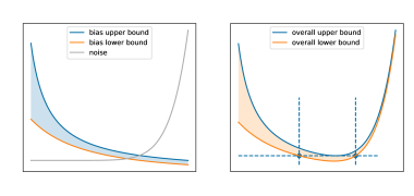
Figure 8: Left: Rough upper and lower bounds for the bias term (shaded region), along with the noise variance (gray). Right: Overall upper and lower bound for the in-context loss. The horizontal dashed line establishes an upper bound for the optimal loss, while the vertical dashed lines establish lower and upper bounds for the parameter $w_{KQ}$ that can attain the optimal loss.

For the nonlinear function class $\operatorname{\mathcal{F}}_{L}^{+}$, we have the following.

Theorem E.1.

Suppose the functions seen in pretraining are drawn from $D(\operatorname{\mathcal{F}}_{L}^{+})$ as in Definition 3.2, the covariates are drawn as Assumption 3.3, and the noise variance $\sigma^{2}$ satisfies $dn^{\frac{d}{2}}\geq\frac{L^{2}}{\sigma^{2}}\geq\frac{1}{n}$, and $n^{\frac{2}{d}}\geq\Omega(1)$, then the optimal $\mathbf{M}$ satisfies

$$\mathbf{M}=w_{KQ}\mathbf{I}_{d}$$ (15)

where $w_{KQ}$ satisfies

$$\Omega\left(\left(nL^{2}\right)^{\frac{1}{d+2}}\right)\leq w_{KQ}\leq\operatorname{\mathcal{O}}\left(\left(nL^{2}\right)^{\frac{2}{d+2}}\right).$$ (16)

Proof.

By combining Lemmas C.8, C.9, and D.1 , we obtain the following overall bound on the loss, provided $r^{\frac{d}{2}}\leq\frac{1}{45\sqrt{d}}\frac{n}{\log n}$:

$$\underline{c}\left(\frac{L^{2}}{\left(w_{KQ}+1\right)^{2}}+\frac{\sigma^{2}w_{KQ}^{\frac{d}{2}}}{n}\right)\leq\operatorname{\mathcal{L}}(w_{KQ})\leq\overline{c}\left(\frac{L^{2}}{w_{KQ}}+\sigma^{2}\frac{w_{KQ}^{\frac{d}{2}}}{n}+\frac{\sigma^{2}+L^{2}}{n}\right)$$

for some constants $\overline{c},\underline{c}$ that only depend on $d$. In the range $w_{KQ}\geq\frac{d+\sqrt{d}}{2}$, the upper bound is minimized at $w_{KQ}=\left(\frac{nL^{2}}{\sigma^{2}d}\right)^{\frac{2}{d+2}}$. We will assume that $n$ is large enough that this exceeds the lower bound established in Lemma C.9 for $w_{KQ}\leq\frac{d+\sqrt{d}}{2}$.

$$\operatorname{\mathcal{L}_{\text{noise}}}(w_{KQ})\leq\overline{c}\left(L^{2}\left(\frac{\sigma^{2}d}{nL^{2}}\right)^{\frac{2}{d+2}}+\frac{\sigma^{2}+L^{2}}{n}\right)$$

For $dn^{\frac{d}{2}}\geq\frac{L^{2}}{\sigma^{2}}\geq\frac{1}{n}$, we see that the first term is largest of the three

$$\operatorname{\mathcal{L}_{\text{noise}}}(w_{KQ})\leq\overline{3}cL^{2}\left(\frac{\sigma^{2}d}{nL^{2}}\right)^{\frac{2}{d+2}}$$

From Lemma C.9 we have $\operatorname{\mathcal{L}_{\text{noise}}}(w_{KQ})\geq\frac{L^{2}}{w_{KQ}^{2}}+\sigma^{2}\frac{w_{KQ}^{\frac{d}{2}}}{n}\geq\frac{L^{2}}{w_{KQ}^{2}}$

$$\underline{c}\frac{L^{2}}{w_{KQ}^{2}}\leq\operatorname{\mathcal{L}_{\text{noise}}}(w_{KQ})\leq 3\overline{c}L^{2}\left(\frac{\sigma^{2}d}{nL^{2}}\right)^{\frac{2}{d+2}}$$

$$\implies \left(\frac{nL^{2}}{d\sigma^{2}}\right)^{\frac{1}{d+2}}\sqrt{\frac{\underline{c}}{3\overline{c}}}\leq w_{KQ}$$

for the upper bound, we similarly also have

$$\frac{L^{2}}{w_{KQ}^{2}}+\sigma^{2}\frac{w_{KQ}^{\frac{d}{2}}}{n}\geq\sigma^{2}\frac{w_{KQ}^{\frac{d}{2}}}{n}$$

$$\implies w_{KQ}\leq\left(\frac{nL^{2}}{\sigma^{2}}\right)^{\frac{2}{d+2}}\left(2\frac{\overline{c}}{\underline{c}}d^{\frac{2}{d+2}}\right)^{\frac{2}{d}}$$

Of course, for this to not be vacuous we need

$$\left(\frac{nL^{2}}{\sigma^{2}}\right)^{\frac{2}{d+2}}\left(2\frac{\overline{c}}{\underline{c}}d^{\frac{2}{d+2}}\right)^{\frac{2}{d}}\leq\left(\frac{1}{45\sqrt{d}}\frac{n}{\log n}\right)^{\frac{2}{d}}.$$

We will again hide constants that depend only on $d$ and write this as

$$c_{1}\left(\frac{nL^{2}}{\sigma^{2}}\right)^{\frac{2}{d+2}}\leq c_{2}\left(\frac{n}{\log n}\right)^{\frac{2}{d}}$$

which is true for large enough $n$ since the $\log$ grows slower than any polynomial. ∎

For the affine function class $\operatorname{\mathcal{F}}^{\text{aff}}_{L}$, we have the following

Theorem E.2.

If the functions seen in pretraining are drawn from $D(\operatorname{\mathcal{F}}^{\text{aff}}_{L})$ as in Definition 3.2, and the noise variance $\sigma^{2}$ satisfies $n^{\frac{2}{d+2}}\geq\frac{L^{2}}{\sigma^{2}}\geq\frac{1}{n}$, and $n^{\frac{2}{d}}\geq\Omega(1)$, and the covariates are drawn as Assumption 3.3, the optimal $\mathbf{M}$ satisfies

$$\mathbf{M}=w_{KQ}\mathbf{I}_{d}$$ (17)

where $w_{KQ}$ satisfies

$$\Omega\left(\left(nL^{2}\right)^{\frac{1}{d+4}}\right)\leq w_{KQ}\leq\operatorname{\mathcal{O}}\left(\left(nL^{2}\right)^{\frac{2(d+2)}{d(d+4)}}\right).$$ (18)

Proof.

The overall bound on the loss, provided $r^{\frac{d}{2}}\leq\frac{1}{45\sqrt{d}}\frac{n}{\log n}$, combining Lemmas C.4, C.5, D.1 is

$$\underline{c}\left(\frac{L^{2}}{\left(w_{KQ}+1\right)^{2}}+\sigma^{2}\frac{w_{KQ}^{\frac{d}{2}}}{n}\right)\leq\operatorname{\mathcal{L}}(w_{KQ})\leq\overline{c}\left(\frac{L^{2}}{w_{KQ}^{2}}+\sigma^{2}\frac{w_{KQ}^{\frac{d}{2}}}{n}+L^{2}\frac{w_{KQ}^{\frac{d}{2}-1}}{n}+\frac{L^{2}+\sigma^{2}}{n}\right)$$

We will minimize the upper bound. First suppose $\frac{L^{2}}{\sigma^{2}}\geq w_{KQ}$ for the $w_{KQ}$ that minimizes the upper bound. Then we have

$$\operatorname{\mathcal{L}}(w_{KQ})\leq\overline{c}\left(\frac{L^{2}}{w_{KQ}^{2}}+\frac{\sigma^{2}}{n}+2L^{2}\frac{w_{KQ}^{\frac{d}{2}-1}}{n}\right)$$

This upper bound is minimized at $w_{KQ}=n^{\frac{2}{d+2}}$. However, this contradicts the constraint that $w_{KQ}\leq\frac{L^{2}}{\sigma^{2}}$, when $n^{\frac{2}{d+2}}\geq\frac{L^{2}}{\sigma^{2}}$, as we assume. So we have $w_{KQ}\geq\frac{L^{2}}{\sigma^{2}}$ for the minimizer. This means the upper bound is no more than

$$\operatorname{\mathcal{L}}(w_{KQ})\leq\overline{c}\left(\frac{L^{2}}{w_{KQ}^{2}}+\sigma^{2}\frac{2w_{KQ}^{\frac{d}{2}}}{n}+\frac{\sigma^{2}+L^{2}}{n}\right)$$

This upper bound is minimized at $w_{KQ}=\left(\frac{nL^{2}}{\sigma^{2}d}\right)^{\frac{2}{d+4}}$. We will assume that $n$ is large enough that this exceeds the lower bound established in Lemma C.5 for $w_{KQ}\leq\frac{d+\sqrt{d}}{2}$. Under the conditions $n>\frac{d}{2}\left(\frac{L^{2}}{\sigma^{2}}\right)^{\frac{4}{d}},\frac{d\sigma^{2}}{2L^{2}}$ we have that

$$\operatorname{\mathcal{L}_{\text{noise}}}(w_{KQ})\leq 5L^{2}\overline{c}\left(\frac{\sigma^{2}d}{nL^{2}}\right)^{\frac{2}{d+4}}$$

We see that

$$\underline{c}\left(\frac{L^{2}}{w_{KQ}^{2}}+\sigma^{2}\frac{w_{KQ}^{\frac{d}{2}}}{n}\right)\geq\underline{c}\frac{L^{2}}{w_{KQ}^{2}}$$

$$\implies \underline{c}\frac{L^{2}}{w_{KQ}^{2}}\leq 5L^{2}\overline{c}\left(\frac{\sigma^{2}d}{nL^{2}}\right)^{\frac{2}{d+4}}$$

$$\implies \left(\frac{nL^{2}}{\sigma^{2}}\right)^{\frac{1}{d+4}}\sqrt{\frac{\underline{c}}{5\overline{c}}}\left(\frac{1}{d}\right)^{\frac{1}{d+4}}\leq w_{KQ}$$

for the upper bound, we similarly also have

$$\underline{c}\left(\frac{L^{2}}{w_{KQ}^{2}}+\sigma^{2}\frac{w_{KQ}^{\frac{d}{2}}}{n}\right)\geq\underline{c}\sigma^{2}\frac{w_{KQ}^{\frac{d}{2}}}{n}$$

$$\implies w_{KQ}\leq\left(\frac{nL^{2}}{\sigma^{2}}\right)^{\frac{2(d+2)}{d(d+4)}}\left(5\frac{\overline{c}}{\underline{c}}d^{\frac{2}{d+4}}\right)^{\frac{2}{d}}$$

Of course, for this to not be vacuous we need

$$\left(\frac{nL^{2}}{\sigma^{2}}\right)^{\frac{2(d+2)}{d(d+4)}}\left(5\frac{\overline{c}}{\underline{c}}d^{\frac{2}{d+4}}\right)^{\frac{2}{d}}\leq\left(\frac{1}{45\sqrt{d}}\frac{n}{\log n}\right)^{\frac{2}{d}}.$$

We will again hide constants that depend only on $d$ and write this as

$$c_{1}\left(\frac{nL^{2}}{\sigma^{2}}\right)^{\frac{2(d+2)}{d(d+4)}}\leq c_{2}\left(\frac{n}{\log n}\right)^{\frac{2}{d}}$$

which again is true for large enough $n$ since the $\log$ grows slower than any polynomial. ∎

E.1 Generalization Bounds

We conclude this section with a proof of the generalization error on a new $L-$Lipschitz task.

Theorem E.3.

Suppose our attention is first pretrained on tasks drawn from $D(\operatorname{\mathcal{F}}_{L}^{+})$ and then tested on an arbitrary $L-$Lipschitz task, then the loss on the new task is upper bounded as $\operatorname{\mathcal{L}}\leq\operatorname{\mathcal{O}}\left(\frac{L^{2}}{\Lambda^{\beta}}\right).$ Furthermore, if the new task is instead drawn from $D(\operatorname{\mathcal{F}}_{L^{\prime}}^{+})$, the loss is lower bounded as $\operatorname{\mathcal{L}}\geq\min\{\Omega(\frac{L^{\prime 2}}{\Lambda^{2\beta}}),\Omega(\frac{\Lambda^{\beta d/2}}{n})\}$

Proof.

We know from Theorem E.2 that $\Omega(\Lambda^{\beta})\leq w_{KQ}\leq\operatorname{\mathcal{O}}(\Lambda^{2\beta})$. The upper bound for $\operatorname{\mathcal{L}}(w_{KQ})$, which is $\operatorname{\mathcal{O}}(\frac{L^{2}}{w_{KQ}}+\frac{w_{KQ}^{\frac{d}{2}}}{n})$, is a convex function for $d\geq 2$, so in any range it attains its maximum value at the extreme points. We can check the cases to see that this is $\operatorname{\mathcal{O}}(\max\{\frac{L^{2}}{\Lambda^{\beta}}+\frac{\Lambda^{d\beta/2}}{n},\frac{L^{2}}{\Lambda^{2\beta}}+\frac{\Lambda^{d\beta}}{n}\})=\operatorname{\mathcal{O}}(\frac{L^{2}}{\Lambda^{\beta}}+\frac{\Lambda^{d\beta/2}}{n}+\frac{L^{2}}{\Lambda^{2\beta}}+\frac{\Lambda^{d\beta}}{n})=\operatorname{\mathcal{O}}(\frac{L^{2}}{\Lambda^{\beta}})$ for large enough $n$.

Now consider testing on a new task from $D(F_{L^{\prime}}^{+})$. The ICL loss for $\Omega\left(\Lambda^{\beta}\right)\leq w_{KQ}\leq\operatorname{\mathcal{O}}\left(\Lambda^{2\beta}\right)$ is bounded below as $\Omega(\frac{L^{\prime 2}}{\Lambda^{2\beta}})$ and $\Omega(\frac{\Lambda^{\beta d/2}}{n})$. ∎

The implication of this is that if $L^{\prime}\gg L$, the error scales as $\left(L^{\prime}\right)^{2}$ rather than $\left(L^{\prime}\right)^{\frac{2d}{d+2}}$ while for $L^{\prime}\ll L$, the error is lower bounded by a constant.

Appendix F Lower Bound for Linear Attention

In this section we prove Theorem 3.6.

Lemma F.1.

Consider the function distributions $D(\operatorname{\mathcal{F}}_{L})$ and $D(\operatorname{\mathcal{F}}_{L}^{+})$ described in Definition 3.2. We have $\mathcal{L}_{LA}\geq\Omega(L^{2})$, that is, the ICL error is lower bounded as $\Omega(L^{2})$.

Proof.

We start by decomposing the ICL loss into a bias dependent term and a cenetered term. For $f=\in\operatorname{\mathcal{F}}_{L}$ or $\operatorname{\mathcal{F}}_{L}^{+}$, let $\overline{f}$ denote the centered function $f-\operatorname{\mathbb{E}}_{\operatorname{{\bf\it x}}}f$. Let $f^{\prime}$ denote the flip of $f$ about its expected value, so $f^{\prime}=\operatorname{\mathbb{E}}_{x}f-\overline{f}$. We observe that $\overline{f}$ is independent of $\operatorname{\mathbb{E}}_{x}f$. For linear attention, we have, for $f\sim D(\mathcal{F})$

$$\mathcal{L}_{\text{LA}}(\mathbf{M}) =\operatorname{\mathbb{E}}_{f,\{\operatorname{{\bf\it x}}_{i}\}_{i},\{\epsilon_{i}\}_{i}}\left[\left(h_{LA}(\operatorname{{\bf\it x}}_{n+1})-f(\operatorname{{\bf\it x}}_{n+1})\right)^{2}\right]$$

$$=\operatorname{\mathbb{E}}_{f,\{\operatorname{{\bf\it x}}_{i}\}_{i},\{\epsilon_{i}\}_{i}}\left[\left(\sum_{i=1}^{n}\left((f(\operatorname{{\bf\it x}}_{i})+\epsilon_{i}){\operatorname{{\bf\it x}}_{i}^{\top}\mathbf{M}\operatorname{{\bf\it x}}_{n+1}}\right)-f(\operatorname{{\bf\it x}}_{n+1})\right)^{2}\right]$$

$$=\operatorname{\mathbb{E}}_{f,\{\operatorname{{\bf\it x}}_{i}\}_{i},\{\epsilon_{i}\}_{i}}\left[\left(\sum_{i=1}^{n}\left(\overline{f}(\operatorname{{\bf\it x}}_{i}){\operatorname{{\bf\it x}}_{i}^{\top}\mathbf{M}\operatorname{{\bf\it x}}_{n+1}}+\epsilon_{i}{\operatorname{{\bf\it x}}_{i}^{\top}\mathbf{M}\operatorname{{\bf\it x}}_{n+1}}+\operatorname{\mathbb{E}}_{x}f{\operatorname{{\bf\it x}}_{i}^{\top}\mathbf{M}\operatorname{{\bf\it x}}_{n+1}}\right)-f(\operatorname{{\bf\it x}}_{n+1})\right)^{2}\right]$$

$$=\operatorname{\mathbb{E}}_{f,\{\operatorname{{\bf\it x}}_{i}\}_{i},\{\epsilon_{i}\}_{i}}\left[\left(\sum_{i=1}^{n}\left(\overline{f}(\operatorname{{\bf\it x}}_{i}){\operatorname{{\bf\it x}}_{i}^{\top}\mathbf{M}\operatorname{{\bf\it x}}_{n+1}}+\epsilon_{i}{\operatorname{{\bf\it x}}_{i}^{\top}\mathbf{M}\operatorname{{\bf\it x}}_{n+1}}\right)-f(\operatorname{{\bf\it x}}_{n+1})\right)^{2}\right]$$ (19)

$$\hskip 28.45274pt+\operatorname{\mathbb{E}}_{f,\operatorname{{\bf\it x}},\{\operatorname{{\bf\it x}}_{i}\}}\left[\left(\sum_{i}\left(\operatorname{\mathbb{E}}_{x}f\right)\operatorname{{\bf\it x}}_{i}^{\top}\mathbf{M}\operatorname{{\bf\it x}}_{n+1}\right)^{2}\right]$$

$$\geq\operatorname{\mathbb{E}}_{f,\{\operatorname{{\bf\it x}}_{i}\}_{i},\{\epsilon_{i}\}_{i}}\left[\left(\sum_{i=1}^{n}\left(\overline{f}(\operatorname{{\bf\it x}}_{i}){\operatorname{{\bf\it x}}_{i}^{\top}\mathbf{M}\operatorname{{\bf\it x}}_{n+1}}+\epsilon_{i}{\operatorname{{\bf\it x}}_{i}^{\top}\mathbf{M}\operatorname{{\bf\it x}}_{n+1}}\right)-\overline{f}(\operatorname{{\bf\it x}}_{n+1})-\operatorname{\mathbb{E}}_{x}f\right)^{2}\right]$$ (20)

By symmetry, this is also equal to the same expression using $f^{\prime}$ instead of $f$, since $f$ and $f^{\prime}$ are distributed identically. Besides, $\operatorname{\mathbb{E}}_{x}f=\operatorname{\mathbb{E}}_{x}f^{\prime}$ and $\epsilon$ is symmetric about the origin, so

$$\mathcal{L}_{\text{LA}}(\mathbf{M}) \geq\operatorname{\mathbb{E}}_{f,\{\operatorname{{\bf\it x}}_{i}\}_{i},\{\epsilon_{i}\}_{i}}\left[\left(\sum_{i=1}^{n}\left(f^{\prime}(\operatorname{{\bf\it x}}_{i}){\operatorname{{\bf\it x}}_{i}^{\top}\mathbf{M}\operatorname{{\bf\it x}}_{n+1}}+\epsilon_{i}{\operatorname{{\bf\it x}}_{i}^{\top}\mathbf{M}\operatorname{{\bf\it x}}_{n+1}}\right)-f^{\prime}(\operatorname{{\bf\it x}}_{n+1})-\operatorname{\mathbb{E}}_{x}f^{\prime}\right)^{2}\right]$$

$$=\operatorname{\mathbb{E}}_{f,\{\operatorname{{\bf\it x}}_{i}\}_{i},\{\epsilon_{i}\}_{i}}\left[\left(\sum_{i=1}^{n}\left(f^{\prime}(\operatorname{{\bf\it x}}_{i}){\operatorname{{\bf\it x}}_{i}^{\top}\mathbf{M}\operatorname{{\bf\it x}}_{n+1}}-\epsilon_{i}{\operatorname{{\bf\it x}}_{i}^{\top}\mathbf{M}\operatorname{{\bf\it x}}_{n+1}}\right)-f^{\prime}(\operatorname{{\bf\it x}}_{n+1})-\operatorname{\mathbb{E}}_{x}f\right)^{2}\right]$$

$$=\operatorname{\mathbb{E}}_{f,\{\operatorname{{\bf\it x}}_{i}\}_{i},\{\epsilon_{i}\}_{i}}\left[\left(-\left(\sum_{i=1}^{n}\left(\overline{f}(\operatorname{{\bf\it x}}_{i}){\operatorname{{\bf\it x}}_{i}^{\top}\mathbf{M}\operatorname{{\bf\it x}}_{n+1}}+\epsilon_{i}{\operatorname{{\bf\it x}}_{i}^{\top}\mathbf{M}\operatorname{{\bf\it x}}_{n+1}}\right)-\overline{f}(\operatorname{{\bf\it x}}_{n+1})\right)-\operatorname{\mathbb{E}}_{x}f\right)^{2}\right]$$

Let $A=\sum_{i=1}^{n}\left(\overline{f}(\operatorname{{\bf\it x}}_{i}){\operatorname{{\bf\it x}}_{i}^{\top}\mathbf{M}\operatorname{{\bf\it x}}_{n+1}}+\epsilon_{i}{\operatorname{{\bf\it x}}_{i}^{\top}\mathbf{M}\operatorname{{\bf\it x}}_{n+1}}\right)-\overline{f}(\operatorname{{\bf\it x}}_{n+1})$ and $B=\operatorname{\mathbb{E}}_{x}f$. Then we see that $\operatorname{\mathcal{L}}_{LA}(\mathbf{M})\geq\frac{1}{2}\operatorname{\mathbb{E}}(A+B)^{2}+\frac{1}{2}\operatorname{\mathbb{E}}(-A+B)^{2}=\operatorname{\mathbb{E}}A^{2}+\operatorname{\mathbb{E}}B^{2}$. Meanwhile, $\operatorname{\mathbb{E}}\left(\operatorname{\mathbb{E}}_{x}f\right)^{2}$ is just the variance of the bias term in $D(\operatorname{\mathcal{F}}_{L})$ or $D(\operatorname{\mathcal{F}}_{L}^{+})$, which is $\frac{L^{2}}{3}$. So $\operatorname{\mathcal{L}}_{LA}(\mathbf{M})\geq\frac{L^{2}}{3}$ ∎

Appendix G Attention Window Captures Appropriate Directions

In this section we prove Theorem 4.4, which entails showing that if the Lipschitzness of the function class is zero in some directions, one-layer self-attention learns to ignore these directions when the function class consists of linear functions.

Lemma G.1.

For any $\mathbf{u}\in\mathbb{S}^{k-1}$ and $\alpha_{1},\dots,\alpha_{n}$ such that $\min_{i}\alpha_{i}>0$, and any $c_{\mathbf{a}},c_{u}\in\mathbb{R}\setminus\{0\}$, define

$$J(c) :=c_{\mathbf{a}}^{2}c_{u}^{2}\mathbb{E}_{\{\mathbf{u}_{i}\}_{i\in[n]}}\left[\frac{\sum_{i=1}^{n}\sum_{j=1}^{n}(\mathbf{u}_{i}-\mathbf{u})^{\top}(\mathbf{u}_{j}-\mathbf{u})e^{c_{u}^{2}c\mathbf{u}_{i}^{\top}\mathbf{u}+c_{u}^{2}c\mathbf{u}_{j}^{\top}\mathbf{u}}\alpha_{i}\alpha_{j}}{(\sum_{i=1}^{n}e^{c_{u}^{2}c\mathbf{u}_{i}^{\top}\mathbf{u}}\alpha_{i})^{2}}\right]$$

$$\quad+\sigma^{2}\mathbb{E}_{\{\mathbf{u}_{i}\}_{i\in[n]}}\left[\frac{\sum_{i=1}^{n}e^{2c_{u}^{2}c\mathbf{u}_{i}^{\top}\mathbf{u}}\alpha_{i}^{2}}{(\sum_{i=1}^{n}e^{c_{u}^{2}c\mathbf{u}_{i}^{\top}\mathbf{u}}\alpha_{i})^{2}}\right]$$

Then for any $\delta>0$, $0\notin\arg\min_{0\leq c\leq\delta}J(c)$.

Proof.

We show that there exists some arbitrarily small $\epsilon>0$ such that $J(\epsilon)<J(0)$ by showing $\frac{dJ(c)}{dc}\big{|}_{c=0}<0$. We have

$$\frac{dJ(c)}{dc}$$

$$=2c_{u}^{4}\mathbb{E}_{\{\mathbf{u}_{i}\}_{i\in[n]}}\Bigg{[}\sum_{i=1}^{n}\sum_{i^{\prime}=1}^{n}\sum_{i^{\prime\prime}=1}^{n}(\mathbf{u}_{i}-\mathbf{u})^{\top}(\mathbf{u}_{i^{\prime}}-\mathbf{u})(\mathbf{u}_{i}^{\top}\mathbf{u}-\mathbf{u}_{i^{\prime\prime}}^{\top}\mathbf{u})\frac{e^{c_{u}^{2}c(\mathbf{u}_{i}+\mathbf{u}_{i^{\prime}}+\mathbf{u}_{i^{\prime\prime}})^{\top}u}\alpha_{i}\alpha_{i^{\prime}}\alpha_{i^{\prime\prime}}}{(\sum_{i=1}^{n}e^{c_{u}^{2}c\mathbf{u}_{i}^{\top}\mathbf{u}}\alpha_{i})^{3}}\Bigg{]}$$

$$\quad+2\sigma^{2}c_{u}^{2}\mathbb{E}_{\{\mathbf{u}_{i}\}_{i\in[n]}}\Bigg{[}\sum_{i=1}^{n}\sum_{i^{\prime}=1}^{n}\sum_{i^{\prime\prime}=1}^{n}(\mathbf{u}_{i}^{\top}\mathbf{u}-\mathbf{u}_{i^{\prime}}^{\top}\mathbf{u})\frac{e^{c_{u}^{2}c(2\mathbf{u}_{i}+\mathbf{u}_{i^{\prime}}+\mathbf{u}_{i^{\prime\prime}})^{\top}\mathbf{u}}\alpha_{i}^{2}\alpha_{i^{\prime}}\alpha_{i^{\prime\prime}}}{(\sum_{i=1}^{n}e^{c_{u}^{2}c\mathbf{u}_{i}^{\top}\mathbf{u}}\alpha_{i})^{4}}\Bigg{]}$$

Setting $c=0$ results in

$$\frac{dJ(c)}{dc}\bigg{|}_{c=0} =\frac{2c_{\mathbf{a}}^{2}c_{u}^{4}}{(\sum_{i=1}^{n}\alpha_{i})^{3}}\sum_{i=1}^{n}\sum_{i^{\prime}=1}^{n}\sum_{i^{\prime\prime}=1}^{n}\mathbb{E}_{\{\mathbf{u}_{i}\}_{i\in[n]}}\left[(\mathbf{u}_{i}-\mathbf{u})^{\top}(\mathbf{u}_{i^{\prime}}-\mathbf{u})(\mathbf{u}_{i}^{\top}\mathbf{u}-\mathbf{u}_{i^{\prime\prime}}^{\top}\mathbf{u})\alpha_{i}\alpha_{i^{\prime}}\alpha_{i^{\prime\prime}}\right]$$

$$\quad+\frac{2\sigma^{2}c_{u}^{2}}{(\sum_{i=1}^{n}\alpha_{i})^{4}}\sum_{i=1}^{n}\sum_{i^{\prime}=1}^{n}\sum_{i^{\prime\prime}=1}^{n}\mathbb{E}_{\{\mathbf{u}_{i}\}_{i\in[n]}}\Bigg{[}(\mathbf{u}_{i}^{\top}\mathbf{u}-\mathbf{u}_{i^{\prime}}^{\top}\mathbf{u})\alpha_{i}^{2}\alpha_{i^{\prime}}\alpha_{i^{\prime\prime}}\Bigg{]}$$

$$=\frac{2c_{\mathbf{a}}^{2}c_{u}^{4}}{(\sum_{i=1}^{n}\alpha_{i})^{3}}\sum_{i=1}^{n}\sum_{i^{\prime}=1}^{n}\sum_{i^{\prime\prime}=1}^{n}\mathbb{E}_{\{\mathbf{u}_{i}\}_{i\in[n]}}\left[(\mathbf{u}_{i}-\mathbf{u})^{\top}(\mathbf{u}_{i^{\prime}}-\mathbf{u})(\mathbf{u}_{i}^{\top}\mathbf{u}-\mathbf{u}_{i^{\prime\prime}}^{\top}\mathbf{u})\alpha_{i}\alpha_{i^{\prime}}\alpha_{i^{\prime\prime}}\right]$$ (21)

$$=\frac{2c_{\mathbf{a}}^{2}c_{u}^{4}}{(\sum_{i=1}^{n}\alpha_{i})^{3}}\sum_{i=1}^{n}\sum_{i^{\prime}=1}^{n}\sum_{i^{\prime\prime}=1}^{n}\mathbb{E}_{\{\mathbf{u}_{i}\}_{i\in[n]}}\left[\left(\mathbf{u}_{i}^{\top}\mathbf{u}_{i^{\prime}}+1\right)(\mathbf{u}_{i}^{\top}\mathbf{u}-\mathbf{u}_{i^{\prime\prime}}^{\top}\mathbf{u})\alpha_{i}\alpha_{i^{\prime}}\alpha_{i^{\prime\prime}}\right]$$

$$\quad-\frac{2c_{u}^{4}}{(\sum_{i=1}^{n}\alpha_{i})^{3}}\sum_{i=1}^{n}\sum_{i^{\prime}=1}^{n}\sum_{i^{\prime\prime}=1}^{n}\mathbb{E}_{\{\mathbf{u}_{i}\}_{i\in[n]}}\left[(\mathbf{u}^{\top}\mathbf{u}_{i^{\prime}}+\mathbf{u}_{i}^{\top}\mathbf{u})(\mathbf{u}_{i}^{\top}\mathbf{u}-\mathbf{u}_{i^{\prime\prime}}^{\top}\mathbf{u})\alpha_{i}\alpha_{i^{\prime}}\alpha_{i^{\prime\prime}}\right]$$

$$=-\frac{2c_{\mathbf{a}}^{2}c_{u}^{4}}{(\sum_{i=1}^{n}\alpha_{i})^{3}}$$

$$\quad\quad\times\sum_{i=1}^{n}\sum_{i^{\prime}=1}^{n}\sum_{i^{\prime\prime}=1}^{n}\mathbb{E}_{\{\mathbf{u}_{i}\}_{i\in[n]}}\left[(\mathbf{u}^{\top}\mathbf{u}_{i^{\prime}}+\mathbf{u}_{i}^{\top}\mathbf{u})(\mathbf{u}_{i}^{\top}\mathbf{u}-\mathbf{u}_{i^{\prime\prime}}^{\top}\mathbf{u})\alpha_{i}\alpha_{i^{\prime}}\alpha_{i^{\prime\prime}}\right]$$ (22)

$$=-\frac{2c_{\mathbf{a}}^{2}c_{u}^{4}}{(\sum_{i=1}^{n}\alpha_{i})^{3}}\sum_{i^{\prime}=1}^{n}\alpha_{i^{\prime}}$$

$$\quad\times\left(\sum_{i=1}^{n}\sum_{i^{\prime\prime}=1}^{n}\mathbb{E}_{\{\mathbf{u}_{i}\}_{i\in[n]}}\left[\mathbf{u}^{\top}\mathbf{u}_{i^{\prime}}\mathbf{u}_{i}^{\top}\mathbf{u}\alpha_{i}\alpha_{i^{\prime\prime}}\right]-\sum_{i=1}^{n}\sum_{i^{\prime\prime}=1}^{n}\mathbb{E}_{\{\mathbf{u}_{i}\}_{i\in[n]}}\left[\mathbf{u}^{\top}\mathbf{u}_{i^{\prime}}\mathbf{u}_{i^{\prime\prime}}^{\top}\mathbf{u}\alpha_{i}\alpha_{i^{\prime\prime}}\right]\right)$$

$$\quad-\frac{2c_{\mathbf{a}}^{2}c_{u}^{4}}{(\sum_{i=1}^{n}\alpha_{i})^{3}}\sum_{i=1}^{n}\sum_{i^{\prime}=1}^{n}\sum_{i^{\prime\prime}=1}^{n}\mathbb{E}_{\{\mathbf{u}_{i}\}_{i\in[n]}}\left[\mathbf{u}_{i}^{\top}\mathbf{u}(\mathbf{u}_{i}^{\top}\mathbf{u}-\mathbf{u}_{i^{\prime\prime}}^{\top}\mathbf{u})\alpha_{i}\alpha_{i^{\prime}}\alpha_{i^{\prime\prime}}\right]$$

$$=-\frac{2c_{\mathbf{a}}^{2}c_{u}^{4}}{(\sum_{i=1}^{n}\alpha_{i})^{3}}\sum_{i=1}^{n}\sum_{i^{\prime}=1}^{n}\sum_{i^{\prime\prime}=1}^{n}\mathbb{E}_{\{\mathbf{u}_{i}\}_{i\in[n]}}\left[\mathbf{u}_{i}^{\top}\mathbf{u}(\mathbf{u}_{i}^{\top}\mathbf{u}-\mathbf{u}_{i^{\prime\prime}}^{\top}\mathbf{u})\alpha_{i}\alpha_{i^{\prime}}\alpha_{i^{\prime\prime}}\right]$$ (23)

$$=-\frac{2c_{\mathbf{a}}^{2}c_{u}^{4}}{(\sum_{i=1}^{n}\alpha_{i})^{3}}\sum_{i=1}^{n}\sum_{i^{\prime}=1}^{n}\sum_{i^{\prime\prime}=1}^{n}\alpha_{i}\alpha_{i^{\prime}}\alpha_{i^{\prime\prime}}\mathbb{E}_{\{\mathbf{u}_{i}\}_{i\in[n]}}\left[\mathbf{u}^{\top}\mathbf{u}_{i}\mathbf{u}_{i}^{\top}\mathbf{u}\right]$$

$$\quad+\frac{2c_{\mathbf{a}}^{2}c_{u}^{4}}{(\sum_{i=1}^{n}\alpha_{i})^{3}}\sum_{i=1}^{n}\sum_{i^{\prime}=1}^{n}\sum_{i^{\prime\prime}=1}^{n}\alpha_{i}\alpha_{i^{\prime}}\alpha_{i^{\prime\prime}}\mathbb{E}_{\{\mathbf{u}_{i}\}_{i\in[n]}}\left[\mathbf{u}^{\top}\mathbf{u}_{i}\mathbf{u}_{i^{\prime\prime}}^{\top}\mathbf{u}\right]$$

$$=-\frac{2c_{\mathbf{a}}^{2}c_{u}^{4}}{k}+\frac{2c_{u}^{4}}{k(\sum_{i=1}^{n}\alpha_{i})^{3}}\sum_{i=1}^{n}\sum_{i^{\prime}=1}^{n}\alpha_{i}^{2}\alpha_{i^{\prime}}$$ (24)

$$=-\frac{2c_{\mathbf{a}}^{2}c_{u}^{4}}{k}\left(1-\frac{\sum_{i=1}^{n}\alpha_{i}^{2}}{(\sum_{i=1}^{n}\alpha_{i})^{2}}\right)$$

$$<0$$ (25)

where (21) follows since $\mathbb{E}[\mathbf{u}_{i}]=0$, (22) similarly follows since odd moments of uniform random variables on the hypersphere are zero, (23) follows by the i.i.d.-ness of the $\mathbf{u}_{i}$’s, (24) follows since $\mathbb{E}[\mathbf{u}_{i}\mathbf{u}_{i}^{\top}]=\frac{1}{k}\mathbf{I}_{k}$ and $\mathbf{u}^{\top}\mathbf{u}=1$, and (25) follows since $\min_{i}\alpha_{i}>0$. This completes the proof. ∎

Lemma G.2.

Consider any $\mathbf{B}\in\mathbb{O}^{d\times k}$ and resulting function class $\mathcal{F}_{\mathbf{B}}^{\text{lin}}$. Consider the training population loss $\mathcal{L}$ defined in (ICL), and tasks drawn from $D(\mathcal{F}_{\mathbf{B}}^{\text{lin}})$ such that $\mathbb{E}_{\mathbf{a}}[\mathbf{\mathbf{aa}}^{\top}]=c_{\mathbf{a}}^{2}\mathbf{I}_{k}$ for some $c_{\mathbf{a}}\neq 0$ and let $\mathbf{M}:=\mathbf{M}_{K}^{\top}\mathbf{M}_{Q}$ be optimized over the domain $\mathcal{M}_{\hat{c}}:=\{\mathbf{M}\in\mathbb{R}^{d\times d}:\mathbf{M}=\mathbf{M}^{\top},\|\mathbf{B}^{\top}\mathbf{M}\mathbf{B}\|_{2}\leq\frac{\hat{c}}{c_{u}^{2}}\}$ for some $\hat{c}>0$. Then any

$$\mathbf{M}^{*}\in\arg\min_{\mathbf{M}\in\mathcal{M}_{\hat{c}}}\mathcal{L}(\mathbf{M})$$ (26)

satisfies $\mathbf{M}^{*}={c^{*}}\mathbf{BB}^{T}+\mathbf{B}_{\perp}\mathbf{QB}_{\perp}^{\top}$ for some $c^{*}:|c^{*}|\in(0,\frac{\hat{c}}{c_{u}^{2}}]$ and symmetric matrix $\mathbf{Q}\in\mathbb{R}^{(d-k)\times(d-k)}$.

Proof.

Without loss of generality (WLOG), we can decompose $\mathbf{M}=\mathbf{BPB}^{\top}+\mathbf{B}_{\perp}\mathbf{Q}\mathbf{B}_{\perp}^{\top}$ for some symmetric $\mathbf{P}\in\mathbb{R}^{k\times k}$ such that $\|\mathbf{P}\|_{2}\leq c$ and symmetric $\mathbf{Q}\in\mathbb{R}^{(d-k)\times(d-k)}$. Recall that for each $i\in[n+1]$, $\mathbf{x}_{i}=c_{u}\mathbf{B}\mathbf{u}_{i}+c_{{v}}\mathbf{B}_{\perp}\mathbf{v}_{i}$. Thus, for each $i\in[n]$, we have

$$e^{\mathbf{x}_{i}^{\top}\mathbf{M}\mathbf{x}_{n+1}} =e^{c_{p}\mathbf{x}_{i}^{\top}\mathbf{BPB}^{\top}\mathbf{x}_{n+1}}e^{\mathbf{x}_{i}^{\top}\mathbf{B}_{\perp}\mathbf{QB}_{\perp}^{\top}\mathbf{x}_{n+1}}$$

$$=e^{c_{u}^{2}\mathbf{u}_{i}^{\top}\mathbf{P}\mathbf{u}_{n+1}}e^{\mathbf{v}_{i}^{\top}\mathbf{Qv}_{n+1}}$$

$$=e^{c_{u}^{2}\mathbf{u}_{i}^{\top}\mathbf{P}\mathbf{u}_{n+1}}\alpha_{i}$$ (27)

where, for each $i\in[n]$, $\alpha_{i}\coloneqq e^{c_{{v}}\mathbf{v}_{i}^{\top}\mathbf{Qv}_{n+1}}$. For ease of notation, denote $\mathbf{x}=\mathbf{x}_{n+1}$ and $\mathbf{u}:=\mathbf{u}_{n+1}$. We start by expanding the square and using the linearity of the expectation to re-write the population loss as:

$$\mathcal{L}(\mathbf{M})$$

$$=\mathbb{E}_{\mathbf{a},\mathbf{x},\{\mathbf{x}_{i}\}_{i\in[n]},\{\epsilon_{i}\}_{i\in[n]}}$$

$$\quad\quad\quad\quad\left[\frac{\sum_{i=1}^{n}\sum_{j=1}^{n}(\mathbf{a}^{\top}\mathbf{B}^{\top}\mathbf{x}_{i}-\mathbf{a}^{\top}\mathbf{B}^{\top}\mathbf{x}+\epsilon_{i})(\mathbf{a}^{\top}\mathbf{B}^{\top}\mathbf{x}_{j}-\mathbf{a}^{\top}\mathbf{B}^{\top}\mathbf{x}+\epsilon_{j})e^{\mathbf{x}_{i}^{\top}\mathbf{Mx}+\mathbf{x}_{j}^{\top}\mathbf{Mx}}}{(\sum_{i=1}^{n}e^{\mathbf{x}_{i}^{\top}\mathbf{Mx}})^{2}}\right]$$

$$=c_{\mathbf{a}}^{2}c_{u}^{2}\mathbb{E}_{\mathbf{a},\mathbf{u},\{\mathbf{u}_{i}\}_{i\in[n]},\{\alpha_{i}\}_{i\in[n]}}$$

$$\quad\left[\frac{\sum_{i=1}^{n}\sum_{j=1}^{n}(\mathbf{a}^{\top}\mathbf{B}^{\top}\mathbf{u}_{i}-\mathbf{a}^{\top}\mathbf{B}^{\top}\mathbf{u})(\mathbf{a}^{\top}\mathbf{B}^{\top}\mathbf{u}_{j}-\mathbf{a}^{\top}\mathbf{B}^{\top}\mathbf{u})e^{c_{u}^{2}\mathbf{u}_{i}^{\top}\mathbf{P}\mathbf{u}+c_{u}^{2}\mathbf{u}_{j}^{\top}\mathbf{P}\mathbf{u}}\alpha_{i}\alpha_{j}}{(\sum_{i=1}^{n}e^{c_{u}^{2}\mathbf{u}_{i}^{\top}\mathbf{P}\mathbf{u}}\alpha_{i})^{2}}\right]$$

$$\quad\quad+\sigma^{2}\mathbb{E}_{u,\{\mathbf{u}_{i}\}_{i\in[n]},\{\alpha_{i}\}_{i\in[n]},\{\epsilon_{i}\}_{i\in[n]}}\left[\frac{\sum_{i=1}^{n}e^{2c_{u}^{2}\mathbf{u}_{i}^{\top}\mathbf{P}\mathbf{u}}\alpha_{i}^{2}}{(\sum_{i=1}^{n}e^{c_{u}^{2}\mathbf{u}_{i}^{\top}\mathbf{P}\mathbf{u}}\alpha_{i})^{2}}\right]$$

$$=\mathbb{E}_{u}\Bigg{[}\;\underbrace{c_{\mathbf{a}}^{2}c_{u}^{2}\mathbb{E}_{\{\mathbf{u}_{i}\}_{i\in[n]},\{\alpha_{i}\}_{i\in[n]}}\left[\frac{\sum_{i=1}^{n}\sum_{j=1}^{n}(\mathbf{u}_{i}-u)^{\top}(\mathbf{u}_{j}-\mathbf{u})e^{c_{u}^{2}\mathbf{u}_{i}^{\top}\mathbf{P}\mathbf{u}+c_{u}^{2}\mathbf{u}_{j}^{\top}\mathbf{P}\mathbf{u}}\alpha_{i}\alpha_{j}}{(\sum_{i=1}^{n}e^{c_{u}^{2}\mathbf{u}_{i}^{\top}\mathbf{P}\mathbf{u}}\alpha_{i})^{2}}\right]}_{=:\tilde{\mathcal{L}}_{\text{signal}}(\mathbf{M},\mathbf{u})}$$

$$\quad\quad\quad\quad+\underbrace{\sigma^{2}\mathbb{E}_{x,\{\mathbf{x}_{i}\}_{i\in[n]}}\left[\frac{\sum_{i=1}^{n}e^{2c_{u}^{2}\mathbf{u}_{i}^{\top}\mathbf{P}\mathbf{u}}\alpha_{i}^{2}}{(\sum_{i=1}^{n}e^{c_{u}^{2}\mathbf{u}_{i}^{\top}\mathbf{P}\mathbf{u}}\alpha_{i})^{2}}\right]}_{=:\tilde{\mathcal{L}}_{\text{noise}}(\mathbf{M},\mathbf{u})}\;\Bigg{]}$$ (28)

WLOG we can write $\mathbf{P}\mathbf{u}=\mathbf{R}_{\mathbf{u}}\mathbf{u}\|\mathbf{P}\mathbf{u}\|_{2}$ for some rotation matrix $R_{\mathbf{u}}\in\mathbb{O}^{k\times k}$. Denote $\bar{c}_{\mathbf{u}}:=\|\mathbf{P}\mathbf{u}\|_{2}$. Then we have

$$\tilde{\mathcal{L}}_{\text{signal}}(\mathbf{M},\mathbf{u})$$

$$=c_{\mathbf{a}}^{2}c_{u}^{2}\mathbb{E}_{\{\mathbf{u}_{i}\}_{i},\{\alpha_{i}\}_{i}}\left[\frac{\sum_{i=1}^{n}\sum_{j=1}^{n}(\mathbf{u}_{i}-u)^{\top}(\mathbf{u}_{j}-\mathbf{u})e^{c_{u}^{2}\bar{c}_{u}\mathbf{u}_{i}^{\top}\mathbf{R}_{\mathbf{u}}\mathbf{u}+c_{u}^{2}\bar{c}_{u}\mathbf{u}_{j}^{\top}\mathbf{R}_{\mathbf{u}}\mathbf{u}}\alpha_{i}\alpha_{j}}{(\sum_{i=1}^{n}e^{c_{u}^{2}\bar{c}_{u}\mathbf{u}_{i}^{\top}\mathbf{R}_{\mathbf{u}}\mathbf{u}}\alpha_{i})^{2}}\right]$$

$$=c_{\mathbf{a}}^{2}c_{u}^{2}\mathbb{E}_{\{\mathbf{u}_{i}\}_{i},\{\alpha_{i}\}_{i}}\left[\frac{\sum_{i=1}^{n}\sum_{j=1}^{n}(\mathbf{u}_{i}-u)^{\top}\mathbf{R}_{\mathbf{u}}\mathbf{R}_{\mathbf{u}}^{\top}(\mathbf{u}_{j}-\mathbf{u})e^{c_{u}^{2}\bar{c}_{u}\mathbf{u}_{i}^{\top}\mathbf{R}_{\mathbf{u}}\mathbf{u}+c_{u}^{2}\bar{c}_{u}\mathbf{u}_{j}^{\top}\mathbf{R}_{\mathbf{u}}\mathbf{u}}\alpha_{i}\alpha_{j}}{(\sum_{i=1}^{n}e^{c_{u}^{2}\bar{c}_{u}\mathbf{u}_{i}^{\top}\mathbf{R}_{\mathbf{u}}\mathbf{u}}\alpha_{i})^{2}}\right]$$ (29)

$$=c_{\mathbf{a}}^{2}c_{u}^{2}$$

$$\quad\times\mathbb{E}_{\{\mathbf{u}_{i}\}_{i},\{\alpha_{i}\}_{i}}\left[\frac{\sum_{i=1}^{n}\sum_{j=1}^{n}(\mathbf{R}_{\mathbf{u}}^{\top}\mathbf{u}_{i}-\mathbf{R}_{\mathbf{u}}^{\top}\mathbf{u})^{\top}(\mathbf{R}_{\mathbf{u}}^{\top}\mathbf{u}_{j}-\mathbf{R}_{\mathbf{u}}^{\top}\mathbf{u})e^{c_{u}^{2}\bar{c}_{u}\mathbf{u}_{i}^{\top}\mathbf{R}_{\mathbf{u}}\mathbf{u}+c_{u}^{2}\bar{c}_{u}\mathbf{u}_{j}^{\top}\mathbf{R}_{\mathbf{u}}\mathbf{u}}\alpha_{i}\alpha_{j}}{(\sum_{i=1}^{n}e^{c_{u}^{2}\bar{c}_{u}\mathbf{u}_{i}^{\top}\mathbf{R}_{\mathbf{u}}\mathbf{u}}\alpha_{i})^{2}}\right]$$

$$=c_{\mathbf{a}}^{2}c_{u}^{2}\mathbb{E}_{\{\mathbf{u}_{i}\}_{i},\{\alpha_{i}\}_{i}}\left[\frac{\sum_{i=1}^{n}\sum_{j=1}^{n}(\mathbf{u}_{i}-\mathbf{R}_{\mathbf{u}}^{\top}\mathbf{u})^{\top}(\mathbf{u}_{j}-\mathbf{R}_{\mathbf{u}}^{\top}\mathbf{u})e^{c_{u}^{2}\bar{c}_{u}\mathbf{u}_{i}^{\top}\mathbf{u}+c_{u}^{2}\bar{c}_{u}\mathbf{u}_{j}^{\top}\mathbf{u}}\alpha_{i}\alpha_{j}}{(\sum_{i=1}^{n}e^{c_{u}^{2}\bar{c}_{u}\mathbf{u}_{i}^{\top}\mathbf{u}}\alpha_{i})^{2}}\right]$$ (30)

where (29) follows since $\mathbf{R}_{\mathbf{u}}\mathbf{R}_{\mathbf{u}}^{\top}=\mathbf{I}_{k}$ and (30) follows since the distribution of $\mathbf{u}_{i}$ is the same as the distribution of $\mathbf{R}_{\mathbf{u}}^{\top}\mathbf{u}_{i}$ for any rotation $\mathbf{R}_{\mathbf{u}}^{\top}$. Next, we show that for any $\mathbf{u}$, the loss above can be reduced by setting $\mathbf{R}_{\mathbf{u}}=\mathbf{I}_{k}$. Define

$$g(\mathbf{R},\mathbf{u}):=\mathbb{E}_{\{\mathbf{u}_{i}\}_{i},\{\alpha_{i}\}_{i}}\left[\frac{\sum_{i=1}^{n}\sum_{j=1}^{n}(\mathbf{u}_{i}-\mathbf{R}^{\top}\mathbf{u})^{\top}(\mathbf{u}_{j}-\mathbf{R}^{\top}\mathbf{u})e^{c_{u}^{2}\bar{c}_{u}\mathbf{u}_{i}^{\top}\mathbf{u}+c_{u}^{2}\bar{c}_{u}\mathbf{u}_{j}^{\top}\mathbf{u}}\alpha_{i}\alpha_{j}}{(\sum_{i=1}^{n}e^{c_{u}^{2}\bar{c}_{u}\mathbf{u}_{i}^{\top}\mathbf{u}}\alpha_{i})^{2}}\right]$$ (31)

for any $\mathbf{R}\in\mathbb{O}^{k\times k}$. We have $\mathcal{L}_{\text{signal}}(M)=c_{\mathbf{a}}^{2}c_{u}^{2}\mathbb{E}_{\mathbf{u}}[g(\mathbf{R}_{\mathbf{u}},\mathbf{u})]$, and

$$g(\mathbf{R}_{\mathbf{u}},\mathbf{u})-g(\mathbf{I}_{k},\mathbf{u})$$

$$=\mathbb{E}_{\{\mathbf{u}_{i}\}_{i\in[n]},\{\alpha_{i}\}_{i\in[n]}}\left[\frac{\sum_{i=1}^{n}\sum_{j=1}^{n}(\mathbf{u}_{i}-\mathbf{R}_{\mathbf{u}}^{\top}\mathbf{u})^{\top}(\mathbf{u}_{j}-\mathbf{R}_{\mathbf{u}}^{\top}\mathbf{u})e^{c_{u}^{2}\bar{c}_{u}\mathbf{u}_{i}^{\top}\mathbf{u}+c_{u}^{2}\bar{c}_{u}\mathbf{u}_{j}^{\top}\mathbf{u}}\alpha_{i}\alpha_{j}}{(\sum_{i=1}^{n}e^{c_{u}^{2}\bar{c}_{u}\mathbf{u}_{i}^{\top}\mathbf{u}}\alpha_{i})^{2}}\right]$$

$$\quad\quad-\mathbb{E}_{\{\mathbf{u}_{i}\}_{i\in[n]},\{\alpha_{i}\}_{i\in[n]}}\left[\frac{\sum_{i=1}^{n}\sum_{j=1}^{n}(\mathbf{u}_{i}-\mathbf{u})^{\top}(\mathbf{u}_{j}-\mathbf{u})e^{c_{u}^{2}\bar{c}_{u}\mathbf{u}_{i}^{\top}\mathbf{u}+c_{u}^{2}\bar{c}_{u}\mathbf{u}_{j}^{\top}\mathbf{u}}\alpha_{i}\alpha_{j}}{(\sum_{i=1}^{n}e^{c_{u}^{2}\bar{c}_{u}\mathbf{u}_{i}^{\top}\mathbf{u}}\alpha_{i})^{2}}\right]$$

$$=\mathbb{E}_{\{\mathbf{u}_{i}\}_{i\in[n]},\{\alpha_{i}\}_{i\in[n]}}$$

$$\quad\quad\times\left[\frac{\sum_{i=1}^{n}\sum_{j=1}^{n}(\mathbf{u}_{i}^{\top}\mathbf{u}-\mathbf{u}_{i}^{\top}\mathbf{R}_{\mathbf{u}}^{\top}\mathbf{u}+\mathbf{u}_{j}^{\top}\mathbf{u}-\mathbf{u}_{j}^{\top}\mathbf{R}_{\mathbf{u}}^{\top}\mathbf{u})e^{c_{u}^{2}\bar{c}_{u}\mathbf{u}_{i}^{\top}\mathbf{u}+c_{u}^{2}\bar{c}_{u}\mathbf{u}_{j}^{\top}\mathbf{u}}\alpha_{i}\alpha_{j}}{(\sum_{i=1}^{n}e^{c_{u}^{2}\bar{c}_{u}\mathbf{u}_{i}^{\top}\mathbf{u}}\alpha_{i})^{2}}\right]$$

$$=2\mathbb{E}_{\{\mathbf{u}_{i}\}_{i\in[n]},\{\alpha_{i}\}_{i\in[n]}}\left[\frac{\sum_{i=1}^{n}(\mathbf{u}_{i}^{\top}\mathbf{u}-\mathbf{u}_{i}^{\top}\mathbf{R}_{\mathbf{u}}^{\top}\mathbf{u})e^{c_{u}^{2}\bar{c}_{u}\mathbf{u}_{i}^{\top}\mathbf{u}}\alpha_{i}\sum_{j=1}^{n}e^{c_{u}^{2}\bar{c}_{u}\mathbf{u}_{j}^{\top}\mathbf{u}}\alpha_{j}}{(\sum_{i=1}^{n}e^{c_{u}^{2}\bar{c}_{u}\mathbf{u}_{i}^{\top}\mathbf{u}}\alpha_{i})^{2}}\right]$$

$$=2\mathbb{E}_{\{\mathbf{u}_{i}\}_{i\in[n]},\{\alpha_{i}\}_{i\in[n]}}\left[\frac{\sum_{i=1}^{n}(\mathbf{u}_{i}^{\top}\mathbf{u}-\mathbf{u}_{i}^{\top}\mathbf{R}_{\mathbf{u}}^{\top}\mathbf{u})e^{c_{u}^{2}\bar{c}_{u}\mathbf{u}_{i}^{\top}\mathbf{u}}\alpha_{i}}{\sum_{i=1}^{n}e^{c_{u}^{2}\bar{c}_{u}\mathbf{u}_{i}^{\top}\mathbf{u}}\alpha_{i}}\right]$$

$$=2(\mathbf{u}^{\top}-\mathbf{u}^{\top}\mathbf{R}_{\mathbf{u}})\mathbb{E}_{\{\mathbf{u}_{i}\}_{i\in[n]},\{\alpha_{i}\}_{i\in[n]}}\left[\frac{\sum_{i=1}^{n}\mathbf{u}_{i}e^{c_{u}^{2}\bar{c}_{u}\mathbf{u}_{i}^{\top}\mathbf{u}}\alpha_{i}}{\sum_{i=1}^{n}e^{c_{u}^{2}\bar{c}_{u}\mathbf{u}_{i}^{\top}\mathbf{u}}\alpha_{i}}\right]$$ (32)

Define $\hat{\mathbf{u}}\coloneqq\mathbb{E}_{\{\mathbf{u}_{i}\}_{i\in[n]},\{\alpha_{i}\}_{i\in[n]}}\left[\frac{\sum_{i=1}^{n}\mathbf{u}_{i}e^{c_{u}^{2}\bar{c}_{u}\mathbf{u}_{i}^{\top}\mathbf{u}}\alpha_{i}}{\sum_{i=1}^{n}e^{c_{u}^{2}\bar{c}_{u}\mathbf{u}_{i}^{\top}\mathbf{u}}\alpha_{i}}\right]$ and WLOG write $\mathbf{u}_{i}=\mathbf{p}_{\mathbf{u}_{i}}+\mathbf{q}_{\mathbf{u}_{i}}$, where $\mathbf{p}_{\mathbf{u}_{i}}\coloneqq\mathbf{uu}^{\top}\mathbf{u}_{i}$ and $\mathbf{q}_{\mathbf{u}_{i}}\coloneqq(\mathbf{I}_{k}-\mathbf{uu}^{\top})\mathbf{u}_{i}$. Note that for any $\mathbf{u}_{i}=\mathbf{p}_{\mathbf{u}_{i}}+\mathbf{q}_{\mathbf{u}_{i}}$, $\mathbf{u}_{i}^{\prime}:=\mathbf{p}_{\mathbf{u}_{i}}-\mathbf{q}_{\mathbf{u}_{i}}$ occurs with equal probability, and flipping $\mathbf{q}_{\mathbf{u}_{i}}$ does not change any exponent or $\alpha_{i}$ in (32). Thus

$$\hat{\mathbf{u}} =\mathbb{E}_{\{(\mathbf{p}_{\mathbf{u}_{i}},\mathbf{q}_{\mathbf{u}_{i}})\}_{i\in[n]},\{\alpha_{i}\}_{i\in[n]}}\left[\frac{\sum_{i=1}^{n}(\mathbf{p}_{\mathbf{u}_{i}}+\mathbf{q}_{\mathbf{u}_{i}})e^{c_{u}^{2}\bar{c}_{u}\mathbf{u}_{i}^{\top}\mathbf{u}}\alpha_{i}}{\sum_{i=1}^{n}e^{c_{u}^{2}\bar{c}_{u}\mathbf{u}_{i}^{\top}\mathbf{u}}\alpha_{i}}\right]$$

$$=\tfrac{1}{2}\mathbb{E}_{\{(\mathbf{p}_{\mathbf{u}_{i}},\mathbf{q}_{\mathbf{u}_{i}})\}_{i},\{\alpha_{i}\}_{i}}\left[\frac{\sum_{i=1}^{n}(2\mathbf{p}_{\mathbf{u}_{i}}+\mathbf{q}_{\mathbf{u}_{i}}-\mathbf{q}_{\mathbf{u}_{i}})e^{c_{u}^{2}\bar{c}_{u}\mathbf{u}_{i}^{\top}\mathbf{u}}\alpha_{i}}{\sum_{i=1}^{n}e^{c_{u}^{2}\bar{c}_{u}\mathbf{u}_{i}^{\top}\mathbf{u}}\alpha_{i}}\right]$$

$$=\mathbb{E}_{\{\mathbf{p}_{\mathbf{u}_{i}}\}_{i},\{\alpha_{i}\}_{i}}\left[\frac{\sum_{i=1}^{n}\mathbf{p}_{\mathbf{u}_{i}}e^{c_{u}^{2}\bar{c}_{u}\mathbf{u}_{i}^{\top}\mathbf{u}}\alpha_{i}}{\sum_{i=1}^{n}e^{c_{u}^{2}\bar{c}_{u}\mathbf{u}_{i}^{\top}\mathbf{u}}\alpha_{i}}\right]$$ (33)

$$=\tilde{c}\;\mathbf{u}$$

where $\tilde{c}:=\mathbb{E}_{\{\mathbf{u}_{i}\}_{i\in[n]},\{\alpha_{i}\}_{i\in[n]}}\left[\frac{\sum_{i=1}^{n}\mathbf{u}_{i}^{\top}\mathbf{u}\;e^{c_{u}^{2}\bar{c}_{u}\mathbf{u}_{i}^{\top}\mathbf{u}}\alpha_{i}}{\sum_{i=1}^{n}e^{c_{u}^{2}\bar{c}_{u}\mathbf{u}_{i}^{\top}\mathbf{u}}\alpha_{i}}\right]$. Note that for any $\mathbf{u}_{i}$, $-\mathbf{u}_{i}$ occurs with equal probability, so

$$\tilde{c} =\sum_{i=1}^{n}\mathbb{E}_{\{\mathbf{u}_{i}\}_{i\in[n]},v,\{v_{i}\}_{i\in[n]}}\left[\frac{\mathbf{u}^{\top}\mathbf{u}_{i}\;e^{c_{u}^{2}\bar{c}_{u}\mathbf{u}_{i}^{\top}\mathbf{u}}\alpha_{i}}{\sum_{j=1}^{n}e^{c_{u}^{2}\bar{c}_{u}\mathbf{u}_{j}^{\top}\mathbf{u}}\alpha_{j}}\right]$$

$$=\tfrac{1}{2}\sum_{i=1}^{n}\mathbb{E}_{\{\mathbf{u}_{i}\}_{i},\{\alpha_{i}\}_{i}}\Bigg{[}\frac{\mathbf{u}_{i}^{\top}\mathbf{u}\;e^{c_{u}^{2}\bar{c}_{u}\mathbf{u}_{i}^{\top}\mathbf{u}}\alpha_{i}}{e^{c_{u}^{2}\bar{c}_{u}\mathbf{u}_{i}^{\top}\mathbf{u}}\alpha_{i}+\sum_{j=1,j\neq i}^{n}e^{c_{u}^{2}\bar{c}_{u}\mathbf{u}_{j}^{\top}\mathbf{u}}\alpha_{j}}$$

$$\quad\quad\quad\quad\quad\quad\quad\quad\quad\quad\quad\quad\quad-\frac{\mathbf{u}_{i}^{\top}\mathbf{u}\;e^{-c_{u}^{2}\bar{c}_{u}\mathbf{u}_{i}^{\top}\mathbf{u}}\alpha_{i}}{e^{-c_{u}^{2}\bar{c}_{u}\mathbf{u}_{i}^{\top}\mathbf{u}}\alpha_{i}+\sum_{j=1,j\neq i}^{n}e^{c_{u}^{2}\bar{c}_{u}\mathbf{u}_{j}^{\top}\mathbf{u}}\alpha_{j}}\Bigg{]}$$

$$=\tfrac{1}{2}\sum_{i=1}^{n}\mathbb{E}_{\{\mathbf{u}_{i}\}_{i},\{\alpha_{i}\}_{i}}\Bigg{[}\mathbf{u}_{i}^{\top}\mathbf{u}\Bigg{(}\frac{e^{c_{u}^{2}\bar{c}_{u}\mathbf{u}_{i}^{\top}\mathbf{u}}\alpha_{i}}{e^{c_{u}^{2}\bar{c}_{u}\mathbf{u}_{i}^{\top}\mathbf{u}}\alpha_{i}+\sum_{j=1,j\neq i}^{n}e^{c_{u}^{2}\bar{c}_{u}\mathbf{u}_{j}^{\top}\mathbf{u}}\alpha_{j}}$$

$$\quad\quad\quad\quad\quad\quad\quad\quad\quad\quad\quad\quad\quad-\frac{e^{-c_{u}^{2}\bar{c}_{u}\mathbf{u}_{i}^{\top}\mathbf{u}}\alpha_{i}}{e^{-c_{u}^{2}\bar{c}_{u}\mathbf{u}_{i}^{\top}\mathbf{u}}\alpha_{i}+\sum_{j=1,j\neq i}^{n}e^{c_{u}^{2}\bar{c}_{u}\mathbf{u}_{j}^{\top}\mathbf{u}}\alpha_{j}}\Bigg{)}\Bigg{]}.$$ (34)

Since $\alpha_{i}>0$ and $\bar{c}_{u}>0$ by definition, $e^{c_{u}^{2}\bar{c}_{u}\mathbf{u}_{i}^{\top}\mathbf{u}}\alpha_{i}$ is monotonically increasing in $\mathbf{u}_{i}^{\top}\mathbf{u}$. Also, $f(x)\coloneqq\frac{x}{x+c}$ is monotonically increasing for $x>0$ for all $c>0$. Thus we have that

$$\mathbf{u}_{i}^{\top}\mathbf{u}>0$$

$$\iff\left(\frac{e^{c_{u}^{2}\bar{c}_{u}\mathbf{u}_{i}^{\top}\mathbf{u}}\alpha_{i}}{e^{c_{u}^{2}\bar{c}_{u}\mathbf{u}_{i}^{\top}\mathbf{u}}\alpha_{i}+\sum_{j=1,j\neq i}^{n}e^{c_{u}^{2}\bar{c}_{u}\mathbf{u}_{j}^{\top}\mathbf{u}}\alpha_{j}}-\frac{e^{-c_{u}^{2}\bar{c}_{u}\mathbf{u}_{i}^{\top}\mathbf{u}}\alpha_{i}}{e^{-c_{u}^{2}\bar{c}_{u}\mathbf{u}_{i}^{\top}\mathbf{u}}\alpha_{i}+\sum_{j=1,j\neq i}^{n}e^{c_{u}^{2}\bar{c}_{u}\mathbf{u}_{j}^{\top}\mathbf{u}}\alpha_{j}}\right)>0,$$ (35)

and thereby $\tilde{c}>0$. Therefore, $\arg\max_{\mathbf{u}^{\prime}\in\mathbb{S}^{k-1}}(\mathbf{u}^{\prime})^{\top}\hat{\mathbf{u}}=\mathbf{u}$, in particular $\mathbf{u}^{\top}\hat{\mathbf{u}}\geq\mathbf{u}^{\top}\mathbf{R}_{\mathbf{u}}^{\top}\hat{\mathbf{u}}$, so (32) is strictly positive. Thus, for any $\mathbf{u}$ such that $(\mathbf{I}_{k}-\mathbf{uu}^{\top})\mathbf{Pu}\neq\mathbf{0}_{d\times d}$ (i.e. $\mathbf{Pu}$ is not parallel to $\mathbf{u}$), $g(\mathbf{R}_{\mathbf{u}},\mathbf{u})>g(\mathbf{I}_{k},\mathbf{u})$, which implies $\tilde{\mathcal{L}}_{\text{signal}}(\mathbf{BPB}^{\top}+\mathbf{B}_{\perp}\mathbf{QB}_{\perp}^{\top},\mathbf{u})>\tilde{\mathcal{L}}_{\text{signal}}(\mathbf{BP}_{\mathbf{u}}\mathbf{B}^{\top}+\mathbf{B}_{\perp}\mathbf{QB}_{\perp}^{\top},\mathbf{u})$ where $\mathbf{P}_{\mathbf{u}}$ is any symmetric $k\times k$ matrix such that $\mathbf{P}_{\mathbf{u}}\mathbf{u}=\|\mathbf{Pu}\|_{2}\mathbf{u}$.

Next we need to account for $\tilde{\mathcal{L}}_{\text{noise}}(\mathbf{M},\mathbf{u})$. Again writing $\mathbf{Pu}=\mathbf{R}_{\mathbf{u}}\mathbf{u}\|\mathbf{P}\mathbf{u}\|_{2}$ and $\bar{c}_{u}=\|\mathbf{P}\mathbf{u}\|_{2}$ and using the rotational invariance of $\mathbf{u}_{i}$, we obtain

$$\mathcal{L}_{\text{noise}}(M) =\sigma^{2}\mathbb{E}_{\mathbf{x},\{\mathbf{x}_{i}\}_{i\in[n]}}\left[\frac{\sum_{i=1}^{n}e^{2c_{u}^{2}\mathbf{u}_{i}^{\top}\mathbf{P}\mathbf{u}}\alpha_{i}^{2}}{(\sum_{i=1}^{n}e^{c_{u}^{2}\mathbf{u}_{i}^{\top}\mathbf{P}\mathbf{u}}\alpha_{i})^{2}}\right]$$

$$=\sigma^{2}\mathbb{E}_{\mathbf{u},\{\mathbf{u}_{i}\}_{i\in[n]},\{\alpha_{i}\}_{i\in[n]}}\left[\frac{\sum_{i=1}^{n}e^{2c_{u}^{2}\bar{c}_{u}\mathbf{u}_{i}^{\top}\mathbf{R}_{\mathbf{u}}\mathbf{u}}\alpha_{i}^{2}}{(\sum_{i=1}^{n}e^{c_{u}^{2}\bar{c}_{u}\mathbf{u}_{i}^{\top}\mathbf{R}_{\mathbf{u}}\mathbf{u}}\alpha_{i})^{2}}\right]$$

$$=\sigma^{2}\mathbb{E}_{\mathbf{u},\{\mathbf{u}_{i}\}_{i\in[n]},\{\alpha_{i}\}_{i\in[n]}}\left[\frac{\sum_{i=1}^{n}e^{2c_{u}^{2}\bar{c}_{u}\mathbf{u}_{i}^{\top}\mathbf{u}}\alpha_{i}^{2}}{(\sum_{i=1}^{n}e^{c_{u}^{2}\bar{c}_{u}\mathbf{u}_{i}^{\top}\mathbf{u}}\alpha_{i})^{2}}\right]$$ (36)

where (36) follows using the rotational invariance of $\mathbf{u}_{i}$. So, returning to (28), we have

$$\mathcal{L}(\mathbf{M}) =\mathbb{E}_{\mathbf{u}}[\tilde{\mathcal{L}}_{\text{signal}}(\mathbf{BPB}^{\top}+\mathbf{B}_{\perp}\mathbf{Q}\mathbf{B}_{\perp}^{\top},\mathbf{u})+\tilde{\mathcal{L}}_{\text{noise}}(\mathbf{BPB}^{\top}+\mathbf{B}_{\perp}\mathbf{Q}\mathbf{B}_{\perp}^{\top},\mathbf{u})]$$

$$\geq\mathbb{E}_{\mathbf{u}}[\tilde{\mathcal{L}}_{\text{signal}}(\mathbf{B}\mathbf{P}_{\mathbf{u}}\mathbf{B}^{\top}+\mathbf{B}_{\perp}\mathbf{Q}\mathbf{B}_{\perp}^{\top},\mathbf{u})+\tilde{\mathcal{L}}_{\text{noise}}(\mathbf{B}\mathbf{P}_{\mathbf{u}}\mathbf{B}^{\top}+\mathbf{B}_{\perp}\mathbf{Q}\mathbf{B}_{\perp}^{\top},\mathbf{u})]$$ (37)

$$=\mathbb{E}_{\mathbf{u}}\Bigg{[}c_{\mathbf{a}}^{2}c_{u}^{2}\mathbb{E}_{\{\mathbf{u}_{i}\}_{i\in[n]},\{\alpha_{i}\}_{i\in[n]}}\left[\frac{\sum_{i=1}^{n}\sum_{j=1}^{n}(\mathbf{u}_{i}-\mathbf{u})^{\top}(\mathbf{u}_{j}-\mathbf{u})e^{c_{u}^{2}\bar{c}_{u}\mathbf{u}_{i}^{\top}\mathbf{u}+c_{u}^{2}\bar{c}_{u}\mathbf{u}_{j}^{\top}\mathbf{u}}\alpha_{i}\alpha_{j}}{(\sum_{i=1}^{n}e^{c_{u}^{2}\bar{c}_{u}\mathbf{u}_{i}^{\top}\mathbf{u}}\alpha_{i})^{2}}\right]$$

$$\quad\quad\quad+\sigma^{2}\mathbb{E}_{\{\mathbf{u}_{i}\}_{i\in[n]},\{\alpha_{i}\}_{i\in[n]}}\left[\frac{\sum_{i=1}^{n}e^{2c_{u}^{2}\bar{c}_{u}\mathbf{u}_{i}^{\top}\mathbf{u}}\alpha_{i}^{2}}{(\sum_{i=1}^{n}e^{c_{u}^{2}\bar{c}_{u}\mathbf{u}_{i}^{\top}\mathbf{u}}\alpha_{i})^{2}}\right]\Bigg{]}$$ (38)

where (37) is strict if $\mathbf{P}\neq\mathbf{0}_{d\times d}$ and $\mathbf{P}\neq\mathbf{P}_{\mathbf{u}}$ for any $\mathbf{u}$, i.e. $(\mathbf{I}_{k}-\mathbf{uu}^{\top})\mathbf{Pu}\neq\mathbf{0}_{d\times d}$ for any $\mathbf{u}$, which is equivalent to saying that $\mathbf{P}\notin\{c^{\prime}\mathbf{I}_{k},c^{\prime}>0\}$. Next, define the $\bar{c}_{u}$ that minimizes the terms inside the expectation over $\mathbf{u}$ in (38), i.e. $\tilde{\mathcal{L}}_{\text{signal}}(\mathbf{B}\mathbf{P}_{\mathbf{u}}\mathbf{B}^{\top}+\mathbf{B}_{\perp}\mathbf{Q}\mathbf{B}_{\perp}^{\top},\mathbf{u})+\tilde{\mathcal{L}}_{\text{noise}}(\mathbf{B}\mathbf{P}_{\mathbf{u}}\mathbf{B}^{\top}+\mathbf{B}_{\perp}\mathbf{Q}\mathbf{B}_{\perp}^{\top},\mathbf{u})$, as follows:

$$c^{*}(\mathbf{u})\coloneqq\arg\min_{0\leq c\leq\frac{\hat{c}}{c_{u}^{2}}}\Bigg{(} c_{\mathbf{a}}^{2}c_{u}^{2}\mathbb{E}_{\{\mathbf{u}_{i}\}_{i\in[n]},\{\alpha_{i}\}_{i\in[n]}}\left[\frac{\sum_{i=1}^{n}\sum_{j=1}^{n}(\mathbf{u}_{i}-\mathbf{u})^{\top}(\mathbf{u}_{j}-\mathbf{u})e^{c_{u}^{2}c\mathbf{u}_{i}^{\top}\mathbf{u}+c_{u}^{2}c\mathbf{u}_{j}^{\top}\mathbf{u}}\alpha_{i}\alpha_{j}}{(\sum_{i=1}^{n}e^{c_{u}^{2}c\mathbf{u}_{i}^{\top}\mathbf{u}}\alpha_{i})^{2}}\right]$$

$$\quad+\sigma^{2}\mathbb{E}_{\{\mathbf{u}_{i}\}_{i\in[n]},\{\alpha_{i}\}_{i\in[n]}}\left[\frac{\sum_{i=1}^{n}e^{2c_{u}^{2}c\mathbf{u}_{i}^{\top}\mathbf{u}}\alpha_{i}^{2}}{(\sum_{i=1}^{n}e^{c_{u}^{2}c\mathbf{u}_{i}^{\top}\mathbf{u}}\alpha_{i})^{2}}\right]\Bigg{)}$$ (39)

and note that $c^{*}(\mathbf{u})=c^{*}(\mathbf{u}^{\prime})=:c^{*}$ for all $\mathbf{u},\mathbf{u}^{\prime}\in\mathbb{S}^{k-1}$ by the rotational invariance of the $\mathbf{u}_{i}$’s and the non-dependence of the $\alpha_{i}$’s on $\mathbf{u}$.

By Lemma G.1 we have $c^{*}>0$. Therefore, from (38), if there exists a unique symmetric $\mathbf{P}^{*}$ that satisfies $\mathbf{P}^{*}\mathbf{u}=c^{*}\mathbf{u}$ for all $\mathbf{u}\in\mathbb{S}^{k-1}$, then this $\mathbf{P}^{*}$ strictly minimizes $\mathcal{L}(\mathbf{BPB}^{\top}+\mathbf{B}_{\perp}\mathbf{QB}_{\perp}^{\top})$ over all symmetric $\mathbf{P}\in\mathbb{R}^{k\times k}$ such that $\|\mathbf{P}\|_{2}\leq\frac{\hat{c}}{c_{u}^{2}}$. One can easily check that $\mathbf{P}^{*}=c^{*}\mathbf{I}_{k}$ is the unique matrix that achieves this condition. ∎

Lemma G.3.

Consider any $\boldsymbol{\alpha}\coloneqq[\alpha_{1},\dots,\alpha_{n}]$ such that $\alpha_{1}=\max_{i}\alpha_{i}$ and $\alpha_{1}>\min_{i}\alpha_{i}>0$. Further, let $c\in(0,2]$. Define

$$H_{\text{signal}}(\mathbf{u},\boldsymbol{\alpha}):=\mathbb{E}_{\{\mathbf{u}_{i}\}_{i\in[n]}}\left[\frac{\sum_{i=1}^{n}\sum_{j=1}^{n}(\mathbf{u}_{i}-\mathbf{u})^{\top}(\mathbf{u}_{j}-\mathbf{u})e^{c\mathbf{u}_{i}^{\top}\mathbf{u}+c\mathbf{u}_{j}^{\top}\mathbf{u}}\alpha_{i}\alpha_{j}}{(\sum_{i=1}^{n}e^{c\mathbf{u}_{i}^{\top}\mathbf{u}}\alpha_{i})^{2}}\right].$$ (40)

Then

$$\frac{\partial H_{\text{signal}}(\mathbf{u},\boldsymbol{\alpha})}{\partial\alpha_{1}}>0.$$

Proof.

We first compute $\frac{\partial H_{\text{signal}}(\mathbf{u},\boldsymbol{\alpha})}{\partial\alpha_{1}}$. Using the linearity of the expectation and the quotient rule we obtain:

$$\frac{\partial H_{\text{signal}}(\mathbf{u},\boldsymbol{\alpha})}{\partial\alpha_{1}}$$

$$=\mathbb{E}_{\{\mathbf{u}_{i}\}_{i\in[n]}}\left[\frac{\partial}{\partial\alpha_{1}}\frac{\sum_{i=1}^{n}\sum_{j=1}^{n}(\mathbf{u}_{i}-\mathbf{u})^{\top}(\mathbf{u}_{j}-\mathbf{u})e^{c\mathbf{u}_{i}^{\top}\mathbf{u}+c\mathbf{u}_{j}^{\top}\mathbf{u}}\alpha_{i}\alpha_{j}}{(\sum_{i=1}^{n}e^{c\mathbf{u}_{i}^{\top}\mathbf{u}}\alpha_{i})^{2}}\right]$$

$$=2\mathbb{E}_{\{\mathbf{u}_{i}\}_{i}}\left[\frac{(\sum_{i=1}^{n}e^{c\mathbf{u}_{i}^{\top}\mathbf{u}}\alpha_{i})^{2}\left(\sum_{j=2}^{n}(\mathbf{u}_{1}\!-\!\mathbf{u})^{\top}(\mathbf{u}_{j}\!-\!\mathbf{u})e^{c\mathbf{u}_{1}^{\top}\mathbf{u}+c\mathbf{u}_{j}^{\top}\mathbf{u}}\alpha_{j}+\|\mathbf{u}_{1}\!-\!\mathbf{u}\|_{2}^{2}e^{2c\mathbf{u}_{1}^{\top}\mathbf{u}}\alpha_{1}\right)}{(\sum_{i=1}^{n}e^{c\mathbf{u}_{i}^{\top}\mathbf{u}}\alpha_{i})^{4}}\right]$$

$$\;\;\;\;-2\mathbb{E}_{\{\mathbf{u}_{i}\}_{i}}\left[\frac{(\sum_{i=1}^{n}\sum_{j=1}^{n}(\mathbf{u}_{i}-\mathbf{u})^{\top}(\mathbf{u}_{j}-\mathbf{u})e^{c\mathbf{u}_{i}^{\top}\mathbf{u}+c\mathbf{u}_{j}^{\top}\mathbf{u}}\alpha_{i}\alpha_{j})(\sum_{i=1}^{n}e^{c\mathbf{u}_{i}^{\top}\mathbf{u}}\alpha_{i})e^{c\mathbf{u}_{1}^{\top}\mathbf{u}}}{(\sum_{i=1}^{n}e^{c\mathbf{u}_{i}^{\top}\mathbf{u}}\alpha_{i})^{4}}\right]$$

$$=2\mathbb{E}_{\{\mathbf{u}_{i}\}_{i}}\left[\frac{(\sum_{i=1}^{n}e^{c\mathbf{u}_{i}^{\top}\mathbf{u}}\alpha_{i})\left(\sum_{j=1}^{n}(\mathbf{u}_{1}-\mathbf{u})^{\top}(\mathbf{u}_{j}-\mathbf{u})e^{c\mathbf{u}_{1}^{\top}\mathbf{u}+c\mathbf{u}_{j}^{\top}\mathbf{u}}\alpha_{j}\right)}{(\sum_{i^{\prime}=1}^{n}e^{c\mathbf{u}_{i^{\prime}}^{\top}\mathbf{u}}\alpha_{i^{\prime}})^{3}}\right]$$

$$\;\;\;\;-2\mathbb{E}_{\{\mathbf{u}_{i}\}_{i}}\left[\frac{(\sum_{i=1}^{n}\sum_{j=1}^{n}(\mathbf{u}_{i}-\mathbf{u})^{\top}(\mathbf{u}_{j}-\mathbf{u})e^{c\mathbf{u}_{i}^{\top}\mathbf{u}+c\mathbf{u}_{j}^{\top}\mathbf{u}}\alpha_{i}\alpha_{j})e^{c\mathbf{u}_{1}^{\top}\mathbf{u}}}{(\sum_{i^{\prime}=1}^{n}e^{c\mathbf{u}_{i^{\prime}}^{\top}\mathbf{u}}\alpha_{i^{\prime}})^{3}}\right]$$

$$=2\sum_{i=2}^{n}\sum_{j=1}^{n}S_{i,j}$$ (41)

where

$$S_{i,j}\coloneqq\alpha_{i}\alpha_{j}\mathbb{E}_{\{\mathbf{u}_{i^{\prime}}\}_{i^{\prime}\in[n]}}\left[\frac{(\mathbf{u}_{1}-\mathbf{u}_{i})^{\top}(\mathbf{u}_{j}-\mathbf{u})e^{c(\mathbf{u}_{1}^{\top}\mathbf{u}+\mathbf{u}_{i}^{\top}\mathbf{u}+\mathbf{u}_{j}^{\top}\mathbf{u})}}{(\sum_{i^{\prime}=1}^{n}e^{c\mathbf{u}_{i^{\prime}}^{\top}\mathbf{u}}\alpha_{i^{\prime}})^{3}}\right].$$

Note that terms with $i=1$ do not appear in (41). We analyze $S_{i,1}+S_{i,i}$ and each $S_{i,j}$, $j\notin\{1,i\}$ separately, and will ultimately show that each of these terms is positive. We start with the latter case as it is easier to handle. For $j\notin\{1,i\}$, we have

$$S_{i,j} =\alpha_{i}\alpha_{j}\mathbb{E}_{\{\mathbf{u}_{i^{\prime}}\}_{i^{\prime}\in[n]}}\left[\frac{(\mathbf{u}_{1}-\mathbf{u}_{i})^{\top}(\mathbf{u}_{j}-\mathbf{u})e^{c(\mathbf{u}_{1}^{\top}\mathbf{u}+\mathbf{u}_{i}^{\top}\mathbf{u}+\mathbf{u}_{j}^{\top}\mathbf{u})}}{(\sum_{i^{\prime}=1}^{n}e^{c\mathbf{u}_{i^{\prime}}^{\top}\mathbf{u}}\alpha_{i^{\prime}})^{3}}\right]$$

$$=\alpha_{i}\alpha_{j}\mathbb{E}_{\{\mathbf{u}_{i^{\prime}}\}_{i^{\prime}\in[n]}}\left[\frac{(\mathbf{u}_{1}-\mathbf{u}_{i})^{\top}\mathbf{u}\mathbf{u}^{\top}(\mathbf{u}_{j}-\mathbf{u})e^{c(\mathbf{u}_{1}^{\top}\mathbf{u}+\mathbf{u}_{i}^{\top}\mathbf{u}+\mathbf{u}_{j}^{\top}\mathbf{u})}}{(\sum_{i^{\prime}=1}^{n}e^{c\mathbf{u}_{i^{\prime}}^{\top}\mathbf{u}}\alpha_{i^{\prime}})^{3}}\right]$$

$$\quad+\alpha_{i}\alpha_{j}\underbrace{\mathbb{E}_{\{\mathbf{u}_{i^{\prime}}\}_{i^{\prime}\in[n]}}\left[\frac{\mathbf{u}_{1}^{\top}(\mathbf{I}_{k}-\mathbf{uu}^{\top})(\mathbf{u}_{j}-\mathbf{u})e^{c(\mathbf{u}_{1}^{\top}\mathbf{u}+\mathbf{u}_{i}^{\top}\mathbf{u}+\mathbf{u}_{j}^{\top}\mathbf{u})}}{(\sum_{i^{\prime}=1}^{n}e^{c\mathbf{u}_{i^{\prime}}^{\top}\mathbf{u}}\alpha_{i^{\prime}})^{3}}\right]}_{=0}$$

$$\quad-\alpha_{i}\alpha_{j}\underbrace{\mathbb{E}_{\{\mathbf{u}_{i^{\prime}}\}_{i^{\prime}\in[n]}}\left[\frac{\mathbf{u}_{i}^{\top}(\mathbf{I}_{k}-\mathbf{uu}^{\top})(\mathbf{u}_{j}-\mathbf{u})e^{c(\mathbf{u}_{1}^{\top}\mathbf{u}+\mathbf{u}_{i}^{\top}\mathbf{u}+\mathbf{u}_{j}^{\top}\mathbf{u})}}{(\sum_{i^{\prime}=1}^{n}e^{c\mathbf{u}_{i^{\prime}}^{\top}\mathbf{u}}\alpha_{i^{\prime}})^{3}}\right]}_{=0}$$ (42)

$$=\alpha_{i}\alpha_{j}\mathbb{E}_{\{\mathbf{u}_{i^{\prime}}\}_{i^{\prime}\in[n]}}\left[\frac{(\mathbf{u}_{1}^{\top}\mathbf{u}-\mathbf{u}_{i}^{\top}\mathbf{u})(\mathbf{u}_{j}^{\top}\mathbf{u}-1)e^{c(\mathbf{u}_{1}^{\top}\mathbf{u}+\mathbf{u}_{i}^{\top}\mathbf{u}+\mathbf{u}_{j}^{\top}\mathbf{u})}}{(\sum_{i^{\prime}=1}^{n}e^{c\mathbf{u}_{i^{\prime}}^{\top}\mathbf{u}}\alpha_{i^{\prime}})^{3}}\right]$$

where the latter two terms in (42) are zero by the same argument as in (33): flipping the component of either $\mathbf{u}_{1}$ or $\mathbf{u}_{i}$ perpendicular to $\mathbf{u}$ does not change any of the values in any exponent, and each flip occurs with equal probability. Next, note that if $\alpha_{i}=\alpha_{1}$,

$$\mathbb{E}_{\{\mathbf{u}_{i^{\prime}}\}_{i^{\prime}\in[n]}}\left[\frac{\mathbf{u}_{1}^{\top}\mathbf{u}(\mathbf{u}_{j}^{\top}\mathbf{u}-1)e^{c(\mathbf{u}_{1}^{\top}\mathbf{u}+\mathbf{u}_{i}^{\top}\mathbf{u}+\mathbf{u}_{j}^{\top}\mathbf{u})}}{(\sum_{i^{\prime}=1}^{n}e^{c\mathbf{u}_{i^{\prime}}^{\top}\mathbf{u}}\alpha_{i^{\prime}})^{3}}\right]=\mathbb{E}_{\{\mathbf{u}_{i^{\prime}}\}_{i^{\prime}\in[n]}}\left[\frac{\mathbf{u}_{i}^{\top}\mathbf{u}(\mathbf{u}_{j}^{\top}\mathbf{u}-1)e^{c(\mathbf{u}_{1}^{\top}\mathbf{u}+\mathbf{u}_{i}^{\top}\mathbf{u}+\mathbf{u}_{j}^{\top}\mathbf{u})}}{(\sum_{i^{\prime}=1}^{n}e^{c\mathbf{u}_{i^{\prime}}^{\top}\mathbf{u}}\alpha_{i^{\prime}})^{3}}\right]$$

thus $S_{i,j}=0$. Otherwise, $\alpha_{i}<\alpha_{1}$ by definition of $\alpha_{1}$, and there must be some such $\alpha_{i}$, since if not, there would be some $c^{\prime}\in\mathbb{R}_{+}$ such that $\boldsymbol{\alpha}=c^{\prime}\boldsymbol{\alpha}^{*}$. For the case $\alpha_{i}<\alpha_{1}$, we use a symmetry argument to show that $S_{i,j}>0$.

First we define additional notations. Let $\bar{U}_{1,i}\coloneqq\{\mathbf{u}_{i^{\prime}}\}_{i^{\prime}\in[n]\setminus\{1,i\}}$, and for any $(a,b)\in[-1,1]^{2}$, define

$$f_{a,b}(\bar{U}_{1,i})\coloneqq\frac{(a-b)(\mathbf{u}_{j}^{\top}\mathbf{u}-1)e^{c(a+b+\mathbf{u}_{j}^{\top}\mathbf{u})}}{(e^{ca}\alpha_{1}+e^{cb}\alpha_{i}+\sum_{i^{\prime}\neq 1,i}e^{c\mathbf{u}_{i^{\prime}}^{\top}\mathbf{u}}\alpha_{i^{\prime}})^{3}}.$$

In particular, for any $a\in[-1,1]$, define $p_{a}\coloneqq\mathbb{P}_{\mathbf{u}_{1}}[\mathbf{u}_{1}^{\top}\mathbf{u}=a]$. Since $\mathbf{u}_{1}$ and $\mathbf{u}_{i}$ are i.i.d., we have $\mathbb{P}_{\mathbf{u}_{1},\mathbf{u}_{i}}[\mathbf{u}_{1}^{\top}\mathbf{u}=a,\mathbf{u}_{i}^{\top}\mathbf{u}=b]=\mathbb{P}_{\mathbf{u}_{1},\mathbf{u}_{i}}[\mathbf{u}_{1}^{\top}\mathbf{u}=b,\mathbf{u}_{i}^{\top}\mathbf{u}=a]=p_{a}p_{b}$ for any $(a,b)\in[-1,1]^{2}$ Thus, by the law of total expectation we have

$$S_{i,j} =\alpha_{i}\alpha_{j}\mathbb{E}_{\bar{U}_{1,i}}\left[\int_{-1}^{1}\int_{-1}^{1}f_{a,b}(\bar{U}_{1,i})p_{a}p_{b}\;da\;db\right]$$

$$=\frac{\alpha_{i}\alpha_{j}}{2}\mathbb{E}_{\bar{U}_{1,i}}\left[\int_{-1}^{1}\int_{-1}^{1}(f_{a,b}(\bar{U}_{1,i})+f_{b,a}(\bar{U}_{1,i}))p_{a}p_{b}\;da\;db\right]$$ (43)

Next we show that for any instance of $a,b$ and $\bar{U}_{1,i}$, $f_{a,b}(\bar{U}_{1,i})+f_{b,a}(\bar{U}_{1,i})$ is positive. We have:

$$f_{a,b}(\bar{U}_{1,i})+f_{b,a}(\bar{U}_{1,i})$$

$$=(a-b)(\mathbf{u}_{j}^{\top}\mathbf{u}-1)e^{c(a+b+\mathbf{u}_{j}^{\top}\mathbf{u})}$$

$$\quad\quad\times\left(\frac{1}{(e^{ca}\alpha_{1}+e^{cb}\alpha_{i}+\sum_{i^{\prime}\neq 1,i}e^{c\mathbf{u}_{i^{\prime}}^{\top}\mathbf{u}}\alpha_{i^{\prime}})^{3}}-\frac{1}{(e^{cb}\alpha_{1}+e^{ca}\alpha_{i}+\sum_{i^{\prime}\neq 1,i}e^{c\mathbf{u}_{i^{\prime}}^{\top}\mathbf{u}}\alpha_{i^{\prime}})^{3}}\right)$$

$$\geq 0$$

with equality only if $a=b$ or $\mathbf{u}_{j}=\mathbf{u}$, since $\mathbf{u}_{j}^{\top}\mathbf{u}\leq 1$ with equality only if $\mathbf{u}_{j}=\mathbf{u}$, and

$$a>b\iff(e^{ca}\alpha_{1}+e^{cb}\alpha_{i}+\sum_{i^{\prime}\neq 1,i}e^{c\mathbf{u}_{i^{\prime}}^{\top}\mathbf{u}}\alpha_{i^{\prime}})^{3}>(e^{cb}\alpha_{1}+e^{ca}\alpha_{i}+\sum_{i^{\prime}\neq 1,i}e^{c\mathbf{u}_{i^{\prime}}^{\top}\mathbf{u}}\alpha_{i^{\prime}})^{3}$$ (44)

due to $\alpha_{1}>\alpha_{i}$ and $\alpha_{i^{\prime}}>0$ for all $i^{\prime}$. So we have $S_{i,j}>0$.

Next we analyze $S_{i,1}+S_{i,i}$ . In these cases we cannot immediately drop the components of $\mathbf{u}_{1}$ and $\mathbf{u}_{i}$ that are perpendicular to $\mathbf{u}$. We have:

$$S_{i,1}+S_{i,i} =\alpha_{i}\alpha_{1}\mathbb{E}_{\{\mathbf{u}_{i^{\prime}}\}_{i^{\prime}\in[n]}}\left[\frac{(\mathbf{u}_{1}-\mathbf{u}_{i})^{\top}(\mathbf{u}_{1}-\mathbf{u})e^{c(2\mathbf{u}_{1}^{\top}\mathbf{u}+\mathbf{u}_{i}^{\top}\mathbf{u})}}{(\sum_{i^{\prime}=1}^{n}e^{c\mathbf{u}_{i^{\prime}}^{\top}\mathbf{u}}\alpha_{i^{\prime}})^{3}}\right]$$

$$\quad+\alpha_{i}^{2}\mathbb{E}_{\{\mathbf{u}_{i^{\prime}}\}_{i^{\prime}\in[n]}}\left[\frac{(\mathbf{u}_{1}-\mathbf{u}_{i})^{\top}(\mathbf{u}_{i}-\mathbf{u})e^{c(\mathbf{u}_{1}^{\top}\mathbf{u}+2\mathbf{u}_{i}^{\top}\mathbf{u})}}{(\sum_{i^{\prime}=1}^{n}e^{c\mathbf{u}_{i^{\prime}}^{\top}\mathbf{u}}\alpha_{i^{\prime}})^{3}}\right]$$

$$=\alpha_{i}\alpha_{1}\mathbb{E}_{\{\mathbf{u}_{i^{\prime}}\}_{i^{\prime}\in[n]}}\left[\frac{(1-\mathbf{u}_{i}^{\top}\mathbf{u}_{1}-\mathbf{u}_{1}^{\top}\mathbf{u}+\mathbf{u}_{i}^{\top}\mathbf{u})e^{c(2\mathbf{u}_{1}^{\top}\mathbf{u}+\mathbf{u}_{i}^{\top}\mathbf{u})}}{(\sum_{i^{\prime}=1}^{n}e^{c\mathbf{u}_{i^{\prime}}^{\top}\mathbf{u}}\alpha_{i^{\prime}})^{3}}\right]$$

$$\quad+\alpha_{i}^{2}\mathbb{E}_{\{\mathbf{u}_{i^{\prime}}\}_{i^{\prime}\in[n]}}\left[\frac{(\mathbf{u}_{i}^{\top}\mathbf{u}_{1}-1-\mathbf{u}_{1}^{\top}\mathbf{u}+\mathbf{u}_{i}^{\top}\mathbf{u})e^{c(\mathbf{u}_{1}^{\top}\mathbf{u}+2\mathbf{u}_{i}^{\top}\mathbf{u})}}{(\sum_{i^{\prime}=1}^{n}e^{c\mathbf{u}_{i^{\prime}}^{\top}\mathbf{u}}\alpha_{i^{\prime}})^{3}}\right]$$

$$=\alpha_{i}{\mathbb{E}_{\{\mathbf{u}_{i^{\prime}}\}_{i^{\prime}\in[n]}}\left[\frac{(\mathbf{u}_{i}^{\top}\mathbf{u}-\mathbf{u}_{1}^{\top}\mathbf{u})e^{c(\mathbf{u}_{1}^{\top}\mathbf{u}+\mathbf{u}_{i}^{\top}\mathbf{u})}(e^{c\mathbf{u}_{1}^{\top}\mathbf{u}}\alpha_{1}+e^{c\mathbf{u}_{i}^{\top}\mathbf{u}}\alpha_{i})}{(\sum_{i^{\prime}=1}^{n}e^{c\mathbf{u}_{i^{\prime}}^{\top}\mathbf{u}}\alpha_{i^{\prime}})^{3}}\right]}$$

$$\quad+\alpha_{i}{\mathbb{E}_{\{\mathbf{u}_{i^{\prime}}\}_{i^{\prime}\in[n]}}\left[\frac{(1-\mathbf{u}_{i}^{\top}\mathbf{u}_{1})e^{c(\mathbf{u}_{1}^{\top}\mathbf{u}+\mathbf{u}_{i}^{\top}\mathbf{u})}(e^{c\mathbf{u}_{1}^{\top}\mathbf{u}}\alpha_{1}-e^{c\mathbf{u}_{i}^{\top}\mathbf{u}}\alpha_{i})}{(\sum_{i^{\prime}=1}^{n}e^{c\mathbf{u}_{i^{\prime}}^{\top}\mathbf{u}}\alpha_{i^{\prime}})^{3}}\right]}$$

Now we can split $\mathbf{u}_{i}^{\top}\mathbf{u}_{1}$ into the product of the components of $\mathbf{u}_{i}$, $\mathbf{u}_{1}$ in the direction $\mathbf{u}$ and the product of their components in the perpendicular subspace as before. Doing so yields

$$S_{i,1}+S_{i,i} =\alpha_{i}{\mathbb{E}_{\{\mathbf{u}_{i^{\prime}}\}_{i^{\prime}\in[n]}}\left[\frac{(\mathbf{u}_{i}^{\top}\mathbf{u}-\mathbf{u}_{1}^{\top}\mathbf{u})e^{c(\mathbf{u}_{1}^{\top}\mathbf{u}+\mathbf{u}_{i}^{\top}\mathbf{u})}(e^{c\mathbf{u}_{1}^{\top}\mathbf{u}}\alpha_{1}+e^{c\mathbf{u}_{i}^{\top}\mathbf{u}}\alpha_{i})}{(\sum_{i^{\prime}=1}^{n}e^{c\mathbf{u}_{i^{\prime}}^{\top}\mathbf{u}}\alpha_{i^{\prime}})^{3}}\right]}$$

$$\quad+\alpha_{i}{\mathbb{E}_{\{\mathbf{u}_{i^{\prime}}\}_{i^{\prime}\in[n]}}\left[\frac{(1-\mathbf{u}_{i}^{\top}\mathbf{u}\mathbf{u}^{\top}\mathbf{u}_{1})e^{c(\mathbf{u}_{1}^{\top}\mathbf{u}+\mathbf{u}_{i}^{\top}\mathbf{u})}(e^{c\mathbf{u}_{1}^{\top}\mathbf{u}}\alpha_{1}-e^{c\mathbf{u}_{i}^{\top}\mathbf{u}}\alpha_{i})}{(\sum_{i^{\prime}=1}^{n}e^{c\mathbf{u}_{i^{\prime}}^{\top}\mathbf{u}}\alpha_{i^{\prime}})^{3}}\right]}$$

$$\quad-\alpha_{i}{\mathbb{E}_{\{\mathbf{u}_{i^{\prime}}\}_{i^{\prime}\in[n]}}\left[\frac{\mathbf{u}_{i}^{\top}(\mathbf{I}_{k}-\mathbf{uu}^{\top})\mathbf{u}_{1}e^{c(\mathbf{u}_{1}^{\top}\mathbf{u}+\mathbf{u}_{i}^{\top}\mathbf{u})}(e^{c\mathbf{u}_{1}^{\top}\mathbf{u}}\alpha_{1}-e^{c\mathbf{u}_{i}^{\top}\mathbf{u}}\alpha_{i})}{(\sum_{i^{\prime}=1}^{n}e^{c\mathbf{u}_{i^{\prime}}^{\top}\mathbf{u}}\alpha_{i^{\prime}})^{3}}\right]}$$

$$=\alpha_{i}{\mathbb{E}_{\{\mathbf{u}_{i^{\prime}}\}_{i^{\prime}\in[n]}}\left[\frac{(\mathbf{u}_{i}^{\top}\mathbf{u}-\mathbf{u}_{1}^{\top}\mathbf{u})e^{c(\mathbf{u}_{1}^{\top}\mathbf{u}+\mathbf{u}_{i}^{\top}\mathbf{u})}(e^{c\mathbf{u}_{1}^{\top}\mathbf{u}}\alpha_{1}+e^{c\mathbf{u}_{i}^{\top}\mathbf{u}}\alpha_{i})}{(\sum_{i^{\prime}=1}^{n}e^{c\mathbf{u}_{i^{\prime}}^{\top}\mathbf{u}}\alpha_{i^{\prime}})^{3}}\right]}$$

$$\quad+\alpha_{i}{\mathbb{E}_{\{\mathbf{u}_{i^{\prime}}\}_{i^{\prime}\in[n]}}\left[\frac{(1-\mathbf{u}_{i}^{\top}\mathbf{u}\mathbf{u}^{\top}\mathbf{u}_{1})e^{c(\mathbf{u}_{1}^{\top}\mathbf{u}+\mathbf{u}_{i}^{\top}\mathbf{u})}(e^{c\mathbf{u}_{1}^{\top}\mathbf{u}}\alpha_{1}-e^{c\mathbf{u}_{i}^{\top}\mathbf{u}}\alpha_{i})}{(\sum_{i^{\prime}=1}^{n}e^{c\mathbf{u}_{i^{\prime}}^{\top}\mathbf{u}}\alpha_{i^{\prime}})^{3}}\right]}$$

Next, define

$$g_{a,b}(\bar{U}_{1,i}) \coloneqq{\mathbb{E}_{\{\mathbf{u}_{i^{\prime}}\}_{i^{\prime}\in[n]}}\left[\frac{(\mathbf{u}_{i}^{\top}\mathbf{u}-\mathbf{u}_{1}^{\top}\mathbf{u})e^{c(\mathbf{u}_{1}^{\top}\mathbf{u}+\mathbf{u}_{i}^{\top}\mathbf{u})}(e^{c\mathbf{u}_{1}^{\top}\mathbf{u}}\alpha_{1}+e^{c\mathbf{u}_{i}^{\top}\mathbf{u}}\alpha_{i})}{(\sum_{i^{\prime}=1}^{n}e^{c\mathbf{u}_{i^{\prime}}^{\top}\mathbf{u}}\alpha_{i^{\prime}})^{3}}\right]}$$

$$\quad+{\mathbb{E}_{\{\mathbf{u}_{i^{\prime}}\}_{i^{\prime}\in[n]}}\left[\frac{(1-\mathbf{u}_{i}^{\top}\mathbf{u}\mathbf{u}^{\top}\mathbf{u}_{1})e^{c(\mathbf{u}_{1}^{\top}\mathbf{u}+\mathbf{u}_{i}^{\top}\mathbf{u})}(e^{c\mathbf{u}_{1}^{\top}\mathbf{u}}\alpha_{1}-e^{c\mathbf{u}_{i}^{\top}\mathbf{u}}\alpha_{i})}{(\sum_{i^{\prime}=1}^{n}e^{c\mathbf{u}_{i^{\prime}}^{\top}\mathbf{u}}\alpha_{i^{\prime}})^{3}}\right]}$$ (45)

We argue similarly as in the previous case, except that here we must include additional terms.

$$S_{i,1}+S_{i,i}$$

$$=\frac{\alpha_{i}}{2}\mathbb{E}_{\bar{U}_{1,i}}\left[\int_{-1}^{1}\int_{-1}^{1}(g_{a,b}(\bar{U}_{1,i})+g_{b,a}(\bar{U}_{1,i}))p_{a}p_{b}\;da\;db\right]$$

$$=\frac{\alpha_{i}}{2}\mathbb{E}_{\bar{U}_{1,i}}\left[\int_{-1}^{1}\int_{-1}^{1}G_{a,b}(\bar{U}_{1,i})p_{a}p_{b}\;da\;db\right]$$ (46)

where

$$G_{a,b}(\bar{U}_{1,i}) \coloneqq g_{a,b}(\bar{U}_{1,i})+g_{b,a}(\bar{U}_{1,i})$$ (47)

We show that for any $(a,b)\in[-1,1]^{2}$ and any $\bar{U}_{1,i}$, $G_{a,b}(\bar{U}_{1,i})$ is positive, which implies that $S_{i,1}+S_{i,i}$ is positive by (46).

First, note that if $b=a$ for any $a\in[-1,1]$ and $\bar{U}_{1,i}$, we have

$$g_{a,a}(\bar{U}_{1,i}) ={\mathbb{E}_{\{\mathbf{u}_{i^{\prime}}\}_{i^{\prime}\in[n]}}\left[\frac{(1-a^{2})e^{3ca}(\alpha_{1}-\alpha_{i})}{((\alpha_{1}+\alpha_{i})e^{ca}+\sum_{i^{\prime}\in[n]\setminus\{1,i\}}e^{c\mathbf{u}_{i^{\prime}}^{\top}\mathbf{u}}\alpha_{i^{\prime}})^{3}}\right]}\geq 0$$ (48)

since each term inside the expectation is nonnegative, as $a^{2}\leq 1$ and $\alpha_{1}>\alpha_{i}$. Note that this implies $G_{a,b}\geq 0$ when $a=b$, so WLOG we consider $b\neq a$ for the remainder of the proof. Now we focus on showing (61). Throughout, we will make use of the notation

$$d_{a,b} \coloneqq e^{ca}\alpha_{1}+e^{cb}\alpha_{i}+\sum_{i^{\prime}\in[n]\setminus\{1,i\}}e^{c\mathbf{u}_{i^{\prime}}^{\top}\mathbf{u}}\alpha_{i^{\prime}}$$ (49)

which represents the cube root of the denominator in all terms when $\mathbf{u}_{1}^{\top}\mathbf{u}=a$ and $\mathbf{u}_{i}^{\top}\mathbf{u}=b$, and

$$\gamma_{a,b} \coloneqq 1-ab+a-b.$$

Using this notation, we can rewrite

$$g_{a,b}(\bar{U}_{1,i}) =e^{c(a+b)}\frac{e^{ca}\gamma_{b,a}\alpha_{1}-e^{cb}\gamma_{a,b}\alpha_{i}}{d_{a,b}^{3}}$$ (50)

Therefore,

$$g_{a,b}(\bar{U}_{1,i})+g_{b,a}(\bar{U}_{1,i})$$

$$=e^{c(a+b)}\frac{e^{ca}\gamma_{b,a}\alpha_{1}-e^{cb}\gamma_{a,b}\alpha_{i}}{d_{a,b}^{3}}+e^{c(a+b)}\frac{e^{cb}\gamma_{a,b}\alpha_{1}-e^{ca}\gamma_{b,a}\alpha_{i}}{d_{b,a}^{3}}$$

$$=e^{c(a+b)}d_{a,b}^{-3}d_{b,a}^{-3}\Big{(}\alpha_{1}\left(e^{ca}\gamma_{b,a}d_{b,a}^{3}+e^{cb}\gamma_{a,b}d_{a,b}^{3}\right)-\alpha_{i}\left(e^{ca}\gamma_{b,a}d_{a,b}^{3}+e^{cb}\gamma_{a,b}d_{b,a}^{3}\right)\Big{)}$$

Note that $e^{c(a+b)}d_{a,b}^{-3}d_{b,a}^{-3}>0$, so it remains to show that the term inside the parentheses is positive. This term can be rearranged as:

$$\alpha_{1}\left(e^{ca}\gamma_{b,a}d_{b,a}^{3}+e^{cb}\gamma_{a,b}d_{a,b}^{3}\right)-\alpha_{i}\left(e^{ca}\gamma_{b,a}d_{a,b}^{3}+e^{cb}\gamma_{a,b}d_{b,a}^{3}\right)$$

$$=(\alpha_{1}-\alpha_{i})\left(e^{ca}\gamma_{b,a}d_{b,a}^{3}+e^{cb}\gamma_{a,b}d_{a,b}^{3}\right)$$

$$\quad+\alpha_{i}\left(e^{ca}\gamma_{b,a}d_{b,a}^{3}+e^{cb}\gamma_{a,b}d_{a,b}^{3}-e^{ca}\gamma_{b,a}d_{a,b}^{3}-e^{cb}\gamma_{a,b}d_{b,a}^{3}\right)$$

$$=\underbrace{(\alpha_{1}-\alpha_{i})\left(e^{ca}\gamma_{b,a}d_{b,a}^{3}+e^{cb}\gamma_{a,b}d_{a,b}^{3}\right)}_{=:T_{1}}+\underbrace{\alpha_{i}\left(d_{b,a}^{3}-d_{a,b}^{3}\right)\left(e^{ca}\gamma_{b,a}-e^{cb}\gamma_{a,b}\right)}_{=:T_{2}}$$ (51)

First we show that $T_{1}$ is positive by analyzing $\gamma_{a,b}$ and $\gamma_{b,a}$. For any $(a,b)\in[-1,1]^{2}$ such that $a\neq b$,

$$\frac{\partial}{\partial b}(\gamma_{a,b}) =\frac{\partial}{\partial b}(1-ab+a-b)=-1-a\leq 0$$ (52)

with equality holding if and only if $a=-1$. If $a=-1$, we have $\gamma_{a,b}=1+b-1-b=0$ for all $b\in[-1,1]$. Otherwise, (52) shows that $\gamma_{a,b}$ is strictly decreasing with $b$, so it is minimized over $b\in[-1,1]$ at $b=1$. When $b=1$, we have $\gamma_{a,b}=1-a+a-1=0$ for all $a$. So, $\gamma_{a,b}\geq 0$ with equality holding if and only if $a=-1$ or $b=1$. Note that by symmetry, this implies $\gamma_{b,a}\geq 0$ with equality holding if and only if $a=1$ or $b=-1$. So, we can have both $\gamma_{a,b}=0$ and $\gamma_{b,a}=0$ if and only if $a=b=-1$ or $a=b=1$. However, we have $a\neq b$, so at least one of $\gamma_{a,b}$ and $\gamma_{b,a}$ are strictly positive, and $T_{1}$ is strictly positive (using also that $\alpha_{1}>\alpha_{i}$).

We next show that $T_{2}$ is positive. Observe that

$$d_{b,a}^{3}-d_{a,b}^{3}>0\iff b>a$$ (53)

since $\alpha_{1}>\alpha_{i},$ so it remains to show

$$b>a\iff e^{ca}\gamma_{b,a}-e^{cb}\gamma_{a,b}>0.$$ (54)

where

$$e^{ca}\gamma_{b,a}-e^{cb}\gamma_{a,b} =e^{ca}(1-ab-a+b)-e^{cb}(1-ab+a-b).$$ (55)

We first show the forward direction, namely $b>a\implies e^{ca}\gamma_{b,a}-e^{cb}\gamma_{a,b}>0.$

Note that if $b=a$, $e^{ca}\gamma_{b,a}-e^{cb}\gamma_{a,b}=0$. So, if we can show that for any fixed $a$, $e^{ca}\gamma_{b,a}-e^{cb}\gamma_{a,b}$ is increasing with $b$ as long as $b\geq a$, then we will have $e^{ca}\gamma_{b,a}-e^{cb}\gamma_{a,b}>0$ for $b>a$. To show $e^{ca}\gamma_{b,a}-e^{cb}\gamma_{a,b}$ is increasing, we take its partial derivative with respect to $b$:

$$\frac{\partial}{\partial b}\left(e^{ca}\gamma_{b,a}-e^{cb}\gamma_{a,b}\right) =e^{ca}(1-a)+e^{cb}(1+a+cb-ca-c+cab)$$ (56)

We would like to show that the RHS of (56) is nonnegative. To do so, we show that its partial derivative with respect to $a$ is positive, so it achieves minimum value at $a=-1$, at which point the value is positive. We have:

$$\frac{\partial}{\partial a}\left(\frac{\partial}{\partial b}\left(e^{ca}\gamma_{b,a}-e^{cb}\gamma_{a,b}\right)\right) =e^{ca}(c-ca-1)+e^{cb}(1-c+cb)$$

$$=q(b)-q(a)$$ (57)

where $q(x)\coloneqq e^{cx}(1+cx-c)$. Note that $q(x)$ is monotonically increasing in $x\in[-1,1]$; to see this, observe that

$$\frac{\partial}{\partial x}q(x)=e^{cx}(1+cx-c)c+e^{cx}c=e^{cx}(2+cx-c)c\geq 0$$ (58)

where the inequality follows since $c\in(0,2]$ and $x\in[-1,1]$. Therefore, since $b>a$, we have $q(b)-q(a)\geq 0$ and $\frac{\partial}{\partial a}\left(\frac{\partial}{\partial b}\left(e^{ca}\gamma_{b,a}-e^{cb}\gamma_{a,b}\right)\right)\geq 0$ from (57). As a result, $\frac{\partial}{\partial b}\left(e^{ca}\gamma_{b,a}-e^{cb}\gamma_{a,b}\right)$ achieves minimum value at $a=-1$. At this point, using (56) we have

$$\frac{\partial}{\partial b}\left(e^{ca}\gamma_{b,a}-e^{cb}\gamma_{a,b}\right) =2e^{-c}+e^{cb}(cb+c-c-cb)$$

$$=2e^{-c}$$

$$>0$$

This implies that the minimum value of $e^{ca}\gamma_{b,a}-e^{cb}\gamma_{a,b}$ over $b\in[a,1]$ is achieved at $b=a$, and we know this value is zero, so we have that $e^{ca}\gamma_{b,a}-e^{cb}\gamma_{a,b}>0$ when $b-a$.

To show the backward direction of (54), namely $e^{ca}\gamma_{b,a}-e^{cb}\gamma_{a,b}>0\implies b>a$, note that the converse, namely $a>b\implies e^{ca}\gamma_{b,a}-e^{cb}\gamma_{a,b}<0$, follows by the same argument as above with $a$ and $b$ swapped. Therefore, we have $T_{2}>0$ as desired. ∎

Lemma G.4.

Consider any $\boldsymbol{\alpha}\coloneqq[\alpha_{1},\alpha_{2}]$ such that $\alpha_{1}>\alpha_{2}>0$. Further, let $c\in(0,1]$. Define

$$H_{\text{noise}}(\mathbf{u},\boldsymbol{\alpha}):=\mathbb{E}_{\mathbf{u}_{1},\mathbf{u}_{2}}\left[\frac{e^{2c\mathbf{u}_{1}^{\top}\mathbf{u}}\alpha_{1}^{2}+e^{2c\mathbf{u}_{2}^{\top}\mathbf{u}}\alpha_{2}^{2}}{(e^{c\mathbf{u}_{1}^{\top}\mathbf{u}}\alpha_{1}+e^{c\mathbf{u}_{2}^{\top}\mathbf{u}}\alpha_{2})^{2}}\right].$$

Then

$$\frac{\partial H_{\text{noise}}(\mathbf{u},\boldsymbol{\alpha})}{\partial\alpha_{1}}>0$$

Proof.

We have

$$H_{\text{noise}}(\mathbf{u},\boldsymbol{\alpha}):=\mathbb{E}_{\mathbf{u}_{1},\mathbf{u}_{2}}\left[\frac{e^{2c\mathbf{u}_{1}^{\top}\mathbf{u}}\alpha_{1}^{2}+e^{2c\mathbf{u}_{2}^{\top}\mathbf{u}}\alpha_{2}^{2}}{(e^{c\mathbf{u}_{1}^{\top}\mathbf{u}}\alpha_{1}+e^{c\mathbf{u}_{2}^{\top}\mathbf{u}}\alpha_{2})^{2}}\right]$$

Since $n=2$, we have

$$\frac{\partial H_{\text{noise}}(\mathbf{u},\boldsymbol{\alpha})}{\partial\alpha_{1}} =\mathbb{E}_{\mathbf{u}_{1},\mathbf{u}_{2}}\left[\frac{\partial}{\partial\alpha_{1}}\frac{e^{2c\mathbf{u}_{1}^{\top}\mathbf{u}}\alpha_{1}^{2}+e^{2c\mathbf{u}_{2}^{\top}\mathbf{u}}\alpha_{2}^{2}}{(e^{c\mathbf{u}_{1}^{\top}\mathbf{u}}\alpha_{1}+e^{c\mathbf{u}_{2}^{\top}\mathbf{u}}\alpha_{2})^{2}}\right]$$

$$=\mathbb{E}_{\mathbf{u}_{1},\mathbf{u}_{2}}\left[\frac{2e^{2c\mathbf{u}_{1}^{\top}\mathbf{u}}\alpha_{1}(e^{c\mathbf{u}_{1}^{\top}\mathbf{u}}\alpha_{1}+e^{c\mathbf{u}_{2}^{\top}\mathbf{u}}\alpha_{2})^{2}}{(e^{c\mathbf{u}_{1}^{\top}\mathbf{u}}\alpha_{1}+e^{c\mathbf{u}_{2}^{\top}\mathbf{u}}\alpha_{2})^{4}}\right]$$

$$\quad-\mathbb{E}_{\mathbf{u}_{1},\mathbf{u}_{2}}\left[\frac{2(e^{c\mathbf{u}_{1}^{\top}\mathbf{u}}\alpha_{1}+e^{c\mathbf{u}_{2}^{\top}\mathbf{u}}\alpha_{2})e^{c\mathbf{u}_{1}^{\top}\mathbf{u}}(e^{2c\mathbf{u}_{1}^{\top}\mathbf{u}}\alpha_{1}^{2}+e^{2c\mathbf{u}_{1}^{\top}\mathbf{u}}\alpha_{2}^{2})}{(e^{c\mathbf{u}_{1}^{\top}\mathbf{u}}\alpha_{1}+e^{c\mathbf{u}_{2}^{\top}\mathbf{u}}\alpha_{2})^{4}}\right]$$

$$=2\alpha_{2}{\mathbb{E}_{\mathbf{u}_{1},\mathbf{u}_{2}}\left[\frac{e^{c(\mathbf{u}_{1}^{\top}\mathbf{u}+\mathbf{u}_{2}^{\top}\mathbf{u})}(e^{c\mathbf{u}_{1}^{\top}\mathbf{u}}\alpha_{1}-e^{c\mathbf{u}_{2}^{\top}\mathbf{u}}\alpha_{2})}{(e^{c\mathbf{u}_{1}^{\top}\mathbf{u}}\alpha_{1}+e^{c\mathbf{u}_{2}^{\top}\mathbf{u}}\alpha_{2})^{3}}\right]}$$

Define $N\coloneqq{\mathbb{E}_{\mathbf{u}_{1},\mathbf{u}_{2}}\left[\frac{e^{c(\mathbf{u}_{1}^{\top}\mathbf{u}+\mathbf{u}_{2}^{\top}\mathbf{u})}(e^{c\mathbf{u}_{1}^{\top}\mathbf{u}}\alpha_{1}-e^{c\mathbf{u}_{2}^{\top}\mathbf{u}}\alpha_{2})}{(e^{c\mathbf{u}_{1}^{\top}\mathbf{u}}\alpha_{1}+e^{c\mathbf{u}_{2}^{\top}\mathbf{u}}\alpha_{2})^{3}}\right]}$, and

$$d_{a,b} \coloneqq e^{ca}\alpha_{1}+e^{cb}\alpha_{2}$$

$$h_{a,b} \coloneqq e^{c(a+b)}\frac{e^{ca}\alpha_{1}-e^{cb}\alpha_{i}}{d_{a,b}^{3}},$$

Now, we have

$$N =\int_{-1}^{1}\int_{-1}^{1}h_{a,b}p_{a}p_{b}\;da\;db$$

$$=\frac{1}{2}\int_{-1}^{1}\int_{-1}^{1}(h_{a,b}+h_{b,a})p_{a}p_{b}\;da\;db$$

$$=\frac{1}{2}\int_{-1}^{1}\int_{-1}^{1}(h_{a,b}+h_{b,a})p_{a}p_{b}\chi\{a\neq b\}\;da\;db+\frac{1}{2}\int_{-1}^{1}\int_{-1}^{1}(h_{a,b}+h_{b,a})p_{a}p_{b}\chi\{a=b\}\;da\;db$$

$$=\frac{1}{2}\int_{-1}^{1}\int_{-1}^{1}(h_{a,b}+h_{b,a})p_{a}p_{b}\chi\{a\neq b\}\;da\;db+\int_{-1}^{1}h_{a,a}p_{a}^{2}\;da$$

$$=\frac{1}{2}\int_{-1}^{1}\int_{-1}^{1}(h_{a,b}+h_{b,a})p_{a}p_{b}\chi\{a\neq b\}\;da\;db+\frac{1}{2}\int_{-1}^{1}h_{a,a}p_{a}^{2}\;da+\frac{1}{2}\int_{-1}^{1}h_{b,b}p_{b}^{2}\;db$$

$$=\frac{1}{2}\int_{-1}^{1}\int_{-1}^{1}(h_{a,b}+h_{b,a})p_{a}p_{b}\chi\{a\neq b\}\;da\;db+\frac{1}{4}\int_{-1}^{1}\int_{-1}^{1}h_{a,a}p_{a}^{2}\;da\;db$$

$$\quad\quad+\frac{1}{4}\int_{-1}^{1}\int_{-1}^{1}h_{b,b}p_{b}^{2}\;da\;db$$

$$=\frac{1}{2}\int_{-1}^{1}\int_{-1}^{1}(h_{a,b}+h_{b,a})p_{a}p_{b}\chi\{a\neq b\}\;da\;db+\frac{1}{4}\int_{-1}^{1}\int_{-1}^{1}(h_{a,a}p_{a}^{2}+h_{b,b}p_{b}^{2})\;da\;db$$

$$=\frac{1}{2}\int_{-1}^{1}\int_{-1}^{1}H_{a,b}\;da\;db$$ (59)

where

$$H_{a,b} \coloneqq p_{a}p_{b}(h_{a,b}+h_{b,a})+\frac{p_{a}^{2}}{2}h_{a,a}+\frac{p_{b}^{2}}{2}h_{b,b}$$ (60)

We will show that for any $(a,b)\in[-1,1]^{2}$ and $(p_{a},p_{b})\in[0,1]^{2}$, $H_{a,b}$ is positive, which implies that $N_{i}$ is positive by (59). To do this, assuming $h_{a,a}$ is nonnegative for any $a$, it is sufficient to show

$$\tilde{H}_{a,b}\coloneqq h_{a,b}+h_{b,a}+\sqrt{h_{a,a}h_{b,b}}>0,$$ (61)

since this implies $h_{a,b}+h_{b,a}>-\sqrt{h_{a,a}h_{b,b}}$ and thus, from (60),

$$H_{a,b} >-p_{a}p_{b}\sqrt{h_{a,a}h_{b,b}}+\frac{p_{a}^{2}}{2}h_{a,a}+\frac{p_{b}^{2}}{2}h_{b,b}$$

$$=\left({p_{a}}\sqrt{\frac{h_{a,a}}{2}}-p_{b}\sqrt{\frac{h_{b,b}}{2}}\right)^{2}$$

$$\geq 0$$ (62)

Before showing (61), we need to confirm that $h_{a,a}$ is not negative for all $a\in[-1,1]$. We have

$$h_{a,a} =\frac{e^{3ca}(\alpha_{1}-\alpha_{2})}{d_{a,a}^{3}}\geq 0$$ (63)

since each term inside the expectation is nonnegative, as $\alpha_{1}>\alpha_{2}$. Note that this implies $H_{a,b}\geq 0$ when $a=b$, so WLOG we consider $a>b$ for the remainder of the proof.

Note that

$$h_{a,a}h_{b,b} =\frac{e^{3c(a+b)}(\alpha_{1}-\alpha_{i})^{2}}{e^{3c(a+b)}(\alpha_{1}+\alpha_{2})^{6}}=\frac{(\alpha_{1}-\alpha_{2})^{2}}{(\alpha_{1}+\alpha_{2})^{6}}$$ (64)

Using this, we have

$$\tilde{H}_{a,b} =h_{a,b}+h_{b,a}+\sqrt{h_{a,a}h_{b,b}}$$

$$=\frac{e^{2ca+cb}\alpha_{1}-e^{2cb+ca}\alpha_{2}}{d_{a,b}^{3}}+\frac{e^{2cb+ca}\alpha_{1}-e^{2ca+cb}\alpha_{2}}{d_{b,a}^{3}}+\frac{\alpha_{1}-\alpha_{2}}{(\alpha_{1}+\alpha_{2})^{3}}$$

$$=d_{a,b}^{-3}d_{b,a}^{-3}e^{c(a+b)}(\alpha_{1}+\alpha_{2})^{3}$$

$$\quad\quad\times\Big{(}\underbrace{(e^{ca}\alpha_{1}-e^{cb}\alpha_{2})d_{b,a}^{3}(\alpha_{1}+\alpha_{2})^{3}+(e^{cb}\alpha_{1}-e^{ca}\alpha_{2})d_{a,b}^{3}(\alpha_{1}+\alpha_{2})^{3}}_{=:P}$$

$$\quad\quad\quad\quad\quad\underbrace{+e^{-c(a+b)}d_{a,b}^{3}d_{b,a}^{3}(\alpha_{1}-\alpha_{2})}_{=:P}\Big{)}$$ (65)

To show that $\tilde{H}_{a,b}$ is positive, we need to show that $P$ is positive. Without loss of generality we can consider $\alpha_{1}=1$ and $\alpha_{2}\in(0,1)$ by dividing the numerator and denominator of $H_{\text{noise}}$ by $\alpha_{1}^{2}$. Thus, for the remainder of the proof we treat $\alpha_{1}$ as 1 and write $\alpha:=\alpha_{2}$ for ease of notation. Using this notation we can expand $P$ as follows:

$$P =(e^{ca}-e^{cb}\alpha)d_{b,a}^{3}(1+\alpha)^{3}+(e^{cb}-e^{ca}\alpha)d_{a,b}^{3}(1+\alpha)^{3}+e^{-c(a+b)}d_{a,b}^{3}d_{b,a}^{3}(1-\alpha)$$

$$=(e^{ca}-e^{cb}\alpha)(e^{cb}+e^{ca}\alpha)^{3}(1+\alpha)^{3}+(e^{cb}-e^{ca}\alpha)(e^{ca}+e^{cb}\alpha)^{3}(1+\alpha)^{3}$$

$$\quad+e^{-c(a+b)}(e^{ca}+e^{cb}\alpha)^{3}(e^{cb}+e^{ca}\alpha)^{3}(1-\alpha)$$

$$=(e^{5ca-cb}+e^{5cb-ca})\left(\alpha^{3}(1-\alpha)\right)$$

$$\quad+(e^{4ca}+e^{4cb})\left(-\alpha-5\alpha^{3}+5\alpha^{4}+\alpha^{6}\right)$$

$$\quad+(e^{3ca+cb}+e^{3cb+ca})\left(1+6\alpha+10\alpha^{3}-10\alpha^{4}-6\alpha^{6}-\alpha^{7}\right)$$

$$\quad+e^{2ca+2cb}\left(1+5\alpha+27\alpha^{2}+3\alpha^{3}-3\alpha^{4}-27\alpha^{5}-5\alpha^{6}-\alpha^{7}\right)$$

$$=(1-\alpha)\times\Bigg{(}(e^{5ca-cb}+e^{5cb-ca})\alpha^{3}$$

$$\quad+(e^{4ca}+e^{4cb})\left(-\alpha-\alpha^{2}-6\alpha^{3}-\alpha^{4}-\alpha^{5}\right)$$

$$\quad+(e^{3ca+cb}+e^{3cb+ca})\left(1+7\alpha+7\alpha^{2}+17\alpha^{3}+7\alpha^{4}+7\alpha^{5}+\alpha^{6}\right)$$

$$\quad+e^{2ca+2cb}\left(1+6\alpha+33\alpha^{2}+36\alpha^{3}+33\alpha^{4}+6\alpha^{5}+\alpha^{6}\right)\Bigg{)}$$

Recall that $1-\alpha>0$, so we need to show that the sum of the remaining terms is positive. These terms can be written as a polynomial in $y\coloneqq e^{c(a-b)}$ as follows:

$$P(1-\alpha)^{-1}e^{ca-5cb} =y^{6}\alpha^{3}$$

$$\quad+y^{5}\left(-\alpha-\alpha^{2}-6\alpha^{3}-\alpha^{4}-\alpha^{5}\right)$$

$$\quad+y^{4}\left(1+7\alpha+7\alpha^{2}+17\alpha^{3}+7\alpha^{4}+7\alpha^{5}+\alpha^{6}\right)$$

$$\quad+y^{3}\left(1+6\alpha+33\alpha^{2}+36\alpha^{3}+33\alpha^{4}+6\alpha^{5}+\alpha^{6}\right)$$

$$\quad+y^{2}\left(1+7\alpha+7\alpha^{2}+17\alpha^{3}+7\alpha^{4}+7\alpha^{5}+\alpha^{6}\right)$$

$$\quad+y\left(-\alpha-\alpha^{2}-6\alpha^{3}-\alpha^{4}-\alpha^{5}\right)$$

$$\quad+\alpha^{3}$$ (66)

We know that $y^{6}>y^{5}>\dots>1$ since $a>b$. We also have that $\alpha<1$. Using these facts we next show that the sum of the third and smaller-order terms in the RHS of (66) is positive.

$$(*) :=y^{3}\left(1+6\alpha+33\alpha^{2}+36\alpha^{3}+33\alpha^{4}+6\alpha^{5}+\alpha^{6}\right)$$

$$\quad+y^{2}\left(1+7\alpha+7\alpha^{2}+17\alpha^{3}+7\alpha^{4}+7\alpha^{5}+\alpha^{6}\right)$$

$$\quad+y\left(-\alpha-\alpha^{2}-6\alpha^{3}-\alpha^{4}-\alpha^{5}\right)$$

$$\quad+\alpha^{3}$$

$$>y\left(1+6\alpha+33\alpha^{2}+36\alpha^{3}+33\alpha^{4}+6\alpha^{5}+\alpha^{6}\right)$$

$$\quad+y\left(1+7\alpha+7\alpha^{2}+17\alpha^{3}+7\alpha^{4}+7\alpha^{5}+\alpha^{6}\right)$$

$$\quad+y\left(-\alpha-\alpha^{2}-6\alpha^{3}-\alpha^{4}-\alpha^{5}\right)$$

$$\quad+\alpha^{3}$$

$$>y\left(2+12\alpha+39\alpha^{2}+47\alpha^{3}+39\alpha^{4}+12\alpha^{5}+1\alpha^{6}\right)$$

$$>0$$

Next we show that the sum of the sixth-, fifth-, and fourth-order terms is positive. Let $a_{6}\coloneqq\alpha^{3}$, $a_{5}\coloneqq\alpha+\alpha^{2}+6\alpha^{3}+\alpha^{4}+\alpha^{5}$, and $a_{4}\coloneqq 1+7\alpha+7\alpha^{2}+17\alpha^{3}+7\alpha^{4}+7\alpha^{5}+\alpha^{6},$ so the sum of the sixth-, fifth-, and fourth-order terms is $y^{6}a_{6}-y^{5}a_{5}+y^{4}a_{4}$. Note that $32a_{6}<a_{4}$ since $\alpha<1$, and

$$a_{5}-4a_{6} =\alpha+\alpha^{2}+2\alpha^{3}+\alpha^{4}+\alpha^{5}$$

$$=\frac{1}{7.5}\left(7.5\alpha+7.5\alpha^{2}+15\alpha^{3}+7.5\alpha^{4}+7.5\alpha^{5}\right)$$

$$<\frac{1}{7.5}\left(1+7\alpha+7\alpha^{2}+17\alpha^{3}+7\alpha^{4}+7\alpha^{5}+\alpha^{6}\right)$$

$$=\frac{a_{4}}{7.5}$$ (67)

thus $a_{5}<\frac{a_{4}}{7.5}+4a_{6}$. Also, $y=e^{c(a-b)}\leq e^{2}<7.5$ since $c\leq 1$. Therefore,

$$y^{6}a_{6}-y^{5}a_{5}+y^{4}a_{4} =y^{4}\left(y^{2}a_{6}-ya_{5}+a_{4}\right)$$

$$>y^{4}\left(y^{2}a_{6}-4ya_{6}-y\frac{a_{4}}{7.5}+a_{4}\right)$$

$$>y^{4}\left(y^{2}a_{6}-4ya_{6}+a_{4}\underbrace{\left(1-\frac{y}{7.5}\right)}_{>0\text{ since }y<7.5}\right)$$

$$>y^{4}\left(y^{2}a_{6}-4ya_{6}+32a_{6}\left(1-\frac{y}{7.5}\right)\right)$$

$$=y^{4}a_{6}\left(y^{2}-\frac{62}{7.5}y+32\right)$$

$$>y^{4}a_{6}\left(-\frac{1}{4}\left(\frac{62}{7.5}\right)^{2}+32\right)$$ (68)

$$>0$$ (69)

where (68) follows by minimizing the terms inside the parentheses over $y$. Thus, we have $\tilde{H}_{a,b}>0$, which completes the proof. ∎

Now we can finally prove Theorem 4.4. We prove a slightly stronger result, formally stated as follows.

Theorem G.5.

Consider any $\mathbf{B}\in\mathbb{O}^{d\times k}$ and the corresponding function class $\mathcal{F}_{\mathbf{B}}^{\text{lin}}$ as defined in (4.2). Suppose tasks are drawn from $D(\mathcal{F}_{\mathbf{B}}^{\text{lin}})$ and Assumption 4.3 holds. Recall the pretraining population loss:

$$\mathcal{L}(\mathbf{M})=\mathbb{E}_{f,\{\mathbf{x}_{i}\}_{i\in[n+1]},\{\epsilon_{i}\}_{i\in[n]}}\left[\left(\frac{\sum_{i=1}^{n}(f(\operatorname{{\bf\it x}}_{i})-f(\mathbf{x}_{n+1})+\epsilon_{i})e^{\mathbf{x}_{i}^{\top}\mathbf{M}\mathbf{x}_{n+1}}}{\sum_{i=1}^{n}e^{\mathbf{x}_{i}^{\top}\mathbf{M}\mathbf{x}_{n+1}}}\right)^{2}\right].$$ (70)

Consider two cases:

• Case 1: $\sigma=0$, $n>1.$ Then define $C_{p}\coloneqq 2.$

• Case 2: $\sigma>0$, $n=2.$ Then define $C_{p}\coloneqq 1.$

Then in each case, among all $\mathbf{M}\in\mathcal{M}:=\{\mathbf{M}\in\mathbb{R}^{d\times d}:\mathbf{M}=\mathbf{M},\|\mathbf{B}^{\top}\mathbf{MB}\|_{2}\leq\frac{C_{p}}{c_{u}^{2}}\}$, any minimizer $\mathbf{M}^{*}$ of (70) satisfies $\mathbf{M}^{*}=c\mathbf{BB}^{\top}$ for some $c\in(0,\frac{C_{p}}{c_{u}^{2}}]$.

Proof.

From Lemma G.2, we have $\mathbf{M}^{*}=c_{p}\mathbf{BB}^{\top}+\mathbf{B}_{\perp}\mathbf{QB}_{\perp}^{\top}$ for some symmetric $\mathbf{Q}\in\mathbb{R}^{d\times d}$ and some $c_{p}\in(0,\frac{C_{p}}{c_{u}^{2}}]$, where $C_{p}=2$ in Case 1 and $C_{p}=1$ in Case 2. Suppose that $\mathbf{Q}\neq\mathbf{0}$. Then it remains to show that $\mathcal{L}(c_{p}\mathbf{BB}^{\top}+\mathbf{B}_{\perp}\mathbf{QB}_{\perp}^{\top})>\mathcal{L}(c_{p}\mathbf{BB}^{\top})$.

We start by establishing the same notations as in the proof of Lemma G.2. For each $i\in[n+1]$, $\mathbf{x}_{i}=c_{u}B\mathbf{u}_{i}+c_{{v}}\mathbf{B}_{\perp}\mathbf{v}_{i}$. Thus, for each $i\in[n]$, we have

$$e^{\mathbf{x}_{i}^{\top}\mathbf{M}\mathbf{x}_{n+1}} =e^{c_{p}\mathbf{x}_{i}^{\top}\mathbf{BB}^{\top}\mathbf{x}_{n+1}}e^{\mathbf{x}_{i}^{\top}\mathbf{B}_{\perp}\mathbf{QB}_{\perp}^{\top}\mathbf{x}_{n+1}}$$

$$=e^{c_{p}c_{u}^{2}\mathbf{u}_{i}^{\top}\mathbf{u}_{n+1}}e^{\mathbf{v}_{i}^{\top}\mathbf{Qv}_{n+1}}$$

$$=e^{c_{p}c_{u}^{2}\mathbf{u}_{i}^{\top}\mathbf{u}_{n+1}}\alpha_{i}$$ (71)

where, for each $i\in[n]$, $\alpha_{i}\coloneqq e^{c_{{v}}\mathbf{v}_{i}^{\top}\mathbf{Qv}_{n+1}}$. For ease of notation, denote $x=\mathbf{x}_{n+1}$, $\mathbf{u}:=\mathbf{u}_{n+1}$ and $c=c_{p}c_{u}^{2}$. Also, note that for any $x_{i}$, $f(\mathbf{x}_{i})=\mathbf{a}^{\top}\mathbf{B}^{\top}\mathbf{x}_{i}=c_{u}\mathbf{a}^{\top}\mathbf{u}_{i}$, and that drawing $f\sim D(\mathcal{F}_{\mathbf{B}}^{\text{lin}})$ is equivalent to drawing $\mathbf{a}\sim D_{\mathbf{a}}$ for some distribution $D_{\mathbf{a}}$ over $\mathbb{R}^{k}$ such that $\mathbb{E}_{\mathbf{a}\sim D_{\mathbf{a}}}[\mathbf{aa}^{T}]=c_{\mathbf{a}}^{2}\mathbf{I}_{k}$. Using this, we have:

$$\mathcal{L}(c_{p}\mathbf{BB}^{\top}+\mathbf{B}_{\perp}\mathbf{Q}\mathbf{B}_{\perp}^{\top})$$

$$=\mathbb{E}_{\mathbf{a},\mathbf{u},\{\mathbf{u}_{i}\}_{i\in[n]},\{\alpha_{i}\}_{i\in[n]},\{\epsilon_{i}\}_{i\in[n]}}\left[\frac{\left(\sum_{i=1}^{n}(c_{u}\mathbf{a}^{\top}\mathbf{u}_{i}-c_{u}\mathbf{a}^{\top}\mathbf{u}+\epsilon_{i})e^{c\mathbf{u}_{i}^{\top}\mathbf{u}}\alpha_{i}\right)^{2}}{(\sum_{i=1}^{n}e^{c\mathbf{u}_{i}^{\top}\mathbf{u}}\alpha_{i})^{2}}\right]$$

$$=\mathbb{E}_{u,\{\mathbf{u}_{i}\}_{i\in[n]},\{\alpha_{i}\}_{i\in[n]}}$$

$$\quad\quad\left[\frac{\sum_{i=1}^{n}\sum_{j=1}^{n}\mathbb{E}_{\mathbf{a},\{\epsilon_{i}\}_{i\in[n]}}[(c_{u}\mathbf{a}^{\top}\mathbf{u}_{i}-c_{u}\mathbf{a}^{\top}\mathbf{u}+\epsilon_{i})(c_{u}\mathbf{a}^{\top}\mathbf{u}_{j}-c_{u}\mathbf{a}^{\top}\mathbf{u}+\epsilon_{j})]e^{c\mathbf{u}_{i}^{\top}\mathbf{u}+c\mathbf{u}_{j}^{\top}\mathbf{u}}\alpha_{i}\alpha_{j}}{(\sum_{i=1}^{n}e^{c\mathbf{u}_{i}^{\top}\mathbf{u}})^{2}}\right]$$

$$=\mathbb{E}_{u,\{\mathbf{u}_{i}\}_{i\in[n]},\{\alpha_{i}\}_{i\in[n]}}$$

$$\quad\quad\left[c_{\mathbf{a}}^{2}c_{u}^{2}\frac{\sum_{i=1}^{n}\sum_{j=1}^{n}(\mathbf{u}_{i}-\mathbf{u})^{\top}(\mathbf{u}_{j}-\mathbf{u})e^{c\mathbf{u}_{i}^{\top}\mathbf{u}+c\mathbf{u}_{j}^{\top}\mathbf{u}}\alpha_{i}\alpha_{j}}{(\sum_{i=1}^{n}e^{c\mathbf{u}_{i}^{\top}\mathbf{u}})^{2}}+\sigma^{2}\frac{\sum_{i=1}^{n}e^{2c\mathbf{u}_{i}^{\top}\mathbf{u}}\alpha_{i}\alpha_{j}}{(\sum_{i=1}^{n}e^{c\mathbf{u}_{i}^{\top}\mathbf{u}})^{2}}\right]$$

$$=\mathbb{E}_{\mathbf{u},\boldsymbol{\alpha}}\left[H(\mathbf{u},\boldsymbol{\alpha})\right]$$

where $\boldsymbol{\alpha}\coloneqq[\alpha_{1},\dots,\alpha_{n}]$ and

$$H(\mathbf{u},\boldsymbol{\alpha})$$

$$\quad:=\mathbb{E}_{\{\mathbf{u}_{i}\}_{i\in[n]}}\left[c_{\mathbf{a}}^{2}c_{u}^{2}\frac{\sum_{i=1}^{n}\sum_{j=1}^{n}(\mathbf{u}_{i}-\mathbf{u})^{\top}(\mathbf{u}_{j}-\mathbf{u})e^{c\mathbf{u}_{i}^{\top}\mathbf{u}+c\mathbf{u}_{j}^{\top}\mathbf{u}}\alpha_{i}\alpha_{j}}{(\sum_{i=1}^{n}e^{c\mathbf{u}_{i}^{\top}\mathbf{u}}\alpha_{i})^{2}}+\sigma^{2}\frac{\sum_{i=1}^{n}e^{2c\mathbf{u}_{i}^{\top}\mathbf{u}}\alpha_{i}^{2}}{(\sum_{i=1}^{n}e^{c\mathbf{u}_{i}^{\top}\mathbf{u}}\alpha_{i})^{2}}\right].$$ (72)

Define $\boldsymbol{\alpha}^{*}=[1,\dots,1]\in\mathbb{R}^{n}$. We proceed by showing that for any $\mathbf{u}\in\mathbb{S}^{d-1}$, all $\boldsymbol{\alpha}\in\mathbb{R}^{n}_{+}$ satisfy

$$\text{(i)}\quad\text{if }\boldsymbol{\alpha}=c^{\prime}\boldsymbol{\alpha}^{*}\text{ for some }c^{\prime}\in\mathbb{R}_{+},\text{ then }H(\mathbf{u},\boldsymbol{\alpha})=H(u,\boldsymbol{\alpha}^{*})$$

$$\text{(ii)}\;\;\;\text{if }\boldsymbol{\alpha}\neq c^{\prime}\boldsymbol{\alpha}^{*}\text{ for any }c^{\prime}\in\mathbb{R}_{+},\text{ then }H(\mathbf{u},\boldsymbol{\alpha})>H(u,\boldsymbol{\alpha}^{*})$$

This implies $\mathcal{L}(c_{p}\mathbf{BB}^{\top}+\mathbf{B}_{\perp}\mathbf{Q}\mathbf{B}_{\perp}^{\top})>\mathcal{L}(c_{p}\mathbf{BB}^{\top})$, since

$$\mathbb{P}_{\boldsymbol{\alpha}}(\{\boldsymbol{\alpha}=c^{\prime}\boldsymbol{\alpha}^{*}\text{ for some }c^{\prime}\in\mathbb{R}_{+}\})=1\iff\mathbf{Q}=\mathbf{0}_{d\times d},$$

which implies that $\mathbf{Q}=\mathbf{0}_{d\times d}$ is the unique matrix that achieves the minimal value of $\mathcal{L}(c_{p}\mathbf{BB}^{\top}+\mathbf{B}_{\perp}\mathbf{Q}\mathbf{B}_{\perp}^{\top})$ over $\mathbf{Q}$ (and this value is $\mathbb{E}_{\mathbf{u}}\left[H(\mathbf{u},\boldsymbol{\alpha}^{*})\right]$).

Proving $(i)$ is trivial as it can be easily checked that $H(\mathbf{u},\boldsymbol{\alpha})=H(\mathbf{u},c^{\prime}\boldsymbol{\alpha})$ for all $\mathbf{u}\in\mathbb{S}^{d-1}$, $\boldsymbol{\alpha}\in\mathbb{R}^{n}_{+}$, and $c^{\prime}\in\mathbb{R}_{+}$.

Proving $(ii)$ is more involved. Consider any $\boldsymbol{\alpha}\neq c^{\prime}\boldsymbol{\alpha}^{*}$ for any $c^{\prime}\in\mathbb{R}_{+}$. WLOG let $1\in\arg\max_{i}\alpha_{i}$. We show that the partial derivative of $H(\mathbf{u},\boldsymbol{\alpha})$ with respect to $\alpha_{1}$ is strictly positive, which means that $H(\mathbf{u},\boldsymbol{\alpha})$ can be reduced by reducing $\alpha_{1}$ by some $\epsilon>0$. We can repeat this argument, repeatedly reducing $\max_{i}\alpha_{i}$ at each step and thereby reducing the loss, until we reach an $\boldsymbol{\alpha}^{\prime}$ satisfying $\boldsymbol{\alpha}^{\prime}=c^{\prime}\boldsymbol{\alpha}^{*}$. Since the loss is reduced at each step, we have that $H(\mathbf{u},\boldsymbol{\alpha})>H(\mathbf{u},\boldsymbol{\alpha}^{*})$.

To show that the partial derivative of $H(\mathbf{u},\boldsymbol{\alpha})$ with respect to $\alpha_{1}$ is strictly positive, we decompose $\frac{\partial H(\mathbf{u},\boldsymbol{\alpha})}{\partial\alpha_{1}}=\frac{\partial H_{\text{signal}}(\mathbf{u},\boldsymbol{\alpha})}{\partial\alpha_{1}}+\frac{\partial H_{\text{noise}}(\mathbf{u},\boldsymbol{\alpha})}{\partial\alpha_{1}}$, where

$$H_{\text{signal}}(\mathbf{u},\boldsymbol{\alpha}):=c_{\mathbf{a}}^{2}c_{u}^{2}\mathbb{E}_{\{\mathbf{u}_{i}\}_{i\in[n]}}\left[\frac{\sum_{i=1}^{n}\sum_{j=1}^{n}(\mathbf{u}_{i}-\mathbf{u})^{\top}(\mathbf{u}_{j}-\mathbf{u})e^{c\mathbf{u}_{i}^{\top}\mathbf{u}+c\mathbf{u}_{j}^{\top}\mathbf{u}}\alpha_{i}\alpha_{j}}{(\sum_{i=1}^{n}e^{c\mathbf{u}_{i}^{\top}\mathbf{u}}\alpha_{i})^{2}}\right]$$

$$H_{\text{noise}}(\mathbf{u},\boldsymbol{\alpha}):=\sigma^{2}\mathbb{E}_{\{\mathbf{u}_{i}\}_{i\in[n]}}\left[\frac{\sum_{i=1}^{n}e^{2c\mathbf{u}_{i}^{\top}\mathbf{u}}\alpha_{i}^{2}}{(\sum_{i=1}^{n}e^{c\mathbf{u}_{i}^{\top}\mathbf{u}}\alpha_{i})^{2}}\right]$$

By Lemma G.3, we have $\frac{\partial H_{\text{signal}}(\mathbf{u},\boldsymbol{\alpha})}{\partial\alpha_{1}}>0$. If $\sigma=0$ we are done, otherwise we have $n=2$ and $\frac{\partial H_{\text{noise}}(\mathbf{u},\boldsymbol{\alpha})}{\partial\alpha_{1}}>0$ by Lemma G.4. This completes the proof. ∎

Appendix H Miscellaneous Results

The purpose of this section is to obtain upper and lower bounds on

$$g_{p}(r)=\sum_{i=1}^{n}\|\operatorname{{\bf\it x}}_{i}-\operatorname{{\bf\it x}}\|^{p}e^{-r\|\operatorname{{\bf\it x}}_{i}^{\top}-\operatorname{{\bf\it x}}\|^{2}}$$

for $p=0,1/2,1$. For this, we will need high probability upper and lower bounds on the number of points in a spherical cap under a uniform distribution over the hypersphere. Consider $n$ points $\{\operatorname{{\bf\it x}}_{i}\}$ drawn uniformly from $\sigma_{d-1}$, the uniform measure over $S_{d-1}$, the $d-$dimensional hypersphere. The measure of the $\epsilon-$ spherical cap around $\operatorname{{\bf\it x}}\in S_{d-1}$, $C(\epsilon,\operatorname{{\bf\it x}})=\{\operatorname{{\bf\it x}}^{\prime}:\operatorname{{\bf\it x}}^{\prime\top}\operatorname{{\bf\it x}}>1-\epsilon\}$ is denoted by $\sigma_{\epsilon}$.

H.1 Bounds on Spherical Caps

Figure 9: The surface area of the purple hemisphere is used to upper bound the surface area of $C(\frac{i}{r})$, while the volume of the green hypersphere is used as a lower bound. Points in the orange region are $S_{i+1}\setminus S_{i}$, and their count is $N_{i+1}-N_{i}$.

Lemma H.1.

The area of the spherical cap $C(\epsilon)$, $\sigma_{\epsilon}$ is bounded as

$$\frac{(2\epsilon-\epsilon^{2})^{\frac{d-1}{2}}}{\sqrt{2d\pi}}\leq\sigma_{\epsilon}\leq(2\epsilon-\epsilon^{2})^{\frac{d}{2}}\leq\left(2\epsilon\right)^{\frac{d-1}{2}}e^{-\epsilon d/4}$$

Proof.

We derive a lower bound as follows. We replace the surface area of a spherical cap in $S_{d-1}$ with a $d-1$ dimensional ball of the same boundary. Let $V_{d}$ denote the volume of a $d$ dimensional ball (that is, $V_{3}(r)=\frac{4}{3}\pi r^{3}$), and let $A_{d}$ denote the surface area of a $d$ dimensional sphere (so $A_{3}(a)=4\pi r^{2}$). It is known that

$$V_{d}(r)=\frac{\pi^{\frac{d}{2}}}{\Gamma(\frac{d}{2}+1)}r^{d},\text{ and }A_{d}(r)=\frac{2\pi^{\frac{d}{2}}}{\Gamma(\frac{d}{2})}r^{d-1}.$$

Then we have

$$\sigma_{\epsilon} \geq\frac{V_{d-1}\left((1-(1-\epsilon)^{2})^{\frac{1}{2}}\right)}{A_{d}(1)}$$

$$=\frac{(1-(1-\epsilon)^{2})^{\frac{d-1}{2}}}{2\sqrt{\pi}}\frac{\Gamma(\frac{d}{2})}{\Gamma(\frac{d+1}{2})}$$

$$\geq\frac{(1-(1-\epsilon)^{2})^{\frac{d}{2}}}{\sqrt{d\pi}}$$ Lemma H.6

$$=\frac{(2\epsilon-\epsilon^{2})^{\frac{d-1}{2}}}{\sqrt{2d\pi}}$$

The upper bound is similar. This time we replace the cap with the surface of a hemisphere with the same boundary. We have

$$\sigma_{\epsilon}\leq\frac{A_{d}\left((1-(1-\epsilon)^{2})^{\frac{1}{2}}\right)}{2A_{d}(1)}=\frac{(1-(1-\epsilon)^{2})^{\frac{d-1}{2}}}{2}\leq(2\epsilon-\epsilon^{2})^{\frac{d-1}{2}}$$

∎

We will also need upper and lower bounds on a discretized version of the incomplete gamma function.

Definition H.2.

Denote by $\gamma(d,\alpha,m)$ the expression $\gamma(d,\alpha,m)=\sum_{i=1}^{m}i^{d}e^{-\alpha i}$.

We have the following

Lemma H.3.

For $d>5,1\leq\alpha\leq 2,$ the incomplete Gamma function is bounded as

$$\begin{cases}m^{d}e^{-\alpha m-1/2}\leq\gamma(d,\alpha,m)\leq m^{d+1}e^{-\alpha m-1/2}&m<d+\sqrt{d}\\ \frac{\Gamma(d+1)}{2\alpha^{d+1}}\leq\gamma(d,\alpha,m)\leq\frac{2\Gamma(d+1)}{\alpha^{d+1}}&m\geq d+\sqrt{d}\\ \end{cases}$$

Proof.

We compare with the Gamma function

$$\Gamma(d+1)=\int_{0}^{\infty}t^{d}e^{-t}dt.$$

Note that $\int_{0}^{\infty}t^{d}e^{-\alpha t}dt=\frac{1}{\alpha^{d+1}}\int_{0}^{\infty}t^{d}e^{-t}dt=\frac{1}{\alpha^{d+1}}\Gamma(d+1)$. Because the function $t^{d}e^{-\alpha t}$ is uni-modal with maximum $\left(\frac{d}{\alpha e}\right)^{d}$, we have from Lemma H.8

$$\sum_{i=1}^{m}i^{d}e^{-\alpha i}+\left(\frac{d}{\alpha e}\right)^{d}+\sum_{i=m}^{\infty}i^{d}e^{-\alpha i}\geq\int_{0}^{\infty}t^{d}e^{-\alpha t}dt=\frac{1}{\alpha^{d+1}}\Gamma(d+1)$$

Now suppose $m\geq\frac{d+\sqrt{d}}{\alpha}$. Then we have

$$\sum_{i=m}^{\infty}i^{d}e^{-\alpha i} \leq\sum_{i=\frac{d+\sqrt{d}}{\alpha}}^{\infty}i^{d}e^{-\alpha i}$$

$$=\sum_{i=\frac{d+\sqrt{d}}{\alpha}}^{\infty}\left(\frac{d+\sqrt{d}}{\alpha}\right)^{d}e^{-(d+\sqrt{d})}\prod_{j=0}^{i-\frac{d+\sqrt{d}}{\alpha}}\left[\frac{1}{e^{\alpha}}\left(\frac{\frac{d+\sqrt{d}}{\alpha}+j+1}{\frac{d+\sqrt{d}}{\alpha}+j}\right)^{d}\right]$$

$$\leq\sum_{i=\frac{d+\sqrt{d}}{\alpha}}^{\infty}\left(\frac{d+\sqrt{d}}{\alpha}\right)^{d}e^{-(d+\sqrt{d})}\prod_{j=0}^{i-\frac{d+\sqrt{d}}{\alpha}}\left[\frac{1}{e^{\alpha}}\left(\frac{\frac{d+\sqrt{d}}{\alpha}+1}{\frac{d+\sqrt{d}}{\alpha}}\right)^{d}\right]$$

$$\leq\sum_{i=\frac{d+\sqrt{d}}{\alpha}}^{\infty}\left(\frac{d+\sqrt{d}}{\alpha}\right)^{d}e^{-(d+\sqrt{d})}\left(e^{-\frac{\alpha\sqrt{d}}{d+\sqrt{d}}}\right)^{i-\frac{d+\sqrt{d}}{\alpha}}$$

$$=\left(\frac{d+\sqrt{d}}{\alpha}\right)^{d}e^{-(d+\sqrt{d})}\frac{1}{1-e^{-\alpha\sqrt{d}/(d+\sqrt{d})}}\leq\left(\frac{d}{\alpha e}\right)^{d}\frac{2\sqrt{d}}{\alpha}$$

the first inequality follows because $\frac{d+\sqrt{d}}{\alpha}\leq m$, the second follows because $\frac{2d+1}{2d}\geq\frac{2d+j+1}{2d+j}$, the last follows because $\left(1+\frac{\sqrt{d}}{d\alpha}\right)^{d}\leq e^{\frac{\sqrt{d}}{\alpha}}$ and $\frac{1}{1-e^{x-x}}\leq 2x$ for $x\leq 2$. Over all, we have

$$\sum_{i=1}^{m}i^{d}e^{-i}+\left(2\frac{\sqrt{d}}{\alpha}+1\right)\left(\frac{d}{\alpha e}\right)^{d}\geq\int_{0}^{\infty}t^{d}e^{-t}dt=\frac{\Gamma(d+1)}{\alpha^{d+1}}$$

While for the upper bound we have

$$\sum_{i=1}^{m}i^{d}e^{-\alpha i}-\left(\frac{d}{\alpha e}\right)^{d}\leq\int_{0}^{\infty}t^{d}e^{-\alpha t}dt=\frac{\Gamma(d+1)}{\alpha^{d+1}}$$

Finally, we use Lemma H.3, specifically that $\left(\frac{d}{\alpha e}\right)^{d}\leq\frac{1}{\alpha^{d+1}}\sqrt{2\pi d}\left(\frac{d}{e}\right)^{d}\leq\frac{\Gamma(d+1)}{\alpha^{d+1}}$ to yield the desired result.

For $m<\frac{d+\sqrt{d}}{\alpha}$, we have from Lemma H.7 that $m^{d}e^{-\alpha m}\geq\frac{1}{\sqrt{e}}i^{d}e^{-\alpha i}$ so

$$\sum_{i=0}^{m}i^{d}e^{-\alpha i} \geq m^{d}e^{-\alpha m-\frac{1}{2}}$$

and

$$\sum_{i=0}^{m}i^{d}e^{-\alpha i} \leq m^{d+1}e^{-\alpha m-\frac{1}{2}}$$

∎

H.2 Bounds on $g_{p}(r)$

Lemma H.4.

Suppose $\{\operatorname{{\bf\it x}}_{i}\}$ are drawn independently and uniformly from the unit hypersphere. For $\frac{n}{\log n}\geq 45\sqrt{d}r^{\frac{d}{2}},n>5,d>2,p\leq 2$, we have $g_{p}(r)=\sum_{i=1}^{n}\|\operatorname{{\bf\it x}}_{i}-\operatorname{{\bf\it x}}\|^{p}e^{-r\|\operatorname{{\bf\it x}}_{i}^{\top}-\operatorname{{\bf\it x}}\|^{2}}$ satisfies

$$(1-e^{\frac{p}{2}-2})\frac{n2^{\frac{p}{2}}}{\sqrt{8e^{4}\pi d}}\left(\frac{1}{r}\right)^{\frac{d}{2}+\frac{p}{2}}\gamma(\frac{d}{2}+\frac{p}{2},2,r)\leq g_{p}(r)\leq 3n\left(\frac{2}{r}\right)^{\frac{d}{2}+\frac{p}{2}}\gamma(\frac{d}{2}+\frac{p}{2},2,r)$$

with probability at least $1-\frac{1}{2n}$

Proof.

For $0\leq i\leq r$ let $N_{i}$ denote the number, and $S_{i}$ denote the set, of points satisfying $1-\frac{i}{r}\leq\operatorname{{\bf\it x}}_{i}^{\top}\operatorname{{\bf\it x}}\iff\|\operatorname{{\bf\it x}}_{i}-\operatorname{{\bf\it x}}\|\leq\left(\frac{2i}{r}\right)^{\frac{1}{2}}$. Also denote by $N_{-1}$ the points satisfying $\operatorname{{\bf\it x}}_{i}^{\top}\operatorname{{\bf\it x}}<0$, and let $S_{-1}$ denote this set. Note that

$$g_{p}(r) =\sum_{i=0}^{n}\|\operatorname{{\bf\it x}}_{i}^{\top}-\operatorname{{\bf\it x}}\|^{p}e^{-r\|\operatorname{{\bf\it x}}_{i}^{\top}-\operatorname{{\bf\it x}}\|^{2}}$$

$$=\sum_{i=0}^{r-1}\sum_{j\in S_{i+1}\setminus S_{i}}\|\operatorname{{\bf\it x}}_{i}^{\top}-\operatorname{{\bf\it x}}\|^{p}e^{-r\|\operatorname{{\bf\it x}}_{j}^{\top}-\operatorname{{\bf\it x}}\|^{2}}+\sum_{j\in S_{-1}}\|\operatorname{{\bf\it x}}_{i}^{\top}-\operatorname{{\bf\it x}}\|^{p}e^{-r\|\operatorname{{\bf\it x}}_{j}^{\top}-\operatorname{{\bf\it x}}\|^{2}}$$

$$\leq\sum_{i=0}^{r-1}\left(\frac{2(i+1)}{r}\right)^{\frac{p}{2}}e^{-2i}\left(N_{i+1}-N_{i}\right)+2^{p}e^{-2r}N_{-1}$$

Similarly,

$$h(r) \geq\sum_{i=0}^{r-1}\left(\frac{2i}{r}\right)^{\frac{p}{2}}e^{-2(i+1)}\left(N_{i+1}-N_{i}\right)$$

Note that because $N_{i}>0$,

$$\sum_{i=0}^{r-1}\left(\frac{2(i+1)}{r}\right)^{\frac{p}{2}}N_{i+1}e^{-2i}\geq\sum_{i=0}^{r-1}\left(\frac{2(i+1)}{r}\right)^{\frac{p}{2}}\left(N_{i+1}-N_{i}\right)e^{-2i}$$

And similarly,

$$\sum_{i=0}^{r-1}\left(\frac{2i}{r}\right)^{\frac{p}{2}}N_{i+1}e^{-2i} =\sum_{i=1}^{r-1}\left(\frac{2i}{r}\right)^{\frac{p}{2}}\sum_{j=0}^{i}\left(N_{j+1}-N_{j}\right)e^{-2i} \because i=0\implies\frac{2i}{r}=0$$

$$=\sum_{j=1}^{r-1}\left(N_{j+1}-N_{j}\right)\sum_{i=j}^{r-1}\left(\frac{2i}{r}\right)^{\frac{p}{2}}e^{-2i}$$

$$\leq\sum_{j=1}^{r-1}\left(N_{j+1}-N_{j}\right)\sum_{i=j}^{\infty}\left(\frac{2i}{r}\right)^{\frac{p}{2}}e^{-2i}$$

$$\leq\sum_{j=1}^{r-1}\left(N_{j+1}-N_{j}\right)\sum_{i=j}^{\infty}\left(\frac{2j}{r}\right)^{\frac{p}{2}}e^{-2j}\left(\frac{\left(\frac{j+1}{j}\right)^{\frac{p}{2}}}{e^{2}}\right)^{i-j} \because i<j\left(\frac{j+1}{j}\right)^{i-j}$$

$$\leq\sum_{j=1}^{r-1}\left(N_{j+1}-N_{j}\right)\sum_{i=j}^{\infty}\left(\frac{2j}{r}\right)^{\frac{p}{2}}e^{-2j}\left(e^{\frac{p}{2j}-2}\right)^{i-j} \because 1+x\leq e^{x}$$

$$\leq\sum_{j=1}^{r-1}\left(N_{j+1}-N_{j}\right)\sum_{i=j}^{\infty}\left(\frac{2j}{r}\right)^{\frac{p}{2}}e^{-2j}\left(e^{\frac{p}{2}-2}\right)^{i-j} \because j\geq 1$$

$$\leq\sum_{j=1}^{r-1}\left(N_{j+1}-N_{j}\right)\left(\frac{2j}{r}\right)^{\frac{p}{2}}e^{-2j}\frac{1}{1-e^{\frac{p}{2}-2}} \because p<4$$

and so

$$\left(1-e^{\frac{p}{2}-2}\right)\sum_{i=0}^{r-1}\left(\frac{2i}{r}\right)^{\frac{p}{2}}N_{i+1}e^{-2(i+1)}\leq\sum_{j=0}^{r-1}\left(N_{j+1}-N_{j}\right)\left(\frac{2i}{r}\right)^{\frac{p}{2}}e^{-2(i+1)}$$

By a Chernoff bound for Binomial random variables, we have with probability $1-\frac{r}{n^{2}}$:

$$N_{i}=n\sigma_{\frac{i}{r}}\leq n\sigma_{\frac{i}{r}}+\sqrt{6n\log n\sigma_{\frac{i}{r}}}\leq 2n\sigma_{\frac{i}{r}}~{}\forall r$$

and

$$N_{i}=n\sigma_{\frac{i}{r}}\geq n\sigma_{\frac{i}{r}}-\sqrt{4n\log n\sigma_{\frac{i}{r}}}\leq\frac{1}{2}n\sigma_{\frac{i}{r}}$$

Whenever

$$n\sigma_{\frac{i}{r}}\geq 16\log n~{}\forall i\leftarrow\frac{1}{\sqrt{2\pi d}}\left(\frac{1}{r}\right)^{\frac{d}{2}}\geq\frac{16\log n}{n}$$

and

$$N_{-1}\leq n$$

Over all we have with probability $1-\frac{r}{n^{2}}$

$$h(r) \leq\sum_{i=0}^{r-1}\left(\frac{2(i+1)}{r}\right)^{\frac{p}{2}}N_{i+1}e^{-2i}+2^{p}N_{-1}e^{-2r}$$

$$\leq n\sum_{i=0}^{r-1}2e^{-2i}\left(\frac{2(i+1)}{r}\right)^{\frac{d}{2}+\frac{p}{2}}+2^{p}e^{-2r}n$$

$$=2ne^{2}\left(\frac{2}{r}\right)^{\frac{d}{2}+\frac{p}{2}}\sum_{i=1}^{r}i^{\frac{d}{2}+\frac{p}{2}}e^{-2i}+2^{p}e^{-2r}n$$

$$=2ne^{2}\left(\frac{2}{r}\right)^{\frac{d}{2}+\frac{p}{2}}\gamma(\frac{d}{2}+\frac{p}{2},2,r)+2^{p}e^{-2r}n$$ Definition H.2

We always have for $p\leq 2$

$$2ne^{2}\left(\frac{2}{r}\right)^{\frac{d}{2}+\frac{p}{2}}\gamma(\frac{d}{2}+\frac{p}{2},2,r)\geq 2^{p}e^{-2r}n$$

$$\leftarrow\left(\frac{d}{2}\right)^{\frac{d}{2}}e^{2r}2^{-p}\geq r^{\frac{d+p}{2}}$$

So at last, we have

$$g_{p}(r) \leq 16n\left(\frac{2}{r}\right)^{\frac{d}{2}+\frac{p}{2}}\gamma(\frac{d}{2}+\frac{p}{2},2,r)$$

We obtain a lower bound in the same way.

$$h(r) \geq(1-e^{\frac{p}{2}-2})\sum_{i=0}^{r-1}\left(\frac{2i}{r}\right)^{\frac{p}{2}}e^{-2(i+1)}\frac{n}{2\sqrt{2\pi d}}\left(\frac{i}{r}\right)^{\frac{d}{2}}$$

$$\geq(1-e^{\frac{p}{2}-2})\frac{n2^{\frac{p}{2}}}{\sqrt{8e^{4}\pi d}}\left(\frac{1}{r}\right)^{\frac{d}{2}+\frac{p}{2}}\sum_{i=0}^{r-1}e^{-2i}i^{\frac{d}{2}+\frac{p}{2}}$$

$$\geq(1-e^{\frac{p}{2}-2})\frac{n2^{\frac{p}{2}}}{\sqrt{8e^{4}\pi d}}\left(\frac{1}{r}\right)^{\frac{d}{2}+\frac{p}{2}}\gamma(\frac{d}{2}+\frac{p}{2},2,r)$$

$$(1-e^{\frac{p}{2}-2})\frac{n2^{\frac{p}{2}}}{\sqrt{8e^{4}\pi d}}\left(\frac{1}{r}\right)^{\frac{d}{2}+\frac{p}{2}}\gamma(\frac{d}{2}+\frac{p}{2},2,r)\leq h(r)\leq 3n\left(\frac{2}{r}\right)^{\frac{d}{2}+\frac{p}{2}}\gamma(\frac{d}{2}+\frac{p}{2},2,r)$$

with probability $1-\frac{r}{n^{2}}\geq 1-\frac{1}{2n}$ when $\frac{n}{\log n}\geq 45\sqrt{d}r^{\frac{d}{2}}$ ∎

It will be useful to simplify this bound in regimes that we are interested in

Corollary H.5.

Suppose $\{\operatorname{{\bf\it x}}_{i}\}$ are drawn independently and uniformly from the unit hypersphere. For $\frac{n}{\log n}\geq 45\sqrt{d}r^{\frac{d}{2}},n>5$, $p\leq 2\leq d$, we have $g_{p}(r)=\sum_{i=1}^{n}\|\operatorname{{\bf\it x}}_{i}-\operatorname{{\bf\it x}}\|^{p}e^{-r\|\operatorname{{\bf\it x}}_{i}^{\top}-\operatorname{{\bf\it x}}\|^{2}}$ satisfies with probability $1-\frac{1}{2n}$

$$\begin{cases}g_{p}(r)=\Theta\left(\frac{n}{r^{\frac{d+p}{2}}}\right)&r\geq\frac{d+\sqrt{d}}{2}\\ g_{p}(r)=\Theta\left(ne^{-2r}\right)&r<\frac{d+\sqrt{d}}{2}\end{cases}$$

The following bounds are known for the Gamma function.

Lemma H.6.

The Gamma function satisfies

1. $\sqrt{2\pi d}\left(\frac{d}{e}\right)^{d}\leq\Gamma(d+1)\leq e\sqrt{2\pi d}\left(\frac{d}{e}\right)^{d}$

2. $\frac{\Gamma(x+\frac{1}{2})}{\Gamma(x+1)}\geq\frac{1}{\sqrt{x+0.5}}$

Proof.

1. Please see Robbins (1955).

2. Please see Knaeble (2015).

∎

Lemma H.7.

The following inequality holds:

$$\left(1+\frac{1}{\sqrt{d}}\right)^{d}e^{-\sqrt{d}}\geq e^{-\frac{1}{2}}$$ (73)

Proof.

Take the logarithm of both sides, we have that this is equivalent to

$$d\log\left(1+\frac{1}{\sqrt{d}}\right)\geq\sqrt{d}-\frac{1}{2}$$

A Taylor series expansion of $\log(1+x)$ demonstrates that $\log(1+\frac{1}{\sqrt{d}})=\sum_{i}(-1)^{i+1}\frac{1}{i\sqrt{d}^{i}}$. For $d>1$, these terms are decreasing in absolute value beyond $i=2$, so we can upper bound the log with just the first two terms: $\log(1+\frac{1}{\sqrt{d}})\geq\frac{1}{\sqrt{d}}-\frac{1}{2d}$. ∎

Lemma H.8.

Consider a continuous unimodal function $f$. Then we have

$$\sum_{i=0}^{\infty}f(i)-\max f\leq\int_{0}^{\infty}f(t)dt\leq\sum_{i=1}^{\infty}f(i)+\max f$$

Proof.

Let $T$ denote the point that achieves the maximum of $f$. Then we know that $f(t)\geq f(\left\lfloor t\right\rfloor)$ for $t<T$, while $f(t)\geq f(\lceil t\rceil)$ for $t>T$. This means $\int_{i-1}^{i}f(t)dt\leq f(i)\leq\int_{i}^{i+1}f(t)dt$ for $t\leq\lfloor T\rfloor$ and $\int_{i-1}^{i}f(t)dt\geq f(i)\geq\int_{i}^{i+1}f(t)dt$ for $t\geq\lceil T\rceil$ So

$$\sum_{i=0}^{\infty}f(i) =\sum_{i=0}^{\lfloor T\rfloor}f(i)+\sum_{i=\lceil T\rceil}^{\infty}f(i)$$

$$\leq\sum_{i=0}^{\lfloor T\rfloor}\int_{i}^{i+1}f(t)dt+\sum_{\lceil T\rceil}^{\infty}\int_{i-1}^{i}f(t)dt$$

$$\leq\sum_{i=0}^{\infty}\int_{i}^{i+1}f(t)dt+\int_{\lfloor T\rfloor}^{\lceil T\rceil}f(t)dt$$

$$\leq\int_{0}^{\infty}f(t)dt+\max f$$

Similarly we have

$$\sum_{i=1}^{\infty}f(i) =\sum_{i=1}^{\lfloor T\rfloor}f(i)+\sum_{i=\lceil T\rceil}^{\infty}f(i)$$

$$\leq\sum_{i=1}^{\lfloor T\rfloor}\int_{i-1}^{i}f(t)dt+\sum_{\lceil T\rceil}^{\infty}\int_{i}^{i+1}f(t)dt$$

$$\leq\sum_{i=1}^{\infty}\int_{i-1}^{i}f(t)dt-\int_{\lfloor T\rfloor}^{\lceil T\rceil}f(t)dt$$

$$\leq\int_{0}^{\infty}f(t)dt-\max f$$

∎

Lemma H.9.

If $f$ and $g$ are nonnegative measurable real functions, then

$$\int f(x)g(x)dx\leq\int f^{*}(x)g^{*}(x)dx$$

where $f^{*},g^{*}$ are the symmetric decreasing rearrangements of $f$ and $g$.

Proof.

Please see Lieb & Loss (2001) or Hardy et al. (1952). ∎

Appendix I Additional Experimental Details

We used a random seed of 0 in all cases. All training was executed in PyTorch with the Adam optimizer. We tuned learning rates in $\{10^{-3},10^{-2},10^{-1}\}$ separately for linear and softmax attention, and we initialized $\mathbf{M}_{K}$ and $\mathbf{M}_{Q}$ by setting each to $0.001\mathbf{I}_{d}$.

Figure 1. The upper row depicts our functions, which increase in Lipschitzness from left to right. The black curve depicts the ground truth, while the gray dots depict the noisy training samples. The shaded region represents the attention window. The middle row depicts the attention weights for softmax and linear attention. We remark that the softmax is able to adapt to the Lipschitzness while linear is not. The bottom row depicts the ICL error as a function of the context length $n$ for Linear and ReLU pretraining using Linear and Softmax attention. That is, at each iteration, a context is drawn from a non-linear regression (defined below) consisting of a randomly phase shifted cosine function. The ICL task is to predict the function value at a randomly chosen query on the unit circle. Each point in the plot depicts the ICL error of a pretrained attention unit (using softmax (blue) or linear (orange) activation) at the end of $15000$ iterations with learning rate $10^{-3}$. We use $d=2$ and a distribution $D(\operatorname{\mathcal{F}}_{3,\text{hills}})$. Here we define

$$\operatorname{\mathcal{F}}_{\nu,\text{hills}}=\{\nu\cos\left(\theta-b\right)\}$$

and a distribution $D(\operatorname{\mathcal{F}}_{\nu,\text{hills}})$ is induced by drawing $b$ uniformly from $[-\pi,\pi]$.

Figures 3, 4, 5. In all cases, we use an exponentially decaying learning rate schedule with factor 0.999. In Figures 3 and 5 we use initial learning rate 0.1 and in Figure 4 we use an initial learning rate 0.01. Moreover, in all cases besides those with varying $n$ in Figure 4, we compute gradients with respect to the ICL loss evaluated on $N\coloneqq\lfloor{\sqrt{n}}\rfloor$ query samples per task (that is, each context input to the attention unit has $n+N$ samples, of which $n$ are labeled, and the other $N$ labels are inferred). When $n$ varies in Figure 4, we use $N=1$. In Figure 5 we show smoothed test ICL errors with smoothing rate 0.01.

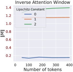
Figure 10: Spectral norm of pretrained $\mathbf{M}$ on $D(\operatorname{\mathcal{F}}_{L,\text{hills}})$ with three different choices of $L$ and varying $n$ along the $x$-axis.

We also demonstrate in Figure 10 that the attention window shrinks with increasing $n$ and $L$. Each point on the plot corresponds to an attention unit trained with tasks of a certain Lipschitzness using a varying number of tokens (depicted on the horizontal axis). The vertical axis depicts the norm $\|\mathbf{M}\|$ after training. We optimize using the Adam optimizer with a learning rate of $10^{-3}$. The attention units are pretrained and tested on $D(\operatorname{\mathcal{F}}_{L,\text{hills}})$. Each plot represents the ICL error after $1500$ iterations on tasks with varying Lipschitz constants as a function of the context length $n$. We set $d=2$, so $\{\operatorname{{\bf\it x}}_{i}\}$ can be parameterized by $\{\theta_{i}\}$ where $\theta_{i}$ denotes an angle from some fixed vector. $\{\theta_{i}\}$ are sampled uniformly from $[-\pi,\pi]$. The function class $D(\operatorname{\mathcal{F}}_{L,\text{hills}})$ which we use is defined above. We pretrain the attention unit over 1500 iterations, and repeat $3$ trials.

Figure 6. We randomly generate $\mathbf{B}$ on each trial by first sampling each element of $\hat{\mathbf{B}}$ i.i.d. from the standard normal distribution, then take its QR decomposition to obtain $\mathbf{B}.$ To draw the covariates, we draw a random matrix $\tilde{\mathbf{J}}\in\mathbb{R}^{d\times d}$ by sampling each element i.i.d. from the standard normal distribution. Then, we compute $\mathbf{J}=(\tilde{\mathbf{J}}^{\top}\tilde{\mathbf{J}})^{1/2}$. Then we draw $\tilde{\operatorname{{\bf\it x}}}_{i}\sim\mathcal{N}(\mathbf{0}_{d},\mathbf{I}_{d})$ and set $\operatorname{{\bf\it x}}_{i}=\frac{\mathbf{J}\tilde{\operatorname{{\bf\it x}}}_{i}}{\|\mathbf{J}\tilde{\operatorname{{\bf\it x}}}_{i}\|}$.

References

- Ahn et al. (2023) Ahn, K., Cheng, X., Daneshmand, H., and Sra, S. Transformers learn to implement preconditioned gradient descent for in-context learning, 2023.
- Akyürek et al. (2022) Akyürek, E., Schuurmans, D., Andreas, J., Ma, T., and Zhou, D. What learning algorithm is in-context learning? investigations with linear models. arXiv preprint arXiv:2211.15661, 2022.
- Bai et al. (2023) Bai, Y., Chen, F., Wang, H., Xiong, C., and Mei, S. Transformers as statisticians: Provable in-context learning with in-context algorithm selection, 2023.
- Bhattamishra et al. (2020) Bhattamishra, S., Ahuja, K., and Goyal, N. On the ability and limitations of transformers to recognize formal languages. arXiv preprint arXiv:2009.11264, 2020.
- Boix-Adsera et al. (2023) Boix-Adsera, E., Littwin, E., Abbe, E., Bengio, S., and Susskind, J. Transformers learn through gradual rank increase, 2023.
- Brown et al. (2020) Brown, T., Mann, B., Ryder, N., Subbiah, M., Kaplan, J. D., Dhariwal, P., Neelakantan, A., Shyam, P., Sastry, G., Askell, A., et al. Language models are few-shot learners. Advances in neural information processing systems, 33:1877–1901, 2020.
- Chen et al. (2023) Chen, Y., Tao, Q., Tonin, F., and Suykens, J. A. Primal-attention: Self-attention through asymmetric kernel svd in primal representation. arXiv preprint arXiv:2305.19798, 2023.
- Cheng et al. (2023) Cheng, X., Chen, Y., and Sra, S. Transformers implement functional gradient descent to learn non-linear functions in context. arXiv preprint arXiv:2312.06528, 2023.
- Chowdhery et al. (2023) Chowdhery, A., Narang, S., Devlin, J., Bosma, M., Mishra, G., Roberts, A., Barham, P., Chung, H. W., Sutton, C., Gehrmann, S., et al. Palm: Scaling language modeling with pathways. Journal of Machine Learning Research, 24(240):1–113, 2023.
- Dai et al. (2022) Dai, D., Sun, Y., Dong, L., Hao, Y., Sui, Z., and Wei, F. Why can gpt learn in-context? language models secretly perform gradient descent as meta optimizers. arXiv preprint arXiv:2212.10559, 2022.
- Deng et al. (2023a) Deng, Y., Li, Z., and Song, Z. Attention scheme inspired softmax regression, 2023a.
- Deng et al. (2023b) Deng, Y., Song, Z., and Zhou, T. Superiority of softmax: Unveiling the performance edge over linear attention. arXiv preprint arXiv:2310.11685, 2023b.
- Edelman et al. (2022) Edelman, B. L., Goel, S., Kakade, S., and Zhang, C. Inductive biases and variable creation in self-attention mechanisms. In International Conference on Machine Learning, pp. 5793–5831. PMLR, 2022.
- Fu et al. (2023a) Fu, D., Chen, T.-Q., Jia, R., and Sharan, V. Transformers learn higher-order optimization methods for in-context learning: A study with linear models. arXiv preprint arXiv:2310.17086, 2023a.
- Fu et al. (2023b) Fu, H., Guo, T., Bai, Y., and Mei, S. What can a single attention layer learn? a study through the random features lens. arXiv preprint arXiv:2307.11353, 2023b.
- Garg et al. (2022) Garg, S., Tsipras, D., Liang, P. S., and Valiant, G. What can transformers learn in-context? a case study of simple function classes. Advances in Neural Information Processing Systems, 35:30583–30598, 2022.
- Giannou et al. (2023) Giannou, A., Rajput, S., Sohn, J.-y., Lee, K., Lee, J. D., and Papailiopoulos, D. Looped transformers as programmable computers. arXiv preprint arXiv:2301.13196, 2023.
- Guo et al. (2023) Guo, T., Hu, W., Mei, S., Wang, H., Xiong, C., Savarese, S., and Bai, Y. How do transformers learn in-context beyond simple functions? a case study on learning with representations. arXiv preprint arXiv:2310.10616, 2023.
- Han et al. (2023) Han, C., Wang, Z., Zhao, H., and Ji, H. In-context learning of large language models explained as kernel regression. arXiv preprint arXiv:2305.12766, 2023.
- Han et al. (2022) Han, X., Ren, T., Nguyen, T. M., Nguyen, K., Ghosh, J., and Ho, N. Designing robust transformers using robust kernel density estimation. arXiv preprint arXiv:2210.05794, 2022.
- Hardy et al. (1952) Hardy, G., Littlewood, J., and Pólya, G. Inequalities. Cambridge Mathematical Library. Cambridge University Press, 1952. ISBN 9780521358804. URL https://books.google.com/books?id=t1RCSP8YKt8C.
- Huang et al. (2023) Huang, Y., Cheng, Y., and Liang, Y. In-context convergence of transformers. arXiv preprint arXiv:2310.05249, 2023.
- Jelassi et al. (2022) Jelassi, S., Sander, M. E., and Li, Y. Vision transformers provably learn spatial structure, 2022.
- Kim et al. (2020) Kim, H., Papamakarios, G., and Mnih, A. The lipschitz constant of self-attention, 2020.
- Knaeble (2015) Knaeble, B. Variations on the projective central limit theorem. https://arxiv.org/pdf/0904.1048.pdf, 2015.
- Li et al. (2023a) Li, H., Wang, M., Liu, S., and Chen, P.-Y. A theoretical understanding of shallow vision transformers: Learning, generalization, and sample complexity. arXiv preprint arXiv:2302.06015, 2023a.
- Li et al. (2023b) Li, Y., Ildiz, M. E., Papailiopoulos, D., and Oymak, S. Transformers as algorithms: Generalization and stability in in-context learning. In International Conference on Machine Learning, pp. 19565–19594. PMLR, 2023b.
- Li et al. (2023c) Li, Y., Li, Y., and Risteski, A. How do transformers learn topic structure: Towards a mechanistic understanding. arXiv preprint arXiv:2303.04245, 2023c.
- Lieb & Loss (2001) Lieb, E. H. and Loss, M. Analysis, volume 14. American Mathematical Soc., 2001.
- Likhosherstov et al. (2021) Likhosherstov, V., Choromanski, K., and Weller, A. On the expressive power of self-attention matrices. arXiv preprint arXiv:2106.03764, 2021.
- Lin et al. (2023) Lin, L., Bai, Y., and Mei, S. Transformers as decision makers: Provable in-context reinforcement learning via supervised pretraining. arXiv preprint arXiv:2310.08566, 2023.
- Liu et al. (2022) Liu, B., Ash, J. T., Goel, S., Krishnamurthy, A., and Zhang, C. Transformers learn shortcuts to automata. arXiv preprint arXiv:2210.10749, 2022.
- Mahankali et al. (2023) Mahankali, A., Hashimoto, T. B., and Ma, T. One step of gradient descent is provably the optimal in-context learner with one layer of linear self-attention. arXiv preprint arXiv:2307.03576, 2023.
- Min et al. (2022) Min, S., Lewis, M., Zettlemoyer, L., and Hajishirzi, H. Metaicl: Learning to learn in context. In Proceedings of the 2022 Conference of the North American Chapter of the Association for Computational Linguistics: Human Language Technologies. Association for Computational Linguistics, 2022. doi: 10.18653/v1/2022.naacl-main.201. URL http://dx.doi.org/10.18653/v1/2022.naacl-main.201.
- Nguyen et al. (2022) Nguyen, T., Pham, M., Nguyen, T., Nguyen, K., Osher, S., and Ho, N. Fourierformer: Transformer meets generalized fourier integral theorem. Advances in Neural Information Processing Systems, 35:29319–29335, 2022.
- Olsson et al. (2022) Olsson, C., Elhage, N., Nanda, N., Joseph, N., DasSarma, N., Henighan, T., Mann, B., Askell, A., Bai, Y., Chen, A., et al. In-context learning and induction heads. arXiv preprint arXiv:2209.11895, 2022.
- Pérez et al. (2021) Pérez, J., Barceló, P., and Marinkovic, J. Attention is turing complete. The Journal of Machine Learning Research, 22(1):3463–3497, 2021.
- Rae et al. (2021) Rae, J. W., Borgeaud, S., Cai, T., Millican, K., Hoffmann, J., Song, F., Aslanides, J., Henderson, S., Ring, R., Young, S., et al. Scaling language models: Methods, analysis & insights from training gopher. arXiv preprint arXiv:2112.11446, 2021.
- Raventós et al. (2023) Raventós, A., Paul, M., Chen, F., and Ganguli, S. Pretraining task diversity and the emergence of non-bayesian in-context learning for regression. arXiv preprint arXiv:2306.15063, 2023.
- Robbins (1955) Robbins, H. A remark on stirling’s formula. The American Mathematical Monthly, 62(1):26–29, 1955. ISSN 00029890, 19300972. URL http://www.jstor.org/stable/2308012.
- Sanford et al. (2023) Sanford, C., Hsu, D., and Telgarsky, M. Representational strengths and limitations of transformers. arXiv preprint arXiv:2306.02896, 2023.
- Shen et al. (2023) Shen, L., Mishra, A., and Khashabi, D. Do pretrained transformers really learn in-context by gradient descent? arXiv preprint arXiv:2310.08540, 2023.
- Shi et al. (2022) Shi, Z., Wei, J., and Liang, Y. A theoretical analysis on feature learning in neural networks: Emergence from inputs and advantage over fixed features. arXiv preprint arXiv:2206.01717, 2022.
- Song et al. (2023) Song, Z., Xu, G., and Yin, J. The expressibility of polynomial based attention scheme, 2023.
- Tarzanagh et al. (2023a) Tarzanagh, D. A., Li, Y., Thrampoulidis, C., and Oymak, S. Transformers as support vector machines. arXiv preprint arXiv:2308.16898, 2023a.
- Tarzanagh et al. (2023b) Tarzanagh, D. A., Li, Y., Zhang, X., and Oymak, S. Max-margin token selection in attention mechanism, 2023b.
- Thoppilan et al. (2022) Thoppilan, R., De Freitas, D., Hall, J., Shazeer, N., Kulshreshtha, A., Cheng, H.-T., Jin, A., Bos, T., Baker, L., Du, Y., et al. Lamda: Language models for dialog applications. arXiv preprint arXiv:2201.08239, 2022.
- Tian et al. (2023) Tian, Y., Wang, Y., Zhang, Z., Chen, B., and Du, S. Joma: Demystifying multilayer transformers via joint dynamics of mlp and attention. arXiv preprint arXiv:2310.00535, 2023.
- Trockman & Kolter (2023) Trockman, A. and Kolter, J. Z. Mimetic initialization of self-attention layers, 2023.
- Tsai et al. (2019) Tsai, Y.-H. H., Bai, S., Yamada, M., Morency, L.-P., and Salakhutdinov, R. Transformer dissection: a unified understanding of transformer’s attention via the lens of kernel. arXiv preprint arXiv:1908.11775, 2019.
- Vaswani et al. (2017) Vaswani, A., Shazeer, N., Parmar, N., Uszkoreit, J., Jones, L., Gomez, A. N., Kaiser, Ł., and Polosukhin, I. Attention is all you need. Advances in neural information processing systems, 30, 2017.
- von Oswald et al. (2023a) von Oswald, J., Niklasson, E., Randazzo, E., Sacramento, J., Mordvintsev, A., Zhmoginov, A., and Vladymyrov, M. Transformers learn in-context by gradient descent. In International Conference on Machine Learning, pp. 35151–35174. PMLR, 2023a.
- von Oswald et al. (2023b) von Oswald, J., Niklasson, E., Schlegel, M., Kobayashi, S., Zucchet, N., Scherrer, N., Miller, N., Sandler, M., Vladymyrov, M., Pascanu, R., et al. Uncovering mesa-optimization algorithms in transformers. arXiv preprint arXiv:2309.05858, 2023b.
- Vuckovic et al. (2020) Vuckovic, J., Baratin, A., and des Combes, R. T. A mathematical theory of attention, 2020.
- Wang et al. (2023) Wang, X., Zhu, W., and Wang, W. Y. Large language models are implicitly topic models: Explaining and finding good demonstrations for in-context learning. arXiv preprint arXiv:2301.11916, 2023.
- Wei et al. (2022) Wei, C., Chen, Y., and Ma, T. Statistically meaningful approximation: a case study on approximating turing machines with transformers. Advances in Neural Information Processing Systems, 35:12071–12083, 2022.
- Wen & Li (2021) Wen, Z. and Li, Y. Toward understanding the feature learning process of self-supervised contrastive learning. In International Conference on Machine Learning, pp. 11112–11122. PMLR, 2021.
- Wibisono & Wang (2023) Wibisono, K. C. and Wang, Y. On the role of unstructured training data in transformers’ in-context learning capabilities. In NeurIPS 2023 Workshop on Mathematics of Modern Machine Learning, 2023.
- Wu et al. (2023) Wu, J., Zou, D., Chen, Z., Braverman, V., Gu, Q., and Bartlett, P. L. How many pretraining tasks are needed for in-context learning of linear regression? arXiv preprint arXiv:2310.08391, 2023.
- Xie et al. (2021) Xie, S. M., Raghunathan, A., Liang, P., and Ma, T. An explanation of in-context learning as implicit bayesian inference. arXiv preprint arXiv:2111.02080, 2021.
- Yun et al. (2019) Yun, C., Bhojanapalli, S., Rawat, A. S., Reddi, S. J., and Kumar, S. Are transformers universal approximators of sequence-to-sequence functions? arXiv preprint arXiv:1912.10077, 2019.
- Zhang et al. (2023) Zhang, R., Frei, S., and Bartlett, P. L. Trained transformers learn linear models in-context. arXiv preprint arXiv:2306.09927, 2023.