Abstract

We investigate wormhole solutions using the modified gravity model $f(Q,T)$ with viscosity and aim to find a solution for the existence of wormholes mathematically without violating the energy conditions. We show that there is no need to define a wormhole from exotic matter and analyze the equations with numerical analysis to establish weak energy conditions. In the numerical analysis, we found that the appropriate values of the parameters can maintain the weak energy conditions without the need for exotic matter. Adjusting the parameters of the model can increase or decrease the rate of positive energy density or radial and tangential pressures. According to the numerical analysis conducted in this paper, the weak energy conditions are established in the whole space if $\alpha<0$, $12.56<\beta<25.12$ or $\alpha>0$, $\beta>25.12$. The analysis also showed that the supporting matter of the wormhole is near normal matter, indicating that the generalized $f(Q,T)$ model with viscosity has an acceptable parameter space to describe a wormhole without the need for exotic matter.

PACS:  95.36.+x, 98.80.-k, 04.50.kd
Key Words: Wormhole, $f(Q,T)$ Gravity, Black Hole.

1 Introduction

A wormhole is a theoretical concept in physics that suggests the existence of a shortcut or tunnel between two distant points in space or time (Kanti et al, 2012; Lin et al., 2019; Parsaei et al., 2020; Wang, 2022). It is often depicted as a tunnel that connects two separate regions of the universe, allowing for faster travel or even time travel. According to Einstein’s theory of general relativity, certain solutions of the equations allow for the existence of wormholes. However, creating a traversable wormhole would require exotic matter with negative energy density and large negative pressure (Anchordoqui et al, 1997). This type of matter has not been observed in nature so far. It is important to note that wormholes are still purely theoretical and have not been proven to exist. Scientists continue to study and explore the possibilities of wormholes within the framework of theoretical physics (Kanti et al, 2012; Anchordoqui et al, 1997; Richarte et al, 2008; Lobo et al, 2009; Moraes et al, 2017a; Moraes et al, 2017b, Lin et al., 2019; Parsaei et al., 2020; Wang, 2022). In 1935, Einstein and physicist Nathan Rosen proposed the existence of ”bridges” or ”wormholes” that could connect two separate points in space-time (Kanti et al, 2012). These theoretical structures would require the presence of exotic matter with negative energy density and negative pressure to keep the wormhole stable and traversable. It is worth noting that traversable wormholes, which would allow objects or information to pass through them would require the presence of exotic matter with properties that are not currently known to exist in nature (Lobo et al, 2009). Additionally, wormholes are subject to various theoretical challenges, such as the potential for instability, high radiation, and the need for advanced technology to create and sustain them (Lobo et al, 2009; Moraes et al, 2017a; Moraes et al, 2017b). Researchers continue to study the theoretical properties and implications of wormholes within the framework of general relativity and quantum physics, but more research is needed to determine if they can exist in reality (Moraes et al, 2017a; Moraes et al, 2017b; Parsaei et al., 2020; Wang, 2022).
Black Holes and Wormholes are distinct concepts in the field of astrophysics and general relativity. While they share certain similarities, such as their association with extreme gravity, they have fundamental differences: A Black Hole is a cosmic object formed from the collapse of massive stars or through other astrophysical processes. It has an event horizon, a boundary beyond which nothing, not even light, can escape the gravitational pull of the Black Hole. The collapsed matter at the center of a Black Hole is known as a singularity, where the laws of physics, as we currently understand them, break down. Black Holes are characterized by their mass, spin (angular momentum), and electric charge. They are observed as regions in space with exceptionally strong gravitational effects, often accompanied by the accretion of matter from surrounding sources (Jamil et al, 2012; Gadbail et al., 2021). On the other hand, a wormhole is a speculative concept in theoretical physics that suggests the existence of a shortcut or passage between two different regions of space-time. It is often depicted as a tunnel-like structure connecting two distant points in the universe. The stability of wormholes is a major challenge, as they are prone to collapse or require precise arrangements of matter to maintain their integrity. While Black Holes and Wormholes are distinct concepts, there is a historical connection between them (Elizalde et al, 2019). Further scientific research is needed to explore the properties and potential existence of wormholes in the universe.
$f(Q)$ gravity is a modified theory of gravity that extends the symmetric teleparallel equivalent of General Relativity (GR) (Cai et al, 2016). In $f(Q)$ gravity, the gravitational interaction is driven by a nonmetricity scalar called $Q$. This theory has gained attention in the field of cosmology due to its potential to explain various phenomena, such as dark energy and the accelerated expansion of the universe (Cai et al, 2016; Jimeneza et al, 2019; Jimenez et al, 2018; Paliathanasis, 2023). Cosmological models based on $f(Q)$ gravity have shown efficiency in fitting observational data sets at both the background and perturbation levels (Cai et al, 2016; Jimeneza et al, 2019). Also, $f(Q)$ gravity provides a complete dark energy scenario, where the nonmetricity scalar $Q$ describes the gravitational interaction (Jimeneza et al, 2019; Jimenez et al, 2018; Solanki et al., 2021). We know that the $\Lambda CDM$ Universe can be reconstructed in terms of e-folding in $f(Q)$ gravity (Paliathanasis, 2023). Some models have been studied in $f(Q)$ gravity to understand its implications and compare them with observational data (Xu et al, 2019; Paliathanasis, 2023; Shabani et al, 2023; Calza et al, 2023; Albuquerque et al, 2022). Also, the evolution of linear perturbations in $f(Q)$ gravity has been investigated, with the design of $f(Q)$ to achieve specific cosmological implications (Xu et al, 2019; Albuquerque et al, 2022; Calza et al, 2023). Energy conditions have been explored in $f(Q)$ gravity, which falls under the class of teleparallel theories of gravity (Cai et al, 2016). On the other hand, an extension of $f(Q)$ gravity is $f(Q,T)$ gravity (we use this model in the following), where $T$ represents the trace of the energy-momentum tensor. This extension introduces an extra force on massive particles due to the coupling between $Q$ and $T$ (Xu et al, 2019). Following, the $f(Q,T)$ modified gravity model with viscosity is chosen for investigating wormholes due to its ability to provide alternative explanations to standard gravity, and its cosmological consequences. Therefore, it distinguishes it from other modified gravity models that may have different modifications or additional parameters. Also, bulk viscosity is the only viscous influence that can change the background dynamics in a homogeneous and isotropic(anisotropic) universe (confirmed by recent observational data). The role of viscosity is in understanding the accelerated expansion of the universe and its implications for wormholes. Besides, the $f(Q,T)$ modified gravity model with viscosity is used to investigate the properties and behavior of wormholes, such as their stability, formation, and potential traversability.
Therefore, according to the above discussions, we organized the structures of this work as follows: in Section 2, we consider a modified $f(Q,T)$ gravity model with viscosity contain and numerically investigates the wormhole solution in some special functions. Finally, in Section 3, the conclusion and summary are offered.

2 Wormhole Solution in $f(Q,T)$ Gravity Model

Einstein’s theory of general relativity allows for the existence of wormholes as a theoretical possibility, their actual existence in the universe remains hypothetical. Modified gravity models, on the other hand, introduce modifications to Einstein’s theory of general relativity to address certain unresolved issues or to incorporate additional phenomena. These modifications can lead to different predictions for the behavior and properties of wormholes compared to those derived from general relativity. It is important to note that the predictions of modified gravity models for wormholes can vary depending on the specific modifications introduced and the assumptions made in those models. Some modified gravity models may propose alternative explanations for wormholes or suggest different properties and behaviors for these hypothetical structures. Altogether, both Einstein’s theory of general relativity and modified gravity models allow for the possibility of wormholes, but their predictions and implications can differ. There are both discrepancies and points of convergence when comparing the predictions for wormholes in modified gravity models with those derived from Einstein’s theory of general relativity or other established models. 1)Discrepancies: Modified gravity models introduce modifications to general relativity, which can lead to different predictions for the behavior and properties of wormholes compared to those derived from general relativity. Wormholes in modified gravity models may not require exotic matter to prevent collapse, unlike in general relativity. 2)Points of Convergence: Both general relativity and modified gravity models allow for the possibility of wormholes as theoretical constructs. Wormholes are solutions to the Einstein field equations for gravity, which are the foundation of general relativity (Lin et al., 2019; Parsaei et al., 2020; Wang, 2022).
One of the fascinating aspects of $f(Q,T)$ gravity is its potential to provide solutions for the existence of wormholes without the need for exotic matter. In the following, the goal is to find solutions that do not violate energy conditions and are consistent with the laws of physics.

2.1 Generalized Gravity Model $f(Q,T)$

To better understand the nature of wormholes and their theoretical underpinnings, we have explored modified theories of gravity. One such theory is $f(Q,T)$ gravity, an extension of the symmetric teleparallel equivalent of General Relativity (Cai et al, 2016). In $f(Q,T)$ gravity, the gravitational interaction is driven by a nonmetricity scalar called $Q$, which offers potential explanations for phenomena like dark energy and the accelerated expansion of the universe [Cai et al, 2016; Jimeneza et al, 2019; Xu et al, 2019). By generalizing the gravity model $f(Q)$, we can get the gravity model $f(Q,T)$, the action of this model is expressed as follows (Jimeneza et al, 2019)

$$S=\int d^{4}x(\frac{1}{16\pi}f(Q,T)+L_{m})\sqrt{-g}$$ (1)

where $Q$ is the nonmetricity parameter, $T$ is the trace energy-momentum tensor, $L_{m}$ stands for the matter Lagrangian and $g=det(g_{\mu\nu})$. If we take the derivative of this action with respect to the metric and connection, the equations of motion are obtained as follows

$$-\frac{2}{\sqrt{-g}}\nabla_{\lambda}(\sqrt{-g}f_{Q}P^{\lambda}{}_{\mu\nu})-\frac{1}{2}fg_{\mu\nu}+f_{T}(T_{\mu\nu}+\theta_{\mu\nu})-f_{Q}(P_{\nu\rho\sigma}Q_{\mu}{}^{\rho\sigma}-2P_{\rho\sigma\mu}Q^{\rho\sigma}{}_{\nu})=8\pi T_{\mu\nu}$$

$$\nabla_{\mu}\nabla_{\nu}(\sqrt{-g}f_{Q}P_{\alpha}^{\mu\nu}+4\pi H_{\alpha}^{\mu\nu})=0$$ (2)

where $f_{T}=\frac{\partial f}{\partial T}$, non-metricity tensor $Q_{\lambda\mu\nu}=\nabla_{\lambda}g_{\mu\nu}$, $P^{\lambda}_{\mu\nu}$ is the superpotential, $f_{Q}=\frac{\partial f}{\partial Q}$, and $H_{\alpha}^{\mu\nu}$ is the density of the hypermomentum and are defined as follows (Jimeneza et al, 2019)

$$H_{\lambda}^{\mu\nu}\equiv\frac{\sqrt{-g}}{16\pi}f_{T}\frac{\delta T}{\delta\hat{\Gamma}_{\mu\nu}^{\lambda}}+\frac{\delta\sqrt{-g}L_{M}}{\delta\hat{\Gamma}_{\mu\nu}^{\lambda}}$$ (3)

where $\hat{\Gamma}_{\mu\nu}^{\lambda}$ is the Levi-Civita connection. To calculate $f_{T}(T_{\mu\nu}+\theta_{\mu\nu})$ that appeared in the equations of motion, we need to specify the tensors $T_{\mu\nu},\theta_{\mu\nu}$ in the model. The momentum energy tensor and $\theta_{\mu\nu}$ tensor are defined as follows

$$T_{\mu\nu}\equiv-\frac{2}{\sqrt{-g}}\frac{\delta(\sqrt{-g}L_{M})}{\delta g^{\mu\nu}}$$ (4)

$$\theta_{\mu\nu}=g^{\alpha\beta}\frac{\delta T_{\alpha\beta}}{\delta g^{\mu\nu}}.$$ (5)

2.2 Wormhole Solution in $f(Q,T)$ Model with Viscosity

It is worth mentioning that wormhole physics is a subject of ongoing research and exploration within the field of theoretical physics. Wormholes are solutions derived from the field equations in Einstein’s theory of gravitation, and their mathematical description involves concepts from general relativity and differential geometry. However, wormhole solutions have been studied using various mathematical approaches and techniques. Some studies have explored wormholes with variable equations of state (EoS) parameters, where the violation of energy conditions is minimized or controlled (that we use in our paper). We explored wormholes with variable equations of state (EoS) parameters, where the ratio of pressure to energy density $(\omega=\frac{p}{\rho})$ is a function of the radial/tangential coordinate and we found a specific situation where the energy conditions are satisfied. Other researchers have used the cut-and-paste method to find wormhole solutions of finite size that minimize the violation of energy conditions (Solanki et al., 2021). In summary, wormholes are solutions derived from the field equations in Einstein’s theory of gravitation, and their mathematical description involves concepts from general relativity and differential geometry.
To calculate the solution of the wormhole, we assume the metric to be static and have spherical symmetry. Using the Schwarzschild coordinates $(t,r,\varphi,\theta)$, we have

$$ds^{2}=(e^{2\phi(r)})dt^{2}-(1-\frac{b(r)}{r})^{-1}dr^{2}-(r^{2})d\theta^{2}-(r^{2}\sin^{2}\theta)d\varphi^{2}$$ (6)

where $b(r),\phi(r)$ are shape function and redshift function respectively. We know that wormhole solution in any gravity model should apply in the following conditions (Jamil et al, 2012; Kanti et al, 2012; Anchordoqui et al, 1997; Richarte et al, 2008; Lobo et al, 2009; Moraes et al, 2017a; Moraes et al, 2017b):
1) In the state $r>r_{0}$, shape function should be to form $b(r)<r$, But in the throat of the wormhole $r=r_{0}$, it must be $b(r_{0})=r_{0}$.
2) The shape function must satisfy the flaring out, this means $b^{\prime}(r_{0})<1$.
3) We need the condition of being asymptotically flat when $r\to\infty$ then $\frac{b(r)}{r}\to 1$
4) The redshift function $\phi(r)$ must be bounded at all points in space.
Due to the pressure difference in the tangential and radial direction, the condition of anisotropy is established, so the momentum energy tensor is expressed as follows

$$T_{\mu}^{\nu}=(\rho+P_{t})U_{\mu}U^{\nu}-P_{t}\delta_{\mu}^{\nu}-(P_{r}-P_{t})V_{\mu}V^{\nu}$$ (7)

where $\rho,P_{r},P_{t}$ are the density of the universe, the radial pressure and the tangential pressure and are a function of radial coordinate $r$. $U_{\mu}$ and $V_{\mu}$ are the four-velocity vector and unitary space-like vectors. Also, the trace of the momentum energy tensor will be $T=\rho-P_{r}-2P_{t}$. If we consider the Lagrangian of the matter according to (Richarte et al, 2008; Lobo et al, 2009; Moraes et al, 2017a; Moraes et al, 2017b; Jamil et al, 2012) to be equal to $L_{m}=P$, the equation (5) becomes as follows

$$\theta_{\mu\nu}=-g_{\mu\nu}P-2T_{\mu\nu}$$ (8)

where $P=\frac{P_{r}+2P_{t}}{3}$. The nonmetricity according to the spherically symmetric metric is as follows

$$Q=\frac{-b}{r^{2}}[\frac{rb^{\prime}-b}{r(r-b)}+2\phi^{\prime}]$$ (9)

Now we can calculate the equations of motion by using the metric and tensor of momentum energy and the tensor of nonmetricity. Therfore, by using equations (9), (7) and (6) ,and inserting them in the equation of motion (2), we have

$$8\pi\rho=\left(\frac{r-b}{2r^{3}}\right)[f_{Q}\left(\frac{\left(2r-b\right)\left(rb^{\prime}-b\right)}{\left(r-b\right)^{2}}+\frac{\left(2+2r\phi^{\prime}\right)b}{r-b}\right)$$

$$+f_{QQ}Q^{\prime}\left(2\frac{br}{r-b}\right)+f\left(\frac{r^{3}}{r-b}\right)+f_{T}\left(\frac{2r^{3}}{r-b}\right)\left(P+\rho\right)]$$ (10)

$$8\pi P_{r}=-\left(\frac{r-b}{2r^{3}}\right)[f_{Q}\left(\frac{b}{r-b}\left(\frac{\left(rb^{\prime}-b\right)}{r-b}+2+2r\phi^{\prime}\right)-4r\phi^{\prime}\right)$$

$$+\frac{2br}{r-b}f_{QQ}Q^{\prime}+f\left(\frac{r^{3}}{r-b}\right)-2\left(\frac{r^{3}}{r-b}\right)f_{T}\left(P-P_{r}\right)]$$ (11)

$$8\pi P_{t}=-\left(\frac{r-b}{4r^{2}}\right)[f_{Q}\left(\frac{\left(rb^{\prime}-b\right)\left(\frac{2r}{r-b}+2r\phi^{\prime}\right)}{r\left(r-b\right)}+\frac{4\left(2b-r\right)\left(\phi^{\prime}\right)}{\left(r-b\right)}-4r\left(\phi^{\prime}\right)^{2}-4r\phi^{\prime\prime}\right)$$

$$-4rf_{QQ}Q^{\prime}\phi^{\prime}+\frac{2fr^{2}}{r-b}-\frac{4r^{2}f_{T}\left(P-P_{t}\right)}{r-b}]$$ (12)

where prime denotes derivative to $r$. To solve the equations of motion, the function $f(Q,T)$ of the model must be known. According to (Xu et al, 2019), we consider the gravitational function $f(Q,T)$ of our model as $f(Q,T)=\alpha Q^{-1}+\beta T$ ($\alpha$ and $\beta$ are arbitrary parameters). Also, we choose shape and redsift functions as (Tayde et al., 2023)

$$b(r)=r_{0}(\frac{r_{0}}{r})^{n}$$ (13)

$$\phi(r)=\phi_{0}(\frac{r_{0}}{r})^{m}$$ (14)

where $r_{0}$ is a positive constant and $\phi_{0}$ is an arbitrary constant value and $n$,$m$ are constant exponents which are strictly positive to satisfy the asymptotic flatness condition (Tayde et al., 2023). Therefore, with these functions, we will have three equations of motion and three unknown cosmic parameters that we can solve.
But one of our assumptions in this article is the presence of viscosity in the universe, so the pressure in the radial and tangential direction is obtained according to the following equations (Wang, 2022; Parsaei et al, 2022)

$$P_{r}{}_{v}=P_{r}-3\xi H_{0}$$ (15)

$$P_{t}{}_{v}=P_{t}-3\xi H_{0}$$ (16)

which $\xi$ (viscosity parameter) is defined as follows

$$\xi=\xi_{0}+\xi_{1}H_{0}$$ (17)

where $H_{0}=73.24\,kms^{-1}Mpc^{-1}$ and $\xi_{0}\simeq 10^{-6}$ (Wang, 2022), for simplicity we consider $\xi_{1}=0$ (Here we used a similar procedure in (Wang, 2022) to introduce the viscosity effect $-3\xi H_{0}$ in the equations). Now by using above equations in and the equations (11) and (12), the field equations for tangential and radial pressure in the case that the wormhole has viscosity will be as follows

$$8\pi P_{rv}=-\left(\frac{r-b}{2r^{3}}\right)[f_{Q}\left(\frac{b}{r-b}\left(\frac{\left(rb^{\prime}-b\right)}{r-b}+2+2r\phi^{\prime}\right)-4r\phi^{\prime}\right)$$

$$+\frac{2br}{r-b}f_{QQ}Q^{\prime}+f\left(\frac{r^{3}}{r-b}\right)-2\left(\frac{r^{3}}{r-b}\right)f_{T}\left(P-P_{r}\right)]$$ (18)

$$8\pi P_{tv}=-\left(\frac{r-b}{4r^{2}}\right)[f_{Q}\left(\frac{\left(rb^{\prime}-b\right)\left(\frac{2r}{r-b}+2r\phi^{\prime}\right)}{r\left(r-b\right)}+\frac{4\left(2b-r\right)\left(\phi^{\prime}\right)}{\left(r-b\right)}-4r\left(\phi^{\prime}\right)^{2}-4r\phi^{\prime\prime}\right)$$

$$-4rf_{QQ}Q^{\prime}\phi^{\prime}+\frac{2fr^{2}}{r-b}-\frac{4r^{2}f_{T}\left(P-P_{t}\right)}{r-b}]$$ (19)

For the simplicity of calculations, we simplify equations and ignore powers higher than $r^{3}$. Therefore, we have

$$\rho=\frac{r^{3}\alpha\beta{{\phi}_{0}}^{2}}{24{r_{0}}(32{\pi}^{2}-12\pi\beta+{\beta}^{2})}$$ (20)

$$P_{rv}=-\frac{5\pi r^{3}\alpha\beta{{\phi}_{0}}^{2}}{3{r_{0}}(4\pi-\beta)(8\pi-\beta)(8\pi+\beta)}+\frac{7r^{3}\alpha{\beta}^{2}{{\phi}_{0}}^{2}}{24{r_{0}}(4\pi-\beta)(8\pi-\beta)(8\pi+\beta)}$$ (21)

$$P_{tv}=-\frac{8{\pi}^{2}r^{3}\alpha{{\phi}_{0}}^{2}}{{r_{0}}(8\pi+\beta)(32{\pi}^{2}-12\pi\beta+{\beta}^{2})}+\frac{4\pi r^{3}\alpha\beta{{\phi}_{0}}^{2}}{3{r_{0}}(8\pi+\beta)(32{\pi}^{2}-12\pi\beta+{\beta}^{2})}+\frac{r^{3}\alpha{\beta}^{2}{{\phi}_{0}}^{2}}{24{r_{0}}(8\pi+\beta)(32{\pi}^{2}-12\pi\beta+{\beta}^{2})}$$ (22)

Now, we can check the condition of weak energy for the existence of wormhole solution despite the presence of viscosity. According to the condition of weak energy, the following three conditions should be satisfied

$$\rho\geq 0\,\,\,\,,\,\,\,\rho+P_{rv}\geq 0\,\,\,,\,\,\,\rho+P_{tv}\geq 0\,$$ (23)

Also, we should check the border equation $r_{0}$ in the wormhole throat. According to the boundary condition $r=r_{0}$, we have

$$\rho+P_{tv}=-\frac{{{r_{0}}}^{2}\alpha(24\pi+\beta){{\phi}_{0}}^{2}}{768{\pi}^{2}-12{\beta}^{2}}$$ (24)

$$\rho+P_{rv}=-\frac{{{r_{0}}}^{2}\alpha\beta{{\phi}_{0}}^{2}}{192{\pi}^{2}-3{\beta}^{2}}$$ (25)

For checking the condition of weak energy (23), we have the following equations

$$\rho=\frac{r^{3}\alpha\beta{{\phi}_{0}}^{2}}{24{r_{0}}(32{\pi}^{2}-12\pi\beta+{\beta}^{2})}\geq 0$$ (26)

$$\rho+P_{tv}=-\frac{r^{3}\alpha(24\pi+\beta){{\phi}_{0}}^{2}}{12{r_{0}}(8\pi-\beta)(8\pi+\beta)}\geq 0$$ (27)

$$\rho+P_{rv}=-\frac{r^{3}\alpha\beta{{\phi}_{0}}^{2}}{192{\pi}^{2}{r_{0}}-3{r_{0}}{\beta}^{2}}\geq 0$$ (28)

By determining the sign of equations (26,27,28), we obtain the allowed intervals for the values $\alpha$ and $\beta$ so that the boundary condition and the weak energy condition are established. In this regard, we have

$$\alpha<0\,\,\,,\,\,\,4\pi<\beta<8\pi$$ (29)

$$\alpha>0\,\,\,,\,\,\,\beta>8\pi\,$$ (30)

Using equations (20,21,22) and according to the equation of state $\rho=\frac{P}{\omega}=(\frac{P_{rv}+2P_{tv}}{3\omega})$, we have

$$\rho=-\frac{r^{3}\alpha(16\pi-3\beta){\phi_{0}}^{2}}{24r_{0}\omega(32{\pi}^{2}-12\pi\beta+{\beta}^{2})}$$ (31)

$$\rho+P_{tv}=-\frac{r^{3}\alpha(64{\pi}^{2}(2+3\omega)-(3+\omega){\beta}^{2}-8\pi(\beta+4\omega\beta)){\phi_{0}}^{2}}{24r_{0}}\omega(8\pi+\beta)(32{\pi}^{2}-12\pi\beta+{\beta}^{2})$$ (32)

$$\rho+P_{rv}=-\frac{r^{3}\alpha(128{\pi}^{2}+8\pi(-1+5\omega)\beta-(3+7\omega){\beta}^{2}){\phi_{0}}^{2}}{24r_{0}}\omega(4\pi-\beta)(8\pi-\beta)(8\pi+\beta)$$ (33)

Now, using these equations, we can check the different behaviors of the wormhole according to the different $\omega$ values. To further understand the conditions for establishing traversable wormholes, we have employed numerical analysis techniques. By analyzing the equations in $f(Q,T)$ gravity model, we determine and study the implications of weak energy conditions. These investigations offer valuable insights into the potential existence and properties of wormholes within the framework of $f(Q,T)$ gravity.

2.3 Numerical Analysis of Equations

Energy conditions are important in studying the properties of spacetime and the matter sources that generate it. For example, the violation of the NEC in a wormhole solution would indicate the presence of exotic matter in the throat of the wormhole. Additionally, a positive energy density is required for a physically realistic matter source that can sustain a wormhole solution in general relativity.

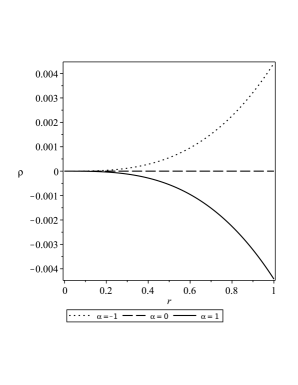
Figure 1: Plot of parameter $\rho$ (eV) versus $r$ (m) for $r_{0}=2,\phi_{0}=-1$ , $\beta=15,\omega=-1$ and $\alpha=-1,0,1$ (we use units $\hbar=c=1$ in our calculations and some parameters are dimensionless).

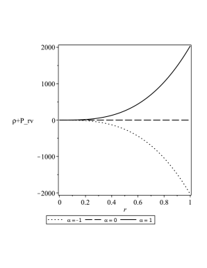
Figure 2: Plot of parameter ($\rho+P_{rv}$) versus $r$ (m) for $r_{0}=2,\phi_{0}=-1$ , $\beta=15,\omega=-1$ and $\alpha=-1,0,1$.

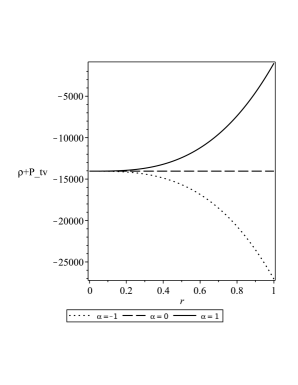
Figure 3: Plot of parameter ($\rho+P_{tv}$) versus $r$ (m) for $r_{0}=2,\phi_{0}=-1$ , $\beta=15,\omega=-1$ and $\alpha=-1,0,1$.

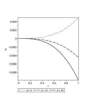
Figure 4: Plot of parameter ($\rho$) versus $r$ (m) for $r_{0}=2,\phi_{0}=-1$ , $\alpha=1,\omega=-1$ and $\beta=5,15,30$.

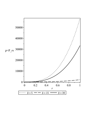
Figure 5: Plot of parameter ($\rho+P_{rv}$) versus $r$ (m) for $r_{0}=2,\phi_{0}=-1$ , $\alpha=1,\omega=-1$ and $\beta=5,15,30$.

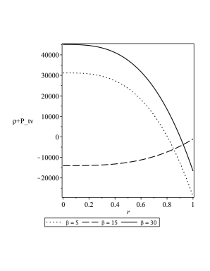
Figure 6: Plot of parameter ($\rho+P_{tv}$) versus $r$ (m) for $r_{0}=2,\phi_{0}=-1$ , $\alpha=1,\omega=-1$ and $\beta=5,15,30$.

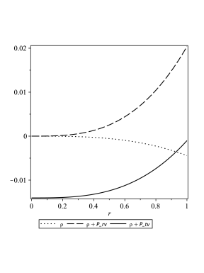
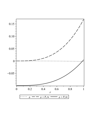
Figure 7: Variation of parameters ($\rho,P_{rv},P_{tv}$) relative to $r$ (m) with $\omega=-1$ (left), $\omega=-2$ (right) for $r_{0}=2,\phi_{0}=-1,\alpha=1,\beta=15$. *we have rescaled the graphs for better interpretation*

In the following, we check the weak energy conditions using the field equations. Based on this, in figures (1-7), the graphs of $\rho+P_{rv},\rho+P_{tv},\rho$ have been drawn in terms of $r$, where we have assumed $r_{0}=2,\phi_{0}=-1$. We know that due to the positiveness of $\rho$ and $\rho+P_{r}$, weak energy conditions are established in the whole space, and if $\rho$ is negative, the weak energy conditions are violated in the whole space. Therefore, according figures (1-7), we showed that based on the appropriate values of the parameters, weak energy condition is maintained if $\alpha<0~{},~{}12.56<\beta<25.12$ or $\alpha>0~{},~{}\beta>25.12$. On the other hand, the adjustment of some parameters is necessary to increase or decrease the rate of positive energy density or radial and tangential pressures. Also, according to the figure (7), it is clear that if $\omega$ becomes more negative and $\alpha$ becomes more positive, the energy density increases at a slower rate, and the energy density becomes more positive. Therefore, the supporting matter of the wormhole is near normal matter.
Finally, it can be concluded that the generalized $f(Q,T)$ model with viscosity has acceptable parameters space to describe a wormhole without the need for exotic matter. That is, by accurately setting the parameters in this model, the formation and description mechanism of a wormhole can be explained. The proposed $f(Q,T)$ modified gravity model with viscosity offers a potential solution to eliminate the need for exotic matter in wormhole formation. Exotic matter, such as matter with negative mass, has been theorized to be necessary to stabilize wormholes. However, the $f(Q,T)$ model suggests an alternative approach. In the present $f(Q,T)$ modified gravity model, the inclusion of viscosity, plays a crucial role in understanding the behavior of wormholes. By introducing viscosity, the model explores the effects of the accelerated expansion of the universe on wormholes. Also, This implies that the stability and formation of wormholes can be explained within the framework of the $f(Q,T)$ model without the need for exotic matter. This means, the influence of viscosity, the model explores the behavior and characteristics of wormholes within the framework of modified gravity. Here, we only studied the weak energy condition (WEC) for model $f(Q,T)$, but the condition Null energy (NEC), Strong energy condition (SEC), and Dominant energy condition (DEC) can also be checked with the above method.
However, understanding wormholes without the need for exotic matter could have several potential practical implications or applications such as 1)Efficient Space Travel, 2)Time Travel Possibilities, 3)Cosmological Insights(Studying wormholes and their properties could provide valuable insights into the fundamental nature of spacetime and the laws of physics. It could help refine our understanding of gravity, quantum mechanics, and the nature of the universe), 4)Advanced Communication, and finally Exploring Fundamental Physics(Investigating wormholes without the need for exotic matter could shed light on the nature of matter, energy, and the fundamental forces of the universe. It could contribute to the development of new theories and models that go beyond our current understanding of physics).

3 Conclusion and Summary

Wormholes offer the possibility of shortcuts or tunnels between two distant points in space or time. While these theoretical constructs are a product of Einstein’s theory of general relativity, the existence of traversable wormholes would require the presence of exotic matter with negative energy density and negative pressure. In this paper, we presented a modified gravity model $f(Q,T)$ with viscosity that offers a potential solution to eliminate the need for exotic matter in wormhole formation. We have shown that the appropriate values of the parameters can maintain the weak energy conditions without the need for exotic matter. This is a significant finding as the existence of traversable wormholes would require the presence of exotic matter with negative energy density and negative pressure. The $f(Q,T)$ model suggests an alternative approach that explores the effects of the accelerated expansion of the universe on wormholes. By introducing viscosity, the model offers potential explanations for the stability and formation of wormholes within the framework of modified gravity. The numerical analysis conducted in the paper indicates that the supporting matter of the wormhole is near normal matter, which is a promising result. The analysis also highlights the importance of energy conditions in studying the properties of spacetime and the matter sources that generate wormholes. In the following, weak energy conditions were investigated for certain setups of the parameter space of the model. It was shown that some of these fine-tunings establish weak energy conditions near the wormhole. According to the selection of the appropriate $\omega$ and also the determination of the model parameters $\alpha,\beta$, it is possible to establish the energy conditions near the wormhole($\alpha<0~{},~{}12.56<\beta<25.12$ or $\alpha>0~{},~{}\beta>25.12$), and some choices on the parameter space lead to the violation of the weak energy conditions.
However, we offered a new perspective on wormhole solutions and provided a model for further research in the field of modified gravity and cosmology. The findings of this study have implications for our understanding of the universe and the possibility of traversable wormholes. The potential elimination of exotic matter in wormhole formation opens up new ways for research and exploration in the field of cosmology. Further research and exploration is needed to unravel all components of wormholes and their implications in cosmology.

Declaration of interests
The authors declare that they have no known competing financial interests or personal equationships that could have appeared to influence the work reported in this paper.

Data availability
No new data were created or analyzed in this study.

References

- [1] Albuquerque, I. S., Frusciante, N., 2022. ”Designer approach to gravity and cosmological implications”, Physics of the Dark Universe, 35, 100980.
- [2] Anchordoqui, L. A., Bergliaffa, S. P., Torres, D. F., 1997. ”Brans-Dicke Wormholes in nonvacuum spacetime”, Phys. Rev. D 55, 5226.
- [3] Cai, Y. F. et al, 2016. ”f(T) teleparallel gravity and cosmology”, Rep. Prog. Phys. 79, 106901.
- [4] Calza, M., Sebastiani, L., 2023. ”A class of static spherically symmetric solutions in -gravity”, The European Physical Journal C, 83, 247.
- [5] Elizalde, E., Khurshudyan, M., 2019. ”Wormholes with matter in gravity”, Phys. Rev. D 99, 024051.
- [6] Gadbail, G. N., Arora, S., Sahoo, P. K., 2021. ”Viscous cosmology in the Weyl-type f(Q, T) gravity”, The European Physical Journal C, 81, 1088.
- [7] Jamil, M., Momeni, D., Myrzakulov, R., 2012. ”Violation of the First Law of Thermodynamics in Gravity”, Chin. Phys. Lett. 29 (10), 109801.
- [8] Jimenez, J. B., Heisenberg, L. Koivisto, T., 2018. ”Coincident General Relativity”, Phys. Rev. D, 98, 044048.
- [9] Jimeneza, J. B., Heisenberg, L., Koivisto, T. S., 2019. ” The Geometrical Trinity of Gravity”, Universe, 5(7), 173.
- [10] Kanti, P., Kleihaus, B., Kunz, J., 2012. ”Stable Lorentzian Wormholes in dilatonic Einstein-Gauss-Bonnet theory”, Phys. Rev. D 85, 044007.
- [11] Lin, R. H., Wu, Z. Y., Zhai, X. H., 2019. ”Wormholes without exotic matter in nonminimal torsion-matter coupling f(T) gravity”, arXiv:1906.10323.
- [12] Lobo, F. S. N., Oliveira, M. A., 2009. ”Wormhole geometries in modified theories of gravity”, Phys. Rev. D 80, 104012.
- [13] Moraes, P. H. R. S., Sahoo, P. K., 2017. ”Modeling Wormholes in gravity”, Phys. Rev. D 96, 044038.
- [14] Moraes, P. H. R. S., Correa, R. A. C., Lobato, R. V., 2017. ”Analytical general solutions for static Wormholes in f(R, T) gravity”, JCAP 07 029.
- [15] Paliathanasis, A., 2023. ” Dynamical analysis of f (Q)-cosmology”, Physics of the Dark Universe, 41, 101255.
- [16] Parsaei, F., Rastgoo, S., 2020. ”Wormhole solutions with a polynomial equation-of-state and minimal violation of the null energy condition”,The European Physical Journal C, 80, 366.
- [17] Parsaei, F., Rastgoo, S., Sahoo, P.K., 2022. ”Wormhole in f(Q) gravity”, Eur. Phys. J. Plus 137, 1083.
- [18] Richarte, M. G., Simeon, C., 2008. ”A tale of two superpotentials: Stability and instability in designer gravity”, Phys. Rev. D 77, 089903.
- [19] Shabani, H., De, A., Loo, T-H., 2023. ”Phase-space analysis of a novel cosmological model in theory”, Eur. Phys. J. C 83, 535.
- [20] Solanki, R., Pacif, S. K. J., Parida, A., Sahoo, P. K., 2021. ”Cosmic acceleration with bulk viscosity in modified f(Q) gravity”, Physics of the Dark Universe, 32, 100820.
- [21] Tayde, M., Ghosh, S., Sahoo, P. K., 2023, ”Non-exotic static spherically symmetric thin-shell wormhole solution in f(Q,T) gravity”, Chinese Physics C, 47 (7), 075102.
- [22] Wang, D., 2022, ”Wormholes in a viscous universe”, Phys. Dark Univ. 35, 100944.
- [23] Xu, Y., Li, G., Harko, T., Liang, S-D., 2019. ”f (Q, T) gravity”, Eur. Phys. J. C, 79, 708.