Geometric Estimates in Linear Interpolation

on a Cube and a Ball

Mikhail Nevskii

Department of Mathematics, P. G. Demidov Yaroslavl State University,

Sovetskaya str., 14, Yaroslavl, 150003, Russia

February 18, 2024

 

Abstract

The paper contains a survey of the results obtained by the author in recent years. These results concern the application in multivariate polynomial interpolation of some geometric constructions and methods. In particular, we give estimates of the projector’s norms through the characteristics of sets associated with homothety. The known exact values and nowaday best estimates of these norms are given. Also we formulate some open problems.

MSC: 41A05, 52B55, 52C07

Keywords: polynomial interpolation, projector, norm, estimate, simplex, homothety, absorption index.  

Introduction

The results related to minimization the norms of projection operators (briefly, projectors) are important in Approximation Theory thanks to the inequality

$$E_{m}(f;K)_{C(K)}\leq\|f-Pr(f)\|_{C(K)}\leq(1+\|Pr\|)E_{m}(f;K)_{C(K)}.$$

Here $E_{m}(f;K)_{C(K)}$ is the best approximation in the uniform norm of a continuous function $f$ defined on a closed set $K\subset{\mathbb{R}}^{n}$ by polynomials of degree at most $m$ (the space $\Pi_{m}({\mathbb{R}}^{n})$), $Pr:C(K)\to\Pi_{m}({\mathbb{R}}^{n})$ is a bounded projector from $C(K)$ onto $\Pi_{m}({\mathbb{R}}^{n})$, and $\|Pr\|$ is its operator norm.

The paper contains a survey of the results obtained by the author in recent years. They are related to geometric aspects of multidimensional polynomial interpolation. The most deep results concern linear interpolation. In particular, we give estimates of the projector’s norms through the characteristics of sets associated with homothety. The known exact values and nowaday best estimates of these norms are given. The approach related to linear interpolation can also be used for interpolation by polynomials from wider spaces. Our main focus is on a cube and a ball in ${\mathbb{R}}^{n}$. A number of statements we give with proofs, otherwise references to the literature are given. Also we formulate some open questions.

Numerical characteristics connecting simplices and subsets of ${\mathbb{R}}^{n}$ have applications for obtaining various estimates in polynomial interpolation. This approach and the corresponding analytic methods in details were described in the author’s works [16]–[27] including the monograph [24]. Lately these questions have been managed to study also by computer methods (see [33], [34], [36], [37], [38], [39], [40], [41], [42], [44], [54], and also the survey paper [43]). Computer calculations were carried out by Alexey Ukhalov, whose skill and persistence produced many impressive results. Various computer math systems, such as Wolfram Mathematica (see, e. g., [57]), were used significantly along the way. Some of the numerical results were obtained by our students.

In the early 1970s, at Yaroslavl’ State University (Yaroslavl’, Russia) there was formed a school on Function Theory, Approximation Theory, Linear Operator Interpolation Theory, and related areas. The founder and head of this school for about 20 years was Professor Yuri Abramovich Brudnyi. It was Prof. Brudnyi who inspired the author to take up Approximation Theory. Under his supervision the author performed his dissertation research related to piecewise-polynomial approximation in Orlicz classes.

Throughout their lives, all of Yu. A. Brudnyi’s students have felt great gratitude, love and respect for their teacher. This text is dedicated to Yuri Abramovich Brudnyi in connection with the upcoming 90th anniversary of his birth.

1. Notation and preliminaries

Let us fix some notation. Throughout the paper $n\in{\mathbb{N}}$ is a positive integer. By $e_{1}$, $\ldots$, $e_{n}$ we denote the standard basis in ${\mathbb{R}}^{n}$. Given $x=(x_{1},...x_{n})\in{\mathbb{R}}^{n}$, by $\|x\|$ we denote its standard Euclidean norm

$$\|x\|=\sqrt{\langle x,x\rangle}=\left(\sum\limits_{i=1}^{n}x_{i}^{2}\right)^{1/2}.$$

Hereafter, for $x=(x_{1},...x_{n}),y=(y_{1},...y_{n})\in{\mathbb{R}}^{n}$ by $\langle{x,y}\rangle=x_{1}y_{1}+...+x_{n}y_{n}$ we denote the standard inner product in ${\mathbb{R}}^{n}$.

Given $x^{(0)}\in{\mathbb{R}}^{n}$ and $R>0$, we let $B(x^{(0)};R)$ denote the Euclidean ball with center $x^{(0)}$ and radius $R$:

$$B\left(x^{(0)};R\right)=\{x\in{\mathbb{R}}^{n}:\|x-x^{(0)}\|\leq R\}.$$

We also set

$$B_{n}=B(0;1),~{}~{}~{}Q_{n}=[0,1]^{n}~{}~{}~{}\text{and}~{}~{}~{}Q_{n}^{\prime}:=[-1,1]^{n}.$$

The notation $L(n)\asymp M(n)$ means that there exist absolute constants $c_{1},c_{2}>0$ such that $c_{1}M(n)\leq L(n)\leq c_{2}M(n)$.

Let $K$ be a convex body in ${\mathbb{R}}^{n}$, i.e., a compact convex subset of ${\mathbb{R}}^{n}$ with nonempty interior. By $c(K)$ we denote the center of gravity of $K$. The symbol $\sigma K$ denotes a homothetic copy of $K$ with the center of homothety in $c(K)$ and the ratio of homothety $\sigma.$

We let ${\rm vol}(K)$ denote the volume of $K$. If $K$ is a convex polytope, then by ${\rm ver}(K)$ we denote the set of all vertices of $K$. By a translate we mean the result of a parallel shift.

We say that an $n$-dimensional simplex $S$ is circumscribed around a convex body $K$ if $K\subset S$ and each $(n-1)$-dimensional face of $S$ contains a point of $K$. A convex polytope is inscribed into $K$ if every vertex of this polytope belongs to the boundary of $K$.

Definition 1.1. Let $i\in\{1,...,n\}$ and let $d_{i}(K)$ be the maximal length of a segment contained in $K$ and parallel to the $x_{i}$-axis. We refer to $d_{i}(K)$ as the $i$th axial diameter of $K$.

The notion of axial diameter of a convex body was introduced by P. Scott [49],[50].

Definition 1.2. Given convex bodies $K_{1}$, $K_{2}$, by $\xi(K_{1};K_{2})$ we denote the minimal $\sigma\geq 1$ with the property $K_{1}\subset\sigma K_{2}$. We call $\xi(K_{1},K_{2})$ the absorption index of $K_{1}$ by $K_{2}$.

By $\alpha(K_{1},K_{2})$ we denote the minimal $\sigma>0$ such that $K_{1}$ is a subset of a translate of $\sigma K_{2}$.

Note that the equality $\xi(K_{1};K_{2})$ $=1$ is equivalent to the inclusion $K_{1}\subset K_{2}$. Clearly, $\alpha(K_{1},K_{2})$ $\leq$ $\xi(K_{1},K_{2})$.

Definition 1.3. By $\xi_{n}(K)$ we denote the minimal absorption index of a convex body $K$ by an inner nondegenerate simplex. In other words,

$$\xi_{n}(K)=\min\{\xi(K;S):\,S\mbox{ is an $n$-dimensional simplex,}\,S\subset K,\,{\rm vol}(S)\neq 0\}.$$

By $C(K)$ we denote the space of all continuous functions $f:K\to{\mathbb{R}}$ with the uniform norm

$$\|f\|_{C(K)}=\max\limits_{x\in K}|f(x)|.$$

We let $\Pi_{1}\left({\mathbb{R}}^{n}\right)$ denote the space of polynomials in $n$ variables of degree at most $1$.

Let $S$ be a nondegenerate simplex in ${\mathbb{R}}^{n}$ with vertices $x^{(j)}=\left(x_{1}^{(j)},\ldots,x_{n}^{(j)}\right),$ $1\leq j\leq n+1.$ We define the vertex matrix of this simplex by

$${\bf A}=\left(\begin{array}[]{cccc}x_{1}^{(1)}&\ldots&x_{n}^{(1)}&1\\ x_{1}^{(2)}&\ldots&x_{n}^{(2)}&1\\ \vdots&\vdots&\vdots&\vdots\\ x_{1}^{(n+1)}&\ldots&x_{n}^{(n+1)}&1\\ \end{array}\right).$$

Clearly, matrix ${\bf A}$ is nondegenerate and

$${\rm vol}(S)=\frac{|\det({\bf A})|}{n!}.$$ (1.1)

Let

$${\bf A}^{-1}=\left(l_{ij}\right)_{i,j=1}^{n+1}.$$ (1.2)

Definition 1.4. Linear polynomials

$$\lambda_{j}(x)=l_{1j}x_{1}+\ldots+l_{nj}x_{n}+l_{n+1,j},~{}~{}~{}~{}j=1,...,n+1,$$

are called the basic Lagrange polynomials corresponding to $S$.

These polynomials have the following property:

$$\lambda_{j}\left(x^{(k)}\right)=\delta_{j}^{k}~{}~{}~{}\text{for all}~{}~{}~{}j,k=1,...,n+1.$$

Here $\delta_{j}^{k}$ is the Kronecker delta. For an arbitrary $x\in{\mathbb{R}}^{n}$, we have

$$x=\sum_{j=1}^{n+1}\lambda_{j}(x)x^{(j)},\quad\sum_{j=1}^{n+1}\lambda_{j}(x)=1.$$

Thus, $\lambda_{j}(x)$ are the barycentric coordinates of $x$ with respect to the simplex $S$. In turn, equations $\lambda_{j}(x)=0$, $j=1,...,n+1$, define the $(n-1)$-dimensional hyperplanes containing the faces of $S.$ Therefore,

$$S=\left\{x\in{\mathbb{R}}^{n}:\,\lambda_{j}(x)\geq 0,\,j=1,\ldots,n+1\right\}.$$

Also let us note that for every $j=1,...,n+1$ we have

$$\lambda_{j}(x)=\frac{\Delta_{j}(x)}{\Delta}.$$ (1.3)

Here $\Delta=\det({\bf A})$ and $\Delta_{j}(x)$ is the determinant that appears from $\Delta$ after replacing the $j$th row by the row $(x_{1}\ \ldots\ x_{n}\ 1).$ For more information on $\lambda_{j}$, see  [24], [45].

Definition 1.5. Let $x^{(j)}\in K$, $1\leq j\leq n+1,$ be the vertices of a nondegenerate simplex $S$. The interpolation projector $P:C(K)\to\Pi_{1}({\mathbb{R}}^{n})$ with nodes $x^{(j)}$ is determined by the equalities $Pf\left(x^{(j)}\right)=f_{j}=f\left(x^{(j)}\right)$ , $1\leq j\leq n+1.$ We say that an interpolation projector $P:C(K)\to\Pi_{1}({\mathbb{R}}^{n})$ and a nondegenerate simplex $S\subset K$ correspond to each other if the nodes of $P$ coincide with the vertices of $S$. We use notation $P_{S}$ and $S_{P}$.

For an interpolation projector $P=P_{S}$, the analogue of Lagrange interpolation formula holds:

$$Pf(x)=\sum\limits_{j=1}^{n+1}f\left(x^{(j)}\right)\lambda_{j}(x).$$ (1.4)

Here $\lambda_{j}$ are the basic Lagrange polynomials of the simplex $S_{P}$ (see Definition 1.4).

We let $\|P\|_{K}$ denote the norm of $P$ as an operator from $C(K)$ into $C(K)$. Thanks to (1.4),

$$\|P\|_{K}=\sup_{\|f\|_{C(K)}=1}\|Pf\|_{C(K)}=\sup_{-1\leq f_{j}\leq 1}\max_{x\in K}\left|\sum_{j=1}^{n+1}f_{j}\lambda_{j}(x)\right|=$$

$$=\max_{x\in K}\sup_{-1\leq f_{j}\leq 1}\left|\sum_{j=1}^{n+1}f_{j}\lambda_{j}(x)\right|=\max_{x\in K}\sup_{-1\leq f_{j}\leq 1}\sum_{j=1}^{n+1}f_{j}\lambda_{j}(x).$$

Because $\sum f_{j}\lambda_{j}(x)$ is linear in $x$ and $f_{1},\ldots,f_{n+1}$, we have

$$\|P\|_{K}=\max_{x\in K}\max_{f_{j}=\pm 1}\sum_{j=1}^{n+1}f_{j}\lambda_{j}(x)=\max_{x\in K}\sum_{j=1}^{n+1}|\lambda_{j}(x)|.$$ (1.5)

If $K$ is a convex polytope in ${\mathbb{R}}^{n}$ (e. g., $K$ is a cube), a simpler equality

$$\|P\|_{K}=\max_{x\in{\rm ver}(K)}\sum_{j=1}^{n+1}|\lambda_{j}(x)|$$ (1.6)

holds.

Definition 1.6. We let $\theta_{n}(K)$ denote the minimal value of $\|P_{S}\|_{K}$ where $S$ runs over all nondegenerate simplices with vertices in $K$. An interpolation projector $P:C(K)\to\Pi_{1}\left({\mathbb{R}}^{n}\right)$ is called minimal if $\|P\|_{K}=\theta_{n}(K)$.

Definition 1.7. Let $\mu$ be a positive integer, $1\leq\mu\leq n$. A point $x\in K$ is called the $\mu$-point of $K$ with respect to a simplex $S\subset K,$ if the corresponding projector $P:C(K)\to\Pi_{1}\left({\mathbb{R}}^{n}\right)$ satisfies $\|P\|_{K}=\sum|\lambda_{j}(x)|$ and, in addition, among the numbers $\lambda_{j}(x)$ there are exactly $\mu$ negatives.

Suppose $K$ is a cube in ${\mathbb{R}}^{n}$. A vertex $x$ of the cube is called the $\mu$-vertex with respect to $S,$ if $x$ is a $\mu$-point of $K$ with respect to this simplex.

It was shown in [18] that for any interpolation projector $P:C(K)\to\Pi_{1}\left({\mathbb{R}}^{n}\right)$ and the corresponding simplex $S$ we have

$$\frac{n+1}{2n}\Bigl{(}\|P\|_{K}-1\Bigr{)}+1\leq\xi(K;S)\leq\frac{n+1}{2}\Bigl{(}\|P\|_{K}-1\Bigr{)}+1.$$ (1.7)

If there exists an $1$-point in $K$ with respect to $S$, then the right-hand inequality in (1.7) becomes an equality. This statement was proved in [18] in the equivalent form; the notion of $1$-vertex was introduced later in [19]. Furthermore, it was shown in [19] that if $K=Q$ where $Q$ is a cube in ${\mathbb{R}}^{n}$ then the existence of an $1$-vertex of $Q$ with respect to a simplex $S\subset Q$ is equivalent to the right-hand equality in (1.7). If there exists a $\mu$-vertex of $Q$ with respect to $S,$ then

$$\frac{n+1}{2\mu}\left(\|P\|_{Q}-1\right)+1\leq\xi(Q;S).$$

Thanks to (1.7),

$$\frac{n+1}{2n}\Bigl{(}\theta_{n}(K)-1\Bigr{)}+1\leq\xi_{n}(K)\leq\frac{n+1}{2}\Bigl{(}\theta_{n}(K)-1\Bigr{)}+1.$$ (1.8)

Obviously, if a projector $P$ satisfies the equality

$$\xi_{n}(K)=\frac{n+1}{2}\Bigl{(}\|P\|_{K}-1\Bigr{)}+1,$$ (1.9)

then $P$ is minimal and the right-hand relation in (1.8) becomes an equality.

It turns out that calculation of $\xi(K;S)$ and $\alpha(K;S)$ is of particular interest to us. In [22] we show that

$$\xi(K;S)=(n+1)\max_{1\leq k\leq n+1}\max_{x\in K}(-\lambda_{k}(x))+1\quad(K\not\subset S),$$ (1.10)

$$\alpha(K;S)=\sum_{j=1}^{n+1}\max_{x\in K}(-\lambda_{j}(x))+1$$ (1.11)

(see also [24]). Furthermore, we prove that the equality $\xi(K;S)=\alpha(K;S)$ holds true if and only if the simplex $\xi(S)S$ is circumscribed around $K$. This is also equivalent to the relation

$$\max_{x\in K}\left(-\lambda_{1}(x)\right)=\ldots=\max_{x\in K}\left(-\lambda_{n+1}(x)\right).$$ (1.12)

If $K$ is a convex polytope, then the maxima on $K$ in (1.10)–(1.12) can also be taken over $x\in{\rm ver}(K)$. Note that for $K=Q_{n}$ formula (1.10) is proved in [20].

Occasionally, we will consider the case when $n+1$ is an Hadamard number, i.e., there exists an Hadamard matrix of order $n+1$.

Definition 1.8. An Hadamard matrix of order $m$ is a square binary matrix $\bf H$ with entries either $1$ or $-1$ satisfying the equality

$${\bf H}^{-1}=\frac{1}{m}\,{\bf H}^{T}.$$

An integer $m$, for which an Hadamard matrix of order $m$ exists, is called an Hadamard number.

Thus, the rows of ${\bf H}$ are pairwise orthogonal with respect to the standard scalar product on ${\mathbb{R}}^{m}.$

Let us recall some basic facts relating to the theory of Hadamard matrices. The order of an Hadamard matrix is $1$ or $2$ or some multiple of $4$ (see [9]). But it is still unknown whether an Hadamard matrix exists for every order of the form $m=4k$. This is one of the longest lasting open problems in Mathematics called the Hadamard matrix conjecture. The orders below $1500$ for which Hadamard matrices are not known are $668,716,892,956,1132,1244,1388$, and $1436$ (see, e.g., [7], [15]).

Two Hadamard matrices are called equivalent if one can be obtained from another by performing a finite sequence of the following operations: multiplication of some rows or columns by $-1$, or permutation of rows or columns. Up to equivalence, there exists a unique Hadamard matrix of orders $1,2,4,8$, and $12$. There are $5$ equivalence classes of Hadamard matrices of order $16,3$ of order $20$, $60$ of order $24$, and $487$ of order $28$. For orders $32$, $36$, and $40$, the number of equivalence classes is much greater. For $n=32$ there are at least $3,578,006$ equivalence classes; for $n=36$, at least $4,745,357$ (see [7]).

It is known that $n+1$ is an Hadamard number if and only if it is possible to inscribe an $n$-dimensional regular simplex into an $n$-dimensional cube in such a way that the vertices of the simplex coincide with vertices of the cube. See [10].

Let us prove this statement. Let $Q_{n}^{\prime}=[-1,1]^{n}$. Then there exists a simple correspondence between Hadamard matrices of order $n+1$ with the last column consisting of $1$’s and $n$-dimensional regular simplices whose vertices are at the vertices of $Q_{n}^{\prime}$. Since later on we will need this correspondence, we will dwell on it in more detail.

If $S$ is a regular simplex inscribed into $Q_{n}^{\prime}$, then its vertex matrix ${\bf A}$ is an Hadamard matrix of order $n+1$. Indeed, let $x^{(1)},\ldots,x^{(n+1)}$ be the vertices of $S$. Since $x^{(j)}$, $j=1,...,n+1,$ coincide with vertices of the cube, the entries of $\bf A$ are $\pm 1$ and its last column consists of $1$’s. Let us denote by $h^{(j)}$ the rows of ${\bf A}$ and make sure that these vectors are pairwise orthogonal in ${\mathbb{R}}^{n+1}$. Equalities $||x^{(j)}||=\sqrt{n}$ mean that simplex $S$ is inscribed into an $n$-dimensional ball of radius $\sqrt{n}$. The edge-length $d$ of a regular simplex and radius $R$ of the circumscribed ball satisfy the following equality:

$$d=R\sqrt{2}\sqrt{\frac{n+1}{n}}$$ (1.13)

(see, e. g., [24]). If $R=\sqrt{n},$ then $d=\sqrt{2(n+1)}.$ Hence,

$$2(n+1)=||x^{(j)}-x^{(k)}||^{2}=2||x^{(j)}||^{2}-2\langle x^{(j)},x^{(k)}\rangle=2n-2\langle x^{(j)},x^{(k)}\rangle.$$

We see that $\langle x^{(j)},x^{(k)}\rangle=-1.$ Since the rows of $\bf S$ in the first $n$ columns contain coordinates of vertices of the simplex and the last element of any row is $1$, we have

$$\langle h^{(j)},h^{(k)}\rangle=\langle x^{(j)},x^{(k)}\rangle+1=0.$$

Thus, $h^{(j)}$ are pairwise orthogonal in ${\mathbb{R}}^{n+1}$ so that $\bf A$ is an Hadamard matrix of order $n+1$. Hence,

$${\bf A}^{-1}=\frac{1}{n+1}\,{\bf A}^{T}.$$ (1.14)

Conversely, let ${\bf H}$ be an Hadamard matrix of order $n+1$ with the last column consisting of $1$’s. Consider the simplex $S$ whose vertex matrix is $\bf H$. In other words, the vertices of $S$ are given by the rows of ${\bf H}$ (excepting the last component). Let us see that the simplex $S$ is inscribed into the cube $Q_{n}^{\prime},$ and ${\rm ver}(S)\subset{\rm ver}(Q_{n}^{\prime})$. Indeed, if $h^{(j)}$ are the rows of ${\bf H}$ and $x^{(j)}$ are the vertices of $S$, then $\langle h^{(j)},h^{(k)}\rangle=0,$ $\langle x^{(j)},x^{(k)}\rangle=-1,$ $\|x^{(j)}\|^{2}=n.$ Hence, $||x^{(j)}-x^{(k)}||^{2}=2(n+1)$ proving that $S$ is a regular simplex with the edge-length $\sqrt{2(n+1)}$.

Notice that any Hadamard matrix of order $n+1$ is equivalent to the vertex matrix of some $n$-dimensional regular simplex inscribed in $Q_{n}^{\prime}$. This vertex matrix can be obtained from the given Hadamard matrix after multiplication of some rows by $-1$.

Definition 1.9. By $h_{n}$ we denote the maximum value of a determinant of order $n$ with entries $0$ or $1$. Let $\nu_{n}$ be the maximum volume of an $n$-dimensional simplex contained in $Q_{n}$.

The numbers $h_{n}$ and $\nu_{n}$ satisfy the equality $h_{n}=n!\nu_{n}$ (see [10]). For any $n$, there exists in $Q_{n}$ a maximum volume simplex with some vertex coinciding with a vertex of the cube. For $n>1$, the following inequalities hold

$$\frac{1}{2}\left(1-\frac{\log(4/3)}{\log n}\right)n\log n<\log(2^{n-1}h_{n-1})\leq\frac{1}{2}\,n\log n.$$ (1.15)

The right-hand inequality in (1.15) was proved by Hadamard [8] and the left-hand one by Clements and Lindström [4]. Consequently, for all $n\in{\mathbb{N}}$

$$\left(\frac{3}{4}\right)^{(n+1)/2}\,\frac{\left(n+1\right)^{(n+1)/2}}{2^{n}}<h_{n}\leq\frac{\left(n+1\right)^{(n+1)/2}}{2^{n}},$$ (1.16)

$$\left(\frac{3}{4}\right)^{(n+1)/2}\,\frac{\left(n+1\right)^{(n+1)/2}}{2^{n}n!}<\nu_{n}\leq\frac{\left(n+1\right)^{(n+1)/2}}{2^{n}n!}.$$ (1.17)

The right-hand equality in each relation holds if and only if $n+1$ is an Hadamard number [10]. In some cases the right-hand inequality in (1.17) has been improved. For instance, if $n$ is even, then

$$\nu_{n}\leq\frac{n^{n/2}\sqrt{2n+1}}{2^{n}n!}.$$ (1.18)

If $n>1$ and $n\equiv 1({\rm mod}~{}4),$ then

$$\nu_{n}\leq\frac{(n-1)^{(n-1)/2}}{2^{n-1}(n-1)!}$$ (1.19)

(see [10]). For many $n$, the values of $\nu_{n}$ and $h_{n}$ are known exactly. The first $12$ numbers $\nu_{n}$ are

$$\nu_{1}=1,\quad\nu_{2}=\frac{1}{2},\quad\nu_{3}=\frac{1}{3},\quad\nu_{4}=\frac{1}{8},\quad\nu_{5}=\frac{1}{24},\quad\nu_{6}=\frac{1}{80},\quad\nu_{7}=\frac{2}{315},$$

$$\nu_{8}=\frac{1}{720},\quad\nu_{9}=\frac{1}{2520},\quad\nu_{10}=\frac{1}{11340},\quad\nu_{11}=\frac{9}{246400},\quad\nu_{12}=\frac{3}{394240}.$$

2. The values of $\alpha(Q_{n};S)$ and $\xi(Q_{n};S)$

Recall that $d_{i}(K)$ is the maximal length of a segment contained in $K$ and parallel to the $x_{i}$-axis (see Definition 1.1). In [22] we have proved the following statement.

Theorem 2.1. Any convex body $K\subset{\mathbb{R}}^{n}$ contains a translate of the cube $\sigma Q_{n}$ where

$$\sigma=\left(\sum_{i=1}^{n}\frac{1}{d_{i}(K)}\right)^{-1}.$$

This result immediately implies the inequality

$$\alpha(Q_{n};K)\leq\sum_{i=1}^{n}\frac{1}{d_{i}(K)}.$$ (2.1)

See Definition 1.2 for $\alpha(Q_{n};K)$. It was also shown in [22] that if $K=S$ where $S$ is a nondegenerate simplex, then inequality (2.1) becomes an equality.

Theorem 2.2. For an arbitrary $n$-dimensional nondegenerate simplex $S$,

$$\alpha(Q_{n};S)=\sum_{i=1}^{n}\frac{1}{d_{i}(S)}.$$ (2.2)

Earlier, in [20], we have proved that

$$\frac{1}{d_{i}(S)}=\frac{1}{2}\sum_{j=1}^{n+1}|l_{ij}|.$$ (2.3)

Recall that $l_{ij}$, $i,j=1,...,n+1$, are the entries of the matrix ${\bf A}^{-1}$, see (1.2). Also we have shown that the only segment of length $d_{i}(S)$ parallel to the $i$th axis is located in $S$ in such a way that every $(n-1)$-dimensional face of the simplex contains at least one of its endpoints. Formulas for the endpoints of this segment are also given in [20]. For a generalization of these results to the case of maximum segments of arbitrary directions in a simplex, we refer the reader to [27].

Corollary 2.1. We have

$$\alpha(Q_{n};S)=\frac{1}{2}\sum_{i=1}^{n}\sum_{j=1}^{n+1}|l_{ij}|.$$ (2.4)

This is immediate from (2.2) and (2.3). Recall that $Q_{n}^{\prime}=[-1,1]^{n}.$

Corollary 2.2.

$$\alpha(Q_{n}^{\prime};S)=\sum_{i=1}^{n}\sum_{j=1}^{n+1}|l_{ij}|.$$ (2.5)

Proof. Obviously, $\alpha(K_{1};K_{2})$ is invariant with respect to shifts, and $\alpha(\tau K_{1};K_{2})=\tau\alpha(K_{1};K_{2})$ for every $\tau>0$. Since $Q_{n}^{\prime}=[-1,1]^{n}$ is a translate of $2Q_{n}$, then (2.5) is the direct consequence of (2.4). $\Box$

We note that formula (2.2) has many useful corollaries which we present in works [22] and [24]. Let us give some examples.

Corollary 2.3. If $S\subset Q_{n}$, then $\xi(Q_{n};S)\geq n.$ The equality $\xi(Q_{n};S)=n$ implies $\xi(Q_{n};S)=\alpha(Q_{n};S)$ and $d_{i}(S)=1$ for every $i=1,...,n$.

Proof. Since $S\subset Q_{n},$ we have $d_{i}(S)\leq 1$. Therefore,

$$\xi(Q_{n};S)\geq\alpha(Q_{n};S)=\sum_{i=1}^{n}\frac{1}{d_{i}(S)}\geq n.$$ (2.6)

If, in addition, $\xi(Q_{n};S)=n$, then (2.6) gives $\xi(Q_{n};S)=\alpha(Q_{n};S)=n$ and $d_{i}(S)=1$. $\Box$

Equality (2.2) yields the following property first proven in [20].

Corollary 2.4. If an $n$-dimensional simplex $S$ contains the cube $Q_{n}$, then for some $i\in\{1,...,n\}$ this simplex contains a segment of length $n$ parallel to the $i$th axis.

Proof. Because $Q_{n}\subset S$, we have $\alpha(Q_{n};S)\leq 1.$ From (2.2), it follows

$$\sum_{i=1}^{n}\frac{1}{d_{i}(S)}\leq 1$$

proving the existence of $i$ such that $d_{i}(S)\geq n$. $\Box$

Corollary 2.5. Let $S$ be a nondegenerate simplex and let $D,$ $D^{*}$ be parallelotopes in ${\mathbb{R}}^{n}.$ Suppose $D^{*}$ is a homothetic copy of $D$ with ratio $\sigma>1.$ If $D\subset S\subset D^{*},$ then $\sigma\geq n.$

Proof. It is sufficient to consider the case $D=Q_{n}.$ Then $D^{*}$ is a translate of the cube $\sigma Q_{n}$. Since $S$ is contained in this translate, we have $d_{i}(S)\leq\sigma.$ Hence, $1/\sigma\leq 1/d_{i}(S)$ for all $i$. Summing up over $i=1,\ldots,n$, we get

$$\frac{n}{\sigma}\leq\sum_{i=1}^{n}\frac{1}{d_{i}(S)}=\alpha(Q_{n};S).$$

The inclusion $S\subset Q_{n}$ means that $\alpha(Q_{n};S)\leq 1$ (for $\alpha(Q_{n};S)$, see Definition 1.2). Consequently, $n/\sigma\leq 1,$ i. e., $\sigma\geq n.$ $\Box$

Finally, let us note the result obtained earlier by M. Lassak [13].

Corollary 2.6. If a simplex $S\subset Q_{n}$ has the maximum volume, then $d_{i}(S)=1$ for every $i=1,...,n$.

Proof. If a simplex $S\subset Q_{n}$ has the maximum volume, then $S\subset-nS$. In fact, if this is not the case, then some vertex of $S$ can be moved in $Q_{n}$ in such a way that its distance from the opposite face of the simplex increases. In this case the volume of $S$ will increase so that this volume is not maximal, a contradiction. The inclusion $Q_{n}\subset-nS$ means that $-Q_{n}$ is a subset of a translate of $nS$. Since $-Q_{n}=Q_{n}$, we have $\alpha(S)\leq n$. But, thanks to (2.6), $\alpha(Q_{n};S)\geq n$ proving that $\alpha(Q_{n};S)=n$. Let us also note that $d_{i}(S)\leq 1$ because $S\subset Q_{n}$. From these properties and (2.2) we have $d_{i}(S)=1$ for all $i=1,...,n,$ proving the statement. $\Box$

Note that this property of a maximum volume simplex was essentially used in [41].

Corollary 2.7. For any $n$, we have $\xi_{n}(Q_{n})\geq n.$

This follows immediately from Corollary 2.3. The simplicity of obtaining this estimate is apparent, since both the proofs of formula (2.2) given in [22] are quite labor-intensive.

Corollary 2.8. For any $n$,

$$\theta_{n}(Q_{n})\geq 3-\frac{4}{n+1}.$$ (2.7)

Furthermore, if there exists a projector $P:C(Q_{n})\to\Pi_{1}\left({\mathbb{R}}^{n}\right)$ satisfying the equality

$$\|P\|_{Q_{n}}=3-\frac{4}{n+1}$$ (2.8)

then $P$ is minimal. Moreover, in this case $\xi_{n}(Q_{n})=n.$

Proof. Let us combine the right-hand inequality in (1.7) with the estimate $\xi_{n}(Q_{n})\geq n$:

$$n\leq\xi_{n}(Q_{n})\leq\frac{n+1}{2}\Bigl{(}\theta_{n}(Q_{n})-1\Bigr{)}+1.$$ (2.9)

Therefore, for any $n$, we have (2.7). The equality (2.8) means that we have an equality also in (2.7). This means that the outer parts of (2.9) are equal to $n$. Hence, in this case also $\xi_{n}(Q_{n})=n$. $\Box$

Let us present a series of results devoted to calculation of the constant $\xi_{n}(Q_{n})$ for small $n$.

The case $n=1$ is trivial: $\xi_{1}(Q_{1})=1$ and a unique extremal simplex is the segment $[0,1]$ coinciding with $Q_{1}$. Starting from $n=2$, the problem of calculating $\xi_{n}(Q_{n})$ is rather difficult, especially, if $n+1$ is not an Hadamard number. The values $\xi_{2}(Q_{2})$ and $\xi_{3}(Q_{3})$ were discovered in [17]; see also [24].

For $n=2,$

$$\xi_{2}(Q_{2})=\frac{3\sqrt{5}}{5}+1=2.3416...$$

Up to rotations, the only extremal simplex is the triangle with vertices $(0,0),$ $(1,\tau),$ $(\tau,1)$, where $\tau=(3-\sqrt{5})/2=0.3819\ldots$ . This number satisfies $\tau^{2}-3\tau+1=0$ or

$$\frac{\tau}{1-\tau}=\frac{1-\tau}{1}.$$

Therefore, $\tau$ delivers the so called golden section of the segment [0,1]. Sharp inequality $\xi(Q_{2};S)\geq 3\sqrt{5}/5+1$ for simplices $S\subset Q_{2}$ gives new characterization of this classical notion. See Fig. 1.

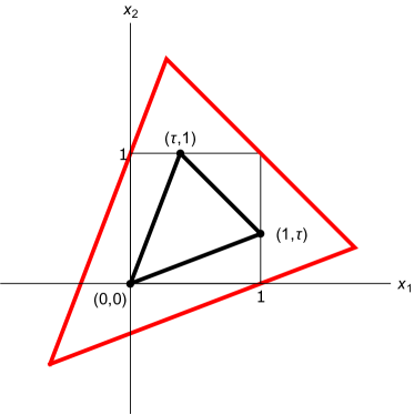
Figure 1: The case $n=2$. The golden section simplex

Combining our approach with some results of [13], we prove in [17] that $\xi_{3}(Q_{3})=3.$ Up to a change of coordinates, each extremal simplex in $Q_{3}$ coincides with the tetrahedron $S^{\prime}$ with vertices

$$(1,1,0),~{}~{}~{}(1,0,1),~{}~{}~{}(0,1,1),~{}~{}~{}(0,0,0)$$

or the tetrahedron $S^{\prime\prime}$ with vertices

$$\left(\frac{1}{2},0,0\right),~{}~{}~{}\left(\frac{1}{2},1,0\right),~{}~{}~{}\left(0,\frac{1}{2},1\right),~{}~{}~{}\left(1,\frac{1}{2},1\right).$$

In other words, if $\xi(Q_{3};S)=3,$ then either vertices of $S$ coincide with vertices of the cube and form a regular tetrahedron or coincide with the centers of opposite edges of two opposite faces of the cube and does not belong to a common plane. One can see that all axial diameters of $S^{\prime}$ and $S^{\prime\prime}$ are equal to 1. This also follows from the equality $\xi_{3}(Q_{3})=3.$ Note that ${\rm vol}(S^{\prime})=\nu_{3}=1/3,$ and ${\rm vol}(S^{\prime\prime})=1/6$.

In [35] and [45] we show that each extremal simplex for $n=2$ and $n=3$ is equisecting, i.e., the hyperplanes containing its faces cut off from the cube in outer direction from the simplex the domains of equal volumes.

The estimate $\xi_{n}(Q_{n})\geq n$ occurs to be exact in order of $n$. Indeed, let $n>2$ and let $S^{*}$ be the simplex with the zero-vertex and other $n$ vertices coinciding with the vertices of $Q_{n}$ adjacent to $(1,\ldots,1)$, i.e., with the vertices

$$(0,1,\ldots,1),~{}~{}~{}(1,0,\ldots,1),~{}~{}~{}\ldots,~{}~{}~{}(1,1,\ldots,0),~{}~{}~{}(0,0,\ldots,0)$$ (2.10)

(see [21], [24, § 3.2]). If $n\geq 3$, then $S^{*}$ has the following property (see [10, Lemma 3.3]): replacement of an arbitrary vertex of $S^{*}$ by any point of $Q_{n}$ decreases the volume of the simplex. For $n=2,3,4$ (and only in these cases), simplex $S^{*}$ has maximum volume in $Q_{n}$ (see also [10]). As it is shown in [21], if $n\geq 2$, then $d_{i}(S^{*})=1$ for every $i=1,...,n$, and therefore, thanks to (2.2), $\alpha(Q_{n};S^{*})=n.$ For this simplex,

$$\xi(Q_{n};S^{*})=\frac{n^{2}-3}{n-1}.$$

Hence, for $n>2$,

$$\xi_{n}(Q_{n})\leq\frac{n^{2}-3}{n-1}.$$ (2.11)

If $n>1$, the right-hand side of (2.11) is strictly smaller than $n+1$. Since

$$\xi_{1}(Q_{1})=1,~{}~{}~{}\xi_{2}(Q_{2})=\frac{3\sqrt{5}}{5}+1=2.3416\ldots,$$

inequality $\xi_{n}<n+1$ holds true also for $n=1,2$.

We note that if the volume of simplex $S\subset Q_{n}$ is maximal, then $\xi(Q_{n};S)\leq n+2$, see [24].

Simplices satisfying the inclusions $S\subset Q_{n}\subset nS$ were studied in [35]. The existence of such simplices for a given $n$ is equivalent to the equality $\xi_{n}(Q_{n})=n.$ This holds not for each $n$, but nowaday a unique known dimension for which $\xi_{n}(Q_{n})>n$ is $n=2$.

Thus, always $n\leq\xi_{n}(Q_{n})<n+1$, i.e., $\xi_{n}(Q_{n})-n\in[0,1)$. However, the exact values of the constant $\xi_{n}(Q_{n})$ are currently only known for $n=2$, $n=5$ and $n=9$, as well as for an infinite set of $n$ for which there exists an Hadamard matrix of order $n+1$.

In all these cases, except $n=2$, the equality $\xi_{n}(Q_{n})=n$ holds. In the noted Hadamard case, one can give the proof using the structure of Hadamard matrix of order $n+1$, see [37]. In [37], we have also discovered the exact values of $\xi_{n}(Q_{n})$ for $n=5$ and $n=9$ and constructed several infinite families of extremal simplices for $n=5,7,9$.

We call a nondegenerate simplex $S\subset Q_{n}$ perfect provided $\xi(Q_{n};S)=\xi_{n}(Q_{n})$ and the cube $Q_{n}$ is inscribed into the simplex $\xi(Q_{n};S)\,S$. For a long time, only two dimensions were known, namely $n=1$ and $n=3$, for which such simplices exist. Every three-dimensional perfect simplex is similar to $S^{\prime\prime}$. In Fig. 2 it can be seen that all vertices of $Q_{3}$ belong to the boundary of the simplex $3S^{\prime\prime}$.

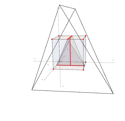
Figure 2: The case $n=3$. Simplex $S^{\prime\prime}$

On the contrary, simplex $S^{\prime}$ is not perfect, While $Q_{3}\subset 3S^{\prime}$, only four vertices of the cube lie on the boundary of the simplex $3S^{\prime}$. See Fig. 3.

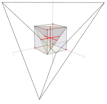
Figure 3: The case $n=3$. Simplex $S^{\prime}$

It was shown in [37] that perfect simplices do exist also in ${\mathbb{R}}^{5}$.

As we have mentioned above, nowaday $n=2$ is a unique known dimension for which $\xi_{n}(Q_{n})>n.$

Let us also note that dimension $n=2$ remains the only even positive integer where we know the sharp value of the constant $\xi_{n}(Q_{n})$. Also, it is still unknown whether there exists an even $n$ such that $\xi_{n}(Q_{n})=n.$ The best of known today upper bounds for $n=4$ and $n=6$ are

$$\xi_{4}(Q_{4})\leq\frac{19+5\sqrt{13}}{9}=4.1141\ldots,\quad\xi_{6}(Q_{6})<6.0166.$$

(see [33], [34]). Using simplices of maximum volume in the cube, A.Yu. Ukhalov perfomed computer calculations to get as accurate upper bounds for $\xi_{n}(Q_{n})$ as possible; the results for $n\leq 118$ are given in [36] and also in the survey paper [43].

Let us note that inequality $\xi_{n}(K)\leq n+2$ holds for an arbitrary convex body $K\subset{\mathbb{R}}^{n}$. This is immediate from the following proposition proven by M. Lassak [14]: If $S$ is a maximum volume simplex contained in $K$, then $\xi(K;S)\leq n+2.$ In other words, we have

$$S\subset K\subset(n+2)S.$$ (2.12)

Note that this statement easily follows from formula (1.10). In fact, because $S\subset K$ has maximum volume, we have $|\Delta_{j}(x)|\leq|\Delta|$ for any $j=1,\ldots,n+1$ and $x\in K.$ It suffices to use the relation (1.1) between determinants and volumes of simplices. Thanks to (1.3),

$$-\lambda_{j}(x)\leq|\lambda(x)|=\frac{|\Delta_{j}(x)|}{|\Delta|}\leq 1,\quad x\in K.$$

Thus, by (1.10), we obtain

$$\xi(K;S)=(n+1)\max_{1\leq k\leq n+1}\max_{x\in K}(-\lambda_{k}(x))+1\leq n+2.$$

This approach was used by the author in [24] in the case $K=Q_{n}$.

3. The values of $\alpha(B_{n};S)$ and $\xi(B_{n};S)$

In this section we discuss characteristics associated with the absorption of a Euclidean ball by a homothetic image of a simplex (with or without translation). Replacing a cube with a ball makes many questions much more simple. However, geometric interpretation of general results has a certain interest also in this particular case. Besides, we will note some new applications of the basic Lagrange polynomials.

Given an $n$-dimensional simplex $S$, let us introduce the following geometric characteristics. The  inradius of $S$ is the maximum of the radii of balls contained within $S$. The center of this unique maximum ball is called the incenter of $S$. The boundary of the maximum ball is a sphere that has a single common point with each $(n-1)$-dimensional face of $S$. By the circumradius of S we mean the minimum of the radii of balls containing $S$. Note that the boundary of this unique minimal ball contains all the vertices of $S$ if and only if its center lies inside the simplex.

The inradius $r$ and the circumradius $R$ of a simplex $S$ satisfy the so-called Euler inequality

$$R\geq nr.$$ (3.1)

Equality in (3.1) takes place if and only if $S$ is a regular simplex. For the proof of the Euler inequality, its history and various generalizations we refer the reader to [12], [58] and [56].

Let us note that the Euler inequality is equivalent to the following statement: Suppose $B$ is a ball with radius $r_{1}$ and $B^{*}$ is a ball with radius $r_{2}$. If $B\subset S\subset B^{*}$, then $r_{2}\geq nr_{1}.$ Equality takes place if and only if $S$ is a regular simplex inscribed into $B^{*}$ and $B$ is the ball inscribed into $S$. Another equivalent form of these propositions is given by Theorem 3.3.

Also we remark that the analog of the above property for parallelotopes is expressed by Corollary 2.5.

We turn to presentation of some computational formulae for the quantities $\alpha(B_{n};S)$ and $\xi(B_{n};S)$ proven in [28]. Let $x^{(1)},$ $\ldots,$ $x^{(n+1)}$ be the vertices and $\lambda_{1},$ $\ldots,$ $\lambda_{n+1}$ be the basic Lagrange polynomials of a nondegenerate simplex $S\subset{\mathbb{R}}^{n}$. As usual, $l_{ij}$ are the coefficients of $\lambda_{j}.$ See formulas from Section 1.

Given $j\in\{1,...,n+1\}$, let $\Gamma_{j}$ be the $(n-1)$-dimensional hyperplane determined by the equation $\lambda_{j}(x)=0$, and let $\Sigma_{j}$ be the $(n-1)$-dimensional face of $S$ contained in $\Gamma_{j}$. We let $h_{j}$ denote the height of $S$ conducted from $x^{(j)}$ onto $\Gamma_{j}$, and we let $r$ denote the inradius of $S$. By $\sigma_{j}$ we denote $(n-1)$-dimensional measure of $\Sigma_{j}$. Finally, we put $\sigma=\sum\limits_{j=1}^{n+1}\sigma_{j}$.

In [28] we show that the value $\alpha(B_{n};S)$ can be calculated in various ways.

Theorem 3.1. The following equalities hold:

$$\alpha(B_{n};S)=\sum_{j=1}^{n+1}\left(\sum_{i=1}^{n}l_{ij}^{2}\right)^{1/2},$$ (3.2)

$$\alpha(B_{n};S)=\sum_{j=1}^{n+1}\frac{1}{h_{j}},$$ (3.3)

$$\alpha(B_{n};S)=\frac{1}{r},$$ (3.4)

$$\alpha(B_{n};S)=\frac{\sigma}{n\,{\rm vol}(S)}.$$

From (3.3) and (3.4) we get

$$\frac{1}{r}=\sum_{j=1}^{n+1}\frac{1}{h_{j}}.$$

This geometric relation (which evidently can be obtained in the direct way) occurs to be equivalent to general formula (1.11) for $\alpha(K;S)$ in the case when the convex body $K$ coincide with the unit ball.

It is interesting to compare (3.2) with the formula

$$\alpha(Q_{n}^{\prime};S)=\sum_{i=1}^{n}\sum_{j=1}^{n+1}|l_{ij}|.$$

for the cube $Q_{n}^{\prime}=[-1,1]^{n}$ (see Corollary 2.2). Since $B_{n}\subset Q_{n}^{\prime}$, it follows that $\alpha(B_{n};S)\leq\alpha(Q_{n}^{\prime};S)$. Of course, analytically, this inequality is immediate from (3.2) and the above formula for $\alpha(Q_{n}^{\prime};S)$.

In turn, the inradius $r$ and the incenter $z$ of a simplex $S$ can be calculated as follows:

$$r=\frac{1}{\sum\limits_{j=1}^{n+1}\left(\sum\limits_{i=1}^{n}l_{ij}^{2}\right)^{1/2}},\quad z=\frac{1}{\sum\limits_{j=1}^{n+1}\left(\sum\limits_{i=1}^{n}l_{ij}^{2}\right)^{1/2}}\sum\limits_{j=1}^{n+1}\left(\sum\limits_{i=1}^{n}l_{ij}^{2}\right)^{1/2}x^{(j)}.$$

For arbitrary $x^{(0)}$ and $\varrho>0$, the quantity $\alpha\left(B(x^{(0)};\varrho);S\right)$ one can calculate using the equality $\alpha(B(x^{(0)};\varrho);S)$ $=$ $\varrho\alpha(B_{n};S)$.

The general formula (1.10) for $\xi(K;S)$ in the case $K=B\left(x^{(0)};\varrho\right)$ provides the following (see [28]).

Theorem 3.2. If $B\left(x^{(0)};\varrho\right)\not\subset S$, we have

$$\xi\left(B\left(x^{(0)};\varrho\right);S\right)=(n+1)\max_{1\leq j\leq n+1}\left[\varrho\left(\sum_{i=1}^{n}l_{ij}^{2}\right)^{1/2}-\sum_{i=1}^{n}l_{ij}x_{i}^{(0)}-l_{n+1,j}\right]+1.$$ (3.5)

In particular, in the case $B_{n}\not\subset S$

$$\xi(B_{n};S)=(n+1)\max_{1\leq j\leq n+1}\left[\left(\sum_{i=1}^{n}l_{ij}^{2}\right)^{1/2}-l_{n+1,j}\right]+1.$$ (3.6)

Now we turn to lower bounds for $\alpha(B_{n};S)$ and $\xi(B_{n};S)$ for $S\subset B_{n}.$ It is easy to show that the Euler inequality is equivalent to the following statement.

Theorem 3.3. If $S\subset B_{n}$, then $\alpha(B_{n};S)\geq n.$ The equality $\alpha(B_{n};S)=n$ holds true if and only if $S$ is a regular simplex inscribed into $B_{n}$.

Recall that the minimum value of $\alpha(Q_{n};S)$ for $S\subset Q_{n}$ is also equal to $n$ (see (2.6)). This value corresponds to those and only those $S\subset Q_{n}$ for which every axial diameter $d_{i}(S)$ is equal to $1$. The latter property is fulfilled for the maximum volume simplices in $Q_{n}$, but, if $n>2$, not for the only ones.

If $S\subset B_{n}$, then $\xi(B_{n};S)\geq n.$ The equality $\xi(B_{n};S)=n$ takes place if and only if $S$ is a regular simplex inscribed into $B_{n}$. These statements immediately follow from Theorem 3.3 and the inequality $\xi(B_{n};S)\geq\alpha(B_{n};S)$. Paper [28] contains also the direct arguments without applying the Euler inequality that was used in [28] to obtain the estimate $\alpha(B_{n};S)\geq n$.

Now, let us consider an analog of the quantity $\xi_{n}(Q_{n})$, the quantity $\xi_{n}(B_{n})$. In accordance with Definition 1.3,

$$\xi_{n}(B_{n})=\min\{\xi(B_{n};S):\,S\mbox{ is an $n$-dimensional simplex,}\,S\subset B_{n},\,{\rm vol}(S)\neq 0\}.$$

While many problems concerning $\xi_{n}(Q_{n})$ yet have not been solved (see Section 2), the problem on numbers $\xi_{n}(B_{n})$ turns out to be simple. For any $n$, we have $\xi_{n}(B_{n})=n$. The only simplex $S\subset B_{n}$ extremal with respect to $\xi_{n}(B_{n})$ is an arbitrary regular simplex inscribed into $B_{n}$.

Let us note that, thanks to (1.7), for every interpolation projector $P:C(B_{n})\to\Pi_{1}\left({\mathbb{R}}^{n}\right)$ and the corresponding simplex $S\subset B_{n}$, the following inequalities

$$\frac{n+1}{2n}\Bigl{(}\|P\|_{B_{n}}-1\Bigr{)}+1\leq\xi(B_{n};S)\leq\frac{n+1}{2}\Bigl{(}\|P\|_{B_{n}}-1\Bigr{)}+1$$ (3.7)

hold. Furthermore, if there exists an $1$-point in $B_{n}$ with respect to $S$ (see Section 1), then the right-hand inequality in (3.7) becomes an equality. Hence,

$$\frac{n+1}{2n}\Bigl{(}\theta_{n}(B_{n})-1\Bigr{)}+1\leq\xi_{n}(B_{n})=n\leq\frac{n+1}{2}\Bigl{(}\theta_{n}(B_{n})-1\Bigr{)}+1.$$ (3.8)

Starting from $n=5$, the right-hand inequality in (3.7) is strict, while for $1\leq n\leq 4$ it turns into equality. This fact is noted in Section 7. Here is another argument, but also using some of the properties below. Since we know the precise value of $\theta_{n}(B_{n})$ (see Section 9), the cases $1\leq n\leq 5$ are cheking directly. The result for $n\geq 6$ follows from the estimate $\theta_{n}(B_{n})\geq\sqrt{n}$, since then

$$n<\frac{n+1}{2}\Bigl{(}\sqrt{n}-1\Bigr{)}+1.$$

4. Estimates for $\theta_{n}(Q_{n})$

Despite the apparent simplicity of formulation, the problem of finding exact values of $\theta_{n}(Q_{n})$ is very difficult. Since 2006, these values are known only for $n=1,2,3,$ and $7$. Namely,

$$\theta_{1}(Q_{1})=1,\quad\theta_{2}(Q_{2})=\frac{2\sqrt{5}}{5}+1=1.8944\ldots,\quad\theta_{3}(Q_{3})=2,\quad\theta_{7}(Q_{7})=\frac{5}{2}.$$

Note that for each $n=1,2,3,7$ the right-hand relation in (1.8) becomes an equality:

$$\xi_{n}(Q_{n})=\frac{n+1}{2}\left(\theta_{n}(Q_{n})-1\right)+1.$$ (4.1)

If $n=1,3,$ or $7$, then an equality takes place also in (2.7), i. e.,

$$\theta_{n}(Q_{n})=3-\frac{4}{n+1}.$$

For $1\leq n\leq 3$, the simplices corresponding to minimal projectors are just the same that the extremal simplices with respect to $\xi_{n}(Q_{n})$, see Section 2. In the seven-dimensional case, the nodes of minimal projector appear from a unique (up to equivalence) Hadamard matrix of order $8$. The proofs are given in original paper [19] and also in [24] and [46].

Clearly, $\theta_{1}(Q_{1})=1$. This value can be found also from (1.8). For any projector, there is a $1$-vertex $Q_{1}$ relative to the corresponding simplex (which is a segment). Hence, we have (4.1). Now $\xi_{1}(Q_{1})=1$ implies $\theta_{1}(Q_{1})=1.$ The nodes of a unique minimal projector are 0 and 1. For the most complicated cases $n=2,3,$ see [24].

Let us turn to the case $n=7$. Since $8$ is an Hadamard number, there exists a seven-dimensional regular simplex having vertices at vertices of the cube. We can take the simplex with the vertices

$$(1,1,1,1,1,1,1),~{}~{}~{}(0,1,0,1,0,1,0),~{}~{}~{}(0,0,1,1,0,0,1),~{}~{}~{}(1,0,0,1,1,0,0),$$

$$(0,0,0,0,1,1,1),~{}~{}~{}(1,0,1,0,0,1,0),~{}~{}~{}(1,1,0,0,0,0,1),~{}~{}~{}(0,1,1,0,1,0,0).$$

The equality $\xi_{7}(Q_{7})=7$ (see Section 2) and inequality

$$\xi_{n}(Q_{n})\leq\frac{n+1}{2}\left(\theta_{n}(Q_{n})-1\right)+1$$

imply $\theta_{7}(Q_{7})\geq\frac{5}{2}$. But for the corresponding projector, $\|P\|_{Q_{7}}=\frac{5}{2}$. Therefore, $\theta_{7}=\frac{5}{2}$, and this projector is minimal.

Calculations seems to be more easy if we make use of similarity reasons. Let us take the cube $Q_{7}^{\prime}=[-1,1]$ and consider the projector $P:C(Q_{7}^{\prime})\to\Pi_{1}\left({\mathbb{R}}^{7}\right)$ constructed from the Hadamard matrix

$${\bf H}_{8}=\left(\begin{array}[]{cccccccc}1&1&1&1&1&1&1&1\\ -1&1&-1&1&-1&1&-1&1\\ -1&-1&1&1&-1&-1&1&1\\ 1&-1&-1&1&1&-1&-1&1\\ -1&-1&-1&-1&1&1&1&1\\ 1&-1&1&-1&-1&1&-1&1\\ 1&1&-1&-1&-1&-1&1&1\\ -1&1&1&-1&1&-1&-1&1\end{array}\right).$$

(This matrix is unique up to the equivalence of Hadamard matrix of order 8.) Suppose the nodes of $P$ are written in the rows of this matrix except the last column. Since ${\bf H}_{8}^{-1}$ $=$ $({1}/{8}){\bf H}_{8}^{T},$ coefficients of $\lambda_{j}$ form the $j$th row of $({1}/{8}){\bf H}_{8}:$

$$\lambda_{1}(x)=\frac{1}{8}\left(x_{1}+x_{2}+x_{3}+x_{4}+x_{5}+x_{6}+x_{7}+1\right),$$

$$\lambda_{2}(x)=\frac{1}{8}\left(-x_{1}+x_{2}-x_{3}+x_{4}-x_{5}+x_{6}-x_{7}+1\right),$$

and so on. Using (1.6), we get $\|P\|_{Q_{7}^{\prime}}={5}/{2}$, and, thanks to the above approach, $\theta_{7}(Q^{\prime}_{7})={5}/{2}.$

However, $n=7$ is the biggest $n$ such that (i) $n+1$ is an Hadamard number and (ii) (2.8) holds provided $P$ corresponds to a regular simplex inscribed into the cube.

Now let us note some upper bounds for $\theta_{n}(Q_{n})$. For $n\geq 3$, the projector with nodes (2.10) satisfies $\|P\|_{Q_{n}}\leq({n+1})/{2}$ with the equality for odd $n$ ([16], [24]). Therefore, if $n\neq 2$, then

$$\theta_{n}(Q_{n})\leq\frac{n+1}{2}.$$

Recall that $h_{n}$ denotes the maximum value of a determinant of order $n$ with entries $0$ or $1$ (see Definition 1.9). Suppose $P$ corresponds to a maximum volume simplex $S\subset Q_{n}$ with some vertex coinciding with a vertex of the cube. Then

$$\|P\|_{Q_{n}}\leq\frac{2h_{n+1}}{h_{n}}+1.$$ (4.2)

Hence,

$$\theta_{n}(Q_{n})\leq\frac{2h_{n+1}}{h_{n}}+1$$

for all $n$ and also $\theta_{n}(Q_{n})\leq\sqrt{2n+3}+1$, provided $n+1$ is an Hadamard number (see [31]). Earlier (see [16] and [24]) it was proved that in the Hadamard case $\xi_{n}(Q_{n})\leq\sqrt{n+1}$. Let us give here the proof from [31] essentially making use of the structure of an Hadamard matrix.

Theorem 4.1. Let $n+1$ be an Hadamard number, and let $S$ be an $n$-dimensional regular simplex having the vertices at vertices of $Q_{n}^{\prime}$. Then, for the corresponding interpolation projector $P:C(Q_{n}^{\prime})\to\Pi_{1}({\mathbb{R}}^{n})$, we have

$$\|P\|_{Q_{n}^{\prime}}\leq\sqrt{n+1}.$$ (4.3)

Proof. Let $x^{(1)},\ldots,x^{(n+1)}$ be the vertices and let $\lambda_{1},\ldots,\lambda_{n+1}$ be the basic Lagrange polynomials of the simplex. Thanks to the theorem’s hypothesis, the vertex matrix $\bf S$ is an Hadamard matrix of order $n+1$ with the last column consisting of $1$’s.

Let us show that

$$\sum_{j=1}^{n+1}\lambda_{j}(x)^{2}=\frac{||x||^{2}+1}{n+1}~{}~{}~{}\text{for every}~{}~{}~{}x\in{\mathbb{R}}^{n}.$$ (4.4)

Let $y=(x_{1},\ldots,x_{n},1)\in{\mathbb{R}}^{n+1}.$ The coefficients of $\lambda_{j}$ form the $j$th column of ${\bf S}^{-1}$. Since $\bf S$ is an Hadamard matrix, it satisfies (1.14), whence

$$\lambda_{j}(x)=\frac{1}{n+1}\langle h^{(j)},y\rangle.$$

Further, ${h^{(j)}}/{\sqrt{n+1}}$ form an orthonormalized basis of ${\mathbb{R}}^{n+1},$ therefore,

$$y=\sum_{j=1}^{m}\frac{\langle h^{(j)},y\rangle}{\sqrt{n+1}}\frac{h^{(j)}}{\sqrt{n+1}},\quad\langle y,y\rangle=\sum_{j=1}^{n+1}\frac{\langle h^{(j)},y\rangle^{2}}{n+1}.$$

From this, we have

$$||x||^{2}+1=\langle y,y\rangle=\sum_{j=1}^{n+1}\frac{\langle h^{(j)},y\rangle^{2}}{n+1}=(n+1)\sum_{j=1}^{n+1}\lambda_{j}(x)^{2}$$

proving (4.4).

If $x$ is a vertex of $Q_{n}^{\prime}$, then $||x||^{2}=n$ and (4.4) implies $\sum\lambda_{j}(x)^{2}=1.$ Applying Cauchy inequality, for each $x\in{\rm ver}(Q_{n}^{\prime})$, we have

$$\sum_{j=1}^{n+1}|\lambda_{j}(x)|\leq\left(\sum_{j=1}^{n+1}\lambda_{j}(x)^{2}\right)^{\frac{1}{2}}\cdot\sqrt{n+1}=\sqrt{n+1}.$$

Now, let $P:C(Q_{n}^{\prime})\to\Pi_{1}({\mathbb{R}}^{n})$ be an interpolation projector corresponding to $S$. Then, thanks to (1.6),

$$\|P\|_{Q_{n}^{\prime}}=\max_{x\in{\rm ver}(Q_{n}^{\prime})}\sum_{j=1}^{n+1}|\lambda_{j}(x)|\leq\sqrt{n+1}$$

completing the proof of the theorem. $\Box$

By similarity reasons, Theorem 4.1 overcomes to any $n$-dimensional cube, e. g., to the cube $Q_{n}=[0,1]^{n}$. Thus, if $n+1$ is an Hadamard number, then $\theta_{n}(Q_{n})\leq\sqrt{n+1}.$

We can slightly improve this estimate by using interpolation on a ball.

Let $p_{n}=\max\{\psi(a),\psi(a+1)\}$ where

$$\psi(t):=\frac{2\sqrt{n}}{n+1}\Bigl{(}t(n+1-t)\Bigr{)}^{1/2}+\left|1-\frac{2t}{n+1}\right|,\quad a=\left\lfloor\frac{n+1}{2}-\frac{\sqrt{n+1}}{2}\right\rfloor.$$

Now, let us assume that $n+1$ is an Hadamard number. Consider an interpolation projector $P$ with the nodes at those vertices of the cube $Q_{n}^{\prime}$ that form a regular simplex $S$. Since $Q_{n}^{\prime}$ is inscribed into the unit ball $B_{n}$, simplex $S$ is also inscribed into $B_{n}$. It remains to apply formula (1.5) for the projector’s norm both on the cube and on the ball:

$$\|P\|_{Q_{n}^{\prime}}=\max_{x\in Q_{n}^{\prime}}\sum_{j=1}^{n+1}|\lambda_{j}(x)|\leq\max_{x\in B_{n}}\sum_{j=1}^{n+1}|\lambda_{j}(x)|=\|P\|_{B_{n}}=p_{n}\leq\sqrt{n+1}.$$

(For the equality $\|P\|_{B_{n}}=p_{n}$ and the final estimate, we refer the reader to Section 7.) Hence,

$$\theta_{n}(Q_{n})\leq p_{n}\leq\sqrt{n+1}.$$

The equality $\|P\|_{Q_{n}^{\prime}}=\sqrt{n+1}$ may hold as for all regular simplices having vertices at vertices of the cube $(n=1,n=3)$, as for some of them $(n=15),$ or may not be executed at all.

As it is shown in Section 6, for each $n$, $\theta_{n}(Q_{n})\geq\sqrt{n-1}/e.$ Therefore, if $n+1$ is an Hadamard number, then

$$\frac{\sqrt{n-1}}{e}\leq\theta_{n}(Q_{n})\leq\sqrt{n+1}.$$

The upper bounds of $\theta_{n}(Q_{n})$ for special $n$ were improved by A. Ukhalov and his students with the help of computer methods. In particular, simplices of maximum volume in the cube were considered. In all situations where $n+1$ is an Hadamard number, the full set of Hadamard matrices of the corresponding order was used. In particular, to obtain an estimate for $\theta_{23}$, all existing $60$ Hadamard matrices of order $24$ were considered. To estimate $\theta_{27}$, we have to consider $487$ Hadamard matrices of order $28$. Known nowaday upper estimates for $1\leq n\leq 27$ are given in [46]. (Here, for brevity, $\theta_{n}=\theta_{n}(Q_{n})$.)

$$\theta_{1}=1,\quad\theta_{2}=\frac{2\sqrt{5}}{5}+1,\quad\theta_{3}=2,\quad\theta_{4}\leq\frac{3(4+\sqrt{2})}{7},\quad\theta_{5}\leq 2.448804,$$

$$\theta_{6}\leq 2.6000\ldots,\quad\theta_{7}=\frac{5}{2},\quad\theta_{8}\leq\frac{22}{7},\quad\theta_{9}\leq 3,\quad\theta_{10}\leq\frac{19}{5},\quad\theta_{11}\leq 3,$$

$$\theta_{12}\leq\frac{17}{5},\quad\theta_{13}\leq\frac{49}{13},\quad\theta_{14}\leq\frac{21}{5},\quad\theta_{15}\leq\frac{7}{2},\quad\theta_{16}\leq\frac{21}{5},\quad\theta_{17}\leq\frac{139}{34},$$

$$\theta_{18}\leq 5.1400\ldots,\quad\theta_{19}\leq 4,\quad\theta_{20}\leq 4.68879\ldots,\quad\theta_{21}\leq\frac{251}{50},\quad\theta_{22}\leq\frac{1817}{335},$$

$$\theta_{23}\leq\frac{9}{2},\quad\theta_{24}\leq\frac{103}{21},\quad\theta_{25}\leq 5,\quad\theta_{26}\leq\frac{474}{91},\quad\theta_{27}\leq 5.$$

Note that $n$-dimensional regular simplices with vertices at the vertices of the cube can be located differently with respect to the vertices and faces of the cube. This is quite evident when the norms of the corresponding projectors are different. But this is also possible if regular simplices generate the same norms. In [31] we describe an approach based on comparison of $\mu$-vertices of the cube with respect to various simplices.

Recall that a $\mu$-vertex of the cube $Q$ with respect to a simplex $S\subset Q$ is such a vertex $x$ of the cube that for the corresponding projector $P=P_{S}$ we have $\|P\|_{Q}=\sum|\lambda_{j}(x)|$ and exactly $\mu$ numbers $\lambda_{j}(x)$ are negative (see Definition 1.7). Of course, simplices which have different sets of $\mu$-vertices with respect to the containing cube, are differently located in the cube, even if they have the same projector’s norms. These simplices are non-equivalent in the following sense: one of them cannot be mapped into another by an orthogonal transform which maps the cube into itself. Let us give some examples for the case $Q=Q_{n}^{\prime}.$

While obtaining estimates for minimal norms of projectors, in [38] various $n$-dimensional regular simplices arising from different Hadamard matrices of order $n+1$ were calculated. For $n=15$, the order of matrices is equal to $16$. Up to equivalence, there are exactly five Hadamard matrices. They correspond to five simplices described in Table 1.

Table 1: Regular simplices for $n=15$

$\begin{array}[]{|c|c|c|c|}\hline\cr S&{\|P\|}_{Q_{15}^{\prime}}&\mbox{Values }\ \mu&\mbox{ Number of}\ \mu\mbox{-vertices}\\ \hline\cr S_{1}&4&6&m_{6}=448\\ S_{2}&4&6&m_{6}=192\\ S_{3}&4&6&m_{6}=64\\ S_{4}&\frac{7}{2}&4,5,6,8&m_{4}=896,m_{5}=1344,m_{6}=5376,m_{8}=1344\\ S_{5}&\frac{7}{2}&4,5,6,8&m_{4}=896,m_{5}=1344,m_{6}=5376,m_{8}=1344\\ \hline\cr\end{array}$

By $m_{\mu}$ we denote a number of $\mu$-vertices of the cube $Q_{n}^{\prime}$ with respect to every simplex. For the rest $1\leq\mu\leq 15$, excepting the given in Table 1, values $m_{\mu}$ are zero. Every simplex $S_{1}$, $S_{2}$, and $S_{3}$ generates the same projector’s norm and has only $6$-vertices. But the numbers of $6$-vertices for them are different; hence, these simplices are pairwise non-equivalent. Each of them also is non-equivalent as to $S_{4}$, so as to $S_{5}.$ The latter simplices generates equal norms and have the same sets of $\mu$-vertices. Also we have $\theta_{15}\leq{7}/{2}=3.5$. This is more exact than the estimate $\theta_{15}(Q_{15})\leq 4$ provided by (4.3).

Another example given in [31] is related to $n=23.$ Regular inscribed simplices were built from the available 60 pairwise non-equivalent Hadamard matrices of order $24$. For all simplices, excepting ones with the numbers 16, 53, 59, and 60, the projector norm equals ${14}/{3}=4.6666\ldots$, while for each of these four simplices the projector norm is ${9}/{2}=4.5$. In particular, we have $\theta_{23}(Q_{23})\leq 4.5$ (which was also noted in [38]). This inequality is more exact than the estimate $\theta_{23}(Q_{23})\leq\sqrt{24}=4.8989\ldots$. Each of the four exceptional simplices is not equivalent to any of the 56 others.

Despite the possible differs, for all regular simplices with vertices at the vertices of the cube, inequality (4.3) holds. The inscribed regular simplices satisfying $\|P\|_{Q_{n}^{\prime}}=\sqrt{n+1}$ exist at least for $n=1$, $n=3$, and $n=15.$ The problem of full description of dimensions $n$ with such property is still open.

The best nowaday known lower bound of $\theta_{n}(Q_{n})$ has the form

$$\theta_{n}(Q_{n})\geq\max\left[3-\frac{4}{n+1},\,\chi_{n}^{-1}\left(\frac{1}{\nu_{n}}\right)\right].$$ (4.5)

Here $\chi_{n}$ is the standardized Legendre polynomial of degree $n$, see Section 5.

The values of the right-hand side of (4.5) for $1\leq n\leq 54$ are given in [46]. Inequality

$$\chi_{n}^{-1}\left(\frac{1}{\nu_{n}}\right)>3-\frac{4}{n+1}$$

takes place for $n\geq 53$. On estimates via the function $\chi_{n}^{-1}$ see Section 6.

As noted in Section 1 (see the right-hand relation in (1.7)), the inequality

$$\xi_{n}(Q_{n})\leq\frac{n+1}{2}\left(\theta_{n}(Q_{n})-1\right)+1$$ (4.6)

is true for any $n$. So far, we know only four values of $n$ for which this relation becomes an equality: $n=1,2,3$, and $7$. These are exactly the cases in which we know the exact values of $\theta_{n}(Q_{n})$ and $\xi_{n}(Q_{n})$. In [33] the authors conjectured that the minimum of $n$ for which inequality (4.6) is strict is $4.$ This is still an open problem.

We note that, thanks to the equivalence $\xi_{n}(Q_{n})\asymp n$ and inequality $\theta_{n}\geq c\sqrt{n}$, for all sufficiently large $n$, we have

$$\xi_{n}(Q_{n})<\frac{n+1}{2}\left(\theta_{n}(Q_{n})-1\right)+1.$$ (4.7)

Let $n_{0}$ be the minimal natural number such that for all $n\geq n_{0}$ inequality (4.7) holds. The problem about the exact value of $n_{0}$ is very difficult. The known lower and upper bounds differ quite significantly. From the preceding, we have the estimate $n_{0}\geq 8.$ In 2009 we proved that $n_{0}\leq 57$ (see [19], [24, § 3.7]). A sufficient condition for the validity of (4.7) for $n>2$ is the inequality

$$\chi_{n}\left(\frac{3n-5}{n-1}\right)\cdot\nu_{n}<1.$$ (4.8)

It was proved in [19] that (4.8) is satisfied for $n\leq 57$. Later calculations allowed the upper bound of $n_{0}$ to be slightly lowered. These results are described in [38] where it is noted that $n_{0}\leq 53$. In other words, inequality (4.7) is satisfied at least starting from $n=53$. Note that a better estimate from above for $n_{0}$ is an open problem.

5. Legendre polynomials and the measure of $E_{n,\gamma}$

The standardized Legendre polynomial of degree $n$ is the function

$$\chi_{n}(t)=\frac{1}{2^{n}n!}\left[(t^{2}-1)^{n}\right]^{(n)}$$

(Rodrigues’ formula). For properties of $\chi_{n}$ see, e.g., [52],[53]. Legendre polynomials are orthogonal on the segment $[-1,1]$ with the weight $w(t)\equiv 1.$ The first standardized Legendre polynomials are

$$\chi_{0}(t)=1,\quad\chi_{1}(t)=t,\quad\chi_{2}(t)=\frac{1}{2}\left(3t^{2}-1\right),\quad\chi_{3}(t)=\frac{1}{2}\left(5t^{3}-3t\right),$$

$$\chi_{4}(t)=\frac{1}{8}\left(35t^{4}-30t^{2}+3\right),\quad\chi_{5}(t)=\frac{1}{8}\left(63t^{5}-70t^{3}+15t\right).$$

We have

$$\chi_{n+1}(t)=\frac{2n+1}{n+1}\,t\chi_{n}(t)-\frac{n}{n+1}\,\chi_{n-1}(t).$$ (5.1)

This implies $\chi_{n}(1)=1$. If $n\geq 1$, then $\chi_{n}(t)$ increases as $t\geq 1$. The latter properties also easily follow from (5.2).

We let $\chi_{n}^{-1}$ denote the function inverse to $\chi_{n}$ on the semi-axis $[1,+\infty)$.

The appearance of Legendre polynomials in the circle of our questions is due to some their property. For $\gamma\geq 1$, let us define the set

$$E_{n,\gamma}:=\left\{x\in{\mathbb{R}}^{n}:\sum_{j=1}^{n}|x_{j}|+\left|1-\sum_{j=1}^{n}x_{j}\right|\leq\gamma\right\}.$$

In [16] we proved such a statement (the proof is also given in [24] and [46]).

Theorem 5.1. The following equalities hold:

$${\rm mes_{n}}(E_{n,\gamma})=\frac{1}{2^{n}n!}\sum_{i=0}^{n}{n\choose i}^{2}(\gamma-1)^{n-i}(\gamma+1)^{i}=\frac{\chi_{n}(\gamma)}{n!}.$$ (5.2)

Proof. First let us establish the left-hand equality in (5.2). Let

$$E^{(1)}=\{x\in E_{n,\gamma}:\sum x_{i}>1\},~{}~{}~{}~{}E^{(2)}=\{x\in E_{n,\gamma}:\sum x_{i}\leq 1\}.$$

Let us find sequentially $m_{1}={\rm mes_{n}}(E^{(1)})$ and $m_{2}={\rm mes_{n}}(E^{(2)}).$

Temporarily fix $k$, $1\leq k\leq n$, and consider a non-empty subset $G\subset E^{(1)}$ consisting of all points $x=(x_{1},...,x_{n})$ such that $x_{1},\ldots,x_{k}\geq 0$ and $x_{k+1},\ldots,x_{n}<0$. Let $y_{i}=x_{i}$ for $i=1,...,k$, $y_{i}=-x_{i}$ for $i=k+1,...,n$, and let $y=(y_{1},...,y_{n})$. Then

$$G=\left\{y:1+y_{k+1}+\ldots+y_{n}\leq y_{1}+\ldots+y_{k}\leq\frac{\gamma+1}{2},\ y_{i}\geq 0\right\},$$

hence

$${\rm mes_{n}}(G)=\int\limits_{1}^{\alpha}\,dy_{1}\int\limits_{1}^{\alpha-y_{1}}\,dy_{2}\ldots\int\limits_{1}^{\alpha-y_{1}-\ldots-y_{k-1}}\,dy_{k}\cdot$$

$$\cdot\int\limits_{0}^{y_{1}+\ldots+y_{k}-1}\,dy_{k+1}\int\limits_{0}^{y_{1}+\ldots+y_{k}-1-y_{k+1}}\,dy_{k+2}\ldots\int\limits_{0}^{y_{1}+\ldots+y_{k}-1-y_{k+1}-\ldots-y_{n-1}}\,dy_{n}.$$

Throughout the proof, $\alpha=(\gamma+1)/2.$ If $b>0$, then

$$\int\limits_{0}^{b}\,dz_{1}\int\limits_{0}^{b-z_{1}}\,dz_{2}\ldots\int\limits_{0}^{b-z_{1}-\ldots-z_{l-1}}\,dz_{l}=\frac{b^{l}}{l!},$$

so

$${\rm mes_{n}}(G)=$$

$$=\int\limits_{1}^{\alpha}\,dy_{1}\int\limits_{1}^{\alpha-y_{1}}\,dy_{2}\ldots\int\limits_{1}^{\alpha-y_{1}-\ldots-y_{k-1}}\frac{1}{(n-k)!}{\left(y_{1}+\ldots+y_{k}-1\right)}^{n-k}\,dy_{k}=$$

$$=\left(\int\limits_{\ y_{1}+\ldots+y_{k}\leq\alpha}-\int\limits_{y_{1}+\ldots+y_{k}\leq 1}\right)\frac{1}{(n-k)!}{(y_{1}+\ldots+y_{k}-1)}^{n-k}\,dy_{1}\ldots\,dy_{k}=$$

$$=J_{1}-J_{2}.$$

The first integral equals

$$J_{1}=\sum_{j=1}^{k}(-1)^{j+1}\frac{(\alpha-1)^{n-k+j}}{(n-k+j)!}\frac{\alpha^{k-j}}{(k-j)!}+\frac{(-1)^{n+k}}{n!}.$$

The value of $J_{2}$ appears from this expression if instead of $\alpha$ we take 1. Consequently,

$${\rm mes_{n}}(G)=J_{1}-J_{2}=\sum_{j=1}^{k}(-1)^{j+1}\frac{(\alpha-1)^{n-k+j}}{(n-k+j)!}\frac{\alpha^{k-j}}{(k-j)!}=$$

$$=\frac{(-1)^{k+1}}{n!}\sum_{i=0}^{k-1}{n\choose i}(\alpha-1)^{n-i}(-\alpha)^{i}.$$

Clearly, the set $E^{(1)}$ is the union of all pairwise disjoint sets $G$ with various $k=1,\ldots,n,$. Therefore, the measure of $E^{(1)}$ is equal to

$$m_{1}=\sum_{k=1}^{n}{n\choose k}\frac{(-1)^{k+1}}{n!}\sum_{i=0}^{k-1}{n\choose i}(\alpha-1)^{n-i}(-\alpha)^{i}.$$

Changing the order of summation and using the identity

$$\sum_{k=0}^{i}(-1)^{k}{n\choose k}=(-1)^{i}{{n-1}\choose i}$$ (5.3)

(see, e. g., [48]) we get

$$m_{1}=\frac{1}{n!}\sum_{i=0}^{n-1}{n\choose i}(\alpha-1)^{n-i}(-\alpha)^{i}\sum_{k=0}^{i}(-1)^{k}{n\choose k}=\frac{1}{n!}\sum_{i=0}^{n-1}{n\choose i}{{n-1}\choose i}(\alpha-1)^{n-i}\alpha^{i}.$$ (5.4)

Now let us turn to $E^{(2)}.$ First, note that $E^{(2)}$ contains the domain $S:=\{x_{i}\geq 0,$ $\sum x_{i}\leq 1\},$ with the measure $1/n!$. Next, fix $k\in\{1,...,n\}$ and consider the subset $G^{\prime}\subset E^{(2)}$ corresponding to the inequalities $x_{1},\ldots,x_{k}<0;$ $x_{k+1},\ldots,x_{n}\geq 0.$ Put $y_{1}=-x_{1},\ldots,y_{k}=-x_{k};$ $y_{k+1}=x_{k+1},\ldots,y_{n}=x_{n}.$ Then

$$G^{\prime}=\{y:y_{k+1}+\ldots+y_{n}\leq 1+y_{1}+\ldots+y_{k}\leq\frac{\gamma-1}{2},\ y_{i}\geq 0\}.$$

Let $\beta=({\gamma-1})/{2}.$ Then the following equalities hold:

$${\rm mes_{n}}(G^{\prime})=\int\limits_{0}^{\beta}\,dy_{1}\int\limits_{0}^{\beta-y_{1}}\,dy_{2}\ldots\int\limits_{0}^{\beta-y_{1}-\ldots-y_{k-1}}\,dy_{k}\cdot$$

$$\cdot\int\limits_{0}^{1+y_{1}+\ldots+y_{k}}\,dy_{k+1}\int\limits_{0}^{1+y_{1}+\ldots+y_{k}-y_{k+1}}\,dy_{k+2}\ldots\int\limits_{0}^{1+y_{1}+\ldots+y_{k}-y_{k+1}-\ldots-y_{n-1}}\,dy_{n}=$$

$$=\int\limits_{0}^{\beta}\,dy_{1}\int\limits_{0}^{\beta-y_{1}}\,dy_{2}\ldots\int\limits_{0}^{\beta-y_{1}-\ldots-y_{k-1}}\frac{(1+y_{1}+\ldots+y_{k})^{n-k}}{(n-k)!}\,dy_{k}=$$

$$=\sum_{j=0}^{k-1}(-1)^{k-1-j}\frac{(1+\beta)^{n-j}\beta^{j}}{(n-j)!j!}+\frac{(-1)^{k}}{n!}=$$

$$=\frac{(-1)^{k+1}}{n!}\Bigl{(}\sum_{j=0}^{k-1}{n\choose j}(1+\beta)^{n-j}(-\beta)^{j}-1\Bigr{)}.$$

Clearly, the set $E^{(2)}$ is the union of all such sets $G^{\prime}$ corresponding to various $k=1,\ldots,n,$ and the simplex $S.$ Therefore,

$$m_{2}={\rm mes_{n}}(E^{(2)})=$$

$$=\frac{1}{n!}\Bigl{(}\sum_{k=1}^{n}(-1)^{k+1}{n\choose k}\Bigl{(}\sum_{j=0}^{k-1}{n\choose j}(1+\beta)^{n-j}(-\beta)^{j}-1\Bigr{)}+1\Bigr{)}.$$

Remark that

$$1+\beta=\frac{\gamma+1}{2}=\alpha,\quad\beta=\frac{\gamma-1}{2}=\alpha-1.$$

Using the substitution $i=n-j$ in the internal sum we obtain

$$m_{2}=$$

$$=\frac{1}{n!}\Bigl{(}1+\sum_{k=1}^{n}(-1)^{k+1}{n\choose k}\Bigl{(}(-1)^{n}\sum_{i=n-k+1}^{n}{n\choose i}(\alpha-1)^{n-i}(-\alpha)^{i}-1\Bigr{)}\Bigr{)}=$$

$$=\frac{(-1)^{n}}{n!}\sum_{k=1}^{n}(-1)^{k+1}{n\choose k}\sum_{i=n-k+1}^{n}{n\choose i}(\alpha-1)^{n-i}(-\alpha)^{i}.$$

We took into account that

$$\sum_{k=0}^{n}(-1)^{k}{n\choose k}=\sum_{k=1}^{n}(-1)^{k}{n\choose k}+1=0.$$

Changing the order of summation, we obtain

$$m_{2}=\frac{(-1)^{n}}{n!}\sum_{i=1}^{n}{n\choose i}(\alpha-1)^{n-i}(-\alpha)^{i}\sum_{k=n+1-i}^{n}(-1)^{k+1}{n\choose k}.$$

Using (5.3), we can write

$$\sum_{k=n+1-i}^{n}(-1)^{k+1}{n\choose k}=\sum_{k=n+1-i}^{n}(-1)^{k+1}{n\choose{n-k}}=\sum_{j=0}^{i-1}(-1)^{n-j+1}{n\choose j}=(-1)^{n+i}{{n-1}\choose{i-1}}.$$

Thus we have

$$m_{2}=\frac{1}{n!}\sum_{i=1}^{n}{n\choose i}{{n-1}\choose{i-1}}(\alpha-1)^{n-i}\alpha^{i}.$$ (5.5)

Thanks to equalities (5.4) and (5.5), we have

$${\rm mes_{n}}(E_{n,\gamma})=m_{1}+m_{2}=$$

$$=\frac{1}{n!}\sum_{i=0}^{n-1}{n\choose i}{{n-1}\choose i}(\alpha-1)^{n-i}\alpha^{i}+\frac{1}{n!}\sum_{i=1}^{n}{n\choose i}{{n-1}\choose{i-1}}(\alpha-1)^{n-i}\alpha^{i}=$$

$$=\frac{1}{n!}\sum_{i=1}^{n-1}{n\choose i}\left({{n-1}\choose i}+{{n-1}\choose{i-1}}\right)(\alpha-1)^{n-i}\alpha^{i}+$$

$$+\frac{1}{n!}\Bigl{(}(\alpha-1)^{n}+\alpha^{n}\Bigr{)}=\frac{1}{n!}\sum_{i=0}^{n}{n\choose i}^{2}(\alpha-1)^{n-i}\alpha^{i}=$$

$$=\frac{1}{2^{n}n!}\sum_{i=0}^{n}{n\choose i}^{2}(\gamma-1)^{n-i}(\gamma+1)^{i}.$$

We took into account that

$${{n-1}\choose i}+{{n-1}\choose{i-1}}={n\choose i}$$

completing the proof of the left-hand equality in (5.2).

The right-hand equality in (5.2) follows from the identity

$$\sum_{i=0}^{n}{n\choose i}^{2}t^{i}=(1-t)^{n}\chi_{n}\left(\frac{1+t}{1-t}\right)$$

(see [48]). Let us put $t=\frac{\gamma-1}{\gamma+1},$ then

$$(1-t)^{n}=2^{n}(\gamma+1)^{-n},\quad\frac{1+t}{1-t}=\gamma.$$

Hence,

$${\rm mes_{n}}(G)=\frac{1}{2^{n}n!}\sum_{i=0}^{n}{n\choose i}^{2}(\gamma-1)^{n-i}(\gamma+1)^{i}=$$

$$=\frac{1}{2^{n}n!}\sum_{i=0}^{n}{n\choose i}^{2}(\gamma+1)^{n-i}(\gamma-1)^{i}=$$

$$=\frac{1}{2^{n}n!}(\gamma+1)^{n}\sum_{i=0}^{n}{n\choose i}^{2}\Bigl{(}\frac{\gamma-1}{\gamma+1}\Bigr{)}^{i}=\frac{\chi_{n}(\gamma)}{n!}.$$

The proof of the theorem is complete. $\Box$

Let us give some simple examples. The set

$$E_{1,2}=\{x\in{\mathbb{R}}:|x|+|1-x|\leq 2\}$$

is the segment $\left[-\frac{1}{2},\frac{3}{2}\right]$ with the length

$${\rm mes_{1}}(E_{1,2})=\frac{\chi_{1}(2)}{1!}=2.$$

The two-dimensional set $E_{2,2}=\{x\in{\mathbb{R}}^{2}:|x_{1}|+|x_{2}|+|1-x_{1}-x_{2}|\leq 2\}$ is shown in Fig. 4.

Figure 4: The set $E_{2,2}$

The area of this set is equal to

$${\rm mes_{2}}(E_{2,2})=\frac{\chi_{2}(2)}{2!}=\frac{11}{4}.$$

The three-dimensional domain

$$E_{3,2}=\{x\in{\mathbb{R}}^{3}:|x_{1}|+|x_{2}|+|x_{3}|+|1-x_{1}-x_{2}-x_{3}|\leq 2\}$$

is shown in Fig. 5. It has the volume

$${\rm mes_{3}}(E_{3,2})=\frac{\chi_{3}(2)}{3!}=\frac{17}{6}.$$

Figure 5: The set $E_{3,2}$

There is an interesting open problem related to the above-mentioned equality (5.2). Essentially, this equality along with Rodrigues’ formula and other well-known relations also gives a characterization of Legendre polynomials. This characterization is written via the volumes of some convex polyhedra. Namely, for $t\geq 1$

$$\chi_{n}(t)=n!\,{\rm mes}_{n}(E_{n,t}),$$ (5.6)

where

$$E_{n,t}=\left\{x\in{\mathbb{R}}^{n}:\sum_{j=1}^{n}\left|x_{j}\right|+\left|1-\sum_{j=1}^{n}x_{j}\right|\leq t\right\}.$$

The question arises about analogues of (5.6) for other classes of orthogonal polynomials, such as Chebyshev polynomials or, more generally, Jacobi polynomials: Is the equality (5.6) a particular case of a more general pattern?

The author would be grateful for any information on this matter.

Let ua note that, from (5.6) and (5.1), we have

$${\rm mes}_{n+1}(E_{n+1,t})=\frac{2n+1}{(n+1)^{2}}\,t\,{\rm mes}_{n}(E_{n,t})-\frac{1}{(n+1)^{2}}{\rm mes}_{n-1}(E_{n-1,t}).$$

The direct establishing this recurrence relation for the measures of the set $E_{n,t}$ could provide a proof of Theorem 5.1 different from the above.

6. Inequalities $\theta_{n}(Q_{n})>c\sqrt{n}$ and $\theta_{n}(B_{n})>c\sqrt{n}$

Based on Theorem 5.1, in this section we obtain lower bounds for the norms of the projector associated with linear interpolation on the cube and the ball.

First let us consider linear interpolation on the unit cube $Q_{n}=[0,1]^{n}$.

Theorem 6.1. Suppose $P:C(Q_{n})\to\Pi_{1}\left({\mathbb{R}}^{n}\right)$ is an arbitrary interpolation projector. Then for the corresponding simplex $S\subset Q_{n}$ and the node matrix ${\bf A}$ we have

$$\|P\|_{Q_{n}}\geq\chi_{n}^{-1}\left(\frac{n!}{|\det({\bf A})}\right)=\chi_{n}^{-1}\left(\frac{1}{{\rm vol}(S)}\right).$$ (6.1)

Proof. For each $i=1,$ $\ldots,$ $n$, let us subtract from the $i$th row of ${\bf A}$ its $(n+1)$th row. Denote by ${\bf B}$ the submatrix of order $n$ which stands in the first $n$ rows and columns of the result matrix. Then

$$|\det({\bf B})|=|\det({\bf A})|=n!{\rm vol}(S)\leq n!\nu_{n}$$

so that

$$\frac{|\det({\bf B})|}{n!\nu_{n}}\leq 1.$$ (6.2)

Let $x^{(j)}$ be the vertices and $\lambda_{j}$ be the basic Lagrange polynomials of simplex $S$. Since $\lambda_{1}(x),$ $\ldots$ , $\lambda_{n+1}(x)$ are the barycentric coordinates of a point $x$, we have

$$\|P\|_{Q_{n}}=\max_{x\in Q_{n}}\sum_{j=1}^{n+1}|\lambda_{j}(x)|=\max\left\{\sum_{j=1}^{n+1}|\beta_{j}|:\,\sum_{j=1}^{n+1}\beta_{j}=1,\,\sum_{j=1}^{n+1}\beta_{j}x^{(j)}\in Q_{n}\right\}.$$

Let us replace $\beta_{n+1}$ with the equal value $1-\sum\limits_{j=1}^{n}\beta_{j}.$ The condition $\sum\limits_{j=1}^{n+1}\beta_{j}x^{(j)}$ $\in Q_{n}$ is equivalent to

$$\sum\limits_{j=1}^{n}\beta_{j}(x^{(j)}-x^{(n+1)})\in Q^{\prime}:=Q_{n}-x^{(n+1)}.$$

Hence,

$$\|P\|_{Q_{n}}=\max\left\{\sum_{j=1}^{n}\left|\beta_{j}\right|+\left|1-\sum_{j=1}^{n}\beta_{j}\right|\right\}$$ (6.3)

where the maximum is taken over all $\beta_{j}$ such that $\sum\limits_{j=1}^{n}\beta_{j}(x^{(j)}-x^{(n+1)})\in Q^{\prime}.$ Clearly,

$${\rm vol}(Q^{\prime})={\rm vol}(Q_{n})=1.$$

Let us consider the nondegenerate linear operator $F:{\mathbb{R}}^{n}\to{\mathbb{R}}^{n},$ which maps the point $\beta=(\beta_{1},\ldots,\beta_{n})$ to the point $x=F(\beta)$ according to the rule

$$x=\sum_{j=1}^{n}\beta_{j}\left(x^{(j)}-x^{(n+1)}\right).$$

We have the matrix equality $F(\beta)=(\beta_{1},\ldots,\beta_{n}){\bf B},$ where $\bf B$ is the above introduced matrix of order $n$ with elements $b_{ij}=x_{j}^{(i)}-x_{j}^{(n+1)}.$ Put

$$\gamma^{*}:=\chi_{n}^{-1}\left(\displaystyle\frac{n!}{|\det{\bf B}|}\right).$$

This definition is correct since by (6.2)

$$\frac{n!}{|\det({\bf B})|}\geq\frac{1}{\nu_{n}}\geq 1.$$

Note that

$$\chi_{n}(\gamma^{*})=\frac{n!}{|\det({\bf B})|}.$$

Given $\gamma\geq 1$, let us introduce a set

$$E_{n,\gamma}:=\left\{\beta=(\beta_{1},\ldots,\beta_{n})\in{\mathbb{R}}^{n}:\sum_{j=1}^{n}|\beta_{j}|+\left|1-\sum_{j=1}^{n}\beta_{j}\right|\leq\gamma\right\}.$$

Let us show that $Q^{\prime}\not\subset F(E_{n,\gamma})$ provided $\gamma<\gamma^{*}.$ Indeed, this is immediate from Theorem 5.1 because, thanks to this theorem,

$${\rm mes_{n}}(F(E_{n,\gamma}))<{\rm mes_{n}}(F(E_{n,\gamma^{*}}))=|\det{\bf B}|\cdot{\rm mes_{n}}(E_{n,\gamma^{*}})=$$

$$=|\det{\bf B}|\cdot\frac{\chi_{n}(\gamma^{*})}{n!}=1={\rm mes_{n}}(Q^{\prime}).$$

Thus, for every $\varepsilon>0$ there exists a point $x^{(\varepsilon)}$ with the properties:

$$x^{(\varepsilon)}\sum\beta_{j}^{(\varepsilon)}\left(x^{(j)}-x^{(n+1)}\right)\in Q^{\prime},\quad\left|\sum\beta_{j}^{(\varepsilon)}\right|+\left|1-\sum\beta_{j}^{(\varepsilon)}\right|\geq\gamma^{*}-\varepsilon.$$

In view of (6.3) this gives $\|P\|_{Q_{n}}\geq\gamma^{*}-\varepsilon.$ Since $\varepsilon>0$ is an arbitrary, we obtain

$$\|P\|_{Q_{n}}\geq\gamma^{*}=\chi_{n}^{-1}\left(\frac{n!}{|\det({\bf B})|}\right)=\chi_{n}^{-1}\left(\frac{n!}{|\det({\bf A})|}\right)=\chi_{n}^{-1}\left(\frac{1}{{\rm vol}(S)}\right).$$

The theorem is proved. $\Box$

Corollary 6.1. For each $n$,

$$\theta_{n}(Q_{n})\geq\chi_{n}^{-1}\left(\displaystyle\frac{1}{\nu_{n}}\right).$$ (6.4)

The Stirling formula (see, e. g., [6])

$$n!=\sqrt{2\pi n}\left(\frac{n}{e}\right)^{n}e^{\frac{\zeta_{n}}{12n}},~{}~{}~{}0<\zeta_{n}<1,$$

yields

$$\sqrt{2\pi n}\left(\frac{n}{e}\right)^{n}<n!<\sqrt{2\pi n}\left(\frac{n}{e}\right)^{n}e^{\frac{1}{12n}}.$$ (6.5)

Let us see that for every $n>1$ the following inequality

$$\chi_{n}^{-1}(s)>\left(\frac{s}{{n\choose{\lfloor n/2\rfloor}}}\right)^{1/n}$$ (6.6)

holds. In fact, if $t\geq 1$ and $n>1$, then, according to (5.2),

$$\chi_{n}(t)=\frac{1}{2^{n}}\sum_{i=0}^{n}{n\choose i}^{2}(t-1)^{n-i}(t+1)^{i}<$$

$$<{n\choose{\lfloor n/2\rfloor}}\cdot\frac{1}{2^{n}}\sum_{i=0}^{n}{n\choose i}(t-1)^{n-i}(t+1)^{i}=$$

$$={n\choose{\lfloor n/2\rfloor}}\cdot(2t)^{n}\cdot 2^{-n}={n\choose{\lfloor n/2\rfloor}}\,t^{n}$$

proving (6.6).

For even $n$, $\displaystyle{n\choose{\lfloor n/2\rfloor}}={n\choose{n/2}}=(n!)/((n/2)!)^{2},$ therefore,

$$\chi_{n}^{-1}(s)>\left(\frac{s\left((n/2)!\right)^{2}}{n!}\right)^{1/n}.$$ (6.7)

If $n$ is odd, then

$${n\choose{\lfloor n/2\rfloor}}=\frac{n!}{\frac{n+1}{2}!\frac{n-1}{2}!}$$

and (6.6) has the form

$$\chi_{n}^{-1}(s)>\left(\frac{s\frac{n+1}{2}!\frac{n-1}{2}!}{n!}\right)^{1/n}.$$ (6.8)

Theorem 6.2. For all $n\in{\mathbb{N}}$,

$$\theta_{n}(Q_{n})>\frac{\sqrt{n-1}}{e}.$$ (6.9)

Proof. The case $n=1$ is trivial. If $n>1,$ let us apply (6.6)–(6.8) and the Hadamard inequality (see (1.17))

$$\nu_{n}\leq\frac{\left(n+1\right)^{(n+1)/2}}{2^{n}n!}.$$

For even $n$, from (6.4), the left-hand inequality in (6.5), and (6.7), we get

$$\theta_{n}(Q_{n})\geq\chi_{n}^{-1}\left(\frac{1}{\nu_{n}}\right)\geq\chi_{n}^{-1}\left(\frac{2^{n}n!}{(n+1)^{(n+1)/2}}\right)>2\left(\frac{[(n/2)!]^{2}}{(n+1)^{(n+1)/2}}\right)^{1/n}>$$

$$>\frac{2}{(n+1)^{1/2+1/(2n)}}\left(\sqrt{\pi n}\left(\frac{n}{2e}\right)^{n/2}\right)^{2/n}=\frac{\left(\pi n\right)^{1/n}n}{e(n+1)^{1/2+1/(2n)}}>\frac{\sqrt{n-1}}{e}.$$

If $n$ is odd, then, thanks to (6.8),

$$\theta_{n}(Q_{n})\geq\chi_{n}^{-1}\left(\frac{1}{\nu_{n}}\right)\geq\chi_{n}^{-1}\left(\frac{2^{n}n!}{(n+1)^{(n+1)/2}}\right)>\left(\frac{2^{n}\frac{n+1}{2}!\frac{n-1}{2}!}{(n+1)^{(n+1)/2}}\right)^{1/n}>$$

$$>2\left(\frac{\pi\sqrt{n^{2}-1}\left(n^{2}-1\right)^{(n-1)/2}(n+1)}{(2e)^{n}}\right)^{1/n}=$$

$$=\frac{1}{e}\pi^{1/n}\sqrt{n-1}(n+1)^{1/(2n)}>\frac{\sqrt{n-1}}{e}$$

proving that (6.9) holds for all $n$. $\Box$

In some situations, the estimates of Theorem 2.4 can be improved [24]. In particular, we prove that $\theta_{n}>\sqrt{n}/{e}$ if $n$ is even, and $\displaystyle\theta_{n}>n/(e\sqrt{n-1})$ provided $n>1$ and $n\equiv 1({\rm mod}~{}4)$.

Let us also note that, thanks to (6.9), the inequality $\theta_{n}(Q_{n})>c\sqrt{n}$ holds with some $c$, $0<c<1$. A suitable estimate is

$$\theta_{n}(Q_{n})>\frac{2\sqrt{2}}{3e}\,\sqrt{n}.$$ (6.10)

Indeed, if $n\leq 8$, then the right-hand side of (6.10) is less than 1, while for $n\geq 9$

$$\theta_{n}(Q_{n})>\frac{\sqrt{n-1}}{e}\geq\frac{2\sqrt{2}}{3e}\,\sqrt{n}.$$

Notice that $\displaystyle\frac{2\sqrt{2}}{3e}=0.3468\ldots$

Later this approach was extended to linear interpolation on the unit ball $B_{n}$, see [29]. Let us present some results obtained in this direction.

A regular simplex inscribed into an $n$-dimensional ball has the maximal volume among all simplices contained in this ball. Furthermore, there are no other simplices with this property (see [5], [51], and [55]).

Let $\varkappa_{n}={\rm vol}(B_{n})$, and let $\sigma_{n}$ be the volume of a regular simplex inscribed into $B_{n}$.

Theorem 6.3. Let $P:C(B_{n})\to\Pi_{1}({\mathbb{R}}^{n})$ be an interpolation projector. Then, for the corresponding simplex $S\subset B_{n}$ and the node matrix ${\bf A}$, we have

$$\|P\|_{B_{n}}\geq\chi_{n}^{-1}\left(\frac{n!\varkappa_{n}}{|\det({\bf A})|}\right)=\chi_{n}^{-1}\left(\frac{\varkappa_{n}}{{\rm vol}(S)}\right).$$ (6.11)

Corollary 6.2. For each $n$,

$$\theta_{n}(B_{n})\geq\chi_{n}^{-1}\left(\frac{\varkappa_{n}}{\sigma_{n}}\right).$$ (6.12)

Proof. Let $P:C(B_{n})\to\Pi_{1}({\mathbb{R}}^{n})$ be an arbitrary interpolation projector. The corresponding simplex $S\subset B_{n}$ satisfies ${\rm vol}(S)\leq\sigma_{n}$. Then, thanks to inequality (6.11),

$$\|P\|_{B_{n}}\geq\chi_{n}^{-1}\left(\frac{\varkappa_{n}}{{\rm vol}(S)}\right)\geq\chi_{n}^{-1}\left(\frac{\varkappa_{n}}{\sigma_{n}}\right)$$

proving (6.12). $\Box$

It is known that

$$\varkappa_{n}=\frac{\pi^{\frac{n}{2}}}{\Gamma\left(\frac{n}{2}+1\right)},\qquad\sigma_{n}=\frac{1}{n!}\sqrt{n+1}\left(\frac{n+1}{n}\right)^{\frac{n}{2}},$$ (6.13)

$$\varkappa_{2k}=\frac{\pi^{k}}{k!},\qquad\varkappa_{2k+1}=\frac{2^{k+1}\pi^{k}}{(2k+1)!!}=\frac{2(k!)(4\pi)^{k}}{(2k+1)!}.$$ (6.14)

These equalities and inequality (6.12) imply the following low bound for the constant $\theta_{n}(B_{n})$.

Corollary 6.3. For every $n$,

$$\theta_{n}(B_{n})\geq\chi_{n}^{-1}\left(\frac{\pi^{\frac{n}{2}}n!}{\Gamma\left(\frac{n}{2}+1\right)\sqrt{n+1}\left(\frac{n+1}{n}\right)^{\frac{n}{2}}}\right).$$ (6.15)

If $n=2k$, then (6.15) is equivalent to the inequality

$$\theta_{2k}(B_{2k})\geq\chi_{2k}^{-1}\left(\frac{\pi^{k}(2k)!}{k!\sqrt{2k+1}\left(\frac{2k+1}{2k}\right)^{k}}\right).$$ (6.16)

For $n=2k+1$ we have

$$\theta_{2k+1}(B_{2k+1})\geq\chi_{2k+1}^{-1}\left(\frac{2(k!)(4\pi)^{k}}{\sqrt{2k+2}\left(\frac{2k+2}{2k+1}\right)^{\frac{2k+1}{2}}}\right).$$ (6.17)

Proof. It is sufficient to apply (6.12), (6.13), and (6.14). $\Box$

Also we will need the following estimates which were proved in [24, Section 3.4.2]:

$$\chi_{2k}^{-1}(s)>\left(\frac{(k!)^{2}s}{(2k)!}\right)^{\frac{1}{2k}},\qquad\chi_{2k+1}^{-1}(s)>\left(\frac{(k+1)!k!s}{(2k+1)!}\right)^{\frac{1}{2k+1}}.$$ (6.18)

Theorem 6.4. There exists an absolute constant $c>0$ such that

$$\theta_{n}(B_{n})>c\sqrt{n}.$$ (6.19)

In [30] we have shown that the inequality (6.19) takes place with the constant

$$c=\frac{\sqrt[3]{\pi}}{\sqrt{12e}\cdot\sqrt[6]{3}}=0.2135...\,.$$ (6.20)

Corollary 6.4. $\theta_{n}(B_{n})\asymp\sqrt{n}$.

Proof. By the results of [40], $\theta_{n}(B_{n})\leq\sqrt{n+1}.$ Consequently, the lower estimate $\theta_{n}(B_{n})>c\sqrt{n}$ is precise with respect to dimension $n$. $\Box$

Corollary 6.5. Let $P:C(B_{n})\to\Pi_{1}({\mathbb{R}}^{n})$ be the interpolation projector whose nodes coincide with vertices of a regular simplex being inscribed into the boundary sphere $\|x\|=1$. Then $\|P\|_{B_{n}}\asymp\theta_{n}(B_{n})$.

Proof. Since $\sqrt{n}\leq\|P\|_{B_{n}}\ \leq\sqrt{n+1}$, it remains to utilize the previous corollary. $\Box$

Until 2023, the equality $\|P\|_{B_{n}}=\theta_{n}(B_{n})$, where $P$ is the projector from Corollary 6.5, remained proven only for $1\leq n\leq 4$. As it turned out later, this equality is true for every $n$. Moreover, if $n>1$, then, in addition to the inequality (6.19) with $c$ defined by (6.20), we proved that $\theta_{n}(B_{n})>\sqrt{n}$. However, the latter only became clear after finding the exact value of $\theta_{n}(B_{n})$. See Section 9.

The approach proposed above can be also applied to the case of an arbitrary convex body $K\subset{\mathbb{R}}^{n}.$

Theorem 6.5. For an arbitrary interpolation projector $P:C(K)\to\Pi_{1}({\mathbb{R}}^{n})$,

$$\|P\|_{K}\geq\chi_{n}^{-1}\left(\frac{n!{\rm vol}(K)}{|\det({\bf A})|}\right)=\chi_{n}^{-1}\left(\frac{{\rm vol}(K)}{{\rm vol}(S)}\right).$$ (6.21)

Here $S\subset K$ is the corresponding simplex and ${\bf A}$ is the corresponding node matrix.

We let ${\rm simp_{n}}(K)$ denote the maximum volume of a nondegenerate simplex $S$ with vertices in $K$. Thus, in these settings, $\nu_{n}={\rm simp_{n}}(Q_{n})$ and $\sigma_{n}={\rm simp_{n}}(B_{n})$.

Corollary 6.6. Let $K$ be an arbitrary convex body in ${\mathbb{R}}^{n}$. Then

$$\theta_{n}(K)\geq\chi_{n}^{-1}\left(\frac{{\rm vol}(K)}{{\rm simp_{n}}(K)}\right).$$ (6.22)

This inequality is immediate from (6.21).

For a simplex $S$ of the maximum volume in $K$, we have $K\subset(n+2)S,$ see (2.12). Therefore, the ratio ${\rm vol}(K)/{\rm simp_{n}}(K)$ in (6.22) is bounded by $(n+2)^{n}.$

Note that the approach given in this section works also for an arbitrary (not necessarily convex) compact.

7. The norm $\|P\|_{B}$ for an inscribed regular simplex

Let $B=B(x^{(0)};R)$ and let $P:C(B)\to\Pi_{1}({\mathbb{R}}^{n})$ be the interpolation projector with the nodes $x^{(j)}\in B$, $j=1,...,n+1$. Let $S$ be the simplex with vertices $x^{(j)}$ and let $\lambda_{j}(x)=l_{1j}x_{1}+\ldots+l_{nj}x_{n}+l_{n+1,j}$ be the basic Lagrange polynomials of $S$. In this case

$$\|P\|_{B}=\max_{x\in B}\sum_{j=1}^{n+1}|\lambda_{j}(x)|$$

(see (1.5) for $K=B$). In [40] another formula for $\|P\|_{B}$ was obtained:

$$\|P\|_{B}=\max\limits_{f_{j}=\pm 1}\left[R\left(\sum_{i=1}^{n}\left(\sum_{j=1}^{n+1}f_{j}l_{ij}\right)^{2}\right)^{1/2}+\left|\sum_{j=1}^{n+1}f_{j}\left(\sum_{i=1}^{n}l_{ij}x_{i}^{(0)}+l_{n+1,j}\right)\right|\right]=$$

$$=\max\limits_{f_{j}=\pm 1}\left[R\left(\sum_{i=1}^{n}\left(\sum_{j=1}^{n+1}f_{j}l_{ij}\right)^{2}\right)^{1/2}+\left|\sum_{j=1}^{n+1}f_{j}\lambda_{j}(x^{(0)})\right|\right].$$ (7.1)

If $c(S)=x^{(0)}$, then $\lambda_{j}(x^{(0)})=1/(n+1)$ which implies the following simpler formula for $\|P\|_{B}$:

$$\|P\|_{B}=\max\limits_{f_{j}=\pm 1}\left[R\left(\sum_{i=1}^{n}\left(\sum_{j=1}^{n+1}f_{j}l_{ij}\right)^{2}\right)^{1/2}+\frac{1}{n+1}\left|\sum_{j=1}^{n+1}f_{j}\right|\right].$$ (7.2)

Now, suppose that $S$ is a regular simplex inscribed into the $n$-dimensional ball $B=B(x^{(0)};R)$ and $P:C(B)\to\Pi_{1}({\mathbb{R}}^{n})$ is the corresponding interpolation projector. Clearly, $\|P\|_{B}$ does not depend on the center $x^{(0)}$ and the radius $R$ of the ball and on the choice of a regular simplex inscribed into that ball. In other words, $\|P\|_{B}$ is a function of only dimension $n$. The exact expression for $\|P\|_{B}$ which we present below was found in [40].

We let $\psi:[0,n+1]\to{\mathbb{R}}$ denote a function defined by

$$\psi(t):=\frac{2\sqrt{n}}{n+1}\Bigl{(}t(n+1-t)\Bigr{)}^{1/2}+\left|1-\frac{2t}{n+1}\right|.$$ (7.3)

Let

$$a=a_{n}=\left\lfloor\frac{n+1}{2}-\frac{\sqrt{n+1}}{2}\right\rfloor.$$ (7.4)

Theorem 7.1. The following relations hold:

$$\|P\|_{B}=\max\{\psi(a),\psi(a+1)\},$$ (7.5)

$$\sqrt{n}\leq\|P\|_{B}\leq\sqrt{n+1}.$$ (7.6)

The equality $\|P\|_{B}=\sqrt{n}$ is true only for $n=1$. The equality $\|P\|_{B}=\sqrt{n+1}$ holds if and only if $\sqrt{n+1}$ is an integer.

Proof. First we prove (7.5). If $n=1$, then $\psi(t)=\sqrt{t(2-t)}+|1-t|$, $a=0$, $\psi(a)=\psi(a+1)=1.$ Since $\|P\|_{B}=1$, the equality (7.5) is true.

Let $n\geq 2$. Consider the simplex $S$ with vertices

$$x^{(1)}=e_{1},\ \ \ldots,\ \ x^{(n)}=e_{n},\quad x^{(n+1)}=\left(\frac{1-\sqrt{n+1}}{n},\ldots,\frac{1-\sqrt{n+1}}{n}\right).$$

Since the length of any edge of $S$ is equal to $\sqrt{2}$, this simplex is regular. The simplex is inscribed into the ball $B=B(x^{(0)};R)$, where

$$x^{(0)}=c(S)=\left(\frac{1-\sqrt{\frac{1}{n+1}}}{n},\ldots,\frac{1-\sqrt{\frac{1}{n+1}}}{n}\right),\quad R=\sqrt{\frac{n}{n+1}}.$$

Note that the $(n+1)$th vertex of $S$ is obtained by shifting the zero-vertex of the simplex $x_{i}\geq 0$, $\sum x_{i}\leq 1$ in direction from the hyperplane $\sum x_{i}=1$. It is important that $S$ is invariant with respect to changing the order of coordinates. It is enough to find $\|P\|_{B}$ for this simplex.

The corresponding matrices ${\bf A}$ and ${\bf A}^{-1}$ are

$${\bf A}=\left(\begin{array}[]{ccccc}1&0&\ldots&0&1\\ 0&1&\ldots&0&1\\ \vdots&\vdots&\vdots&\vdots&\vdots\\ 0&0&\ldots&1&1\\ -\tau&-\tau&\ldots&-\tau&1\\ \end{array}\right),\quad{\bf A}^{-1}=\frac{1}{\sqrt{n+1}}\left(\begin{array}[]{ccccc}\sigma&-\tau&\ldots&-\tau&-1\\ -\tau&\sigma&\ldots&-\tau&-1\\ \vdots&\vdots&\vdots&\vdots&\vdots\\ -\tau&-\tau&\ldots&\sigma&-1\\ \tau&\tau&\ldots&\tau&1\\ \end{array}\right).$$ (7.7)

Here

$$\sigma:=\frac{(n-1)\sqrt{n+1}+1}{n},\quad\tau:=\frac{\sqrt{n+1}-1}{n}.$$ (7.8)

Since $c(S)=x^{(0)}$, for calculation $\|P\|_{B}$ we can use (7.2) with $R=\sqrt{n/(n+1)}$:

$$\|P\|_{B}=\max\limits_{f_{j}=\pm 1}\left[\sqrt{\frac{n}{n+1}}\left(\sum_{i=1}^{n}\left(\sum_{j=1}^{n+1}f_{j}l_{ij}\right)^{2}\right)^{1/2}+\frac{1}{n+1}\left|\sum_{j=1}^{n+1}f_{j}\right|\right].$$

Here $l_{ij}$ are the elements of ${\bf A}^{-1}$ (see (7.7)).

Let $k$ be the number of $f_{j}$ equal to $-1$. Then the number of $f_{j}$ equal to $1$ is $n+1-k$. The simplex $S$ does not change with renumerating of coordinates, so, we may assume that $f_{1}=\ldots=f_{k}=-1,$ $f_{k+1}=\ldots=f_{n+1}=1$. Since the function being maximized does not change when the signs of $f_{j}$ change simultaneously, we can consider only the interval $1\leq k\leq\frac{n+1}{2}$. Thus,

$$\|P\|_{B}=\max\limits_{1\leq k\leq\frac{n+1}{2}}\left[\sqrt{\frac{n}{n+1}}\left(\sum_{i=1}^{n}\left(\sum_{j=1}^{n+1}f_{j}l_{ij}\right)^{2}\right)^{1/2}+\frac{n+1-2k}{n+1}\right],$$ (7.9)

where $f_{j}=-1$ for $1\leq j\leq k$ and $f_{j}=1$ for all other $j$. The number $n+1-2k$ is equal to the sum under the sign of absolute value. Taking into account the multiplier $1/\sqrt{n+1}$ in the equality for ${\bf A}^{-1}$, let us rewrite the value

$$W=(n+1)\sum_{i=1}^{n}\left(\sum_{j=1}^{n+1}f_{j}l_{ij}\right)^{2}.$$

Utilizing the explicit expressions for $l_{ij}$ we present this sum in the form

$$W=(n+1)\sum_{i=1}^{k}\left(\sum_{j=1}^{n+1}f_{j}l_{ij}\right)^{2}+(n+1)\sum_{i=k+1}^{n}\left(\sum_{j=1}^{n+1}f_{j}l_{ij}\right)^{2}=W_{1}+W_{2}.$$

From (7.7) and the described distribution of values $f_{j}$, we get

$$W_{1}=\sum_{i=1}^{k}(-\sigma+(k-1)\tau-(n-k)\tau-1)^{2}=k(2k\tau-\alpha)^{2},$$

$$W_{2}=\sum_{i=k+1}^{n}(k\tau+\sigma-(n-1-k)\tau-1)^{2}=(n-k)(2k\tau+\beta)^{2}.$$

Here $\alpha=\sigma+(n+1)\tau+1$, $\beta=\sigma-(n-1)\tau-1$. It follows from (7.8) that $\alpha=2\sqrt{n+1},$ $\beta=0$, therefore,

$$W=4k(k\tau-\sqrt{n+1})^{2}+(n-k)\cdot 4k^{2}\tau^{2}=k^{2}(-8\sqrt{n+1}\tau+4n\tau^{2})+4k(n+1)=$$

$$=-4k^{2}+4k(n+1)=4k(n+1-k).$$

This gives

$$\|P\|_{B}=\max\limits_{1\leq k\leq\frac{n+1}{2}}\left[\sqrt{\frac{n}{n+1}}\left(\frac{1}{n+1}W\right)^{1/2}+\frac{n+1-2k}{n+1}\right]=$$

$$=\max\limits_{1\leq k\leq\frac{n+1}{2}}\left[\frac{2\sqrt{n}}{n+1}\bigl{(}k(n+1-k)\bigr{)}^{1/2}+1-\frac{2k}{n+1}\right].$$

Recalling (7.3), we obtain

$$\|P\|_{B}=\max\limits_{1\leq k\leq\frac{n+1}{2}}\psi(k).$$ (7.10)

It remains to show that the last maximum is equal to the largest of numbers $\psi(a)$ and $\psi(a+1)$, where $a=\left\lfloor\frac{n+1}{2}-\frac{\sqrt{n+1}}{2}\right\rfloor.$ To do this, we analyze the behavior of $\psi(t)$ over the whole interval $[0,n+1]$.

The function

$$\psi(t)=\frac{2\sqrt{n}}{n+1}\Bigl{(}t(n+1-t)\Bigr{)}^{1/2}+\left|1-\frac{2t}{n+1}\right|,\quad 0\leq t\leq n+1,$$

has the following properties:

$$\psi(t)>0,~{}~{}~{}\psi(0)=\psi(n+1)=1,~{}~{}~{}\psi\left(\frac{n+1}{2}\right)=\sqrt{n},~{}~{}~{}\psi(n+1-t)=\psi(t).$$

The graph of $\psi(t)$ is symmetric with respect to the straight line $t=\frac{n+1}{2}$. On each half of $[0,n+1]$ the function $\psi(t)$ is concave as a sum of two concave functions. Indeed, for $0\leq t\leq\frac{n+1}{2}$,

$$\psi(t)=\varphi_{1}(t)+\varphi_{2}(t),\quad\varphi_{1}(t)=\frac{2\sqrt{n}}{n+1}\Bigl{(}t(n+1-t)\Bigr{)}^{1/2},\quad\varphi_{2}(t)=1-\frac{2t}{n+1},$$

where $\varphi_{1}(t)$ is concave as a superposition of the concave function $t(n+1-t)$ and the increasing concave function $\sqrt{t}$, while $\varphi_{2}(t)$ is a linear function. The derivation $\psi^{\prime}(t)$ is equal to zero only in two points

$$t_{-}=\frac{n+1}{2}-\frac{\sqrt{n+1}}{2},\quad t_{+}=\frac{n+1}{2}+\frac{\sqrt{n+1}}{2}.$$

These points lie strictly inside the segments $\left[0,\frac{n+1}{2}\right]$ and $\left[\frac{n+1}{2},n+1\right]$ respectively. From the concavity of $\psi(t)$ on each of these segments, it follows that

$$\max_{0\leq\psi(t)\leq n+1}\psi(t)=\psi(t_{-})=\psi(t_{+})=\sqrt{n+1}.$$

Moreover, $t_{-}$ and $t_{+}$ are the only maximum points on the left and right halves of $[0,n+1]$. Hence, $\psi(t)$ increases for $0\leq t\leq t_{-}$ and decreases for $t_{-}\leq t\leq\frac{n+1}{2}$. On the left half $\psi(t)$ behaves symmetrically: it increases for $\frac{n+1}{2}\leq t\leq t_{+}$ and decreases for $t_{+}\leq t\leq n+1.$

Let us now consider only the segment $\left[0,\frac{n+1}{2}\right]$. Since $a=\left\lfloor t_{-}\right\rfloor$, then always $a\leq t_{-}<a+1$. Let $k$ be a whole number, $1\leq k\leq\frac{n+1}{2}$. If $k<a$, then $\psi(k)<\psi(a)$, while $\psi(k)<\psi(a+1)$ provided $k>a+1$. Taking into account (7.10), we have

$$\|P\|_{B}=\max\limits_{1\leq k\leq\frac{n+1}{2}}\psi(k)=\max\{\psi(a),\psi(a+1)\}.$$

The equality (7.5) is proved.

We now turn to inequalities (7.6). We have already obtained the right one:

$$\|P\|_{B}=\max_{k\in{\mathbb{Z}}:\,1\leq k\leq\frac{n+1}{2}}\psi(k)\leq\max_{1\leq t\leq\frac{n+1}{2}}\psi(t)=\psi(t_{-})=\sqrt{n+1}.$$

Let us describe such dimensions $n$ that $\|P\|_{B}=\sqrt{n+1}$. These dimensions are characterized by the fact that the non-strict inequality in the last relation becomes an equality, i.e., the number $t_{-}$ is integer.

Note that both $t_{-}$ and $t_{+}$ are integer if and only if $\sqrt{n+1}$ is an integer. For example, assume that

$$t_{-}=\frac{n+1}{2}-\frac{\sqrt{n+1}}{2}=d\in{\mathbb{Z}}.$$

Then $\sqrt{n+1}=n+1-2d$ is an integer. On the contrary, if $\sqrt{n+1}=m\in{\mathbb{Z}}$, then $m(m-1)$ is an even number and $t_{-}=\frac{m(m-1)}{2}$ is an integer. The statement for $t_{+}$ can be proved similarly. Also it can be deduced from the previous statement, since $t_{+}-t_{-}=\sqrt{n+1}$.

We have obtained that for any dimension of the form $n=m^{2}-1$, $m$ is an integer, and only in these situations, the number $t_{-}$ is integer. Consequently,

$$\|P\|_{B}=\max_{k\in{\mathbb{Z}}:\,1\leq k\leq\frac{n+1}{2}}\psi(k)=\max_{1\leq t\leq\frac{n+1}{2}}\psi(t)=\psi(t_{-})=\sqrt{n+1}=m.$$

These equalities are equivalent to (7.5), since in the cases considered $a=\left\lfloor t_{-}\right\rfloor=t_{-}$ and $\|P\|_{B}=\psi(a)$. For all other $n$, holds $\|P\|<\sqrt{n+1}.$ Indeed, if $n\neq m^{2}-1$, then $a<t_{-}<a+1$ and the maximum in (7.10) is reached either for $k=a$ or for $k=a+1$. For any $n\neq m^{2}-1$ the norm of $P$, i.e., the maximum $\psi(k)$ for integer $k\in\left[1,\frac{n+1}{2}\right]$, is strictly less than maximum of $\psi(t)$ over all this interval.

It remains to show that always $\|P\|_{B}\geq\sqrt{n}$ and for $n>1$ this equality is a strict one. If $n>3$, then $\sqrt{n+1}>2$, hence,

$$a+1=\left\lfloor\frac{n+1}{2}-\frac{\sqrt{n+1}}{2}\right\rfloor+1\leq\frac{n+1}{2}-\frac{\sqrt{n+1}}{2}+1<\frac{n+1}{2}.$$

From (7.5) and properties of $\psi(t)$, we have

$$\|P\|_{B}=\max\{\psi(a),\psi(a+1)\}\geq\psi(a+1)>\psi\left(\frac{n+1}{2}\right)=\sqrt{n}\qquad(n>3).$$

Also, $\|P\|_{B}>\sqrt{n}$ provided $n=2$ and $n=3$. Therefore, $\|P\|=\sqrt{n}$ only for $n=1$, and the proof of the theorem is complete. $\Box$

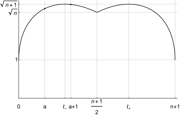
Figure 6: The graph of $\psi(t)$ for $n=5$. Here $n+1=5$, $a=1$, $t_{-}=(6-\sqrt{6})/2$

The graph of the function $\psi(t)$ for $n=5$ is given in Fig.6. In this case $n+1=5$, $a=1$, and $t_{-}=(6-\sqrt{6})/2$.

Obviously, $\theta_{n}(B)\leq||P||_{B}\leq\sqrt{n+1}$. Combining these inequalities with the inequality $\theta_{n}(B_{n})\geq c\sqrt{n}$ (see (6.19)), we obtain the exact order of the value of $\theta_{n}(B_{n})$ related to dimension $n$, namely, $\theta_{n}(B_{n})\asymp\sqrt{n}.$

Another corollary of Theorem 7.1 provides the following sharp values of $\theta_{n}(B_{n})$ for $1\leq n\leq 4$:

$$\theta_{1}(B_{1})=1,\quad\theta_{2}(B_{2})=\frac{5}{3},\quad\theta_{3}(B_{3})=2,\quad\theta_{4}(B_{4})=\frac{11}{5}.$$ (7.11)

Of course, $\theta_{1}(B_{1})=1$, but this case also fits into the general scheme. For proving, let us calculate the norm of the projector corresponding to a regular simplex inscribed into $B_{n}$. By Theorem 7.1,

$$\|P\|_{B_{1}}=1,\quad\|P\|_{B_{2}}=\frac{5}{3},\quad\|P\|_{B_{3}}=2,\quad\|P\|_{B_{4}}=\frac{11}{5}.$$

Note that for each $n=1,2,3,4,$ we have

$$\|P\|_{B_{n}}=3-\frac{4}{n+1}.$$

But $\theta_{n}(B_{n})\geq 3-4/(n+1)$ for every positive integer $n$ so that, if $1\leq n\leq 4$, then

$$\theta_{n}(B_{n})=3-\frac{4}{n+1}.$$ (7.12)

This is equivalent to (7.11). If (7.12) is true, then any projector having minimum norm corresponds to a regular simplex inscribed into $B_{n}$. Really, thanks to (1.7), for any projector $P$ and the simplex $S=S_{P}$

$$\frac{n+1}{2}\Bigl{(}\|P\|_{B_{n}}-1\Bigr{)}+1\geq\xi(B_{n};S)\geq\xi_{n}(B_{n})=n,$$

i. e.,

$$\|P\|_{B_{n}}\geq 3-\frac{4}{n+1}.$$

If for some projector we have here an equality, then equalities take place in the above chain too. In this case, the corresponding simplex satisfies $\xi(B_{n};S)=\xi_{n}(B_{n})=n.$ This way $S$ is a regular simplex inscribed in the boundary sphere (see Section 3). Remark that the same approach provides the exact values of $\theta_{n}(Q_{n})$ for dimensions $n=1,2,3,7.$

Let us define an integer $k=k_{n}$ equal to that of the numbers $a$ or $a+1$, for which $\psi(t)$ takes a larger value. As it shown in [40], if $k=1$, then in $B_{n}$ there exists an $1$-point with respect to the simplex corresponding to $P$. For such $n$,

$$\xi(B_{n};S)=\frac{n+1}{2}\Bigl{(}\|P\|_{B_{n}}-1\Bigr{)}+1$$ (7.13)

(see (1.7)). Since $S$ is a regular simplex inscribed into $B_{n}$, then $\xi(B_{n};S)=n$ and (7.13) is equivalent to the equality $\|P\|_{B_{n}}=3-\frac{4}{n+1}$. However, $k>1$ provided $n\geq 5$. This corresponds to the fact that (7.12) and (7.13) hold only for $1\leq n\leq 4$. Initially, this effect was discovered in the course of computer experiments perfomed by Alexey Ukhalov. Later the author gave an analytical solution to this problem. See [40] for details.

Numbers $k_{n}$ increase with $n$, but not strictly monotonously. For example,

$$k_{1}=k_{2}=k_{3}=k_{4}=1,\quad k_{5}=k_{6}=2,\quad k_{7}=k_{8}=k_{9}=3,\quad k_{10}=k_{11}=4,$$

$$k_{12}=k_{13}=5,\quad k_{14}=k_{15}=6,\quad k_{50}=22,\quad k_{100}=45,\quad k_{1000}=485.$$

Furthermore, $k_{n}\leq n/2$ provided $n\geq 2$.

8. A theorem on a simplex and its minimal ellipsoid

In 1948, F. John [11] proved that any convex body in ${\mathbb{R}}^{n}$ contains a unique ellipsoid of the maximum volume. Also he gave a characterization of those convex bodies for which the maximal ellipsoid is the unit Euclidean ball $B_{n}$ (see, e.g., [2], [3] for details). John’s theorem implies the analogous statement which characterizes a unique minimum volume ellipsoid containing a given convex body.

We shall consider the minimum volume ellipsoid containing a given nondegenerate simplex. For brevity, such an ellipsoid will be called the minimal ellipsoid. Obviously, the minimal ellipsoid of a simplex is circumscribed around this simplex. The center of the ellipsoid coincides with the center of gravity of the simplex. The minimal ellipsoid of a simplex is a Euclidean ball if and only if this simplex is regular. This is equivalent to the well-known fact that the volume of a simplex contained in a ball is maximal iff this simplex is regular and inscribed into the ball (see, e. g., [5], [51], [55]).

Let $S$ be a nondegenerate $n$-dimensional simplex in ${\mathbb{R}}^{n}$ and let $E$ be the minimum volume ellipsoid containing $S$. Let $m$, $1\leq m\leq n$, be a positive integer. To any $m$-point set of vertices of $S$, let us assign a point $y\in E$ defined as follows. Let $g$ be the center of gravity of the $(m-1)$-dimensional face of $S$ which contains the chosen vertices, and let $h$ be the center of gravity of the $(n-m)$-dimensional face which contains the rest $n+1-m$ vertices. Then $y$ is the intersection point of the straight line $(gh)$ with the boundary of the ellipsoid in direction from $g$ to $h$.

Theorem 8.1. ([32]) For every nondegenerate simplex $S\subset B_{n}$, there exists such a set of $m$ vertices for which $y\in B_{n}$.

Proof. Let $x^{(j)}$, $j=1,...,n+1$, be the vertices of $S$. The center of gravity of the simplex and also the center of gravity of its minimal ellipsoid $E$ are the point $c=({1}/({n+1}))\sum x^{(j)}.$ We let $r$ denote the ratio of the distance between the center of gravity of a regular simplex and the center of gravity of its $(m-1)$-dimensional face to the radius of the circumscribed sphere. It is easy to see that

$$r=\frac{1}{m}\sqrt{m-\frac{m(m-1)}{n}}.$$

Let $N$ be the number of $(m-1)$-dimensional faces of an $n$-dimensional simplex; thus, $N={n+1\choose m}$.

Let $J$ be an $m$-element subset of the set $\{1,...,n+1\}$. The center of gravity of the $(m-1)$-dimensional face with vertices $x^{(j)},j\in J,$ is the point $g_{J}=(1/m)\sum_{j\in J}x^{(j)}$. Suppose $y_{J}$ coincides with the point $y$ for this set of vertices. Then

$$y_{J}=c+\frac{1}{r}\left(c-g_{J}\right),$$

i.e., $y_{J}=(1/r)((r+1)c-g_{J})$. Summing up over all sets $J$, we have

$$\sum_{J}\|y_{J}\|^{2}=\sum_{J}\langle y_{J},y_{J}\rangle=$$

$$=\frac{1}{r^{2}}\left(N\|c\|^{2}(r+1)^{2}+\sum_{J}\|g_{J}\|^{2}-2(r+1)\langle\sum_{J}g_{J},c\rangle\right)=$$

$$=\frac{1}{r^{2}}\left(N\|c\|^{2}(r^{2}-1)+\sum_{J}\|g_{J}\|^{2}\right).$$ (8.1)

We took into account the equality $\sum g_{J}=Nc.$ Further, we claim that

$$\sum_{J}\|g_{J}\|^{2}=\frac{1}{mn}{n\choose m}\sum_{j=1}^{n+1}\|x^{(j)}\|^{2}+\frac{(m-1)(n+1)}{mn}{n+1\choose m}\|c\|^{2}.$$ (8.2)

To obtain (8.2), let us remark the following. The value $\sum\|g_{J}\|^{2}$ contains, for every $j$, exactly ${n\choose m-1}$ numbers $\|x^{(j)}\|^{2}$ taken with coefficient $1/m^{2}$, and exactly ${n-1\choose m-2}$ numbers $2\langle x^{(i)},x^{(j)}\rangle$, for each $i\neq j$, with the same coefficient $1/m^{2}$. (The latter ones exist for $m\geq 2$; in case $m=1$ there are no pairwise products.) The expression $\|c\|^{2}$ contains all numbers $\|x^{(j)}\|^{2}$, for any $j$, and numbers $2\langle x^{(i)},x^{(j)}\rangle$, for $i\neq j$, with multiplier $1/(n+1)^{2}.$ The coefficient at $\|c\|^{2}$ in the right-hand part of (8.2) guarantees the equality of expressions with pairwise products $\langle x^{(i)},x^{(j)}\rangle$; the coefficient at $\sum\|x^{(j)}\|^{2}$ is chosen so that the difference of the left-hand part of (8.2) and the second item in the right-hand part is equal to the first item. Since

$$N(r^{2}-1)=-\frac{(m-1)(n+1)}{mn}{n+1\choose m},$$

after replacing $\sum\|g_{J}\|^{2}$ in (8.1) with the right-hand part of (8.2), we notice that items with $\|c\|^{2}$ are compensated. After these transformations, we get

$$\frac{1}{N}\sum_{J}\|y_{J}\|^{2}=\frac{1}{n+1}\sum_{j=1}^{n+1}\|x^{(j)}\|^{2}.$$ (8.3)

The inclusion $S\subset B_{n}$ means that $\|x^{(j)}\|\leq 1.$ Therefore, the mean value of numbers $\|y_{J}\|^{2}$ is also $\leq 1.$ Consequently, for some set $J$ we have $\|y_{J}\|\leq 1,$ i.e., this point $y_{J}$ lies in $B_{n}.$ Theorem 8.1 is proved. $\Box$

The approach using in this proof was suggested and kindly communicated to the author by Arseniy Akopyan.

As a conjecture, Theorem 8.1 was formulated by the author in [30] . Also in [30], the statement of the theorem for $m=1$ was proved in a simpler way. In the case $m=1$ the points $y$ have the form $y^{(j)}=2c-x^{(j)},$ $j=1,\ldots,n+1,$ where $x^{(j)}\in B_{n}$ are the vertices of $S$ and $c=c(S)=c(E).$ We need to show that there exists a vertex $x$ of the simplex such that $\|2c-x\|\leq 1$. Since simplex $S$ is nondegenerate, for some vertex $x$ holds $\langle c,x-c\rangle\geq 0$. This implies

$$\|2c-x\|^{2}=\langle 2c-x,2c-x\rangle=4\langle c,c-x\rangle+\|x\|^{2}\leq\|x\|^{2}\leq 1,$$

i.e., the vertex $x$ is suitable.

9. The value of $\theta_{n}(B_{n})$

In this section we present the main result of the work [32] devoted to calculation of the exact value of the constant $\theta_{n}(B_{n})$.

Theorem 9.1. Let $\psi$ and $a_{n}$ be the function and the number defined by the equalities (7.3) and (7.4) respectively. Then, for every $n\in{\mathbb{N}}$ the following equality

$$\theta_{n}(B_{n})=\max\{\psi(a_{n}),\psi(a_{n}+1)\}$$ (9.1)

holds. Furthermore, an interpolation projector $P:C(B_{n})\to\Pi_{1}({\mathbb{R}}^{n})$ satisfies the equality $\|P\|_{B_{n}}=\theta_{n}(B_{n})$ if and only if its interpolation nodes coincide with the vertices of a regular simplex inscribed into the boundary sphere.

Proof. First, let $P$ be an interpolation projector corresponding to a regular inscribed simplex $S$, and let $\lambda_{j}(x)$ be the basic Lagrange polynomials for this simplex. Let $p_{n}=\|P\|_{B_{n}}$. Theorem 7.1 tells us that $p_{n}=\max\{\psi(a_{n}),\psi(a_{n}+1)\}.$ The points $y\in B_{n}$ satisfying

$$\sum_{j=1}^{n+1}|\lambda_{j}(y)|=p_{n}$$ (9.2)

were found in [30]. Namely, assume $k_{n}$ coincides with that of the numbers $a_{n}$ and $a_{n}+1$ which delivers to $\psi(t)$ the maximum value. Let us fix $m=k_{n}$. Then (9.2) takes place for every point $y$ which is constructed as in Theorem 8.1 in case $E=B_{n}$. The number of these points $y$ is $N={n+1\choose m}$.

Now, let $P:C(B_{n})\to\Pi_{1}({\mathbb{R}}^{n})$ be an arbitrary projector with the nodes $x^{(j)}\in B_{n}$, $S$ be the simplex with the vertices $x^{(j)}$, and $E$ be the minimum volume ellipsoid contained $S$. We can also consider $P$ as a projector acting from $C(E)$. By arguments related to affine equivalence, the norm $\|P\|_{E}$ coincides with the $(C(B_{n})$-$C(B_{n}))$-norm of a projector corresponding to a regular simplex inscribed into $B_{n}$, i.e., $\|P\|_{E}=p_{n}.$ Moreover,

$$\|P\|_{E}=\sum_{j=1}^{n+1}|\lambda_{j}(y)|$$

for $m=k_{n}$ and for each of the points $y$ noted at the beginning of the previous section (now with respect to the minimal ellipsoid $E$).

Theorem 8.1 tells us that at least one of these points, say $y^{*}$, belongs to $B_{n}$. Therefore,

$$\|P\|_{B_{n}}=\max_{x\in B_{n}}\sum_{j=1}^{n+1}|\lambda_{j}(x)|\geq\sum_{j=1}^{n+1}|\lambda_{j}(y^{*})|=\|P\|_{E}=p_{n}.$$

Thus, $\theta_{n}(B_{n})=p_{n}=\max\{\psi(a_{n}),\psi(a_{n}+1)\}=\psi(k_{n})$.

Let us show that if $\|P\|_{B_{n}}=\theta_{n}(B_{n})$, then the simplex with vertices at the interpolation nodes is inscribed into $B_{n}$ and regular. For this simplex $S$, some point $y\in E$, constructed for $m=k_{n}$, falls on the boundary sphere; otherwise we have $\|P\|_{B_{n}}>p_{n}=\theta_{n}(B_{n})$. This is due to the fact that $\sum|\lambda_{j}(x)|$ increases monotonously as $x$ moves in a straight line in direction from $c$ to $y$.

Since $\|y\|=1,$ the mean value of $\|y_{J}\|$ for the rest $y_{J}$ is also $\leq 1$ (see (8.3)). Hence, another such point also lies in the boundary of the ball. Thus we obtain $\|y_{J}\|=1$ for all sets $J$ consisting of $m=k_{n}$ indices $j$. Now (8.3) yields $\|x^{(j)}\|=1,$ i.e., the simplex is inscribed into the ball. Since all the points $y_{J}$ belong to the boundary sphere, the function $\sum|\lambda_{j}(x)|$ has maximum upon the ball at $N={n+1\choose m}$ different points. Consequently, the simplex $S$ is regular, and the proof of the theorem is complete. $\Box$

For $1\leq n\leq 4$, equality (9.1) and characterization of minimal projectors were obtained in [40] and [30] by another methods.

Corollary 9.1. For every $n\in{\mathbb{N}}$, the following inequalities

$$\sqrt{n}\leq\theta_{n}(B_{n})\leq\sqrt{n+1}$$

hold. Moreover, $\theta_{n}(B_{n})=\sqrt{n}$ only for $n=1$ and $\theta_{n}(B_{n})=\sqrt{n+1}$ if and only if $\sqrt{n+1}$ is an integer.

In fact, it was proved in [40] that the above relations are satisfied for $p_{n}=\max\{\psi(a_{n}),\psi(a_{n}+1)\}$. Combining this property with the result of Theorem 9.1, we obtain Corollary 9.1.

10. Interpolation by wider polynomial spaces

Let us briefly demonstrate how some of the above methods can be applied to interpolation by wider polynomial spaces. This approach has been realized in [18], [19] and in details described in [24].

Let $\Omega$ be a closed bounded subset of ${\mathbb{R}}^{n}$. Let $d\geq n+1,$ and let $\{\varphi_{1}(x),\ldots,\varphi_{d}(x)\}$ be a family of pairwise different monomials $x^{\alpha}=x_{1}^{\alpha_{1}}\ldots x_{n}^{\alpha_{n}}.$ Here $x=(x_{1},\ldots,x_{n})\in{\mathbb{R}}^{n}$, $\alpha=(\alpha_{1},\ldots,\alpha_{n})$ $\in{\mathbb{Z}}_{+}^{n}$. We suppose that $\varphi_{1}(x)\equiv 1,$ $\varphi_{2}(x)=x_{1},\ \ldots,\ \varphi_{n+1}(x)=x_{n}.$

By the $d$-dimensional space of polynomials in $n$ variables we mean the set $\Pi={\rm lin}(\varphi_{1},\ldots,\varphi_{d})$, i.e., the linear span of the family $\{\varphi_{1}(x),\ldots,\varphi_{d}(x)\}$. Let us note the following important cases: $\Pi=\Pi_{k}\left({\mathbb{R}}^{n}\right)$ – the space of polynomials of degree at most $k$  $(k\in{\mathbb{N}})$, and $\Pi=\Pi_{\alpha}\left({\mathbb{R}}^{n}\right)$ – the space of polynomials of degree $\leq\alpha_{i}$ in $x_{i}$   $(\alpha\in{\mathbb{N}}^{n}).$

A collection of points $x^{(1)},\ldots,x^{(d)}\in\Omega$ is called an admissible set of nodes for interpolation of functions from $C(\Omega)$ with the use of polynomials from $\Pi$ provided $\det({\bf A})\neq 0.$ This time $\bf A$ is $(d\times d)$-matrix

$${\bf A}=\left(\begin{array}[]{cccc}1&\varphi_{2}\left(x^{(1)}\right)&\ldots&\varphi_{d}\left(x^{(1)}\right)\\ \vdots&\vdots&\vdots&\vdots\\ 1&\varphi_{2}\left(x^{(d)}\right)&\ldots&\varphi_{d}\left(x^{(d)}\right)\end{array}\right).$$

Assume that $\Omega$ contains such a set of nodes. For the interpolation projector $P:C(\Omega)\to\Pi$ with these nodes, we have

$$Pf(x)=\sum_{j=1}^{d}f\left(x^{(j)}\right)\lambda_{j}(x),\quad\|P\|_{\Omega}=\max\limits_{x\in\Omega}\sum_{j=1}^{d}|\lambda_{j}(x)|.$$ (10.1)

Here $\lambda_{j}\in\Pi$ are the polynomials having the property $\lambda_{j}\left(x^{(k)}\right)$ $=$ $\delta_{j}^{k}.$ Their coefficients with respect to the basis $\varphi_{1},$ $\ldots,$ $\varphi_{d}$ form the columns of ${\bf A}^{-1}.$

Let us introduce the mapping $T:{\mathbb{R}}^{n}\to{\mathbb{R}}^{d-1}$ defined in the way

$$y=T(x)=(\varphi_{2}(x),\ldots,\varphi_{d}(x))=(x_{1},\ldots,x_{n},\varphi_{n+1}(x),\ldots,\varphi_{d}(x)).$$

We will consider $T$ on the set $\Omega.$ The choice of the first monomials $\varphi_{j}(x)$ implies the invertibility of $T.$ Let $y^{(j)}=T\left(x^{(j)}\right)$. Then the numbers $\lambda_{j}(x)$ are the barycentric coordinates of the point $y=T(x)$ with respect to the $(d-1)$-dimensional simplex with vertices $y^{(j)}$.

We set

$$\theta(\Pi;\Omega)=\min\limits_{x^{(j)}\in\Omega}\|P\|_{\Omega},$$

and

$$\xi_{n}(\Omega)=\min\left\{\xi(\Omega;S):\,S~{}\mbox{is an $n$-dimensional simplex,}\,{\rm ver}(S)\subset\Omega,\,{\rm vol}(S)\neq 0\right\}.$$

The value $\xi(\Omega;S)$ is defined as for a convex $\Omega$.

If $x^{(1)},\ldots,x^{(d)}\in\Omega$ is an admissible set of nodes to interpolate functions from $C(\Omega)$ by polynomials from $\Pi$, then $y^{(j)}=T\left(x^{(j)}\right)$ is an admissible set of nodes to interpolate functions from $C(T(\Omega))$ by polynomials from $\Pi_{1}\left({\mathbb{R}}^{d-1}\right).$ For the projector $\overline{P}:C(T(\Omega))\to\Pi_{1}\left({\mathbb{R}}^{d-1}\right)$ with the nodes $y^{(1)},\ldots,y^{(d)},$ we have $\|\overline{P}\|_{T(\Omega)}=\|P\|_{\Omega}.$ By this, when estimating the norm $\|P\|_{\Omega}$, it turns out to be possible to apply geometric inequalities for the norm of projector $\overline{P}$ under linear interpolation on the $(d-1)$ dimensional set $T(\Omega)$. Thus we obtain estimates of the norms $\|P\|_{\Omega}$ through the absorption coefficients $\xi(T(\Omega);S)$ or through the function $\chi_{d-1}^{-1}$ (modifications of (6.22) for $K={\rm conv}(T(\Omega))$) and some others.

For the projector $P:C(\Omega)\to\Pi$ with nodes $x^{(j)}$, we have

$$\frac{1}{2}\left(1+\frac{1}{d-1}\right)\left(\|P\|_{\Omega}-1\right)+1\leq\xi(T(\Omega);S)\leq\frac{d}{2}\left(\|P\|_{\Omega}-1\right)+1,$$ (10.2)

where $S$ is the $(d-1)$-dimensional simplex with the vertices $T\left(x^{(j)}\right).$ Also we obtain the following inequalities:

$$\frac{1}{2}\left(1+\frac{1}{d-1}\right)\left(\theta(\Pi;\Omega)-1\right)+1\leq\xi_{d-1}(T(\Omega))\leq\frac{d}{2}\left(\theta(\Pi;\Omega)-1\right)+1.$$ (10.3)

The right-hand inequality in (10.2) becomes an equality, when there exists a $1$-point $y=T(x)\in T(\Omega)$ with respect to the simplex $S={\rm conv}\left(y^{(1)},\ldots,y^{(d)}\right)$. This means that for the corresponding $x$ simultaneously $\|P\|_{\Omega}=\sum_{j=1}^{d}|\lambda_{j}(x)|$ and among the numbers $\lambda_{j}(x)$ there is the only one negative.

For the case $\Pi=\Pi_{1}\left({\mathbb{R}}^{n}\right)$ and $\Omega=Q_{n}$ or $B_{n}$ see the previous text. Some other examples are given in [24]. The simplest case of nonlinear interpolation is quadratic interpolation on a segment. An analytical solution of the minimal projector problem with the indicated geometric approach is given in [18] (see also [24] and [44]). Let us consider this case as an illustrative example.

It is well known (see, e. g., [47]) that the minimal norm of an interpolation projector is attained for regular nodes and equals ${5}/{4}$. We claim that this result can be also obtained with the use of inequalities (10.2) and (10.3). In addition, it turns out that there are infinitely many minimal projectors.

If $\Pi=\Pi_{2}\left({\mathbb{R}}^{1}\right)$, then $d=\dim\Pi=3,$ i.e., $k=d-1=2.$ The mapping $T$ has the form $x\longmapsto(x,x^{2})$ and the set $T(\Omega)=T([-1,1])=\{(x,x^{2})\in{\mathbb{R}}^{2}:\,-1\leq x\leq 1\}$ is a piece of parabola. For the interpolation nodes $-1\leq r<s<t\leq 1$ the simplex $S$ is the triangle with the vertices $(r,r^{2}),\,(s,s^{2}),\,(t,t^{2})$ lying on this part of parabola. The absorption of the parabolic sector by this triangle is shown in Fig. 7 .

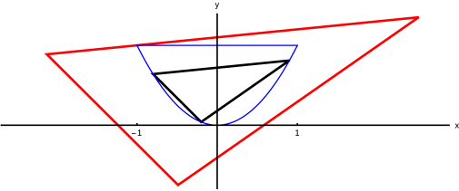
Figure 7: The absorption of the parabolic sector by a triangle

The convexity of the function $\psi(x)=x^{2}$ implies that a $1$-point of the set $T([-1,1])$ with respect to $S$ exists for any nodes. Hence, we have an equality in the right-hand part of (10.2):

$$\xi(T(\Omega);S)=\frac{3}{2}\left(\|P\|_{\Omega}-1\right)+1=\frac{3\|P\|_{\Omega}-1}{2}.$$ (10.4)

Since (10.4) holds for an arbitrary projector $P:C[-1,1]\to\Pi_{2}({\mathbb{R}}^{1})$, we have the right-hand equality also in (10.3):

$$\xi_{2}(T(\Omega))=\frac{3\theta\left(\Pi;\Omega\right)-1}{2}.$$

So, finding the minimum norm of a projector $\theta\left(\Pi;\Omega\right)$ is equivalent to calculating $\xi_{2}(T(\Omega))$. This problem is reducible to a triangle $S$ with vertices $(-r,r^{2}),$ $(0,0),$ $(r,r^{2}),$ $0<r\leq 1.$ For this triangle,

$$\xi(T(\Omega);S)=\max\left(\frac{11}{8},\frac{3}{r^{2}}-2\right),\quad\|P\|_{\Omega}=\max\left(\frac{5}{4},\frac{2}{r^{2}}-1\right).$$

If $2\sqrt{2}/3=0.9428\ldots\leq r\leq 1,$ then these values do not depend on $r$ and are equal correspondingly to $11/8$ and  $5/4$ ; these are the minimal possible values. Thus,

$$\xi_{2}(T(\Omega))=\frac{11}{8}~{}~{}~{}\text{and}~{}~{}~{}\theta\left(\Pi;\Omega\right)=\frac{5}{4}.$$

The minimal is an arbitrary projector with vertices $-r,$ $0,$ $r$ where $r\in\left[\frac{2\sqrt{2}}{3},1\right]$. There are no other minimal projectors.

In [44], we give estimates of $\theta\left(\Pi_{k}\left({\mathbb{R}}^{1}\right);[-1,1]\right)$ and $\xi_{k}\left(T([-1,1])\right)$ for $1\leq k\leq 10$. In this paper we have studied the fulfillment of equality in the right-hand side of (10.2) for simplices delivering the found upper bounds of $\xi_{k}\left(T([-1,1])\right)$ and also for uniform and Chebyshev nodes.

This work is intended to be continued in the multidimensional case.

Acknowledgements

I am very thankful to Pavel Shvartsman for useful suggestions and remarks.

References

[1]
[2]K. Ball.
Ellipsoids of maximal volume in convex bodies,
arXiv: math/9201217v1
[3]K. Ball.An Elementary Introduction to Modern Convex Geometry,Math. Sci. Res. Inst. Publ., 31:1 (1997), 1–58.
[4]Clements G. F., Lindström B. A sequence of
determinants with large values, Proc. Amer. Math. Soc., 16 (1965), 548–550.
[5]L. Fejes Tót.Regular Figures, New York: Macmillan/Pergamon, 1964.
[6]G. M. Fikhtengol’ts.The Course in Differential and Integral Calculation. Vol.3, Fizmatlit, Moscow, 2001 (in Russian).
[7]K. J. Horadam.Hadamard Matrices and Their Applications, Princeton University Press, 2007.
[8]J. Hadamard. Résolution d’une question relative aux déterminants,
Bull. Sciences Math. (2),17 (1893), 240–246.
[10]M. Hudelson, V. Klee, and D. Larman. Largest -simplices
in -cubes: some relatives of the Hadamard maximum determinant
problem, Linear Algebra Appl., 241–243 (2019), 519–598.
[11]F. John.
Extremum Problems with Inequalities as Subsidiary Conditions,
in: Studies and essays presented to R. Courant on his 60th birthday (Jan. 8, 1948), New York: Interscience, 1948, 187–204.
[12]M. S. Klamkin and G. A. Tsifinis.
Circumradius-inradius inequality for a simplex, Mathematics Magazine,52:1 (1979), 20–22.
[13]M. Lassak. Parallelotopes of maximum volume in a simplex,
Beitr. Algebra Geom.,52 (2011), 389–394.
[14]M. Lassak. Approximation of convex bodies by inscribed simplices of maximum volume,
Discr. Comput. Geom.,21 (1999), 449–462.
[15]P. K. Manjhi and M. K. Rama. Some new examples of circulant partial Hadamard matrices of type ,
Advances and Applications in Mathematical Sciences,21:5 (2022), 2559–2564.
[16]M. V. Nevskii. Estimates for the minimum norm of a projection in linear interpolation over the vertices of an
-dimensional cube, Model. Anal. Inform. Sist.,10:1 (2003), 9–19 (in Russian).
[17]M. V. Nevskii. Geometric methods in the minimal projection problem,
Model. Anal. Inform. Sist.,13:2 (2006), 16–29
(in Russian).
[18]M. V. Nevskii. Inequalities for the norms of interpolating projections,
Model. Anal. Inform. Sist.,15:3 (2008), 28–37
(in Russian).
[19]M. V. Nevskii. On a certain relation for the minimal norm of an interpolational projection,
Model. Anal. Inform. Sist.,16:1 (2009), 24–43
(in Russian).
[20]
M. V. Nevskii, On a property of -dimensional simplices, Mat. Zametki,87:4 (2010), 580–593
(in Russian). English translation: Math. Notes,87:4 (2010), 543–555.
[21]M. V. Nevskii. On geometric characteristics of an -dimensional simplex,
Model. Anal. Inform. Sist.,18:2 (2011), 52–64
(in Russian).
[22]M. Nevskii. Properties of axial diameters of a simplex,
Discr. Comput. Geom.,46:2 (2011), 301–312.
[23]M. V. Nevskii. On the axial diameters of a convex body, Mat. Zametki,90:2 (2011), 313–315
(in Russian). English translation: Math. Notes,90:2 (2011), 295–298.
[24]M. V. Nevskii.Geometric Estimates in Polynomial
Interpolation, P. G. Demidov Yaroslavl’ State University, Yaroslavl’, 2012 (in Russian).
[25]M. V. Nevskii. On the minimal positive homothetic image of a simplex which contains
a convex body, Mat. Zametki,93:3 (2013), 295–298
(in Russian). English translation: Math. Notes,93:3–4 (2011), 470–478.
[26]M. V. Nevskii. On some problem for a simplex and a cube in ,
Model. Anal. Inform. Sist.,20:3 (2013), 77–85
(in Russian). English translation: Aut. Control Comp. Sci.,48:7 (2014), 521–527.
[27]M. V. Nevskii. Computation of the longest segment of a given direction in a simplex,
Fundam. Prikl. Mat., 18:2 (2013), 147–152
(in Russian).
English translation: J.
Math. Sci., 203:6 (2014), 851–854.
[28]M. V. Nevskii. On some problems for a simplex and a ball in ,
Model. Anal. Inform. Sist., 25:6 (2018), 680–691
(in Russian).
English translation: Aut.
Control Comp. Sci., 53:7 (2019), 644–652.
[29]M. V. Nevskii. Geometric estimates in interpolation on an n-dimensional ball,
Model. Anal. Inform. Sist., 26:3 (2019), 441–449
(in Russian).
English translation: Aut.
Control Comp. Sci., 54:7 (2020), 712–718.
[30]M. V. Nevskii. On properties of a regular simplex inscribed into a ball,
Model. Anal. Inform. Sist., 28:2 (2021), 186–197
(in Russian).
English translation: Aut.
Control Comp. Sci., 56:7 (2022), 778–787.
[31]M. V. Nevskij. On some estimate for the norm of an interpolation projector, Model. Anal. Inform. Sist.,29:2 (2022), 92–103 (in Russian). English translation: Aut. Control Comp. Sci.,57:7 (2023), 718–726.
[32]M. V. Nevskii. On the minimal norm of the projection operator for linear interpolation
on an -dimensional ball, Mat. Zametki,114:3 (2023), 477–480
(in Russian). English translation: Math. Notes,114:3 (2023), 415–418.
[33]M. V. Nevskii and A. Yu. Ukhalov. On numerical characteristics of a simplex and their estimates,
Model. Anal. Inform. Sist., 23:5 (2016), 602–618
(in Russian).
English translation: Aut.
Control Comp. Sci., 51:7 (2017), 757–769.
[34]M. V. Nevskii and A. Yu. Ukhalov. New estimates of numerical values related to a simplex,
Model. Anal. Inform. Sist., 24:1 (2017), 94–110
(in Russian).
English translation: Aut.
Control Comp. Sci., 51:7 (2017), 770–782.
[35]M. V. Nevskii and A. Yu. Ukhalov. On -dimensional simplices satisfying inclusions ,
Model. Anal. Inform. Sist., 24:5 (2017), 578–595
(in Russian).
English translation: Aut.
Control Comp. Sci., 52:7 (2018), 667–679.
[36]M. V. Nevskii and A. Yu. Ukhalov. On minimal absorption index for an -dimensional simplex,
Model. Anal. Inform. Sist., 25:1 (2018), 140–150
(in Russian).
English translation: Aut.
Control Comp. Sci., 52:7 (2018), 680–687.
[37]M. Nevskii and A. Ukhalov. Perfect Simplices in ,
Beitr. Algebra Geom.,59:3 (2018), 501–521.
[38]M. V. Nevskii and A. Yu. Ukhalov.
On optimal interpolation by linear functions on an -dimensional cube,
Model. Anal. Inform. Sist., 25:3 (2018), 291–311
(in Russian).
English translation: Aut.
Control Comp. Sci., 52:7 (2018), 828–842.
[39]M. V. Nevskii and A. Yu. Ukhalov.
Some properties of -simplices, Izv. Saratov Univ.
(N. S.), Ser. Math. Mech. Inform.,18:3 (2018), 305–315 (in Russian).
[40]M. V. Nevskii and A. Yu. Ukhalov.
Linear interpolation on a Euclidean ball in ,
Model. Anal. Inform. Sist., 26:2 (2019), 279–296
(in Russian).
English translation: Aut.
Control Comp. Sci., 54:7 (2020), 601–614.
[41]M. Nevskii and A. Ukhalov.
Properties of -matrices of order having maximal determinant, Matem. zametki SVFU,26:2 (2019), 109–115 (in Russian).
[42]M. Nevskii and A. Ukhalov. Functions for checking necessary conditions for maximality of 0/1-determinant and example // doi: 10.17632/sm3x4xrb42.1 url: http://dx.doi.org/10.17632/sm3x4xrb42.1
Complementary materials to the paper: M. Nevskii and A. Ukhalov, Properties of -matrices of order n having maximal determinant, Math. Notes of NEFU,26:2 (2019), 109–115.
[43]M. V. Nevskii and A. Yu. Ukhalov. Estimates for norms of interpolation projectors and related problems in computational geometry, In: Mathematics at Yaroslavl University:
Collection of Review Articles: To the 45th Anniversary of the Department of Mathematics,
P. G. Demidov Yaroslavl’ State University, Yaroslavl’, 2021, 182–231 (in Russian).
English translation: arXiv:2108.00880v1
[44]M. V. Nevskii and A. Yu. Ukhalov. On a geometric approach to the estimation of
interpolation projectors,
Model. Anal. Inform. Sist., 30:3 (2023), 246–257
(in Russian). English translation: arXiv:2307.13780v1
[45]M. V. Nevskii and A. Yu. Ukhalov.Selected Problems in Analysis and Computational Geometry. Part 1,
P. G. Demidov Yaroslavl’ State University, Yaroslavl’, 2020 (in Russian).
[46]M. V. Nevskii and A. Yu. Ukhalov.Selected Problems in Analysis and Computational Geometry. Part 2,
P. G. Demidov Yaroslavl’ State University, Yaroslavl’, 2022 (in Russian).
[47]S. Pashkovskij.Vychislitel’nye Primeneniya Mnogochlenov i Ryadov Chebysheva, Nauka, Moskva, 1983 (in Russian).
[48]A. P. Prudnikov, Yu. A. Brychkov, O. I. Marichev.Integraly i Ryady, Nauka, Moskva, 1981
(in Russian).
[49]P. R.Scott.
Lattices and convex sets in space, Quart. J. Math. Oxford Ser. (2),36 (1985), 359–362.
[51]D. Slepian.
The content of some extreme simplices,
Pacific J. Math.,31 (1969), 795–808.
[52]P. K. Suetin.Klassicheskie ortogonal’nye mnogochleny, Nauka, Moskva,1979 (in Russian).
[53]G. Szegö.Orthogonal Polynomials, American Mathematical Society, New York, 1959p.
[54]A. Ukhalov and E. Udovenko. Hadamard matrices of order 28 in machine readable form, Mendeley Data, V2, 2020.
doi: 10.17632/tw66ksdfhh.2.
https://data.mendeley.com/datasets/tw66ksdfhh/2
[55]D. Vandev.
A minimal volume ellipsoid around a simplex,
C. R. Acad. Bulg. Sci., 45:6 (1992), 37–40.
[56]A. Vince. A simplex contained in a sphere, J. Geom.,89:2 (2008), 169–178.
[57]S. Wolfram.Essentials of Programming in Mathematica, Cambridge University Press, 2016.
[58]S. Yang and J. Wang.
Improvements of -dimensional Euler inequality,
J. Geom.,51 (1994), 190–195.