Temporal Disentangled Contrastive Diffusion Model for Spatiotemporal Imputation

Abstract

Spatiotemporal data analysis is pivotal across various domains, including transportation, meteorology, and healthcare. However, the data collected in real-world scenarios often suffers incompleteness due to sensor malfunctions and network transmission errors. Spatiotemporal imputation endeavours to predict missing values by exploiting the inherent spatial and temporal dependencies present in the observed data. Traditional approaches, which rely on classical statistical and machine learning techniques, are often inadequate, particularly when the data fails to meet strict distributional assumptions. In contrast, recent deep learning-based methods, leveraging graph and recurrent neural networks, have demonstrated enhanced efficacy. Nonetheless, these approaches are prone to error accumulation. Generative models have been increasingly adopted to circumvent the reliance on potentially inaccurate historical imputed values for future predictions. These models grapple with the challenge of producing unstable results, a particular issue in diffusion-based models. We aim to address these challenges by designing conditional features to guide the generative process and expedite training. Specifically, we introduce C²TSD, a novel approach incorporating trend and seasonal information as conditional features and employing contrastive learning to improve model generalizability. The extensive experiments on three real-world datasets demonstrate the superior performance of C²TSD over various state-of-the-art baselines.

I Introduction

Multivariate time series data are widespread across various fields, such as economics, transportation, healthcare, and meteorology [1, 2, 3, 4]. Such data typically distinguish themselves from other data types in being spatiotemporal—they are chronologically ordered and often autocorrelated; they may exhibit recurring trends, patterns, or fluctuations; they may show stationarity or variability, etc. They serve as valuable assets in various domains and support mining actionable knowledge from those time series to make sense of the data [5]. Statistical and machine-learning techniques are traditionally applied to handle time series data, and they have proven effective in handling complete datasets in a multitude of time series tasks, including forecasting [6], classification [7], and anomaly detection [8]. Nevertheless, they face a practical challenge in real-world scenarios: time series data may contain missing values for various reasons, such as sensor malfunctions, packet loss in data transmission, poor management of data integrity, or even human neglect [9]. Those missing values could significantly compromise data quality, thus adversely affecting the performance of those methods in their respective tasks.

A range of statistical and machine-learning methods have been employed to estimate the missing values, e.g., autoregressive moving average (ARMA) [10], expectation-maximization (EM) [11], and $k$-nearest neighbors (kNN) [12]. These models, however, typically rely on strong assumptions about the temporal stationarity and inter-series similarity of the times series data to make estimations. Those assumptions do not necessarily capture the complexities of real-world multivariate time series data, leading to potentially unsatisfactory performance in practical scenarios.

Recent advances in deep learning have inspired new approaches to spatiotemporal imputation [13]. Notably, Recurrent Neural Network (RNN)-based methods [14] have drawn enormous attention in light of their proven effectiveness in handling time series data. Gated Recurrent Units (GRU) and bidirectional structures have shown advantages through recurrent updates of hidden states [9]. More recent efforts integrate Graph Neural Networks (GNNs) with RNNs to effectively learn spatial dependencies, a crucial aspect of spatiotemporal imputation [15]. Though promising, the above methods face the issue of error accumulation due to their recurrent structures [16], i.e., they heavily rely on previously estimated (and potentially inaccurate) historical values to infer further missing values, leading to deterministic outputs that fail to describe the inherent uncertainty of the imputation process.

Generative models have also shown significant performance in multivariate time series tasks [17]. For instance, SSGAN [18], a semi-supervised generative adversarial network (GAN), leverages observed information and data labels to guide the generator in estimating missing values. Among generative models, diffusion models stand out by offering a solution to the error accumulation problem [19]. Diffusion models typically initiate the prediction of missing values from randomly sampled Gaussian noise, transforming this noise into estimations of missing values. In general, diffusion models exhibit greater stability in training when compared with GAN-based models. For example, diffusion probabilistic models (DPMs) [20, 21], known for their impressive performance across various tasks, have been adapted for imputing multivariate time series data. Despite their capacity for high-quality content generation, these models generate the output by reversing the process of gradually introducing noise into the data, resulting in unpredictability in the final output. The output may thus misalign with specific user requirements or contextual demands from time to time. Recent efforts have introduced conditional information into diffusion models to address the above limitation [22, 23]. This directed generation approach is particularly advantageous in scenarios where outputs must adhere to certain themes, styles, or user-defined criteria. By integrating the conditional information, diffusion models can be fine-tuned to yield more predictable and relevant outcomes, enhancing their suitability for various practical applications.

We aim to design a comprehensive solution to spatiotemporal imputation by taking advantage of both diffusion models and structural time series models. Specifically, we introduce C²TSD in Fig. 1, a novel conditional diffusion framework that incorporates contrastive learning and trend-season disentanglement for effective spatiotemporal imputation. This framework is grounded in the principles of structural time series models [24], which disentangle time series as a combination of trend, seasonal, and error components. Disentangling trend and seasonal components, especially when enhanced with contrastive learning, has been demonstrated to be effective in time series forecasting [25]. Here, the disentanglement enables C²TSD to extract explainable temporal dependencies, thereby enhancing the learning of time series representations. Using distinct trend and seasonal representations as conditional inputs, our proposed model can direct the diffusion process toward generating easier-to-understand results, ensuring the reliability of the outcomes. Moreover, using a contrastive learning strategy significantly improves the model’s generalization on novel and unseen samples. Our experiments show the representational features developed through this learning approach exhibit enhanced robustness and representativeness, improving the model’s ability to handle noise and drift in our experimental datasets.

Our contributions are summarized as follows:

• We propose C²TSD, a Conditional diffusion framework for spatiotemporal imputation. Our framework integrates Contrastive learning with Trend-Season Disentanglement techniques to effectively capture the global spatiotemporal relationship.

• We introduce a trend-season disentanglement module to enhance the robustness of temporal relationship learning. This module can learn trend and seasonal dependencies separately to make the framework’s outputs easier to understand by users.

• We develop a contrastive learning strategy that aids in learning spatiotemporal dependencies and directs the generative process. This strategy contributes to the stability of the noise estimation module in our framework.

• Through extensive experiments on three real-world datasets from diverse fields (meteorology and transportation), C²TSD demonstrates superior performance in spatiotemporal imputation compared to multiple state-of-the-art baselines across various missing pattern scenarios.

The remainder of this paper is structured as follows. Section II provides a review of related work. In Section III, we elaborate our proposed model, focusing on the application of diffusion models to spatiotemporal imputation. Section IV reports an evaluation of our model across a range of missing data scenarios. Finally, we summarize our findings and contributions in Section V.

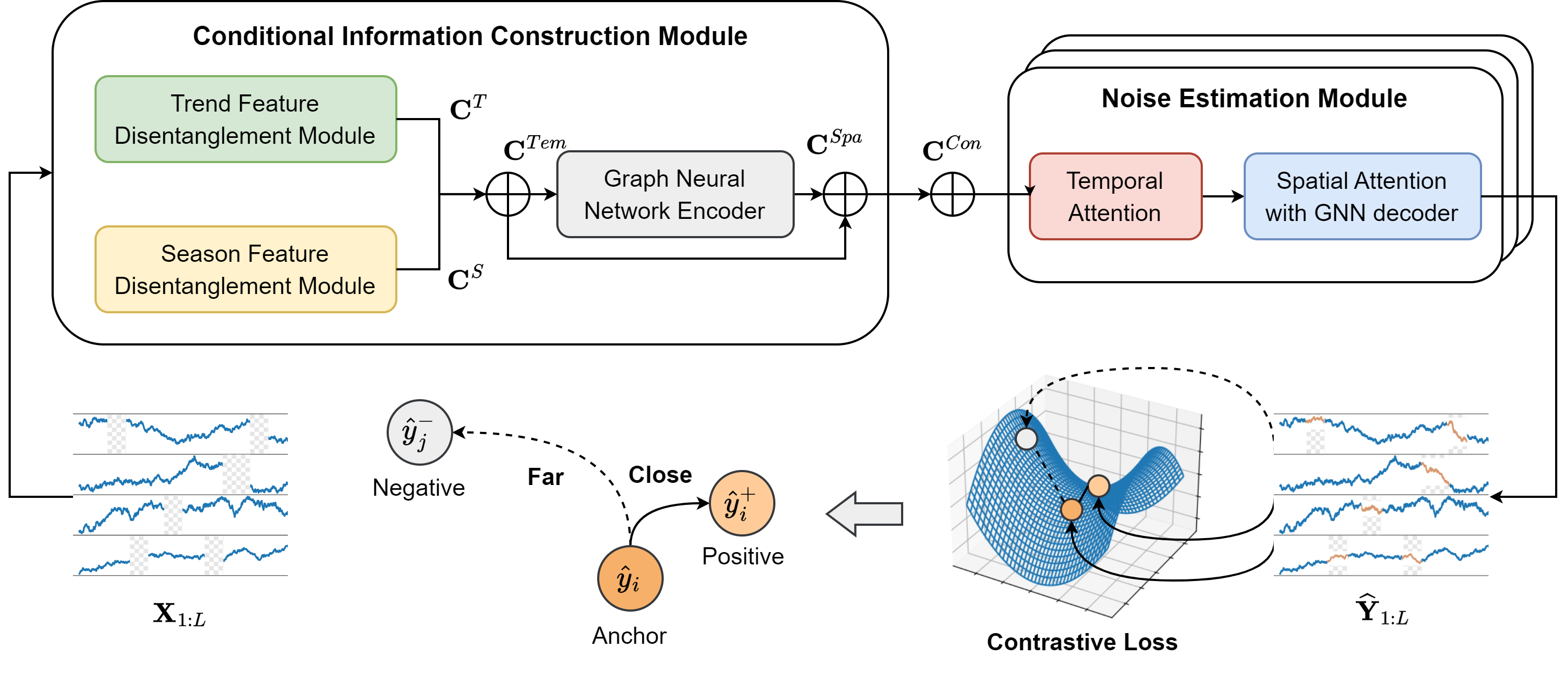
Figure 1: The architecture of our proposed model, C²TSD. The Conditional Information Construction Module (Section III-C1) processes input signals with missing values to generate conditional features $\mathbf{C}^{Con}$, which will later be used to guide the generative direction of the diffusion model. In parallel, the Noise Estimation Module (Section III-C2) utilizes the input, conditional features, and time embedding to accurately recover noise and attribute values in the output signals. Additionally, we have incorporated a contrastive learning strategy to redesign the loss function, further optimizing the model’s performance.

II Related Work

II-A Methods for Multivariate Time Series Imputation

Addressing missing values in multivariate time series analysis has been a significant challenge, leading to considerable research effort [26]. Traditional methods mainly include statistical and machine learning techniques such as ARMA [10], EM algorithms [11], and kNN [12]. However, these models often struggle with complex, non-stationary real-world data. Low-rank matrix factorization has also gained traction for spatiotemporal imputation, utilizing inherent spatial and temporal patterns. Key examples are TRMF [27], which integrates temporal regularized matrix factorization, and BATF [28], which applies augmented tensor factorization to transportation data. Another approach is TIDER [29], combining matrix factorization with time series disentanglement representation, enhancing spatiotemporal imputation.

Deep learning, particularly RNNs and GANs, has been increasingly used for multivariate time series imputation. GRU-D [9] employs GRU-based recurrent structures with masking and time interval integration, effectively capturing long-term temporal dynamics and missing patterns. BRITS [14] utilizes a bidirectional RNN to handle multiple correlated missing values and nonlinear time series dynamics, enhancing data-driven imputation. Through adversarial processes, GAN-based methods learn the entire data distribution and impute missing values, as shown in studies like [30, 31, 32]. Graph neural networks (GNNs) have also been applied, with STGNN-DAE [33] and GRIN [15] exploring spatial-temporal correlations using graph-based approaches. However, these methods often yield deterministic outputs, oversimplify complex dependencies, and show lower robustness to noisy or incomplete data. The deterministic nature of these models limits their adaptability to the inherent variability and uncertainty in real-world data.

II-B Diffusion Method in Multivariate Time Series

Diffusion models have been widely applied in multivariate time series tasks, including forecasting, imputation, and anomaly detection. TimeGrad [34], building on DDPM models [20], introduces noise at each predictive time point and uses a backward transition kernel conditioned on historical data for denoising. ScoreGrad [35] enhances TimeGrad by incorporating a conditional SDE-based score-matching module and using structures like temporal convolutional and attention-based networks for data encoding. D³VAE [36] employs a bidirectional auto-encoder to handle limited and noisy time series data. In forecasting, DiffSTG [37] combines diffusion models with UGnet, a graph-based method, to learn spatial-temporal relationships. For anomaly detection, D³R [38] uses data-time mix-attention in non-stationary environments to decompose long-period time series, while ImDiffusion [39] leverages neighboring time series values to model temporal and inter-correlated dependencies effectively.

Diffusion models have been increasingly employed to address the multivariate time series imputation problem, in light of their success in other time series tasks. CSDI [22] represents a seminal DDPM-based work in this domain. Another noteworthy contribution is SSSD [40], which has empirically demonstrated superior imputation outcomes using a structured state space model compared to other architectural approaches. SSSD uniquely targets the entire time series matrix for generation, deviating from traditional methods that focus on matrices representing missing values. PriSTI [23] introduced a noise-matching network comprising a conditional feature extraction and noise estimation modules. However, PriSTI primarily addresses imputation in single-feature spatiotemporal graphs (STGs), thus representing a specific subset of STGs. Nevertheless, existing methods have not emphasized the strategic design of conditional information to direct the generative process and enhance model stability, an aspect our work seeks to address.

III C²TSD

In this section, we initially describe the application of diffusion models to spatiotemporal imputation, followed by a detailed description of the various modules encompassed in our framework. The workflow of our framework, C²TSD, is illustrated in Fig. 1. C²TSD leverages a conditional diffusion framework using spatiotemporal correlations for effective imputation.

III-A Problem Statement

Spatiotemporal imputation involves predicting missing values in historical records. Let us represent the input training data as $\mathbf{X}_{1:L}={\mathbf{X}_{1},\ldots,\mathbf{X}_{l},\ldots,\mathbf{X}_{L}}$, where $\mathbf{X}_{l}={x^{1}_{l},x^{1}_{l},\ldots,x^{N}_{l}}$, with the superscript denoting series and the subscript indicating time. In contrast to forecasting tasks, all timestamps are available for training in imputation tasks. A mask matrix $\mathbf{M}\in{\{0,1\}}^{N\times l}$, corresponding in dimension to the input data, identifies the locations of missing values in the time series, where $m^{n}_{l}=0$ denotes a missing value at $x^{n}_{l}$, and $m^{n}_{l}=1$ otherwise. The output of the task, $\widehat{\mathbf{Y}}_{1:L}\in\mathbb{R}^{N\times L}$, matches the input in dimensions and is expected to contain all the previously missing values. Thus, the objective in multivariate time series imputation is to find values that most closely approximate the underlying ground truth, thereby effectively filling the missing gaps in $\mathbf{X}_{1:L}$.

III-B Diffusion Model for Spatiotemporal Imputation

Diffusion probabilistic models, a class of deep generative models, have gained competitive results in various domains, including object detection [41], text-to-image multi-modality [42], and recommendation systems [43]. These models generate samples consistent with the original data distribution by systematically introducing noise into the samples and subsequently learning the reverse denoising process. The diffusion model can be identified as two Markov Chain processes, each length $T$, known as the diffusion and reverse processes. Starting with $\widetilde{X}^{0}\sim p_{\mathit{data}}$, where $p_{\mathit{data}}$ denotes the original data distribution, $\widetilde{X}^{t}$ represents the sampled latent variable sequence for diffusion steps $t=1,\ldots,T$. At the final step, $\widetilde{X}^{T}$ approximates a Gaussian distribution, $\mathcal{N}(0,\mathbf{I})$. The diffusion process incrementally infuses Gaussian noise into $\widetilde{X}^{0}$ until it closely resembles $\widetilde{X}^{T}$, whereas the reverse process aims to denoise $\widetilde{X}^{t}$ to revert to $\widetilde{X}^{0}$.

To utilize diffusion models for spatiotemporal imputation, we conceptualize the spatiotemporal imputation task as a conditional generation problem. Prior studies [22, 23] have demonstrated the efficacy of conditional diffusion probabilistic models in this context. The essential task in spatiotemporal imputation involves estimating the conditional probability distribution $q(\widetilde{\mathbf{X}}^{0}_{1:L}|\mathbf{X}_{1:L})$, where the imputation of $\widetilde{\mathbf{X}}^{0}_{1:L}$ is contingent upon the observed values $\mathbf{X}_{1:L}$. This section demonstrates how our proposed framework employs diffusion models to impute spatiotemporal data. For the ensuing discussion, we use the superscript $t\in\{0,1,...,T\}$ to denote the diffusion steps and, for brevity, omit the subscripts $1:L$.

The diffusion model comprises two primary components: the diffusion and reverse processes. Specifically, the diffusion process in spatiotemporal imputation operates independently of conditional information. It involves the addition of Gaussian noise to the original data within the imputation target, a process that is formalized as follows:

$$\begin{split}q(\widetilde{\mathbf{X}}^{1:T}|\widetilde{\mathbf{X}}^{0})&=\prod_{t=1}^{T}q(\widetilde{\mathbf{X}}^{t}|\widetilde{\mathbf{X}}^{t-1})\\ q(\widetilde{\mathbf{X}}^{t}|\widetilde{\mathbf{X}}^{t-1})&=\mathcal{N}(\widetilde{\mathbf{X}}^{t};\sqrt{1-\beta_{t}}\widetilde{\mathbf{X}}^{t-1},\beta_{t}\mathbf{I})\end{split}$$ (1)

In the equation, $\beta_{t}$ denotes a small constant hyperparameter that determines the variance of the noise being added. The term $\widetilde{\mathbf{X}}^{t}$ is derived through the sampling process $\widetilde{\mathbf{X}}^{t}=\sqrt{\overline{\alpha}_{t}}\widetilde{\mathbf{X}}^{0}+\sqrt{1-\overline{\alpha}_{t}}\boldsymbol{\epsilon}$, where $\alpha_{t}=1-\beta_{t}$, $\overline{\alpha}_{t}=\prod_{i=1}^{t}\alpha_{i}$, and $\epsilon$ represents the sampled standard Gaussian noise. As the value of $T$ increases sufficiently, the distribution $q(\widetilde{X}^{T}|\widetilde{X}^{0})$ approximates a standard normal distribution.

The reverse process in spatiotemporal imputation transforms random noise into missing values, ensuring consistency by leveraging conditional information. In our study, this reverse process is predicated on the interpolated conditional information $\mathbf{C}$, which augments the observed values and incorporates geographical information $\mathbf{G}$. The formalization of this reverse process is as follows:

$$\begin{split}p_{\theta}(\widetilde{\mathbf{X}}^{0:T-1}|\widetilde{\mathbf{X}}^{T},\mathbf{C},\mathbf{G})&=\prod_{t=1}^{T}p_{\theta}((\widetilde{\mathbf{X}}^{t-1}|(\widetilde{\mathbf{X}}^{t},\mathbf{C},\mathbf{G})\\ p_{\theta}((\widetilde{\mathbf{X}}^{t-1}|(\widetilde{\mathbf{X}}^{t},\mathbf{C},\mathbf{G})&=\mathcal{N}((\widetilde{\mathbf{X}}^{t-1};\mu_{\theta}((\widetilde{\mathbf{X}}^{t},\mathbf{C},\mathbf{G},t),\sigma^{2}_{\theta}\mathbf{I})\end{split}$$ (2)

Following the previous work [20], the effective parameterization of $\mu_{\theta}$ and $\sigma^{2}_{\theta}$ can be formalized as:

$$\begin{split}\mu_{\theta}(\widetilde{\mathbf{X}}^{t},\mathbf{C},\mathbf{G},t)&=\frac{1}{\sqrt{\overline{\alpha_{t}}}}\left(\widetilde{\mathbf{X}}^{t}-\frac{\beta_{t}}{\sqrt{1-\overline{\alpha_{t}}}}\epsilon_{\theta}(\widetilde{\mathbf{X}}^{t},\mathbf{C},\mathbf{G},t)\right)\\ \sigma^{2}_{t}&=\frac{1-\overline{\alpha}_{t-1}}{1-\overline{\alpha}_{t}}\beta_{t}\end{split}$$ (3)

where $\epsilon_{\theta}$ represents a neural network parameterized by $\theta$. It accepts the noisy sample $\widetilde{X}^{t}$, conditional information $\mathbf{C}$, and geographical information $\mathbf{G}$ as inputs, with the objective of predicting the added noise $\epsilon$ on the imputation target. This process helps the reconstruction of the original information within the noisy sample. Consequently, $\epsilon_{\theta}$ is commonly called a noise prediction model. Importantly, the model does not limit the network architecture. This flexibility is advantageous, allowing us to design the model architecture to fit the specific requirements of spatiotemporal imputation.

III-B1 Training Process

In the training phase, we employ a random mask strategy to mask positions of the input observed data $\mathbf{X}$, thus generating the imputation target $\widetilde{\mathbf{X}^{t}}$. The remaining observations then serves as conditional information for the imputation process. In line with methodologies adopted in prior research [22, 23], various mask strategies are implemented, including point, block, and hybrid strategies, with more extensive details provided in Section IV-D. These strategies generate different masks for each training sample. After we learn the training imputation target $\widetilde{\mathbf{X}^{0}}$ and the interpolated conditional information $\mathbf{C}$, the training objective for spatiotemporal imputation can be defined as follows:

$$\mathcal{L}(\theta)=\mathbb{E}_{\widetilde{\mathbf{X}}_{0}\sim q_{\theta}(\widetilde{\mathbf{X}}_{0}),\epsilon\sim\mathcal{N}(0,\mathbf{I})}\left\lVert\epsilon-\epsilon_{\theta}(\widetilde{\mathbf{X}},\mathbf{C},\mathbf{G},t)\right\rVert^{2}$$ (4)

Consequently, during each iteration of the training process, we sample the Gaussian noise $\epsilon$, the imputation target $\widetilde{\mathbf{X}^{t}}$, and the diffusion step $t$. Using the remaining observations, we derive the interpolated conditional information $\mathbf{C}$.

III-B2 Imputation Process

Applying the trained noise prediction model $\epsilon_{\theta}$ for imputation purposes, the observed mask $\widetilde{M}$ of the data is adopted. Consequently, the imputation target $\widetilde{X}$ contains all missing values within the spatiotemporal dataset. The interpolated conditional information $\mathbf{C}$ is formulated based on the entirety of the observed values. The model processes $\widetilde{\mathbf{X}^{T}}$ and $\mathbf{C}$ as inputs, subsequently generating samples of the imputation results through the methodology defined in Eq. (3).

The aforementioned framework facilitates the application of the diffusion model to spatiotemporal imputation using conditional information. However, effectively constructing and utilizing conditional information with spatiotemporal dependencies remains a significant challenge. To address this, it is necessary to design a specialized noise prediction model, denoted as $\epsilon_{\theta}$. This model aims to alleviate the complexities associated with learning spatiotemporal dependencies in the presence of noisy data. The details and implementation of this model will be demonstrated in the subsequent section.

III-C Noise Prediction Model

This section details the methodology for designing the noise prediction model $\epsilon_{\theta}$. Our approach begins with interpolating observed values to generate coarse conditional information. Following this, we implement a conditional feature extraction module for model spatiotemporal relationships derived from this coarse interpolation. The output from this module is subsequently employed in our specially designed noise estimation module. This module computes attention weights, thereby providing a more refined global context that serves as a prior for learning spatiotemporal dependencies. This structured process ensures a comprehensive and detailed approach to noise prediction for spatiotemporal imputation.

III-C1 Conditional Information Construction Module

In the diffusion model for imputation, the function $\epsilon_{\theta}$ utilizes both the conditional information $\mathbf{C}$ and the noisy information $\widetilde{\mathbf{X}^{t}}$ as inputs. We adopt a linear interpolation strategy for every time series following the methodology employed in previous research [23]. This approach creates a preliminary, albeit effective, interpolated conditional information $\mathbf{C}$ for the denoising process. This form of interpolation is advantageous as it does not introduce additional randomness into the time series and maintains a degree of spatiotemporal consistency. However, it is important to recognize that linear interpolation, by its nature, is limited to representing linear and uniform changes over time. It does not include the more complex, nonlinear temporal relationships or account for spatial correlations within the data.

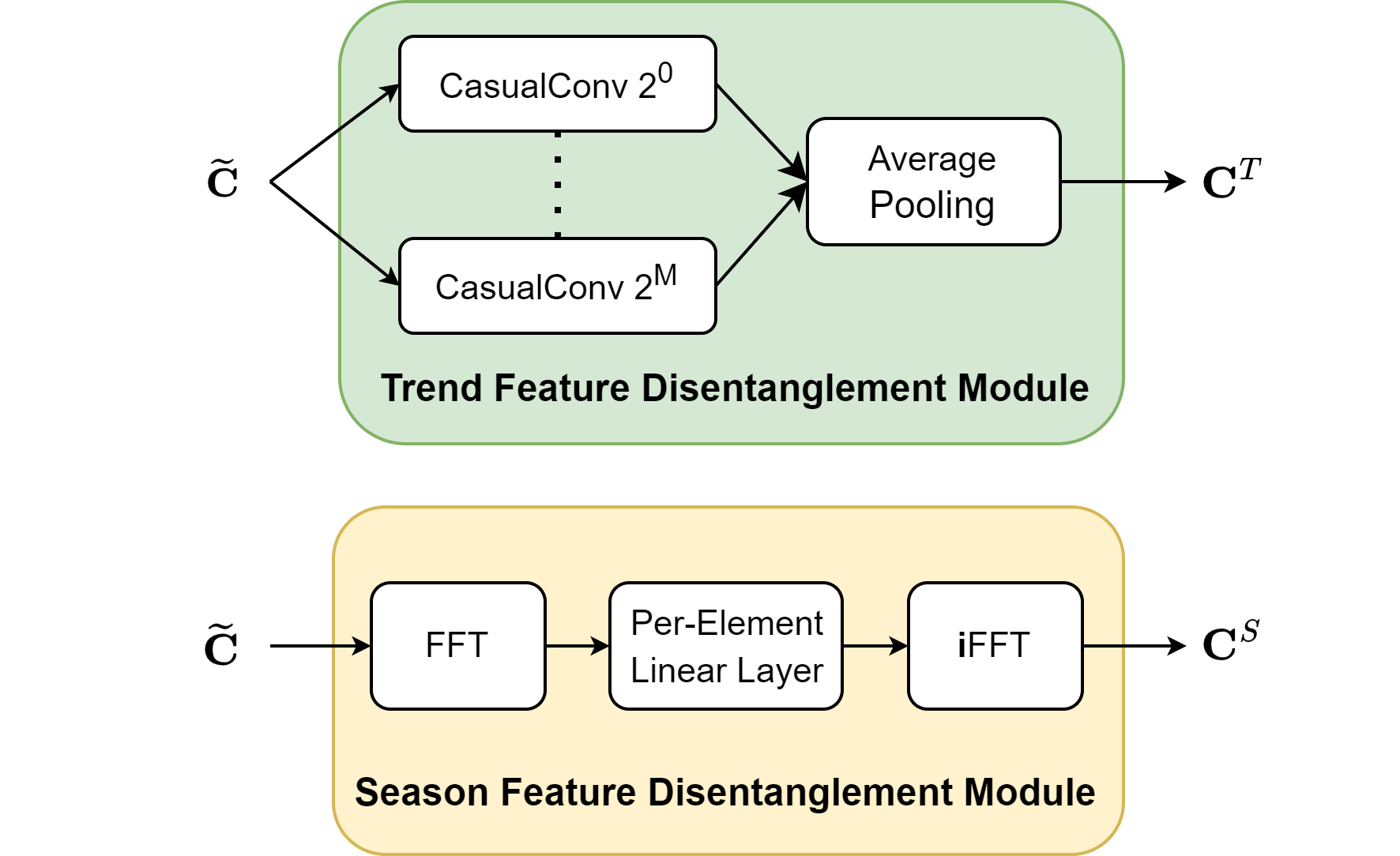
Figure 2: The architecture of our proposed Trend-Season Feature Disentanglement Module. The upper box details the TFD Module implemented by a stack of casual convolution layers with different kernel sizes. The lower one details the SFD Module implemented by FFT and iFFT layers.

The Trend-Season Disentanglement Module, depicted in Fig. 2, plays an important role in computing conditional information when the diffusion model is applied for spatiotemporal imputation. Drawing inspiration from previous research by [24], we conceptualize time series as a combination of trend, season, and error variables, employing this structure as a foundation to learn explainable temporal dependencies. Our objective is to derive disentangled representations for the trend and seasonal components, represented as $\mathbf{C}^{Tem}=[\mathbf{C}^{T};\mathbf{C}^{S}]\in\mathbb{R}^{L\times(d\cdot N)}$, where $\mathbf{C}^{T}\in\mathbb{R}^{L\times(d_{T}\cdot N)}$ and $\mathbf{C}^{S}\in\mathbb{R}^{L\times(d_{S}\cdot N)}$, and $d=d_{T}+d_{S}$. The Trend Feature Disentanglement (TFD) Module is designed as a mixture of $M+1$ autoregressive experts, with $M=\lfloor log_{2}(L/2)\rfloor$. Each expert is realized through a 1-dimensional causal convolution, with $d$ input channels and $d_{T}$ output channels. The kernel size for the $m$-th expert is set to $2^{m}$. Every expert generates an output matrix $\widetilde{\mathbf{C}}^{T,m}=CasualConv(\widetilde{\mathbf{C}},2^{m})$. To synthesize the final trend representations, we apply an average-pooling operation over the collective outputs of these experts.

$$\mathbf{C}^{T}=AvgPool(\widetilde{\mathbf{C}}^{T,0},\widetilde{\mathbf{C}}^{T,1},\cdots,\widetilde{\mathbf{C}}^{T,M})=\frac{1}{M+1}\sum^{M}_{m=0}\widetilde{\mathbf{C}}^{T,i}$$ (5)

Building on the approach established by [25], we have developed a Season Feature Disentanglement (SFD) Module incorporating a learnable Fourier layer for extracting seasonal features from the frequency domain. This module includes a discrete Fourier transform (DFT), which converts time domain representations into their frequency domain counterparts, denoted as $\mathcal{F}(\widetilde{\mathbf{C}})\in\mathbb{C}^{F\times(d\cdot N)}$. Here, $F=\lfloor L/2\rfloor+1$ represents the number of frequencies captured. The subsequent learnable Fourier layer facilitates interactions within the frequency domain. This layer executes a per-element linear transformation across frequencies, utilizing a distinct set of complex-valued parameters for each frequency. Following the frequency domain processing, we revert the representations to the time domain via an inverse DFT. The resultant output matrix, $\mathbf{C}^{S}\in\mathbb{R}^{L\times(d_{S}\cdot N)}$, embodies the seasonal representation. The $i$, $k$-th element of this output can be represented as follows:

$$\mathbf{C}_{i,k}^{S}=\mathcal{F}^{-1}\left(\sum^{d}_{j=1}\mathbf{A}_{i,j,k}\mathcal{F}(\widetilde{\mathbf{C}}_{i,j}+\mathbf{B}_{i,k})\right)$$ (6)

where $\mathbf{A}\in\mathbb{C}^{F\times(d\cdot N)\times(d_{S}\cdot N)}$ and $\mathbf{B}\in\mathbb{C}^{F\times(d_{S}\cdot N)}$ represent the parameters of the per-element linear layer.

Once the disentangled temporal representation $\mathbf{C}^{Tem}$ is obtained, we employ a Spatial Feature Extraction Module to learn the spatial dependencies. This module is tasked with generating the final conditional feature, denoted as $\mathbf{C}^{Con}\in\mathbb{R}^{N\times L\times d}$. The formalization of this process is as follows:

$$\begin{split}\mathbf{C}^{Spa}&=\mathcal{G}(\mathbf{C}^{Tem},A)\\ \mathbf{C}^{Con}&=MLP(Norm(\mathbf{C}^{Spa}+\mathbf{C}^{Tem})\end{split}$$ (7)

In our formulation, $\mathcal{G}(\cdot)$ denotes the GNN encoder, a component that can be implemented using any graph neural network architecture. In line with prior research [23], we have chosen to integrate the graph convolution module from Graph Wavenet [5]. This module utilizes an adjacency matrix encompassing a bidirectional distance-based matrix and an adaptive learnable matrix, facilitating effective spatial information processing within our model.

III-C2 Noise Estimation Module

Our noise estimation module is crucial when employing the diffusion model, particularly by leveraging conditional information. Gaussian noise in the noisy samples can significantly distort their alignment with the spatiotemporal distribution, posing challenges in directly learning spatiotemporal dependencies from a mixture of conditional and noisy data. To address this, our noise estimation module harnesses an attention mechanism to discern global spatiotemporal correlations. This mechanism effectively mitigates the complexities associated with learning spatiotemporal dependencies that are otherwise exacerbated by the randomness of the sample noise.

This module processes several inputs, including the noisy information $\mathbf{H}^{in}=Conv(\mathbf{C}||\widetilde{\mathbf{X}^{t}})$, the conditional feature $\mathbf{C}^{Con}$, and the adjacency matrix $A$. To thoroughly capture the spatiotemporal correlations in the missing data, we first derive temporal features $\mathbf{H}^{Tem}$ via a temporal dependency learning module denoted as $\gamma_{T}(\cdot)$. Subsequently, these temporal features are integrated using a spatial dependency learning module, $\gamma_{S}(\cdot)$. The formulation of this process is as follows:

$$\begin{split}\mathbf{H}^{tem}=&\gamma_{T}(\mathbf{H}^{in})=Attn_{tem}(\mathbf{H}^{in})\\ \mathbf{H}^{spa}=&\gamma_{S}(\mathbf{H}^{tem},A)\\ =&MLP(Norm(Attn_{spa}(\mathbf{H}^{tem})+\mathbf{H}^{tem})\\ &+Norm(\mathcal{G}(\mathbf{H}^{tem},A)+\mathbf{H}^{tem}))\end{split}$$ (8)

where $Attn_{tem}(\cdot)$ signifies the global temporal attention mechanism. To implement $Attn(\cdot)$, we employ the dot-product multi-head self-attention mechanism designed in the Transformer architecture. $\mathbf{H}^{tem}$ and $\mathbf{H}^{spa}$ belongs to $\mathbb{R}^{N\times L\times d}$, represent the outputs from the temporal and spatial dependency learning modules, respectively.

In Eq. (8), the learning of spatiotemporal dependencies is conducted on the combination of conditional noisy information $\mathbf{H}^{in}$. As the diffusion step $t$ nears $T$, increasing noise in the sample $\widetilde{\mathbf{X}^{t}}$ challenges learning spatiotemporal dependencies. To mitigate the influence of $\widetilde{\mathbf{X}^{t}}$ and to facilitate its transformation into Gaussian noise, we modify the input for the attention mechanisms $Attn_{tem}(\cdot)$ and $Attn_{spa}(\cdot)$. These components are responsible for computing attention weights, now utilizing the conditional feature $\mathbf{C}^{Con}$. Specifically, taking $Attn_{tem}(\cdot)$ as an example, we formulate it as follows:

$$\begin{split}Attn_{tem}(\mathcal{A}_{\mathcal{T}},\mathcal{V}_{\mathcal{T}})&=SoftMax\left(\frac{\mathcal{Q}_{\mathcal{T}}\mathcal{K}_{\mathcal{T}}^{T}}{\sqrt{d}}\right)\cdot\mathcal{V}_{\mathcal{T}}\\ \mathcal{Q}_{\mathcal{T}}&=\mathbf{C}^{Con}\cdot W_{\mathcal{T}}^{Q}\\ \mathcal{K}_{\mathcal{T}}&=\mathbf{C}^{Con}\cdot W_{\mathcal{T}}^{K}\\ \mathcal{V}_{\mathcal{T}}&=\mathbf{H}^{in}\cdot W_{\mathcal{T}}^{V}\\ \end{split}$$ (9)

where $W_{\mathcal{T}}^{Q},W_{\mathcal{T}}^{K},W_{\mathcal{T}}^{V}\in\mathbb{R}^{d\times d}$ are learnable projection parameters. The $Attn_{spa}(\mathcal{A}_{\mathcal{S}},\mathcal{V}_{\mathcal{S}})$ calculates the attention weight in the same way with the $Attn_{tem}$.

The noise estimation module consists of multiple stacked layers. The outputs $\mathbf{H}^{spa}$ from each layer are entered into residual and skip connections subsequent to a gated activation unit. The residual connection is applied as the input for the subsequent layer, while the skip connections from each layer are aggregated. This aggregated output is then processed through two layers of 1-d convolution to derive the output of the noise prediction model, $\epsilon_{\theta}$. Importantly, this output exclusively retains the values pertinent to the imputation target.

III-C3 Contrastive Learning Strategy

In our endeavor to enhance the robustness and stability of the diffusion model, we have developed contrastive learning strategy to address challenges in the generation process. This strategy involves the creation of two distinct residual layer modules, each designed to produce different generative outputs while utilizing the same conditional features as references. These outputs are positive samples relative to each other, and an output randomly sampled from the same batch is treated as a negative sample. The incorporation of this contrastive learning approach necessitates a modification to the loss function, which is articulated in the subsequent equation:

$$\begin{split}\mathcal{L}_{cl}&=-\frac{1}{N}\sum_{i=1}^{N}\log\frac{\exp\left(\frac{\text{sim}(x_{i},y_{i}^{+})}{\tau}\right)}{\sum_{j=1}^{2N}\exp\left(\frac{\text{sim}(x_{i},y_{j}^{-})}{\tau}\right)}\\ \mathcal{L}_{rl}&=\mathcal{L}(\theta)\\ \mathcal{L}&=\mathcal{L}_{rl}+\alpha\mathcal{L}_{cl}\end{split}$$ (10)

In Eq. (10), we incorporate the widely used Noise Contrastive Estimation (NCE) Loss from the domain of unsupervised learning to compute the contrastive loss, denoted as $\mathcal{L}_{cl}$. Here, $N$ represents the number of samples in a batch, $\text{sim}(\cdot)$ indicates the cosine similarity function, and $\tau$ is the temperature coefficient. The terms $x_{i}$, $y_{i}^{+}$, and $y_{j}$ correspond to the target, positive, and negative samples. Additionally, the reconstruction loss, $\mathcal{L}_{rl}$, is computed in accordance with Eq. (4). The overall model loss, $\mathcal{L}$, is formulated as a weighted amalgamation of the contrastive and reconstruction losses, with the weight $\alpha$ dictating the relative importance of the contrastive loss component.

IV Experiments

In this section, we report our evaluation of our model C²TSD, including the experimental settings (datasets, baselines, evaluation metrics) and results analysis.

IV-A Datasets

In evaluating C²TSD, we introduce three distinct datasets, each pertinent to the spatiotemporal imputation field, as highlighted in prior research [15]. The datasets include:

• AQI-36 [44]: includes hourly PM2.5 measurements recorded by 36 monitoring stations located in Beijing. The data spans a period of 12 months.

• PEMS-BAY [45]: includes traffic speed data collected from 325 sensors located on highways in the San Francisco Bay Area. The duration of data collection is 6 months.

• METR-LA [45]: includes traffic speed data gathered by 207 sensors located on highways in Los Angeles County. The duration of data collection is 4 months.

Each dataset in our study exhibits distinct characteristics and poses specific challenges relevant to spatiotemporal imputation. This diversity renders them suitable for evaluating the efficacy and adaptability of the C²TSD framework.

IV-B Baselines

To rigorously evaluate the effectiveness of our C²TSD model, we undertook a comprehensive comparative analysis with a selection of established and state-of-the-art models in the domain of spatiotemporal imputation. The baseline models encompass a wide array of methodologies, ranging from statistical approaches (such as MEAN, DA, kNN, Linear) and machine learning techniques (including MICE, VAR, KF) to matrix factorization methods (TRMF, BATF), advanced deep learning models (BRITS, GRIN, rGAIN), and generative strategies (V-RIN, GP-VAE, CSDI, PriSTI). A succinct overview of each baseline model is provided below:

• MEAN: This method imputes missing values using each node’s historical average value.

• DA: Daily averages at relevant time steps for imputation.

• kNN: This approach calculates and uses the average value of geographically proximate nodes for imputation.

• Linear: Linear interpolation of the time series for each node, as implemented by torchcde.

• KF: A Kalman Filter is employed to impute time series data for each node, as implemented by.

• MICE [46]: Multivariate Imputation by Chained Equations, based on Fully Conditional Specification, where a separate model imputes each incomplete variable.

• VAR: A vector autoregressive model used as a single-step predictor.

• TRMF [27]: Temporal Regularized Matrix Factorization.

• BATF [28]: Bayesian Augmented Tensor Factorization integrates spatiotemporal domain knowledge.

• BRITS [14]: A bidirectional RNN-based method for multivariate time series imputation.

• GRIN [15]: This model uses a bidirectional GRU combined with a graph convolution network for multivariate time series imputation.

• rGAIN [30]: An approach that extends the GAIN model with a bidirectional recurrent encoder-decoder structure.

• V-RIN [47]: A method to improve deterministic imputation using VAE. The quantified uncertainty provides the probability imputation result.

• GP-VAE [48]: A probabilistic imputation method for time series that combines a Variational Autoencoder with Gaussian processes.

• CSDI [22]: A probability imputation method based on a conditional diffusion probability model, which treats different nodes as multiple feature dependencies.

• PriSTI [23]: A conditional diffusion framework with a feature extraction module to calculate the spatiotemporal attention weights.

Each baseline model in our study exhibits a different type of model for spatiotemporal imputation. These diverse models provide a comprehensive scope for evaluating our C²TSD model, enabling a comprehensive assessment of its performance relative to various approaches in the field.

IV-C Evaluation Metrics

In line with the methodology outlined in previous research [23], we utilize three well-established evaluation metrics to gauge the performance of our proposed C²TSD model in the context of spatiotemporal imputation.

Among these, the primary metrics are calculating the Mean Absolute Error (MAE) and Mean Squared Error (MSE) across the imputation window. Both MAE and MSE provide a quantitative measure of the absolute error between the values imputed by our model and the actual ground truth. These metrics are crucial for evaluating the accuracy and reliability of our model in accurately predicting missing values in spatiotemporal data.

Additionally, we utilize the Continuous Ranked Probability Score (CRPS) [49] to assess the similarity between the estimated probability distribution and its observed values. For a given missing value $x$ with its estimated probability distribution $D$, the CRPS quantifies the compatibility of $x$ with $D$. This compatibility is determined through the integral of the quantile loss $\Lambda_{\alpha}$, which is defined as:

$$\begin{split}\text{CRPS}(D^{-1},x)&=\int^{1}_{0}2\Lambda_{\alpha}(D^{-1}(\alpha),x)d\alpha\\ \Lambda_{\alpha}(D^{-1}(\alpha),x)&=(\alpha-\mathbb{1}_{x<D^{-1}(\alpha)})(x-D^{-1}(\alpha))\end{split},$$ (11)

where the parameter $\alpha\in[0,1]$ represents the quantile levels, while $D^{-1}(\alpha)$ denotes the $\alpha$-quantile of the distribution $D$, and $\mathbb{1}$ serves as the indicator function. Consistent with the approach outlined in prior research [23], we generate 100 samples to simulate the distribution of missing values in our model accurately. The quantile losses are calculated for discretized quantile levels using intervals of 0.05. This calculation process is formalized as follows:

$$\text{CRPS}(D^{-1},x)\simeq\sum^{19}_{i=1}2\Lambda_{i\times 0.05}(D^{-1}(i\times 0.05),x)/19.$$ (12)

We calculate the Continuous Ranked Probability Score (CRPS) for each estimated missing value to evaluate our model’s probabilistic forecasting accuracy. The average CRPS across all such values is then used as the primary metric for assessment, which is formalized as:

$$\text{CRPS}(D,\widetilde{X})=\frac{\sum_{{x}\in\widetilde{X}}\text{CRPS}(D^{-1},{x})}{|\widetilde{X}|}.$$ (13)

IV-D Experiment Design

IV-D1 Datasets Split

In alignment with the dataset division methodology employed by [15], we partitioned the data into training, validation, and test sets for our evaluation. For the AQI-36 dataset, March, June, September, and December were selected as the test dataset. The validation set encompasses the last 10% of the data from February, May, August, and November, while the remaining data forms the training set. As for the PEMS-BAY and METR-LA datasets, a chronological division strategy was applied. Here, 70% of the data was allocated to the training set, 10% to the validation set, and the final 20% designated as the test dataset. The data split method shows how our model works across various temporal situations within each dataset. Such an approach is critical for assessing the robustness and generalizability of the model in real-world scenarios.

IV-D2 Imputation Strategies

For the AQI-36 dataset, we aligned our evaluation approach with the strategy established in previous work by [50]. This strategy mimics the distribution of real missing data, providing a realistic and relevant context for assessing imputation performance. We implemented a distinct evaluation methodology for the traffic datasets PEMS-BAY and METR-LA. This involved the creation of a mask matrix, as suggested by [15], to manually inject missing values for evaluation purposes. We employed two distinct missing patterns in this process: (1) Point missing, where we randomly masked 25% of the observations, and (2) Block missing, which entailed randomly masking 5% of the observations and then further masking consecutive observations ranging from 1 to 4 hours for each sensor with a probability of 0.15%. All three datasets inherently contain missing data besides these artificially induced missing values. The AQI-36 dataset has an inherent missing data rate of 13.24%, while PEMS-BAY and METR-LA have rates of 0.02% and 8.10%, respectively. However, our evaluations are specifically focused on the missing data segments that we artificially introduced into the test portions of each dataset. This approach allows for a controlled and precise assessment of our model’s imputation capabilities, ensuring that the evaluation is directly attributable to the model’s performance rather than external factors or pre-existing data gaps.

IV-D3 Hyperparameters

The training process for our model was executed on a single Nvidia A40 GPU, equipped with 48 GB of memory, ensuring efficient computation and handling of the complex model architecture. To optimize the parameters of C²TSD, we applied the Adam optimizer, a widely recognized and effective optimization algorithm known for its adaptability and robust performance in various deep learning-based model training. Additionally, we incorporated a cosine annealing learning rate decay strategy. This strategy involves gradually reducing the learning rate, following a cosine function, to fine-tune the model’s performance over time. The learning rate is set to $10^{-3}$ and decays to $10^{-5}$, balancing effective learning and preventing overshooting during optimization. The parameter $T_{max}$ in this context denotes the maximum number of epochs, which is a critical factor in determining the duration and progression of the learning rate decay. The diffusion step $T$ is set to 100 for the AQI-36 dataset and 50 for two traffic datasets. The minimum noise level $\beta_{1}$ is $10^{-4}$ and maximum noise level $\beta_{T}$ is $0.2$. This configuration of hyperparameters and training setup was carefully selected to optimize the learning process of C²TSD, ensuring that the model efficiently learns from the data while maintaining a high degree of accuracy and generalizability in its predictions.

IV-E Results

TABLE I: The results of MAE and MSE metrics for spatiotemporal imputation in three datasets with different missing patterns. The best result is boldfaced. The second-best result is underlined. The Improv. denotes the improvement of our proposed C²TSD compared with the performance of the best baseline. - denotes the improvement is equal to or smaller than 0.

Method	AQI-36		PEMS-BAY				METR-LA
			Point missing		Block missing		Point missing		Block missing
	MAE	MSE	MAE	MSE	MAE	MSE	MAE	MSE	MAE	MSE
Mean	53.48	4578.08	5.42	86.59	5.46	87.56	7.56	142.22	7.48	139.54
DA	50.51	4416.10	3.35	44.50	3.30	43.76	14.57	448.66	14.53	445.08
kNN	30.21	2892.31	4.30	49.80	4.30	49.90	7.88	129.29	7.79	124.61
Linear	14.46	673.92	0.76	1.74	1.54	14.14	2.43	14.75	3.26	33.76
KF	54.09	4942.26	5.68	93.32	5.64	93.19	16.66	529.96	16.75	534.69
MICE	30.37	2594.06	3.09	31.43	2.94	28.28	4.42	55.07	4.22	51.07
VAR	15.64	833.46	1.30	6.52	2.09	16.06	2.69	21.10	3.11	28.00
TRMF	15.46	1379.05	1.85	10.03	1.95	11.21	2.86	20.39	2.96	22.65
BATF	15.21	662.87	2.05	14.90	2.05	14.48	3.58	36.05	3.56	35.39
BRITS	14.50	622.36	1.47	7.94	1.70	10.50	2.34	16.46	2.34	17.00
GRIN	12.08	523.14	0.67	1.55	1.14	6.60	1.91	10.41	2.03	13.26
V-RIN	10.00	838.05	1.21	6.08	2.49	36.12	3.96	49.98	6.84	150.08
GP-VAE	25.71	2589.53	3.41	38.95	2.86	26.80	6.57	127.26	6.55	122.33
rGAIN	15.37	641.92	1.88	10.37	2.18	13.96	2.83	20.03	2.90	21.67
CSDI	9.51	352.46	0.57	1.12	0.86	4.39	1.79	8.96	1.98	12.62
PriSTI	9.22	324.95	0.57	1.09	0.78	3.50	1.76	8.63	1.89	11.21
C2TSD	9.09	309.81	0.57	1.09	0.81	3.23	1.70	8.47	1.79	10.65
Improv.	1.43%	4.89%	-	-	-	8.48%	3.28%	1.95%	5.91%	5.24%

TABLE II: The CRPS result for spatiotemporal imputation. Point and Block denote missing patterns, same with Table I

Method	AQI-36	PEMS-BAY		METR-LA
		Point	Block	Point	Block
V-RIN	0.3154	0.0191	0.3940	0.0781	0.1283
GP-VAE	0.3377	0.0568	0.0436	0.0977	0.1118
CSDI	0.1056	0.0067	0.0127	0.0235	0.0260
PriSTI	0.1025	0.0067	0.0094	0.0231	0.0249
C2TSD	0.0995	0.0067	0.0097	0.0223	0.0237

IV-E1 Overall Performance

In our study, we first evaluated the spatiotemporal imputation performance of our proposed method, C²TSD, compared with various baseline models. To accommodate the varied capabilities of these methods, particularly in terms of probabilistic outputs, we employed different metrics for a comprehensive assessment. For methods incapable of providing the probability distribution of missing values, we presented deterministic imputation results quantified using MAE and MSE. These results are detailed in Table I. This approach ensures a fair and direct comparison of the imputation accuracy among different models. In addition, for models that can simulate the probability distribution of missing values, including V-RIN, GP-VAE, CSDI, PriSTI, and our C²TSD, we showcased the CRPS results in Table II. This metric is particularly insightful for evaluating the quality of probabilistic forecasts. To simulate the probability distribution, we generated 100 samples for each missing value, and the deterministic imputation result was determined by taking the median of these samples. By employing this dual metric evaluation approach, we aimed to capture both the imputation methods’ deterministic accuracy and probabilistic quality. This analysis allows us to draw a more nuanced understanding of each method’s relative strengths and weaknesses, including our own C²TSD, in spatiotemporal imputation.

The results from Table I and Table II demonstrate the superior performance of our proposed method, C²TSD, across various missing data scenarios and datasets, outperforming other baseline models. Our method shows better performance compared to the high-performing baseline, PriSTI. Analysis of the results in Table I reveals that traditional statistical and machine learning-based methods underperform across all datasets. Such methods typically depend on strict assumptions, like stability or seasonality in time series, to predict missing values. However, these assumptions fail to capture real-world scenarios’ complex temporal and spatial dependencies. Additionally, matrix factorization-based methods exhibit less satisfactory performance, likely due to their reliance on the low-rank assumption. In deep learning-based methods, GRIN outperforms RNN-based methods (such as rGAIN and BRITS) by utilizing spatial dependencies. Despite this, GRIN’s performance still lags behind diffusion-based methods like CSDI and PriSTI, possibly due to the inherent limitations of error accumulation in recurrent structure models. Regarding deep generative models, it is evident that VAE-based methods (V-RIN and GP-VAE) are not as effective as diffusion-based methods (CSDI, PriSTI, and our C²TSD). Our method, C²TSD, surpasses PriSTI in most metrics across various missing patterns and datasets, with only two metrics where it ranks second. This achievement validates our approach of employing conditional features to disentangle trend and seasonal elements and using a contrastive learning strategy, which collectively enhances the imputation performance of diffusion-based methods. The results highlight the positive impact of our proposed innovations on improving spatiotemporal imputation.

Our analysis includes the Continuous Ranked Probability Score (CRPS) metric results for four generative baselines and our method, C²TSD, shown in Table II. The CRPS results indicate that diffusion-based methods exhibit superior performance in terms of CRPS scores when compared to VAE-based approaches. The CRPS helps understand how accurately a model captures the uncertainty in predictions. This metric extends beyond the mere accuracy of predictions, delving into the reliability and robustness of the forecasts. CRPS assesses not just the central tendency of the predictions, such as the mean or median, but also considers the shape and spread of the prediction distribution. Unlike deterministic metrics focusing solely on prediction accuracy, CRPS provides a more holistic evaluation by examining the alignment of the generated simulated distribution with the actual distribution of the time series data. Our proposed method, C²TSD, demonstrates proficiency in accurate prediction and generates distributions that closely mirror the true distribution of real-time series data. The ability of C²TSD to achieve solid accuracy and represent prediction uncertainty well demonstrates its effectiveness as a generative model for spatiotemporal imputation.

IV-E2 Ablation Study

TABLE III: Ablation Studies reported the MAE metric on AQI-36 and METR-LA datasets. Point and Block denote missing patterns, same with Table I

Method	AQI-36	METR-LA
		Point	Block
C2TSD	9.09	1.74	1.88
w/o CL	10.18	2.18	2.27
w/o TFD	10.06	2.07	2.14
w/o SFD	9.80	2.09	2.07

We conducted ablation studies by comparing our method with the following variants:

• w/o CL: Remove the contrastive loss $\mathcal{L}_{cl}$ in Eq. (10), only calculate the gradient of the reconstruction loss $\mathcal{L}_{rl}$;

• w/o TFD: Remove the trend representation $\mathbf{C}^{T}$ in Eq. (5) in the conditional information construction module, only keep the season representation $\mathbf{C}^{S}$ for using to construct the conditional information;

• w/o SFD: Similar to the previous variant, remove the season representation $\mathbf{C}^{S}$ in Eq. (6) in the conditional information construction module, only keep the trend representation $\mathbf{C}^{T}$ for the conditional information.

Given the similarities in spatiotemporal dependencies and missing patterns of the two traffic datasets, AQI-36 and METR-LA, we conducted an ablation study to assess the impact of various components within our proposed framework, C²TSD. The Mean Absolute Error (MAE) results of the ablation study are presented in Table III. Analyzing the results from both datasets across different missing patterns, it is evident that the individual modules in C²TSD significantly contribute to the overall imputation performance. The ablation studies yield consistent conclusions across different datasets. Among the various components of C²TSD, the contrastive learning strategy emerges as the most influential, with the most considerable drop in performance observed upon its removal. Additionally, when comparing the results of removing the trend representation (w/o Trend) versus the seasonal representation (w/o Season), we observe a more pronounced performance degradation in the absence of the trend component, particularly for the AQI-36 dataset and the block missing pattern in the METR-LA dataset. This observation suggests that the seasonal representation contributes less to the imputation accuracy in the context of the AQI-36 dataset, where complex factors influence PM2.5 concentration and lack clear periodicity. Conversely, the trend feature is more readily discernible for the METR-LA dataset, especially under point missing patterns, as average traffic speed typically does not exhibit rapid fluctuations over short intervals. This differential impact highlights the importance of features in spatiotemporal data imputation.

IV-E3 Hyperparameter Analysis

Figure 3: The sensitivity study of three key parameters for three datasets.

In our research, we conducted experiments on crucial hyperparameters within the C²TSD framework, aiming to uncover their optimal configurations and assess the model’s response to parameter adjustments. We focused on three essential hyperparameters: the maximum noise level $\beta_{T}$, the dimensionality of the hidden state’s channel size $d$, and the weight of the contrastive loss $\alpha$. The outcomes of this comprehensive study are showcased in Fig. 3. The parameter $\beta_{T}$ regulates the noise intensity introduced during the diffusion steps. A significantly low $\beta_{T}$ might result in a tediously slow diffusion process, necessitating more iterations for the model to effectively transition data towards the desired distribution. On the other hand, an elevated $\beta_{T}$ could lead to an overly rapid diffusion, potentially erasing crucial information and complicating the model’s inversion process. Our analysis, as shown in Fig. 3, reveals that for the AQI-36 and PEMS-BAY datasets, the model sustains satisfactory performance at a $\beta_{T}$ of 0.2 or above. For the METR-LA dataset, the model’s MAE metric exhibits stability with $\beta_{T}$ values ranging from 0.1 to 0.4. Consequently, we selected a $\beta_{T}$ of 0.2 for our principal experiments to ensure optimal outcomes. Regarding the channel size $d$, it plays a pivotal role in defining the model’s capacity to encode information. Fig. 3 demonstrates that the model records the lowest MAE with a channel size of 16 for the AQI-36 dataset and 64 for the PEMS-BAY and METR-LA datasets. A channel size too small may not provide sufficient capacity for learning, while a size too large could incorporate unnecessary noise into the embeddings, detracting from the model’s ability to capture spatiotemporal dependencies efficiently. Given that the AQI-36 dataset has a smaller number of features than the traffic datasets, a smaller channel size is necessary to learn spatiotemporal embeddings effectively. Lastly, the contrastive loss weight $\alpha$ balances the reconstruction loss and contrastive loss. An excessively high $\alpha$ may lead the model to disregard the reconstruction loss, adversely affecting performance. According to Fig. 3, optimal performance for the model is attained with an $\alpha$ of 0.1 for the AQI-36 and METR-LA datasets and 0.2 for the PEMS-BAY dataset. Thus, based on our sensitivity analysis, we have set the three key hyperparameters to their ideal values to maximize the model’s efficiency.

V Conclusion

We introduce C²TSD, an effective conditional diffusion framework that integrates contrastive learning and trend-season disentanglement for spatiotemporal imputation. This model predicts missing values by employing a diffusion process enhanced by contrastive learning and utilizes disentangled trend and seasonal dependencies as key conditional features to guide this process. Our model has shown enhanced performance compared to state-of-the-art baselines across various missing data patterns. Looking ahead, exploring additional conditional features could further refine the guidance of the diffusion process. By investigating alternative conditional features, we aim to improve the robustness and reliability of diffusion models, thereby advancing the field of generative models and their applications in spatiotemporal imputation.

References

- [1] Q. Li, J. Tan, J. Wang, and H. Chen, “A multimodal event-driven lstm model for stock prediction using online news,” IEEE Transactions on Knowledge and Data Engineering, vol. 33, no. 10, pp. 3323–3337, 2020.
- [2] D. A. Tedjopurnomo, Z. Bao, B. Zheng, F. M. Choudhury, and A. K. Qin, “A survey on modern deep neural network for traffic prediction: Trends, methods and challenges,” IEEE Transactions on Knowledge and Data Engineering, vol. 34, no. 4, pp. 1544–1561, 2020.
- [3] F. Di Martino and F. Delmastro, “Explainable ai for clinical and remote health applications: a survey on tabular and time series data,” Artificial Intelligence Review, vol. 56, no. 6, pp. 5261–5315, 2023.
- [4] P. Bauer, A. Thorpe, and G. Brunet, “The quiet revolution of numerical weather prediction,” Nature, vol. 525, no. 7567, pp. 47–55, 2015.
- [5] Z. Wu, S. Pan, G. Long, J. Jiang, and C. Zhang, “Graph wavenet for deep spatial-temporal graph modeling,” in Proceedings of the 28th International Joint Conference on Artificial Intelligence, ser. IJCAI’19. AAAI Press, 2019, p. 1907–1913.
- [6] Z. Han, J. Zhao, H. Leung, K. F. Ma, and W. Wang, “A review of deep learning models for time series prediction,” IEEE Sensors Journal, vol. 21, no. 6, pp. 7833–7848, 2019.
- [7] H. Ismail Fawaz, G. Forestier, J. Weber, L. Idoumghar, and P.-A. Muller, “Deep learning for time series classification: a review,” Data mining and knowledge discovery, vol. 33, no. 4, pp. 917–963, 2019.
- [8] A. Blázquez-García, A. Conde, U. Mori, and J. A. Lozano, “A review on outlier/anomaly detection in time series data,” ACM Computing Surveys (CSUR), vol. 54, no. 3, pp. 1–33, 2021.
- [9] Z. Che, S. Purushotham, K. Cho, D. Sontag, and Y. Liu, “Recurrent neural networks for multivariate time series with missing values,” Scientific reports, vol. 8, no. 1, pp. 1–12, 2018.
- [10] C. F. Ansley and R. Kohn, “On the estimation of arima models with missing values,” in Time Series Analysis of Irregularly Observed Data: Proceedings of a Symposium held at Texas A & M University, College Station, Texas February 10–13, 1983. Springer, 1984, pp. 9–37.
- [11] R. H. Shumway and D. S. Stoffer, “An approach to time series smoothing and forecasting using the em algorithm,” Journal of time series analysis, vol. 3, no. 4, pp. 253–264, 1982.
- [12] T. Hastie, R. Tibshirani, J. H. Friedman, and J. H. Friedman, The elements of statistical learning: data mining, inference, and prediction. Springer, 2009, vol. 2.
- [13] J. Wang, W. Du, W. Cao, K. Zhang, W. Wang, Y. Liang, and Q. Wen, “Deep learning for multivariate time series imputation: A survey,” arXiv preprint arXiv:2402.04059, 2024.
- [14] W. Cao, D. Wang, J. Li, H. Zhou, L. Li, and Y. Li, “Brits: Bidirectional recurrent imputation for time series,” Advances in neural information processing systems, vol. 31, 2018.
- [15] A. Cini, I. Marisca, and C. Alippi, “Filling the g_ap_s: Multivariate time series imputation by graph neural networks,” in International Conference on Learning Representations, 2022.
- [16] Y. Liu, R. Yu, S. Zheng, E. Zhan, and Y. Yue, “Naomi: Non-autoregressive multiresolution sequence imputation,” Advances in neural information processing systems, vol. 32, 2019.
- [17] Y. Wu, J. Wang, X. Miao, W. Wang, and J. Yin, “Differentiable and scalable generative adversarial models for data imputation,” IEEE Transactions on Knowledge and Data Engineering, 2023.
- [18] X. Miao, Y. Wu, J. Wang, Y. Gao, X. Mao, and J. Yin, “Generative semi-supervised learning for multivariate time series imputation,” in Proceedings of the AAAI conference on artificial intelligence, vol. 35, no. 10, 2021, pp. 8983–8991.
- [19] L. Lin, Z. Li, R. Li, X. Li, and J. Gao, “Diffusion models for time-series applications: a survey,” Frontiers of Information Technology & Electronic Engineering, pp. 1–23, 2023.
- [20] J. Ho, A. Jain, and P. Abbeel, “Denoising diffusion probabilistic models,” Advances in neural information processing systems, vol. 33, pp. 6840–6851, 2020.
- [21] Y. Song, J. Sohl-Dickstein, D. P. Kingma, A. Kumar, S. Ermon, and B. Poole, “Score-based generative modeling through stochastic differential equations,” in International Conference on Learning Representations, 2021.
- [22] Y. Tashiro, J. Song, Y. Song, and S. Ermon, “Csdi: Conditional score-based diffusion models for probabilistic time series imputation,” Advances in Neural Information Processing Systems, vol. 34, pp. 24 804–24 816, 2021.
- [23] M. Liu, H. Huang, H. Feng, L. Sun, B. Du, and Y. Fu, “Pristi: A conditional diffusion framework for spatiotemporal imputation,” in 2023 IEEE 39th International Conference on Data Engineering (ICDE). Los Alamitos, CA, USA: IEEE Computer Society, 2023, pp. 1927–1939.
- [24] J. Qiu, S. R. Jammalamadaka, and N. Ning, “Multivariate bayesian structural time series model.” J. Mach. Learn. Res., vol. 19, no. 1, pp. 2744–2776, 2018.
- [25] G. Woo, C. Liu, D. Sahoo, A. Kumar, and S. Hoi, “Cost: Contrastive learning of disentangled seasonal-trend representations for time series forecasting,” in International Conference on Learning Representations, 2022.
- [26] A. Blázquez-García, K. Wickstrøm, S. Yu, K. Ø. Mikalsen, A. Boubekki, A. Conde, U. Mori, R. Jenssen, and J. A. Lozano, “Selective imputation for multivariate time series datasets with missing values,” IEEE Transactions on Knowledge and Data Engineering, 2023.
- [27] H.-F. Yu, N. Rao, and I. S. Dhillon, “Temporal regularized matrix factorization for high-dimensional time series prediction,” Advances in neural information processing systems, vol. 29, 2016.
- [28] X. Chen, Z. He, Y. Chen, Y. Lu, and J. Wang, “Missing traffic data imputation and pattern discovery with a bayesian augmented tensor factorization model,” Transportation Research Part C: Emerging Technologies, vol. 104, pp. 66–77, 2019.
- [29] S. Liu, X. Li, G. Cong, Y. Chen, and Y. Jiang, “Multivariate time-series imputation with disentangled temporal representations,” in International Conference on Learning Representations, 2022.
- [30] J. Yoon, J. Jordon, and M. Schaar, “Gain: Missing data imputation using generative adversarial nets,” in International conference on machine learning. PMLR, 2018, pp. 5689–5698.
- [31] Y. Luo, X. Cai, Y. Zhang, J. Xu et al., “Multivariate time series imputation with generative adversarial networks,” Advances in neural information processing systems, vol. 31, 2018.
- [32] Y. Luo, Y. Zhang, X. Cai, and X. Yuan, “E2gan: End-to-end generative adversarial network for multivariate time series imputation,” in Proceedings of the 28th international joint conference on artificial intelligence. AAAI Press, 2019, pp. 3094–3100.
- [33] S. R. Kuppannagari, Y. Fu, C. M. Chueng, and V. K. Prasanna, “Spatio-temporal missing data imputation for smart power grids,” in Proceedings of the Twelfth ACM International Conference on Future Energy Systems, 2021, pp. 458–465.
- [34] K. Rasul, C. Seward, I. Schuster, and R. Vollgraf, “Autoregressive denoising diffusion models for multivariate probabilistic time series forecasting,” in International Conference on Machine Learning. PMLR, 2021, pp. 8857–8868.
- [35] T. Yan, H. Zhang, T. Zhou, Y. Zhan, and Y. Xia, “Scoregrad: Multivariate probabilistic time series forecasting with continuous energy-based generative models,” arXiv preprint arXiv:2106.10121, 2021.
- [36] R. Li, X. Li, S. Gao, S. B. Choy, and J. Gao, “Graph convolution recurrent denoising diffusion model for multivariate probabilistic temporal forecasting,” in International Conference on Advanced Data Mining and Applications. Springer, 2023, pp. 661–676.
- [37] H. Wen, Y. Lin, Y. Xia, H. Wan, Q. Wen, R. Zimmermann, and Y. Liang, “Diffstg: Probabilistic spatio-temporal graph forecasting with denoising diffusion models,” in Proceedings of the 31st ACM International Conference on Advances in Geographic Information Systems, 2023, pp. 1–12.
- [38] C. Wang, Z. Zhuang, Q. Qi, J. Wang, X. Wang, H. Sun, and J. Liao, “Drift doesn’t matter: Dynamic decomposition with diffusion reconstruction for unstable multivariate time series anomaly detection,” in Thirty-seventh Conference on Neural Information Processing Systems, 2023.
- [39] Y. Chen, C. Zhang, M. Ma, Y. Liu, R. Ding, B. Li, S. He, S. Rajmohan, Q. Lin, and D. Zhang, “Imdiffusion: Imputed diffusion models for multivariate time series anomaly detection,” Proceedings of the VLDB Endowment, vol. 17, no. 3, pp. 359–372, 2023.
- [40] J. L. Alcaraz and N. Strodthoff, “Diffusion-based time series imputation and forecasting with structured state space models,” Transactions on Machine Learning Research, 2022.
- [41] S. Chen, P. Sun, Y. Song, and P. Luo, “Diffusiondet: Diffusion model for object detection,” in Proceedings of the IEEE/CVF International Conference on Computer Vision, 2023, pp. 19 830–19 843.
- [42] L. Zhang, A. Rao, and M. Agrawala, “Adding conditional control to text-to-image diffusion models,” in Proceedings of the IEEE/CVF International Conference on Computer Vision, 2023, pp. 3836–3847.
- [43] Z. Li, A. Sun, and C. Li, “Diffurec: A diffusion model for sequential recommendation,” ACM Transactions on Information Systems, vol. 42, no. 3, 2023.
- [44] Y. Zheng, L. Capra, O. Wolfson, and H. Yang, “Urban computing: concepts, methodologies, and applications,” ACM Transactions on Intelligent Systems and Technology (TIST), vol. 5, no. 3, pp. 1–55, 2014.
- [45] Y. Li, R. Yu, C. Shahabi, and Y. Liu, “Diffusion convolutional recurrent neural network: Data-driven traffic forecasting,” in International Conference on Learning Representations, 2018.
- [46] I. R. White, P. Royston, and A. M. Wood, “Multiple imputation using chained equations: issues and guidance for practice,” Statistics in medicine, vol. 30, no. 4, pp. 377–399, 2011.
- [47] A. W. Mulyadi, E. Jun, and H.-I. Suk, “Uncertainty-aware variational-recurrent imputation network for clinical time series,” IEEE Transactions on Cybernetics, vol. 52, no. 9, pp. 9684–9694, 2021.
- [48] V. Fortuin, D. Baranchuk, G. Rätsch, and S. Mandt, “Gp-vae: Deep probabilistic time series imputation,” in International conference on artificial intelligence and statistics. PMLR, 2020, pp. 1651–1661.
- [49] H. Hersbach, “Decomposition of the continuous ranked probability score for ensemble prediction systems,” Weather and Forecasting, vol. 15, no. 5, pp. 559–570, 2000.
- [50] X. Yi, Y. Zheng, J. Zhang, and T. Li, “St-mvl: filling missing values in geo-sensory time series data,” in Proceedings of the 25th International Joint Conference on Artificial Intelligence, 2016.