What’s the Plan?
Evaluating and Developing Planning-Aware Techniques for LLMs

Abstract

Planning is a fundamental task in artificial intelligence that involves finding a sequence of actions that achieve a specified goal in a given environment. Large language models (LLMs) are increasingly used for applications that require planning capabilities, such as web or embodied agents. In line with recent studies, we demonstrate through experimentation that LLMs lack necessary skills required for planning. Based on these observations, we advocate for the potential of a hybrid approach that combines LLMs with classical planning methodology. Then, we introduce $SimPlan$, a novel hybrid-method, and evaluate its performance in a new challenging setup. Our extensive experiments across various planning domains demonstrate that $SimPlan$ significantly outperforms existing LLM-based planners.

tcb@breakable

What’s the Plan?
Evaluating and Developing Planning-Aware Techniques for LLMs

Eran Hirsch^1,2  Guy Uziel¹  Ateret Anaby-Tavor^{1 1}IBM Research   ²Bar-Ilan University  eran.hirsch@ibm.com  guy.uziel1@ibm.com  atereta@il.ibm.com

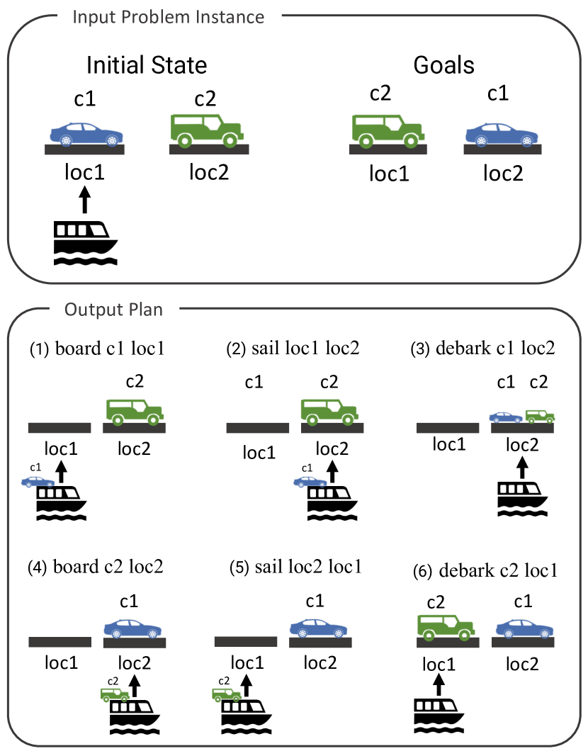
Figure 1: In the Ferry planning domain, an example of a problem instance involves an initial state comprising the location of a ferry and several cars, with specified goals for placing the cars in specific locations (top). The ferry is capable of boarding a car and transporting it between locations. The planning task entails generating a sequence of actions (i.e., a plan) such that executing them leads to reaching a goal state (bottom).

1 Introduction

Planning is a crucial aspect of artificial intelligence, which involves finding a sequence of actions that can achieve a specific goal in a given environment. Traditionally, planning problems are solved with graph-search heuristics which are based on solving relaxed problems (Blum and Furst, 1997; Hoffmann, 2001) or creating sub-goals by backtracking from the desired end-goals (Hoffmann et al., 2004; Helmert and Domshlak, 2009).

With the success of LLMs in various natural language processing tasks, there has been an increasing interest in utilizing them for applications that involve planning and reasoning, such as web agents (Yang et al., 2023; Yin et al., 2023; Huang et al., 2022), embodied agents (Huang et al., 2022; Song et al., 2023; Ahn et al., 2022) or open-world games (Wu et al., 2023; Wang et al., 2023). A compelling advantage of using Large Language Models (LLMs) for planning tasks lies in their ability to handle problems in natural language. This eliminates the need for formalizing them in strict languages like the Planning Domain Definition Language (PDDL; Malik Ghallab et al., 1998). However, LLMs have been found to lack the ability to solve classic planning tasks (Liu et al., 2023; Valmeekam et al., 2023a, b), and the magnitude of their failure in such tasks highlights the need for alternative approaches that can enhance their planning capabilities.

In our work, we start by examining whether LLMs possess capabilities that we deem as necessary for planning. We expand on the analyses of LLMs as planners done by Valmeekam et al. (2023b) and Silver et al. (2022), by focusing on specific capabilities that test their ability to comprehend diverse domains. Our analysis reveals limitations in the ability of LLMs to effectively model past actions and their subsequent impact on the current state. Additionally, the models struggle to identify the full spectrum of applicable actions and lack the capacity to prioritize sub-goals effectively, considering both necessary and optimal ordering. These findings highlight potential shortcomings in the planning and decision-making mechanisms employed by these models.

Motivated by our findings, we advocate for a hybrid methodology that integrates traditional planning algorithms with LLMs. We propose a similarity-based planner, $SimPlan$, a method which combines an action-ranking model with a greedy best-first search algorithm. This approach, as discussed in Section 4, addresses the shortcomings of LLMs described above and enhance the exploration of the state space. We evaluate our approach across various planning domains, comparing its efficacy with that of existing LLM-based planning strategies. The experiments reveal that our hybrid model surpasses traditional methods, underscoring the viability of combining LLMs with conventional planning techniques. We can summarize the contributions of our paper as follows:

• We evaluate LLMs shortcomings in reasoning about planning problems, underlying key missing capabilities.

• We introduce a new hybrid LLM-based planner that integrates classic planning algorithms and tools to overcome these limitations, $SimPlan$.

• We propose a novel generalized planning setup and demonstrate significant performance gains over prior work. However, the setup presents ongoing challenges.

The following sections are organized as follows. In Section 2, we provide a necessary overview of classic planning. Section 3 assesses the planning and reasoning capabilities of LLMs, evaluating their performance on various tasks. In Section 4, we introduce our novel approach, which leverages the strengths of traditional planning techniques to improve the efficiency of planning. Finally, in Section 5 we conduct experiments on several diverse planning domains, demonstrating the benefits of our hybrid approach.

2 Classical Planning

The core objective of a planning task is to construct a sequence of actions (i.e., a plan) that transitions from the initial state to a desired goal state. In classical planning, this process relies on a formal representation of the planning domain and the problem instance, encompassing the state space, actions, their preconditions and effects, and the desired goals. A widely used representation is the Planning Domain Definition Language (PDDL; Malik Ghallab et al., 1998). See Appendix A for more details about PDDL.

We now move to describe a problem instance within the Ferry planning domain as illustrated in Figure 1. This instance features a ferry and two cars, car1 and car2, initially positioned at separate docks, loc1 and loc2 respectively. The goal state is that car1 will be at loc2 and car2 will be at loc1. Each state is defined by the locations of the ferry and the cars (e.g., ferry is at loc1, car1 is at loc1, car2 is at loc2). Actions possess preconditions, outlining the state requirements for their execution, and effects, altering the state upon execution. For instance, the “board car1 loc1” action requires the ferry and car1 to be at loc1, and its execution results in car1 being on the ferry. The visualized plan involves six actions. Initially, “board car1 loc1” loads car1 onto the ferry. Then, “sail loc1 loc2” navigates the ferry to loc2. Subsequently, “debark car1” unloads car1 at loc2. Next, “board car2 loc2” loads car2, followed by “sail loc2 loc1” returning to loc1. Finally, “debark car2 loc1” unloads car2, achieving the goal.

Traditionally, classic planning problems have been solved using informed graph-search algorithms, such as greedy-best first search and the seminal A* algorithm (Doran and Michie, 1966; Richter and Westphal, 2010). To guide their search towards the goal state, these algorithms leverage several heuristics. Two prominent examples include the FF heuristic, known for its efficiency and scalability (Blum and Furst, 1997; Hoffmann, 2001), and the landmarks heuristic, which focuses on identifying critical states on the path to the goal (Hoffmann et al., 2004; Helmert and Domshlak, 2009).

Building on this, our work leverages generalized planning, a subfield of classical planning, as it offers a more apt framework for evaluating LLM capabilities. Within this paradigm, we learn a heuristic from training examples and subsequently assess its performance on a distinct set of instances, following the methodologies established by Yang et al. (2022); Silver et al. (2024). As detailed in Section 5, our evaluation hinges on a specific variant of generalized planning where the test set comprises problem instances exhibiting greater complexity compared to those in the training set.

Model grippers depots ferry minigrid blocks Falcon-180B $.11$ $.07$ $.45$ $.00$ $.24$ Mistral-7B $.00$ $.07$ $.31$ $.39$ $.16$ Mixtral-8x7B $.04$ $.14$ $.22$ $.35$ $.26$ LLama-2-70B $.60$ $.44$ $.50$ $.26$ $.52$ Codellama-34B $.01$ $.04$ $.43$ $.28$ $.14$ GPT-4 Turbo $.42$ $.26$ $.35$ $.59$ $.31$

Table 1: Success rates for describing the current state given an initial state and a sequence of executed actions.

Model grippers depots ferry minigrid blocks Falcon-180B $.63$ $.66$ $.68$ $.32$ $.57$ Mistral-7B $.30$ $.24$ $.41$ $.26$ $.18$ Mixtral-8x7B $.48$ $.51$ $.62$ $.41$ $.72$ LLama-2-70B $.60$ $.44$ $.50$ $.26$ $.52$ Codellama-34B $.64$ $.51$ $.61$ $.67$ $.43$ GPT-4 Turbo $.87$ $.84$ $.88$ $.86$ $.91$

Table 2: Success rates for predicting the applicable actions given a state.

3 The Shortcomings of LLMs as Planners

Several recent studies (Valmeekam et al., 2023a, b; Stein and Koller, 2023) have demonstrated limitations in the planning capabilities of LLMs. This section delves into these shortcomings, focusing on a targeted analysis of specific cognitive skills considered essential for successful planning. We start our evaluation by assessing the model’s capacity to grasp the operating principles governing the specific domain under consideration. These principles can be reasoned from the preconditions and effects associated with various actions. Next, we test the ability of LLMs to prioritize interim states required for achieving the goal states.

We evaluate the performance of various LLMs on these skills using an In-Context Learning approach (ICL). In particular, we test the following models: Falcon-180B (Almazrouei et al., 2023), Llama-2-70B (Touvron et al., 2023), Code-Llama-34B (Rozière et al., 2024), Mistral-7B (Jiang et al., 2023), Mixtral-8x7B (Jiang et al., 2024), and GPT-4 Turbo (OpenAI, 2023). The prompts for all the following experiments are provided in Appendix B. The examples for these experiments were randomly generated from diverse, well-known planning domains. Further details regarding the specific domains employed and implementation considerations are provided in Appendix C.

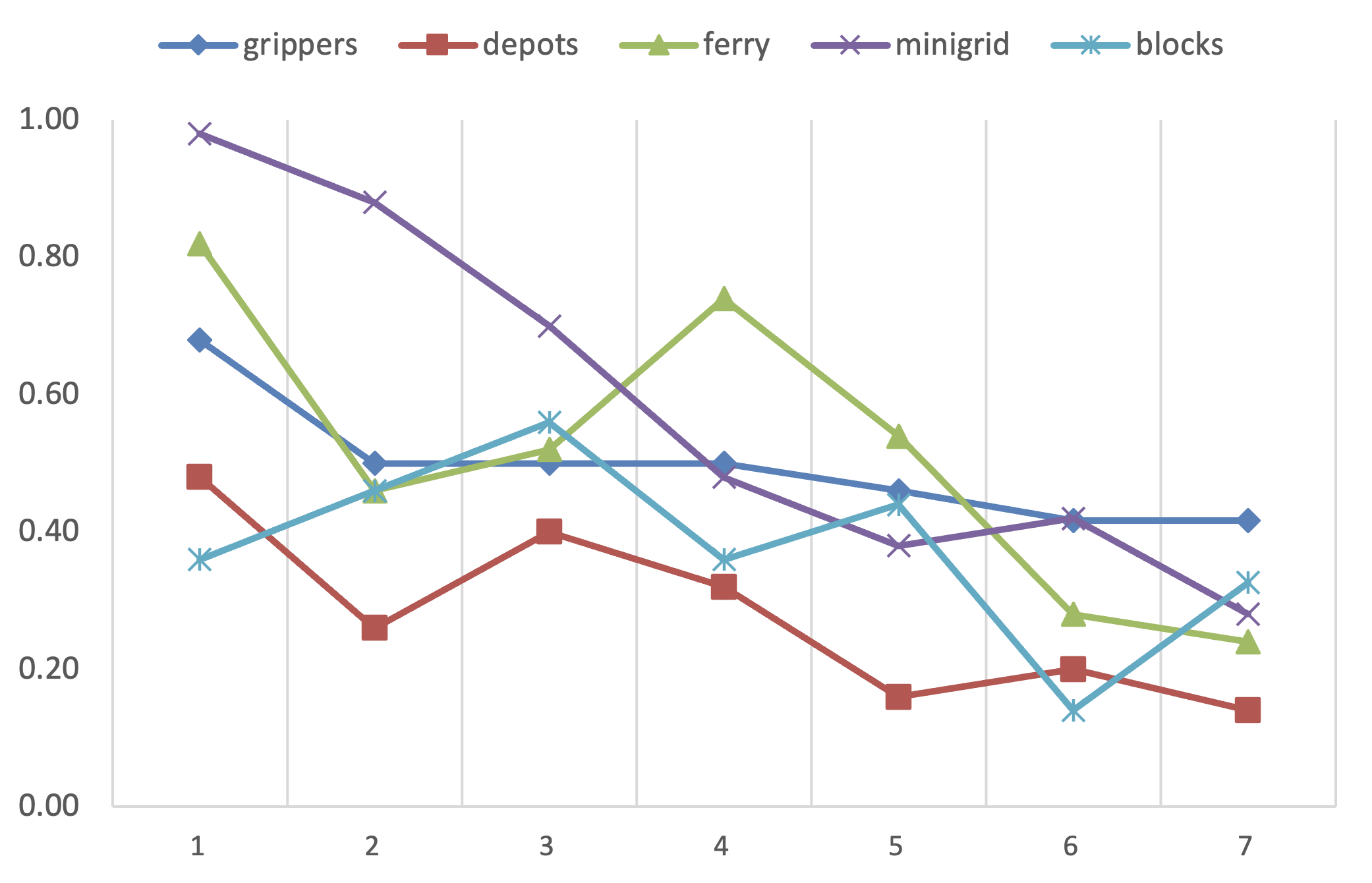
Figure 2: The maximum success rate across the different LLMs in inferring the new state, as a function of the number of actions taken.

3.1 Observation

The actions’ effects.

The model is given an initial state and a sequence of actions, and is asked to infer the new state after executing the sequence. This experiment was also conducted recently by Valmeekam et al. (2023b), however it was limited to a single domain and to GPT models.

The results of this experiment are demonstrated in Table 1. Overall we can observe that LLMs perform poorly in understanding how a sequence of actions affects the environment. Moreover, the results show that the models’ performance varies significantly depending on the complexity of the environment. For example, in the Minigrid environment, the Mistral-7B model performs poorly, with an accuracy of $0.14$. In contrast, the Falcon-180B model performs much better, with an accuracy of $0.21$. Moreover, we can observe that GPT-4-Turbo achieves the highest overall performance across all scenarios except Ferry, with percentages ranging from $30\%$ to $58\%$. Lastly, Figure 2 indicates that LLMs face increasing difficulty in accurately inferring the task state as the number of actions taken increases.

Applicable actions.

In this experiment, we evaluate the model’s understanding of the actions’ preconditions. This is done by providing the model with a state and a set of four possible actions and asking the model which action is applicable.

Table 2 presents the results of the applicable actions experiment. Although this task does not require complex reasoning abilities, the only model which exhibited consistently high accuracy across all evaluated environments is GPT-4 Turbo.

3.2 Goal Ordering

Reasonable and necessary ordering.

Within specific problem-solving domains, like Blocksworld and Minigrid, the sequential achievement of goals becomes critical due to the inherent dependencies between them. This necessitates the completion of certain goals prior to attempting others. For example, consider the Blocksworld domain where blocks are stacked on top of one another and at each step we can only remove the top block from each stack. Assume we are given the following goals: should be stacked on and should be stacked on . Within this scenario, prioritizing the completion of the latter goal would constitute a reasonable order. Otherwise, we would have to remove the blocks on top of before we can pick it up, and this would necessitate the destruction of the previously achieved goal.

Consider now the Minigrid domain, a domain where the agent has to pick-up keys and unlock doors in order to reach a certain location in a 2D map. We can observe that it is necessary to unlock some doors before others, since there are inner doors we can’t reach until we unlock the outer doors that are blocking the way. Accordingly, the ability of the model to prioritize goals in a reasonable and necessary fashion is crucial for planning, and has long been the subject of research in classical planning (Hoffmann and Koehler, 2000; Hoffmann et al., 2004).

Therefore, in this set of experiments, we present the model with two goals and ask it to choose which of the goals should be completed first. We choose to test this for the Blocksworld and Minigrid domains, since these domains require a reasonable or necessary order between the goals.

Optimal ordering.

In optimal planning, the current state imposes an ordering between the goals in order to avoid redundant actions. For example, in Figure 1, since the ferry is already at location 1, it should board car 1 so it can debark it at location 2, before moving to location 2. For this experiment we introduce a scenario where the model is provided with an initial state and a set of goals. The model then has to reason about which goal can be achieved with a lower number of actions. We use the Ferry and Grippers domains, as these domains do not have necessary or reasonable ordering between their goals. As such, the main consideration is the optimality of the plan.

The results for the goal planning experiments are presented in Table 3. Overall, Codellama-34B exhibits superior performance over the other models in 3 out-of 4 domains. However, in terms of adhering to optimal goal orderings, the models generally show similar performance, with scores ranging from $0.63$ to $0.67$. These findings suggest that models struggle with goal reasoning.

Reason. Neces. Optimal Model Blocks Minigrid Ferry Grippers Falcon-180B $.71$ $.69$ $.65$ $.65$ Mistral-7B $.58$ $.85$ $.63$ $.59$ Mixtral-8x7B $.04$ $.62$ $.64$ $.59$ Meta $.21$ $.69$ $.63$ $.59$ Codellama-34B $.13$ $.85$ $.67$ $.70$ GPT-4 Turbo $.75$ $.78$ $.63$ $.59$

Table 3: Success rate results for the goal planning experiments, testing for the model’s ability to prioritize goals when imposed with reasonable, necessary or optimal orderings.

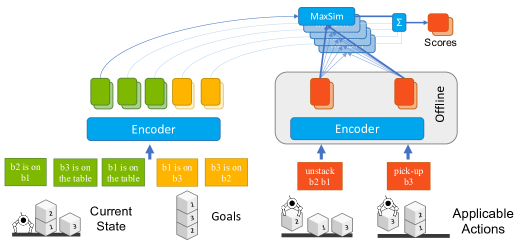
(a) The actions ranking model.

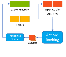
(b) The planning process.

Figure 3: Our proposed $SimPlan$ architecture. Colors green, yellow and orange are used to denote states, goals and actions, respectively. (a) At each iteration, a bi-encoder is used to generate contextualized token-level representations for the concatenated current state and goals, as well as for each applicable action. The actions’ representations can be extracted once in an offline process. Then, the set of applicable actions are ranked based on their similarity with the state and goals representation, using the late-interaction architecture of ColBERT (Khattab and Zaharia, 2020) (b) At inference time, the scores are inserted into a prioritized queue for choosing the next state.

4 SimPlan

In this section we present $SimPlan,$ an action-ranking model combined with a greedy best-first search (GBFS) algorithm designed to address the limitations observed in Section 3. First, We describe the data generation and augmentation process (Section 4.1). Next, we describe the architecture and the training process (Section 4.2). Finally, we discuss inference-time decoding (Section 4.3).

4.1 Data Generation and Augmentation

Planning problems formulation has a symbolic nature, which significantly simplifies training data generation. However, since this formulation uses unique identifiers for objects (e.g., blocks in Blockworld denoted as b1-b5), there is a potential bias risk. While seemingly arbitrary, these identifiers can inadvertently lead LLMs to develop preferences based solely on their frequency in the training data, To mitigate this issue, we augment the training dataset with 100 permutations per instance. These permutations involve replacing all objects indices with new sampled indices, essentially “de-identifying” the objects. This augmentation promotes LLM impartiality towards object indexing and enhances their ability to generalize to unseen indices during testing, resulting in a more robust and versatile model.

4.2 Learning to Rank Actions

This section introduces our action-ranking model, a bi-encoder model tasked with ranking applicable actions based on the current state and desired goals, as depicted in Figure 3a. Recognizing the inherent challenges faced by LLMs in generating applicable actions or even inferring what the applicable actions are, as observed in Section 3.1, we formulate the task of selecting the next action given a state and a goal as a retrieval problem. This retrieval-based approach ensures that the model only considers applicable actions.

Leveraging the late interaction architecture introduced by Khattab and Zaharia (2020), we propose an analogous schema wherein the goal and state serve as the query, while the action acts as the context. As illustrated in Figure 3a (top), this schema demonstrably enhanced predictive power by computing cosine similarity between individual tokens in the query and context, rather than relying on pooled representations. For each query token the maximum similarity score is selected, and the overall similarity score is calculated as the sum of these individual maxima. This similarity score can be regarded as the confidence of the model in the current path.

To optimize the model, we employ cross-entropy loss, comparing the top ranked action with the gold next action. To prevent the collapse of action representations where all actions become indistinguishable from each other, ranking actions based on their similarity requires the inclusion of negative examples during training. We employ two methods for incorporating negative examples to enhance model performance. Firstly, we leverage the in-batch negative sampling approach described by Henderson et al. (2017). Within each training batch containing $n$ action-state pairs, every other pair serves as a negative example for every original pair. Secondly, we create “hard negative” examples using three distinct techniques: (1) action name replacement, where actions are swapped (e.g., changing the action “debark car1 loc1” to the opposite action “board car1 loc1”); (2) subterm swapping, where the order of subterms is changed (e.g., changing “sail loc1 loc2” to “sail loc2 loc1”); and (3) random subterm sampling, where individual subterms are replaced with random values (e.g., changing “board car2 loc2” to “board car1 loc1”). These techniques ensure the generated negatives are syntactically similar to the positive examples, forcing the model to learn finer distinctions between actions.

4.3 Planning

Our proposed planning approach addresses two key challenges described earlier: (1) the negative correlation between the number of executed actions and the accuracy of describing the current state; and (2) the limitations of beam search used by LLMs for planning tasks.

State Updates.

In Section 3.1 we demonstrated a negative correlation between the number of actions taken and the accuracy of a large language model (LLM) in describing the current state. To circumvent this issue and align with the methodology employed in Hao et al. (2023), we adopt a state-update strategy that calculates the new state directly from the current state and the chosen action, bypassing the LLM’s potentially inaccurate inference.

Greedy Best-First Search Algorithm.

The common decoding algorithm used for natural language generation is the beam search algorithm, which is a local search algorithm that keeps only a fixed number $k$ of promising paths as candidates. While effective for optimization problems, the beam search algorithm has several limitations related to planning problems. First, a known issue associated with beam search is that it “can suffer from a lack of diversity among the $k$ paths–they can quickly become concentrated in a small region of the search space” (Russell and Norvig, 2009). Second, unless they are implemented with backtracking, local search algorithms lack the ability to continue from an earlier generated path and explore taking alternative actions. Drawing inspiration from well-known classic planners (e.g., the LAMA planner (Richter and Westphal, 2010)), we employ a graph-based algorithm to address this limitation. GBFS chooses the next node to expand based on a cost function. Similar to the implementation of beam search for language generation, our cost function is implemented as an aggregated score of all the probabilities extracted for actions participating in the path. However, to avoid penalizing long sequences, we replace the sum log probability with an average log probability. Overall, we suggest that GBFS will facilitate greater exploration of high-potential paths, making it better suited for goal-directed planning.

We now describe the planning process of our approach, as depicted in Figure 3(b). We implement the GBFS algorithm using a priority queue, which is intended to manage all explored states and prioritize their subsequent expansion. We limit the queue size to $1000$ to avoid incurring memory issues. We start by generating and encoding all applicable actions using the trained bi-encoder and store their representations in memory. Afterwards, the initial state is added to the priority queue. At each step, the state with the highest priority, alongside the goals predicates, is encoded using the trained bi-encoder to extract its latent tokens representation. Similarity scores are extracted by comparing the state’s latent tokens representation with all applicable actions, as described in Section 4.2. Using the acquired scores, a heuristic value is calculated for each explored path. This iterative process continues until the desired goal state is reached.

Blocks Ferry Grippers Depots Minigrid Method S C S C S C S C S C LLM4PDDL GPT-4 Turbo (no validation) .26 .0 .20 .0 .60 .0 .30 .0 .13 .08 LLM4PDDL CodeLlama-34b-instruct .07 .0 .25 .0 .33 .0 .03 .0 .07 .0 Plansformer CodeLlama-7b-instruct .96 .0 .80 .0 .90 .0 .53 .0 .93 .88 Random .33 .0 .03 .0 .20 .0 .13 .0 .16 .22 # Goals Completed Heuristic .25 .0 .63 1.0 .76 .96 .43 .0 .16 .22 $SimPlan$ (ours) 1.0 .56 1.0 1.0 1.0 1.0 1.0 .12 1.0 .86

Table 4: The fraction of test problems solved. We report the results both on a test set of simple problem instances (S), which have the same configuration as the problems used in the training set, and complex problem instances (C) with an increased number of objects. The bolded results are significant (paired student’s t-test, $p<0.05$).

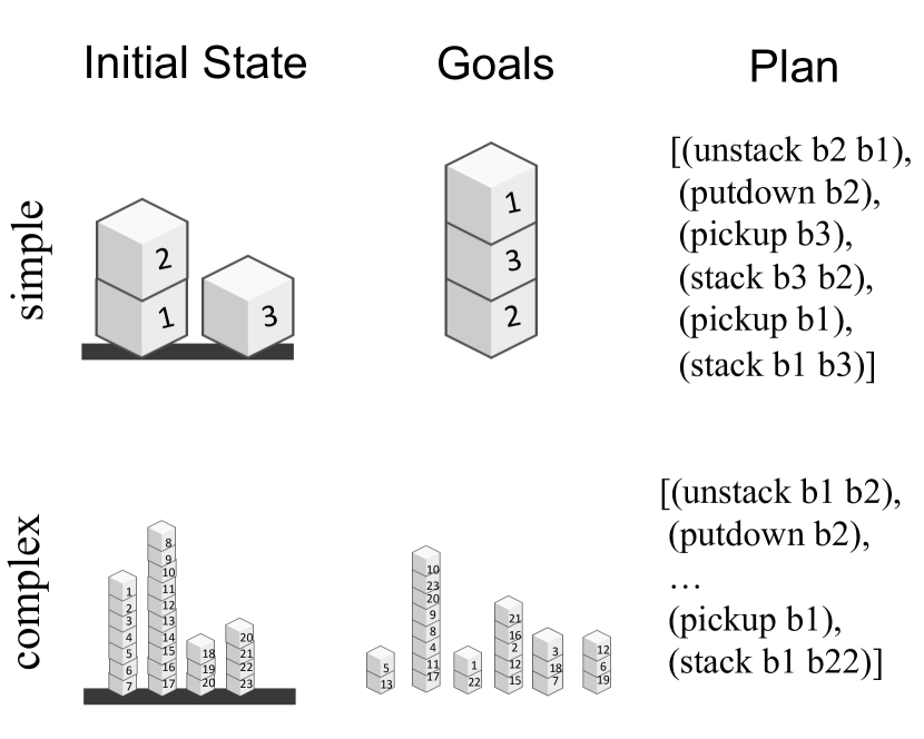
Figure 4: An example of our experimental setting for the Blocksworld domain. The train and development sets include problem instances from a simple configuration (top), and the test set include problem instances from a complex configuration (bottom), where the difference between the two configurations is the number of blocks.

5 Experiments

To assess the effectiveness of our proposed method, we conduct experiments testing the capability of the $SimPlan$ algorithm to generalize from simplified tasks to more complex scenarios, as demonstrated in Figure 4. The domains used in the experiments were the ones covered in Section 3.

5.1 Datasets

To systematically evaluate planning model performance across varying difficulties, we generated two problem configurations for each domain: simple and complex. The configurations vary in their number of objects. For example, in Blocksworld, simple configurations consists of 2-5 blocks, while complex configurations featured 11-25 blocks. Each instance includes a plan generated by the LAMA planner (Richter and Westphal, 2010) for training purposes.

This manipulation impacts plan length in two key ways: (1) More objects introduce more goals, and (2) new objects can act as obstacles, requiring further actions for removal. For example, in Blocksworld (Figure 4), stacking a new atop require two additional actions to remove it before unstacking from . In addition, a new goal can be added, such as placing on top of , which would require two additional steps to pick it up and stack it, totaling in increasing the plan length by four actions. Consequently, simple problems had an average plan length of $13.5$ actions, while complex problems had a significantly higher average of $357.2$ actions. More details about the datasets can be found in Appendix C.

5.2 Baselines

The baselines used in our experiments can be categorized as follows:

1. In-context Learning: The first baseline utilizes vanilla GPT-4 Turbo and directly instructs it to generate a plan. The second baseline incorporates CodeLlama-34b-instruct with a soft-validation strategy to address poorly formatted LLM outputs. Both adhere to the two-example few-shot prompt design established by LLM4PDDL (Silver et al., 2022).

2. Fine-tuning: Code-llama-7b-instruct model, trained for code instruction tasks, was fine-tuned using the approach proposed by Plansformer (Pallagani et al., 2022).

3. Naive Baselines: We added two naive approaches: (1) Random, samples a subsequent action from a list of applicable actions; and (2) # Goals Completed Heuristic, a GBFS with a heuristic considering the number of fulfilled goals.

Experimental Setup.

All models are trained using instances from the simple configuration and are then tested separately on unseen instances from the simple and complex configurations. In order to produce comparable results we set a fixed number of next action predictions for each problem instance based on the number of states that a classic planner expanded, further elaborated in Section D.2. Following Valmeekam et al. (2023b), we measured the model’s ratio of solved problems instances.

5.3 Results

The performance of the different baselines and $SimPlan$ is presented in Table 4. First we can observe that $SimPlan$ surpasses all other models across all problems and configurations except for comparable results on the complex configuration in Minigrid. Moreover, we can observe that all models struggled in the challenging Depots domain. This domain necessitates object stacking (akin to Blocksworld) while introducing the requirement of object relocation (similar to Ferry). This combination leads to actions with many subterms (e.g., unload hoist3 crate14 truck0 distributor1) and difficult reasoning challenges.

As anticipated and aligned with the expectations established in Section 3, LLM-based baseline planners struggle in tackling complex problem instances. This finding diverges from the results reported by LLM4PDDL (Silver et al., 2022), which demonstrated strong generalization capabilities within the Grippers domain. We believe that this discrepancy is attributed to the increased complexity of our Grippers setup, featuring five rooms compared to the two employed in LLM4PDDL (see Appendix C).

The Random model’s similar performance across simple and complex Minigrid tasks suggests minimal complexity increase, suggesting a possible explanation to Plansformer’s performance in this domain. The # Goals Completed baseline exhibits strong performance in Ferry and Grippers domains, highlighting the potential benefits of a simple goal counting heuristic in specific domains, particularly in the domains where the goals are independent. Conversely, the Blocksworld domain favors the Random baseline over the goal-oriented approach, underscoring the critical role of goal ordering in effective planning.

Method Blocks Ferry Minigrid $SimPlan$ .56 1.0 .86    w/o Hard Negatives .36 1.0 .78    w/o Data Augmentation .0 .0 .56    w/o Updating State .0 .0 .64

Table 5: Ablation results, reporting the fraction of test problems solved from the complex configuration.

5.4 Ablations

We conducted an ablation study analyzing the contributions of various components in our $SimPlan$. We evaluated the contributions of hard negatives, data augmentation and the state updates component. See Appendix E for implementation details.

The results are presented in Table 5. We can observe that hard negatives provided a significant improvement in the results. Data augmentation, however, was crucial for generalization, as its removal hindered handling previously unseen objects indices. Finally, eliminating state updates led to poor performance, highlighting the difficulty for LLMs to manage state solely through action sequences.

6 Related work

Valmeekam et al. (2023b) presented a benchmark for evaluating LLM-based planners and concluded that such models display subpar performance. Follow-up works suggested enriching the planning process with multiple reasoning steps inspired by Chain-of-Thought and Tree of Thoughts (Wei et al., 2022; Yao et al., 2023). Hu et al. (2023); Stein and Koller (2023) prompt the LLM to reason how the goals can be achieved before generating a plan. Hao et al. (2023) prompt the LLM to describe the updated state between each executed action. Valmeekam et al. (2023c) proposed that models will self-critique their own generated plan and fix them, similar to (Madaan et al., 2023). However, many of these works concluded that models tend to struggle with such reasoning tasks. Our analysis in Section 3 is motivated by this line of research, underlying missing reasoning capabilities in LLM-based planners.

Recognizing LLMs’ limitations, follow up work explored hybrid approaches of using LLMs along with classic planning tools. Valmeekam et al. (2023c) tested the use of a planning verification tool instead of LLM to provide feedback for generated plans. Silver et al. (2022) also used a planning verification tool to find and fix inapplicable actions, as described in Section 5. Pallagani et al. (2022) used a classic planner to generate a large training dataset of solved problems in order to fine-tune code models for planning. Our work follows this hybrid approach, assuming access to planning tools (Section 4). However, we diverge in the experimental setup (Section 5) by focusing on generalized planning. In other words, we examine how models cope with significantly larger problems than seen during fine-tuning, a novel aspect compared to prior works.

7 Conclusions

Despite the encouraging outcomes achieved by our approach, a notable gap exists between the efficency of traditional planners and LLM-based planners. We aim to narrow this gap by exploring new hybrid techniques, particularly focusing on areas such as goal ordering where the LLM exhibited poor performance in our evaluations. In future work, we intend to broaden the scope of our methodology to address real-world planning challenges that deviate from the structured PDDL format, including scenarios relevant to web and embodied agents. Through these efforts, we aim not only to refine the efficacy of our methodology but also to extend its utility across a more diverse array of planning tasks. To facilitate these advancements, we advocate for the employment of our dataset as a robust platform for testing planning algorithms.

Limitations

Classic planning problems have been developed for over two decades and include many domains and variants of planning, such as numeric planning and optimal planning. Our work focuses on 5 domains which we found interesting, such as a navigation task, and a domain which combines the challenges from two other domains in our set (Depots). However, this work is not an exhaustive evaluation of LLM-based planners. Regarding $SimPlan$, as described in the paper, we found that it degrades in performance as we add more objects in Blocksworld, which indicates a weakness when adding more blocks with dependencies amongst them. In addition, our approach is limited by the max sequence length of the LLM, which would make it difficult to handle significantly larger problems.

Ethics

This paper presents work whose goal is to advance the field of Machine Learning. There are many potential societal consequences of our work, none which we feel must be specifically highlighted here.

basicstyle=,xrightmargin=1.5em, showstringspaces=false, showspaces=false, showtabs=false, tabsize=2, breaklines=true, flexiblecolumns=true, escapeinside=<@@>, breakatwhitespace=true

Appendix A PDDL

Figure 5: An example PDDL problem instance definition for the Ferry domain.

Figure 6: The PDDL Ferry domain definition. The domain definition specifies the predicates and actions, encapsulating the physics of the domain.

Classical planning is based on the notion that the entire planning domain and problem instance are described in a formalised, machine-readable format. One common format is the Planning Domain Definition Language (PDDL; Malik Ghallab et al., 1998). The domain definition (Figure 6) encodes the physics of the world, while the problem instance definition (Figure 5) specifies the initial state and desired goals, thereby customizing the domain to a specific scenario. The planning task entails generating a sequence of actions that facilitate a transition from the initial state to a goal state, thereby constituting a plan.

A domain consists of a pair <P,A>, where P represents a set of predicates, and A is a set of actions. Each predicate $p\in{P}$ includes a name and a set of variables denoted by a question mark. For instance, at-ferry ?l is a predicate, while at-ferry(loc1) is a specific truth-assignment to the predicate, indicating the ferry’s presence at location 1. Predicates can also be negated (e.g., not(at-ferry(loc1))). An action $a\in{A}$ consists of a name, a set of variables, a set of effect predicates, and a set of precondition predicates. For instance, board(?car ?loc) is an action denoting the boarding of car ?car on the ferry at location ?loc. The action’s preconditions include predicates such as at_ferry(?loc), at(?car,?loc), and empty_ferry, signifying that both the ferry and the car ?car are at location ?loc, and that the ferry is empty. The action’s effects include predicates such as not(empty_ferry), not(at(?car,?loc)), and on(?car), indicating that the ferry is no longer empty, that the car ?car is no longer at location ?loc, and that the car ?car is now on the ferry.

A problem is a triple <O,I,G>, where O is a set of objects, I is a set of truth-assigned predicates that are currently true in the world model, and G is a set of truth-assigned predicates designated to be achieved.

Appendix B Shortcomings of LLMs Experiment Details

In Section 3 we described a set of controlled experiments which test for specific reasoning abilities of LLM-based planners. Our prompt is constructed as following: for each domain we start by describing the domain, such as exemplified by Figure 7. Then, using the relevant prompt for each experiment (Figures 8, 9, 10 and 11), we add 2 example questions which contain an answer, followed by an unsolved example.

Figure 7: Explanation provided about the Blocksworld domain before each Blocksworld experiment described in Section 3.

Figure 8: Prompt template used for the actions’ effects experiment.

Figure 9: Prompt template used for the applicable actions experiment.

Figure 10: Prompt template used for the optimal goals ordering experiment.

Figure 11: Prompt template used for the reasonable or necessary goals ordering experiment.

Blocks Ferry Grippers Depots Minigrid Simple Complex Simple Complex Simple Complex Simple Complex Simple Complex # Objects 2-5 11-25 2-5 11-25 2-5 11-25 2-5 11-15 1-2 3-8 Avg. plan length 8.3 88.5 11.3 50.2 10.1 52.5 10.4 132.1 19.5 27.3 Changed Object Blocks Cars Balls Crates Shapes

Table 6: Changes in the number of objects and average plan lengths between the simple and complex configurations.

Simple Complex Train Dev Test Test 100 30 30 50

Table 7: The size of the sets generated for each domain.

Appendix C Generating Problem Instances and Plans

In this section we provide more details about the generated problem instances and the plans to solve them. We start by generating problem instances with the PDDL generators library (Seipp et al., 2022), which we use to generate our experiments’ data, as described in Section 3, as well as the training, validation and test datasets, as described in Section 5. When generating problems, the amount of objects for each generated problem instance is controllable. For example, the Grippers domain problem generator configuration controls the amount of robots, balls and rooms. For each domain, we choose one object to tweak its amount, and fix the amount of all other objects. For example, in the Grippers domain we only change the number of balls, and we fix the number of robots to 1 and the number of rooms to 5. We then increase the number of instances of that object between the simple and complex configurations to create longer plans. The configurations used are described in Table 6 and the size of the datasets is described in Table 7. An example of a complex configuration plan is provided in Figure 18 to illustrate the difficulty of the task.

We then solve the generated problem instances with the LAMA planner and save the found plans. Lastly, we remove problem instances based on the following filters:

• Timeout or search unsolved: Problem instances that the LAMA planner could not solve after a ten-minute timeout or after exploring the entire search space were removed. If there were many such errors, we tweaked the configurations such that the LAMA planner can solve the problems, until we reached the configurations described in Table 6.

• Empty plans: Instances where their plans have no steps were removed. This can happen in cases where the initial state is a goal state.

• Duplicates: Instances with the same initial state and goals are removed.

C.1 Domains

Blocksworld.

In this domain, the objects are blocks and the agent is a robotic arm that can pick them up and put them down on a table. Blocks can be stacked, and only a block that is clear (i.e., doesn’t have a block on top of it) can be picked up. The goal predicates are to stack blocks on top of other blocks.

Ferry.

In this domain the objects are cars and locations, and the agent is a ferry that can move between locations, board a car in one location or debark it in another location. The ferry can only board one car at a time. The problem requires the ferry to transport the cars to their designated locations.

Grippers.

In this domain the objects are balls and rooms, and the agent is a robot that can move between rooms, pick-up balls or drop a picked-up ball. The robot can hold two balls simultaneously with its left and right grippers. The problem requires the robot to transport the balls to their designated rooms.

Depots.

Similar to Blocksworld, the objects are crates and the agent is a hoist that can pick them up or put them down. The difference from Blocksworld is that there are multiple “tables”, which are called pallets, and each pallet has its own hoist. The pallets are located in different locations, called depots and distributors. The truck is another agent that can move the crates between locations. This is similar to Ferry and Grippers. The goal predicates are to stack the crates at specific locations, or on top of other crates.

Minigrid.

In this grid domain, the objects are walls, keys and doors, and the agent is a robot that can traverse the grid, pick up keys and unlock doors. Doors can be locked, and their locks have certain shapes with keys having matching shapes. Only one key can be picked up at a time, thus the robot must first drop a key in order to pick up a different key. The more number of shapes there are, the more often the robot has to switch the key it is holding. The goal predicate is to reach a certain location in the board. The floor plan that we used for all Minigrid problems is depicted in Figure 12.

C.2 Domains Modifications

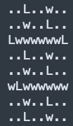
Figure 12: Minigrid floorplan that we used for generating problem instances. L represents locked doors, w represents blocked places which can’t be crossed, and all other dots represent places where the agent can walk. In each problem instance, the robot start and end location are chosen randomly. The keys are spread around the map, not depicted in this figure.

Some domains have a lot of predicates to describe the current state, thus creating a very long prompt for the LLM. This is a problem mostly in the Minigrid domain, which as seen in Figure 12, has a large 2D map which contains 64 places. This map is meticulously described in the PDDL format. To sidestep this problem of having extremely long prompts, we make several changes to their PDDL definition which allow us to create a shorter state representation. Firstly, we remove predicates that contain typing information of objects. For example, we remove predicates that mention that the object p1 is a place (place p1), that the object key1 is a key (key key1), and that the object shape1 is a shape (shape shape1). Given this change, it should still be possible to calculate applicable actions, as LLMs have different representations for each token, and they can infer the type of the object from the prefix, context and provided examples. In addition, we remove predicates which contain information about connected paths, such as p1 is connected to p2 (conn p1 p2). Originally, this is used in Minigird to represent the locations of walls. We remove this only for the fine-tuned models which can learn the map during training. Finally, in Minigrid, we remove predicates which indicate that a door is open (e.g., open p3). The predicates already describe which doors are locked (e.g., locked p16), and it should be possible for the LLM to see which places are locked and from it to infer the open doors.

C.3 Goal Planning Experiment

As described in Section 3.2, we devise experiments in which there is one goal that should reasonably or necessarily be prioritized over a different goal. To identify such instances, we employ the landmarks graph generated by the LAMA planner (Richter and Westphal, 2010). Landmarks are sub-goals that the LAMA planner algorithm identified as necessary to complete in any possible plan that solves the given problem instance. This graph’s nodes represent goals or intermediate sub-goals, with directed edges denoting the order in which these goals should be approached. The edges are labeled to indicate the type of ordering, such as “n” for necessary and “r” for reasonable. Utilizing these labels, we construct prompts for the language model that requires prioritizing between 2 distinct goals, as described in Appendix B. In the context of the Blocksworld domain, our selection criteria for goals involve choosing those linked by a minimum of two edges, ensuring that the same block does not appear in both goals.

Appendix D Training Details

This section provides further details about the training of our $SimPlan$ model and the baselines.

D.1 Approaches

SimPlan.

We start by reporting results for our similarity-based retrieval model, $SimPlan$. For evaluating the retrieval model, we use the metric MAP@100. The performance of the retrieval model on the intrinsic development set (comprised of simple difficulty problems) ranges from 60% to 90% between domains. For all domains we used a batch size of 32, except for the Depots and Minigrid domains which we used a batch size of 16. Then, an extra 2 hard negatives are added per example in the batch, sampled from the pool of hard negatives which was extracted using the techniques described in Section 4.2. We used one A100 80-GB GPU to train each model for 10 epochs with a training time of 12 hours, and selected the best checkpoint. For hyperparameter tuning we used a grid search with the following parameters: learning rate varied between [4e-5, 4e-4, 4e-3], warmup steps varied between [0, 100, 500] and weight decay varied between [0.01, 0.001, 0.0001]. After hyperparameter tuning, we fixed the parameters to a learning rate of 4e-4, warmup steps of 100 and a weight decay of 0.001. Our implementation is based on the sentence transformers library adapted with code from the ColBERT library. We implemented our own simple planning translator based on the PDDL domains definitions. See Figure 14 for an example input / output.

LLM4PDDL.

Our first two baselines are based on the in-context learning approach, for which we follow the few-shot prompt design from LLM4PDDL (Silver et al., 2022) with 2 training examples. See Figure 15 for an example prompt. For GPT-4 Turbo, we use the vanilla strategy where we simply prompt the model to generate a plan with temperature 1.0. For CodeLlama-34b-instruct, we use the soft-validation strategy for dealing with malformed LLM outputs. In the soft-validation strategy, a planning translator is used to find all applicable actions at each step. After each action is generated, it is validated that it is applicable in the current state. If it is not, it is replaced with the closest valid action, based on a cosine similarity distance in a pre-trained embedding space of the paraphrase-MiniLM-L6-v2 model. For CodeLlama-34b-instruct, we use a beam size of 1, similar to LLM4PDDL. To allow more exploration of the search space, we sample 16 different plans from the LLM with a temperature of 0.5.

Plansformer.

We fine-tune an LLM on the training set of problem instances from the simple configuration. The following fine-tuning settings described is based on Pallagani et al. (2022). We use CodaLlama-7b as the base model, which follows the intuition by Plansformer to use code models. The input to the model contains the initial state and the goals, along with the description of the domain’s actions. We add special tokens between the different parts, such as <GOAL>, <INIT>, <ACTION>, <PRE>, <EFFECT> to describe the goals, the initial state, and the actions, along with their preconditions and effects. The gold output is a sequence of actions which make up a plan. See Figure 13 for an example of an input / output. For early stopping, we use Rouge-L to compare the gold output with the predicted output on a development set of easy problems. During generation, we use a beam search of 16 to allow for a large exploration of the state space.

Figure 13: Example $SimPlan$ state parsed and linearized into tokens. During training, for each problem instance the blocks names are scrambled in order for the model to train the embeddings of all relevant tokens. In this example, b2 was converted into b24.

Figure 14: Example Plansformer instance.

Figure 15: Example LLM4PDDL baseline prompt for a Blocksworld problem instance prepended with two training examples. This format is based on Silver et al. (2022), where newlines separating the predicates were replaced with spaces in this figure for the sake of brevity.

D.2 Inference-time constraints

To produce comparable results between the different models, for each model we limit the number of next actions predictions. For $SimPlan$ and the random baseline, the number of predictions is simply the count of calls to the model, since we predict one next action in each model call. For LLM4PDDL and Plansformer, after each token is generated, we implemented a check if this token is one of the following tokens: ")" or "),(". If yes, we identify this as a generated action and count this as one prediction. An important aspect of beam search is that each beam generating an action increases this count by one. A stop criteria is applied once the number of predictions exceeds the limitation. We note that this limitation is not implemented for GPT-4, as the amount of beams that GPT-4 uses is not information that we found available.

The value of the limit for next action predictions is configured differently per problem instance. We first calculate how many states were expanded by the LAMA planner when solving each problem instance. However, since the LAMA planner uses greedy best-first search, it is not limited to sequential exploration like beam search. It is thus possible that this limitation is too harsh for beam-search decoding algorithms which sequentially extract multiple paths, reducing the overall maximum explored plan length. We thus multiply this limitation by 16, which is the beam size we used for beam-search decoding algorithms. Finally, we also set a timeout of 5 minutes for all models.

Appendix E Ablation Experiment Details

In this section we provide more information about the ablation experiments in Section 5.4, specifically about the state updates experiment. As mentioned in Section 4.3, our $SimPlan$ method involves updating the state at each step, and the history of the actions taken is not included in the input to the encoder. For the state updates experiment, we train a variant of our model where the input to the model is fixed to the initial state as defined in the problem instance, the set of goals, and the sequence of actions taken so far. Special tokens are used to separate between the state predicates, goal predicates and the actions. The model is then expected to infer the current state based on the initial state and the sequence of actions, similar to the LLM4PDDL and Plansformer baselines.

Appendix F Learned Representation Analysis

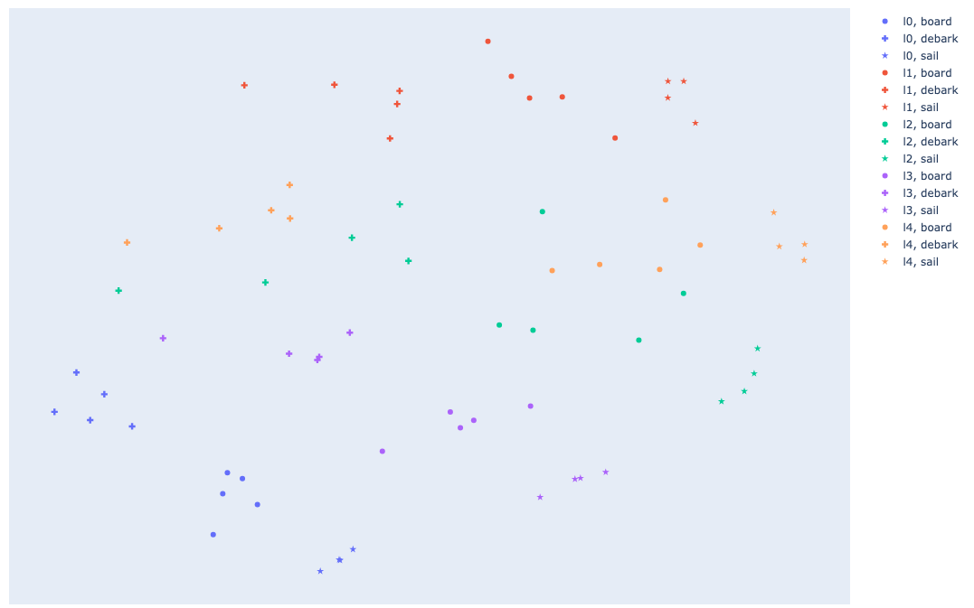
Figure 16: T-SNE plot of the learned representation of actions in the Ferry domain. The shapes depict the different action types, and the colors depict the different locations where the ferry is at when taking the action. The visible clusters of colors indicate that the model learned the concept of applicable actions.

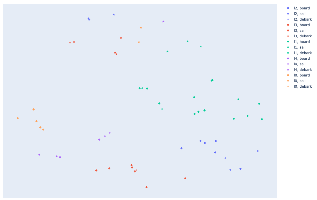
Figure 17: T-SNE plot of the learned representation of sampled states in the Ferry domain. Colors and shapes are determined based on the next action to take in this state according to the gold plan. The visible clusters of color-shape pairs indicate that the model is taking goal-informed decisions when representing the current state.

We analyze the learned representation of the actions and the states, described in Section 4, by using the T-SNE algorithm (Figures 16 and 17). Since we are using a late interaction schema, each individual state or action representation has multiple token embeddings. For our analysis, we chose to take the maximum token embedding. To create states to use for our analysis, we sampled 5 problem instances from our training dataset and extracted a state after the execution of each action in the accompanied plan. In the visualization, each state is assigned an action based on the next action in the plan.

The figures in our analysis show that the model learns the concept of applicable actions and next action planning. In our settings of the Ferry domain, there are overall 5 locations. In the actions representations (Figure 16), the colors represent the location of the ferry. Since the colors are well-clustered, and the location of the ferry determines the applicable actions, this demonstrates that the model learned the concept of applicable actions. In addition, in the states representations visualization (Figure 17), we can see that different states which have similar next actions are clustered together. This demonstrates that the action-ranking model is taking goal-informed decisions. Interestingly, in the states representation, the model clusters together the debark actions (star shape).

basicstyle=,breaklines=true

Figure 18: Example plan with 204 actions for a problem instance from the Blocksworld’ complex configuration.

References

- Ahn et al. (2022) Michael Ahn, Anthony Brohan, Noah Brown, Yevgen Chebotar, Omar Cortes, Byron David, Chelsea Finn, Chuyuan Fu, Keerthana Gopalakrishnan, Karol Hausman, Alex Herzog, Daniel Ho, Jasmine Hsu, Julian Ibarz, Brian Ichter, Alex Irpan, Eric Jang, Rosario Jauregui Ruano, Kyle Jeffrey, Sally Jesmonth, Nikhil J. Joshi, Ryan Julian, Dmitry Kalashnikov, Yuheng Kuang, Kuang-Huei Lee, Sergey Levine, Yao Lu, Linda Luu, Carolina Parada, Peter Pastor, Jornell Quiambao, Kanishka Rao, Jarek Rettinghouse, Diego Reyes, Pierre Sermanet, Nicolas Sievers, Clayton Tan, Alexander Toshev, Vincent Vanhoucke, Fei Xia, Ted Xiao, Peng Xu, Sichun Xu, Mengyuan Yan, and Andy Zeng. 2022. Do As I Can, Not As I Say: Grounding Language in Robotic Affordances.
- Almazrouei et al. (2023) Ebtesam Almazrouei, Hamza Alobeidli, Abdulaziz Alshamsi, Alessandro Cappelli, Ruxandra Cojocaru, Mérouane Debbah, Étienne Goffinet, Daniel Hesslow, Julien Launay, Quentin Malartic, Daniele Mazzotta, Badreddine Noune, Baptiste Pannier, and Guilherme Penedo. 2023. The falcon series of open language models.
- Blum and Furst (1997) Avrim L Blum and Merrick L Furst. 1997. Fast Planning Through Planning Graph Analysis.
- Doran and Michie (1966) James E Doran and Donald Michie. 1966. Experiments with the graph traverser program. Proceedings of the Royal Society of London. Series A. Mathematical and Physical Sciences, 294(1437):235–259.
- Hao et al. (2023) Shibo Hao, Yi Gu, Haodi Ma, Joshua Jiahua Hong, Zhen Wang, Daisy Zhe Wang, and Zhiting Hu. 2023. Reasoning with Language Model is Planning with World Model.
- Helmert and Domshlak (2009) Malte Helmert and Carmel Domshlak. 2009. Landmarks, Critical Paths and Abstractions: What’s the Difference Anyway? Proceedings of the International Conference on Automated Planning and Scheduling, 19:162–169.
- Henderson et al. (2017) Matthew Henderson, Rami Al-Rfou, Brian Strope, Yun-hsuan Sung, Laszlo Lukacs, Ruiqi Guo, Sanjiv Kumar, Balint Miklos, and Ray Kurzweil. 2017. Efficient Natural Language Response Suggestion for Smart Reply.
- Hoffmann and Koehler (2000) J. Hoffmann and J. Koehler. 2000. On Reasonable and Forced Goal Orderings and their Use in an Agenda-Driven Planning Algorithm. Journal of Artificial Intelligence Research, 12:338–386.
- Hoffmann et al. (2004) J. Hoffmann, J. Porteous, and L. Sebastia. 2004. Ordered Landmarks in Planning. Journal of Artificial Intelligence Research, 22:215–278.
- Hoffmann (2001) Joerg Hoffmann. 2001. FF: The Fast-Forward Planning System. AI Magazine, 22(3):57–57.
- Hu et al. (2023) Hanxu Hu, Hongyuan Lu, Huajian Zhang, Yun-Ze Song, Wai Lam, and Yue Zhang. 2023. Chain-of-symbol prompting elicits planning in large langauge models.
- Huang et al. (2022) Wenlong Huang, Pieter Abbeel, Deepak Pathak, and Igor Mordatch. 2022. Language Models as Zero-Shot Planners: Extracting Actionable Knowledge for Embodied Agents.
- Jiang et al. (2023) Albert Q. Jiang, Alexandre Sablayrolles, Arthur Mensch, Chris Bamford, Devendra Singh Chaplot, Diego de las Casas, Florian Bressand, Gianna Lengyel, Guillaume Lample, Lucile Saulnier, Lélio Renard Lavaud, Marie-Anne Lachaux, Pierre Stock, Teven Le Scao, Thibaut Lavril, Thomas Wang, Timothée Lacroix, and William El Sayed. 2023. Mistral 7b.
- Jiang et al. (2024) Albert Q. Jiang, Alexandre Sablayrolles, Antoine Roux, Arthur Mensch, Blanche Savary, Chris Bamford, Devendra Singh Chaplot, Diego de las Casas, Emma Bou Hanna, Florian Bressand, Gianna Lengyel, Guillaume Bour, Guillaume Lample, Lélio Renard Lavaud, Lucile Saulnier, Marie-Anne Lachaux, Pierre Stock, Sandeep Subramanian, Sophia Yang, Szymon Antoniak, Teven Le Scao, Théophile Gervet, Thibaut Lavril, Thomas Wang, Timothée Lacroix, and William El Sayed. 2024. Mixtral of experts.
- Khattab and Zaharia (2020) Omar Khattab and Matei Zaharia. 2020. Colbert: Efficient and effective passage search via contextualized late interaction over bert.
- Liu et al. (2023) Bo Liu, Yuqian Jiang, Xiaohan Zhang, Qiang Liu, Shiqi Zhang, Joydeep Biswas, and Peter Stone. 2023. LLM+P: Empowering Large Language Models with Optimal Planning Proficiency.
- Madaan et al. (2023) Aman Madaan, Niket Tandon, Prakhar Gupta, Skyler Hallinan, Luyu Gao, Sarah Wiegreffe, Uri Alon, Nouha Dziri, Shrimai Prabhumoye, Yiming Yang, Shashank Gupta, Bodhisattwa Prasad Majumder, Katherine Hermann, Sean Welleck, Amir Yazdanbakhsh, and Peter Clark. 2023. Self-refine: Iterative refinement with self-feedback. In Thirty-seventh Conference on Neural Information Processing Systems.
- Malik Ghallab et al. (1998) Malik Ghallab, Adele Howe, Craig Knoblock, Drew McDermott, Ashwin Ram, Manuela Veloso, Daniel Weld, and David Wilkins. 1998. PDDL - The Planning Domain Definition Language.pdf.
- OpenAI (2023) OpenAI. 2023. GPT-4 Technical Report.
- Pallagani et al. (2022) Vishal Pallagani, Bharath Muppasani, Keerthiram Murugesan, Francesca Rossi, Lior Horesh, Biplav Srivastava, Francesco Fabiano, and Andrea Loreggia. 2022. Plansformer: Generating Symbolic Plans using Transformers.
- Richter and Westphal (2010) Silvia Richter and Matthias Westphal. 2010. The LAMA Planner: Guiding Cost-Based Anytime Planning with Landmarks. Journal of Artificial Intelligence Research, 39:127–177.
- Rozière et al. (2024) Baptiste Rozière, Jonas Gehring, Fabian Gloeckle, Sten Sootla, Itai Gat, Xiaoqing Ellen Tan, Yossi Adi, Jingyu Liu, Romain Sauvestre, Tal Remez, Jérémy Rapin, Artyom Kozhevnikov, Ivan Evtimov, Joanna Bitton, Manish Bhatt, Cristian Canton Ferrer, Aaron Grattafiori, Wenhan Xiong, Alexandre Défossez, Jade Copet, Faisal Azhar, Hugo Touvron, Louis Martin, Nicolas Usunier, Thomas Scialom, and Gabriel Synnaeve. 2024. Code llama: Open foundation models for code.
- Russell and Norvig (2009) Stuart Russell and Peter Norvig. 2009. Artificial Intelligence: A Modern Approach, third edition. Pearson.
- Seipp et al. (2022) Jendrik Seipp, Álvaro Torralba, and Jörg Hoffmann. 2022. PDDL generators. https://doi.org/10.5281/zenodo.6382173.
- Silver et al. (2024) Tom Silver, Soham Dan, Kavitha Srinivas, Josh Tenenbaum, Leslie Kaelbling, and Michael Katz. 2024. Generalized planning in PDDL domains with pretrained large language models. In AAAI Conference on Artificial Intelligence (AAAI).
- Silver et al. (2022) Tom Silver, Varun Hariprasad, Reece S. Shuttleworth, Nishanth Kumar, Tomás Lozano-Pérez, and Leslie Pack Kaelbling. 2022. PDDL Planning with Pretrained Large Language Models.
- Song et al. (2023) Chan Hee Song, Jiaman Wu, Clayton Washington, Brian M. Sadler, Wei-Lun Chao, and Yu Su. 2023. LLM-Planner: Few-Shot Grounded Planning for Embodied Agents with Large Language Models.
- Stein and Koller (2023) Katharina Stein and Alexander Koller. 2023. Autoplanbench: : Automatically generating benchmarks for llm planners from pddl.
- Touvron et al. (2023) Hugo Touvron, Louis Martin, Kevin Stone, Peter Albert, Amjad Almahairi, Yasmine Babaei, Nikolay Bashlykov, Soumya Batra, Prajjwal Bhargava, Shruti Bhosale, Dan Bikel, Lukas Blecher, Cristian Canton Ferrer, Moya Chen, Guillem Cucurull, David Esiobu, Jude Fernandes, Jeremy Fu, Wenyin Fu, Brian Fuller, Cynthia Gao, Vedanuj Goswami, Naman Goyal, Anthony Hartshorn, Saghar Hosseini, Rui Hou, Hakan Inan, Marcin Kardas, Viktor Kerkez, Madian Khabsa, Isabel Kloumann, Artem Korenev, Punit Singh Koura, Marie-Anne Lachaux, Thibaut Lavril, Jenya Lee, Diana Liskovich, Yinghai Lu, Yuning Mao, Xavier Martinet, Todor Mihaylov, Pushkar Mishra, Igor Molybog, Yixin Nie, Andrew Poulton, Jeremy Reizenstein, Rashi Rungta, Kalyan Saladi, Alan Schelten, Ruan Silva, Eric Michael Smith, Ranjan Subramanian, Xiaoqing Ellen Tan, Binh Tang, Ross Taylor, Adina Williams, Jian Xiang Kuan, Puxin Xu, Zheng Yan, Iliyan Zarov, Yuchen Zhang, Angela Fan, Melanie Kambadur, Sharan Narang, Aurelien Rodriguez, Robert Stojnic, Sergey Edunov, and Thomas Scialom. 2023. Llama 2: Open foundation and fine-tuned chat models.
- Valmeekam et al. (2023a) Karthik Valmeekam, Matthew Marquez, and Subbarao Kambhampati. 2023a. Can large language models really improve by self-critiquing their own plans?
- Valmeekam et al. (2023b) Karthik Valmeekam, Matthew Marquez, Alberto Olmo, Sarath Sreedharan, and Subbarao Kambhampati. 2023b. PlanBench: An Extensible Benchmark for Evaluating Large Language Models on Planning and Reasoning about Change.
- Valmeekam et al. (2023c) Karthik Valmeekam, Sarath Sreedharan, Matthew Marquez, Alberto Olmo, and Subbarao Kambhampati. 2023c. On the Planning Abilities of Large Language Models (A Critical Investigation with a Proposed Benchmark).
- Wang et al. (2023) Guanzhi Wang, Yuqi Xie, Yunfan Jiang, Ajay Mandlekar, Chaowei Xiao, Yuke Zhu, Linxi Fan, and Anima Anandkumar. 2023. Voyager: An Open-Ended Embodied Agent with Large Language Models.
- Wei et al. (2022) Jason Wei, Xuezhi Wang, Dale Schuurmans, Maarten Bosma, brian ichter, Fei Xia, Ed H. Chi, Quoc V Le, and Denny Zhou. 2022. Chain of thought prompting elicits reasoning in large language models. In Advances in Neural Information Processing Systems.
- Wu et al. (2023) Yue Wu, Shrimai Prabhumoye, So Yeon Min, Yonatan Bisk, Ruslan Salakhutdinov, Amos Azaria, Tom Mitchell, and Yuanzhi Li. 2023. Spring: Studying the paper and reasoning to play games.
- Yang et al. (2023) Rui Yang, Lin Song, Yanwei Li, Sijie Zhao, Yixiao Ge, Xiu Li, and Ying Shan. 2023. GPT4Tools: Teaching Large Language Model to Use Tools via Self-instruction.
- Yang et al. (2022) Ryan Yang, Tom Silver, Aidan Curtis, Tomas Lozano-Perez, and Leslie Pack Kaelbling. 2022. PG3: Policy-Guided Planning for Generalized Policy Generation.
- Yao et al. (2023) Shunyu Yao, Dian Yu, Jeffrey Zhao, Izhak Shafran, Thomas L. Griffiths, Yuan Cao, and Karthik Narasimhan. 2023. Tree of thoughts: Deliberate problem solving with large language models.
- Yin et al. (2023) Da Yin, Faeze Brahman, Abhilasha Ravichander, Khyathi Chandu, Kai-Wei Chang, Yejin Choi, and Bill Yuchen Lin. 2023. Lumos: Learning agents with unified data, modular design, and open-source llms.