Age of $(k,n)$-Threshold Signature Scheme on a Gossip Network

Abstract

We consider information update systems on a gossip network, which consists of a single source and $n$ receiver nodes. The source encrypts the information into $n$ distinct keys with version stamps, sending a unique key to each node. For decryption in a $(k,n)$-Threshold Signature Scheme, each receiver node requires at least $k+1$ different keys with the same version, shared over peer-to-peer connections. We consider two different schemes: a memory scheme (in which the nodes keep the source’s current and previous encrypted messages) and a memoryless scheme (in which the nodes are allowed to only keep the source’s current message). We measure the “timeliness” of information updates by using the version age of information. Our work focuses on determining closed-form expressions for the time average age of information in a heterogeneous random graph. Our work not only allows to verify the expected outcome that a memory scheme results in a lower average age compared to a memoryless scheme, but also provides the quantitative difference between the two. In our numerical results, we quantify the value of memory and demonstrate that the advantages of memory diminish with infrequent source updates, frequent gossipping between nodes, or a decrease in $k$ for a fixed number of nodes.

1 Introduction

In a peer-to-peer sensor or communication network, information spreading can be categorized into single-piece dissemination (when one node shares its information) and multicast dissemination (when all nodes share their information) [1, 2]. But some applications lie between two categories, in which a node needs to collect a multitude of messages or observations generated at the same time to construct meaningful information. For example, consider a sensor network measuring the Time of Flight (ToF) of a signal coming from a target object, where gathering at least three simultaneously generated observations is crucial to detecting the relative position of the target object using the Time Difference of Arrival (TDoA) technique [3]. For another example, consider a peer-to-peer communication network with unsecured communication channels; the information can be decomposed into $n$ distinct pieces and spread throughout the network. A node in the network can only reconstruct the information if it collects $k+1$ distinct pieces of the actual information. This collaborative approach enhances the reliability and security of information exchange in dynamic and distributed environments [4]. Such a scheme is known as $(k,n)$-Threshold Signature Scheme (TSS) [5]. For example, the information source can apply Shamir’s secret sharing method [6] or Blakley’s method [7] on the information to put it into $n$ distinct keys such that any subset of $n$ keys with $k+1$ cardinality would be sufficient to decode the encrypted message.

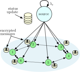
Figure 1: A gossip network consisting of a source and $n=6$ receiver nodes. Source encrypts status updates and sends them to nodes.

Motivated by these applications, we consider in this work an information source that generates updates and then encrypts them by using $(k,n)$-TSS. The source is able to send the encrypted messages to the $n$ receiver nodes instantaneously. Upon receiving these updates, the nodes start to share their local messages with their neighboring nodes to decrypt the source’s update. The nodes that get $k$ different messages of the same update from their neighbors can decode source’s information. We consider two different settings: a memory scheme where the nodes are able to keep the source’s current and previous encrypted messages and a memoryless scheme where the nodes are allowed to keep only the source’s current message. For both of these settings, we study the information freshness achieved by the receivers as a result of applying $(k,n)$-TSS.

In order to measure the freshness of information in communication networks, age of information (AoI) has been introduced as a new performance metric [8]. Since then, AoI has been considered in queueing networks [9], energy harvesting problems [10, 11], caching systems [12], remote estimation [13], distributed computation systems [14], and RF-powered communication systems [15]. A more detailed review of the literature on AoI can be found in [16]. The traditional age metric increases linearly over time until the receiver gets a new status update from the source. However, if the information at the source does not change frequently, although the receiver may not get updates from the source for a long time, the receiver may still have the most up-to-date information prevailing at the source. The traditional age metric is said to be source-agnostic, meaning that it does not consider the information change rate at the source. Considering this problem, new source-aware freshness metrics such as the version age of information [17, 18], the binary freshness [19], and age of incorrect information [20] have been considered recently which can achieve semantic-oriented communication [21].

In the earlier works on AoI, age has been studied for simple communication networks where the information flows through directly from the source, or other serially connected nodes (as in multi-hop multi-cast networks [22]). The development of the stochastic hybrid system (SHS) approach in [23] paves a new way to calculate the average age in arbitrarily connected networks. In particular, reference [17] considers a setting where in addition to source sending updates to the receiver nodes, nodes also share their local updates through a gossiping mechanism to improve their freshness further. Inspired by [17], reference [24] improves the AoI scaling by using the idea of clustered networks and [25] studies scaling of binary freshness metric in gossip networks. In the aforementioned works in [17, 24, 25], age scaling has been considered in disconnected, ring, and fully-connected symmetric gossip networks. Different from these symmetric gossip networks, age scaling has been studied in a grid network in [26]. Reference [27] optimizes age in a gossip network where updates are provided through an energy harvesting sensor. In gossiping, as the information exchanges happen through comparison of time-stamp of information, the gossip networks are vulnerable to adversarial attacks. The timestomping, i.e., changing time-stamp of the updates to brand the outdated information as fresh, has been studied in gossip networks in [28]. The reliability of information sources [29], the binary dynamic information dissemination [30], information mutation and spread of misinformation [31] have been studied in gossip networks. More recent advances of AoI in gossip networks can be found in [32].

In all these aforementioned works, the source sends its information to gossip nodes without using any encryption. For the first time, in this work, we consider the version age of information in a gossip network where the source encrypts the information via $(k,n)$-TSS. We study two different settings where ($i$) the nodes have memory, in which case they can hold the current and also the previous keys received from the source, and ($ii$) the nodes do not have memory, in which case they can only hold the keys from the most current update. For both schemes, we measure the freshness of the information through $k$-keys version age of information.

In this work, we first derive the relations necessary to obtain closed-form expressions for the time average of $k$-keys version age for an arbitrary non-homogeneous network (e.g., independently activated communication channels). Then, in the numerical results, we show that the time average of the $k$-keys version age for a node in both schemes decreases as the edge activation rate increases, or as the number of keys required to decode the information decreases, or as the number of gossip pairs in the network increases. We show that a memory scheme yields a lower time average of $k$-keys version age compared to a memoryless scheme. However, the difference between the two schemes diminishes with infrequent source updates, frequent gossip between nodes, or a decrease in $k$ for a fixed number of nodes $n$.

2 System Model and Metric

We consider an information updating system consisting of a single source, which is labeled as node $0$, and $n$ receiver nodes. The information at the source is updated at times distributed according to a Poisson counter, denoted by $N_{0}(t)$, with rate $\lambda_{s}$. We refer to the time interval between $\ell$th and $(\ell+1)$th information updates (messages) as the $\ell$th version cycle and denote it by $U^{\ell}$. Each update is stamped by the current value of the process $N_{0}(t)=\ell$ and the time of the $\ell$th update is labelled $\tau_{\ell}$ once it is generated. The stamp $\ell$ is called version-stamp of the information.

We assume that the source is able to instantaneously encrypt the information update by using $(k,n)$-TSS once it is generated. To be more precise, we assume that the source puts the information update into $n$ distinct keys and sends one of the unique keys to each receiver node at the time $\tau_{\ell}$, instantaneously. Once a node gets a unique key from the source at $\tau_{\ell}$ for version $\ell$, it is aware of that there is new information at the source. Each node wishes its knowledge of the source to be as timely as possible. The timeliness is measured for an arbitrary node $j$ by the difference between the latest version of the message at the source node, $N_{0}(t)$, and the latest version of the message which can be decrypted at node $j$, denoted by $N^{k}_{j}(t)$. This metric has been introduced as version age of information in [17, 18]. We call it $k$-keys version age of node $j$ at time $t$ and denote it as

$$A^{k}_{j}(t):=N_{0}(t)-N^{k}_{j}(t).\\$$ (1)

Recall that in the $(k,n)$-TSS, a node needs to have $k+1$ keys with the version stamp $\ell$ in order to decrypt the information at the source generated at $\tau_{\ell}$. Since the source sends a unique key to all receiver nodes, a node needs $k$ additional distinct keys with version $\ell$ to decrypt the $\ell$th message. We denote by $\vec{G}=(V,\vec{E})$ the directed graph with node set $V$ and edge set $\vec{E}$. We let $\vec{G}$ represent the communication network according to which nodes exchange information. If there is a directed edge $e_{ij}\in\vec{E}$, we call node $j$ gossiping neighbor of node $i$. We call a communication network $(k,n)$-TSS feasible if the node $0$ has out-bound connections to all other nodes and the smallest in-degree of the receiver nodes is greater than $k$. We illustrate in Fig. 1 a $(2,6)$-TSS feasible network.

In this work, we consider a $(k,n)$-TSS feasible network, in which, nodes are allowed to communicate and share only the keys that are received from the source with their gossiping neighbor. The edge $e_{ij}$, which connects node $i$ to node $j$, is activated at times distributed according to the Poisson counter $N^{ij}(t)$, which has a rate $\lambda_{ij}$. All counters are pairwise independent. Once the edge $e_{ij}$ is activated, node $i$ sends a message to node $j$, instantaneously. This process occurs under two distinct schemes: with memory scheme and memoryless scheme.

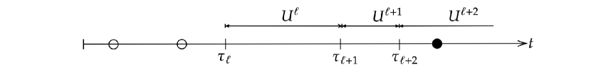
Figure 2: Sample timeline of the source update and the edge $e_{ij}$ activation. The last activation of $e_{ij}$ is marked by ($\bullet)$ and the previous activations of $e_{ij}$ are marked by ($\circ$).

In the memory scheme, nodes can store (and send) the keys of the previous updates. For example, if the edge $e_{ij}$ is activated at $t$, node $i$ sends node $j$ all the keys that the source has sent to node $i$ since the last activation of $N^{ij}(t)$ before $t$. For the illustration in Fig. 2, node $i$ sends the set of keys with the versions $\{\ell,\ell+1,\ell+2\}$ to node $j$ in the memory scheme. Note that this can be implemented by finite memory in a finite node network with probability $1$; we will provide below the distribution of the number of keys in the message. In the memoryless scheme, nodes have no memory and only store the latest key obtained from the source. If the edge $e_{ij}$ is activated at $t$, node $i$ sends node $j$ only the last key that the source sent to node $i$ before $t$. Referring again to the illustration in Fig. 2, node $i$ in this case sends only the key with the version $\{\ell+2\}$ to node $j$.

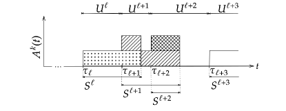
(a)

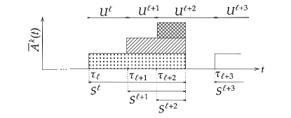
(b)

Figure 3: Sample path of the $k$-keys version age (a) $A^{k}(t)$ for a node with memory and (b) $\bar{A}^{k}(t)$ for a node without memory.

Fig. 3(a) and Fig. 3(b) depict the sample path of the $k$-keys version age process ${A}^{k}(t)$ (resp.  $\bar{A}^{k}(t)$) for a node with memory (resp. without memory). It is worth noting that we associate the notation $\bar{\cdot}$ with the memoryless scheme. It is assumed that edge activations and source updates occur at the same time in both schemes in the figures. In the memory scheme, we define the service time of information with version $\ell$ to an arbitrary node $j$, denoted by $S^{\ell}_{j}$, as the duration between $\tau_{\ell}$ and the time when node $j$ can decrypt the information with version $\ell$, as shown in Fig. 3(a). In the memoryless scheme, a node can miss an information update with version $\ell$, in contrast to the memory scheme, if it cannot get $k$ more distinct keys before the next update arrives at $\tau_{\ell+1}$. Thus, for a node without memory, we define $S^{\ell}_{j}$ as the duration between $\tau_{\ell}$ and the time when the node can decrypt information with a version greater than or equal to $\ell$. In Fig. 3(b), the node misses the information with versions $\ell$ and $\ell\!+\!1$. It can only decode the information with version $\ell\!+\!2$. Therefore, the service times $S^{\ell}$ and $S^{\ell+1}$ end at the same time as the service time $S^{\ell+2}$ ends.

Let $\Delta^{k}_{j}(t)$ be the total $k$-keys version age of node $j$, defined as the integrated $k$-keys version age of node $j$, $A^{k}_{j}(\tau)$, until time $t$. For both schemes, the time average of $k$-keys version age process of node $j$ is defined as follows:

$$\Delta^{k}_{j}:=\lim_{t\to\infty}\frac{\Delta^{k}_{j}(t)}{t}=\lim_{t\to\infty}\frac{1}{t}\int_{0}^{t}A^{k}_{j}(\tau)d\tau.$$ (2)

We interchangeably call $\Delta^{k}_{j}$ the version age of $k$-keys TSS for node $j$. If nodes in the network have no memory, we denote the version age of $k$-keys TSS for node $j$ by $\bar{\Delta}^{k}_{j}$.

3 Age Analysis

In this section, we first introduce the main concepts that will be useful for deriving age expressions and then provide closed-form expressions for the version age of $k$-keys TSS scheme with and without using the memory, which are the main results of the paper.

We first focus on the order statistic of a set of random variables. Consider a set of random variables $\mathcal{Y}=\{Y_{i}\}_{i=1}^{n}$. We denote the $k^{th}$ smallest variable in the set $\mathcal{Y}$ by $Y_{(k:n)}$. We call $Y_{(k:n)}$ the $k$th order statistic of $n$-samples ($k=1,2,\cdots,n$) in the set $\mathcal{Y}$. For a set of $i.i.d$ random variables $\{Y_{i}\}_{i=1}^{n}$ from an exponential distribution with mean $\frac{1}{\lambda}$, the expectation of the $k$th order statistic $Y_{(k:n)}$ is given by [33]:

$$\mathbb{E}[Y_{(k:n)}]=\frac{1}{\lambda}(H_{n}-H_{n-k}),\mbox{ where }H_{n}=\sum_{j=1}^{n}\frac{1}{j}.\\$$ (3)

Let $\mathcal{N}^{+}_{j}=\{i\in V,e_{ij}\in\vec{E}\}$ be the set of nodes with out-bound connections to node $j$; denote its cardinality by $n_{j}$. Let $X_{ij}$ be the times between successive activations of the edge $e_{ij}$. Then, $X_{ij}$ is an exponential random variable with mean $1/\lambda_{ij}$. Let $\mathcal{X}_{j}$ be the set of random variables $X_{ij}$, $\forall i\in\mathcal{N}^{+}_{j}$. Let $\mathcal{I}^{j}$ be a set of indices that label the elements of the set $\mathcal{X}_{j}$. With this notation, we can express the cumulative density function (c.d.f.) of the $k$th order statistic of the set $\mathcal{X}_{j}$ as follows:

$$\!F_{k}(x,\mathcal{X}_{j})\!=\!\sum^{n_{j}}_{i=k}\sum_{{S_{i}}}\left(\prod_{\ell=1}^{i}F_{m_{\ell}}(x)\prod_{\ell=i+1}^{n_{j}}(1-F_{m_{\ell}}(x))\right),\!\!$$ (4)

where the summation $S_{i}$ extends over all permutations $(m_{1},m_{2},\cdots,m_{n_{j}})$ of the set $\mathcal{I}^{j}$ [33]. We denote the $k$th order statistic of the set $\mathcal{X}_{j}$ by $\mathcal{X}_{(k:n_{j})}$.

3.1 Nodes with Memory

In this subsection, we first compute the service time of the information to a node with memory. Then, we provide the closed-form expression for the version age of $k$-keys TSS, ${\Delta}^{k}_{j}$, for any node in a $(k,n)$-TSS feasible network.

Lemma 1.

If nodes have memory, then the service time of the information with version $\ell$ to node $j$ is the $k$th order statistic of the set of exponential random variables $\mathcal{X}_{j}$.

Proof.

We denote the set of the first activation times of edges that are connected to the node after $\tau_{\ell}$ by $\mathcal{X}^{\ell}$. For the case $\mathcal{X}^{\ell}_{(k:n_{j})}\leq U^{\ell}$, the result trivially follows from the definitions. Consider the case $\mathcal{X}^{\ell}_{(k:n_{j})}>U^{\ell}$. By definition, a new status update arrives at all nodes at $\tau_{\ell+1}(=\tau_{\ell}+U^{\ell}$). However, the structure of a message sent after $\tau_{\ell+1}$ from a node to another node ensures that it has the key with version stamp $\ell$. Therefore, the service time for a status update is also $\mathcal{X}^{\ell}_{(k:n_{j})}$ (regardless of the fact that a new update arrived). ∎

We are now in a position to state the main theorem.

Theorem 1.

Let $\vec{G}$ be a $(k,n)$-TSS feasible network. Consider an arbitrary node $j$ in $\vec{G}$. The version age of $k$-keys TSS for node $j$ with memory is:

$$\Delta^{k}_{j}=\frac{\mathbb{E}[\mathcal{X}_{(k:{n}_{j})}]}{\mathbb{E}[U]}\mbox{ w.p. }1.$$ (5)

where $U$ is the interarrival time for the source update.

See Appendix 6.2 for the complete proof of Theorem 1. We outline here the basic steps involved. Let $T:=\{\tau_{l}\}_{l=0}^{\infty}$ be the monotonically increasing sequence of times when the status updates occur at the source node $0$, with $\tau_{0}\!:=\!0$. Let $T^{1}\!=\!\{\tau_{\ell_{a}}\}_{a=0}^{\infty}$ be a subsequence of $T$ such that $A^{k}(\tau_{\ell_{a}})\!=\!1$. In words, the subsequence $T^{1}$ is the sequence of information update times which the node can decrypt the current status update beforehand. For example, recalling Fig. 3(a), the node can decrypt the current status update before a new one arrives at $\tau_{\ell}$ and $\tau_{\ell+3}$. Therefore, the information update times $\tau_{\ell}$ and $\tau_{\ell+3}$ are in $T^{1}$ for the given sample path. Let $R^{a}$ be the integrated $k$-keys version age of a node between times $\tau_{\ell_{a}}$ and $\tau_{\ell_{a+1}}$. One can easily see that a pair of $(R^{a},R^{b})$ for any $a\neq b$ is $i.i.d.$ As a corollary of Lemma 1, recalling Fig. 3(a), the sum of service times between two consecutive elements of $T^{1}$ corresponds to the sum of three different shaded areas, that is, $R^{a}\!=S^{\ell}\!+\!S^{\ell+1}\!+\!S^{\ell+2}$ and the elapsed time between two consecutive elements of $T^{1}$ is equal to $U^{\ell}\!+\!U^{\ell+1}\!+\!U^{\ell+2}$. From the Reward Renewal Theorem (see Appendix 6.1), the result follows. One can easily obtain an explicit form of $\Delta^{k}$ by using the c.d.f. in (4).

The case of a fully connected directed graph $\vec{G}$ on $n+1$ nodes (including the source node) with $\lambda_{ij}=\frac{\lambda_{e}}{(n-1)}$ for all edges $e_{ij}$ in $\vec{E}$, is called scalable homogeneous network and $\lambda_{e}$ is the gossip rate. In a scalable homogeneous network, the processes $A^{k}_{j}(t)$ are statistically identical for any node $j$. Thus, we denote the set $\mathcal{X}_{j}$ by $\mathcal{X}$ for any node $j\in V$.

Corollary 1.1.

For a scalable homogeneous network, the version age of $k$-keys TSS for a node with memory is:

$$\Delta^{k}=\frac{\mathbb{E}[\mathcal{X}_{(k:n-1)}]}{\mathbb{E}[U]}=\frac{(n-1)\lambda_{s}}{\lambda_{e}}(H_{n-1}-H_{n-1-k})\mbox{ w.p. }1.$$

Corollary 1.2.

For a finite $k$ and a scalable homogeneous network with a countable memory, we have the following scalability result:

$$\lim_{n\to\infty}\Delta^{k}=\frac{k\lambda_{s}}{\lambda_{e}}\mbox{ w.p. }1.$$

We now elaborate on the number of keys in the message that is sent over an edge. To this end, let $\mathcal{M}^{i}_{j}$ be the number of keys in the message that is sent over the edge $e_{ij}$. In each update cycle, either the source’s update takes place before the edge’s activation in which case $\mathcal{M}^{i}_{j}$ increases by 1 or the edge is activated before a source update in which case node $i$ sends all the keys to node $j$, and thus $\mathcal{M}^{i}_{j}$ reduces to 0. Due to [34, Prob. 9.4.1], $\mathcal{M}^{i}_{j}$ has a geometric distribution with success probability $\frac{\lambda_{e_{ij}}}{\lambda_{e_{ij}}+\lambda_{s}}$. It shows that the expected number of keys in the message between nodes rises as the source rate update $\lambda_{s}$ increases or the edge activation rate $\lambda_{e_{ij}}$ decreases. In the following subsection, we analyze the memoryless scheme.

3.2 Nodes without Memory

In this subsection, we provide a closed-form expression for the version age of $k$-keys TSS for any node without memory, $\bar{\Delta}^{k}_{j}$, in a $(k,n)$-TSS feasible network.

Theorem 2.

Let $\vec{G}$ be a $(k,n)$-TSS feasible network. The version age of $k$-keys TSS for node $j$ without memory is:

$$\bar{\Delta}^{k}_{j}=\frac{\mathbb{E}[\min(\mathcal{X}_{(k:{n}_{j})},U)]}{Pr(\mathcal{X}_{(k:{n_{j}})}\!\leq\!U)\mathbb{E}[U]}\mbox{ w.p. }1$$ (6)

where $U$ is the interarrival times for the source update.

See Appendix 6.3 for a proof of Theorem 2. One can easily compute $\bar{\Delta}^{k}_{j}$ and $Pr(\mathcal{X}_{(k:{n_{j}})}\!\leq\!U)$ by using (4). We can focus on the statement of Theorem 2. In the memoryless scheme, a node needs to get at least $k$ different keys with version $\ell$ before $\tau_{\ell+1}$ so that it can decrypt the status update generated at $\tau_{\ell}$. To be more precise, a node can decode the status update at $\tau_{\ell}$ if the event $E=\{\mathcal{X}_{(k:n_{j})}\!\leq\!U^{\ell}\}$ happens, otherwise, it misses. Then, Theorem 2 says that if the event $E$ happens in an update cycle, the accumulated age in the update cycle is $\mathcal{X}_{(k:n_{j})}$, otherwise, it is $U^{\ell}$. The expected time of the generation of two consecutive status updates that can be decrypted at node $j$ is equal to $Pr(E)\mathbb{E}[U]$ (see Appendix 6.3 Lemma 2).

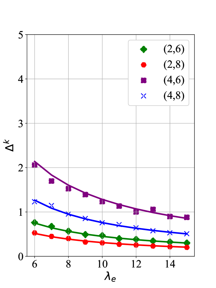
(a)

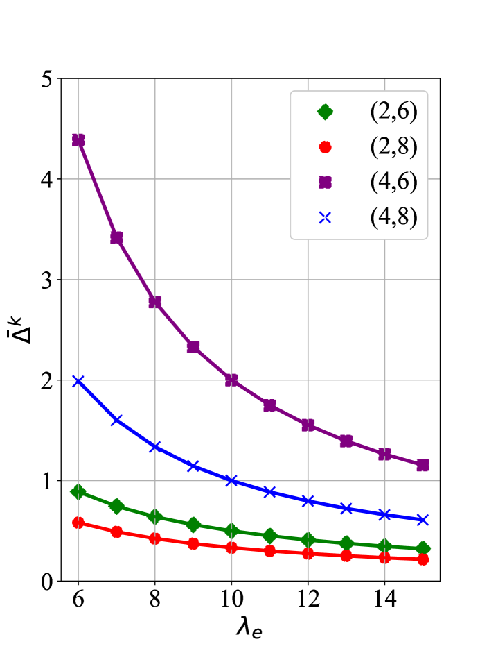
(b)

Figure 4: (a) $\Delta^{k}$ and (b) $\bar{\Delta}^{k}$ as a function of $\lambda_{e}$ on a scalable homogeneous network when $\lambda_{s}=10$. Solid lines in Fig. 4(a) show theoretical $\Delta^{k}$ while solid lines in Fig. 4(b) show theoretical $\bar{\Delta}^{k}$. Simulation results for $(2,6)$,$(2,8)$,$(4,6)$,$(4,8)$ TSS are marked by $\blacklozenge,\bullet,\blacksquare,\times$, respectively.

Corollary 2.1.

For a scalable homogeneous network, the version age of $k$-keys TSS for an individual node without memory is:

$$\bar{\Delta}^{k}=\frac{\frac{\lambda_{s}}{\lambda_{e}\!+\!\lambda_{s}}\!+\!\sum\limits_{j=2}^{k}\left(\frac{\lambda_{s}}{\lambda_{e}\mathcal{B}(n,j)\!+\!\lambda_{s}}\!\prod\limits_{i=1}^{j\!-\!1}\frac{\lambda_{e}\mathcal{B}(n,i)}{\lambda_{e}\mathcal{B}(n,i)\!+\!\lambda_{s}}\right)}{Pr(E)}\mbox{ w.p. }1$$ (7)

where the event $E$ is $\{\mathcal{X}_{(k:n-1)}\leq U\}$ and $\mathcal{B}(n,i)=\frac{(n-i)}{(n-1)}$.

See Appendix 6.4 for a proof of Corollary 2.1.

4 Numerical Results

In this section, we provide numerical results for the version age of $(k,n)$-TSS with and without memory schemes. In particular, we compare empirical results obtained from simulations to our analytical results.

In the first set of results, we consider a scalable homogeneous network. Fig. 4 depicts the simulation and the theoretical results for both $\Delta^{k}$ and $\bar{\Delta}^{k}$ as a function of gossip rate $\lambda_{e}$ when $\lambda_{s}=10$. The simulation results for $\Delta^{k}$ and $\bar{\Delta}^{k}$ align closely with the theoretical calculations provided in Thm.1 and Thm. 2, respectively. In both schemes, we observe that the version age of $k$-keys TSS for a node increases with the rise in the gossip rate $\lambda_{e}$, while keeping the network size $n$ and $\lambda_{s}$ constant. Fig. 4(a) also depicts the version age of $k$-keys TSS as a function of the pair $(k,n)$. We observe, in Fig. 4(a), that $\Delta^{k}$ increases with the growth of $k$ for a fixed $\lambda_{e}$ and $n$ and it decreases as $n$ increases for fixed $\lambda_{e}$ and $k$. On the one hand, Fig. 4(b) confirms that the earlier observation regarding $\Delta^{k}$ and its connection with network parameters $\lambda_{e}$ and $(k,n)$ also holds true for $\bar{\Delta}^{k}$. On the other hand, we observe, in Fig. 4, that the version age of $k$-keys TSS in the with memory scheme $\Delta^{k}$ is less than the version age of $k$-keys TSS in the without memory scheme $\bar{\Delta}^{k}$ for the same values of $\lambda_{e},\lambda_{s}$ and $(k,n)$.

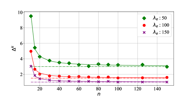
Figure 5: $\Delta^{k}$ as a function of $n$ when $k=10$ and $\lambda_{s}=15$. Solid lines show the theoretical $\Delta^{k}$ while simulation results for $\lambda_{e}=\{50,100,150\}$ selections are marked by $\blacklozenge,\bullet,\times$, respectively. Dashed lines show the theoretical asymptotic value of $\Delta^{k}$ on $n$.

Fig. 5 depicts $\Delta^{k}$ as a function of the number of the nodes $n$ for various gossip rates $\lambda_{e}$. We observe, in Fig. 5, that $\Delta^{k}$ converges to $\frac{k\lambda_{s}}{\lambda_{e}}$ as $n$ grows. It aligns with Cor. 1.2.

5 Discussion on The Value of Memory

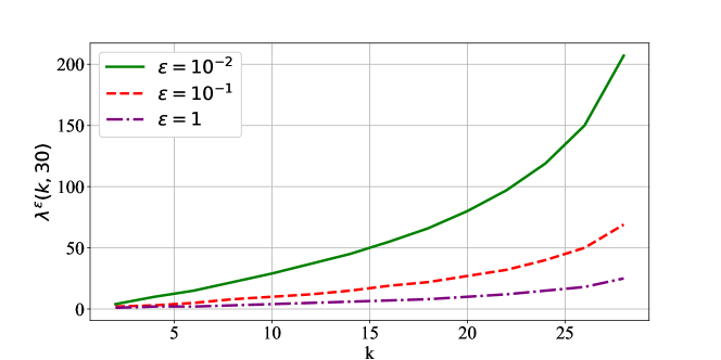
Figure 6: The smallest gossip rate $\lambda_{e}$ such that $|\Delta^{k}-\bar{\Delta}^{k}|\leq\varepsilon$ as a function of $k$ for fixed $n=30$ and $\lambda_{s}=15$. Solid line, dashed line and dotted-dashed line show $\lambda^{\varepsilon}$ for $\varepsilon=10^{-2},\varepsilon=10^{-1}$ and $\varepsilon=1$, respectively.

To quantify the value of memory in a network, we define the memory critical gossip rate of a $(k,n)$-TSS network for a margin $\varepsilon$, denoted by $\lambda^{\varepsilon}(k,n)$, as the smallest gossip rate $\lambda_{e}$ such that $|\Delta^{k}-\bar{\Delta}^{k}|\leq\varepsilon$. Fig. 6 depicts the memory critical gossip rate of a $(k,30)$-TSS network for different margins as a function of $k$. We first observe, in Fig. 6, that the memory critical gossip rate $\lambda^{\varepsilon}(k,n)$ increases as the margin $\varepsilon$ decreases, and it exponentially increases as $k$ increases for fixed $n$. These observations show that $\bar{\Delta}^{k}$ approaches ${\Delta}^{k}$ as $\lambda_{e}$ increases or $k$ decreases. These results align with Cor. 1.1. Consider the event $E\!:=\!\{\mathcal{X}_{(k:n-1)}\leq U\}$ (event that a node can decrypt the status update before a new status update arrives); one can easily see that the probability of event $E$ converges to $1$ as the gossip rate $\lambda_{e}$ increases or $k$ decreases for fixed $n$. It implies that the service time of any status update approaches the random variable $\mathcal{X}_{(k:n-1)}$ as $Pr(E)$ goes to $1$. In this case, by construction, the expectation $\mathbb{E}[\mathds{1}_{\{E^{c}\}}U]\!\to\!0$ and the expectation $\mathbb{E}[\mathds{1}_{\{E\}}\mathcal{X}_{(k:n-1)}]\!\to\!\mathbb{E}[\mathcal{X}_{(k:n-1)}]$ in (6). It implies that the version age of $k$-keys TSS for a node without memory $\bar{\Delta}^{k}$ approach to the version age of $k$-keys TSS for a node with memory $\Delta^{k}$ as $Pr(E)$ goes to $1$.

6 Conclusion

We have examined an information update system consisting of $n$-receiver nodes and a single source that encrypts the information by using $(k,n)$-TSS. We have provided closed-form expressions for the version age of $k$-keys TSS for both with memory and memoryless schemes. The evaluations have shown that the version age of $k$-keys TSS for a node with memory $\Delta^{k}$ is less than the version age of $k$-keys TSS for a node without memory $\bar{\Delta}^{k}$ on the same network. We have observed that if gossip occurs fast enough or the source is updated slowly enough, the memoryless scheme results in the same version age of $k$-keys TSS as the memory scheme does. For a scalable homogeneous network, in which the gossip rate is uniform, we have shown that $\Delta^{k}$ converges to $k\lambda_{s}/\lambda_{e}$ as the network grows. In our work, nodes only send the keys that are received from the source node, ensuring that any set of messages on the channels is not sufficient to decrypt the message at any time. An alternative approach might be to consider the case where nodes can share keys that are received from other nodes. For such a scheme, in future work, we aim to compute the version age of $k$-keys TSS as a function of the number of keys in a message and find the optimal message structure. Another future research direction would be to compute the version age of $k$-keys TSS when there are informative keys in the network.

APPENDICES

6.1 Reward Renewal Process

Let $Z=((S_{0},R_{0}),(S_{1},R_{1}),\cdots)$ be sequence of interarrival times and rewards. Suppose that the rewards are nonnegative and that $A=\left\{A_{t}:t\in[0,\infty)\right\}$ is a nonnegative stochastic process with:

1. $t\mapsto Y_{t}$ piecewise continuous.

2. $R_{n+1}=\int_{T_{n}}^{T_{n+1}}A_{t}dt$ for $n\in\mathbb{N}$

where $\{T_{n}\}$ is corresponding the sequence of time of arrivals, that is, $T_{n}:=\sum_{i=0}^{n}S_{i}$. Let $\Delta_{t}=\int_{0}^{t}A_{s}ds$ for $t\in[0,\infty)$. If the interarrival times and reward pairs, $Z=(S_{0},R_{0}),(S_{1},R_{1}),\cdots)$ form an independent and identically distributed sequence of random variables, then $\Delta=\left\{\Delta_{t}:t\in[0,\infty)\right\}$ is a reward process associated with $Z$.

For a reward process associated with a sequence of interarrival times and rewards, we have the following Theorem.

Theorem 3 (Reward Renewal Theorem,[35]).

Suppose that $\Delta_{t}$ for $t\in[0,\infty)$ is reward process associated with $Z=((S_{0},R_{0}),(S_{1},R_{1}),\cdots)$. Let $\delta(t)=\mathbb{E}[\Delta_{t}]$ for $t\in[0,\infty)$ . Then, we have:

1. $\frac{\Delta_{t}}{t}\to\frac{\mathbb{E}[R]}{\mathbb{E}[S]}$ as $t\to\infty$ with probability $1$.

2. $\frac{\delta_{t}}{t}\to\frac{\mathbb{E}[R]}{\mathbb{E}[S]}$ as $t\to\infty$.

where $\mathbb{E}[R]=\mathbb{E}[R_{n}]$ and $\mathbb{E}[S]=\mathbb{E}[S_{n}]$.

6.2 Proof of Thorem 1

Proof of Theorem 1.

Recall the definition of the subsequence $T^{1}$. We define $T^{1}=\{\tau_{\ell_{a}}\}_{a=0}^{\infty}$ as a subsequence of $T$ such that $A^{k}(\tau_{\ell_{a}})=1$. Let $L^{a}$ be the elapsed time between two consecutive successful arrivals of the subsequence $T^{1}$. If $A[\ell]=1$, it means that the node could decrypt the information version $\ell-1$ before $\tau_{\ell}$. We know that it is the event $E^{\ell}=\{X^{\ell-1}_{k:n-1}<U^{\ell-1}\}$. One can easily see that two events $E^{\ell}$ and $E^{\ell+1}$ are independent. It results in that the elapsed time between two successful arrivals of subsequence $T^{1}$ is independent $L=(L^{0},L^{1},\cdots)$ is a sequence of $i.i.d$ random variables. Let $R^{a}$ be version age of $k$-keys integrated over the duration $[\tau_{l_{a}},\tau_{l_{a+1}})$ in a node, that is,

$$R^{a}=\int_{\tau_{l_{a}}}^{\tau_{l_{a+1}}}A^{k}(s)ds$$

By construction, a pair of $(R^{a},R^{b})$ for any $a\neq b$ is $i.i.d.$. This implies that $R=(R^{0},R^{1},\cdots)$ is a sequence of $i.i.d.$ random variables. From the definition of reward renewal process in Appendix 6.1, $\Delta(t)$ is reward renewal process associated with $Z=((L^{0},R^{0}),(L^{1},R^{1}),\cdots)$. From Theorem 3, we have the following limit:

$$\lim_{t\to\infty}\frac{\Delta(t)}{t}=\frac{\mathbb{E}[R^{a}]}{\mathbb{E}[L^{a}]}\mbox{ w.p. }1.$$

By definition, the random variable $R^{a}$ is the sum of service times of the source updates with version $i$ to the node for $\ell_{a}\leq i\leq\ell_{a+1}-1$. From Lemma 1, we have:

$$\frac{\mathbb{E}[R^{a}]}{\mathbb{E}[L^{a}]} =\frac{\mathbb{E}[\sum_{i=\ell_{a}}^{\ell_{a+1}-1}S^{i}_{j}]}{\mathbb{E}[\sum_{i=\ell_{a}}^{\ell_{a+1}-1}U^{i}]}=\frac{\mathbb{E}[\sum_{i=\ell_{a}}^{\ell_{a+1}-1}\mathcal{X}^{i}_{(k:n_{j})}]}{\mathbb{E}[\sum_{i=\ell_{a}}^{\ell_{a+1}-1}U^{i}]}$$

$$=\frac{\sum_{i=l_{a}}^{l_{a+1}-1}\mathbb{E}[\mathcal{X}^{i}_{(k:n_{j})}]}{\sum_{i=\ell_{a}}^{\ell_{a+1}-1}\mathbb{E}[U^{i}]}=\frac{\mathbb{E}[X_{k:n_{j}}]}{{E}\mathbb{[}U]}$$

where $\mathbb{E}[\mathcal{X}_{(k:n_{j})}]=\mathbb{E}[\mathcal{X}^{i}_{(k:n_{j})}]$ and $\mathbb{E}[U]=\mathbb{E}[U^{i}]$ for any $i$. It is worth noting that two random variables $\mathcal{X}^{i}_{(k:n_{j})}$ and $\mathcal{X}^{i+1}_{(k:n_{j})}$ are not independent in the memory scheme if $\ell_{a}\!\leq\!i\!\leq\!\ell_{a+1}-1$ for any $a\in\mathbb{N}$, but they are identically distributed. This completes the proof. ∎

6.3 Proof of Theorem 2

Consider $(k,n)$-TSS on nodes without memory. In this scheme, a node needs to get at least $k$ different keys with version stamp $\ell$ before $\tau_{\ell+1}$ so that it can decrypt the status update generated at $\tau_{\ell}$. To be more precise, a node can decode the status update $\ell$ if $\mathcal{X}^{j}_{(k:n_{j})}\leq U$ holds, otherwise, it misses.

Lemma 2.

Let $A_{j}[\ell]$ be the version age of information at $\tau_{\ell}$ for the node $j$. In a memoryless scheme, the sequence $A_{j}[\ell]$ is homogeneous success-run with the rate $\mu_{j}=Pr(\mathcal{X}^{j}_{(k:n_{j})}\leq U)$.

Proof.

We remove the index $j$ on notation, as it would be sufficient to prove the results for an arbitrary node. By abuse of notation, we denote the set of the first arrival times of edges that are connected to the node after $\tau_{\ell}$ by $\mathcal{X}^{\ell}$. One can easily show that $(\mathcal{X}^{\ell}_{(k:n-1)},U^{\ell})$ and $(\mathcal{X}^{\ell+1}_{(k:n-1)},U^{\ell+1})$ for any $\ell$ are independent. This implies that $A[\ell]$ has Markov property and it evolves as follows:

$$A[\ell+1]=\begin{cases}1&\mbox{if }\mathcal{X}^{\ell}_{(k:n-1)}\leq U^{\ell}\\ A[\ell]+1&\mbox{if }\mathcal{X}^{\ell}_{(k:n-1)}>U^{\ell}\end{cases}$$ (8)

and $A[0]$ is $1$ by definition. It follows that $A[\ell]$ is a discrete-time Markov chain on infinite states $\mathcal{A}:=\{1,2,\cdots\}$ with the initial distribution $\pi=[1,0,0,\cdots]$ and the state transition matrix of $P$

$$P:=\left[\begin{smallmatrix}\mu&1-\mu&&&\cdots\\ \mu&&1-\mu&&\cdots\\ \mu&&&1-\mu&\cdots\\ \vdots&&&&\ddots&\end{smallmatrix}\right]$$

where $\mu=Pr(\mathcal{X}^{\ell}_{(k:n-1)}\leq U^{\ell})$. This then says that the sequence $A[\ell]$ is a homogeneous success-run chain with rate $\mu$. ∎

As an easy corollary to Lemma 2, the random variable $A_{j}[\ell]$ has truncated geometric distribution at $\ell+1$ with success rate $\mu_{j}$. As $\ell$ goes to infinity, $\mathbb{E}[A_{j}[\ell]]$ goes to $1/\mu_{j}$ for node $j$.

Now, we can prove Theorem 2.

Proof of Theorem 2.

By abuse of notation, we remove the index $j$ on notation as it is sufficient to prove the result for an arbitrary node. We have the stochastic process $\bar{A}^{k}(t)$ defined in (1). Recall the condition for the reward process provided in Appendix 6.1. Then, one can compute $R_{\ell}$ (defined in Appendix 6.1) as follows:

$$R_{\ell} =\int_{\tau_{\ell-1}}^{\tau_{\ell}}\bar{A}^{k}(t)dt$$ (9)

$$R_{\ell} =A[\ell-1](\mathds{1}_{E}\mathcal{X}^{\ell-1}_{(k:n-1)}+\mathds{1}_{E^{c}}U^{\ell-1})$$ (10)

where the event $E=\{\mathcal{X}^{\ell-1}_{(k:n-1)}\leq U^{\ell-1}\}$ and we denote complement by $E^{c}$. Then, this says that the process $\bar{\Delta}^{k}(t)$ is a reward process associated with $Z=((U_{1},R_{1}),(U_{2},R_{2}),\cdots)$. Let $E[A]$ be the expectation of $A[\ell]$ where $\ell$ goes to infinity. From Theorem 3 and (9), we can compute the expectation of $R_{\ell}$ as $\ell$ goes to infinity, denoted by $\mathbb{E}[R]$, as follows:

$$\mathbb{E}[R]=\mathbb{E}[A](\mathbb{E}[\mathds{1}_{E}\mathcal{X}_{(k:n-1)}]+\mathbb{E}[\mathds{1}_{E^{c}}U])$$

It is worth noting that the event $E$ and the pair of random variables $(\mathcal{X}_{(k:n-1)},U)$ are not independent. As a corollary of Theorem 3, we have the following:

$$\frac{\Delta^{k}(t)}{t}\to\frac{\mathbb{E}[A](\mathbb{E}[\mathds{1}_{E}\mathcal{X}_{(k:n-1)}]+\mathbb{E}[\mathds{1}_{E^{c}}U])}{\mathbb{E}[U]}\mbox{ w.p. }1\mbox{ as }t\to\infty.$$

From Lemma 2, we know that $\mathbb{E}[A]=\frac{1}{\mu}$ where $\mu=Pr(E)$. Then, we have the following.

$$\Delta^{k}=\lim_{t\to\infty}\frac{\Delta^{k}(t)}{t} =\frac{\mathbb{E}[\mathds{1}_{E}\mathcal{X}_{(k:n-1)}]+\mathbb{E}[\mathds{1}_{E^{c}}U]}{Pr(E)\mathbb{E}[U]}\mbox{ w.p. }1$$

$$=\frac{\mathbb{E}[\min(\mathcal{X}_{(k:n-1)},U)]}{Pr(E)\mathbb{E}[U]}\mbox{ w.p. }1$$

It completes the proof. ∎

6.4 Proof of Corollary 2.1

Consider an individual node in a scalable homogeneous network and let us focus on an arbitrary update cycle $\ell$. Recall the set $\mathcal{X}$, it is the set of the elapsed time between the first activation of edges connected to the node and $\tau_{\ell}$. In a scalable homogenous network, the set $\mathcal{X}$ is a set of $i.i.d.$ random variables from an exponential distribution with mean $\frac{(n-1)}{\lambda_{e}}$.

Let $Y^{k}$ be $\min\{\mathcal{X}_{(k:n-1)},U\}$. We need to find $\mathbb{E}[Y^{k}]$ to compute (6). Let $\tilde{X}_{i:n-1}$ be the difference between $i$th and $(i\!-\!1)$th order statistics of the set $\mathcal{X}$ for $i>0$ and $\tilde{X}_{1:n-1}\!=\!\mathcal{X}_{(1:n-1)}$. Thus, by construction, we have:

$$\mathcal{X}_{(k:n-1)}=\sum_{j=1}^{k}\tilde{X}_{j:n-1}$$

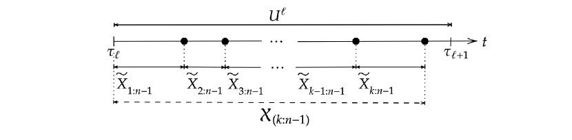
Figure 7: Sample timeline of the source update and the activation of edges that are all connected to a unique node. The time of activation of each edge is marked by ​($\bullet).$

Let $\tilde{Y}_{i}=\min\{\tilde{X}_{i:n-1},U^{\ell}\}$. One can see that, from memoryless property, the random variable $\tilde{X}_{i:n-1}$ corresponds to the minimum of a set of $(n\!-\!i)$ $i.i.d.$ random variables from an exponential distribution with mean $\frac{(n-1)}{\lambda_{e}}$. Thus, the random variable $\tilde{X}_{i:n-1}$ is also an exponential random variable, the parameter of which is equal to the sum of the parameters of $(n-i)$ $i.i.d.$ random variables, and precisely its mean is equal to $\frac{(n-1)}{\lambda_{e}(n-i)}$. This implies that the random variable $\tilde{Y}_{i}$ is the minimum of two independent exponentially distributed random variables. From [34, Prob. 9.4.1], the random variable $\tilde{Y}_{i}$ is exponentially distributed with the mean

$$\mathbb{E}[\tilde{Y}_{i}]=\frac{1}{\lambda_{e}\frac{(n-i)}{(n-1)}+\lambda_{s}},$$ (11)

and $Pr(U^{\ell}\!>\!\tilde{X}_{i:n-1})$ for some $0<i<n$, can be found as:

$$Pr(U^{\ell}\!>\!\tilde{X}_{i:n-1})=\frac{\lambda_{e}\!\frac{(n-i)}{(n-1)}}{\lambda_{e}\!\frac{(n-i)}{(n-1)}\!+\!\lambda_{s}}.$$ (12)

From the total law of expectation and memoryless property of $U^{\ell}$, we have the following:

$$\mathbb{E}[Y^{k}]= Pr(U^{\ell}\!\leq\!\tilde{X}_{1:n-1})\mathbb{E}[\tilde{Y}_{1}]$$

$$+\!\!Pr(U^{\ell}\!\leq\!\tilde{X}_{2:n-1})Pr(\!U^{\ell}\!\!>\!\!\tilde{X}_{1:n-1}\!)(\mathbb{E}[\tilde{Y}_{1}]\!\!+\!\!\mathbb{E}[\tilde{Y}_{2}])$$

$$\vdots$$

$$+\!\!Pr(U^{\ell}\!\leq\!\tilde{X}_{i:n-1})\!\prod_{i=1}^{k-2}Pr(U^{\ell}\!>\!\tilde{X}_{i:n-1})\!\sum_{i=1}^{k-1}\!\mathbb{E}[\tilde{Y}_{i}]$$

$$+\prod_{i=1}^{k-1}Pr(U^{\ell}\!>\!\tilde{X}_{i:n-1})(\sum_{i=1}^{k-1}\mathbb{E}[\tilde{Y}_{i}])$$

If we rearrange the sum above, we obtain:

$$\mathbb{E}[Y^{k}]=\mathbb{E}[\tilde{Y}_{1}]+\sum_{j=2}^{k}\left(\mathbb{E}[\tilde{Y}_{j}]\prod_{i=1}^{j-1}Pr(U^{\ell}\!>\!\tilde{X}_{i:n-1})\right).\!$$ (13)

If we plug $\mathbb{E}[\tilde{Y}_{i}]$ in (11) and $Pr(U^{\ell}\!>\!\tilde{X}_{i:n-1})$ in (12) for $i\geq 1$ into (13), we have:

$$\mathbb{E}[Y^{k}]\!=\!\frac{1}{\lambda_{e}\!+\!\lambda_{s}}\!+\!\!\sum_{j=2}^{k}\!\left(\!\frac{1}{\lambda_{e}\!\frac{(n-j)}{(n-1)}\!+\!\lambda_{s}}\!\prod_{i=1}^{j-1}\frac{\lambda_{e}\!\frac{(n-i)}{(n-1)}}{\lambda_{e}\!\frac{(n-i)}{(n-1)}\!+\!\lambda_{s}}\right)\!.\!\!\!$$

By definition, $\mathbb{E}[Y^{k}]=\mathbb{E}[\min\{\mathcal{X}_{(k:n-1)},U^{\ell}\}]$ and this completes the proof. One can easily compute $Pr(\mathcal{X}_{(k:n-1)}\leq\!U)$ in (7) by using the probability density function of the random variable $\mathcal{X}_{(k:n-1)}$, provided as:

$$f_{(k:n-1)}(x)=\lambda_{e}{\binom{n-2}{k-1}}(1-e^{-\frac{\lambda_{e}x}{n-1}})^{k-1}(e^{-\frac{\lambda_{e}x}{n-1}})^{n-k}\!\!.\!\!$$

References

- [1] D. Shah, “Gossip algorithms,” Foundations and Trends in Networking, vol. 3, no. 1, pp. 1–125, 2009.
- [2] E. Bayram, M.-A. Belabbas, and T. Başar, “Vector-valued gossip over -holonomic networks,” arXiv preprint arXiv:2311.04455, 2023.
- [3] F. Gustafsson and F. Gunnarsson, “Positioning using time-difference of arrival measurements,” in 2003 IEEE International Conference on Acoustics, Speech, and Signal Processing, 2003. Proceedings.(ICASSP’03)., vol. 6. IEEE, 2003, pp. VI–553.
- [4] V. Varadharajan, P. Allen, and S. Black, “An analysis of the proxy problem in distributed systems,” in Proceedings. 1991 IEEE Computer Society Symposium on Research in Security and Privacy. IEEE Computer Society, 1991, pp. 255–255.
- [5] M.-S. Hwang, E. J.-L. Lu, and I.-C. Lin, “A practical (t, n) threshold proxy signature scheme based on the rsa cryptosystem,” IEEE Transactions on knowledge and data Engineering, vol. 15, no. 6, pp. 1552–1560, 2003.
- [6] A. Shamir, “How to share a secret,” Communications of the ACM, vol. 22, no. 11, pp. 612–613, 1979.
- [7] G. R. Blakley, “Safeguarding cryptographic keys,” in Managing Requirements Knowledge, International Workshop on. IEEE Computer Society, 1979, pp. 313–313.
- [8] S. K. Kaul, R. D. Yates, and M. Gruteser, “Real-time status: How often should one update?” in IEEE Infocom, March 2012.
- [9] A. Soysal and S. Ulukus, “Age of information in G/G/1/1 systems: Age expressions, bounds, special cases, and optimization,” IEEE Transactions on Information Theory, vol. 67, no. 11, pp. 7477–7489, 2021.
- [10] B. T. Bacinoglu, E. T. Ceran, and E. Uysal-Biyikoglu, “Age of information under energy replenishment constraints,” in UCSD ITA, February 2015.
- [11] A. Arafa, J. Yang, S. Ulukus, and H. V. Poor, “Age-minimal transmission for energy harvesting sensors with finite batteries: Online policies,” IEEE Transactions on Information Theory, vol. 66, no. 1, pp. 534–556, January 2020.
- [12] M. Bastopcu and S. Ulukus, “Information freshness in cache updating systems,” IEEE Transactions on Wireless Communications, vol. 20, no. 3, pp. 1861–1874, 2021.
- [13] Y. Sun, Y. Polyanskiy, and E. Uysal, “Sampling of the wiener process for remote estimation over a channel with random delay,” IEEE Transactions on Information Theory, vol. 66, no. 2, pp. 1118–1135, February 2020.
- [14] B. Buyukates and S. Ulukus, “Timely distributed computation with stragglers,” IEEE Transactions on Communications, vol. 68, no. 9, pp. 5273–5282, 2020.
- [15] M. A. Abd-Elmagid, H. S. Dhillon, and N. Pappas, “A reinforcement learning framework for optimizing age of information in rf-powered communication systems,” IEEE Transactions on Communications, vol. 68, no. 8, pp. 4747–4760, August 2020.
- [16] R. D. Yates, Y. Sun, D. R. Brown, S. K. Kaul, E. Modiano, and S. Ulukus, “Age of information: An introduction and survey,” IEEE Journal on Selected Areas in Communications, vol. 39, no. 5, pp. 1183–1210, May 2021.
- [17] R. D. Yates, “The age of gossip in networks,” in IEEE ISIT, July 2021, pp. 2984–2989.
- [18] B. Abolhassani, J. Tadrous, A. Eryilmaz, and E. Yeh, “Fresh caching for dynamic content,” in IEEE Infocom, May 2021, pp. 1–10.
- [19] B. E. Brewington and G. Cybenko, “Keeping up with the changing web,” Computer, vol. 33, no. 5, pp. 52–58, May 2000.
- [20] A. Maatouk, S. Kriouile, M. Assaad, and A. Ephremides, “The age of incorrect information: A new performance metric for status updates,” IEEE/ACM Transactions on Networking, vol. 28, no. 5, pp. 2215–2228, October 2020.
- [21] E. Uysal, O. Kaya, A. Ephremides, J. Gross, M. Codreanu, P. Popovski, M. Assaad, G. Liva, A. Munari, B. Soret, T. Soleymani, and K. H. Johansson, “Semantic communications in networked systems: A data significance perspective,” IEEE Network, vol. 36, no. 4, pp. 233–240, 2022.
- [22] J. Zhong, E. Soljanin, and R. D. Yates, “Status updates through multicast networks,” in Allerton Conference, October 2017.
- [23] R. D. Yates and S. K. Kaul, “The age of information: Real-time status updating by multiple sources,” IEEE Transactions on Information Theory, vol. 65, no. 3, pp. 1807–1827, 2019.
- [24] B. Buyukates, M. Bastopcu, and S. Ulukus, “Version age of information in clustered gossip networks,” IEEE Journal on Selected Areas in Information Theory, vol. 3, no. 1, pp. 85–97, March 2022.
- [25] M. Bastopcu, B. Buyukates, and S. Ulukus, “Gossiping with binary freshness metric,” in 2021 IEEE Globecom, December 2021.
- [26] P. Mitra and S. Ulukus, “Age-aware gossiping in network topologies,” April 2023.
- [27] E. Delfani and N. Pappas, “Version age-optimal cached status updates in a gossiping network with energy harvesting sensor,” 2023.
- [28] P. Kaswan and S. Ulukus, “Timestomping vulnerability of age-sensitive gossip networks,” IEEE Transactions on Communications, pp. 1–1, January 2024.
- [29] ——, “Choosing outdated information to achieve reliability in age-based gossiping,” 2023.
- [30] M. Bastopcu, S. R. Etesami, and T. Başar, “The role of gossiping in information dissemination over a network of agents,” Entropy, vol. 26, no. 1, 2024. [Online]. Available: https://www.mdpi.com/1099-4300/26/1/9
- [31] P. Kaswan and S. Ulukus, “Information mutation and spread of misinformation in timely gossip networks,” 2023.
- [32] P. Kaswan, P. Mitra, A. Srivastava, and S. Ulukus, “Age of information in gossip networks: A friendly introduction and literature survey,” 2023.
- [33] H. A. David and H. N. Nagaraja, Order statistics. John Wiley & Sons, 2004.
- [34] R. D. Yates and D. J. Goodman, Probability and stochastic processes: a friendly introduction for electrical and computer engineers. John Wiley & Sons, 2014.
- [35] R. G. Gallager, “Discrete stochastic processes,” Journal of the Operational Research Society, vol. 48, no. 1, pp. 103–103, 1997.