Addressing Internally-Disconnected Communities
in Leiden and Louvain Community Detection Algorithms

Abstract.

Community detection is the problem of identifying densely connected clusters of nodes within a network. The Louvain algorithm is a widely used method for this task, but it can produce communities that are internally disconnected. To address this, the Leiden algorithm was introduced. However, our analysis and empirical observations indicate that the Leiden algorithm still identifies disconnected communities, albeit to a lesser extent. To mitigate this issue, we propose two new parallel algorithms: GSP-Leiden and GSP-Louvain, based on the Leiden and Louvain algorithms, respectively. On a system with two 16-core Intel Xeon Gold 6226R processors, we demonstrate that GSP-Leiden/GSP-Louvain not only address this issue, but also outperform the original Leiden, igraph Leiden, and NetworKit Leiden by $190\times$/$341\times$, $46\times$/$83\times$, and $3.4\times$/$6.1\times$ respectively - achieving a processing rate of $195M$/$328M$ edges/s on a $3.8B$ edge graph. Furthermore, GSP-Leiden/GSP-Louvain improve performance at a rate of $1.6\times$/$1.5\times$ for every doubling of threads.

1. Introduction

Community detection is the process of identifying groups of vertices characterized by dense internal connections and sparse connections between the groups (Fortunato, 2010). These groups, referred to as communities or clusters (Abbe, 2018), offer valuable insights into the organization and functionality of networks (Fortunato, 2010). Community detection finds applications in various fields, including topic discovery in text mining, protein annotation in bioinformatics, recommendation systems in e-commerce, and targeted advertising in digital marketing (Gregory, 2010).

Modularity maximization is a frequently employed method for community detection. Modularity measures the difference between the fraction of edges within communities and the expected fraction of edges under random distribution, and ranges from $-0.5$ to $1$ (Newman, 2006; Fortunato, 2010). However, optimizing for modularity is an NP-hard problem (Brandes et al., 2007). An additional challenge is the lack of prior knowledge about the number and size distribution of communities (Blondel et al., 2008). Heuristic-based approaches are thus used for community detection (Clauset et al., 2004; Duch and Arenas, 2005; Reichardt and Bornholdt, 2006; Raghavan et al., 2007; Rosvall and Bergstrom, 2008; Blondel et al., 2008; Xie et al., 2011; Whang et al., 2013; Kloster and Gleich, 2014; Traag et al., 2019; You et al., 2020; Traag and Šubelj, 2023). The identified communities are considered intrinsic when solely based on network topology and disjoint when each vertex belongs to only one community (Gregory, 2010; Coscia et al., 2011).

The Louvain method (Blondel et al., 2008) is a popular heuristic-based approach for intrinsic and disjoint community detection, and has been identified as one of the fastest and top-performing algorithms (Lancichinetti and Fortunato, 2009; Yang et al., 2016). It utilizes a two-phase approach involving local-moving and aggregation phases to iteratively optimize the modularity metric (Newman, 2006).

Although widely used, the Louvain method has been noted for generating internally-disconnected and poorly connected communities (Traag et al., 2019). In response, Traag et al. (Traag et al., 2019) introduce the Leiden algorithm, which incorporates an extra refinement phase between the local-moving and aggregation phases. This refinement step enables vertices to explore and potentially create sub-communities within the identified communities from the local-moving phase (Traag et al., 2019).

However, the Leiden algorithm is not guaranteed to avoid internally disconnected communities, a flaw that has largely gone unnoticed. We demonstrate this with both a counterexample and empirical evidence. In our experimental analysis, we observe that up to $1.3\times 10^{-4}$ fraction of the communities identified with the original Leiden implementation (Traag et al., 2019). While this is a small number, addressing disconnected communities is important for ensuring the accuracy and reliability of community detection algorithms. A number of works have tackled internally-disconnected communities as a post-processing step (Raghavan et al., 2007; Gregory, 2010; Hafez et al., 2014; Luecken, 2016; Wolf et al., 2019). However, this may exacerbate the problem of badly connected communities (Traag et al., 2019).

Furthermore, the proliferation of data and their graph representations has reached unprecedented levels in recent years. However, applying the original Leiden algorithm to massive graphs has posed computational challenges, primarily due to its inherently sequential nature, akin to the Louvain method (Halappanavar et al., 2017). In contexts prioritizing scalability, the development of optimized Parallel Leiden and Louvain algorithms which address the issue of internally disconnected communities becomes essential, especially in the multicore/shared memory setting — given its energy efficiency and the prevalence of hardware with large memory capacities.

1.1. Our Contributions

In this report, we present our analysis and empirical observations which indicate that the Leiden algorithm still identifies disconnected communities, albeit to a lesser extent. To mitigate this issue, we propose two new parallel algorithms: GSP-Leiden and GSP-Louvain, based on the Leiden and Louvain algorithms, respectively. On a system equipped with two 16-core Intel Xeon Gold 6226R processors, we demonstrate that GSP-Leiden/GSP-Louvain not only resolve this issue but also achieve a processing rate of $195M$/$328M$ edges/s on a $3.8B$ edge graph. They outperform the original Leiden, igraph Leiden, and NetworKit Leiden by $190\times$/$341\times$, $46\times$/$83\times$, and $3.4\times$/$6.1\times$, respectively. The identified communities are of similar quality as the first two implementations and $25\%$ higher quality than NetworKit. Furthermore, GSP-Leiden/GSP-Louvain improve performance at a rate of $1.6\times$/$1.5\times$ for every doubling of threads.

2. Related work

Communities in networks represent functional units or meta-nodes (Chatterjee and Saha, 2019). Identifying these natural divisions in an unsupervised manner is a crucial graph analytics problem in many domains. Various schemes have been developed for finding communities (Clauset et al., 2004; Duch and Arenas, 2005; Reichardt and Bornholdt, 2006; Raghavan et al., 2007; Rosvall and Bergstrom, 2008; Blondel et al., 2008; Xie et al., 2011; Whang et al., 2013; Kloster and Gleich, 2014; Traag et al., 2019; You et al., 2020; Traag and Šubelj, 2023). These schemes can be categorized into three basic approaches: bottom-up, top-down, and data-structure based, with further classification possible within the bottom-up approach (Souravlas et al., 2021). They can also be classified into divisive, agglomerative, and multi-level methods (Zarayeneh and Kalyanaraman, 2021). To evaluate the quality of these methods, fitness scores like modularity are commonly used. Modularity (Newman, 2006) is a metric that ranges from $-0.5$ to $1$, and measures the relative density of links within communities compared to those outside. Optimizing modularity theoretically results in the best possible clustering of the nodes (Lancichinetti and Fortunato, 2009). However, as going through each possible clustering of the nodes is impractical (Fortunato, 2010), heuristic algorithms such as the Louvain method (Blondel et al., 2008) are used.

The Louvain method, proposed by Blondel et al. (Blondel et al., 2008) from the University of Louvain, is a greedy, multi-level, modularity-optimization based algorithm for intrinsic and disjoint community detection (Lancichinetti and Fortunato, 2009; Newman, 2006). It utilizes a two-phase approach involving local-moving and aggregation phases to iteratively optimize the modularity metric (Blondel et al., 2008), and is recognized as one of the fastest and top-performing algorithms (Lancichinetti and Fortunato, 2009; Yang et al., 2016). Various algorithmic improvements (Ryu and Kim, 2016; Halappanavar et al., 2017; Lu et al., 2015; Waltman and Eck, 2013; Rotta and Noack, 2011; Shi et al., 2021) and parallelization strategies (Lu et al., 2015; Halappanavar et al., 2017; Fazlali et al., 2017; Wickramaarachchi et al., 2014; Cheong et al., 2013; Zeng and Yu, 2015) have been proposed for the Louvain method. Several open-source implementations and software packages have been developed for community detection using Parallel Louvain Algorithm, including Vite (Ghosh et al., 2018), Grappolo (Halappanavar et al., 2017), and NetworKit (Staudt et al., 2016). Note however that community detection methods which rely on modularity maximization are known to face the resolution limit problem, which hinders the identification of smaller communities (Fortunato and Barthelemy, 2007).

Although favored for its ability to identify communities with high modularity, the Louvain method often produces internally disconnected communities due to vertices acting as bridges moving to other communities during iterations (see Section 3.4). This issue worsens with further iterations without decreasing the quality function (Traag et al., 2019). To overcome these issues, Traag et al. (Traag et al., 2019) from the University of Leiden, propose the Leiden algorithm, which introduces a refinement phase after the local-moving phase of the Louvain method. In this refinement phase, vertices undergo additional local moves based on delta-modularity, allowing the discovery of sub-communities within the initial communities. Shi et al. (Shi et al., 2021) also introduce a similar refinement phase after the local-moving phase of the Louvain method to minimize poor clusters.

A few open-source implementations and software packages exist for community detection using the Leiden algorithm. The original implementation, libleidenalg (Traag et al., 2019), is written in C++ and has a Python interface called leidenalg. NetworKit (Staudt et al., 2016), a software package designed for analyzing graph data sets with billions of connections, features a parallel implementation of the Leiden algorithm by Nguyen (Nguyen, [n. d.]). This implementation utilizes global queues for vertex pruning and vertex and community locking for updating communities. Another package, igraph (Csardi et al., 2006), is written in C and has Python, R, and Mathematica frontends — also includes an implementation of the Leiden algorithm.

However, the Leiden algorithm does not guarantee the avoidance of internally disconnected communities. We illustrate this with both a counterexample and empirical evidence (see Sections 3.6 and 5.2). In our experiments, we observe that up to $1.3\times 10^{-4}$ fraction of the communities are internally disconnected when using the original Leiden implementation (Traag et al., 2019). Although this proportion is small, addressing disconnected communities is crucial for ensuring the accuracy and reliability of community detection algorithms.

This is not a new problem, however. Internally-disconnected communities can be produced by label propagation algorithms (Raghavan et al., 2007; Gregory, 2010), multi-level algorithms (Blondel et al., 2008), genetic algorithms (Hesamipour et al., 2022), expectation minimization/maximization algorithms (Ball et al., 2011; Hafez et al., 2014), among others. Raghavan et al. (Raghavan et al., 2007) note that their Label Propagation Algorithm (LPA) for community detection may identify disconnected communities. In such a case, they suggest applying a Breadth-First Search (BFS) on the subnetworks of each individual group to separate the disconnected communities, with a time complexity of $O(M+N)$. Gregory (Gregory, 2010) introduced the Community Overlap PRopagation Algorithm (COPRA) as an extension of LPA. In their algorithm, they eliminate communities completely contained within others and use a similar method as Raghavan et al. (Raghavan et al., 2007) to split any returned disconnected communities into connected ones. Hafez et al. (Hafez et al., 2014) present a community detection algorithm leveraging Bayesian Network and Expectation Minimization (BNEM). They include a final step to examine the result for potentially containing disconnected communities within a single community. If this situation arises, new community labels are assigned to the disconnected components. This scenario occurs when the network may have more communities than the specified number $k$ in the algorithm. Hesamipour et al. (Hesamipour et al., 2022) propose a genetic algorithm for community detection, integrating similarity-based and modularity-based approaches. Their method uses an MST-based representation for addressing issues like disconnected communities and ineffective mutations.

3. Preliminaries

Consider an undirected graph denoted as $G(V,E,w)$, where $V$ stands for the vertex set, $E$ represents the edge set, and $w_{ij}=w_{ji}$ indicates the weight associated with each edge. In the scenario of an unweighted graph, we assume a unit weight for every edge ($w_{ij}=1$). Moreover, the neighbors of a vertex $i$ are referred to as $J_{i}=\{j\ |\ (i,j)\in E\}$, the weighted degree of each vertex as $K_{i}=\sum_{j\in J_{i}}w_{ij}$, the total number of vertices as $N=|V|$, the total number of edges as $M=|E|$, and the sum of edge weights in the undirected graph as $m=\sum_{i,j\in V}w_{ij}/2$.

3.1. Community detection

Disjoint community detection entails identifying a community membership mapping, $C:V\rightarrow\Gamma$, wherein each vertex $i\in V$ is assigned a community ID $c$ from the set of community IDs $\Gamma$. We denote the vertices of a community $c\in\Gamma$ as $V_{c}$, and the community that a vertex $i$ belongs to as $C_{i}$. Additionally, we denote the neighbors of vertex $i$ belonging to a community $c$ as $J_{i\rightarrow c}=\{j\ |\ j\in J_{i}\ and\ C_{j}=c\}$, the sum of those edge weights as $K_{i\rightarrow c}=\sum_{j\in J_{i\rightarrow c}}w_{ij}$, the sum of weights of edges within a community $c$ as $\sigma_{c}=\sum_{(i,j)\in E\ and\ C_{i}=C_{j}=c}w_{ij}$, and the total edge weight of a community $c$ as $\Sigma_{c}=\sum_{(i,j)\in E\ and\ C_{i}=c}w_{ij}$ (Leskovec, 2021).

3.2. Modularity

Modularity is a metric used for assessing the quality of communities identified by heuristic-based community detection algorithms. It is calculated as the difference between the fraction of edges within communities and the expected fraction if edges were randomly distributed, and ranges from $-0.5$ to $1$, where higher values indicate superior results (Brandes et al., 2007). The modularity $Q$ of identified communities is determined using Equation 1, where $\delta$ represents the Kronecker delta function ($\delta(x,y)=1$ if $x=y$, $0$ otherwise). The delta modularity of moving a vertex $i$ from community $d$ to community $c$, denoted as $\Delta Q_{i:d\rightarrow c}$, can be determined using Equation 2.

(1) $$Q=\frac{1}{2m}\sum_{(i,j)\in E}\left[w_{ij}-\frac{K_{i}K_{j}}{2m}\right]\delta(C_{i},C_{j})=\sum_{c\in\Gamma}\left[\frac{\sigma_{c}}{2m}-\left(\frac{\Sigma_{c}}{2m}\right)^{2}\right]$$

(2) $$\Delta Q_{i:d\rightarrow c}=\frac{1}{m}(K_{i\rightarrow c}-K_{i\rightarrow d})-\frac{K_{i}}{2m^{2}}(K_{i}+\Sigma_{c}-\Sigma_{d})$$

3.3. Louvain algorithm

The Louvain method, introduced by Blondel et al. (Blondel et al., 2008), is a greedy algorithm that optimizes modularity to identify high quality disjoint communities in large networks. It has a time complexity of $O(L|E|)$, where $L$ is the total number of iterations performed, and a space complexity of $O(|V|+|E|)$ (Lancichinetti and Fortunato, 2009). This algorithm consists of two phases: the local-moving phase, wherein each vertex $i$ greedily decides to join the community of one of its neighbors $j\in J_{i}$ to maximize the gain in modularity $\Delta Q_{i:C_{i}\rightarrow C_{j}}$ (using Equation 2), and the aggregation phase, during which all vertices within a community are combined into a single super-vertex. These phases constitute one pass, which is repeated until no further improvement in modularity is achieved (Blondel et al., 2008; Leskovec, 2021).

3.4. Possibility of Internally-disconnected communities with the Louvain algorithm

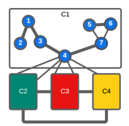
(a) Initial community structure with $4$ communities

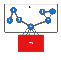
(b) After few iterations, $C2$, $C3$, and $C4$ merge

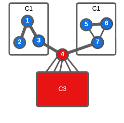
(c) Subsequently, vertex $4$ moves to $C3$

Figure 1. An example demonstrating the possibility of internally disconnected communities with the Louvain algorithm. Here, $C1$, $C2$, $C3$, and $C4$ are four communities obtained after running a few iterations of the Louvain algorithm, with vertices $1$ to $9$ being members of community $C1$. Thick lines are used to denote higher edge weights.

The Louvain method, though effective, has been noted to potentially identify internally disconnected communities (Traag et al., 2019). This is illustrated with an example in Figure 1. Figure 1(a) shows the initial community structure after running a few iterations of the Louvain algorithm. It includes four communities labeled $C1$, $C2$, $C3$, $C4$, and vertices $1$ to $7$ are grouped in community $C1$. After a few additional iterations, in Figure 1(b), communities $C2$, $C3$, and $C4$ merge together into $C3$, due to strong connections among themselves. As vertex $4$ is now more strongly connected to community $C3$, it shifts from community $C1$ to join community $C3$ instead, in Figure 1(c). This results in the internal disconnection of community $C1$, as vertices $1$, $2$, $3$, $5$, $6$, and $7$ retain their locally optimal assignments. Additionally, once all nodes are optimally assigned, the algorithm aggregates the graph. If an internally disconnected community becomes a node in the aggregated graph, it remains disconnected unless it combines with another community acting as a bridge. With subsequent passes, these disconnected communities are prone to steering the solution towards a lower local optima.

3.5. Leiden algorithm

The Leiden algorithm, proposed by Traag et al. (Traag et al., 2019), is a multi-level community detection technique that extends the Louvain method. It consists of three key phases. In the local-moving phase, each vertex $i$ optimizes its community assignment by greedily selecting to join the community of one of its neighbors $j\in J_{i}$, aiming to maximize the modularity gain $\Delta Q_{i:C_{i}\rightarrow C_{j}}$, as defined by Equation 2, akin to the Louvain method. During the refinement phase, vertices within each community undergo further updates to their community memberships, starting from singleton partitions. Unlike the local-moving phase however, these updates are not strictly greedy. Instead, vertices may move to any community within their bounds where the modularity increases, with the probability of joining a neighboring community proportional to the delta-modularity of the move. The level of randomness in these moves is governed by a parameter $\theta>0$. This randomized approach facilitates the identification of higher quality sub-communities within the communities established during the local-moving phase. Finally, in the aggregation phase, all vertices within each refined partition are combined into super-vertices, with an initial community assignment derived from the local-moving phase (Traag et al., 2019). The time complexity of the Leiden algorithm is $O(L|E|)$, where $L$ represents the total number of iterations performed, and its space complexity is $O(|V|+|E|)$.

3.6. Possibility of Internally-disconnected communities with the Leiden algorithm

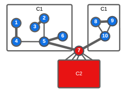
(a) Community $C1$ is internally disconnected

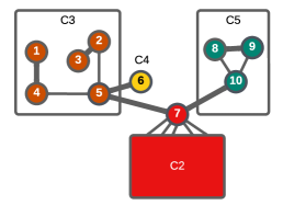
(b) Upon refinement $C1$ splits into $C3$, $C4$, and $C5$

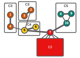
(c) With further refinement, vertex $5$ joins $C4$

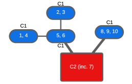
(d) Upon aggregation, if the community assignment for refined partitions is based on the local-moving phase, the community $C1$ is still disconnected

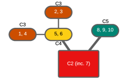
(e) Upon aggregation, if the community assignment for refined partitions is based on the refinement phase, the community $C3$ remains disconnected

Figure 2. An example demonstrating the possibility of internally disconnected communities with the Leiden algorithm. Here, $C1$ and $C2$ are two communities obtained after running some iterations of the Louvain algorithm, where the community $C1$ is internally disconnected — similar to the scenario in Figure 1(c). Vertices $1$ to $6$ and vertices $8$ to $10$ are members of community $C1$, while the vertex $7$ has joined the community $C2$, after having acted as a bridge for $C1$. Upon performing the refinement phase, the community $C1$ splits into communities $C3$, $C4$, and $C5$ after a few iterations (starting from singleton partitions). In a subsequent iteration, suppose vertex $5$ leaves $C3$, and joins $C4$ instead. This causes the $C3$ to be internally disconnected. Finally, (d) and (e) present how disconnected communities continue to persist, depending upon how the community assignments for super-vertices are made (with (d) being the recommended approach by Traag et al. (Traag et al., 2019)). In the figure, ellipses are used to indicate super-vertices in the aggregated graph, and thick lines are used to denote higher edge weights.

We now demonstrate the potential for the Leiden algorithm to produce disconnected communities through an example, shown in Figure 2. In Figure 2(a), $C1$ and $C2$ are two communities obtained after the local-moving phase, with $C1$ being internally disconnected due to vertex $7$ joining community $C2$ — mirroring the scenario depicted in Figure 1(c). Subsequently, the Leiden algorithm performs the refinement phase to rectify disconnected communities. After a few iterations of refinement, community $C1$ may bifurcate into three distinct communities, namely $C3$, $C4$, and $C5$ (see Figure 2(b)).

Note that the refinement phase operates by iteratively optimizing or “refining” partitions via local moves constrained within the boundaries of communities obtained from the local-moving phase. Consequently, it ensures the resolution of the existing disconnected communities, but is not guaranteed to avoid generating any additional disconnected communities within these boundaries. Thus, through further iterations of the refinement phase, vertex $5$ might join community $C4$, resulting in internal disconnection within community $C3$ — as shown in Figure 2(c).

Now, if the community assignments to partitions obtained from the refinement phase are based on the local-moving phase, as suggested by Traag et al. (Traag et al., 2019), community $C1$ still remains disconnected, as depicted in Figure 2(d). This issue may only get resolved if it combines with another community acting as a bridge, such as $C2$. Conversely, if the community assignments are based on the refinement phase itself, community $C3$ stays disconnected (see Figure 2(e)), and may only be resolved if it merges with a bridging community — like $C4$. Thus, the Leiden algorithm does not guarantee the absence of disconnected communities. We observe this empirically in Section 5.2 (Figure 7(d)).

4. Approach

In preceding sections, we explored how both the Louvain and Leiden algorithms can produce internally-disconnected communities. However, this phenomenon is not exclusive to these algorithms and has been documented in various other community detection algorithms (Raghavan et al., 2007; Gregory, 2010; Hesamipour et al., 2022; Ball et al., 2011; Hafez et al., 2014). To mitigate this issue, a commonly employed approach involves splitting disconnected communities as a post-processing step (Raghavan et al., 2007; Gregory, 2010; Hafez et al., 2014; Luecken, 2016; Wolf et al., 2019), utilizing Breadth First Search (BFS) (Raghavan et al., 2007; Gregory, 2010). We refer to this as Split Last (SL) using BFS, or SL-BFS. However, this strategy may exacerbate the problem of poorly connected communities for multi-level community detection techniques, such as the Louvain and Leiden algorithms (Traag et al., 2019).

4.1. Our Split Pass (SP) approach

To tackle the aforementioned challenges encountered by the Leiden and Louvain algorithms, we propose to split the disconnected communities in every pass. Specifically, this occurs after the refinement phase in the Leiden algorithm and following the local-moving phase in the Louvain algorithm. We refer to this as the Split Pass (SP) approach. Additionally, we explore the conventional approach of splitting disconnected communities as a post-processing step, i.e., after all iterations of the community detection algorithm have been completed and the vertex community memberships have converged. This traditional approach is referred to as Split Last (SL).

In order to partition disconnected communities using either the SP or the SL approach, we explore three distinct techniques: minimum-label-based Label Propagation (LP), minimum-label-based Label Propagation with Pruning (LPP), and Breadth First Search (BFS). The rationale behind investigating LP and LPP techniques for splitting disconnected communities as they are readily parallelizable.

With the LP technique, each vertex in the graph initially receives a unique label (its vertex ID). Subsequently, in each iteration, every vertex selects the minimum label among its neighbors within its assigned community, as determined by the community detection algorithm. This iterative process continues until labels for all vertices converge. Since each vertex obtains a unique label within its connected component and its community, communities comprising multiple connected components get partitioned. In contrast, the LPP technique incorporates a pruning optimization step where only unprocessed vertices are handled. Once a vertex is processed, it is marked as such, and gets reactivated (or marked as unprocessed) if one of its neighbors changes their label. The pseudocode for the LP and LPP techniques is presented in Algorithm 1, with detailed explanations given in Section 4.1.1.

On the other hand, the BFS technique for splitting internally-disconnected communities involves selecting a random vertex within each community and identifying all vertices reachable from it as part of one subcommunity. If any vertices remain unvisited in the original community, another random vertex is chosen from the remaining set, and the process iterates until all vertices within each community are visited. Consequently, the BFS technique facilitates the partitioning of connected components within each community. The pseudocode for the BFS technique for splitting disconnected communities is outlined in Algorithm 2, with its in-depth explanation provided in Section 4.1.2.

4.1.1. Explanation of LP/LPP algorithm

We now discuss the pseudocode for the parallel minimum-label-based Label Propagation (LP) and Label Propagation with Pruning (LPP) techniques, given in Algorithm 1, that partition the internally-disconnected communities. These techniques can be employed either as a post-processing step (SL) at the end of the community detection algorithm, or after the refinement/local-moving phase (SP) in each pass. Here, the function splitDisconnectedLp() that is responsible for this task, takes as input the graph $G(V,E)$ and the community memberships $C$ of vertices, and returns the updated community memberships $C^{\prime}$ where all disconnected communities have been separated.

In lines 8-11, the algorithm starts by initializing the minimum labels $C^{\prime}$ of each vertex to their respective vertex IDs, and designates all vertices as unprocessed. Lines 12-29 represent the iteration loop of the algorithm. Initially, the number of changed labels $\Delta N$ is initialized (line 13). This is followed by an iteration of label propagation (lines 14-27), and finally a convergence check (line 29). During each iteration (lines 14-27), unprocessed vertices are processed in parallel. For each unprocessed vertex $i$, it is marked as processed if the Label Propagation with Pruning (LPP) technique is utilized. The algorithm proceeds to identify the minimum label $c^{\prime}_{min}$ within the community of vertex $i$ (lines 18-21). This is achieved by iterating over the outgoing neighbors of $i$ in the graph $G$ and considering only those neighbors belonging to the same community as $i$. The minimum label found among these neighbors, along with the label of vertex $i$ itself, determines the minimum community label $c^{\prime}_{min}$ for $i$. If the obtained minimum label $c^{\prime}_{min}$ differs from the current minimum label $C^{\prime}[i]$ (line 22), $C^{\prime}[i]$ is updated, $\Delta N$ is incremented to reflect the change, and neighboring vertices of $i$ belonging to the same community as $i$ are marked as unprocessed to facilitate their reassessment in subsequent iterations. The label propagation loop (lines 12-29) continues until there are no further changes in the minimum labels. Finally, the updated labels $C^{\prime}$, representing the updated community membership of each vertex with no disconnected communities, are returned in line 30.

Algorithm 1 Split disconnected communities using (min) LP.

1:$G(V,E)$: Input graph

2:$C$: Initial community membership/label of each vertex

3:$C^{\prime}$: Updated community membership/label of each vertex

4:$c^{\prime}_{min}$: Minimum connected label within the community

5:$\Delta N$: Number of changes in labels

6:

7:function splitDisconnectedLp($G,C$)

8:     $C^{\prime}\leftarrow\{\}$

9:     for all $i\in V$ in parallel do

10:         Mark $i$ as unprocessed

11:         $C^{\prime}[i]=i$      

12:     loop

13:         $\Delta N\leftarrow 0$

14:         for all unprocessed $i\in V$ in parallel do

15:              if is SL-LPP or SP-LPP then

16:                  Mark $i$ as processed               

17:              $\rhd$ Find minimum community label

18:              $c^{\prime}_{min}\leftarrow C^{\prime}[i]$

19:              for all $j\in G.out(i)$ do

20:                  if $C[j]=C[i]$ then

21:                       $c^{\prime}_{min}\leftarrow min(C^{\prime}[j],c^{\prime}_{min})$                                 

22:              if $c^{\prime}_{min}=C^{\prime}[i]$ then continue               

23:              $\rhd$ Update community label

24:              $C^{\prime}[i]\leftarrow c^{\prime}_{min}$ ; $\Delta N\leftarrow\Delta N+1$

25:              if is SL-LPP or SP-LPP then

26:                  for all $j\in G.out(i)$ do

27:                       Mark $j$ as unprocessed if $C[j]=C[i]$                                           

28:         $\rhd$ Converged?

29:         if $\Delta N=0$ then break               

30:     return $C^{\prime}$

4.1.2. Explanation of BFS algorithm

Next, we proceed to describe the pseudocode of the parallel Breadth First Search (BFS) technique, as presented in Algorithm 2, devised for the partitioning of disconnected communities. As with LP/LPP techniques, this technique can be applied either as a post-processing step (SL) at the end or after the refinement or local-moving phase (SP) in each pass. Here, the function splitDisconnectedBfs() accepts the input graph $G(V,E)$ and the community membership $C$ of each vertex, and returns the updated community membership $C^{\prime}$ of each vertex where all the disconnected communities have been split.

Initially, in lines 10-12, the flag vector $vis$ representing visited vertices is initialized, and the labels $C^{\prime}$ for each vertex are set to their corresponding vertex IDs. Subsequently, each thread concurrently processes every vertex $i$ in the graph $G$ (lines 14-19). If the community $c$ of vertex $i$ is not present in the work-list $work_{t}$ of the current thread $t$, or if vertex $i$ has been visited, the thread proceeds to the next iteration (line 16). Conversely, if community $c$ is in the work-list $work_{t}$ of the current thread $t$ and vertex $i$ has not been visited, a BFS is performed from vertex $i$ to explore vertices within the same community. This BFS utilizes lambda functions $f_{if}$ to selectively execute BFS on vertex $j$ if it belongs to the same community, and $f_{do}$ to update the label of visited vertices after each vertex is explored during BFS (line 19). Upon completion of processing all vertices, threads synchronize, and the revised labels $C^{\prime}$ — representing the updated community membership of each vertex with no disconnected communities — are returned (line 20). It is pertinent to note that the work-list $work_{t}$ for each thread identified by $t$ is defined as a set encompassing communities $[t\chi,\ t(\chi+1))\ \cup\ [T\chi+t\chi,\ T\chi+t(\chi+1))\ \cup\ \ldots$, where $\chi$ denotes the chunk size, and $T$ signifies the total number of threads. In our implementation, a chunk size of $\chi=1024$ is employed.

Algorithm 2 Split disconnected communities using BFS.

1:$G(V,E)$: Input graph

2:$C$: Initial community membership/label of each vertex

3:$C^{\prime}$: Updated community membership/label of each vertex

4:$f_{if}$: Perform BFS to vertex $j$ if condition satisfied

5:$f_{do}$: Perform operation after each vertex is visited

6:$vis$: Visited flag for each vertex

7:$work_{t}$: Work-list of current thread

8:

9:function splitDisconnectedBfs($G,C$)

10:     $C^{\prime}\leftarrow\{\}$ ; $vis\leftarrow\{\}$

11:     for all $i\in V$ in parallel do

12:         $C^{\prime}[i]=i$      

13:     for all threads do

14:         for all $i\in V$ do

15:              $c^{\prime}\leftarrow C^{\prime}[i]$

16:              if $c\notin work_{t}$ or $vis[i]$ then continue               

17:              $f_{if}\leftarrow(j)\implies C[j]=C[j]$

18:              $f_{do}\leftarrow(j)\implies C^{\prime}[j]\leftarrow c^{\prime}$

19:              $bfsVisitForEach(vis,G,i,f_{if},f_{do})$                

20:     return $C^{\prime}$

Figure 3 illustrates an example of the BFS technique. Initially, Figure 3(a) displays two communities, $C1$ and $C2$, derived after the local-moving phase. Here, $C1$ has become internally disconnected due to the inclusion of vertex $4$ into community $C2$ — similar to the case depicted in Figure 1(c). Subsequently, employing the BFS technique, a thread selects a random vertex within community $C1$, such as $2$, and designates all vertices reachable within $C1$ from $2$ with the label of $2$, and marking them as visited (Figure 3(b)). Following this, as depicted in Figure 3(c), the same thread picks an unvisited vertex randomly within community $C1$, for example, $7$, and labels all vertices reachable within $C1$ from $7$ with the label of $7$, and marking them as visited. An analogous process is executed within community $C2$. Consequently, all vertices are visited, and the labels assigned to them denote the updated community membership of each vertex with no disconnected communities. Note that each thread has a mutually exclusive work-list, ensuring that two threads do not simultaneously perform BFS within the same community.

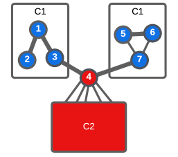
(a) Community $C1$ is internally disconnected

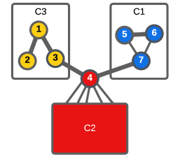
(b) After BFS relabeling from vertex $2$

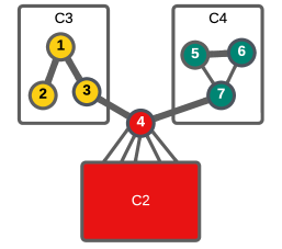
(c) After BFS relabeling from vertex $7$

Figure 3. An example illustrating the BFS technique for splitting internally-disconnected communities. Initially, two communities, $C1$ and $C2$, are shown, with $C1$ being internally disconnected due to vertex $4$ joining $C2$. The BFS technique selects random vertices within each community and labels reachable vertices with the same label, indicated with a new community ID.

4.2. Our GSP-Leiden algorithm

To evaluate our SP approach and the conventional SL approach — employing LP, LPP, and BFS techniques for partitioning disconnected communities with the Leiden algorithm — we use GVE-Leiden, our parallel implementation of the Leiden algorithm (Sahu, 2023a).

4.2.1. Determining suitable configuration for Parallel Leiden

Our first objective is to determine an appropriate configuration for GVE-Leiden that minimizes the occurrence of disconnected communities and maximizes modularity, while still maintaining satisfactory runtime performance. For this, we investigate three variants of GVE-Leiden: light, medium, and heavy.

In the light variant of GVE-Leiden, we adopt the default configuration parameters, including a start tolerance $\tau$ of $10^{-2}$, an aggregation tolerance $\tau_{agg}$ of $0.8$ to prevent aggregations that merge only a small number of communities, enable threshold scaling optimization with a $TOLERANCE\_DROP$ value of $10$, a maximum of $20$ iterations per pass, and a maximum of $10$ passes (Sahu, 2023a). With the medium variant of GVE-Leiden, we set the start tolerance $\tau$ to $10^{-6}$, disable aggregation optimization ($\tau_{agg}=1$), and restrict the maximum iterations per pass and the maximum passes to $100$. Lastly, in the heavy variant of GVE-Leiden, we additionally disable threshold scaling optimization ($TOLERANCE\_DROP=1$).

Figures 4(a), 4(b), and 4(c) show the mean relative runtime, modularity, and fraction of disconnected communities utilizing the light, medium, and greedy variants of GVE-Leiden across all graphs in the dataset (see Section 5.1.3 and Table 1). Additionally, we include results for GVE-Louvain (Sahu, 2023b), our parallel implementation of the Louvain algorithm, for reference. As Figures 4(c) and 4(b) show, the heavy variant of GVE-Leiden achieves the lowest fraction of disconnected communities (approximately $3\times$ lower than communities obtained with the light variant of GVE-Leiden) while also achieving the highest modularity (equivalent to the medium variant of GVE-Leiden). Furthermore, as shown in Figure 4(a), the heavy variant of GVE-Leiden does not have a significantly higher runtime than the medium variant of GVE-Leiden. Note that the heavy variant of GVE-Leiden performs more iterations of the Leiden algorithm (with a greedy refinement phase), and is thus likely to find (more) well connected communities, in addition to obtaining fewer disconnected communities intrinsically. We therefore select the heavy variant of GVE-Leiden for identifying connected communities.

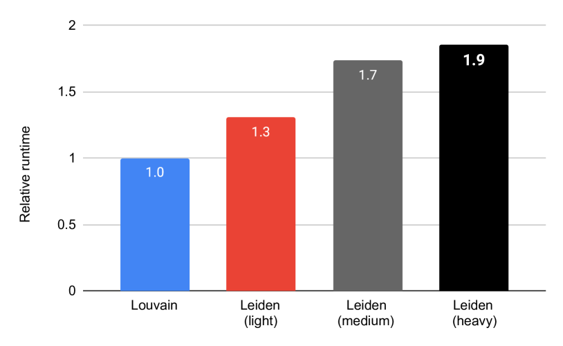
(a) Relative runtime for Parallel Louvain algorithm, and light, medium, and heavy variants of Parallel Leiden algorithm

(b) Modularity of communities obtained for Parallel Louvain algorithm, and light, medium, and heavy variants of Parallel Leiden algorithm

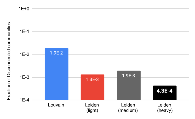
(c) Fraction of disconnected communities for Parallel Louvain algorithm, and light, medium, and heavy variants of Parallel Leiden algorithm

Figure 4. Mean relative runtime, modularity, and fraction of disconnected communities using the light, medium, and greedy variants of Parallel Leiden algorithm (Sahu, 2023a) across all graphs in the dataset. Additionally, details for Parallel Louvain algorithm (Sahu, 2023b) are included as a reference.

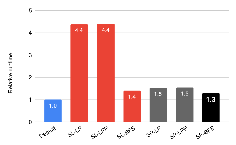
(a) Relative runtime using different approaches for splitting disconnected communities with Parallel Leiden algorithm

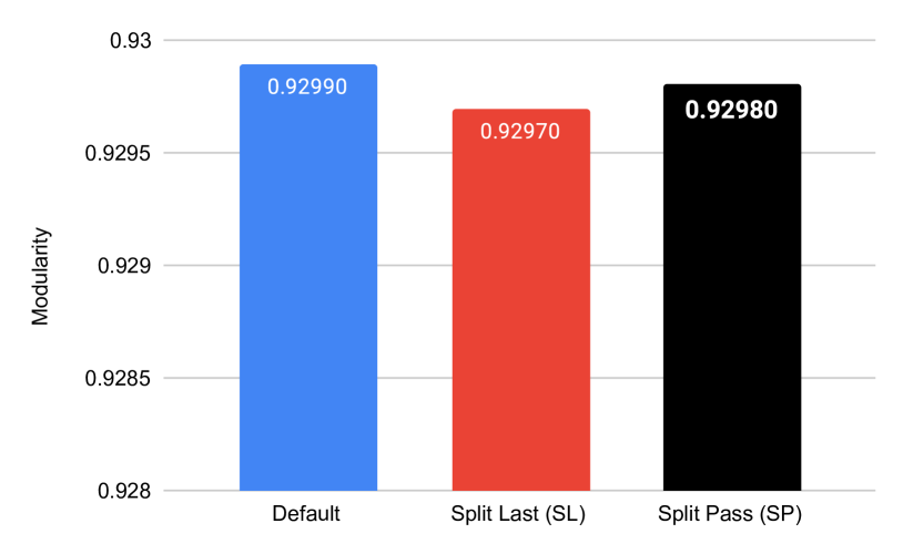
(b) Modularity of communities obtained using different approaches for splitting disconnected communities with Parallel Leiden algorithm

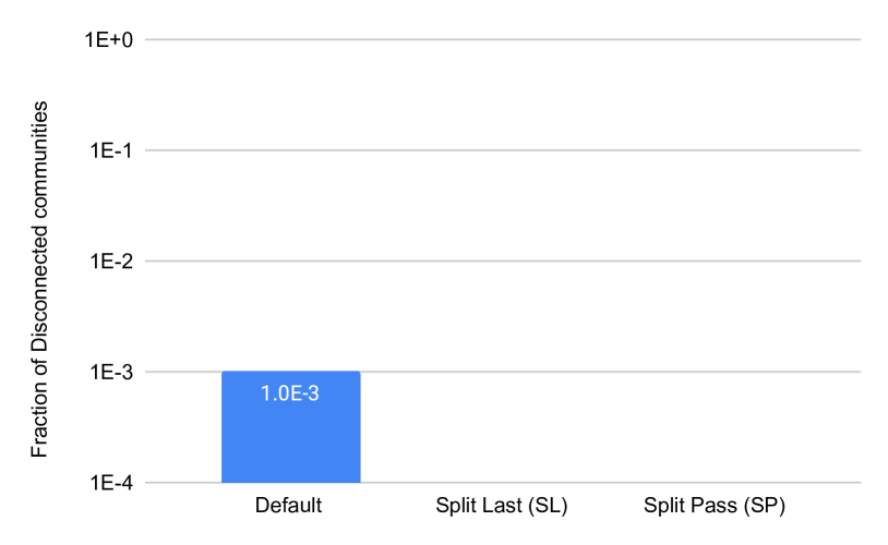
(c) Fraction of disconnected communities (logarithmic scale) using different approaches for splitting disconnected communities with Parallel Leiden algorithm

Figure 5. Mean relative runtime, modularity, and fraction of disconnected communities (log-scale) using Split Last (SL) and Split Pass (SP) approaches for splitting disconnected communities with Parallel Leiden algorithm (Sahu, 2023a) across all graphs in the dataset. Both SL and SP approaches employ Label Propagation (LP), Label Propagation with Pruning (LPP), or Breadth First Search (BFS) techniques for splitting.

4.2.2. Determining suitable technique for splitting disconnected communities

We now determine a suitable technique for partitioning internally-disconnected communities using GVE-Leiden. To accomplish this, we explore both the Split Last (SL) and the Split Pass (SP) approaches employing minimum-label-based Label Propagation (LP), minimum-label-based Label Propagation with Pruning (LPP), and Breadth First Search (BFS) techniques. Figures 5(a), 5(b), and 5(c) present the mean relative runtime, modularity, and fractions of disconnected communities for SL-LP, SL-LPP, SL-BFS, SP-LP, SP-LPP, SP-BFS, and the default (i.e., not splitting disconnected communities) approaches. From Figure 5(c), it is evident that both SL and SP approaches yield non-disconnected communities. Figure 5(b) indicates that the modularity of communities obtained via the SP approach surpasses that of the SL approach while remaining comparable to the default approach. Lastly, Figure 5(a) demonstrates that SP-BFS, i.e., the SP approach employing the BFS technique, exhibits the best performance. Thus, employing BFS to split disconnected communities in each pass (SP) of the Leiden algorithm emerges as the preferred choice.

4.2.3. Explanation of the algorithm

We refer to the heavy variant of GVE-Leiden, which uses the SP-BFS approach for splitting disconnected communities, as GSP-Leiden. The psuedocode for the main step of our parallel GSP-Leiden (leiden() function) is given in Algorithm 3, encompassing initialization, the local-moving phase, the refinement phase, the splitting phase, and the aggregation phase. Here, leiden() accepts the input graph $G$ and outputs the community membership $C$ of each vertex. Initially, in line 12, we initialize the community membership $C$ for each vertex in $G$ and conduct passes of the Leiden algorithm, constrained by $MAX\_PASSES$ (lines 13-25). During each pass, we initialize the total edge weight of each vertex $K^{\prime}$, the total edge weight of each community $\Sigma^{\prime}$, and the community membership $C^{\prime}$ of each vertex in the current graph $G^{\prime}$.

Algorithm 3 GSP-Leiden: Our Parallel Leiden algorithm which returns communities that are not internally disconnected.

1:$G(V,E)$: Input graph

2:$G^{\prime}(V^{\prime},E^{\prime})$: Input/super-vertex graph

3:$C$: Community membership of each vertex

4:$C^{\prime}$: Community membership of each vertex in $G^{\prime}$

5:$K^{\prime}$: Total edge weight of each vertex

6:$\Sigma^{\prime}$: Total edge weight of each community

7:$l_{i}$, $l_{j}$: Number of iterations performed (per pass)

8:$l_{p}$: Number of passes performed

9:$\tau,\tau_{agg}$: Iteration, Aggregation tolerance

10:

11:function leiden($G$)

12:     Vertex membership: $C\leftarrow[0..|V|)$ ; $G^{\prime}\leftarrow G$

13:     for all $l_{p}\in[0..\text{\small{MAX\_PASSES}})$ do

14:         $\Sigma^{\prime}\leftarrow K^{\prime}\leftarrow vertexWeights(G^{\prime})$ ; $C^{\prime}\leftarrow[0..|V^{\prime}|)$

15:         $l_{i}\leftarrow commonMove(G^{\prime},C^{\prime},K^{\prime},\Sigma^{\prime},\tau)$ $\triangleright$ Algorithm 5

16:         $C^{\prime}_{B}\leftarrow C^{\prime}$ ; $C^{\prime}\leftarrow[0..|V^{\prime}|)$ ; $\Sigma^{\prime}\leftarrow K^{\prime}$

17:         $l_{j}\leftarrow leidenRefine(G^{\prime},C^{\prime}_{B},C^{\prime},K^{\prime},\Sigma^{\prime},\tau)$ $\triangleright$ Algorithm 6

18:         $C^{\prime}\leftarrow splitDisconnectedBfs(G^{\prime},C^{\prime})$ $\triangleright$ Algorithm 2

19:         if $l_{i}+l_{j}\leq 1$ then break $\triangleright$ Globally converged?          

20:         $|\Gamma|,|\Gamma_{old}|\leftarrow$ Number of communities in $C$, $C^{\prime}$

21:         if $|\Gamma|/|\Gamma_{old}|>\tau_{agg}$ then break $\triangleright$ Low shrink?          

22:         $C^{\prime}\leftarrow$ Renumber communities in $C^{\prime}$

23:         $C\leftarrow$ Lookup dendrogram using $C$ to $C^{\prime}$

24:         $G^{\prime}\leftarrow commonAggregate(G^{\prime},C^{\prime})$ $\triangleright$ Algorithm 7

25:         $\tau\leftarrow\tau/\text{\small{TOLERANCE\_DROP}}$ $\triangleright$ Threshold scaling      

26:     $C\leftarrow$ Lookup dendrogram using $C$ to $C^{\prime}$

27:     return $C$

Subsequently, in line 15, the local-moving phase is executed by invoking commonMove() (Algorithm 5), optimizing community assignments. Following this, the community bound of each vertex is set (for the refinement phase) as the community membership of each vertex just obtained. We then reset the membership of each vertex and the total weight of each community as singleton vertices in line 16. The refinement phase is conducted in line 17 by invoking leidenRefine() (Algorithm 6), which optimizes the community assignment of each vertex within its community bound. We then split the disconnected communities in parallel with BFS (line 18), using the splitCommunitiesBfs() function (Algorithm 2). If either the local-moving or the refinement phase converges in a single iteration, global convergence is inferred, and we terminate the passes (line 19). Additionally, if the drop in community count $|\Gamma|$ is marginal, the current pass is halted (line 21).

In case convergence is not achieved, we proceed to renumber communities (line 22), update top-level community memberships $C$ with dendrogram lookup (line 23), execute the aggregation phase by calling commonAggregate() (Algorithm 7), and adjust the convergence threshold for subsequent passes, i.e., perform threshold scaling (line 25). The next pass commences in line 13. Following all passes, a final update of the top-level community memberships $C$ with dendrogram lookup is performed (line 26), and the top-level community membership $C$ of each vertex in $G$ is returned.

Detailed explanation of local-moving phase, refinement phase, splitting phase, and the aggregation phase of GSP-Leiden is given in Sections A.1.1, A.1.2, 4.1.2, and A.1.3 respectively.

4.3. Our GSP-Louvain algorithm

To assess both our Split Pass (SP) approach and the conventional Split Last (SL) approach, utilizing minimum-label-based Label Propagation (LP), minimum-label-based Label Propagation with Pruning (LPP), and Breadth First Search (BFS) techniques for splitting disconnected communities with the Louvain algorithm, we use GVE-Louvain (Sahu, 2023b), our parallel implementation of Louvain algorithm.

4.3.1. Determining suitable technique for splitting disconnected communities

We now determine the optimal technique for partitioning internally-disconnected communities using GVE-Louvain. To achieve this, we investigate both the SL and SP approaches, employing LP, LPP, and BFS techniques. Figures 6(a), 6(b), and 6(c) illustrate the mean relative runtime, modularity, and fractions of disconnected communities for SL-LP, SL-LPP, SL-BFS, SP-LP, SP-LPP, SP-BFS, and the default (i.e., not splitting disconnected communities) approaches. As depicted in Figure 6(c), both SL and SP approaches result in non-disconnected communities. Additionally, Figure 6(b) reveals that the modularity of communities obtained through the SP approach surpasses that of the SL approach while maintaining proximity to the default approach. Finally, Figure 6(a) illustrates that SP-BFS, specifically the SP approach employing the BFS technique, demonstrates superior performance. Consequently, employing BFS to split disconnected communities in each pass (SP) of the Louvain algorithm emerges as the preferred choice.

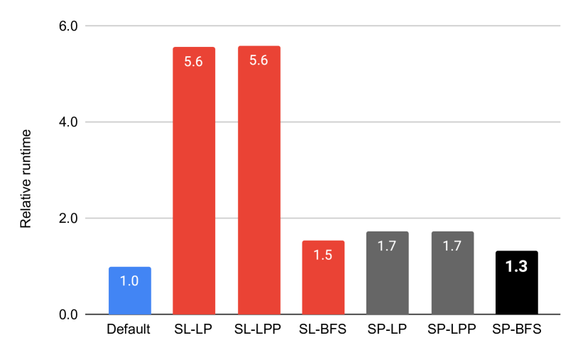
(a) Relative runtime using different approaches for splitting disconnected communities with Parallel Louvain algorithm

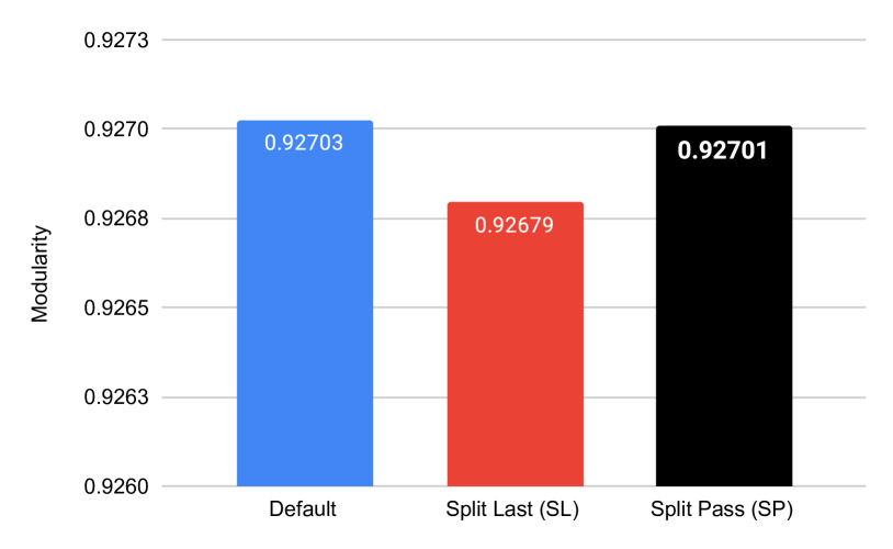
(b) Modularity using different approaches for splitting disconnected communities with Parallel Louvain algorithm

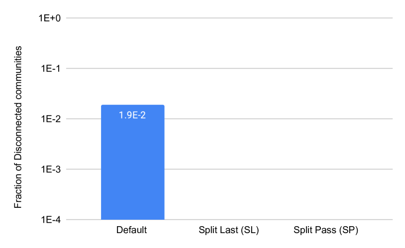
(c) Fraction of disconnected communities (logarithmic scale) using different approaches for splitting disconnected communities with Parallel Louvain algorithm

Figure 6. Mean relative runtime, modularity, and fraction of disconnected communities (log-scale) using Split Last (SL) and Split Pass (SP) approaches for splitting disconnected communities with Parallel Louvain algorithm (Sahu, 2023a) across all graphs in the dataset. Both SL and SP approaches employ Label Propagation (LP), Label Propagation with Pruning (LPP), or Breadth First Search (BFS) techniques for splitting.

4.3.2. Explanation of the algorithm

We refer to GVE-Louvain, which employs the Split Pass (SP) approach with Breadth-First Search (SP-BFS) technique to handle disconnected communities, as GSP-Louvain. The core procedure of GSP-Louvain, encapsulated in the louvain() function, is given in Algorithm 4. It consists of the following main steps: initialization, local-moving phase, splitting phase, and the aggregation phase. This function takes as input a graph $G(V,E)$ and outputs the community membership $C$ for each vertex in the graph, with none of the returned communities being internally disconnected.

First, in line 12, the community membership $C$ is initialized for each vertex in $G$, and the algorithm conducts passes of the Louvain algorithm, limited to a maximum number of passes defined by $MAX\_PASSES$. During each pass, various metrics such as the total edge weight of each vertex $K^{\prime}$, the total edge weight of each community $\Sigma^{\prime}$, and the community membership $C^{\prime}$ of each vertex in the current graph $G^{\prime}$ are updated. Subsequently, in line 16, the local-moving phase is executed by invoking commonMove() (Algorithm 5), which optimizes the community assignments. Following this, the algorithm proceeds to the splitting phase, where the internally disconnected communities in $C^{\prime}$ are separated. This is done using the parallel BFS technique, in line 17, with the splitCommunitiesBfs() function (Algorithm 2). Next, in line 18, global convergence is inferred if the local-moving phase converges in a single iteration. If so, we terminate the passes. Additionally, if there is minimal reduction in the number of communities ($|\Gamma|$), indicating diminishing returns, the current pass is halted (line 20).

If convergence is not achieved, the algorithm proceeds with the following steps: renumbering communities (line 21), updating top-level community memberships $C$ using dendrogram lookup (line 22), executing the aggregation phase via commonAggregate() (Algorithm 7), and adjusting the convergence threshold for subsequent passes, known as threshold scaling (line 24). The subsequent pass initiates at line 13. Upon completion of all passes, a final update of the top-level community memberships $C$ using dendrogram lookup occurs (line 25), followed by the return of the top-level community membership $C$ of each vertex in graph $G$.

Algorithm 4 GSP-Louvain: Our Parallel Louvain algorithm which identifies communities that are not internally disconnected.

1:$G(V,E)$: Input graph

2:$G^{\prime}(V^{\prime},E^{\prime})$: Input/super-vertex graph

3:$C$: Community membership of each vertex

4:$C^{\prime}$: Community membership of each vertex in $G^{\prime}$

5:$K^{\prime}$: Total edge weight of each vertex

6:$\Sigma^{\prime}$: Total edge weight of each community

7:$l_{i}$: Number of iterations performed (per pass)

8:$l_{p}$: Number of passes performed

9:$\tau,\tau_{agg}$: Iteration, Aggregation tolerance

10:

11:function louvain($G$)

12:     Vertex membership: $C\leftarrow[0..|V|)$ ; $G^{\prime}\leftarrow G$

13:     for all $l_{p}\in[0..\text{\small{MAX\_PASSES}})$ do

14:         $\Sigma^{\prime}\leftarrow K^{\prime}\leftarrow vertexWeights(G^{\prime})$ ; $C^{\prime}\leftarrow[0..|V^{\prime}|)$

15:         Mark all vertices in $G^{\prime}$ as unprocessed

16:         $l_{i}\leftarrow commonMove(G^{\prime},C^{\prime},K^{\prime},\Sigma^{\prime},\tau)$ $\triangleright$ Algorithm 5

17:         $C^{\prime}\leftarrow splitDisconnectedBfs(G^{\prime},C^{\prime})$ $\triangleright$ Algorithm 2

18:         if $l_{i}\leq 1$ then break $\triangleright$ Globally converged?          

19:         $|\Gamma|,|\Gamma_{old}|\leftarrow$ Number of communities in $C$, $C^{\prime}$

20:         if $|\Gamma|/|\Gamma_{old}|>\tau_{agg}$ then break $\triangleright$ Low shrink?          

21:         $C^{\prime}\leftarrow$ Renumber communities in $C^{\prime}$

22:         $C\leftarrow$ Lookup dendrogram using $C$ to $C^{\prime}$

23:         $G^{\prime}\leftarrow commonAggregate(G^{\prime},C^{\prime})$ $\triangleright$ Algorithm 7

24:         $\tau\leftarrow\tau/\text{\small{TOLERANCE\_DROP}}$ $\triangleright$ Threshold scaling      

25:     $C\leftarrow$ Lookup dendrogram using $C$ to $C^{\prime}$

26:     return $C$

5. Evaluation

5.1. Experimental Setup

5.1.1. System used

We utilize a server comprising two Intel Xeon Gold 6226R processors, with each processor housing $16$ cores operating at $2.90$ GHz. Each core is equipped with a $1$ MB L1 cache, a $16$ MB L2 cache, and a shared L3 cache of $22$ MB. The system is configured with $376$ GB of RAM and is running CentOS Stream 8.

5.1.2. Configuration

We employ 32-bit integers to represent vertex IDs and 32-bit floats for edge weights, while computations and hashtable values utilize 64-bit floats. We utilize $64$ threads to match the number of available cores on the system, unless stated otherwise. Compilation is performed using GCC 8.5 and OpenMP 4.5.

5.1.3. Dataset

The graphs utilized in our experiments are listed in Table 1, sourced from the SuiteSparse Matrix Collection (Kolodziej et al., 2019). These graphs exhibit $3.07$ to $214$ million vertices, and $25.4$ million to $3.80$ billion edges. We ensure that the edges are undirected and weighted, with a default weight of $1$.

Table 1. List of $13$ graphs obtained SuiteSparse Matrix Collection (Kolodziej et al., 2019) (directed graphs are marked with $*$). Here, $|V|$ is the number of vertices, $|E|$ is the number of edges (after adding reverse edges), $D_{avg}$ is the average degree, and $|\Gamma|$ is the number of communities obtained with GSP-Leiden.

Graph	$|V|$	$|E|$	$D_{avg}$	$|\Gamma|$
Web Graphs (LAW)
indochina-2004∗	7.41M	341M	41.0	4.64K
uk-2002∗	18.5M	567M	16.1	42.5K
arabic-2005∗	22.7M	1.21B	28.2	3.64K
uk-2005∗	39.5M	1.73B	23.7	21.3K
webbase-2001∗	118M	1.89B	8.6	2.78M
it-2004∗	41.3M	2.19B	27.9	5.18K
sk-2005∗	50.6M	3.80B	38.5	3.85K
Social Networks (SNAP)
com-LiveJournal	4.00M	69.4M	17.4	3.97K
com-Orkut	3.07M	234M	76.2	39
Road Networks (DIMACS10)
asia_osm	12.0M	25.4M	2.1	2.38K
europe_osm	50.9M	108M	2.1	3.06K
Protein k-mer Graphs (GenBank)
kmer_A2a	171M	361M	2.1	18.2K
kmer_V1r	214M	465M	2.2	9.48K

5.2. Performance Comparison

We now compare the performance of GSP-Leiden and GSP-Louvain with the original Leiden (Traag et al., 2019), igraph Leiden (Csardi et al., 2006), and NetworKit Leiden (Staudt et al., 2016). For the original Leiden, we employ a C++ program to initialize a ModularityVertexPartition upon the loaded graph and invoke optimise_partition() to determine the community membership of each vertex. In the case of igraph Leiden, we utilize igraph_community_leiden() with a resolution of $1/2|E|$, a beta value of $0.01$, and specify that the algorithm to run until convergence. For NetworKit Leiden, we create a Python script to call ParallelLeiden(), while constraining the number of passes to $10$. For each graph, we measure the runtime of each implementation and the modularity of the resulting communities five times to obtain an average. Additionally, we store the community membership vector in a file and subsequently determine the number of disconnected components using Algorithm 8. Throughout these evaluations, we optimize for modularity as the quality function.

Figure 7(a) presents the runtimes of the original Leiden, igraph Leiden, NetworKit Leiden, GSP-Leiden, and GSP-Louvain on each graph in the dataset. On the sk-2005 graph, GSP-Leiden and GSP-Louvain identify communities in $19.5$ seconds and $11.6$ seconds respectively, achieving a processing rate of $195$ million edges/s and $328$ million edges/s. Figure 7(b) illustrates the speedup of GSP-Leiden and GSP-Louvain relative to the original Leiden. On average, GSP-Leiden and GSP-Louvain exhibit speedups of $190\times$ and $341\times$, respectively, compared to the original Leiden. Furthermore, GSP-Leiden and GSP-Louvain are on average $46\times$ and $83\times$ faster than igraph Leiden, and $3.4\times$ and $6.1\times$ faster than NetworKit Leiden.

Figure 7(c) displays the modularity of communities obtained using each implementation. On average, GSP-Leiden achieves modularity values that are $0.07\%$ and $0.02\%$ lower than those obtained by the original Leiden and igraph Leiden, respectively, but $26\%$ higher than those obtained by NetworKit Leiden (particularly noticeable on road networks and protein k-mer graphs). Similarly, GSP-Louvain achieves modularity values that are, on average, $0.3\%$ lower than those obtained by the original Leiden and igraph Leiden, but $25\%$ higher than those obtained by NetworKit Leiden (again with notable differences on road networks and protein k-mer graphs).

Finally, Figure 7(d) illustrates the fraction of disconnected communities obtained by each implementation. The absence of bars indicates the absence of disconnected communities. As expected, communities identified by GSP-Leiden and GSP-Louvain exhibit no disconnected communities. However, on average, the original Leiden, igraph Leiden, and NetworKit Leiden exhibit fractions of disconnected communities amounting to $1.3\times 10^{-4}$, $7.9\times 10^{-5}$, and $1.5\times 10^{-2}$, respectively, particularly noticeable on web graphs (and especially on social networks for NetworKit Leiden).

Thus, GSP-Leiden and GSP-Louvain effectively tackle the issue of disconnected communities, while being significantly faster than existing alternatives, and attaining similar modularity scores. Between the two, GSP-Leiden achieves communities with an average modularity that is $0.3\%$ higher than that of GSP-Louvain, while GSP-Louvain demonstrates an average speedup of $1.8\times$ compared to GSP-Leiden. Figure 11 depicts the comparison of GVE-Leiden (Sahu, 2023a), GVE-Louvain (Sahu, 2023b), GSP-Leiden, and GSP-Louvain. This comparison is explained in detail in Section A.3.

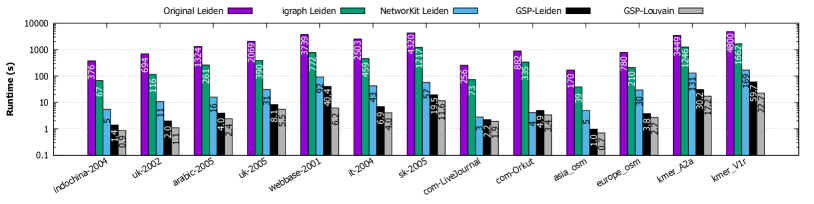
(a) Runtime in seconds (logarithmic scale) with Original Leiden, igraph Leiden, NetworKit Leiden, GSP-Leiden, and GSP-Louvain

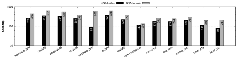
(b) Speedup of GSP-Leiden and GSP-Louvain (logarithmic scale) with respect to Original Leiden.

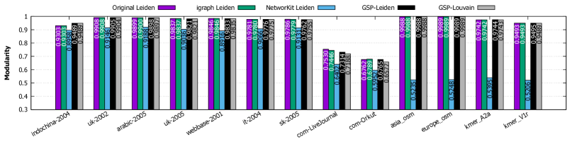
(c) Modularity of communities obtained with Original Leiden, igraph Leiden, NetworKit Leiden, GSP-Leiden, and GSP-Louvain.

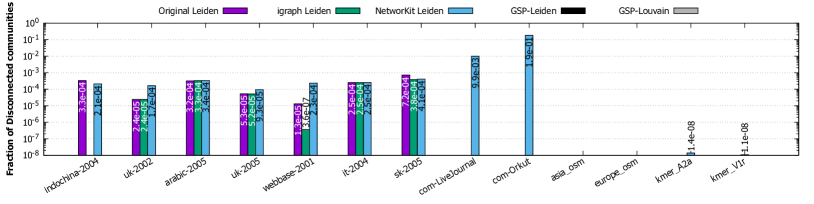
(d) Fraction of disconnected communities (logarithmic scale) with Original Leiden, igraph Leiden, NetworKit Leiden, GSP-Leiden, and GSP-Louvain.

Figure 7. Runtime in seconds (log-scale), speedup (log-scale), modularity, and fraction of disconnected communities (log-scale) with Original Leiden, igraph Leiden, NetworKit Leiden, GSP-Leiden, and GSP-Louvain for each graph in the dataset.

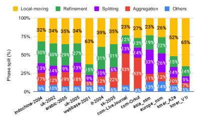
(a) Phase split of GSP-Leiden

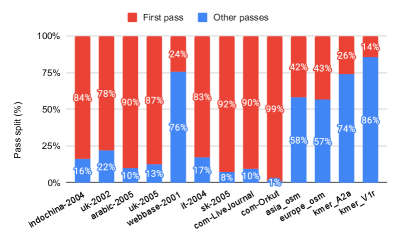
(b) Pass split of GSP-Leiden

Figure 8. Phase split of GSP-Leiden shown on the left, and pass split shown on the right for each graph in the dataset.

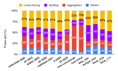
(a) Phase split of GSP-Louvain

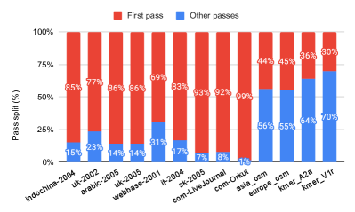
(b) Pass split of GSP-Louvain

Figure 9. Phase split of GSP-Louvain shown on the left, and pass split shown on the right for each graph in the dataset.

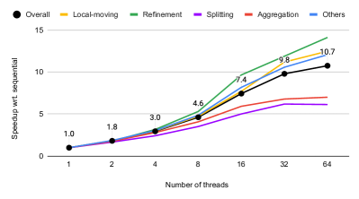
(a) Speedup of GSP-Leiden with respect to sequential

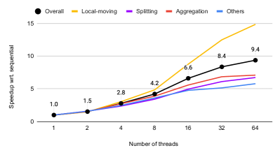
(b) Speedup of GSP-Louvain with respect to sequential

Figure 10. Overall speedup of GSP-Leiden and GSP-Louvain, and their various phases (local-moving, refinement, splitting, aggregation, and others), with increasing number of threads (in multiples of 2).

5.3. Performance Analysis

We proceed to analyze the performance of GSP-Leiden and GSP-Louvain. The phase-wise and pass-wise split of GSP-Leiden is depicted in Figures 8(a) and 8(b), respectively, while that of GSP-Louvain is shown in Figures 9(a) and 9(b), respectively. Figure 8(a) illustrates that GSP-Leiden devotes a considerable portion of its runtime to the local-moving and refinement phases on web graphs, road networks, and protein k-mer graphs, while it predominantly focuses on the aggregation phase on social networks. A notable amount of its runtime is also dedicated to the splitting phase on road networks. Figure 9(a) demonstrates a similar trend for GSP-Louvain, with a majority of the runtime spent in the splitting phase on road networks. The pass-wise breakdown for GSP-Leiden and GSP-Louvain, shown in Figures 8(b) and 9(b), indicates that the initial pass is computationally intensive for high-degree graphs (such as web graphs and social networks), while subsequent passes take precedence in terms of execution time on low-degree graphs (such as road networks and protein k-mer graphs). An exception to this trend is observed on the webbase-2001 graph, where GSP-Leiden primarily spends its runtime in later passes.

On average, GSP-Leiden spends $38\%$ of its runtime in the local-moving phase, $22\%$ in the refinement phase, $14\%$ in the splitting phase, $18\%$ in the aggregation phase, and $8\%$ in other steps (including initialization, renumbering communities, dendrogram lookup, and resetting communities). In contrast, GSP-Louvain dedicates $37\%$ of its runtime to the local-moving phase, $21\%$ to the splitting phase, $29\%$ to the aggregation phase, and $13\%$ to other steps (same as above). Additionally, the first pass of GSP-Leiden consumes $66\%$ of the total runtime, while the first pass of GSP-Louvain accounts for $71\%$ of the total runtime. This initial pass in GSP-Louvain is computationally demanding due to the size of the original graph (subsequent passes operate on super-vertex graphs).

5.4. Strong Scaling

Finally, we evaluate the strong scaling performance of GSP-Leiden and GSP-Louvain by varying the number of threads from $1$ to $64$ (in multiples of $2$) for each input graph. We measure the total time taken for GSP-Leiden and GSP-Louvain to identify communities, with their respective phase splits, including local-moving, refinement (only for GSP-Leiden), splitting, aggregation, and other associated steps. The strong scaling results for GSP-Leiden and GSP-Louvain are illustrated in Figures 10(a) and 10(b), respectively.

With $32$ threads, GSP-Leiden and GSP-Louvain achieve an average speedup of $9.8\times$ and $8.4\times$, respectively, compared to single-threaded execution. This indicates a performance increase of $1.6\times$ and $1.5\times$, respectively, for every doubling of threads. The scalability is limited due to the sequential nature of steps/phases in both algorithms, as well as the lower scalability of splitting and aggregation phases. It is noteworthy that the scalability of GSP-Leiden is higher as it performs more work, requiring more iterations to converge. Consequently, the ”others” phase of GSP-Leiden, which encompasses initialization, renumbering communities, dendrogram lookup, and resetting communities, scales well. At $64$ threads, both GSP-Leiden and GSP-Louvain are impacted by NUMA effects, resulting in speedups of only $10.7\times$ and $9.4\times$, respectively.

6. Conclusion

In this investigation, we presented our analysis and empirical findings, revealing that the Leiden algorithm (Traag et al., 2019) still exhibits tendencies to identify disconnected communities, albeit to a reduced extent. To address this concern, we introduced two new parallel algorithms: GSP-Leiden and GSP-Louvain, which are derived from the Leiden and Louvain algorithms, respectively. Utilizing a system featuring two 16-core Intel Xeon Gold 6226R processors, we demonstrated that GSP-Leiden/GSP-Louvain not only rectify this issue but also achieve an impressive processing rate of $195M$/$328M$ edges/s on a $3.8B$ edge graph. Comparatively, they surpass the original Leiden, igraph Leiden, and NetworKit Leiden by $190\times$/$341\times$, $46\times$/$83\times$, and $3.4\times$/$6.1\times$, respectively. Moreover, the identified communities exhibit similar quality to the first two implementations and are $25\%$ higher in quality than those produced by NetworKit. Additionally, GSP-Leiden/GSP-Louvain exhibit a performance improvement rate of $1.6\times$/$1.5\times$ for every doubling of threads.

Appendix A Appendix

A.1. Phases of GSP-Leiden/GSP-Louvain

Here, we explain the local-moving, refinement (specific to GSP-Leiden), and aggregation phases of GSP-Leiden and GSP-Louvain. For details on the splitting phase, please consult Section 4.1.2.

A.1.1. Local-moving phase of GSP-Leiden/GSP-Louvain

The pseudocode for the local-moving phase of GSP-Leiden/GSP-Louvain is outlined in Algorithm 5. Within this algorithm, vertices are iteratively moved between communities to maximize modularity. The commonMove() function takes as input the current graph $G^{\prime}$, community membership $C^{\prime}$, total edge weight of each vertex $K^{\prime}$ and each community $\Sigma^{\prime}$, and the iteration tolerance $\tau$. It returns the number of iterations performed $l_{i}$.

Lines 11-23 encapsulate the primary loop of the local-moving phase. Initially, all vertices are designated as unprocessed (line 10). Subsequently, in line 12, the total delta-modularity per iteration $\Delta Q$ is initialized. Next, parallel iteration over unprocessed vertices is conducted (lines 13-22). For each unprocessed vertex $i$, $i$ is flagged as processed, i.e., vertex pruning (line 14), followed by scanning communities connected to $i$, excluding itself (line 15). Further, the best community $c^{*}$ for moving $i$ to is determined (line 17), and the delta-modularity $\delta Q^{*}$ of moving $i$ to $c^{*}$ is computed (line 18). If a superior community is identified (with $\delta Q^{*}>0$), the community membership of $i$ is updated (lines 20-21), and its neighbors are marked as unprocessed (line 22). If not, $i$ stays in its original community. Line 23 verifies if the local-moving phase has converged, terminating the loop if so (or if $MAX\_ITERATIONS$ is reached). Finally, in line 24, the number of iterations performed $l_{i}$ is returned.

Algorithm 5 Local-moving phase of GSP-Leiden/GSP-Louvain.

1:$G^{\prime}(V^{\prime},E^{\prime})$: Input/super-vertex graph

2:$C^{\prime}$: Community membership of each vertex

3:$K^{\prime}$: Total edge weight of each vertex

4:$\Sigma^{\prime}$: Total edge weight of each community

5:$\tau$: Iteration tolerance

6:$H_{t}$: Collision-free per-thread hashtable

7:$l_{i}$: Number of iterations performed

8:

9:function commonMove($G^{\prime},C^{\prime},K^{\prime},\Sigma^{\prime},\tau$)

10:     Mark all vertices in $G^{\prime}$ as unprocessed

11:     for all $l_{i}\in[0..\text{\small{MAX\_ITERATIONS}})$ do

12:         Total delta-modularity per iteration: $\Delta Q\leftarrow 0$

13:         for all unprocessed $i\in V^{\prime}$ in parallel do

14:              Mark $i$ as processed (prune)

15:              $H_{t}\leftarrow scanCommunities(\{\},G^{\prime},C^{\prime},i,false)$

16:              $\rhd$ Use $H_{t},K^{\prime},\Sigma^{\prime}$ to choose best community

17:              $c^{*}\leftarrow$ Best community linked to $i$ in $G^{\prime}$

18:              $\delta Q^{*}\leftarrow$ Delta-modularity of moving $i$ to $c^{*}$

19:              if $c^{*}=C^{\prime}[i]$ then continue               

20:              $\Sigma^{\prime}[C^{\prime}[i]]-=K^{\prime}[i]$ ; $\Sigma^{\prime}[c^{*}]+=K^{\prime}[i]$ atomic

21:              $C^{\prime}[i]\leftarrow c^{*}$ ; $\Delta Q\leftarrow\Delta Q+\delta Q^{*}$

22:              Mark neighbors of $i$ as unprocessed          

23:         if $\Delta Q\leq\tau$ then break $\triangleright$ Locally converged?               

24:     return $l_{i}$

25:

26:function scanCommunities($H_{t},G^{\prime},C^{\prime},i,self$)

27:     for all $(j,w)\in G^{\prime}.edges(i)$ do

28:         if not $self$ and $i=j$ then continue          

29:         $H_{t}[C^{\prime}[j]]\leftarrow H_{t}[C^{\prime}[j]]+w$      

30:     return $H_{t}$

A.1.2. Refinement phase of GSP-Leiden

The pseudocode for the refinement phase of GSP-Leiden is presented in Algorithm 5. This phase resembles the local-moving phase but utilizes the obtained community membership of each vertex as a community bound, where each vertex is required to choose to join the community of another vertex within its community bound. At the beginning of the refinement phase, the community membership of each vertex is reset, assigning each vertex to its own community. The leidenRefine() function takes as input the current graph $G^{\prime}$, the community bound of each vertex $C^{\prime}_{B}$, the initial community membership $C^{\prime}$ of each vertex, the total edge weight of each vertex $K^{\prime}$, the initial total edge weight of each community $\Sigma^{\prime}$, and the current per-iteration tolerance $\tau$. It outputs the number of iterations performed $l_{j}$.

Lines 12-24 encapsulate the core functionality of the refinement phase. Initially, all vertices are designated as unprocessed (line 11). Subsequently, the per-iteration delta-modularity $\Delta Q$ is initialized (line 13), followed by parallel iteration over unprocessed vertices (lines 14-23). For each unprocessed vertex $i$, pruning of $i$ is conducted (line 15), communities connected to $i$ within the same community bound are scanned - excluding itself (line 16), the best community $c^{*}$ for moving $i$ to is determined (line 18), and the delta-modularity $\delta Q^{*}$ of moving $i$ to $c^{*}$ is computed (line 19). Upon identifying a superior community, the community membership of $i$ is updated (lines 21-22), and its neighbors are marked as unprocessed (line 23). Line 24 verifies the convergence of the refinement phase, terminating the iterations if so (or if $MAX\_ITERATIONS$ is reached). Finally, the number of iterations performed $l_{j}$ is returned (line 25).

Algorithm 6 Refinement phase of GSP-Leiden.

1:$G^{\prime}(V^{\prime},E^{\prime})$: Input/super-vertex graph

2:$C^{\prime}_{B}$: Community bound of each vertex

3:$C^{\prime}$: Community membership of each vertex

4:$K^{\prime}$: Total edge weight of each vertex

5:$\Sigma^{\prime}$: Total edge weight of each community

6:$\tau$: Iteration tolerance

7:$H_{t}$: Collision-free per-thread hashtable

8:$l_{j}$: Number of iterations performed

9:

10:function leidenRefine($G^{\prime},C^{\prime}_{B},C^{\prime},K^{\prime},\Sigma^{\prime},\tau$)

11:     Mark all vertices in $G^{\prime}$ as unprocessed

12:     for all $l_{j}\in[0..\text{\small{MAX\_ITERATIONS}})$ do

13:         Total delta-modularity per iteration: $\Delta Q\leftarrow 0$

14:         for all unprocessed $i\in V^{\prime}$ in parallel do

15:              Mark $i$ as processed (prune)

16:              $H_{t}\leftarrow scanBounded(\{\},G^{\prime},C^{\prime}_{B},C^{\prime},i,false)$

17:              $\rhd$ Use $H_{t},K^{\prime},\Sigma^{\prime}$ to choose best community

18:              $c^{*}\leftarrow$ Best community linked to $i$ in $G^{\prime}$ within $C^{\prime}_{B}$

19:              $\delta Q^{*}\leftarrow$ Delta-modularity of moving $i$ to $c^{*}$

20:              if $c^{*}=C^{\prime}[i]$ then continue               

21:              $\Sigma^{\prime}[C^{\prime}[i]]-=K^{\prime}[i]$ ; $\Sigma^{\prime}[c^{*}]+=K^{\prime}[i]$ atomic

22:              $C^{\prime}[i]\leftarrow c^{*}$ ; $\Delta Q\leftarrow\Delta Q+\delta Q^{*}$

23:              Mark neighbors of $i$ as unprocessed          

24:         if $\Delta Q\leq\tau$ then break $\triangleright$ Locally converged?               

25:     return $l_{j}$

26:

27:function scanBounded($H_{t},G^{\prime},C^{\prime}_{B},C^{\prime},i,self$)

28:     for all $(j,w)\in G^{\prime}.edges(i)$ do

29:         if not $self$ and $i=j$ then continue          

30:         if $C^{\prime}_{B}[i]\neq C^{\prime}_{B}[j]$ then continue          

31:         $H_{t}[C^{\prime}[j]]\leftarrow H_{t}[C^{\prime}[j]]+w$      

32:     return $H_{t}$

A.1.3. Aggregation phase of GSP-Leiden/GSP-Louvain

Finally, we provide the pseudocode for the aggregation phase in Algorithm 7, which aggregates communities into super-vertices in preparation for the subsequent pass of the Leiden/Louvain algorithm, operating on the super-vertex graph. The commonAggregate() function accepts the current graph $G^{\prime}$ and the community membership $C^{\prime}$ as input and returns the super-vertex graph $G^{\prime\prime}$.

In lines 10-11, the offsets array for the community vertices Compressed Sparse Row (CSR) $G^{\prime}{C^{\prime}}.offsets$ is computed. Initially, this involves determining the number of vertices in each community using countCommunityVertices() and subsequently performing an exclusive scan on the array. Then, in lines 12-13, a parallel iteration over all vertices is conducted to atomically populate vertices belonging to each community into the community graph CSR $G^{\prime}{C^{\prime}}$. Following this, the offsets array for the super-vertex graph CSR is determined by estimating the degree of each super-vertex. This process includes calculating the total degree of each community with communityTotalDegree() and performing an exclusive scan on the array (lines 15-16). As a result, the super-vertex graph CSR exhibits sparsity, with gaps between the edges and weights arrays of each super-vertex in the CSR.

Following that, in lines 18-24, a parallel iteration over all communities $c\in[0,|\Gamma|)$ is executed. For each vertex $i$ belonging to community $c$, all communities $d$ (along with associated edge weight $w$) linked to $i$, as defined by scanCommunities() in Algorithm 5, are included in the per-thread hashtable $H_{t}$. Once $H_{t}$ is populated with all communities (and their associated weights) linked to community $c$, these are atomically added as edges to super-vertex $c$ in the super-vertex graph $G^{\prime\prime}$. Finally, in line 25, the super-vertex graph $G^{\prime\prime}$ is returned.

Algorithm 7 Aggregation phase of GSP-Leiden/GSP-Louvain.

1:$G^{\prime}(V^{\prime},E^{\prime})$: Input/super-vertex graph

2:$C^{\prime}$: Community membership of each vertex

3:$G^{\prime}_{C^{\prime}}(V^{\prime}_{C^{\prime}},E^{\prime}_{C^{\prime}})$: Community vertices (CSR)

4:$G^{\prime\prime}(V^{\prime\prime},E^{\prime\prime})$: Super-vertex graph (weighted CSR)

5:$*.offsets$: Offsets array of a CSR graph

6:$H_{t}$: Collision-free per-thread hashtable

7:

8:function commonAggregate($G^{\prime},C^{\prime}$)

9:     $\rhd$ Obtain vertices belonging to each community

10:     $G^{\prime}_{C^{\prime}}.offsets\leftarrow countCommunityVertices(G^{\prime},C^{\prime})$

11:     $G^{\prime}_{C^{\prime}}.offsets\leftarrow exclusiveScan(G^{\prime}_{C^{\prime}}.offsets)$

12:     for all $i\in V^{\prime}$ in parallel do

13:         Add edge $(C^{\prime}[i],i)$ to CSR $G^{\prime}_{C^{\prime}}$ atomically      

14:     $\rhd$ Obtain super-vertex graph

15:     $G^{\prime\prime}.offsets\leftarrow communityTotalDegree(G^{\prime},C^{\prime})$

16:     $G^{\prime\prime}.offsets\leftarrow exclusiveScan(G^{\prime\prime}.offsets)$

17:     $|\Gamma|\leftarrow$ Number of communities in $C^{\prime}$

18:     for all $c\in[0,|\Gamma|)$ in parallel do

19:         if degree of $c$ in $G^{\prime}_{C^{\prime}}=0$ then continue          

20:         $H_{t}\leftarrow\{\}$

21:         for all $i\in G^{\prime}_{C^{\prime}}.edges(c)$ do

22:              $H_{t}\leftarrow scanCommunities(H,G^{\prime},C^{\prime},i,true)$          

23:         for all $(d,w)\in H_{t}$ do

24:              Add edge $(c,d,w)$ to CSR $G^{\prime\prime}$ atomically               

25:     return $G^{\prime\prime}$

A.2. Finding disconnected communities

We introduce our parallel algorithm designed to identify disconnected communities, given the original graph and the community membership of each vertex. The core principle involves assessing the size of each community, selecting a representative vertex from each community, navigating within the community from that vertex while avoiding neighboring communities, and designating a community as disconnected if all its vertices are unreachable. We investigate four distinct approaches, distinguished by their utilization of parallel Depth-First Search (DFS) or Breadth-First Search (BFS), and whether per-thread or shared visited flags are employed. When shared visited flags are utilized, each thread scans all vertices but exclusively processes its designated community based on the community ID. Our findings reveal that employing parallel BFS traversal with a shared flag vector yields the most efficient results. Given the deterministic nature of this algorithm, all approaches yield identical outcomes. Algorithm 8 outlines the pseudocode for this approach. Here, the disconnectedCommunities() function takes the input graph $G$ and the community membership $C$ as input and returns the disconnected flag $D$ for each community.

Algorithm 8 Finding disconnected communities in parallel (Sahu, 2023a).

1:$G(V,E)$: Input graph

2:$C$: Community membership of each vertex

3:$D$: Disconnected flag for each community

4:$S$: Size of each community

5:$f_{if}$: Perform BFS to vertex $j$ if condition satisfied

6:$f_{do}$: Perform operation after each vertex is visited

7:$reached$: Number of vertices reachable from $i$ to $i$’s community

8:$vis$: Visited flag for each vertex

9:$work_{t}$: Work-list of current thread

10:

11:function disconnectedCommunities($G,C$)

12:     $D\leftarrow\{\}$ ; $vis\leftarrow\{\}$

13:     $S\leftarrow communitySizes(G,C)$

14:     for all threads in parallel do

15:         for all $i\in V$ do

16:              $c\leftarrow C[i]$ ; $reached\leftarrow 0$

17:              $\rhd$ Skip if community $c$ is empty, or

18:              $\rhd$ does not belong to work-list of current thread.

19:              if $S[c]=0$ or $c\notin work_{t}$ then continue               

20:              $f_{if}\leftarrow(j)\implies C[j]=c$

21:              $f_{do}\leftarrow(j)\implies reached\leftarrow reached+1$

22:              $bfsVisitForEach(vis,G,i,f_{if},f_{do})$

23:              if $reached<S[c]$ then $D[c]\leftarrow 1$               

24:              $S[c]\leftarrow 0$                

25:     return $D$

Let us now delve into Algorithm 8. Initially, in line 12, we initialize the disconnected community flag $D$ and the visited vertices flags $vis$. Line 13 computes the size of each community $S$ in parallel using the communitySizes() function. Subsequently, each thread processes each vertex $i$ in the graph $G$ in parallel (lines 15-24). In line 16, we determine the community membership of $i$ ($c$), and set the count of vertices reached from $i$ to $0$. If community $c$ is either empty or not in the work-list of the current thread $work_{t}$, the thread proceeds to the next iteration (line 19). However, if community $c$ is non-empty and in the work-list of the current thread $work_{t}$, we perform BFS from vertex $i$ to explore vertices in the same community. This utilizes lambda functions $f_{if}$ to conditionally execute BFS to vertex $j$ if it belongs to the same community, and $f_{do}$ to update the count of reached vertices after each vertex is visited during BFS (line 22). If the number of vertices $reached$ during BFS is less than the community size $S[c]$, we mark community $c$ as disconnected (line 23). Finally, we update the size of the community $S[c]$ to $0$, indicating that the community has been processed (line 24). It’s important to note that the work-list $work_{t}$ for each thread with ID $t$ is defined as a set containing communities $[t\chi,\ t(\chi+1))\ \cup\ [T\chi+t\chi,\ T\chi+t(\chi+1))\ \cup\ \ldots$, where $\chi$ is the chunk size, and $T$ is the number of threads. In our implementation, we utilize a chunk size of $\chi=1024$.

A.3. Additional Performance comparison

We proceed to compare the performance of GSP-Leiden and GSP-Louvain with GVE-Leiden (Sahu, 2023a) and GVE-Louvain (Sahu, 2023b). Similar to our previous approach, we execute each algorithm five times for every graph in the dataset to mitigate measurement noise and report the averages in Figures 11(a), 11(b), 11(c), and 11(d).

Figure 11(a) illustrates the runtimes of GSP-Leiden, GSP-Louvain, GVE-Leiden, and GVE-Louvain on each graph in the dataset. On average, GSP-Leiden is approximately $83\%$ slower than GVE-Leiden, whereas GSP-Louvain exhibits about a $33\%$ increase in runtime compared to GVE-Louvain. This additional computational time is a compromise made to ensure the absence of internally disconnected communities. Furthermore, GSP-Louvain demonstrates a speed advantage of approximately $1.8\times$ over GSP-Leiden.

Figure 11(c) presents the modularity of communities obtained by each implementation. On average, GSP-Leiden achieves a $0.2\%$ higher modularity than GVE-Leiden, while the modularity of communities obtained using GSP-Louvain and GVE-Louvain remains roughly identical. In the comparison between GSP-Leiden and GSP-Louvain, GSP-Leiden attains communities with an average modularity that is $0.3\%$ higher than that of GSP-Louvain.

Lastly, Figure 11(d) displays the fraction of internally disconnected communities identified by each implementation. Communities obtained with GSP-Leiden and GSP-Louvain exhibit no disconnected communities, whereas communities identified with GVE-Leiden and GVE-Louvain feature on average $1.2\%$ and $3.9\%$ disconnected communities, respectively.

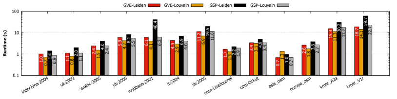
(a) Runtime in seconds (logarithmic scale) with GVE-Leiden, GVE-Louvain, GSP-Leiden, and GSP-Louvain

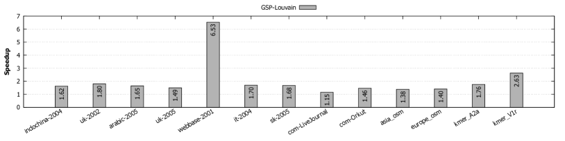
(b) Speedup of GSP-Louvain with respect to GSP-Leiden.

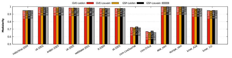
(c) Modularity of communities obtained with GVE-Leiden, GVE-Louvain, GSP-Leiden, and GSP-Louvain.

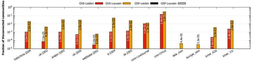
(d) Fraction of disconnected communities (logarithmic scale) with GVE-Leiden, GVE-Louvain, GSP-Leiden, and GSP-Louvain.

Figure 11. Runtime in seconds (log-scale), speedup, modularity, and fraction of disconnected communities (log-scale) with GVE-Leiden, GVE-Louvain, GSP-Leiden, and GSP-Louvain for each graph in the dataset.