Balanced Truncation of Linear Systems with Quadratic Outputs in Limited Time and Frequency Intervals

Abstract

Model order reduction involves constructing a reduced-order approximation of a high-order model while retaining its essential characteristics. This reduced-order model serves as a substitute for the original one in various applications such as simulation, analysis, and design. Often, there’s a need to maintain high accuracy within a specific time or frequency interval, while errors beyond this limit can be tolerated. This paper addresses time-limited and frequency-limited model order reduction scenarios for linear systems with quadratic outputs, by generalizing the recently introduced structure-preserving balanced truncation algorithm [1]. To that end, limited interval system Gramians are defined, and the corresponding generalized Lyapunov equations governing their computation are derived. Additionally, low-rank solutions for these equations are investigated. Next, balanced truncation algorithms are proposed for time-limited and frequency-limited scenarios, each utilizing its corresponding limited-interval system Gramians. The proposed algorithms ensure accurate results within specified time and frequency intervals while preserving the quadratic-output structure. Two benchmark numerical examples are presented to demonstrate the effectiveness of the algorithms, showcasing their ability to achieve superior accuracy within the desired time or frequency interval.

1 Introduction

Mathematical models of both physical and artificial systems and processes are essential for conducting computer simulations, analyses, and related design procedures. With the advancement of chip manufacturing capabilities leading to a decrease in chip size, modern-day computers have witnessed a significant increase in processing and computing power. This enhancement allows for the inclusion of intricate details in the mathematical models of dynamical systems, ensuring high fidelity in computer simulations. However, the addition of more details results in very high-order models, posing computational challenges in simulation and analysis despite the considerable improvement in computer processing power and memory resources. Consequently, design procedures based on these high-order models become complex and sometimes impractical for actual implementation. Hence, there arises a need for a reduced-order approximation of the original high-order model with acceptable numerical error. Model order reduction (MOR) addresses this need by providing a procedure to obtain a reduced-order model (ROM) that accurately approximates the original high-order model while retaining its important properties and characteristics. The specific properties and characteristics to be preserved dictate the algorithmic approach taken by a MOR algorithm to construct a ROM. MOR serves as an effective solution to mitigate the computational costs associated with high-order dynamical models of various practical systems and processes. Refer to [2, 3, 4, 5] for an in-depth exploration of this topic.

Balanced truncation (BT) emerged in 1981 [6] and has since become one of the most widely applied MOR techniques. It selectively retains states associated with significant Hankel singular values while discarding those with minimal contribution to input-output energy transfer. One notable aspect of BT is the availability of an apriori error bound, as derived in [7]. Additionally, BT ensures the stability of the original model. Initially developed for standard first-order linear time-invariant (LTI) systems, BT has undergone significant evolution, expanding its applicability to various classes of systems including descriptor systems [8, 9], second-order systems [10, 11], linear time varying systems [12, 13], parametric systems [14, 15], nonlinear systems [16, 17, 18], and bilinear systems [19, 20], among others, forming a diverse family of algorithms. Furthermore, BT has been extended to preserve system properties such as positive-realness [21], bounded realness [22], passivity [23], and special structures [24, 25], to mention a few. For a comprehensive survey on the BT family of algorithms, refer to [26].

BT typically provides an accurate approximation of the original model across the entire time horizon. However, practical system simulations often operate within limited time intervals, reflecting real-world operational constraints. For example, in interconnected power systems, low-frequency oscillations typically persist for only 15 seconds before being effectively dampened by power system stabilizers and damping controllers [27, 28]. Consequently, the initial 15 seconds play a crucial role in small-signal stability analysis. Similarly, in time-limited optimal control problems [29], the plant’s behavior within the desired time interval is paramount. This necessity drives the concept of time-limited MOR, which prioritizes achieving maximum accuracy within specified time intervals rather than pursuing accuracy across the entire time horizon. To address this, BT was adapted to address the time-limited MOR problem, resulting in the development of a time-limited BT (TLBT) algorithm [30]. Although TLBT does not preserve all BT’s features like stability or an apriori error bound, it effectively addresses the time-limited MOR scenario. Computational aspects of TLBT, along with efficient algorithms for handling large-scale systems, are discussed in [31]. Additionally, TLBT has been extended to a broader class of systems, including descriptor systems [32], second-order systems [33], and bilinear systems [34].

Much like in the time domain, BT typically provides an accurate approximation of the original model across the entire frequency spectrum. Many MOR problems inherently exhibit a frequency-limited nature, as certain frequency intervals hold greater significance. For instance, when constructing a ROM for a notch filter, minimizing the approximation error near the notch frequency becomes paramount [35]. Similarly, to ensure closed-loop stability, the ROM of the plant must effectively capture the system’s behavior in the crossover frequency region [36]. In interconnected power systems, the presence of low-frequency oscillations is critical for small-signal stability studies. Hence, the ROM of interconnected power systems should accurately represent the behavior within the frequency range encompassing inter-area and inter-plant oscillations [37]. This necessity drives the concept of frequency-limited MOR, which prioritizes achieving maximum accuracy within specified frequency intervals rather than pursuing accuracy across the entire frequency spectrum. In [30], BT is extended to address the frequency-limited MOR problem, resulting in the development of a frequency-limited BT (FLBT) algorithm. FLBT, however, does not retain the stability preservation and apriori error bound properties of BT. Computational aspects of FLBT, along with efficient algorithms for handling large-scale systems, are discussed in [38]. Additionally, FLBT has been extended to a more general class of systems, including descriptor systems [39], second-order systems [33], and bilinear systems [40].

LTI systems with quadratic outputs (LTI-QO) constitute an important class of dynamical systems prevalent in various applications. These models emerge in mechanical systems, such as mass-spring-damper systems [41], random vibration analysis [42, 43], and electrical circuits with time-harmonic Maxwell’s equations [44, 45]. Despite the similarity of state equations between LTI-QO systems and standard LTI systems, the output equation of LTI-QO systems is nonlinear, represented by a quadratic function of the states. BT has been extended to accommodate LTI-QO systems, with three main approaches outlined in the literature for generalizing BT. The first approach involves reformulating the LTI-QO system as a standard LTI system and then applying classical BT to derive a ROM [46]. The second approach entails transforming the LTI-QO system into quadratic-bilinear systems and then applying BT’s generalization for bilinear systems to obtain a ROM [47]. However, both of these approaches are computationally demanding and fail to preserve the structure of LTI-QO systems. The third approach employs Hilbert space adjoint theory to define system Gramians for LTI-QO systems. Using these system Gramians, this approach generalizes the BT method to LTI-QO systems [1], ensuring preservation of the system’s structure unlike the previous approaches [46, 47]. Furthermore, the system Gramians are shown to be solutions of generalized Lyapunov equations, which can be efficiently computed using low-rank approximations [48, 49], rendering this approach computationally efficient.

This paper extends the BT algorithm recently introduced for LTI-QO systems in [1] to address time-limited and frequency-limited MOR scenarios. To achieve this, we define time-limited and frequency-limited system Gramians and derive the generalized Lyapunov equations they satisfy. Additionally, we discuss low-rank solutions to these Lyapunov equations. We also derive Laguerre expansion-based low-rank factorizations for the time-limited and frequency-limited Gramians of LTI-QO systems. Subsequently, TLBT and FLBT algorithms for LTI-QO systems are proposed based on these time-limited and frequency-limited Gramians. The efficacy of the proposed algorithms is demonstrated through two benchmark numerical examples, illustrating their ability to ensure superior accuracy within the specified time and frequency intervals.

2 Preliminaries

Consider a linear dynamic system $H$ with quadratic outputs, described by the subsequent state and output equations

$$H:=\begin{cases}\dot{x}(t)=Ax(t)+Bu(t),&x(0)=0\\ y(t)=x(t)^{T}Mx(t),&\end{cases}$$ (1)

wherein $A\in\mathbb{R}^{n\times n}$, $B\in\mathbb{R}^{n\times m}$, and $M\in\mathbb{R}^{n\times n}$. It should be noted that the state equation remains linear, akin to standard LTI systems. However, unlike standard LTI systems, the output equation assumes a nonlinear form, incorporating a quadratic relationship among the states. Throughout this paper, we assume that $A$ is Hurwitz. Additionally, we assume $M$ to be symmetric, a condition imposed without loss of generality, as one can always construct a symmetric matrix $M^{\prime}=(M+M^{T})/2$ that satisfies the quadratic relation of the states $x(t)^{T}Mx(t)=x(t)^{T}M^{\prime}x(t)$.

The main objective of MOR algorithm is to construct the projection matrices $V_{r}\in\mathbb{R}^{n\times r}$ and $W_{r}\in\mathbb{R}^{n\times r}$, satisfying $W_{r}^{T}V_{r}=I$ and $r\ll n$. The ROM is then obtained via these projection matrices as follows:

$$H_{r}:=\begin{cases}\dot{x_{r}}(t)=A_{r}x_{r}(t)+B_{r}u(t),&x_{r}(0)=0\\ y_{r}(t)=x_{r}(t)^{T}M_{r}x_{r}(t),&\end{cases}$$ (2)

wherein $A_{r}=W_{r}^{T}AV_{r}\in\mathbb{R}^{r\times r}$, $B_{r}=W_{r}^{T}B\in\mathbb{R}^{r\times m}$, $M_{r}=V_{r}^{T}MV_{r}\in\mathbb{R}^{r\times r}$. The construction of the projection matrices aims to ensure that $H_{r}$ approximates $H$ according to specific criteria. For instance, in time-limited MOR, the goal is to reduce $y(t)-y_{r}(t)$ within a finite (typically short) time interval $[0,\tau]$ sec for any input $u(t)$. On the other hand, in frequency-limited MOR, the objective is to reduce $y(t)-y_{r}(t)$ if the frequency of the input signal $u(t)$ lies within a finite (typically short) frequency interval $[0,\omega]$ rad/sec. The desired properties of $H$ that need to be preserved in $H_{r}$ give rise to various approaches for constructing the projection matrices $V_{r}$ and $W_{r}$, thus leading to various MOR algorithms.

The controllability Gramian of realization (1) aligns with that of standard LTI systems due to the shared state equation. Let $P$ denote the controllability Gramian of (1), which can be expressed in integral form as follows:

$$P=\int_{0}^{\infty}e^{At}BB^{T}e^{A^{T}t}dt.$$ (3)

$P$ can be computed by solving the following Lyapunov equation:

$$AP+PA^{T}+BB^{T}=0.$$ (4)

The observability Gramian $Q$ for realization (1), in integral form [1], is represented as:

$$Q =\int_{0}^{\infty}e^{A^{T}\tau_{1}}M\Big{(}\int_{0}^{\infty}e^{A\tau_{2}}BB^{T}e^{A^{T}\tau_{2}}d\tau_{2}\Big{)}Me^{A\tau_{1}}d\tau_{1}$$

$$=\int_{0}^{\infty}e^{A^{T}\tau_{1}}MPMe^{A\tau_{1}}d\tau_{1}.$$ (5)

$Q$ can be computed by solving the following Lyapunov equation:

$$A^{T}Q+QA+MPM=0.$$ (6)

For the multiple output scenario, the output equation in (1) transforms into:

$$y(t)=Cx(t)+\begin{bmatrix}x(t)^{T}M_{1}x(t)\\ \vdots\\ x(t)^{T}M_{p}x(t)\end{bmatrix},$$ (7)

wherein $C\in\mathbb{R}^{p\times n}$ and $M_{i}\in\mathbb{R}^{n\times n}$. Accordingly, the output equation for the multiple output scenario in (2) becomes:

$$y_{r}(t)=C_{r}x_{r}(t)+\begin{bmatrix}x_{r}(t)^{T}M_{1,r}x_{r}(t)\\ \vdots\\ x_{r}(t)^{T}M_{p,r}x_{r}(t)\end{bmatrix},$$

wherein $C_{r}=CV_{r}\in\mathbb{R}^{p\times r}$ and $M_{i,r}=V_{r}^{T}M_{i}V_{r}\in\mathbb{R}^{r\times r}$.

The observability Gramian $Q$ in the multiple output scenario, as detailed in [1], is expressed in integral form as follows:

$$Q =\int_{0}^{\infty}e^{A^{T}t}C^{T}Ce^{At}dt$$

$$\hskip 28.45274pt+\int_{0}^{\infty}e^{A^{T}\tau_{1}}\Bigg{(}\sum_{i=1}^{p}M_{i}\Big{(}\int_{0}^{\infty}e^{A\tau_{2}}BB^{T}e^{A^{T}\tau_{2}}d\tau_{2}\Big{)}M_{i}\Bigg{)}e^{A\tau_{1}}d\tau_{1}$$

$$=\int_{0}^{\infty}e^{A^{T}t}C^{T}Ce^{At}dt+\sum_{i=1}^{p}\Big{(}\int_{0}^{\infty}e^{A^{T}\tau_{1}}M_{i}PM_{i}e^{A\tau_{1}}d\tau_{1}\Big{)},$$

$$=Q_{0}+\sum_{i=1}^{p}Q_{i}.$$ (8)

$Q_{0}$, $Q_{i}$, and $Q$ can be obtained by solving the following (generalized) Lyapunov equations:

$$A^{T}Q_{0}+Q_{0}A+C^{T}C =0,$$

$$A^{T}Q_{i}+Q_{i}A+M_{i}PM_{i} =0,$$

$$A^{T}Q+QA+C^{T}C+\sum_{i=1}^{p}\big{(}M_{i}PM_{i}\big{)} =0.$$

Let us define the input energy functional $E_{c}(x_{o})$ as the minimum energy required to bring a state $x(t)$ from a nonzero initial condition to zero. Additionally, let us define the output energy functional $E_{o}(x_{o})$ as the output energy produced by a state with a nonzero initial condition. It is established in [1] that the following relationships hold:

$$E_{c}(x_{o}) =x_{o}^{T}P^{-1}x_{o},$$ (9)

$$E_{o}(x_{o}) \leq x_{o}^{T}Qx_{o}(1+x_{o}^{T}P^{-1}x_{o}).$$ (10)

3 Balanced Truncation (BT)

It is evident from (9) and (10) that the states with weak controllability (associated with small singular values of $P$) and weak observability (associated with small singular values of $Q$) contribute minimally to the input-output energy transfer and thus can be truncated to obtain a ROM. In BT, the realization of $(A,B,C,M_{1},M_{2},\cdots,M_{p})$ undergoes a similarity transformation to achieve a balanced realization, ensuring that

$$P=Q=\text{diag}(\sigma_{1},\sigma_{2},\cdots,\sigma_{n}),$$

wherein $\sigma_{1}\geq\sigma_{2}\geq\cdots\sigma_{n}$. Each state in a balanced realization has equal controllability and observability. In BT, the $r$ states with the highest controllability and observability are preserved, while the remaining $n-r$ states are discarded. The projection matrices are calculated to satisfy

$$W_{r}^{T}PW_{r}=V_{r}^{T}QV_{r}=diag(\sigma_{1},\sigma_{2},\cdots,\sigma_{r}).$$

Unlike the standard LTI scenario, the ROM resulting from truncating a balanced realization of an LTI-QO system is not in turn a balanced realization.

4 Time-limited Balanced Truncation (TLBT)

In time-limited MOR, the goal is to ensure that $y(t)-y_{r}(t)$ remains small within the specified time interval $[0,\tau]$ sec. BT, on the other hand, prioritizes retaining states that exhibit strong controllability and observability across the entire time span $[0,\infty]$ sec. However, these retained states may not necessarily be the most strongly controllable and observable within the desired time interval $[0,\tau]$ sec. Consequently, their contribution to $E_{c}(x_{o})\Big{|}_{t=0}^{\tau}$ and $E_{o}(x_{o})\Big{|}_{t=0}^{\tau}$ might not be significant. Thus, for the time-limited MOR problem, BT might not be the most suitable approach. Therefore, our focus shifts towards preserving states with the strongest controllability and observability within the desired time interval $[0,\tau]$ sec.

4.1 Time-limited Gramians

Let us begin by examining the single-output system (1) for simplicity. Later in this subsection, we will generalize these results to the multi-output scenario (7). Since the state equations in standard LTI systems and LTI-QO systems are the same, the definition of the time-limited controllability Gramian remains unchanged. The time-limited controllability Gramian $P_{\tau}=P\big{|}_{t=0}^{\tau}$ is defined as

$$P_{\tau}=\int_{0}^{\tau}e^{At}BB^{T}e^{A^{T}t}dt.$$ (11)

It is shown in [30] that $P_{\tau}$ can be computed by solving the following Lyapunov equation

$$AP_{\tau}+P_{\tau}A^{T}+BB^{T}-e^{A\tau}BB^{T}e^{A^{T}\tau}=0.$$ (12)

The time-limited observability Gramian $Q_{\tau}=Q\big{|}_{t=0}^{\tau}$ for LTI-QO systems described by the realization (1) can be defined as

$$Q_{\tau} =\int_{0}^{\tau}e^{A^{T}\tau_{1}}M\Big{(}\int_{0}^{\tau}e^{A\tau_{2}}BB^{T}e^{A^{T}\tau_{2}}d\tau_{2}\Big{)}Me^{A\tau_{1}}d\tau_{1}$$

$$=\int_{0}^{\tau}e^{A^{T}\tau_{1}}MP_{\tau}Me^{A\tau_{1}}d\tau_{1}.$$ (13)

Before proving that $Q_{\tau}$ satisfies a Lyapunov equation, we need to establish certain results. Let us introduce $\hat{Q}_{\tau}$ as follows

$$\hat{Q}_{\tau}=\int_{0}^{\tau}e^{A^{T}\tau_{1}}MPMe^{A\tau_{1}}d\tau_{1}.$$ (14)

Theorem 4.1.

The following relationship holds between $Q$ and $\hat{Q}_{\tau}$:

$$Q=e^{A^{T}\tau}Qe^{A\tau}+\hat{Q}_{\tau}.$$ (15)

Proof.

The left-hand side of (15) can be expressed as follows:

$$\mathscr{L}(\tau)=Q=\int_{0}^{\infty}e^{A^{T}\tau_{1}}M\Big{(}\int_{0}^{\infty}e^{A\tau_{2}}BB^{T}e^{A^{T}\tau_{2}}d\tau_{2}\Big{)}Me^{A\tau_{1}}d\tau_{1}.$$

It is evident that $\mathscr{L}[0]=Q$. Furthermore, from the fundamental theorem of calculus, $\frac{d}{d\tau}\mathscr{L}[\tau]=0$. On the other hand, the right-hand side of (15) can be expressed as follows:

$$\mathscr{R}(\tau)=e^{A^{T}\tau}\mathscr{L}(\tau)e^{A\tau}+\int_{0}^{\tau}e^{A^{T}\tau_{1}}M\Big{(}\int_{0}^{\infty}e^{A\tau_{2}}BB^{T}e^{A^{T}\tau_{2}}d\tau_{2}\Big{)}Me^{A\tau_{1}}d\tau_{1}.$$

Again, it is evident that $\mathscr{R}[0]=Q$. By using the fundamental theorem of calculus, we can compute the derivative of $\mathscr{R}(\tau)$ with respect to $\tau$ as follows:

$$\frac{d}{d\tau}\mathscr{R}(\tau) =e^{A^{T}\tau}A^{T}Qe^{A\tau}+e^{A^{T}\tau}QAe^{A\tau}+e^{A^{T}\tau}MPMe^{A\tau}$$

$$=e^{A^{T}\tau}\Big{(}A^{T}Q+QA+MPM\Big{)}e^{A\tau}$$

$$=0.$$

It is now clear that both sides represent unique solutions to the same differential equation. Thus, $\mathscr{L}(\tau)=\mathscr{R}(\tau)$. ∎

Proposition 4.2.

$\hat{Q}_{\tau}$ can be computed by solving the following Lyapunov equation:

$$A^{T}\hat{Q}_{\tau}+\hat{Q}_{\tau}A+MPM-e^{A^{T}\tau}MPMe^{A\tau}=0.$$ (16)

Proof.

Upon substituting (15) into (6), we obtain:

$$A^{T}(e^{A^{T}\tau}Qe^{A\tau}+\hat{Q}_{\tau})+(e^{A^{T}\tau}Qe^{A\tau}+\hat{Q}_{\tau})A+MPM=0$$

Since $Ae^{A\tau}=e^{A\tau}A$, we obtain:

$$e^{A^{T}\tau}A^{T}Qe^{A\tau}+A^{T}\hat{Q}_{\tau}+e^{A^{T}\tau}QAe^{A\tau}+\hat{Q}_{\tau}A+MPM=0$$

$$A^{T}\hat{Q}_{\tau}+\hat{Q}_{\tau}A+e^{A^{T}\tau}\big{(}A^{T}Q+QA\big{)}e^{A\tau}+MPM=0$$

$$A^{T}\hat{Q}_{\tau}+\hat{Q}_{\tau}A+MPM-e^{A^{T}\tau}MPMe^{A\tau}=0.$$

∎

Next, we define $\bar{Q}$ and $\bar{Q}_{\tau}$ as follows:

$$\bar{Q} =\int_{0}^{\infty}e^{A^{T}\tau_{1}}Me^{A\tau}Pe^{A^{T}\tau}Me^{A\tau_{1}}d\tau_{1},$$ (17)

$$\bar{Q}_{\tau} =\int_{0}^{\tau}e^{A^{T}\tau_{1}}Me^{A\tau}Pe^{A^{T}\tau}Me^{A\tau_{1}}d\tau_{1}.$$ (18)

Corollary 4.3.

$\bar{Q}$ can be computed by solving the following Lyapunov equation:

$$A^{T}\bar{Q}+\bar{Q}A+Me^{A\tau}Pe^{A^{T}\tau}M=0.$$ (19)

Proof.

Substituting (17) into $A^{T}\bar{Q}+\bar{Q}A$, we have:

$$A^{T}\bar{Q}+\bar{Q}A =\int_{0}^{\infty}\Big{(}A^{T}e^{A^{T}\tau_{1}}Me^{A\tau}Pe^{A^{T}\tau}Me^{A\tau_{1}}$$

$$\hskip 56.9055pt+e^{A^{T}\tau_{1}}Me^{A\tau}Pe^{A^{T}\tau}Me^{A\tau_{1}}A\Big{)}d\tau_{1}$$

$$=\int_{0}^{\infty}\frac{d}{d\tau_{1}}\big{(}e^{A^{T}\tau_{1}}Me^{A\tau}Pe^{A^{T}\tau}Me^{A\tau_{1}}\big{)}d\tau_{1}$$

$$=e^{A^{T}\tau_{1}}Me^{A\tau}Pe^{A^{T}\tau}Me^{A\tau_{1}}\Bigg{|}_{\tau_{1}=0}^{\infty}$$

$$=0-e^{0}Me^{A\tau}Pe^{A^{T}\tau}Me^{0}$$

$$=-Me^{A\tau}Pe^{A^{T}\tau}M.$$

Therefore, $\bar{Q}$ satisfies (19). ∎

Theorem 4.4.

The relationship between $\bar{Q}$ and $\bar{Q}_{\tau}$ is given by:

$$\bar{Q}=e^{A^{T}\tau}\bar{Q}e^{A\tau}+\bar{Q}_{\tau}.$$ (20)

Proof.

The proof is similar to that of Theorem 4.1, and is thus omitted for brevity. ∎

Proposition 4.5.

$\bar{Q}_{\tau}$ can be computed by solving the following Lyapunov equation:

$$A^{T}\bar{Q}_{\tau}+\bar{Q}_{\tau}A+Me^{A\tau}Pe^{A^{T}\tau}M-e^{A^{T}\tau}Me^{A\tau}Pe^{A^{T}\tau}Me^{A\tau}=0.$$ (21)

Proof.

The proof is similar to that of Proposition 4.2, and is thus omitted for brevity. ∎

Proposition 4.6.

The following relationship holds between $Q_{\tau}$, $\hat{Q}_{\tau}$, and $\bar{Q}_{\tau}$:

$$Q_{\tau}=\hat{Q}_{\tau}-\bar{Q}_{\tau}.$$ (22)

Proof.

It is shown in [30] that $P_{\tau}=P-e^{A\tau}Pe^{A^{T}\tau}$. Thus $Q_{\tau}$ can be written as

$$Q_{\tau} =\int_{0}^{\tau}e^{A^{T}\tau_{1}}MPMe^{A\tau_{1}}d\tau_{1}-\int_{0}^{\tau}e^{A^{T}\tau_{1}}Me^{A\tau}Pe^{A^{T}\tau}Me^{A\tau_{1}}d\tau_{1}$$

$$=\hat{Q}_{\tau}-\bar{Q}_{\tau}.$$

∎

Finally, by subtracting (21) from (16), we find that $Q_{\tau}$ satisfies the Lyapunov equation:

$$A^{T}Q_{\tau}+Q_{\tau}A+MP_{\tau}M-e^{A^{T}\tau}MP_{\tau}Me^{A\tau}=0.$$ (23)

We are now ready to define the time-limited observability Gramian $Q_{\tau}=Q\big{|}_{t=0}^{\tau}$ for the multi-output case. $Q_{\tau}$ for the multi-output case can be defined as

$$Q_{\tau} =\int_{0}^{\tau}e^{A^{T}t}C^{T}Ce^{At}dt$$

$$\hskip 28.45274pt+\int_{0}^{\tau}e^{A^{T}\tau_{1}}\Bigg{(}\sum_{i=1}^{p}M_{i}\Big{(}\int_{0}^{\tau}e^{A\tau_{2}}BB^{T}e^{A^{T}\tau_{2}}d\tau_{2}\Big{)}M_{i}\Bigg{)}e^{A\tau_{1}}d\tau_{1}$$

$$=\int_{0}^{\tau}e^{A^{T}t}C^{T}Ce^{At}dt+\sum_{i=1}^{p}\Big{(}\int_{0}^{\tau}e^{A^{T}\tau_{1}}M_{i}P_{\tau}M_{i}e^{A\tau_{1}}d\tau_{1}\Big{)},$$

$$=Q_{0,\tau}+\sum_{i=1}^{p}Q_{i,\tau}.$$ (24)

It is clear that $Q_{0,\tau}$ corresponds to the time-limited observability Gramian for the standard LTI case, as defined in [30], while $Q_{i,\tau}$ is analogous to the time-limited observability Gramian defined in (13). Based on that, it can readily be noted that the following Lyapunov equations hold:

$$A^{T}Q_{0,\tau}+Q_{0,\tau}A+C^{T}C-e^{A^{T}\tau}C^{T}Ce^{A\tau} =0,$$

$$A^{T}Q_{i,\tau}+Q_{i,\tau}A+M_{i}P_{\tau}M_{i}-e^{A^{T}\tau}M_{i}P_{\tau}M_{i}e^{A\tau} =0,$$

$$A^{T}Q_{\tau}+Q_{\tau}A+C^{T}C-e^{A^{T}\tau}C^{T}Ce^{A\tau}+\sum_{i=1}^{p}\big{(}M_{i}P_{\tau}M_{i}-e^{A^{T}\tau}M_{i}P_{\tau}M_{i}e^{A\tau}\big{)} =0.$$

Remark 1.

For a generic time interval $[\tau_{i},\tau_{f}]$, $P_{\tau}$ and $Q_{\tau}$ become:

$$P_{\tau} =P\big{|}_{t=0}^{\tau_{f}}-P\big{|}_{t=0}^{\tau_{i}}=P\big{|}_{t=\tau_{i}}^{\tau_{f}}$$

$$=\int_{\tau_{i}}^{\tau_{f}}e^{At}BB^{T}e^{A^{T}t}dt,$$ (25)

$$Q_{\tau} =Q\big{|}_{t=0}^{\tau_{f}}-Q\big{|}_{t=0}^{\tau_{i}}=Q\big{|}_{t=\tau_{i}}^{\tau_{f}}$$

$$=\int_{\tau_{i}}^{\tau_{f}}e^{A^{T}t}C^{T}Ce^{At}dt+\sum_{i=1}^{p}\int_{\tau_{i}}^{\tau_{f}}e^{A^{T}t}\big{(}M_{i}P_{\tau}M_{i}\big{)}e^{At}dt$$

$$=Q_{0,\tau}+\sum_{i=1}^{p}Q_{i,\tau}$$ (26)

It is evident that $P_{\tau}$, $Q_{0,\tau}$, $Q_{i,\tau}$, $Q_{\tau}$ can be computed by solving the following Lyapunov equations:

$$AP_{\tau}+P_{\tau}A^{T}+e^{A\tau_{i}}BB^{T}e^{A^{T}\tau_{i}}-e^{A\tau_{f}}BB^{T}e^{A^{T}\tau_{f}} =0,$$ (27)

$$A^{T}Q_{0,\tau}+Q_{0,\tau}A+e^{A^{T}\tau_{i}}C^{T}Ce^{A\tau_{i}}-e^{A^{T}\tau_{f}}C^{T}Ce^{A\tau_{f}} =0,$$

$$A^{T}Q_{i,\tau}+Q_{i,\tau}A+e^{A^{T}\tau_{i}}M_{i}P_{\tau}M_{i}e^{A\tau_{i}}-e^{A^{T}\tau_{f}}M_{i}P_{\tau}M_{i}e^{A\tau_{f}} =0,$$

$$A^{T}Q_{\tau}+Q_{\tau}A+e^{A^{T}\tau_{i}}C^{T}Ce^{A\tau_{i}}-e^{A^{T}\tau_{f}}C^{T}Ce^{A\tau_{f}}\hskip 56.9055pt$$

$$+\sum_{i=1}^{p}\Big{(}e^{A^{T}\tau_{i}}M_{i}P_{\tau}M_{i}e^{A\tau_{i}}-e^{A^{T}\tau_{f}}M_{i}P_{\tau}M_{i}e^{A\tau_{f}}\Big{)} =0.$$ (28)

4.2 Low-rank Approximation of the Time-limited Gramians

A significant advancement in the efficiency of computing Gramians for linear dynamical systems has been documented over the past two decades, as highlighted in recent surveys such as [50]. This progress stems from the observation that as system order increases, Gramians tend to have numerically low rank, facilitating accurate low-rank approximations. Time-limited Gramians exhibit even faster decay in singular values compared to standard Gramians, making them particularly suitable for low-rank numerical algorithms [31]. We will now briefly review some existing methods and adapt one for computing low-rank approximations of time-limited Gramians for LTI-QO systems. There are two primary approaches for obtaining low-rank approximations of time-limited Gramians. The first set of methods aims to find approximate solutions to the Lyapunov equations (27) and (28). The second set of methods seeks to approximate the integrals (25) and (26) to derive low-rank approximations of the Gramians.

The Lyapunov equations (27) and (28) resemble those encountered in standard LTI system cases. In [31], efficient low-rank solutions for such time-limited Lyapunov equations are presented, which can be used for computing (27) and (28). In large-scale settings, the computation of the matrix exponential $e^{At}$ is computationally demanding. The Krylov subspace-based method introduced in [31] can be employed to project not only the Lyapunov equations (27) and (28), but also the products $e^{At}B$, $Ce^{At}$, and $M_{i}e^{At}$ onto a reduced subspace, thereby facilitating their inexpensive computation. However, a significant limitation of all Krylov subspace-based methods is their potential failure when $A+A^{T}<0$. In such cases, a low-rank solution can be obtained using alternating-direction implicit (ADI) methods, such as the $LDL^{T}$ version of the ADI method proposed in [51], which does not necessitate $A+A^{T}<0$ to hold. Nonetheless, the low-rank ADI (LR-ADI) method necessitates approximating the matrix exponential products $e^{At}B$, $Ce^{At}$, and $M_{i}e^{At}$ if direct computation is infeasible. This approximation can be achieved using Krylov-subspace methods outlined in [31]. However, a drawback of the LR-ADI method is that unlike the Krylov subspace method in [31], the information generated for approximating matrix exponential products cannot be reused for constructing low-rank approximations of the Gramians, potentially leading to increased computational costs.

In [32], low-rank approximations for time-limited Gramians are obtained by applying quadrature rules to the integrals defining the time-limited Gramians. This approach can also be used to compute low-rank approximations of (25) and (26). Nonetheless, it still necessitates the computation of $e^{At}$, which is expensive in large-scale settings. Consequently, even with a small number of nodes in the quadrature rule, the computation of $e^{At}$ renders it computationally infeasible for large-scale systems. In [52], $e^{At}$ is substituted in the integrals defining the system Gramians with its Laguerre-based truncated expansion, directly yielding low-rank approximations. Under certain conditions, this method is equivalent to the LR-ADI method [53]. However, this technique is tailored to exploit the properties of Laguerre functions specifically when the integral limits range from $0$ to $\infty$, precluding its direct application for computing low-rank approximations of (25) and (26), where the integral limits span from $\tau_{i}$ to $\tau_{f}$. We now propose a generalization of this method to compute low-rank approximations of (25) and (26).

Let us denote the $i$-th Laguerre polynomial as $L_{i}(t)$ [52], defined as follows:

$$L_{i}(t)=\frac{e^{t}}{i!}\frac{d^{i}}{dt^{i}}(e^{-t}t^{i}), i=0,1,\cdots.$$

Additionally, let us denote the scaled Laguerre functions with scaling parameter $\alpha$ $(\alpha>0)$ as $\phi_{i}^{\alpha}(t)$, defined as follows:

$$\phi_{i}^{\alpha}(t)=\sqrt{2\alpha}e^{-\alpha t}L_{i}(2\alpha t).$$

Then, the Laguerre expansion of the matrix exponential $e^{At}$ can be expressed as:

$$e^{At}=\sum_{i=0}^{\infty}A_{i}\phi_{i}^{\alpha}(t),$$

where $A_{i}$ are the Laguerre coefficient matrices defined as:

$$A_{i}=(-1)^{i}\sqrt{2\alpha}\big{(}\alpha I+A\big{)}^{i}\big{(}\alpha I-A\big{)}^{-(i+1)}.$$

Truncating the expansion at $N-1$ yields an optimal approximation of $e^{At}$ in the $L_{2}$-norm:

$$e^{At}\approx\sum_{i=0}^{N-1}A_{i}\phi_{i}^{\alpha}(t).$$ (29)

The integral expression of $P_{\tau}$ can be approximated by replacing $e^{At}$ with its approximation, resulting in:

$$P_{\tau} \approx\int_{\tau_{i}}^{\tau_{f}}\Big{(}\sum_{i=0}^{N-1}A_{i}B\phi_{i}^{\alpha}(t)\Big{)}\Big{(}\sum_{i=0}^{N-1}A_{i}B\phi_{i}^{\alpha}(t)\Big{)}^{T}$$

$$=\int_{\tau_{i}}^{\tau_{f}}\begin{bmatrix}A_{0}B&A_{1}B&\cdots&A_{N-1}B\end{bmatrix}\begin{bmatrix}\phi_{0}^{\alpha}(t)I\\ \phi_{1}^{\alpha}(t)I\\ \vdots\\ \phi_{N-1}^{\alpha}(t)I\end{bmatrix}$$

$$\hskip 56.9055pt\times\begin{bmatrix}\phi_{0}^{\alpha}(t)I&\phi_{1}^{\alpha}(t)I&\cdots&\phi_{N-1}^{\alpha}(t)I\end{bmatrix}\begin{bmatrix}B^{T}A_{0}^{T}\\ B^{T}A_{1}^{T}\\ \vdots\\ B^{T}A_{N-1}^{T}\end{bmatrix}.$$ (30)

Let us define $\hat{F}_{\tau}$, $\Phi(t)$, $\bar{D}_{\tau}$, and $\hat{D}_{\tau}$ as follows:

$$\hat{F}_{\tau} =\begin{bmatrix}A_{0}B&A_{1}B&\cdots&A_{N-1}B\end{bmatrix},$$

$$\Phi(t) =\begin{bmatrix}\phi_{0}^{\alpha}(t)&\phi_{1}^{\alpha}(t)&\cdots&\phi_{N-1}^{\alpha}(t)\end{bmatrix},$$

$$\bar{D}_{\tau} =\int_{\tau_{i}}^{\tau_{f}}\Phi(t)^{T}\Phi(t)dt,$$

$$\hat{D}_{\tau} =\bar{D}_{\tau}\otimes I_{m}.$$

Then, (30) can be expressed as follows:

$$P_{\tau}\approx\hat{F}_{\tau}\hat{D}_{\tau}\hat{F}_{\tau}^{T}.$$

In the case of a finite time interval (i.e., $[\tau_{i},\tau_{f}]$ sec), $\phi_{i}^{\alpha}(t)$ is not orthogonal, unlike the infinite interval case (i.e., $[0,\infty]$ sec), and thus $\bar{D}_{\tau}\neq I$. Nevertheless, $\bar{D}_{\tau}$ can be computed inexpensively when $N\ll n$, as the desired time interval is typically short, and a small number of nodes in any quadrature rule for numerical integration can offer good accuracy. If $\bar{D}_{\tau}$ is positive semidefinite, it can be decomposed using its Cholesky factorization, $\bar{D}_{\tau}=L_{\tau}L_{\tau}^{T}$. Then, the approximate low-rank Cholesky factors of $P_{\tau}$ can be obtained as follows:

$$P_{\tau}\approx\mathcal{P}_{\tau}=\hat{F}_{\tau}(L_{\tau}L_{\tau}^{T}\otimes I_{m})\hat{F}_{\tau}^{T}=\hat{F}_{\tau}(L_{\tau}\otimes I_{m})(L_{\tau}\otimes I_{m})^{T}\hat{F}_{\tau}^{T}=\mathcal{F}_{\tau}\mathcal{F}_{\tau}^{T}.$$

However, $\bar{D}_{\tau}$ is not guaranteed to be positive semidefinite. If $\mathcal{P}_{\tau}$ is a good approximation of $P_{\tau}$, it is reasonable to assume that $\mathcal{P}_{\tau}\geq 0$ since $P_{\tau}>0$, even though $\bar{D}_{\tau}$ can be indefinite; cf. [38]. In such cases, a semidefinite factorization of $\mathcal{P}_{\tau}$ can be obtained as follows. First, compute a thin QR-decomposition of $\hat{F}_{\tau}$ as $\hat{F}_{\tau}=U_{1}R$. Then, compute the eigenvalue decomposition of $R\hat{D}_{\tau}R^{T}$ as $R\hat{D}_{\tau}R^{T}=U_{2}\Lambda U_{2}^{T}$, where $\Lambda=diag(\lambda_{1},\lambda_{2},\cdots,\lambda_{Nm})$ and $U_{2}^{T}U_{2}=I$. Then, $\mathcal{P}_{\tau}$ can be represented as $\mathcal{P}_{\tau}=\mathcal{F}_{\tau}\mathcal{F}_{\tau}^{T}$, where $\mathcal{F}_{\tau}=U_{1}U_{2}\Lambda^{\frac{1}{2}}$. Negligible eigenvalues $\lambda$ and their corresponding columns in $U_{2}$ can be truncated to achieve rank truncation of $\mathcal{P}_{\tau}$; cf. [38]. The process for obtaining $Q_{0,\tau}\approx\mathcal{G}_{0,\tau}\mathcal{G}_{0,\tau}^{T}$ and $Q_{i,\tau}\approx\mathcal{G}_{i,\tau}\mathcal{G}_{i,\tau}^{T}$ is similar, where $(A,B)$ are replaced with $(A^{T},C^{T})$ and $(A^{T},M_{i}\mathcal{F}_{\tau})$, respectively. Hence, we omit the details for brevity. Finally, the low-rank approximation of $Q_{\tau}$ can be expressed as:

$$Q_{\tau}\approx\mathcal{Q}_{\tau}=\mathcal{G}_{\tau}\mathcal{G}_{\tau}^{T}$$

wherein

$$\mathcal{G}_{\tau} =\begin{bmatrix}\mathcal{G}_{0,\tau}&\mathcal{G}_{1,\tau}&\cdots&\mathcal{G}_{p,\tau}\end{bmatrix}.$$

In [52], it is demonstrated that the low-rank Cholesky factors of the Gramians, obtained by substituting $e^{At}$ with its truncated Laguerre expansion, are equivalent to LR-ADI [53] if the same shift $-\alpha$ is chosen for all iterations. In [54], a connection between truncated Laguerre expansion-based time-domain MOR and single-point interpolation is established, and an optimal choice of $\alpha$ is investigated. Furthermore, in [55], LR-ADI is shown to be equivalent to a special case of Krylov subspace-based MOR. Thus, truncated Laguerre expansion-based methods can, at best, provide accuracy equivalent to LR-ADI or the Krylov subspace method since they are a special case of LR-ADI or the Krylov subspace-based method with restrictive single-point shifts choice. Typically, it is less accurate compared to LR-ADI or the Krylov subspace-based method. Therefore, we do not assert that the truncated Laguerre expansion-based method is a superior method. Nevertheless, it eliminates the need for an apriori approximation of $e^{At}$ if its computation is not feasible in a large-scale setting. In our numerical experiments, we employ the LR-ADI method for computing $P_{\tau}$ and $Q_{\tau}$ since it offers superior accuracy.

4.3 Square Root Algorithm for TLBT

The balanced square root algorithm is a promising and numerically stable method for BT [56]. It relies on the Cholesky factors of the Gramians to compute the reduction matrices $V_{r}$ and $W_{r}$. The pseudo-code for the square root algorithm tailored for TLBT in LTI-QO systems is provided in Algorithm 1. If the low-rank Cholesky factors of $P_{\tau}$ and $Q_{\tau}$ are computed, Steps (1) and (2) can be accordingly replaced.

Algorithm 1 Square root Algorithm for TLBT

Input: $(A,B,C,M_{1},M_{2}\cdots,M_{p})$; $[\tau_{i},\tau_{f}]$; $r$.
Output: $(A_{r},B_{r},C_{r},M_{1,r},M_{2,r},\cdots,M_{p,r})$.

1:  Solve equations (27) and (28) to compute $P_{\tau}$ and $Q_{\tau}$.

2:  Compute Cholesky factorizations $P_{\tau}=\mathcal{F}_{\tau}\mathcal{F}_{\tau}^{T}$ and $Q_{\tau}=\mathcal{G}_{\tau}\mathcal{G}_{\tau}^{T}$.

3:  Compute singular value decomposition of $\mathcal{G}_{\tau}^{T}\mathcal{F}_{\tau}=U\Sigma V^{T}$.

4:  Partition $U=\begin{bmatrix}U_{1}&U_{2}\end{bmatrix}$ and $V=\begin{bmatrix}V_{1}&V_{2}\end{bmatrix}$ according to $\Sigma=diag(\Sigma_{r\times r},\Sigma_{2})$.

5:  Set $V_{r}=\mathcal{F}_{\tau}V_{1}\Sigma_{r\times r}^{-\frac{1}{2}}$ and $W_{r}=\mathcal{G}_{\tau}U_{1}\Sigma_{r\times r}^{-\frac{1}{2}}$.

6:  $A_{r}=W_{r}^{T}AV_{r}$, $B_{r}=W_{r}^{T}B$, $C_{r}=CV_{r}$, $M_{i,r}=V_{r}^{T}M_{i}V_{r}$.

Remark 2.

Similar to the infinite interval BT [1], $(A_{r},B_{r},C_{r},M_{1,r},\cdots,M_{p,r})$ is not a time-limited balanced realization, meaning that the time-limited Gramians of the realization are neither equal nor diagonal.

5 Frequency-limited Balanced Truncation (FLBT)

In frequency-limited MOR, the objective is to ensure that $y-y_{r}$ remains small when the frequency of the input signal $u$ lies within the desired frequency interval $[0,\omega]$ rad/sec. However, the states retained by BT may not exhibit strong controllability and observability within this desired frequency range. As a result, their contribution to $E_{c}(x_{o})\Big{|}_{\nu=0}^{\omega}$ and $E_{o}(x_{o})\Big{|}_{\nu=0}^{\omega}$ might not be significant. Consequently, BT is deemed unsuitable for the problem at hand. Our focus now shifts to retaining the states that demonstrate strong controllability and observability within the desired frequency interval $[0,\omega]$ rad/sec.

5.1 Frequency-limited Gramians

The frequency-limited controllability Gramian $P_{\Omega}$ of the realization (1) within the desired frequency interval $[0,\omega]$ rad/sec, defined similarly to that in linear systems, is expressed as follows:

$$P_{\Omega}=\frac{1}{2\pi}\int_{-\omega}^{\omega}(j\nu I-A)^{-1}BB^{T}(j\nu I-A)^{-*}d\nu,$$ (31)

as outlined in [30]. $P_{\Omega}$ can be computed by solving the following Lyapunov equation:

$$AP_{\Omega}+P_{\Omega}A^{T}+F_{\Omega}BB^{T}+BB^{T}F_{\Omega}^{*}=0,$$ (32)

where

$$F_{\Omega} =\frac{1}{2\pi}\int_{-\omega}^{\omega}(j\nu I-A)^{-1}d\nu=\frac{j}{\pi}ln\big{(}-j\omega I-A\big{)}$$

and $[\cdot]^{*}$ denotes the conjugate transpose [57].

We will initially examine the single-output realization (1), with the findings for the multiple-output realization (7) to be provided subsequently. The observability Gramian $Q$, as represented in the time domain in (5), can also be equivalently expressed in the frequency domain as follows:

$$Q =\frac{1}{2\pi}\int_{-\infty}^{\infty}(j\nu_{1}I-A)^{-*}M$$

$$\hskip 28.45274pt\times\Big{(}\frac{1}{2\pi}\int_{-\infty}^{\infty}(j\nu_{2}I-A)^{-1}BB^{T}(j\nu_{2}I-A)^{-*}d\nu_{2}\Big{)}M(j\nu_{1}I-A)^{-1}d\nu_{1}$$

$$=\frac{1}{2\pi}\int_{-\infty}^{\infty}(j\nu_{1}I-A)^{-*}MPM(j\nu_{1}I-A)^{-1}d\nu_{1}.$$

Accordingly, $Q_{\Omega}$, the frequency-limited observability gramian within the desired frequency interval $[0,\omega]$ rad/sec, is defined as:

$$Q_{\Omega} =\frac{1}{2\pi}\int_{-\omega}^{\omega}(j\nu_{1}I-A)^{-*}M$$

$$\hskip 28.45274pt\times\Big{(}\frac{1}{2\pi}\int_{-\omega}^{\omega}(j\nu_{2}I-A)^{-1}BB^{T}(j\nu_{2}I-A)^{-*}d\nu_{2}\Big{)}M(j\nu_{1}I-A)^{-1}d\nu_{1}$$

$$=\frac{1}{2\pi}\int_{-\omega}^{\omega}(j\nu_{1}I-A)^{-*}MP_{\Omega}M(j\nu_{1}I-A)^{-1}d\nu_{1}.$$ (33)

To demonstrate that $Q_{\Omega}$ solves a Lyapunov equation, we first introduce $\tilde{Q}$ as:

$$\tilde{Q}=\frac{1}{2\pi}\int_{-\infty}^{\infty}(j\nu_{1}I-A)^{-*}MP_{\Omega}M(j\nu_{1}I-A)^{-1}d\nu_{1}.$$ (34)

Corollary 5.1.

$\tilde{Q}$ solves the following Lyapunov equation:

$$A^{T}\tilde{Q}+\tilde{Q}A+MP_{\Omega}M=0.$$ (35)

Proof.

$\tilde{Q}$ can be equivalently represented in the time domain as:

$$\tilde{Q}=\int_{0}^{\infty}e^{A^{T}t}MP_{\Omega}Me^{At}dt;$$

cf. [30]. Hence, it is evident from Corollary 4.3 that $\tilde{Q}$ satisfies Equation (35). ∎

Theorem 5.2.

The following relationship holds between $Q_{\Omega}$ and $\tilde{Q}$:

$$Q_{\Omega}=F_{\Omega}^{*}\tilde{Q}+\tilde{Q}F_{\Omega}.$$ (36)

Proof.

Note that Equation (35) can be rewritten as:

$$MP_{\Omega}M =-A^{T}\tilde{Q}-\tilde{Q}A$$

$$MP_{\Omega}M =-j\nu_{1}\tilde{Q}-A^{T}\tilde{Q}+j\nu_{1}\tilde{Q}-\tilde{Q}A$$

$$MP_{\Omega}M =(j\nu_{1}I-A)^{*}\tilde{Q}+\tilde{Q}(j\nu_{1}I-A)$$

$$(j\nu_{1}I-A)^{-*}MP_{\Omega}M(j\nu_{1}I-A)^{-1} =\tilde{Q}(j\nu_{1}I-A)^{-1}+(j\nu_{1}I-A)^{-*}\tilde{Q}$$

$$\frac{1}{2\pi}(j\nu_{1}I-A)^{-*}MP_{\Omega}M(j\nu_{1}I-A)^{-1} =\frac{\tilde{Q}}{2\pi}(j\nu_{1}I-A)^{-1}+(j\nu_{1}I-A)^{-*}\frac{\tilde{Q}}{2\pi}.$$

Integrating both sides leads to:

$$\frac{1}{2\pi}\int_{-\omega}^{\omega}(j\nu_{1}I-A)^{-*}MP_{\Omega}M(j\nu_{1}I-A)^{-1}d\nu_{1}$$

$$=\frac{\tilde{Q}}{2\pi}\int_{-\omega}^{\omega}(j\nu_{1}I-A)^{-1}d\nu_{1}+\frac{1}{2\pi}\int_{-\omega}^{\omega}(j\nu_{1}I-A)^{-*}d\nu_{1}\times\tilde{Q}$$

$$Q_{\Omega} =\tilde{Q}F_{\Omega}+F_{\Omega}^{*}\tilde{Q}.$$

∎

Proposition 5.3.

$Q_{\Omega}$ can be computed by solving the following Lyapunov equation:

$$A^{T}Q_{\Omega}+Q_{\Omega}A+F_{\Omega}^{*}MP_{\Omega}M+MP_{\Omega}MF_{\Omega} =0.$$ (37)

Proof.

By substituting Equation (36) into $A^{T}Q_{\Omega}+Q_{\Omega}A$, we obtain:

$$A^{T}Q_{\Omega}+Q_{\Omega}A =A^{T}\big{(}F_{\Omega}^{*}\tilde{Q}+\tilde{Q}F_{\Omega}\big{)}+(F_{\Omega}^{*}\tilde{Q}+\tilde{Q}F_{\Omega})A$$

Since $F_{\Omega}A=AF_{\Omega}$, we have:

$$A^{T}Q_{\Omega}+Q_{\Omega}A =F_{\Omega}^{*}\big{(}A^{T}\tilde{Q}+\tilde{Q}A\big{)}+\big{(}A^{T}\tilde{Q}+\tilde{Q}A\big{)}F_{\Omega}$$

$$=-F_{\Omega}^{*}\big{(}MP_{\Omega}M)-\big{(}MP_{\Omega}M)F_{\Omega}$$

Hence, $Q_{\Omega}$ satisfies 37. ∎

We can now extend the results to the multiple output realization (7). The frequency-limited observability Gramian for the multiple output realization within $[0,\omega]$ rad/sec is defined as follows:

$$Q_{\Omega} =\frac{1}{2\pi}\int_{-\omega}^{\omega}(j\nu I-A)^{-*}C^{T}C(j\nu I-A)^{-1}d\nu$$

$$+\frac{1}{2\pi}\int_{-\omega}^{\omega}(j\nu_{1}I-A)^{-*}\Bigg{(}\sum_{i=1}^{p}M_{i}\Big{(}\frac{1}{2\pi}\int_{-\omega}^{\omega}(j\nu_{2}I-A)^{-1}BB^{T}$$

$$\hskip 71.13188pt\times(j\nu_{2}I-A)^{-*}d\nu_{2}\Big{)}M_{i}\Bigg{)}(j\nu_{1}I-A)^{-1}d\nu_{1}$$

$$=\frac{1}{2\pi}\int_{-\omega}^{\omega}(j\nu I-A)^{-*}C^{T}C(j\nu I-A)^{-1}d\nu$$

$$\hskip 71.13188pt+\sum_{i=1}^{p}\Big{(}\frac{1}{2\pi}\int_{-\omega}^{\omega}(j\nu_{1}I-A)^{-*}M_{i}P_{\Omega}M_{i}(j\nu_{1}I-A)^{-1}d\nu_{1}\Big{)}$$

$$=Q_{0,\Omega}+\sum_{i=1}^{p}Q_{i,\Omega}.$$ (38)

It is evident that $Q_{0,\Omega}$ corresponds to the frequency-limited observability Gramian for the standard LTI case, as defined in [30], while $Q_{i,\Omega}$ is analogous to the frequency-limited observability Gramian defined in (33). Based on that, it can readily be noted that the following (generalized) Lyapunov equations hold:

$$A^{T}Q_{0,\Omega}+Q_{0,\Omega}A+F_{\Omega}^{*}C^{T}C+C^{T}CF_{\Omega} =0,$$ (39)

$$A^{T}Q_{i,\Omega}+Q_{i,\Omega}A+F_{\Omega}^{*}M_{i}P_{\Omega}M_{i}+M_{i}P_{\Omega}M_{i}F_{\Omega} =0,$$ (40)

$$A^{T}Q_{\Omega}+Q_{\Omega}A+F_{\Omega}^{*}C^{T}C+C^{T}CF_{\Omega}\hskip 56.9055pt$$

$$+\sum_{i=1}^{p}\big{(}F_{\Omega}^{*}M_{i}P_{\Omega}M_{i}+M_{i}P_{\Omega}M_{i}F_{\Omega}\big{)} =0.$$ (41)

Remark 3.

For a generic frequency interval $[-\omega_{2},-\omega_{1}]\cup[\omega_{1},\omega_{2}]$ rad/sec, the controllability and observability Gramians are computed as follows:

$$P_{\Omega} =P\big{|}_{\nu=\omega_{1}}^{\omega_{2}}+P\big{|}_{\nu=-\omega_{2}}^{-\omega_{1}}=Re\big{(}P\big{|}_{\nu=\omega_{1}}^{\omega_{2}}\big{)},$$

$$Q_{\Omega} =Q\big{|}_{\nu=\omega_{1}}^{\omega_{2}}+Q\big{|}_{\nu=-\omega_{2}}^{-\omega_{1}}=Re\big{(}Q\big{|}_{\nu=\omega_{1}}^{\omega_{2}}\big{)}.$$

By selecting the negative frequencies, $P_{\Omega}$ and $Q_{\Omega}$ become real matrices. The Gramians in this case can be computed by solving the same equations as presented in this subsection, with $F_{\Omega}$ defined as follows:

$$F_{\Omega} =Re\Big{(}\frac{j}{\pi}ln\big{(}(j\omega_{1}I+A\big{)}^{-1}(j\omega_{2}I+A)\big{)}\Big{)};$$

see [58] for more details.

5.2 Low-rank Approximation of the Frequency-limited Gramians

In [38], it is demonstrated that the singular values of frequency-limited Gramians decay significantly faster compared to standard Gramians, making them suitable for low-rank approximation. The Lyapunov equations (32) and (41) bear resemblance to those encountered in standard LTI systems. Efficient low-rank solutions for such frequency-limited Lyapunov equations are detailed in [38], which can also be applied to compute (32) and (41).

In large-scale scenarios, computing the matrix logarithm $F_{\Omega}$ can be computationally intensive. To mitigate this, the Krylov subspace method outlined in [38] offers a strategy to project the Lyapunov equations (32) and (41), as well as the products $F_{\Omega}B$, $CF_{\Omega}$, and $M_{i}F_{\Omega}$ onto a reduced subspace. This approach enables efficient computation of these equations and matrix logarithm products $F_{\Omega}B$, $CF_{\Omega}$, and $M_{i}F_{\Omega}$. It is worth noting that the Krylov subspace-based method may fail if $A+A^{T}<0$ is not satisfied. In such cases, an alternative is the ADI method, such as the $LDL^{T}$-version proposed in [51], which does not require $A+A^{T}<0$ to hold. However, it requires approximations of the matrix logarithm products $F_{\Omega}B$, $CF_{\Omega}$, and $M_{i}F_{\Omega}$ if direct computation is not feasible. These approximations can be achieved using Krylov-subspace methods proposed in [38]. However, the downside of the ADI method is that unlike the Krylov subspace method in [38], the information generated for approximating matrix logarithm products cannot be reused for constructing low-rank approximations of the Gramians. This could potentially lead to increased computational cost; see [38] for more details.

To circumvent the need for precomputed approximations of $F_{\Omega}B$, $CF_{\Omega}$, and $M_{i}F_{\Omega}$, one may explore methods focused on deriving low-rank approximations directly from integral expressions of the Gramians. In [39], low-rank approximations of frequency-limited Gramians are obtained using various quadrature rules. Given that the desired frequency interval is typically short, even a modest number of nodes in any quadrature rule can yield satisfactory accuracy. As long as the number of nodes remains small, this approach can be employed in large-scale settings to approximate (31) and (38) effectively. Alternatively, one can replace $(j\nu I-A)^{-1}B$ with its truncated Laguerre expansion, a method explored in detail in the subsequent discussion.

Let us consider the desired frequency interval as $[-\omega_{2},-\omega_{1}]\cup[\omega_{1},\omega_{2}]$ rad/sec. In this scenario, $P_{\Omega}$ can be expressed in integral form as follows:

$$P_{\Omega}=Re\Big{(}\frac{1}{\pi}\int_{\omega_{1}}^{\omega_{2}}(j\nu I-A)BB^{T}(j\nu I-A)^{-*}d\nu\Big{)}.$$ (42)

In the frequency domain, the Laguerre expansion of $(j\nu I-A)^{-1}B$ takes the form:

$$(j\nu I-A)^{-1}B=\sum_{i=0}^{\infty}F_{i}\Phi_{i}^{\alpha}(j\nu)$$

where $F_{i}$ represents the Laguerre coefficients, and $\Phi_{i}^{\alpha}(j\nu)$ are Fourier transforms of $\phi_{i}^{\alpha}(t)$; see [54] for more details. The scaled Laguerre functions $\Phi_{i}^{\alpha}(j\nu)$ are given by:

$$\Phi_{i}^{\alpha}(j\nu)=\frac{\sqrt{2\alpha}}{j\nu+\alpha}\Big{(}\frac{j\nu-\alpha}{j\nu+\alpha}\Big{)}^{i},\quad i=0,1,\cdots.$$

The Laguerre coefficients $F_{i}$ can be recursively computed as follows:

$$F_{0} =-\sqrt{2\alpha}(A-\alpha I)^{-1}B,$$

$$F_{i} =[(A-\alpha I)^{-1}(A+\alpha I)]F_{i-1},\quad i=1,2,\cdots.$$

By substituting this Laguerre expansion into (42), we obtain:

$$P_{\Omega}=Re\Big{(}\frac{1}{\pi}\int_{\omega_{1}}^{\omega_{2}}\sum_{i=0}^{\infty}F_{i}\Phi_{i}^{\alpha}(j\nu)\Big{(}\sum_{i=0}^{\infty}F_{i}\Phi_{i}^{\alpha}(j\nu)\Big{)}^{*}d\nu\Big{)}.$$

By truncating the Laguerre expansion at $N-1$, $P_{\Omega}$ can be approximated as:

$$P_{\Omega}\approx Re\Big{(}\frac{1}{\pi}\int_{\omega_{1}}^{\omega_{2}}\Big{(}\sum_{i=0}^{N-1}F_{i}\Phi_{i}^{\alpha}(j\nu)\Big{)}\Big{(}\sum_{i=0}^{N-1}F_{i}\Phi_{i}^{\alpha}(j\nu)\Big{)}^{*}d\nu\Big{)}.$$

Now, let us define $\hat{F}_{\Omega}$, $\hat{\Phi}(j\nu)$, $\bar{D}_{\Omega}$, and $\hat{D}_{\Omega}$ as follows:

$$\hat{F}_{\Omega} =\begin{bmatrix}F_{0}&F_{1}&\cdots&F_{N-1}\end{bmatrix},$$

$$\hat{\Phi}(j\nu) =\begin{bmatrix}\Phi_{0}^{\alpha}(j\nu)&\Phi_{1}^{\alpha}(j\nu)&\cdots&\Phi_{N-1}^{\alpha}(j\nu)\end{bmatrix},$$

$$\bar{D}_{\Omega} =\frac{1}{\pi}\int_{\omega_{1}}^{\omega_{2}}\hat{\Phi}(j\nu)^{T}\hat{\Phi}(j\nu)d\nu,$$

$$\hat{D}_{\Omega} =\bar{D}_{\Omega}\otimes I_{m}.$$

Then, $P_{\Omega}$ can be expressed as:

$$P_{\Omega}\approx Re\big{(}\hat{F}_{\Omega}\hat{D}_{\Omega}\hat{F}_{\Omega}^{*}\big{)}.$$

In contrast to the infinite interval case (i.e., $[-\infty,\infty]$ rad/sec), $\Phi_{i}^{\alpha}(j\nu)$ is not orthogonal over a finite frequency interval, hence $\bar{D}_{\Omega}\neq I$. Nevertheless, $\bar{D}_{\Omega}$ can be computed inexpensively when $N\ll n$, as the desired frequency interval is typically short, and a small number of nodes in any quadrature rule for numerical integration can offer good accuracy. If $\bar{D}_{\Omega}$ is positive semidefinite, it can be decomposed into its Cholesky factorization as $\bar{D}_{\Omega}=L_{\omega}L_{\omega}^{*}$. Then the approximate low-rank Cholesky factors of $P_{\Omega}$ can be obtained as follows:

$$P_{\Omega}\approx\mathcal{P}_{\Omega} =Re\Big{(}\hat{F}_{\Omega}(L_{\omega}L_{\omega}^{*}\otimes I_{m})\hat{F}_{\Omega}^{*}\Big{)}$$

$$=Re\Big{(}\hat{F}_{\Omega}(L_{\omega}\otimes I_{m})(L_{\omega}\otimes I_{m})^{*}\hat{F}_{\Omega}^{*}\Big{)}$$

$$=\mathcal{F}_{\Omega}\mathcal{F}_{\Omega}^{T}.$$

However, $\bar{D}_{\Omega}$ is not guaranteed to be a positive semidefinite matrix. If $\mathcal{P}_{\Omega}$ is a good approximation of $P_{\Omega}$, it is reasonable to assume that $\mathcal{P}_{\Omega}\geq 0$ since $P_{\Omega}>0$, despite the fact that $\bar{D}_{\Omega}$ can be indefinite; cf. [38]. In that case, a semidefinite factorization of $\mathcal{P}_{\Omega}$ can be obtained as follows. First, compute a thin QR-decomposition of $\hat{F}_{\Omega}$ as $\hat{F}_{\Omega}=U_{1}R$. Then compute the eigenvalue decomposition of $R\hat{D}_{\Omega}R^{*}$ as $R\hat{D}_{\Omega}R^{*}=U_{2}\Lambda U_{2}^{*}$ where $\Lambda=diag(\lambda_{1},\lambda_{2},\cdots,\lambda_{Nm})$ and $U_{2}^{*}U_{2}=I$. Then $\mathcal{P}_{\Omega}$ can be represented as $\mathcal{P}_{\Omega}=\mathcal{F}_{\Omega}\mathcal{F}_{\Omega}^{T}$ where $\mathcal{F}_{\Omega}=Re\big{(}U_{1}U_{2}\Lambda^{\frac{1}{2}}\big{)}$. One can also truncate negligible eigenvalues $\lambda$ and their corresponding columns in $U_{2}$ to achieve rank truncation of $\mathcal{P}_{\Omega}$; cf. [38]. The low-rank approximation $Q_{0,\Omega}\approx\mathcal{G}_{0,\Omega}\mathcal{G}_{0,\Omega}^{T}$ can be obtained dually by replacing $(A,B)$ with $(A^{T},C^{T})$. Further, the low-rank approximation $Q_{i,\Omega}\approx\mathcal{G}_{i,\Omega}\mathcal{G}_{i,\Omega}^{T}$ can also be obtained dually by replacing $(A,B)$ with $(A^{T},M_{i}\mathcal{F}_{\Omega})$. Hence, we omit their details for brevity. Finally, the low-rank approximation of $Q_{\Omega}$ can be obtained as follows:

$$Q_{\Omega}\approx\mathcal{Q}_{\Omega}=\mathcal{G}_{\Omega}\mathcal{G}_{\Omega}^{T},$$

where

$$\mathcal{G}_{\Omega} =\begin{bmatrix}\mathcal{G}_{0,\Omega}&\mathcal{G}_{1,\Omega}&\cdots&\mathcal{G}_{p,\Omega}\end{bmatrix}.$$

As mentioned earlier, the Laguerre expansion-based approximation, at best, can achieve similar accuracy compared to the LR-ADI method and the Krylov subspace-based method. Typically, its accuracy falls short compared to the LR-ADI method and the Krylov subspace-based method introduced in [38]. Therefore, we do not claim that this method is more accurate than the LR-ADI method and Krylov subspace-based method proposed in [38]. Nonetheless, it serves as an alternative approach for avoiding the explicit computation or approximations of $F_{\Omega}B$, $CF_{\Omega}$, and $M_{i}F_{\Omega}$. In our experiments, we opted for the LR-ADI method proposed in [38] due to its superior accuracy.

5.3 Square Root Algorithm for FLBT

The pseudo-code for the square root algorithm tailored for FLBT in LTI-QO systems is provided in Algorithm 2. If the low-rank Cholesky factors of $P_{\Omega}$ and $Q_{\Omega}$ are computed, steps (1)-(3) can be accordingly replaced.

Algorithm 2 Square root Algorithm for FLBT

Input: $(A,B,C,M_{1},M_{2},\cdots,M_{p})$; $[\omega_{1},\omega_{2}]$; $r$.
Output: $(A_{r},B_{r},C_{r},M_{1,r},M_{2,r},\cdots,M_{p,r})$.

1:  Compute $F_{\Omega}=Re\Big{(}\frac{j}{\pi}ln\big{(}(j\omega_{1}I+A\big{)}^{-1}(j\omega_{2}I+A)\big{)}\Big{)}$.

2:  Compute $P_{\Omega}$ and $Q_{\Omega}$ by solving$AP_{\Omega}+P_{\Omega}A^{T}=-F_{\Omega}BB^{T}-BB^{T}F_{\Omega}^{T}$,$A^{T}Q_{\Omega}+Q_{\Omega}A=-F_{\Omega}^{T}C^{T}C-C^{T}CF_{\Omega}-\sum_{i=1}^{p}(F_{\Omega}^{T}M_{i}P_{\Omega}M_{i}+M_{i}P_{\Omega}M_{i}F_{\Omega})$.

3:  Compute Cholesky factorizations $P_{\Omega}=\mathcal{F}_{\Omega}\mathcal{F}_{\Omega}^{T}$ and $Q_{\Omega}=\mathcal{G}_{\Omega}\mathcal{G}_{\Omega}^{T}$.

4:  Compute singular value decomposition of $\mathcal{G}_{\Omega}^{T}\mathcal{F}_{\Omega}=U\Sigma V^{T}$.

5:  Partition $U=\begin{bmatrix}U_{1}&U_{2}\end{bmatrix}$ and $V=\begin{bmatrix}V_{1}&V_{2}\end{bmatrix}$ according to $\Sigma=diag(\Sigma_{r\times r},\Sigma_{2})$.

6:  Set $V_{r}=\mathcal{F}_{\Omega}V_{1}\Sigma_{r\times r}^{-\frac{1}{2}}$ and $W_{r}=\mathcal{G}_{\Omega}U_{1}\Sigma_{r\times r}^{-\frac{1}{2}}$.

7:  $A_{r}=W_{r}^{T}AV_{r}$, $B_{r}=W_{r}^{T}B$, $C_{r}=CV_{r}$, $M_{i,r}=V_{r}^{T}M_{i}V_{r}$.

Remark 4.

Similar to the infinite interval BT [1], $(A_{r},B_{r},C_{r},M_{1,r},\cdots,M_{i,r})$ is not a frequency-limited balanced realization, meaning that the frequency-limited Gramians of the realization are neither equal nor diagonal.

6 Numerical Results

In this section, we compare TLBT and FLBT with BT using two examples sourced from benchmark systems widely used for testing MOR techniques [59, 60]. The experimental setup for the comparison is as follows. We arbitrarily select the desired time and frequency intervals, along with the orders of the reduced models, for demonstration purposes. The state equations, with zero initial conditions, are solved using MATLAB’s “ode45” solver. A sinusoidal signal is used as the input $u(t)$, and the midpoint of the desired frequency interval $[\omega_{1},\omega_{2}]$ rad/sec is chosen as the frequency of the input signal. The relative error in the output response, $\frac{|y(t)-y_{r}(t)|}{|y(t)|}$, is compared within the desired time interval $[t_{1},t_{2}]$ sec. The relative error is presented on a logarithmic scale for clarity, utilizing MATLAB’s “semilogy” command. The matrix exponential and logarithm in TLBT and FLBT, respectively, are computed using MATLAB’s built-in commands “expm” and “logm”. The time-limited and frequency-limited Gramians are obtained using “MORLAB—The Model Order Reduction Laboratory” [61] with default settings, employing low-rank ADI methods to compute low-rank Cholesky factors of the Gramians (Note: MORLAB provides routines for TLBT and FLBT tailored for standard LTI-systems, computing low-rank Cholesky factors of the Gramians. Given the similarity between the Lyapunov equations in the LTI-QO case, MORLAB can be adapted for LTI-QO systems with suitable adjustments). The experiments are conducted using MATLAB R2021a on a computer with a 1.8GHz Intel i-7 processor and 16GB RAM running a Windows operating system.

6.1 Clamped Beam

The clamped beam represents a $348^{th}$ order model of a cantilever beam, included in the benchmark collection of dynamical systems [59] for evaluating MOR algorithms. It is a standard state-space model characterized by matrices $(A,B,C)$. In this example, we introduce a quadratic term $x(t)^{T}Mx(t)$ to the output of the clamped beam model, where $M\in\mathbb{R}^{348\times 348}$ is a diagonal matrix, and $x(t)^{T}Mx(t)$ is a sum of $100$ randomly selected states. These states are chosen randomly by setting $100$ entries of $M$ to $1$ using MATLAB’s command randperm(348,100).

Prior to reducing this model using BT, TLBT, and FLBT with low-rank Cholesky factors of the Gramians, we compute $P$, $P_{\tau}$, $P_{\Omega}$, $Q$, $Q_{\tau}$, and $Q_{\Omega}$ using MATLAB’s “lyap” command. We then observe the decay in singular values obtained using MATLAB’s “svd” command, which orders them in descending order. These singular values are normalized by dividing each by the first singular value, which is the largest singular value. Figure 1 illustrates the decay in singular values for $P$, $P_{\tau}$, and $P_{\Omega}$, while Figure 2 depicts the decay in singular values for $Q$, $Q_{\tau}$, and $Q_{\Omega}$.

Figure 1: Decay in singular values of $P$, $P_{\tau}$, and $P_{\Omega}$

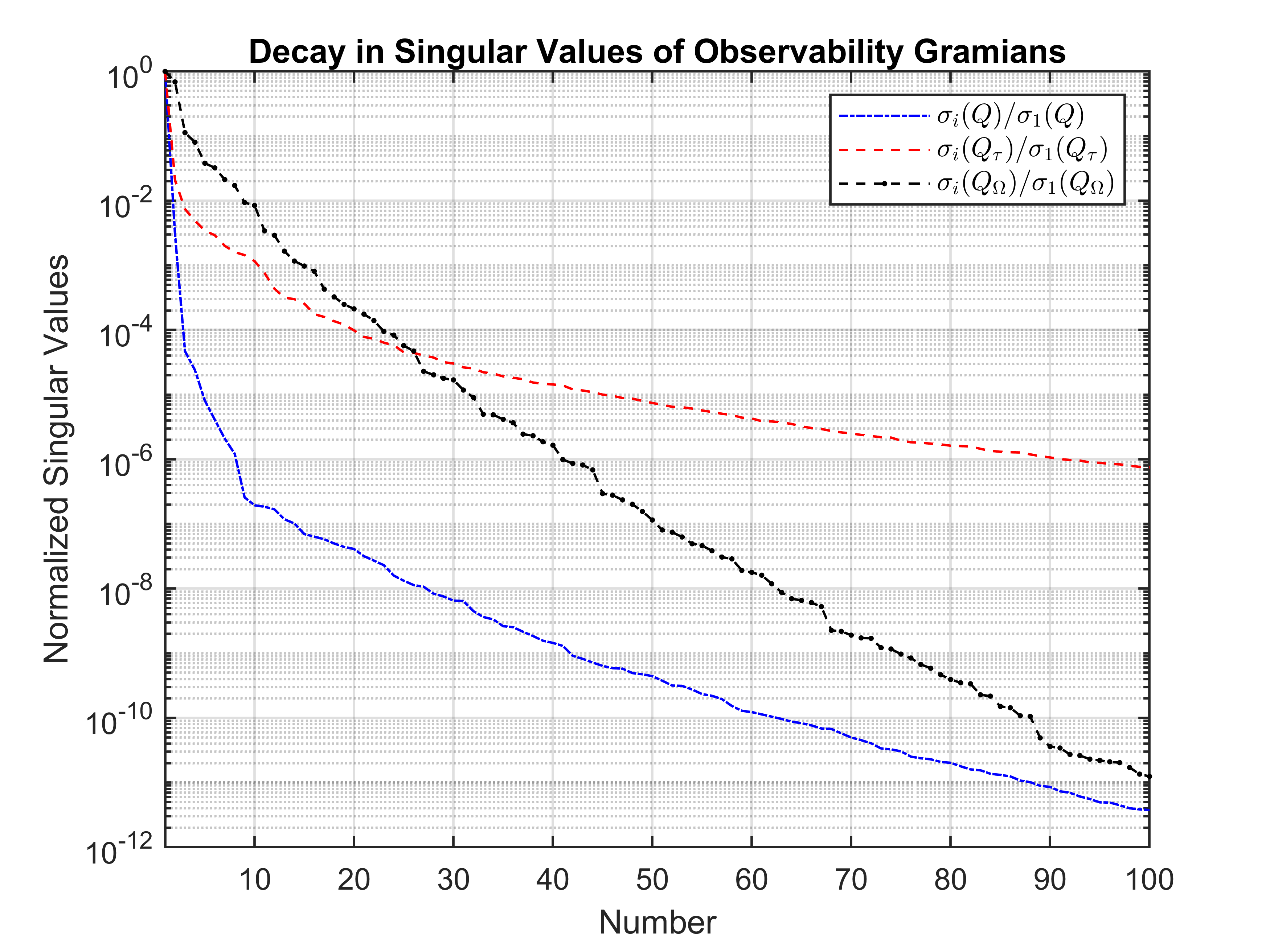
Figure 2: Decay in singular values of $Q$, $Q_{\tau}$, and $Q_{\Omega}$

For clarity, only the largest $100$ singular values are displayed in Figures 1 and 2. It is evident that the decay of all Gramians’ singular values is very rapid, indicating that these matrices can be effectively replaced with their low-rank approximations without significant loss in accuracy. Notably, the singular values of $P_{\tau}$ and $P_{\Omega}$ decay faster than those of $P$, a trend consistent with findings in [31] and [38]. However, in contrast to expectations based on the standard LTI case, Figure 2 reveals that the singular values of $Q_{\tau}$ and $Q_{\Omega}$ decay slower than those of $Q$ in the LTI-QO case.

We construct $15^{th}$ order ROMs of the clamped beam model with a quadratic output using BT, TLBT, and FLBT. The chosen time and frequency intervals for TLBT and FLBT are $[0,1]$ sec and $[14,16]$ rad/sec, respectively. Figure 3 displays the relative error in output responses to the input $0.01\cos(15t)$ within the specified time interval $[0,1]$.

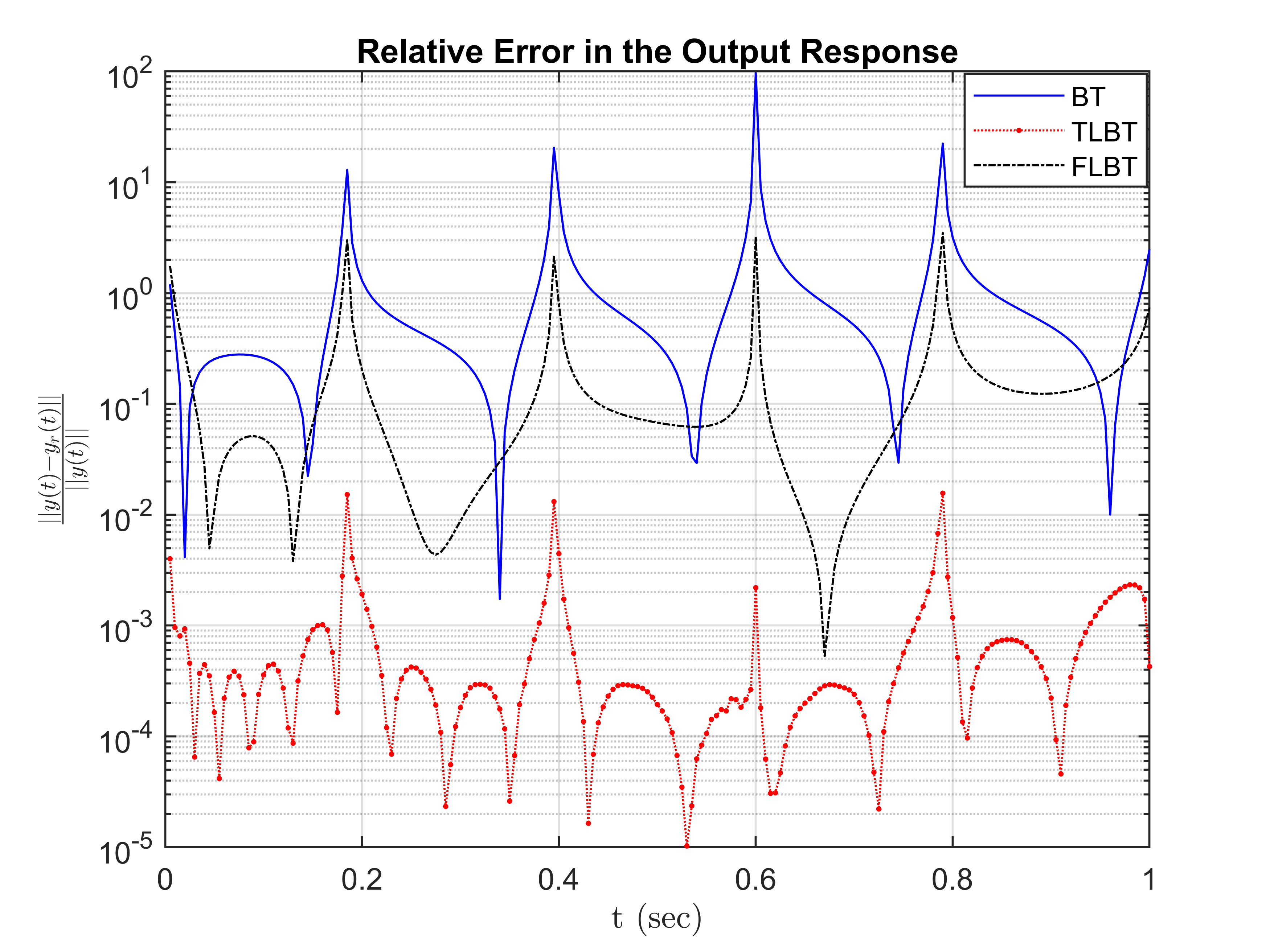
Figure 3: Relative Error in the Output Response within $[0,1]$ sec

As expected, TLBT achieves the highest accuracy within the desired time frame. Additionally, since the input signal’s frequency (15 rad/sec) falls within FLBT’s desired frequency interval, FLBT also yields superior accuracy compared to BT.

6.2 Flexible Space Structure

The flexible space structure benchmark is a procedural modal model that simulates structural dynamics with customizable numbers of actuators and sensors [60]. This model serves as a representation of truss structures in space environments, such as the COFS-1 (Control of Flexible Structures) mass flight experiment. MATLAB code for generating various flexible space structures by specifying the number of actuators and sensors is available in the MORwiki database of benchmark examples [60].

In this example, we generated a $5000^{th}$ order standard state-space model using the MATLAB code provided in MORwiki [60], specifying $2500$ modes, $1$ input actuator, and $1$ output actuator. Subsequently, we introduced a quadratic term $x(t)^{T}Mx(t)$ to the model’s output, where $M\in\mathbb{R}^{5000\times 5000}$ is a diagonal matrix, and $x(t)^{T}Mx(t)$ represents the sum of $200$ randomly selected states. The selection of these states was performed by setting $200$ randomly chosen elements of $M$ to $1$ using MATLAB’s command “randperm(5000,200)”.

Next, we constructed $35^{th}$ order ROMs of this flexible space structure with a quadratic output using BT, TLBT, and FLBT. For TLBT and FLBT, we specified the desired time and frequency intervals as $[0,2]$ sec and $[30,32]$ rad/sec, respectively. Figure 4 presents the relative error in the output responses to the input $0.01\cos(31t)$ within the specified time interval $[0,2]$. Notably, TLBT achieved the highest accuracy for the most part within the desired time interval, except for a few spikes in the relative error. Similarly, FLBT also demonstrated better accuracy than BT (except for a few spikes in the relative error), as the input signal’s frequency ($31$ rad/sec) falls within the desired frequency interval.

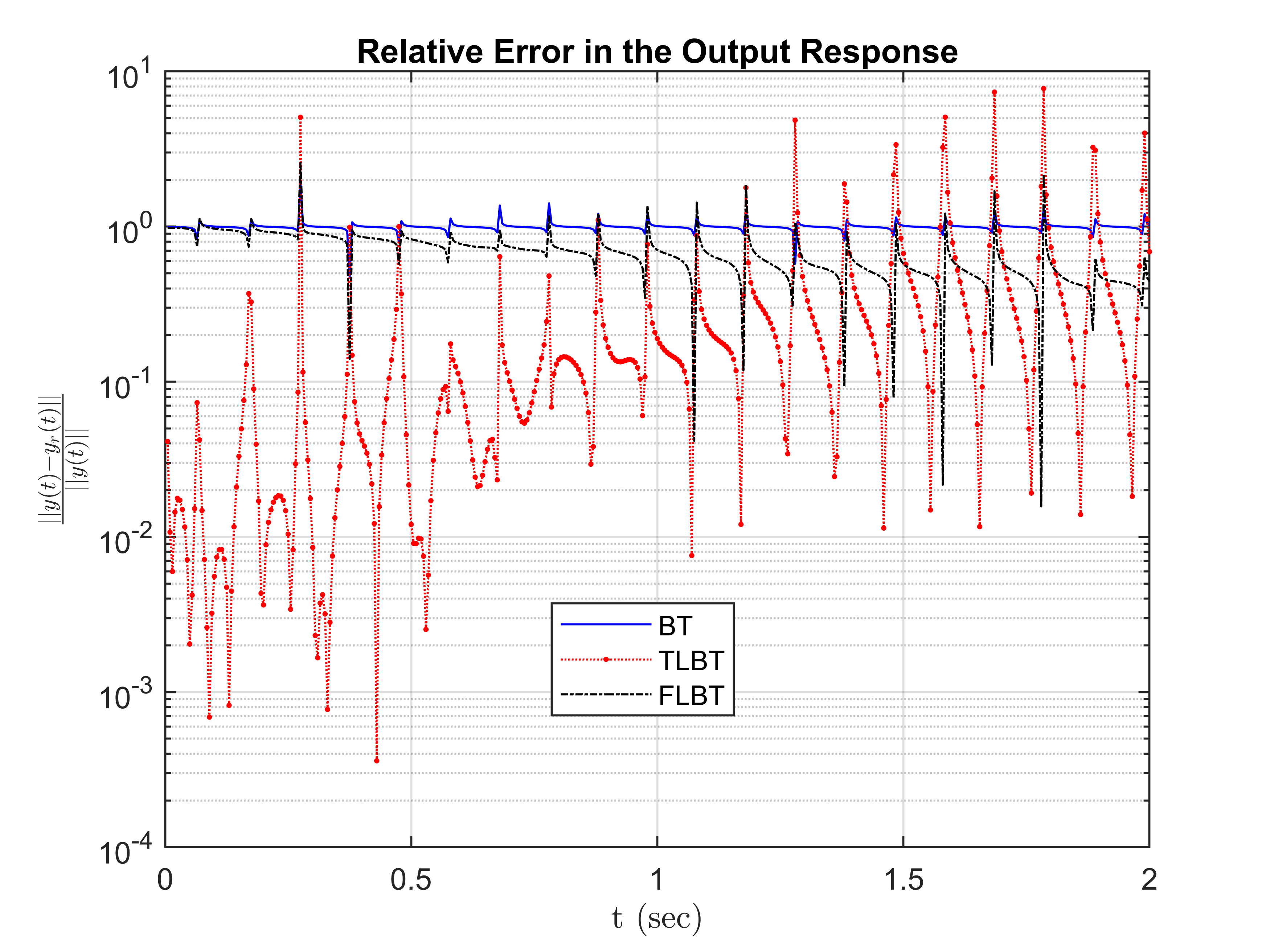
Figure 4: Relative Error in the Output Response within $[0,2]$ sec

7 Conclusion

This paper investigates MOR of LTI-QO systems, focusing on time-limited and frequency-limited scenarios. The recently introduced BT algorithm [1] is extended to address time-limited and frequency-limited cases. Definitions for time-limited and frequency-limited controllability and observability Gramians are given, establishing them as solutions to specific Lyapunov equations. Additionally, low-rank solutions for these Lyapunov equations are discussed. Specifically, the Laguerre expansion-based approach, used to obtain low-rank Cholesky factors for system Gramians, is adapted for computing low-rank Cholesky factors of time-limited and frequency-limited Gramians for LTI-QO systems. The paper also sheds light on potential weaknesses in the Laguerre expansion-based approach. A numerical experiment examines the decay in singular values of time-limited and frequency-limited Gramians. The efficacy of the proposed TLBT and FLBT algorithms is demonstrated through the reduction of two benchmark dynamical systems. The results affirm that the proposed algorithms ensure superior accuracy within the specified time and frequency intervals compared to the BT algorithm.

References

- [1] P. Benner, P. Goyal, I. P. Duff, Gramians, energy functionals, and balanced truncation for linear dynamical systems with quadratic outputs, IEEE Transactions on Automatic Control 67 (2) (2021) 886–893.
- [2] P. Benner, M. Hinze, E. J. W. Ter Maten, Model reduction for circuit simulation, Vol. 74, Springer, 2011.
- [3] W. H. Schilders, H. A. Van der Vorst, J. Rommes, Model order reduction: theory, research aspects and applications, Vol. 13, Springer, 2008.
- [4] A. C. Antoulas, Approximation of large-scale dynamical systems, SIAM, 2005.
- [5] G. Obinata, B. D. Anderson, Model reduction for control system design, Springer Science & Business Media, 2012.
- [6] B. Moore, Principal component analysis in linear systems: Controllability, observability, and model reduction, IEEE transactions on automatic control 26 (1) (1981) 17–32.
- [7] D. F. Enns, Model reduction with balanced realizations: An error bound and a frequency weighted generalization, in: The 23rd IEEE conference on decision and control, IEEE, 1984, pp. 127–132.
- [8] V. Mehrmann, T. Stykel, Balanced truncation model reduction for large-scale systems in descriptor form, in: Dimension Reduction of Large-Scale Systems: Proceedings of a Workshop held in Oberwolfach, Germany, October 19–25, 2003, Springer, 2005, pp. 83–115.
- [9] M. Heinkenschloss, D. C. Sorensen, K. Sun, Balanced truncation model reduction for a class of descriptor systems with application to the oseen equations, SIAM Journal on Scientific Computing 30 (2) (2008) 1038–1063.
- [10] Y. Chahlaoui, D. Lemonnier, A. Vandendorpe, P. Van Dooren, Second-order balanced truncation, Linear algebra and its applications 415 (2-3) (2006) 373–384.
- [11] T. Reis, T. Stykel, Balanced truncation model reduction of second-order systems, Mathematical and Computer Modelling of Dynamical Systems 14 (5) (2008) 391–406.
- [12] H. Sandberg, A. Rantzer, Balanced truncation of linear time-varying systems, IEEE Transactions on automatic control 49 (2) (2004) 217–229.
- [13] S. Lall, C. Beck, Error-bounds for balanced model-reduction of linear time-varying systems, IEEE Transactions on Automatic Control 48 (6) (2003) 946–956.
- [14] P. Benner, S. Gugercin, K. Willcox, A survey of projection-based model reduction methods for parametric dynamical systems, SIAM review 57 (4) (2015) 483–531.
- [15] N. T. Son, P.-Y. Gousenbourger, E. Massart, T. Stykel, Balanced truncation for parametric linear systems using interpolation of Gramians: a comparison of algebraic and geometric approaches, Model Reduction of Complex Dynamical Systems (2021) 31–51.
- [16] S. Lall, J. E. Marsden, S. Glavaški, A subspace approach to balanced truncation for model reduction of nonlinear control systems, International Journal of Robust and Nonlinear Control: IFAC-Affiliated Journal 12 (6) (2002) 519–535.
- [17] S. Lall, J. E. Marsden, S. Glavaški, Empirical model reduction of controlled nonlinear systems, IFAC Proceedings Volumes 32 (2) (1999) 2598–2603.
- [18] B. Kramer, K. Willcox, Balanced truncation model reduction for lifted nonlinear systems, in: Realization and Model Reduction of Dynamical Systems: A Festschrift in Honor of the 70th Birthday of Thanos Antoulas, Springer, 2022, pp. 157–174.
- [19] L. Zhang, J. Lam, B. Huang, G.-H. Yang, On Gramians and balanced truncation of discrete-time bilinear systems, International Journal of Control 76 (4) (2003) 414–427.
- [20] I. P. Duff, P. Goyal, P. Benner, Balanced truncation for a special class of bilinear descriptor systems, IEEE Control Systems Letters 3 (3) (2019) 535–540.
- [21] T. Reis, T. Stykel, Positive real and bounded real balancing for model reduction of descriptor systems, International Journal of Control 83 (1) (2010) 74–88.
- [22] P. C. Opdenacker, E. A. Jonckheere, A contraction mapping preserving balanced reduction scheme and its infinity norm error bounds, IEEE Transactions on Circuits and Systems 35 (2) (1988) 184–189.
- [23] J. Phillips, L. Daniel, L. M. Silveira, Guaranteed passive balancing transformations for model order reduction, in: Proceedings of the 39th Annual Design Automation Conference, 2002, pp. 52–57.
- [24] A. Sarkar, J. M. Scherpen, Structure-preserving generalized balanced truncation for nonlinear port-hamiltonian systems, Systems & Control Letters 174 (2023) 105501.
- [25] P. Borja, J. M. Scherpen, K. Fujimoto, Extended balancing of continuous lti systems: a structure-preserving approach, IEEE Transactions on Automatic Control (2021).
- [26] S. Gugercin, A. C. Antoulas, A survey of model reduction by balanced truncation and some new results, International Journal of Control 77 (8) (2004) 748–766.
- [27] P. Kundur, Power system stability, Power system stability and control 10 (2007) 7–1.
- [28] P. W. Sauer, M. A. Pai, J. H. Chow, Power system dynamics and stability: with synchrophasor measurement and power system toolbox, John Wiley & Sons, 2017.
- [29] M. Grimble, Solution of finite-time optimal control problems with mixed end constraints in the s-domain, IEEE Transactions on Automatic Control 24 (1) (1979) 100–108.
- [30] W. Gawronski, J.-N. Juang, Model reduction in limited time and frequency intervals, International Journal of Systems Science 21 (2) (1990) 349–376.
- [31] P. Kürschner, Balanced truncation model order reduction in limited time intervals for large systems, Advances in Computational Mathematics 44 (6) (2018) 1821–1844.
- [32] K. S. Haider, A. Ghafoor, M. Imran, F. M. Malik, Model reduction of large scale descriptor systems using time limited Gramians, Asian Journal of Control 19 (3) (2017) 1217–1227.
- [33] P. Benner, S. W. Werner, Frequency-and time-limited balanced truncation for large-scale second-order systems, Linear Algebra and its Applications 623 (2021) 68–103.
- [34] H. R. Shaker, M. Tahavori, Time-interval model reduction of bilinear systems, International Journal of Control 87 (8) (2014) 1487–1495.
- [35] A. Jazlan, U. Zulfiqar, V. Sreeram, D. Kumar, R. Togneri, H. F. M. Zaki, Frequency interval model reduction of complex fir digital filters, Numerical Algebra, Control & Optimization 9 (3) (2019) 319–326.
- [36] P. Wortelbore, Frequency weighted balanced reduction of closed-loop mechanical servo-systems: theory and tools, Ph. D. thesis, Delft University of Technology (1994).
- [37] U. Zulfiqar, V. Sreeram, X. Du, Finite-frequency power system reduction, International Journal of Electrical Power & Energy Systems 113 (2019) 35–44.
- [38] P. Benner, P. Kürschner, J. Saak, Frequency-limited balanced truncation with low-rank approximations, SIAM Journal on Scientific Computing 38 (1) (2016) A471–A499.
- [39] M. Imran, A. Ghafoor, Model reduction of descriptor systems using frequency limited Gramians, Journal of the Franklin Institute 352 (1) (2015) 33–51.
- [40] H. R. Shaker, M. Tahavori, Frequency-interval model reduction of bilinear systems, IEEE Transactions on Automatic Control 59 (7) (2013) 1948–1953.
- [41] C. A. Depken, The observability of systems with linear dynamics and quadratic output., Ph.D. thesis, Georgia Institute of Technology (1974).
- [42] B. Haasdonk, K. Urban, B. Wieland, Reduced basis methods for parameterized partial differential equations with stochastic influences using the Karhunen–Loève expansion, SIAM/ASA Journal on Uncertainty Quantification 1 (1) (2013) 79–105.
- [43] L. D. Lutes, S. Sarkani, Random vibrations: analysis of structural and mechanical systems, Butterworth-Heinemann, 2004.
- [44] M. Hammerschmidt, S. Herrmann, J. Pomplun, L. Zschiedrich, S. Burger, F. Schmidt, Reduced basis method for maxwell’s equations with resonance phenomena, in: Optical Systems Design 2015: Computational Optics, Vol. 9630, SPIE, 2015, pp. 138–151.
- [45] M. W. Hess, P. Benner, Output error estimates in reduced basis methods for time-harmonic maxwell’s equations, in: Numerical Mathematics and Advanced Applications ENUMATH 2015, Springer, 2016, pp. 351–358.
- [46] R. Van Beeumen, K. Meerbergen, Model reduction by balanced truncation of linear systems with a quadratic output, in: AIP Conference Proceedings, Vol. 1281, American Institute of Physics, 2010, pp. 2033–2036.
- [47] R. Pulch, A. Narayan, Balanced truncation for model order reduction of linear dynamical systems with quadratic outputs, SIAM Journal on Scientific Computing 41 (4) (2019) A2270–A2295.
- [48] M. I. Ahmad, I. Jaimoukha, M. Frangos, Krylov subspace restart scheme for solving large-scale Sylvester equations, in: Proceedings of the 2010 American control conference, IEEE, 2010, pp. 5726–5731.
- [49] P. Benner, P. Kürschner, J. Saak, Self-generating and efficient shift parameters in ADI methods for large Lyapunov and Sylvester equations, Electronic Transactions on Numerical Analysis 43 (2014) 142–162.
- [50] P. Benner, J. Saak, Numerical solution of large and sparse continuous time algebraic matrix Riccati and Lyapunov equations: a state of the art survey, GAMM-Mitteilungen 36 (1) (2013) 32–52.
- [51] N. Lang, H. Mena, J. Saak, An factorization based ADI algorithm for solving large-scale differential matrix equations, PAMM 14 (1) (2014) 827–828.
- [52] Z.-H. Xiao, Q.-Y. Song, Y.-L. Jiang, Z.-Z. Qi, Model order reduction of linear and bilinear systems via low-rank Gramian approximation, Applied Mathematical Modelling 106 (2022) 100–113.
- [53] J.-R. Li, J. White, Low rank solution of Lyapunov equations, SIAM Journal on Matrix Analysis and Applications 24 (1) (2002) 260–280.
- [54] R. Eid, Time domain model reduction by moment matching, Ph.D. thesis, Technische Universität München (2009).
- [55] T. Wolf, H. K. Panzer, The ADI iteration for Lyapunov equations implicitly performs pseudo-optimal model order reduction, International Journal of Control 89 (3) (2016) 481–493.
- [56] M. S. Tombs, I. Postlethwaite, Truncated balanced realization of a stable non-minimal state-space system, International Journal of Control 46 (4) (1987) 1319–1330.
- [57] D. Petersson, J. Löfberg, Model reduction using a frequency-limited -cost, Systems & Control Letters 67 (2014) 32–39.
- [58] D. Petersson, A nonlinear optimization approach to -optimal modeling and control, Ph.D. thesis, Linköping University Electronic Press (2013).
- [59] Y. Chahlaoui, P. Van Dooren, Benchmark examples for model reduction of linear time-invariant dynamical systems, in: Dimension Reduction of Large-Scale Systems: Proceedings of a Workshop held in Oberwolfach, Germany, October 19–25, 2003, Springer, 2005, pp. 379–392.
- [60] P. Benner, K. Lund, J. Saak, Towards a benchmark framework for model order reduction in the mathematical research data initiative (MARDI), PAMM 23 (3) (2023) e202300147.
- [61] P. Benner, S. W. Werner, MORLAB–the model order reduction laboratory, Model Reduction of Complex Dynamical Systems (2021) 393–415.