The Assignment Game: New Mechanisms
for Equitable Core Imputations

Abstract

The set of core imputations of the assignment game forms a (non-finite) distributive lattice. So far, efficient algorithms were known for computing only its two extreme imputations; however, each of them maximally favors one side and disfavors the other side of the bipartition, leading to inequitable profit sharing. Another issue is that a sub-coalition consisting of one player (or a set of players from the same side of the bipartition) can make zero profit, therefore a core imputation is not obliged to give them any profit. Hence core imputations make no fairness guarantee at the level of individual agents. This raises the question of computing more equitable core imputations.

In this paper, we give combinatorial (i.e., the mechanism does not invoke an LP-solver) polynomial time mechanisms for computing the leximin and leximax core imputations for the assignment game. These imputations achieve “fairness” in different ways: whereas leximin tries to make poor agents more rich, leximax tries to make rich agents less rich. In general, the two imputations are different.

Our mechanisms were derived by a suitable adaptation of the classical primal-dual paradigm from combinatorial optimization. The “engine” driving them involves recent insights, obtained via complementarity, into core imputations [Vaz22] and the pristine combinatorial structure of matching. We have identified other natural games which could benefit from our approach.

1 Introduction

Equality and fair division are timeless values which have taken centerstage in economics all the way from the early days of social choice theory [Arr12] to the Internet age [Mou19]. Within cooperative game theory, the core is considered the gold standard solution concept for “fair” profit sharing. It distributes the total worth of a game among the agents in such a way that the total profit received by a sub-coalition is commensurate with its inherent worth, the latter being the profit which the sub-coalition can generate all by itself. Thus a core imputation is fair to each of exponentially many sub-coalitions – a stringent requirement indeed. However, as we will see in the context of the assignment game, not all core imputations are equally fair and it is possible to optimize among the core imputations. We will give polynomial time mechanisms for computing two special core imputations for this game.

The assignment game forms a paradigmatic setting for studying the notion of core of a transferable utility (TU) market game, in large part because of the work of Shapley and Shubik [SS71]. They characterized the core of the assignment game: they showed that the set of its core imputations is precisely the set of optimal solutions to the dual of the LP-relaxation of the maximum weight matching problem in the underlying bipartite graph; the weight of this matching is the worth of the game. The assignment game is widely applicable, e.g., Shapley and Shubik present it in the context of the housing market game in which the two sides of the bipartition are buyers and sellers of houses.

Shapley and Shubik also proved that the set of core imputations of the assignment game forms a lattice. The top and bottom elements of this lattice form two extreme imputations, each maximally favoring one side and disfavoring the other side of the bipartition. So far efficient algorithms were known for computing only these two extreme imputations, which in a sense are the least fair among core imputations, see Section 3.1. Their convex combination is also a core imputation; however, it is not clear what fairness properties it possesses.

Another issue is that a sub-coalition consisting of one player (or a set of players from the same side of the bipartition) can make zero profit, therefore a core imputation is not obliged to give them any profit. Hence core imputations make no fairness guarantee at the level of individual agents. This fact was first observed in a prominent work by Dutta and Ray [DR89]. They proceeded to find a middle-ground in the tension between sub-coalitions demanding profit which is commensurate with their inherent worth and the societal norm of “equality” as a desirable outcome by showing that a convex game admits a unique core imputation which Lorenz dominates all other core imputations; they call it the egalitarian solution.

From our standpoint, this work has three shortcomings: it does not apply to the assignment game, it is not efficiently computable for any non-trivial, natural game, and the Lorenz order is partial and not a total order. Our work address all three issues. As shown by Shapley and Shubik, the set of core imputations of the assignment game is the entire polytope of optimal dual solutions, i.e., in general it is a dense set consisting of uncountably many elements. Are there special elements in this set which are equitable to both sides and to individual agents?

At this point, a useful perspective is provided by a similar situation that arises in the stable matching game of Gale and Shapley [GS62], which is a non-transferable utility (NTU) game. The core of this game is the set of all stable matchings — each ensures that no coalition formed by one agent from each side of the bipartition has an incentive to secede. It is well known that this set forms a finite distributive lattice whose top and bottom elements maximally favor one side and disfavor the other side of the bipartition. Furthermore, the deferred acceptance algorithm of Gale and Shapley can find only these two extreme matchings.

Since several applications of this game call for stable matchings which are more equitable to both sides, the question of finding such matchings efficiently has garnered much attention, leading to efficient algorithms as well as intractability results, see [ILG87, TS98, Che10, CMS11, EIV23]. The efficient algorithms crucially use Birkhoff’s Representation Theorem for finite distributive lattices [Bir37] and the notion of rotations [IL86].

We note that although the lattice of core imputations of an assignment game is distributive, it is not finite and therefore Birkhoff’s Representation Theorem does not apply to it. Hence new ideas are required for answering the question stated above. In this context we ask: What are desirable properties for a core imputation to be called equitable? A reasonable answer appears to be: the imputation should be either leximin or leximax among all core imputations.

In this paper we give combinatorial polynomial time mechanisms for computing such imputations for the assignment game. These two imputations achieve equality in different ways: whereas leximin tries to make poor agents more rich, leximax tries to make rich agents less rich. In general, the two imputations are different and a deeper study of their pros and cons is called for. Properties of their convex combinations are also worth exploring.

Our mechanisms were derived by a suitable adaptation of the classical primal-dual paradigm from combinatorial optimization, see Section 5.1. The “engine” driving them involves insights, obtained via complementarity, into core imputations, see Section 3.2. Observe that the worth of the assignment game is given by an optimal solution to the primal LP and its core imputations are given by optimal solutions to the dual LP. Although it is well known that the fundamental fact connecting these two solutions is complementary slackness conditions, somehow the implications of this fact were explored only recently, in [Vaz22], over half a century after [SS71].

Our mechanisms were also beneficiaries of the pristine combinatorial structure of matching. Within the area of algorithm design, the “right” technique for solving several types of algorithmic questions was first discovered in the context of matching and later these insights were applied to other problems. We expect a similar phenomenon here. In this context, it will be interesting to seek leximin and leximax core imputations for the flow game of Kalai and Zemel [KZ82] as well as the minimum cost spanning tree game. For the latter game, Granot and Huberman [GH81, GH84] showed that the core is non-empty and gave an algorithm for finding an imputation in it.

2 Related Works

In a prominent work, Dutta and Ray [DR89] attempt to find a middle-ground in the tension between sub-coalitions demanding profit which is commensurate with their inherent worth and the societal norm of “equality” as a desirable outcome. They show that a convex game admits a unique core imputation which Lorenz dominates all other core imputations; they call it the egalitarian solution. From our standpoint, this work has two shortcomings: it does not apply to the assignment game and it is not efficiently computable for any non-trivial, natural game. Our work address both these issues. Another difference is that whereas the Lorenz order is partial, leximin and leximax are total orders.

The importance of “fair” profit-sharing has been recognized for the proper functioning of all aspects of society — from personal relationships to business collaborations. Moreover, this has been a consideration since ancient times, e.g., see the delightful and thought-provoking paper by Aumann and Maschler [AM85], which discusses problems from the 2000-year-old Babylonian Talmud on how to divide the estate of a dead man among his creditors.

Below we state results giving LP-based core imputations for natural games; these are also candidates for the study of leximin and leximax core imputations. Deng et al. [DIN99] gave LP-based characterization of the cores of several combinatorial optimization games, including maximum flow in unit capacity networks both directed and undirected, maximum number of edge-disjoint $s$-$t$ paths, maximum number of vertex-disjoint $s$-$t$ paths, maximum number of disjoint arborescences rooted at a vertex $r$, and general graph matching game in which the weight of optimal fractional and integral matchings are equal (such a game has a non-empty core).

In a different direction, Vande Vate [Vat89] and Rothblum [Rot92] gave linear programming formulations for stable matchings; the vertices of their underlying polytopes are integral and are stable matchings. More recently, Kiraly and Pap [KP08] showed that the linear system of Rothblum is in fact totally dual integral (TDI).

Koh and Sanita [KS20] answer the question of efficiently determining if a spanning tree game is submodular; the core of such games is always non-empty. Nagamochi et al. [NZKI97] characterize non-emptyness of core for the minimum base game in a matroid; the minimum spanning tree game is a special case of this game. Lastly, [Vaz22] gives an LP-based characterization for the core of the $b$-matching game.

3 Definitions and Preliminary Facts

After giving some basic definitions, we will state Shapley and Shubik’s results for the assignment game as well as insights obtained in [Vaz22] via complementarity. For an extensive coverage of cooperative game theory, see the book by Moulin [Mou14].

Definition 1.

In a transferable utility (TU) market game, utilities of the agents are stated in monetary terms and side payments are allowed.

Definition 2.

A cooperative game consists of a pair $(N,c)$ where $N$ is a set of $n$ agents and $c$ is the characteristic function; $c:2^{N}\rightarrow\mathcal{Q}_{+}$, where for $S\subseteq N,\ c(S)$ is the worth that the sub-coalition $S$ can generate by itself. $N$ is also called the grand coalition.

Definition 3.

An imputation is a function $p:N\rightarrow\mathcal{Q}_{+}$ that gives a way of dividing the worth of the game, $c(N)$, among the agents. It satisfies $\sum_{i\in N}{p(i)}=c(N)$; $p(i)$ is called the profit of agent $i$.

Definition 4.

An imputation $p$ is said to be in the core of the game $(N,c)$ if for any sub-coalition $S\subseteq N$, the total profit allocated to agents in $S$ is at least as large as the worth that they can generate by themselves, i.e., $\sum_{i\in S}{p(i)}\geq c(S)$.

3.1 The Results of Shapley and Shubik for the Assignment Game

The assignment game consists of a bipartite graph $G=(U,V,E)$ and a weight function for the edges $w:E\rightarrow\mathcal{Q}_{+}$, where we assume that each edge has positive weight; otherwise the edge can be removed from $G$. The agents of the game are the vertices, $U\cup V$ and the total worth of the game is the weight of a maximum weight matching in $G$; the latter needs to be distributed among the vertices.

For this game, a sub-coalition $(U^{\prime}\cup V^{\prime})$ consists of a subset of the agents, also called vertices, with $U^{\prime}\subseteq U$ and $V^{\prime}\subseteq V$. The worth of a sub-coalition $(U^{\prime}\cup V^{\prime})$ is defined to be the weight of a maximum weight matching in the graph $G$ restricted to vertices in $(U^{\prime}\cup V^{\prime})$ and is denoted by $c(U^{\prime}\cup V^{\prime})$. The characteristic function of the game is defined to be $c:2^{U\cup V}\rightarrow\mathcal{Q}_{+}$.

An imputation consists of two functions $u:{U}\rightarrow\mathcal{Q}_{+}$ and $v:{V}\rightarrow\mathcal{Q}_{+}$ such that $\sum_{i\in U}{u_{i}}+\sum_{j\in V}{v_{j}}=c(U\cup V)$. Imputation $(u,v)$ is said to be in the core of the assignment game if for any sub-coalition $(U^{\prime}\cup V^{\prime})$, the total profit allocated to agents in the sub-coalition is at least as large as the worth that they can generate by themselves, i.e., $\sum_{i\in U^{\prime}}{u_{i}}+\sum_{j\in V^{\prime}}{v_{j}}\geq c(S)$.

Linear program (3.1) gives the LP-relaxation of the problem of finding a maximum weight matching in $G$. In this program, variable $x_{ij}$ indicates the extent to which edge $(i,j)$ is picked in the solution. ∑_(i, j) ∈E w_ij x_ij ∑_(i, j) ∈E x_ij≤1  ∀i ∈U ∑_(i, j) ∈E x_ij≤1 ∀j ∈V x_ij≥0∀(i, j) ∈E Taking $u_{i}$ and $v_{j}$ to be the dual variables for the first and second constraints of (3.1), we obtain the dual LP: ∑_i ∈U u_i + ∑_j ∈V v_j u_i + v_j ≥w_ij  ∀(i, j) ∈E u_i≥0∀i ∈U v_j≥0∀j ∈V The constraint matrix of LP (3.1) is totally unimodular and therefore the polytope defined by its constraints is integral; its vertices are matchings in the underlying graph.

Theorem 1.

(Shapley and Shubik [SS71]) The dual LP, (3.1) completely characterizes the core of the assignment game.

By this theorem, the core is a convex polyhedron. Shapley and Shubik further showed that the set $S$ of core imputations of the assignment game forms a lattice under the following partial order on $S$: Given two core imputations $(u,v)$ and $(u^{\prime},v^{\prime})$, say that $(u,v)\leq(u^{\prime},v^{\prime})$ if for each $i\in U$, $u_{i}\geq u_{i}^{\prime}$; if so, it must be that for each $j\in V,v_{j}\leq v_{j}^{\prime}$. This partial order supports meet and join operations: given two core imputations $(u,v)$ and $(u^{\prime},v^{\prime})$, for each $i\in U$, the meet chooses the bigger of $u_{i}$ and $u_{i}^{\prime}$ and the join chooses the smaller. It is easy to see that the lattice is distributive.

Define $u^{h}$ and $u^{l}$ as follows: For $i\in U$, let $u_{i}^{h}$ and $u_{i}^{l}$ denote the highest and lowest profits that $i$ accrues among all imputations in the core. Similarly, define $v^{h}$ and $v^{l}$.

Theorem 2.

(Shapley and Shubik [SS71]) Under the partial order defined above, the core of the assignment game forms a distributive lattice; its two extreme imputations are $(u^{h},v^{l})$ and $(u^{l},v^{h})$.

Definition 5.

We will say that the two extreme imputations, $(u^{h},v^{l})$ and $(u^{l},v^{h})$, are the $U$-optimal and $V$-optimal core imputations, respectively.

The two extreme imputations can be efficiently obtained as follows. First find a maximum weight matching in $G$; a fractional one found by solving LP (3.1) will suffice. Let its picked edges be $M\subseteq E$. The $U$-optimal core imputation is obtained by solving LP (5) and the $V$-optimal imputation can be similarly obtained.

∑_i ∈U u_i u_i + v_j = w_ij  ∀(i, j) ∈M u_i + v_j ≥w_ij  ∀(i, j) ∈E u_i≥0∀i ∈U v_j≥0∀j ∈V

3.2 Insights Obtained via Complementarity

Definition 6.

A generic vertex/agent in $U\cup V$ will be denoted by $q$. We will say that $q$ is:

1. essential if $q$ is matched in every maximum weight matching in $G$.

2. viable if there is a maximum weight matching $M$ such that $q$ is matched in $M$ and another, $M^{\prime}$ such that $q$ is not matched in $M^{\prime}$.

3. subpar if for every maximum weight matching $M$ in $G$, $q$ is not matched in $M$.

Definition 7.

Let $y$ be an imputation in the core. We will say that $q$ gets paid in $y$ if $y_{q}>0$ and does not get paid otherwise. Furthermore, $q$ is paid sometimes if there is at least one imputation in the core under which $q$ gets paid, and it is never paid if it is not paid under every imputation.

Theorem 3.

(Vazirani [Vaz22]) For every vertex $q\in(U\cup V)$:

$$q\ \mbox{is paid sometimes}\ \iff\ q\ \mbox{is essential}$$

Thus core imputations pay only essential vertices and each of them is paid in some core imputation.

Definition 8.

We will say that an edge $(i,j)$ is tight if $u_{i}+v_{j}=w_{ij}$, it is over-tight if $u_{i}+v_{j}>w_{ij}$ and it is under-tight if $u_{i}+v_{j}<w_{ij}$.

Definition 9.

We will say that $e=(i,j)$ is:

1. essential if $e$ is matched in every maximum weight matching in $G$.

2. viable if there is a maximum weight matching $M$ such that $e\in M$, and another, $M^{\prime}$ such that $e\notin M^{\prime}$.

3. subpar if for every maximum weight matching $M$ in $G$, $e\notin M$.

Theorem 4.

(Vazirani [Vaz22]) For every edge $e\in E$:

$$e\ \mbox{is always tight}\ \iff\ e\ \mbox{is viable or essential}$$

By the constraint in LP (3.1), in any feasible dual, no edge is under-tight. By Theorem 4, every subpar edge is over-tight in some optimal dual.

Definition 10.

An assignment game is said to be non-degenerate if it has a unique maximum weight matching.

In a non-degenerate assignment game there are no viable vertices or edges, i.e., every vertex and edge is either essential or subpar.

3.3 Efficient Procedures for Classifying Vertices and Edges

In this section, we will give polynomial time procedures for partitioning vertices and edges according to the classification given in Definitions 6 and 9. This is required by the mechanisms given in Sections 6 and 7.

Let $W_{\max}$ be the worth of the given assignment game, $G=(U,V,E),\ w:E\rightarrow\mathcal{Q}_{+}$. For each edge $e$, find the worth of the game with $e$ removed. If it is less than $W_{max}$ then $e$ is essential. Now pick an edge $e^{\prime}$ which is not essential and let its weight be $w$. Remove the two endpoints of $e^{\prime}$ and compute the worth of the remaining game. If it is $(W_{\max}-w)$, then $e^{\prime}$ is viable, since it is not essential and is matched in a maximum weight matching. The remaining edges are subpar.

Next, for each vertex $v$, consider the game with player $v$ removed and find its worth. If it is less than $W_{max}$ then $v$ is essential. The endpoints of all viable edges are either essential or viable. Therefore, dropping the essential vertices from these yield viable vertices. Finally, a vertex which does not have an essential or viable edge incident at it is subpar.

4 Leximin and Leximax Core Imputations

In this section, we will define leximin and leximax core imputations for the assignment game, show why each is unique and give an example in which they are different, see Example 1. Note that in all examples given in this paper, essential and viable edges are represent by solid lines and subpar edges by dotted lines.

Let $U_{e}\subseteq U$ and $V_{e}\subseteq V$ be the sets of essential players in the assignment game, $G=(U,V,E),\ w:E\rightarrow\mathcal{Q}_{+}$. As stated in Theorem 3, every core imputation allocates the entire profit to players in $U_{e}\cup V_{e}$ only.

Definition 11.

For each core imputation of the assignment game $G=(U,V,E),\ w:E\rightarrow\mathcal{Q}_{+}$, sort the allocations made to players $U_{e}\cup V_{e}$ in increasing order. Let $L_{1}$ and $L_{2}$ be two such sorted lists. Then $L_{1}$ is lexicographically larger than $L_{2}$ if in the first index at which the two lists differ, $L_{1}$ has a larger entry than $L_{2}$; note that these two entries may be profits of different players. An imputation yielding the lexicographically largest list will be called a leximin core imputation. Lemma 1 shows that such an imputation is unique.

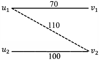
Figure 1: The graph for Example 1

.

Lemma 1.

(Moulin [Mou91]) The set of leximin core imputations for a convex game is a singleton.

The proof of Lemma 1 follows easily via a contradiction: Suppose there are two leximin core imputations, then their average is also a core imputation and will be lexicographically larger than both of them.

Definition 12.

For each core imputation of the assignment game $G=(U,V,E),\ w:E\rightarrow\mathcal{Q}_{+}$, sort the allocations made to players $U_{e}\cup V_{e}$ in decreasing order. Let $L_{1}$ and $L_{2}$ be two such sorted lists. Then $L_{1}$ is lexicographically smaller than $L_{2}$ if in the first index at which the two lists differ, $L_{1}$ has a smaller entry than $L_{2}$. An imputation yielding the lexicographically smallest list will be called a leximax core imputation. By a proof analogous to that of Lemma 1, such an imputation is unique.

Example 1.

In the graph shown in Figure 1, the leximin and leximax core imputations for vertices $(u_{1},u_{2},v_{1},v_{2})$ are $(40,30,30,70)$ and $(55,45,15,55)$, respectively. The corresponding sorted orders are $30,30,40,70$ and $55,55,45,15$.

5 High Level Ideas

In this section, we will give the high level ideas behind our mechanism for computing the leximin core imputation for the assignment game $G=(U,V,E),\ w:E\rightarrow\mathcal{Q}_{+}$; details are provided in Section 6. The ideas for leximax core imputation are analogous and its details are provided in Section 7.

Under every feasible solution to the dual LP (3.1), every edge must be either tight or over-tight. By complementary slackness conditions, stated in Section 3.2, a feasible dual solution is optimal if and only if the following two conditions are satisfied:

1. Every essential and viable edge is tight.

2. Only essential vertices have positive duals.

By Theorem 1, the set of optimal dual solutions is precisely the set of core imputation of the assignment game. Our mechanism starts by computing an arbitrary such imputation, say $(u.v)$. Clearly this can be done by optimally solving LP (3.1). However, since we wish to give an efficient combinatorial mechanism, we will resort to an efficient combinatorial algorithm for computing a maximum weight matching in a bipartite graph; such an algorithm yields an optimal dual as well, e.g., see [LP86]. Our mechanism maintains the two conditions stated above throughout its run, thereby ensuring that it always has a core imputation.

At the start, our mechanism also computes the sets of essential, viable and subpar edges and vertices using the efficient procedures given in Section 3.3. The starting set of tight edges is denoted by $T_{0}$ and it contains all essential and viable edges. The subgraph of $G$ consisting of the edges of $T_{0}$ is called the starting tight subgraph and is denoted by $H_{0}=(V,T_{0})$. If the given game is non-degenerate, at the start of the mechanism each connected component of $H_{0}$ is either an essential edge or a subpar vertex; the latter is called a trivial component. If the given game is degenerate, $H_{0}$ will also contain connected components consisting of two or more viable edges. As the mechanism proceeds, the set of tight edges grows; it is denoted by $T$ and the tight subgraph by $H=(V,T)$.

5.1 The Primal-Dual Framework and Supporting Ideas

Much like a primal-dual algorithm, our mechanism operates by making primal and dual updates. However, there are fundamental differences, which we will describe by comparing our mechanism to a primal-dual algorithm for finding a maximum weight matching in a bipartite graph; for this reason, we call it a primal-dual-type mechanism.

At the outset, the nature of the two tasks is very different. As is well known, for any weight function for the edges, a maximum weight matching appears at a vertex of the bipartite matching polytope, i.e., the polytope defined by the constraints of the primal LP (3.1). Therefore, the solution lies at one of finitely — though exponentially — many points. As shown by Shapley and Shubik [SS71], the set of core imputations of an assignment game forms a polytope which lies within the polyhedron of feasible solutions of the dual LP (3.1). It is therefore a dense set in general, with uncountably many elements. At present we do not know where in this polytope the leximin and leximax core imputations lie, see Section 8.

The primal-dual algorithm for maximum weight matching starts by computing a feasible dual and an infeasible primal. It then iteratively improves the optimality of the dual and the feasibility of the primal, eventually terminating in optimal primal and dual solutions. Its task is considerably simplified by the powerful complementary slackness conditions, which the optimal pair of solutions must satisfy. These conditions transform the problem of finding a globally optimal solution to the easier task of making local improvements. No analogous device is know for our problem.

The purpose of the primal and dual updates in our mechanism is very different. It starts by computing optimal primal and dual solutions to the maximum weight matching problem; the latter is the starting core imputation. A dual update attempts to leximin-improve the core imputation by altering the profits of certain essential vertices. One of the ways this process is blocked is that a subpar edge $e$ goes exactly tight; continuing the process further will make it go under-tight, leading to an infeasible dual. At this point, the primal update adds $e$ to the tight subgraph $H$, and the mechanism appropriately changes the set of essential vertices whose profit is altered in the next dual update.

Obviously what is described above is a mere framework; little reason is given to support the belief that it can be used to find a globally optimal core imputation. Indeed, a bulk of the work is done by the three key ideas presented in Section 5.4, the primary one being the variable $\Omega$, which helps synchronize the various events that happen during the run of the mechanism. Eventually it helps establish the Invariant stated in Section 6.3, which plays a central role in the proof.

5.2 Characterizing Connected Components of $H_{0}$

We will partition the connected components of $H_{0}$ into two sets as defined below.

Definition 13.

A connected component, $C$, of $H_{0}$, is called a unique imputation component if the profit shares of vertices of $C$ remain unchanged over all possible core imputations.

Definition 14.

A connected component, $C$, of $H_{0}$ which is not a unique imputation component is called a fundamental component.

Corollary 1 is the key fact proved in this section; it follows from Lemmas 2 and 3.

Corollary 1.

A component of $H_{0}$ is fundamental if and only if all its vertices are essential.

Fundamental components are the building blocks which our mechanism works with in the following sense: Each such component comes with profit shares of its essential vertices and these get modified in the dual updates; an important restriction is that the two conditions stated above should always be satisfied, therefore ensuring that the dual is always a core imputation. As stated above, this update gets blocked when a subpar edge goes exactly tight. Much of the mechanism is concerned with appropriately dealing with the latter event.

Definition 15.

For any connected component $C$ of the tight subgraph $H$, $U(C)$ and $V(C)$ will denote the vertices of $C$ in $U$ and $V$, respectively. Furthermore, $\mbox{\rm left}(C)$ will denote $U(C)\cap U_{e}$ and $\mbox{\rm right}(C)$ will denote $V(C)\cap V_{e}$.

In case the reader is interested in understanding the mechanisms in a simpler setting, they may skip the rest of this subsection, under the assumption that the given game is non-degenerate and therefore has no viable vertices and edges.

Some remarks are due about Definitions 13 and 14. Clearly, the endpoints of an essential edge are essential vertices. Such an edge has a non-unique imputation, as shown in Lemma 2, and is therefore a fundamental component. Unique imputation components are of two types: a subpar vertex or a component of viable edges. The former is necessarily an isolated vertex in $H_{0}$ and its profit share is zero in all core imputations. Let $C$ be a fundamental component of viable edges. If $|\mbox{\rm left}(C)|\neq|\mbox{\rm right}(C)|$ then it is easy to see that $C$ must have a unique imputation. For instance, the graph of Figure 2 has the unique imputation of $(100,0,0)$ for the vertices $(u_{1},v_{1},v_{2})$; of these three vertices only $u_{1}$ is essential. On the other hand, if $|\mbox{\rm left}(C)|=|\mbox{\rm right}(C)|$, then $C$ may or may not have a unique imputation; for the former, see Example 2 and for the latter, consider a complete bipartite graph with unit weight edges. Observe that all vertices of the latter example are essential; Lemma 3 proves that a component of viable edges is fundamental if and only if all its vertices are essential.

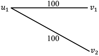
Figure 2: A fundamental component $C$ satisfying $|\mbox{\rm left}(C)|\neq|\mbox{\rm right}(C)|$ and therefore having a unique imputation.

Example 2.

Figure 3 shows a fundamental component $C$ satisfying $|\mbox{\rm left}(C)|=|\mbox{\rm right}(C)|$ and having a unique core imputation; it is $(60,0,0,40)$ for vertices $(u_{1},u_{2},v_{1},v_{2})$.

Lemma 2.

Each essential edge is a fundamental component.

Proof.

For the sake of contradiction, assume that essential edge $(i,j)$ has a unique imputation and let the profit shares of $i$ and $j$ be $a$ and $b$, respectively. Assume w.l.o.g. that $a\geq b$; clearly, $a>0$. If $i$ does not have another edge incident at it in $G$, then changing the profit shares of $i$ and $j$ to $(0,a+b)$ will also lead to a core imputation.

Next assume that $i$ has $k$ other edges incident at it. These $k$ edges must necessarily be subpar and by Theorem 4, each of these edges, there is a core imputation under which the edge is over-tight, to the extent of at least $\epsilon>0$, say. Now the convex combination of these core imputations is also a core imputation in which each of these edges is over-tight to the extent of $\epsilon/k>0$. Therefore, changing the profit shares of $i$ and $j$ to $(a-\epsilon/k,b+\epsilon/k)$ will lead to another core imputation. The contradiction establishes the lemma. ∎

Lemma 3.

Let $C$ be a component of $H_{0}$ consisting of viable edges. Then $C$ is fundamental if and only if all its vertices are essential.

Proof.

First assume that $C$ contains a viable vertex, say $u$. We will use the following two facts, which follow from Theorems 3 and 4, respectively: the profit of all viable vertices is 0 in all core imputations and all edges of $C$ are tight.

We start by observing that we can fix a core imputation under which each essential vertex gets positive profit. We consider two cases: If $C$ has a unique core imputation, this must hold by Theorem 3. Next assume that $C$ admits more than one core imputation. By Theorem 3, corresponding to each essential vertex, there is a core imputation under which it gets positive profit. Then, under the convex combination of these imputations, which is also a core imputation, each essential vertex gets positive profit.

Next, we will show that the profit share of each essential vertex is forced to be unique, thereby proving that the first case must hold. Consider an essential vertex $v$ of $C$. Since $C$ is connected, there is a path, $p$, from $u$ to $v$. Let $p$ consist of $u=v_{0},v_{1},v_{2},\ldots,v_{k}=v$ and let the $k$ edges on $p$ have positive weights $w_{1},w_{2},\ldots,w_{k}$, respectively. We will go down this path and argue that each of its vertices must have a unique profit share; let us denote the profit share of $v_{i}$ by $f_{i}$.

Since $v_{0}$ is viable, $f_{0}=0$. Since $(v_{0},v_{1})$ is tight, $f_{1}=w_{1}>0$ and furthermore $v_{1}$ must be essential. Since edge $(v_{1},v_{2})$ is not allowed to be over-tight, $w_{2}\geq f_{1}$. If $w_{2}=f_{1}$, then $v_{2}$ must have a profit share of 0 and it must be viable. If $w_{2}>f_{1}$, then $f_{2}=w_{2}-f_{1}>0$ and $v_{2}$ must be essential. In this manner, constraints can be propagated down $p$, eventually assigning a unique profit share to $v$.

Next assume that all vertices of $C$ are essential and for the sake of contradiction assume that it has a unique core imputation. By Theorem 3, each vertex of $C$ must get a positive profit. Moreover, as in the proof of Lemma 2, we can assume that all subpar edges incident at $C$ are over-tight by at least $\epsilon>0$. Therefore, on increasing (decreasing) the profit shares of all vertices in $\mbox{\rm left}(C)$ ($\mbox{\rm right}(C)$) by $\epsilon$, all edges of $C$ will remain tight and we get another core imputation, leading to a contradiction. ∎

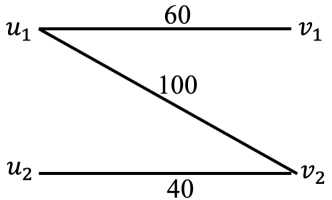
Figure 3: The graph for Example 2

.

5.3 Repairing a Fundamental Component

Definition 16.

At any point in the mechanism, for any connected component $C$ of $H$, $\min(C)$ will denote the smallest profit share of an essential vertex in $C$. We will say that $C$ has min on both sides if there is a vertex in $\mbox{\rm left}(C)$ as well as one in $\mbox{\rm right}(C)$ whose profit is $\min(C)$; if so, $C$ is said to be fully repaired. Otherwise, we will say that $C$ has min in $\mbox{\rm left}(C)$ ($\mbox{\rm right}(C)$) if there is a vertex in $\mbox{\rm left}(C)$ ($\mbox{\rm right}(C)$) whose profit is $\min(C)$.

The nature of the leximin order dictates that in order to leximin-improve the current core imputation, we must first try to increase the profit share of essential vertices having minimum profit, see also Remark 1. Let us start by studying this process for a fundamental component, $C$, which is not a unique imputation component. We call this process repairing $C$. Suppose $C$ has min in $\mbox{\rm left}(C)$, see Definition 16. Note that we cannot increase the profit of a single vertex in isolation, since the essential and viable edges of $C$ need to always be tight. Therefore there is only one way of repairing $C$, namely rotate $C$ clockwise, see Definition 17. If $C$ has min in $\mbox{\rm right}(C)$, we will need to rotate $C$ anti-clockwise.

Definition 17.

Let $C$ be a connected component in the tight subgraph. By rotating $C$ clockwise we mean continuously increasing the profit of $\mbox{\rm left}(C)$ and decreasing the profit of $\mbox{\rm right}(C)$ at unit rate, and by rotating $C$ anti-clockwise we mean continuously decreasing the profit of $\mbox{\rm left}(C)$ and increasing the profit of $\mbox{\rm right}(C)$ at unit rate.

How long can we carry out this repair? The answer is: until either $C$ has min on both sides or a subpar edge $e$ incident at $C$ goes exactly tight. In the first case, if we keep rotating $C$ beyond this point, $\min(C)$ will be attained by a vertex in $\mbox{\rm right}(C)$ only, if it was being rotated clockwise, and $\mbox{\rm left}(C)$ only, if it was being rotated anti-clockwise; furthermore the profit of this vertex will keep dropping, thereby making the imputation of $C$ lexicographically worse. Therefore we must stop repairing $C$; it is now fully repaired, see Definition 16. In the second case, if $C$ has min in $\mbox{\rm left}(C)$ ($\mbox{\rm right}(C)$) edge $e$ will be incident at a vertex at $\mbox{\rm right}(C)$($\mbox{\rm left}(C)$). At this point, the action to be taken depends on which component contains the other endpoint of $e$, see Section 6.

5.4 Three Key Ideas

We finally come to three key ideas which underly our mechanism.

1). As described above, leximin-improving the profit allocation of essential vertices of a fundamental component is straightforward. However, our task is much bigger: we need to iteratively improve the entire core imputation and terminate in the leximin imputation. Is there an orderly way of accomplishing this?

Towards this end, a central role is played by variable $\Omega$, which is initialized to the minimum profit share of an essential vertex under the starting core imputation, $(u,v)$. Thereafter, $\Omega$ is raised at unit rate until the mechanism terminates. Therefore, in effect $\Omega$ defines a notion of time. In a real implementation, $\Omega$ is not raised continuously; instead it is increased in spurts, since at each time, it is easy to compute the next value of $\Omega$ at which a significant event will take place. However, the description of the mechanism becomes much simpler if we assume that $\Omega$ is raised continuously, as is done below. A particularly succinct (and attractive) description is:

$\Omega$ keeps increasing and the entities of $G$ simply respond via rules given in Mechanism 1.

$\Omega$ provides a way of synchronizing the simultaneous repair of several components. Which components? A superficial answer is: the components in the set Active; a more in-depth answer is provided in Section 6 using Definition 19.

2). The second idea concerns the following question: Can tight subpar edges be added to $T$ when they go exactly tight? If not, why not and which tight subpar edges need to be added to $T$ and when?

Our mechanism adds a tight subpar edge to the tight subgraph only if it is legitimate, see Definition 18. This rule is critical for ensuring correctness of the mechanism, as shown in Example 3, after introducing more details of the mechanism.

3). As stated above, when a fundamental component, $C$, has min on both sides, the profit allocation of its essential vertices cannot be leximin-improved and $C$ is declared fully repaired. Now assume that a valid component, $D$, has min on both sides. Again, both clockwise and anti-clockwise rotations will lead to a worse profit allocation for its minimum profit essential vertices.

The third idea concerns the following question: For the situation described above, should we declare $D$ fully repaired? If not, why not and what is the right course of action?

It turns out that only a sub-component of $D$ can be declared to be fully repaired and identifying the right one is critical for ensuring correctness of the mechanism, as shown in Example 4. Furthermore, analogous issues arise when other events happen in the mechanism, see Section 6.2.1.

6 Mechanism for Leximin Core Imputation

In Step 1(a), an arbitrary core imputation, $(u,v)$, is found and in Step 1(b), $T$ is initialized to the set of essential and viable edges, thereby defining the starting tight subgraph $H=(V,T)$. For convenience, in Section 5, the starting tight set and the starting tight subgraph have been called $T_{0}$ and $H_{0}$, respectively. The connected components of $H_{0}$ are defined in Section 5.2.

In the initialization steps the connected components of $H_{0}$ are split among Frozen and Bin as follows: in Step 1(c), Frozen is initialized to the unique imputation components, see Definition 13, and in Step 1(d), Bin is initialized to the fundamental components, see Definition 14. By Corollary 1, all vertices of a fundamental component are essential. As the mechanism proceeds, the fundamental components move from Bin to one of the three sets, $\mbox{{Active}},\mbox{{Frozen}}$ and Fully-Repaired, and also back from Active to Bin. Each of these four sets has its own purpose, as described below. In Step 1(e), $\Omega$ is initialized to the minimum profit share of an essential vertex under $(u,v)$. The mechanism terminates when $(\mbox{{Bin}}\cup\mbox{{Active}})=\emptyset$.

The purpose of Active is to carry out repair of fundamental components using the principle summarized in Remark 1. As $\Omega$ increases, at some point one of three possible events may happen; they are given in Steps 2(a), 2(b) and 2(c) in Mechanism 1. It is important to point out that if several events happen simultaneously, they can be executed in any order, see also Remark 2. Furthermore, as described in Remark 3, execution of one such event may lead to a cascade of more such events which all need to be executed before raising $\Omega$.

The first event is that $\Omega$ may become equal to $\min(C)$, for some component $C\in\mbox{{Bin}}$. If so, in Step 2(a) $C$ gets moved from Bin to Active and it starts undergoing repair. The second and the third events deal with dual and primal updates and are described in detail in Sections 6.1 and 6.2, respectively. We next address the question raised in Section 5, namely which tight edges are added to $T$ and when.

Example 3.

In Figure 4, the solid edges are essential and dotted ones are subpar. Assume that the starting profit shares of the essential vertices $(u_{1},v_{1},u_{2},v_{2})$ are $(60,40,10,50)$, respectively. Since $v_{3}$ is a subpar vertex it is moved to Frozen and the two essential edges are moved to Bin. Also, $\Omega$ is initialized to $10$. Observe that subpar edge $(u_{1},v_{3})$ is tight at the start of the mechanism. The question is what is the “right” rule for adding a tight subpar edge $e$ to $T$? We study two rules:

Rule 1). Subpar edge $e$ is added to $T$ exactly when it goes tight.
If so, during Initialization, $(u_{1},v_{3})$ is added to $T$. At $\Omega=10$, $(u_{1},v_{1})$ is moved from Bin to Active. $\Omega$ is raised at unit rate and when it becomes $20$, subpar edge $(u_{1},v_{2})$ becomes exactly tight and is added to $T$ and fundamental component $(u_{2},v_{2})$ is moved from Bin to Active. Now, since $(u_{1},v_{3})$ is in $T$, the entire graph moves into Frozen, and the mechanism ends with the imputation $(60,40,20,40)$ for $(u_{1},v_{1},u_{2},v_{2})$.

Rule 2). Subpar edge $e$ is added to $T$ exactly when it is found to be legitimate, see Definition 18.
Under this rule, $(u_{1},v_{3})$ is not added to $T$ during Initialization. At $\Omega=10$, $(u_{1},v_{1})$ is moved from Bin to Active. When $\Omega=20$, subpar edge $(u_{1},v_{2})$ is found to be legitimate; it is added to $T$ and fundamental component $(u_{2},v_{2})$ is moved from Bin to Active. Now, the valid component consisting of edges $(u_{1},v_{1}),(u_{1},v_{2}),(u_{2},v_{2})$ undergoes repair. At $\Omega=30$, it has min on both sides and is moved into Fully-Repaired. Since $(\mbox{{Bin}}\cup\mbox{{Active}})=\emptyset$, the mechanism terminates with the imputation $(70,30,30,30)$ for $(u_{1},v_{1},u_{2},v_{2})$.

Rule 2 is the correct rule; its imputation leximin dominates that of Rule 1.

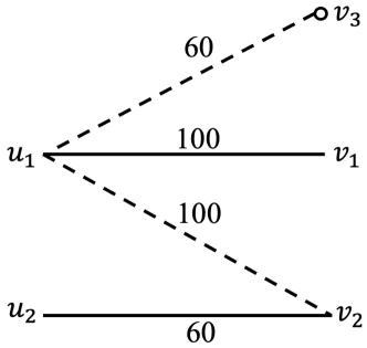
Figure 4: The graph for Example 3.

Definition 18.

Let $(i,j)$ be a tight subpar edge, with $i\in C$ and $j\in C^{\prime}$, where connected component $C\in\mbox{{Active}}$. We will say that $(i,j)$ is legitimate if either $C$ has min in $\mbox{\rm left}(C)$ and $i\in\mbox{\rm right}(C)$ or $C$ has min in $\mbox{\rm right}(C)$ and $i\in\mbox{\rm left}(C)$.

6.1 Dual Update: Repairing Valid Components

Section 6.2 describes the actions to be taken when an edge is found to be legitimate. One of these actions is that another fundamental component gets moved from Bin to the Active, thereby leading to a larger connected component. Each connected component in Active is called valid and its form is described in Definition 19.

Definition 19.

A valid component, $D$, consists of either a single fundamental component, $C_{0}$, or a set of fundamental components, $C_{0},C_{1},\ldots,C_{k}$, connected up via legitimate tight subpar edges. Because of the way $D$ is formed, it satisfies the following properties.

1. Shrink each fundamental component, $C_{i}$, to a single vertex, $w_{i}$, and if a legitimate edge runs between $C_{i}$ and $C_{j}$, then add an edge between $w_{i}$ and $w_{j}$. Then the resulting graph should form a tree, say $\tau$. Renumber components so $C_{0}$ is the root of this tree. If $w_{j}$ is a child of $w_{i}$ in $\tau$, then we will say that component $C_{j}$ is a child of $C_{i}$. The reflexive, transitive closure of the relation child will be called descendent. Thus all fundamental components in $D$ are descendent of $C_{0}$.

2. $\min(C_{0})=\min_{i=0}^{k}{\min(C_{i})}$, and $C_{0}$ does not have min on both sides.

3. First assume $C_{0}$ has min in $\mbox{\rm left}(C_{0})$. Each subpar edge of $D$ was legitimate at the time it was added to $T$. Therefore, by Definition 18, if component $C_{j}$ is a child of $C_{i}$ then the edge connecting them must run between $\mbox{\rm right}(C_{i})$ and $\mbox{\rm left}(C_{j})$, see Definition 16.

4. Next assume $C_{0}$ has min in $\mbox{\rm right}(C_{0})$. In this case, if component $C_{j}$ is a child of $C_{i}$ then the edge connecting them must run between $\mbox{\rm left}(C_{i})$ and $\mbox{\rm right}(C_{j})$.

5. The composite component $D$ does not have min on both sides. Clearly, $\min(D)=\min(C_{0})$.

The repair of a valid component $D$ is similar to that of a fundamental component, namely if $D$ has min in $\mbox{\rm left}(D)$ then rotate $D$ clockwise and otherwise rotate $D$ anti-clockwise, see Definition 17. When $D$ has min on both sides, it stops being a valid component and an appropriate sub-component, $\mbox{{Min-Sub1}}(D)$ is moved into Fully-Repaired, as described in Section 6.2.1. The purpose of Fully-Repaired is to hold fully repaired components, see Definition 16. The mechanism also decomposes $(D-\mbox{{Min-Sub1}}(D))$ into fundamental components and moves them back to Bin.

Remark 1.

As stated in Section 5, the nature of the leximin order dictates that in order to leximin-improve the current core imputation, we must first try to increase the profit share of essential vertices having minimum profit. Section 5 described this process for a fundamental component. The repair of a valid component, $D$, is also guided by the same consideration. Clearly, the root component, $C_{0}$, contains an essential vertex having minimum profit in $D$. Other fundamental components of $D$ may also contain such vertices; however, since $D$ does not have min on both sides, but these vertices will be on the same side as in $C_{0}$. $C_{0}$ dictates the kind of rotation, clockwise or anti-clockwise, which is applied to $D$. Observe that leximin-improving fundamental components containing minimum-profit essential vertices may require leximin-deteriorating other fundamental components of $D$.

6.2 Primal Update: Dealing with Legitimate Subpar Edges

Let $e$ be a legitimate subpar tight edge which runs between components $C$ and $C^{\prime}$, where $C\in\mbox{{Active}}$. The following four cases arise; the cases can be executed in any order. Let $D$ be the component obtained in Step 2(c)(v) by merging the newly tight edge $(i,j)$ together with components $C$ and $C^{\prime}$. For the exact definition of the minimum fully repaired sub-component of $D$ for each case, i.e., $\mbox{{Min-Sub1}}(D),\mbox{{Min-Sub2}}(D)$ and $\mbox{{Min-Sub3}}(D)$, see Section 6.2.1.

1. $C^{\prime}\in\mbox{{Active}}$. If so, it must be the case that $C$ and $C^{\prime}$ have min on opposite sides and the edge $(i,j)$ goes from one side of $C$ to the other side of $C^{\prime}$. As a result, $D$ has min on both sides. The mechanism moves the minimum fully repaired sub-component of $D$, $\mbox{{Min-Sub2}}(D)$ to Frozen and the fundamental components of $(D-\mbox{{Min-Sub2}}(D))$ to Bin.

2. $C^{\prime}\in\mbox{{Frozen}}$. In order to prevent $(i,j)$ from going under-tight, we need to stop the repair of $C$. This is done by moving $\mbox{{Min-Sub3}}(D)$ to Frozen and the fundamental components of $(D-\mbox{{Min-Sub3}}(D))$ to Bin.

3. $C^{\prime}\in\mbox{{Fully-Repaired}}$. If so, $\mbox{{Min-Sub3}}(D)$ is moved to Fully-Repaired and the fundamental components of $(D-\mbox{{Min-Sub3}}(D))$ are moved to Bin.

4. $C^{\prime}\in\mbox{{Bin}}$. In order to keep repairing $C$, we will move $C^{\prime}$ to Active, and start repairing $D$. Observe that if $C$ and $C^{\prime}$ have min on opposite sides and $\min(C^{\prime})=\Omega$, then $D$ is fully repaired and before raising $\Omega$, Step 2(b) needs to be executed.

Remark 2.

Note that if several edges become legitimate simultaneously, they can be handled in arbitrary order. This is true even if the edges are incident at the same component, e.g., suppose two edges, $e_{1}$ and $e_{2}$, incident at component $C$ become simultaneously legitimate, with $e_{1}$ connecting into Frozen and $e_{2}$ connecting into Fully-Repaired. If so, $C$ will end up in Frozen or Fully-Repaired depending on which edge is handled first. But in both cases no more changes will be made to the profit allocation of $C$ and therefore the core imputation computed will be the same.

When there are no more components left in $(\mbox{{Bin}}\cup\mbox{{Active}})$, the imputation computed is output in Step 3 and the mechanism terminates. In Section 6.3 we will prove that this imputation is indeed the leximin core imputation.

6.2.1 Determining the “Right” Sub-Component

The question of determining the “right” sub-component of a valid component arises at four steps in the mechanism; however they can be classified into three different types of situations, as described below. Example 4 illustrates the importance of determining the “right” sub-component for the first situation; it is easy to construct similar examples for the other situations as well.

We will need the following definition. Let $D$ be a valid component containing fundamental components $C_{i}$ and $C_{j}$, where $C_{j}$ is a descendent of $C_{i}$. Recall that descendent is the reflexive, transitive closure of the relation child, see Definition 19. We will say that fundamental component $C$ of $D$ is intermediate between $C_{i}$ and $C_{j}$ if $C$ is a descendent of $C_{i}$ and $C_{j}$ a descendent of $C$.

Step 2(b): A valid component $D$ has min on both sides. Let $C_{0}$ be the root fundamental component of $D$, see Definition 19. First assume that $C_{0}$ has min in $\mbox{\rm left}(C_{0})$. Since $D$ has min on both sides, there is at least one descendent, say $C_{i}$, of $C_{0}$ such that $C_{i}$ has min in $\mbox{\rm right}(C_{i})$ and $\min(C_{0})=\min(C_{i})$. Let $S$ be the set of all such descendents; clearly, $C_{i}\in S$. Then the sub-component of $D$ consisting of $C_{0}$, all components in $S$, and all components that are intermediate between $C_{0}$ and a component contained in $S$, together with the legitimate edges connecting these components, is the minimum fully repaired sub-component of $D$; we will denote it by $\mbox{{Min-Sub1}}(D)$.

Next assume that $C_{0}$ has min in $\mbox{\rm right}(C_{0})$. If so, in $S$ we will include all descendents, $C_{i}$ of $C_{0}$, such that $C_{i}$ has min in $\mbox{\rm left}(C_{i})$ and $\min(C_{0})=\min(C_{i})$. The rest of the construction is same as above. Finally, if $C_{0}$ has min on both sides, $S$ will include both types of descendents defined above.

The correct action to be taken in Step 2(b) is to move $\mbox{{Min-Sub1}}(D)$ to Fully-Repaired and decompose $(D-\mbox{{Min-Sub1}}(D))$ into fundamental components and move them back to Bin. See Example 4 for a detailed explanation.

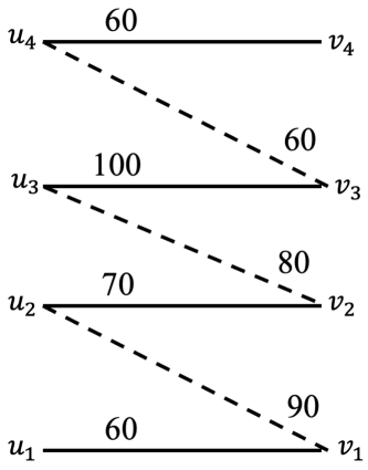
Figure 2: The graph for Example 4.

Example 4.

Figure 2 shows a valid component, say $D$, which has min on both sides at $\Omega=20$. Assume that the profit shares of its essential vertices ($u_{1},u_{2},u_{3},u_{4},v_{1},v_{2},v_{3},v_{4}$) are given by $(20,50,60,20,40,20,40,40)$, respectively. Moving all of $D$ to Fully-Repaired will lead to a core imputation which is not leximin, as shown next.

The minimum fully repaired sub-component of $D$, $\mbox{{Min-Sub1}}(D)$, consists of the graph induced on ($u_{1},u_{2},v_{1},v_{2}$), and it is added to Fully-Repaired in Step 2(b) of the mechanism. Furthermore, the fundamental components of $(D-\mbox{{Min-Sub1}}(D)$, namely ($u_{3},v_{3}$) and ($u_{4},v_{4}$) are moved them back to Bin.

Next, while $\Omega=20$, ($u_{4},v_{4}$) is moved back to Active in Step 2(a). Also, since $(u_{4},v_{3})$ is a legitimate edge, in Step 2(c)(iii), ($u_{3},v_{3}$) is also moved back to Active. The two together form valid component $D^{\prime}=(u_{3},u_{4},v_{3},v_{4})$. At this point, $\Omega$ starts increasing again. When $\Omega=30$, $D^{\prime}$ is found to have min on both sides. Furthermore, since $\mbox{{Min-Sub1}}(D^{\prime})=D^{\prime}$, it is moved into Fully-Repaired.

The final core imputation computed for essential vertices ($u_{1},u_{2},u_{3},u_{4},v_{1},v_{2},v_{3},v_{4}$) is given by $(20,50,70,30,40,20,30,30)$, respectively. This is a leximin core imputation.

Step 2(c)(iv): Edge $(i,j)$ connecting valid components $D$ and $D^{\prime}$, both in Active has gone tight. Let $R$ be the component obtained by merging $D,D^{\prime}$ and $(i,j)$ in Step 2(c)(ii). W.l.o.g. assume that $D$ has min in $\mbox{\rm left}(D)$ and $D^{\prime}$ has min in $\mbox{\rm right}(D^{\prime})$. If so, $i\in\mbox{\rm right}(D)$ and $j\in\mbox{\rm left}(D)$. Let $C_{0}$ and $C_{0}^{\prime}$ be the root fundamental components of $D$ and $D^{\prime}$, respectively and $C_{1}$ and $C_{1}^{\prime}$ be the fundamental components of $D$ and $D^{\prime}$ containing $i$ and $j$, respectively.

Then the sub-component of $R$ consisting of $C_{0},C_{1},C_{0}^{\prime},C_{1}^{\prime}$ and all components that are intermediate between $C_{0}$ and $C_{1}$ in $D$ and between $C_{0}^{\prime}$ and $C_{1}^{\prime}$ in $D^{\prime}$, together with the edge $(i,j)$, is the minimum fully repaired sub-component of $R$; we will denote it by $\mbox{{Min-Sub2}}(R)$. In Step 2(c)(iv), the mechanism moves $\mbox{{Min-Sub2}}(R)$ to Fully-Repaired and decomposes $(R-\mbox{{Min-Sub2}}(R))$ into fundamental components and moves them back to Bin.

Steps 2(c)(v) and 2(c)(vi): Edge $(i,j)$ connecting components $D$ and $D^{\prime}$ has gone tight, where $D^{\prime}\in\mbox{{Active}}$, and $D\in\mbox{{Frozen}}$ in Step 2(c)(v) and $D\in\mbox{{Fully-Repaired}}$ in Step 2(c)(vi). Let $R$ be the component obtained by merging $D,D^{\prime}$ and $(i,j)$ in Step 2(c)(ii). Let $C_{0}$ be the root fundamental component of $D^{\prime}$ and $C_{1}$ be the fundamental component of $D^{\prime}$ containing $i$.

Then the sub-component of $R$ consisting of $C_{0},C_{1}$ and all components that are intermediate between $C_{0}$ and $C_{1}$ in $D^{\prime}$, together with $D$ and the edge $(i,j)$, is the minimum fully repaired sub-component of $R$; we will denote it by $\mbox{{Min-Sub3}}(R)$.

The mechanism moves $\mbox{{Min-Sub3}}(R)$ to Frozen in Step 2(c)(v) and to Fully-Repaired in Step 2(c)(vi). In either step, it decomposes $(R-\mbox{{Min-Sub3}}(R))$ into fundamental components and moves them back to Bin.

Remark 3.

During the execution of Step 2(b) and Step 2(c), the mechanism may move a set of fundamental components back to Bin. For each such component, $C$, $\min(C)\geq\Omega$. If in fact $\min(C)=\Omega$, then to ensure proper synchronized running of the mechanism, $C$ needs to be moved back to Active before increasing $\Omega$. This may lead to the discovery of a legitimate edge incident at $C$, etc. Thus execution of one such event may lead to a cascade of such events which all need to be executed before raising $\Omega$.

6.3 Proof of Correctness of Mechanism 1

Our mechanism maintains the following key invariant:

Invariant: At any time $\Omega$ in the run of the mechanism, each fundamental component $C$ in Active and in Bin satisfies $\min(C)\geq\Omega$.

Lemma 4.

The mechanism maintains the Invariant.

Proof.

$\Omega$ is initialized to the minimum profit share of an essential vertex under the starting core imputation $(u,v)$ in Step 1(e), and at this time, each fundamental component $C$ with $\min(C)=\Omega$ is moved from Bin to Active. Therefore the invariant is satisfied at the beginning of the mechanism.

Below we will argue that each fundamental component $C$ which is moved from Active to Bin at time $\Omega$ satisfies $\min(C)\geq\Omega$. Moreover, before $\Omega$ is raised, all fundamental components $C$ in Bin satisfying $\min(C)=\Omega$ will be moved from Bin to Active. Therefore, at all times $\Omega$, Bin satisfies the invariant.

Assume that fundamental component $C$ moves from Bin to Active at time $\Omega$ in Step 2(a) or Step 2(c)(iii). If $\min(C)=\Omega$, the synchronization between the raising of $\Omega$ and the repair of $C$ ensures that $\min(C)=\Omega$ is maintained, until a new event happens.

For a valid component $D$ of $H$, which is in Active, we will say that $\min(D)\geq\Omega$ is challenged at time $\Omega$ if at time $\Omega$, $D$ has min on both sides; clearly, rotating $D$ anymore will damage the Invariant. However, at this time, $D$ is fully repaired and an appropriate sub-component of $D$ is moved from Active to Fully-Repaired in Step 2(c)(vi). The remaining fundamental components, say $C$, of $D$ are moved back to Bin. Since the latter satisfy $\min(C)\geq\Omega$, the fundamental components in Bin still satisfy the invariant. ∎

Lemma 5.

At any time $\Omega$ in the run of the mechanism, each valid component $D$ in Active satisfies $\min(D)=\min(C_{0})=\Omega$, where $C_{0}$ is the root fundamental component which grew into valid component $D$.

Proof.

Clearly the time $\Omega$ when $C_{0}$ moved from Bin to Active in Step 2(a), $\min(C_{0})=\Omega$. The synchronization between the raising of $\Omega$ and the repair of $C_{0}$ ensures that $\min(C_{0})=\Omega$ as long as $C_{0}\in\mbox{{Active}}$. Furthermore, by Lemma 4, any fundamental component $C^{\prime}$ which is linked, at time $\Omega^{\prime}$ say, to the connected component containing $C_{0}$ satisfies $\min(C^{\prime})\geq\Omega^{\prime}$. Therefore, $\min(D)=\min(C_{0})=\Omega$ as long as $D\in\mbox{{Active}}$. ∎

Lemma 6.

At any time $\Omega$ in the run of the mechanism, each valid component $D$ in Active satisfies the properties stated in Definition 19.

Proof.

Let $C_{0}$ be the root fundamental component of $D$ and assume that $C_{0}$ has min on the left; the other case is analogous. If so, the repair of $D$ involves a clockwise rotation and as shown in Lemma 5, while $D\in\mbox{{Active}}$, $min(D)=\min(C_{0})=\Omega$.

Assume that subpar edge $e$, incident at $D$, goes exactly tight at time $\Omega$. First observe that $e$ cannot form a cycle in $D$, i.e., the other endpoint of $e$ cannot be incident at $D$ — if so, the profit share of one endpoint of $e$ was increasing and the other was decreasing and therefore $e$ must remain over-tight. Next assume that the other endpoint of $e$ is incident at valid component $D^{\prime}\in\mbox{{Active}}$. For the same reason, $D^{\prime}$ cannot be undergoing a clockwise rotation. Therefore $D^{\prime}$ is undergoing an anti-clockwise rotation.

Let $C_{0}^{\prime}$ be the root fundamental component of $D^{\prime}$. Then $C_{0}^{\prime}$ must have min on the right, $\min(C_{0}^{\prime})=\Omega$, and the combined component consisting of $D,D^{\prime}$ and $e$ has min on both sides. Therefore its minimum fully repaired sub-component will be moved into Fully-Repaired in Step 2(c)(iv). Next assume that the other endpoint of $e$ is incident at a component $D^{\prime}$ which is in Frozen or Fully-Repaired. If so, similar actions will be taken in Step 2(c)(v) or Step 2(c)(vi), as described in Section 6.2.1.

The only case left is that the other endpoint of $e$ is incident at fundamental component $C\in\mbox{{Bin}}$. If so, the two endpoints of $e$ must be incident at $\mbox{\rm right}(D)$ and $\mbox{\rm left}(C)$. If so, $C$ will be moved into Active and $D$ satisfies the properties stated in Definition 19. ∎

At any time $\Omega=t$ in the run of the mechanism, let $V_{t}$ be the set of vertices of all components which are in $\mbox{{Frozen}}\cup\mbox{{Fully-Repaired}}$ and let $H_{t}$ denote the subgraph of $G$ induced on $V_{t}$. The proof of the next lemma follows from the fact that $H_{t}$ is not an arbitrary subgraph of $G$ – it is made up of unique imputation components and fundamental components of $G$.

Lemma 7.

The partitioning of vertices and edges of $H_{t}$ into essential, viable and subpar is a projection of their partitioning w.r.t. $G$.

Corollary 2.

The projection of the leximin core imputation of $G$ onto $H_{t}$ is the leximin core imputation for $H_{t}$.

Lemma 8.

At any time $\Omega=t$ in the run of the mechanism, the profit shares of vertices of $V_{t}$ form a leximin core imputation for the graph $H_{t}$.

Proof.

The reason underlying this lemma is that the “right” sub-component of a valid component is moved from Active to Frozen and Fully-Repaired, see Section 6.2.1. Suppose a valid component $D$ has min on both sides and $\mbox{{Min-Sub1}}(D)$ is the minimum fully repaired sub-component of $D$ which is moved into Fully-Repaired. Let $C_{0}$ be the root fundamental component of $D$; assume $C_{0}$ had min on the left when it moved into Active. There is a descendent $C_{0}^{\prime}$ of $C_{0}$ in $\mbox{{Min-Sub1}}(D)$ which has min on the right; clearly, $\min(C_{0})=\min(C_{0}^{\prime})=\min(D)$. Let $C$ be a fundamental component in $\mbox{{Min-Sub1}}(D)$ which is intermediate between $C_{0}$ and $C_{0}^{\prime}$.

Now, if $C$ has min on the left, then in order to leximin-improve its imputation, we must rotate it clockwise. However, in order that legitimate subpar edges of $\mbox{{Min-Sub1}}(D)$ don’t go under-tight, we will be forced to rotate clockwise all the fundamental components of $\mbox{{Min-Sub1}}(D)$ from $C$ to $C_{0}^{\prime}$, and this will lead to decreasing $\min(C_{0}^{\prime})$. Similarly, if $C$ has min on the right, then in order to leximin-improve its imputation, we will be forced to rotate anti-clockwise all the fundamental components of $\mbox{{Min-Sub1}}(D)$ from $C_{0}$ to $C$, and this will lead to decreasing $\min(C_{0})$. Since $\min(D)<\min(C)$, the leximin-gain in $C$ is over-shadowed by the leximin-loss in $\mbox{{Min-Sub1}}(D)$.

The other cases considered in Section 6.2.1 are similar, except when $\mbox{{Min-Sub3}}(D)$ gets moved into Frozen. In this case, $\mbox{{Min-Sub3}}(D)$ gets connected to a component in Frozen via legitimate edge $e$ which runs from $C_{0}^{\prime}$, a fundamental components of $\mbox{{Min-Sub3}}(D)$. Let $C_{0},C$ be as above, where $C$ is a fundamental component of $\mbox{{Min-Sub3}}(D)$ which is intermediate between $C_{0}$ and $C_{0}^{\prime}$. In this case, an anti-clockwise rotation of $C$ encounters the same issue as above. The difference arises with a clockwise rotation; this is prohibited since it will lead to legitimate edge $e$ going under-tight. ∎

For the sake of simplicity, let us make the assumption that the weights of edges of $G$ are integral. Note that this is without loss of generality, since we already assumed that the edge weights are rational, see Definition 2.

Definition 20.

Let $(u^{\alpha},v^{\alpha})$ denote the leximin core imputation and let $a_{1}<a_{2}<\ldots<a_{k}$ be the distinct profit shares assigned by it to essential vertices; of course several vertices may have the same profit share. For $1\leq l\leq k$, let $W_{l}\subseteq(U\cup V)$ denote the set of vertices whose profit share is $a_{l}$. We will say that a given core imputation is $\mbox{{Leximin}}(l)$-processed if the profit shares of vertices in $W_{1}\cup\ldots\cup W_{l}$ are consistent with the leximin core imputation.

The following key theorem captures the way Mechanism 1 makes progress.

Theorem 5.

Let $\epsilon>0$ be a small number. For $1\leq l\leq k$, when $\Omega=a_{l}+\epsilon$, the current core imputation is $\mbox{{Leximin}}(l)$-processed.

Proof.

Consider the time $\Omega=a_{l}+\epsilon$. By Lemma 8, the profit shares of vertices of $V_{t}$, where $t=a_{l}+\epsilon$, form a leximin core imputation for the graph $H_{t}$ defined above. Since by Corollary 2, the leximin core imputation for $H_{t}$ is the projection of the leximin core imputation of $G$ onto $H_{t}$, we conclude that the profit shares of vertices of ($\mbox{{Frozen}}\cup\mbox{{Fully-Repaired}}$) are the same as those of the corresponding vertices of $G$ in the leximin core imputation.

Next we will prove that $(W_{1}\cup\ldots\cup W_{l})\subseteq(\mbox{{Frozen}}\cup\mbox{{Fully-Repaired}})$, thereby establishing the lemma. By Lemma 4, the mechanism maintains the Invariant and therefore each fundamental component $C$ in $(\mbox{{Active}}\cup\mbox{{Bin}})$ satisfies $\min(C)\geq a_{l}+\epsilon$. Consider an essential vertex $v\in(\mbox{{Active}}\cup\mbox{{Bin}})$. Since the current imputation found by the mechanism is a core imputation of $G$, the profit share of $v$ in the leximin core imputation must be $\geq a_{l}+\epsilon$. Therefore no vertex of $(W_{1}\cup\ldots\cup W_{l})$ is in $(\mbox{{Active}}\cup\mbox{{Bin}})$, thereby proving the theorem. ∎

Corollary 3.

Mechanism 1 terminates by time $\Omega=a_{k}+\epsilon$ with a leximin core imputation.

As a consequence of Lemma 9, in Theorem 5, picking $0<\epsilon<{1\over 2}$ suffices.

Lemma 9.

The leximin core imputation is half-integral.

Proof.

Assume that the weight $w_{e}$ of an essential edge $e$ is an odd number. If $e$ achieves min on both sides, then the profit shares of its endpoints will be half integral, i.e., ${{w_{e}}\over 2}$. A similar event can occur when a component has min on both sides. There is no other step in the mechanism which splits the profit share of a vertex any further. The lemma follows. ∎

In order to put a bound on the running time of Mechanism 1, let us partition its run into epochs. The first epoch starts with the start of the mechanism and an epoch ends when a fundamental component gets moved to $(\mbox{{Frozen}}\cap\mbox{{Fully-Repaired}})$, i.e., in Step 2(b), 2(c)(iv), 2(c)(v) or 2(c)(vi).

Lemma 10.

Mechanism 1 executes $O(n^{2})$ steps.

Proof.

Since each epoch terminates with moving at least two vertices to $(\mbox{{Frozen}}\cap\mbox{{Fully-Repaired}})$, Mechanism 1 terminates in $O(n)$ epochs. At the end of an epoch, some fundamental components may move from Active to Bin; however, their number is bounded by $n$. Since each step between two epochs involves moving at least one fundamental component move from Bin to Active, the number of such steps is $O(n)$, thereby proving the lemma. ∎

The only other computation needed in Mechanism 1 is to discretize the raising of $\Omega$, i.e., to determine the next time when an event will take place. This can clearly be done in linear time in $m$, the number of edges in $G$. Hence we get:

Theorem 6.

Mechanism 1 runs in polynomial time.

We leave the problem of optimizing the running time of Mechanism 1.

7 Mechanism for Leximax Core Imputation

Mechanism 2 computes the leximax core imputation for the assignment game, $G=(U,V,E),\ w:E\rightarrow\mathcal{Q}_{+}$. It differs from Mechanism 1 in the following ways:

1. In Step 1(e), $\Omega$ is initialized to the maximum profit share of an essential vertex under the initial core imputation $(u,v)$ computed in Step 1(a).

2. Whereas in Mechanism 1, $\Omega$ is raised at unit rate, in Mechanism 2, it is lowered at unit rate.

3. Definition 21 plays a role analogous to that of Definition 16. Furthermore, for Mechanism 2, we will say that component $C$ is fully repaired if it has max on both sides.

4. Repairing a Component: If component $C$ has max in $\mbox{\rm left}(C)$, then $C$ needs to be rotated anti-clockwise and if it has max in $\mbox{\rm right}(C)$, it needs to be rotated clockwise.

5. The previous change will change the definition of valid component appropriately. Furthermore, the definitions of $\mbox{{Min-Sub1}},\mbox{{Min-Sub2}}$ and Min-Sub3 will change appropriately and we will denote the resulting sub-components by $\mbox{{Max-Sub1}},\mbox{{Max-Sub2}}$ and Max-Sub3, respectively.

6. The proofs of correctness and running time of Mechanism 2 are analogous to that of Mechanism 1.

Definition 21.

At any point in the mechanism, for any connected component $C$ of $H$, $\max(C)$ will denote the largest profit share of an essential vertex in $C$. We will say that $C$ has max on both sides if there is a vertex in $\mbox{\rm left}(C)$ as well one in $\mbox{\rm right}(C)$ whose profit is $\max(C)$. Otherwise, we will say that $C$ has max in $\mbox{\rm left}(C)$ $(\mbox{\rm right}(C))$ if there is a vertex in $\mbox{\rm left}(C)$ ($\mbox{\rm right}(C)$) whose profit is $\max(C)$.

Theorem 7.

Mechanism 2 computes the leximax core imputation in polynomial time.

8 Discussion

Here are some interesting questions regarding leximin and leximax core imputations:

1. Characterize the points of the polytope of optimal dual solutions to LP (3.1) where the leximin and leximax core imputations lie, see Section 5.1.

2. As shown in Section 4, in general, the leximin and leximax core imputations of the assignment game are different, calling for a study of their pros and cons. Properties of their convex combinations are also worth exploring.

9 Acknowledgements

I wish to thank Atila Abdulkadiroglu, Rohith Gangam, Naveen Garg and Hervé Moulin for valuable discussions.

References

- [AM85] Robert J Aumann and Michael Maschler. Game theoretic analysis of a bankruptcy problem from the talmud. Journal of economic theory, 36(2):195–213, 1985.
- [Arr12] Kenneth J Arrow. Social choice and individual values, volume 12. Yale university press, 2012.
- [Bir37] Garrett Birkhoff. Rings of sets. Duke Mathematical Journal, 3(3):443–454, 1937.
- [Che10] Christine T Cheng. Understanding the generalized median stable matchings. Algorithmica, 58:34–51, 2010.
- [CMS11] Christine Cheng, Eric McDermid, and Ichiro Suzuki. Center stable matchings and centers of cover graphs of distributive lattices. In Automata, Languages and Programming: 38th International Colloquium, ICALP 2011, Zurich, Switzerland, July 4-8, 2011, Proceedings, Part I 38, pages 678–689. Springer, 2011.
- [DIN99] Xiaotie Deng, Toshihide Ibaraki, and Hiroshi Nagamochi. Algorithmic aspects of the core of combinatorial optimization games. Mathematics of Operations Research, 24(3):751–766, 1999.
- [DR89] Bhaskar Dutta and Debraj Ray. A concept of egalitarianism under participation constraints. Econometrica: Journal of the Econometric Society, pages 615–635, 1989.
- [EIV23] Federico Echenique, Nicole Immorlica, and V Vazirani. Two-sided markets: Stable matching. In Federico Echenique, Nicole Immorlica, and V Vazirani, editors, Online and matching-based market design, chapter 1. Cambridge University Press, 2023.
- [GH81] Daniel Granot and Gur Huberman. Minimum cost spanning tree games. Mathematical programming, 21(1), 1981.
- [GH84] Daniel Granot and Gur Huberman. On the core and nucleolus of minimum cost spanning tree games. Mathematical programming, 29(3):323–347, 1984.
- [GS62] David Gale and Lloyd S Shapley. College admissions and the stability of marriage. The American Mathematical Monthly, 69(1):9–15, 1962.
- [IL86] Robert W Irving and Paul Leather. The complexity of counting stable marriages. SIAM Journal on Computing, 15(3):655–667, 1986.
- [ILG87] Robert W Irving, Paul Leather, and Dan Gusfield. An efficient algorithm for the “optimal” stable marriage. Journal of the ACM (JACM), 34(3):532–543, 1987.
- [KP08] Tamás Király and Júlia Pap. Total dual integrality of rothblum’s description of the stable-marriage polyhedron. Mathematics of Operations Research, 33(2):283–290, 2008.
- [KS20] Zhuan Khye Koh and Laura Sanità. An efficient characterization of submodular spanning tree games. Mathematical Programming, 183(1):359–377, 2020.
- [KZ82] Ehud Kalai and Eitan Zemel. Totally balanced games and games of flow. Mathematics of Operations Research, 7(3):476–478, 1982.
- [LP86] L. Lovász and M.D. Plummer. Matching Theory. North-Holland, Amsterdam–New York, 1986.
- [Mou91] Hervé Moulin. Axioms of cooperative decision making. Number 15. Cambridge university press, 1991.
- [Mou14] Hervé Moulin. Cooperative microeconomics: a game-theoretic introduction, volume 313. Princeton University Press, 2014.
- [Mou19] Hervé Moulin. Fair division in the internet age, volume 11. Annual Reviews, 2019.
- [NZKI97] Hiroshi Nagamochi, Dao-Zhi Zeng, Naohiśa Kabutoya, and Toshihide Ibaraki. Complexity of the minimum base game on matroids. Mathematics of Operations Research, 22(1):146–164, 1997.
- [Rot92] Uriel G Rothblum. Characterization of stable matchings as extreme points of a polytope. Mathematical Programming, 54(1):57–67, 1992.
- [SS71] Lloyd S Shapley and Martin Shubik. The assignment game I: The core. International Journal of Game Theory, 1(1):111–130, 1971.
- [TS98] Chung-Piaw Teo and Jay Sethuraman. The geometry of fractional stable matchings and its applications. Mathematics of Operations Research, 23(4):874–891, 1998.
- [Vat89] John H Vande Vate. Linear programming brings marital bliss. Operations Research Letters, 8(3):147–153, 1989.
- [Vaz22] Vijay V Vazirani. New characterizations of core imputations of matching and b-matching games. In 42nd IARCS Annual Conference on Foundations of Software Technology and Theoretical Computer Science (FSTTCS 2022). Schloss Dagstuhl-Leibniz-Zentrum für Informatik, 2022.