OptEx: Expediting First-Order Optimization with Approximately
Parallelized Iterations

Abstract

First-order optimization (FOO) algorithms are pivotal in numerous computational domains such as machine learning and signal denoising. However, their application to complex tasks like neural network training often entails significant inefficiencies due to the need for many sequential iterations for convergence. In response, we introduce first-order optimization expedited with approximately parallelized iterations (OptEx), the first framework that enhances the efficiency of FOO by leveraging parallel computing to mitigate its iterative bottleneck. OptEx employs kernelized gradient estimation to make use of gradient history for future gradient prediction, enabling parallelization of iterations—a strategy once considered impractical because of the inherent iterative dependency in FOO. We provide theoretical guarantees for the reliability of our kernelized gradient estimation and the iteration complexity of SGD-based OptEx, confirming that estimation errors diminish to zero as historical gradients accumulate and that SGD-based OptEx enjoys an effective acceleration rate of $\Theta(\sqrt{N})$ over standard SGD given parallelism of $N$. We also use extensive empirical studies, including synthetic functions, reinforcement learning tasks, and neural network training across various datasets, to underscore the substantial efficiency improvements achieved by OptEx.

1 Introduction

First-order optimization (FOO) algorithms, e.g., stochastic gradient descent (SGD) (Robbins & Monro, 1951), Nesterov Accelerated Gradient (NGA) (Nesterov, 1983), AdaGrad (Duchi et al., 2011), Adam (Kingma & Ba, 2014) and etc., have already been the cornerstone of many computational disciplines, driving advancements in areas ranging from signal denoising (Ostrovskii & Harchaoui, 2018) to machine learning (Lan, 2020). These algorithms, widely known for their straightforward form of iterative gradient-based updates, are fundamental in solving both simple and intricate optimization problems. However, their application often encounters substantial challenges in practice, especially when addressing complex functions that not only are expensive in evaluating their function values and gradients but also necessitate a large number of sequential iterations to converge, e.g., neural network training (Krizhevsky et al., 2012), resulting in considerable time demands in practice.

Parallel computing has been utilized to significantly enhance the computational efficiency of FOO, with prevailing strategies focusing on reducing the evaluation time for function values and gradients per FOO iteration, consequently lowering the overall time expense in optimization (Assran et al., 2020). In the specific area of deep neural network training, techniques such as data parallelism (Krizhevsky et al., 2012), model parallelism (Dean et al., 2012), and pipeline parallelism (Harlap et al., 2018; Huang et al., 2019) have been effectively employed to decrease the evaluation time of loss function by processing multiple input samples and network components concurrently. However, the specialized nature of these methods for neural network training limits their broader applicability, for instance, in hyper-parameter tuning (Yu & Zhu, 2020). This restriction underscores the need to explore the potential for parallelizing sequential iterations within the FOO framework, which could further enhance the optimization efficiency of FOO with wider practical applicability. To our knowledge, there has been limited research on developing iteration parallelism for FOO algorithms.

However, the development of iteration parallelism in FOO encounters two principal challenges. Firstly and foremost, the inherent iterative dependency of FOO where the output of each iteration is the input of the next, poses a significant barrier to independent and concurrent iteration advancement, thereby making it impossible to realize iteration parallelism within the FOO framework. Secondly, if this iteration parallelism is indeed feasible, the necessary theoretical guarantees for confirming its ability to definitively accelerate FOO algorithms are still largely unexplored in existing research.

To this end, we develop a novel framework called first-order optimization expedited with approximately parallelized iterations (OptEx) that is capable of bypassing the challenge of inherent iterative dependency in FOO and therefore make parallelized iterations in FOO possible. Specifically, our framework begins with a novel kernelized gradient estimation strategy, which utilizes the history of gradients during optimization to predict the gradients for any input within the domain such that these estimated gradients can be used in FOO algorithms to determine the input for the next iteration. Furthermore, to enhance the efficiency of this kernelized gradient estimation, we also introduce the technique of separable kernel function and local history of gradients for our gradient estimation (Sec. 4.1). We then naturally employ standard FOO algorithms with these estimated gradients to determine the initial inputs for the next $N$ sequential iterations, namely proxy updates, to approximate the ground-truth sequential updates and consequently bypass the iteration dependency in FOO (Sec. 4.2). Lastly, we complete our parallelized iterations for FOO by using parallel computing to run standard FOO algorithms over these $N$ inputs obtained from our proxy updates concurrently (Sec. 4.3).

In this work, apart from establishing our innovative OptEx framework, we also furnish rigorous theoretical guarantees and extensive empirical studies underpinning its efficacy. Specifically, we give a theoretical bound for the estimation error in our kernelized gradient estimation. Remarkably, this error is shown to asymptotically approach zero as the number of historical gradients increases, ranging across a broad spectrum of kernel functions. This finding suggests that our kernelized gradient estimation facilitates effective proxy updates for parallelizing iterations in FOO (Sec.5.1). Building on this, we delineate both upper and lower bounds for iteration complexity in our SGD-based OptEx. This framework typically reduces the iteration complexity of standard FOO algorithms at a rate of $\Theta(\sqrt{N})$ with a parallelism of $N$, leading to a corresponding effective acceleration rate of $\Theta(\sqrt{N})$ over standard SGD algorithm (Sec.5.2). Finally, through extensive empirical studies, including the optimization of synthetic functions, reinforcement learning tasks, and neural network training on both image and text datasets, we demonstrate the consistent ability of our OptEx to expedite existing FOO algorithms (Sec. 6).

To summarize, our contribution in this work includes:

• To the best of our knowledge, we are the first to develop a general framework OptEx that can leverage parallel computing to approximately parallelize the sequential iterations in FOO, thereby considerably reducing the sequential iteration complexity of FOO algorithms.

• We provide the first upper and lower iteration complexity bound for our SGD-based OptEx, which gives an effective acceleration rate of $\Theta(\sqrt{N})$ that is achievable by our SGD-based OptEx with parallelism of $N$.

• We conduct extensive empirical studies, including the optimization of synthetic function, reinforcement learning tasks, and neural network training on both image and text datasets, to adequately support the efficacy of our OptEx framework.

2 Related Work

Reduction of Iteration Complexity.

To enhance the efficiency of FOO algorithms, various techniques have been developed to diminish their iteration complexity. Specifically, variance reduction strategies (Johnson & Zhang, 2013; Zhou et al., 2018; Sebbouh et al., 2019) have been proposed to accelerate stochastic optimization, which can effectively reduce the gradient variance and align the iteration complexity of SGD with that of gradient descent (GD) in expectations. These strategies usually yield significant improvements in high-variance problems whereas their compelling performance is hard to extend to low-variance scenarios let alone deterministic contexts. In parallel, adaptive gradient methods, such as AdaGrad (Duchi et al., 2011), Adam (Kingma & Ba, 2014), and AdaBelief (Zhuang et al., 2020), have been introduced to dynamically choose the optimal learning rates for a better-performing optimization where fewer iterations are required for convergence. Furthermore, acceleration techniques like the Nesterov method (Nesterov, 1983) and momentum-based updates (Liu et al., 2020) have also been proven to be able to reduce iteration complexity for GD and SGD efficiently. Orthogonal to these established methodologies, our paper introduces parallel computing as a distinct and innovative strategy to further decrease the iteration complexity of FOO algorithms. This approach not only stands independently but also offers potential for synergistic integration with existing methods, promising enhanced optimization outcomes.

Reduction of Time Complexity for Each Iteration.

In the realm of enhancing the computational efficiency of FOO through reducing their time complexity for each iteration, parallel computing has emerged as a rescue. Particularly in deep neural network training, methodologies such as data parallelism (Krizhevsky et al., 2012), model parallelism (Dean et al., 2012), and pipeline parallelism (Harlap et al., 2018; Huang et al., 2019), have been adeptly applied to reduce the computational time for each evaluation of the loss function by simultaneously processing various input samples and network components. Yet, the tailored nature of these methods to neural network training constrains their application to wider contexts. Contradictory to these case-specified solutions, this paper proposes to leverage parallel computing for iteration parallelism within the FOO framework, which can enhance the efficiency of FOO while maintaining broad practical applicability.

3 Problem Setup and Challenge of Parallelized Iterations in FOO

In this paper, we aim to enhance the optimization efficiency of the following stochastic minimization problem by leveraging parallel computing with parallelism of $N$:

$$\min_{{\bm{\theta}}\in{\mathbb{R}}^{d}}F({\bm{\theta}})\triangleq\mathbb{E}\left[f({\bm{\theta}},{\bm{x}})\right]$$ (1)

where the stochasticity comes from the random variable ${\bm{x}}$ and $\nabla f({\bm{\theta}},{\bm{x}})$ is assumed to follow a Gaussian distribution, i.e., $\nabla f({\bm{\theta}},{\bm{x}})\sim{\mathcal{N}}(\nabla F({\bm{\theta}}),\sigma^{2}{\mathbf{I}})$ for any ${\bm{\theta}}\in{\mathbb{R}}$, which has been widely used in the literature (Luo et al., 2018; He et al., 2019; Wu et al., 2021). Besides, we adopt a common assumption that $\nabla F$ is sampled from a Gaussian process, i.e., $\nabla F\sim\mathcal{GP}({\bm{0}},{\mathbf{K}}(\cdot,\cdot))$ (Rasmussen & Williams, 2006; Shu et al., 2023a, b). Of note, (1) has found extensive applications in practice, such as neural network training (Goodfellow et al., 2016) and reinforcement learning (Sutton & Barto, 2018). Importantly, although our primary focus is on stochastic optimization, our proposed method is also applicable to deterministic optimization, as shown in Sec. 6.

Note that existing FOO algorithms commonly optimize (1) in an iterative and sequential manner:

$${\bm{\theta}}_{t+1}=\text{{FO-OPT}{}}({\bm{\theta}}_{t},\nabla f({\bm{\theta}}_{t},{\bm{x}}),{\bm{\lambda}}_{t})$$ (2)

where $t$ is the iteration number and ${\bm{\lambda}}_{t}$ represents the hyper-parameters of first-order optimizer FO-OPT e.g., learning rate $\eta_{t}$ for SGD.

Ideally, if parallel computing can be leveraged to parallelize the sequential iterations in FOO, it could lead to a marked improvement in its optimization efficiency. Unfortunately, there is an inherent iterative dependency in FOO, that is, the output of each iteration $t$ (e.g., ${\bm{\theta}}_{t}$) is the input of the next iteration $t+1$. Such an iterative and sequential process makes it nearly impossible to parallelize the iterations for established FOO algorithms.

4 Expediting First-Order Optimization with Approximately Parallelized Iterations

To this end, we develop a novel and general framework in Algo. 1, namely first-order optimization expedited with approximately parallelized iterations (OptEx), to overcome the inherent iterative dependency in FOO and hence facilitate the realization of parallelized iterations therein. We first propose a kernelized gradient estimation method with the technique of separable kernel function and local history of gradient to efficiently and effectively estimate the gradient at an input in the domain using only a subset of gradient history (Sec. 4.1). With these estimated gradients, we then utilize standard FOO algorithms to approximate the initial inputs for their next $N$ sequential iterations (Sec.4.2), which thus bypasses the inherent iterative dependency in FOO. Lastly, we finish our approximately parallelized iterations by leveraging parallel computing to run standard FOO algorithms on these $N$ initial inputs concurrently (Sec. 4.3).

Algorithm 1 OptEx

Input: FO-OPT with hyper-parameters ${\bm{\lambda}}$, kernel $k(\cdot,\cdot)$, iterations $T$, parallelism $N$, initialization ${\bm{\theta}}_{0}$, gradient history ${\mathcal{G}}=\varnothing$

for sequential iteration $t\in[T]$ do

2       Initialization: ${\bm{\theta}}_{t,0}\leftarrow{\bm{\theta}}_{t-1}$ Update estimator ${\bm{\mu}}_{t}({\bm{\theta}})$ from (4.1) using ${\mathcal{G}}$ for proxy step $s\in[N-1]$ do

3             ${\bm{\theta}}_{t,s}\leftarrow\text{{FO-OPT}{}}({\bm{\theta}}_{t,s-1},{\bm{\mu}}_{t}({\bm{\theta}}_{t,s-1}),{\bm{\lambda}}_{t,s-1})$

4      for process $i\in[N]$ in parallel do

5             ${\bm{\theta}}^{(i)}_{t}\leftarrow\text{{FO-OPT}{}}({\bm{\theta}}_{t,i-1},\nabla f({\bm{\theta}}_{t,i-1},{\bm{x}}),{\bm{\lambda}}_{t,i-1})$ ${\mathcal{G}}\leftarrow{\mathcal{G}}\cup\{({\bm{\theta}}_{t,i-1},\nabla f({\bm{\theta}}_{t,i-1}),{\bm{x}})\}$

6      ${\bm{\theta}}_{t}\leftarrow\operatorname*{arg\,min}_{{\bm{\theta}}_{t}^{(i)}\in\{{\bm{\theta}}_{t}^{(j)}\}_{j=1}^{N}}f({\bm{\theta}}^{(i)}_{t},{\bm{x}})$ or alternatively ${\bm{\theta}}_{t}\leftarrow\operatorname*{arg\,min}_{{\bm{\theta}}_{t}^{(i)}\in\{{\bm{\theta}}_{t}^{(j)}\}_{j=1}^{N}}\left\|\nabla f({\bm{\theta}}^{(i)}_{t},{\bm{x}})\right\|$

4.1 Kernelized Gradient Estimation

As discussed in our Sec. 3, $\nabla F$ is assumed to be sampled from a Gaussian process, i.e., $\nabla F\sim\mathcal{GP}({\bm{0}},{\mathbf{K}}(\cdot,\cdot))$ with kernel function ${\mathbf{K}}$. Then, for every sequential iteration $t$ of Algo. 1, conditioned on the history of gradients during optimization ${\mathcal{G}}\triangleq\{({\bm{\theta}}_{\tau},\nabla f({\bm{\theta}}_{\tau},{\bm{x}})\}_{\tau=1}^{N(t-1)}$ , $\nabla F$ follows the posterior Gaussian process: $\nabla F\sim\mathcal{GP}\left({\bm{\mu}}_{t}(\cdot),{\bm{\Sigma}}_{t}^{2}(\cdot,\cdot)\right)$ with the mean function ${\bm{\mu}}_{t}(\cdot)$ and the covariance function ${\bm{\Sigma}}_{t}^{2}(\cdot,\cdot)$ defined as below (Rasmussen & Williams, 2006):

$${\bm{\mu}}_{t}({\bm{\theta}}) \triangleq{\mathbf{V}}^{\top}_{t}({\bm{\theta}})\left({\mathbf{U}}_{t}+\sigma^{2}{\mathbf{I}}\right)^{-1}\mathrm{vec}({\mathbf{G}}^{\top}_{t})$$ (3)

$${\bm{\Sigma}}_{t}^{2}({\bm{\theta}},{\bm{\theta}}^{\prime}) \triangleq{\mathbf{K}}\left({\bm{\theta}},{\bm{\theta}}^{\prime}\right)-{\mathbf{V}}^{\top}_{t}({\bm{\theta}})\left({\mathbf{U}}_{t}+\sigma^{2}{\mathbf{I}}\right)^{-1}{\mathbf{V}}_{t}\left({\bm{\theta}}^{\prime}\right)$$

where $\mathrm{vec}(\cdot)$ vectorizes a matrix into a column vector, ${\mathbf{G}}_{t}\triangleq[\nabla f({\bm{x}},{\bm{\theta}}_{\tau})]_{\tau=1}^{N(t-1)}$ is a $d\times N(t-1)$-dimensional matrix, ${\mathbf{V}}^{\top}_{t}({\bm{\theta}})\triangleq\left[{\mathbf{K}}({\bm{\theta}},{\bm{\theta}}_{\tau})\right]_{\tau=1}^{N(t-1)}$ is a $d\times N(t-1)d$-dimensional matrices, and ${\mathbf{U}}_{t}\triangleq\left[{\mathbf{K}}({\bm{\theta}}_{\tau},{\bm{\theta}}_{\tau^{\prime}})\right]_{\tau,\tau^{\prime}=1}^{N(t-1)}$ is a $N(t-1)d\times N(t-1)d$-dimensional matrices. As a result, we can make use of ${\bm{\mu}}_{t}(\cdot)$ to estimate the gradient at any input ${\bm{\theta}}\in{\mathbb{R}}^{d}$, that is,

$$\nabla F({\bm{\theta}})\approx\mu_{t}({\bm{\theta}})$$ (4)

where variance ${\bm{\Sigma}}^{2}({\bm{\theta}})\triangleq{\bm{\Sigma}}^{2}({\bm{\theta}},{\bm{\theta}})$ can be used to measure the quality of this gradient estimation in a principled way, which will be theoretically supported in our Sec. 5.1.

However, each sequential iteration $t+1$ of Algo. 1 with (3) incurs a computational complexity of ${\mathcal{O}}(d^{3}t^{3}(N-1))$, along with a space complexity of ${\mathcal{O}}(Ntd)$. Practically, this presents a significant challenge, as the variable $t$ escalates during the optimization process. This escalation becomes particularly burdensome in scenarios requiring a large number of sequential iterations for convergence, such as in neural network training (Krizhevsky et al., 2012). To mitigate these complexity issues, we introduce two techniques: the separable kernel function and the local history of gradients, to reduce both the computational and space complexities associated with kernelized gradient estimation, thereby enhancing its efficiency and practical applicability.

Separable Kernel Function.

Let ${\mathbf{K}}(\cdot,\cdot)=k(\cdot,\cdot)\,{\mathbf{I}}$ where $k(\cdot,\cdot)$ produces a scalar value and ${\mathbf{I}}$ is a $d\times d$ matrix and define the $d\times N(t-1)$-dimensional matrix, the $N(t-1)$-dimensional vector ${\bm{k}}_{t}^{\top}({\bm{\theta}})\triangleq[k({\bm{\theta}},{\bm{\theta}}_{\tau})]_{\tau=1}^{N(t-1)}$, and $N(t-1)\times N(t-1)$-dimensional matrix ${\mathbf{K}}_{t}\triangleq[k({\bm{\theta}}_{\tau},{\bm{\theta}}_{\tau^{\prime}})]_{\tau=\tau^{\prime}=1}^{N(t-1)}$, we can prove that the multi-output Gaussian process in (3) can then be decoupled into independent Gaussian processes as shown in Prop. 4.1 (proof in Appx. A.1).

Proposition 4.1.

Let ${\mathbf{K}}(\cdot,\cdot)=k(\cdot,\cdot)\,{\mathbf{I}}$, the posterior mean and covariance in (3) become

$${\bm{\mu}}_{t}({\bm{\theta}}) =\left[\left({\bm{k}}_{t}^{\top}({\bm{\theta}})\left({\mathbf{K}}_{t}+\sigma^{2}{\mathbf{I}}\right)^{-1}\right){\mathbf{G}}_{t}\right]^{\top}$$

$${\bm{\Sigma}}_{t}^{2}({\bm{\theta}},{\bm{\theta}}^{\prime}) =\left(k({\bm{\theta}},{\bm{\theta}}^{\prime})-{\bm{k}}_{t}^{\top}({\bm{\theta}})\left({\mathbf{K}}_{t}+\sigma^{2}{\mathbf{I}}\right)^{-1}{\bm{k}}_{t}({\bm{\theta}}^{\prime})\right){\mathbf{I}}\ .$$

Prop. 4.1 shows that with a separable kernel function, specifically ${\mathbf{K}}(\cdot,\cdot)=k(\cdot,\cdot)\,{\mathbf{I}}$, the multi-output Gaussian process in a $d$-dimensional space can be effectively decoupled into $d$ independent single-output Gaussian processes. Each of these processes results from the same scalar kernel function $k$, leading to a uniform posterior form. This therefore considerably diminishes the computational complexity, now quantified as ${\mathcal{O}}(t^{3}(N-1))$, resulting in a more computationally efficient gradient estimation in practice.

Local History of Gradients.

Conventional FOO algorithms predominantly operate by optimizing within a localized region neighboring the initial input ${\bm{\theta}}_{0}$. Correspondingly, our Algo. 1 only necessitates precise gradient estimation within this local region. In this context, the utilization of a local gradient history is posited as sufficiently informative for effective kernelized gradient estimation, as supported by the theoretical results in (Lederer et al., 2019) and corroborated by the empirical evidence in Sec. 6. Thus, rather than relying on the complete gradient history, our method proposes to use a localized gradient history of size $T_{0}$ that neighbors ${\bm{\theta}}$ to estimate the gradient at ${\bm{\theta}}$. This strategic modification results in a substantial reduction of computational complexity to ${\mathcal{O}}(T_{0}^{3}(N-1))$, and a corresponding decrease in space complexity to ${\mathcal{O}}(NT_{0}d)$, which is especially beneficial in situations where $T_{0}$ is considerably smaller than the total number of sequential iterations $T$.

4.2 Multi-Step Proxy Updates

The ability of our kernelized gradient estimation to provide gradient approximations at any input ${\bm{\theta}}$ enables the application of a multi-step gradient estimation. This hence helps approximate the initial inputs for the forthcoming $N$ sequential iterations $\{{\bm{\theta}}_{\tau+i}\}_{i=0}^{N-1}$ in standard FOO, given ${\bm{\theta}}{\tau}$. Specifically, in the context our Algo. 1, for each sequential iteration $t$, by employing a first-order optimizer (FO-OPT) with hyper-parameters ${\bm{\lambda}}$, we can approximate the inputs for our parallelized iteration as below through our multi-step proxy updates (line 4-5 of Algo. 1).

$${\bm{\theta}}_{t,s}=\text{{FO-OPT}{}}({\bm{\theta}}_{t,s-1},\mu_{t}({\bm{\theta}}_{t,s-1}),{\bm{\lambda}}_{t,s-1}),\,\forall{s\in[N-1]}\ .$$ (5)

Of note, numerous FO-OPT necessitate the updates of intermediate states (e.g., ${\bm{\lambda}}$) throughout the optimization process, e.g., Adam (Kingma & Ba, 2014), and AdaBelief (Zhuang et al., 2020). Thus, it becomes imperative to maintain these states during our proxy updates as well. Importantly, despite their iterative and sequential nature, proxy updates provide significantly enhanced computational efficiency compared to the evaluation of function values and gradients in complex tasks, like neural network training. This efficiency hence renders our proxy updates a feasible method for achieving parallelized iterations in FOO.

4.3 Approximately Parallelized Iterations

Upon obtaining the inputs $\{{\bm{\theta}}_{t,s-1}\}_{s=1}^{N}$ in each sequential iteration $t$ of Algo. 1, we then finish our approximately parallelized iteration by running standard FOO algorithms on each of $\{{\bm{\theta}}_{t,s-1}\}_{s=1}^{N}$ using the evaluated ground-truth gradients $\{\nabla f({\bm{\theta}}_{t,s-1},{\bm{x}})\}_{s=1}^{N}$ parallelly (line 6-8 of Algo. 1). After that, we choose the inputs achieving the minimal value of $f({\bm{\theta}}_{t,s-1},{\bm{x}})$ or $\left\|\nabla f({\bm{\theta}}_{t,s-1},{\bm{x}})\right\|$ to continue the next sequential iteration of our Algo. 1 (line 9 of Algo. 1).

Of note, central to the approximately parallelized iterations in OptEx framework is the necessity of evaluating function gradients $\left\{\nabla f({\bm{\theta}}_{t,s-1},{\bm{x}})\right\}_{s=1}^{N}$ and dynamically selecting inputs for subsequent sequential iterations. The evaluation of function gradients plays a pivotal role in refining the precision of our kernelized gradient estimation. This is achieved by augmenting the gradient history near the input ${\bm{\theta}}_{t}$, which is crucial for the performance of OptEx, as revealed in Sec. 5. Furthermore, in contrast to the straightforward use of ${\bm{\theta}}_{t}^{(N)}$, dynamically choosing an input for the next iteration helps to balance the trade-off between convergence and parallelism in OptEx. Notably, the approximation error in the ground-truth inputs for parallelized iterations accumulates with increasing $N$ in our multi-step proxy updates. As a consequence, a large $N$ will lead to significant deviations in our approximated inputs from the ground truth, thereby adversely affecting the performance of OptEx, which will be corroborated theoretically in our Sec. 5.2. This therefore encourages us to dynamically choose a proper $N$ through our choice of an input for the next sequential iteration (line 9 of Algo. 1) for an enhanced performance of OptEx.

5 Theoretical Results

To begin with, we formally present the assumptions mentioned in our Sec. 3 as below.

Assumption 1 (Gaussian Noise).

Conditioned on a given ${\bm{x}}$, $\nabla f({\bm{\theta}},{\bm{x}})-\nabla F({\bm{\theta}})$ follows ${\mathcal{N}}\left({\bm{0}},\sigma^{2}{\mathbf{I}}\right)$ for any ${\bm{\theta}}\in{\mathbb{R}}^{d}$.

Assumption 2 (Function Space).

$\nabla F$ is sampled from a Gaussian process $\mathcal{GP}\left({\bm{0}},{\mathbf{K}}(\cdot,\cdot)\right)$ where ${\mathbf{K}}(\cdot,\cdot)=k(\cdot,\cdot)\,{\mathbf{I}}$ and $|k({\bm{\theta}},{\bm{\theta}})|\leq\kappa$ for any ${\bm{\theta}}\in{\mathbb{R}}^{d}$.

Notably, Assump. 1 has been widely used in the literature (Luo et al., 2018; He et al., 2019; Wu et al., 2021). For Assump. 2, it is common to assume that $F$ is sampled from a Gaussian process (Rasmussen & Williams, 2006; Dai et al., 2022), which implies that $\nabla F$ also adheres to a Gaussian process (Rasmussen & Williams, 2006; Shu et al., 2023a, b). The inclusion of a separable kernel function in Assump. 2 aims to enhance the efficiency of our kernelized gradient estimation in Sec. 4.1 and also simplify our theoretical analysis, whereas our findings apply to non-separable kernel functions as well by following our proof techniques.

5.1 Gradient Estimation Analysis

Following the principled idea in kernelized bandit (Chowdhury & Gopalan, 2017; Dai et al., 2023) and Bayesian Optimization (Chowdhury & Gopalan, 2021; Dai et al., 2022), we define the maximal information gain as below

$$\gamma_{n}\triangleq\max_{\{{\bm{\theta}}_{j}\}_{j=1}^{n}\subset{\mathbb{R}}^{d}}I\left(\mathrm{vec}({\mathbf{G}}_{n});\mathrm{vec}(\bm{\nabla}_{n})\right)\vspace{-1mm}$$ (6)

where $I(\mathrm{vec}({\mathbf{G}}_{n});\mathrm{vec}(\bm{\nabla}_{n}))$ is the mutual information between ${\mathbf{G}}_{n}\triangleq\left[\nabla f({\bm{\theta}}_{i},{\bm{x}})\right]_{i=1}^{n}$ and $\bm{\nabla}_{n}\triangleq\left[\nabla F({\bm{\theta}}_{i})\right]_{i=1}^{n}$. In essence, $\gamma_{n}$ encapsulates the maximum amount of information about $\nabla F$ that can be gleaned from observing any set of $n$ evaluated gradients, represented as ${\mathbf{G}}_{n}$, which is widely known to be problem dependent quantity that is highly related to the kernel function $k(\cdot,\cdot)$ (Chowdhury & Gopalan, 2017). Built on this notation, we then provide the following theoretical result for our kernelized gradient estimation.

Theorem 1 (Gradient Estimation Error).

Let $\delta\in(0,1)$ and $\alpha\triangleq d+(\sqrt{d}+1)\ln(1/\delta)$. Given Assump. 1 and 2, let $|{\mathcal{G}}|=T_{0}-1$ for any sequential iteration $t$ in Algo. 1, then for any ${\bm{\theta}}\in{\mathbb{R}}^{d},t>0$, with a probability of at least $1-\delta$,

$$\left\|\nabla F({\bm{\theta}})-{\bm{\mu}}_{t}({\bm{\theta}})\right\|\leq\sqrt{\alpha\left\|{\bm{\Sigma}}^{2}({\bm{\theta}})\right\|}\ ,$$

in which

$$\frac{\kappa}{(\kappa+1/\sigma^{2})^{T_{0}-1}}\leq\left\|{\bm{\Sigma}}^{2}({\bm{\theta}})\right\|\leq\frac{4\max\{\kappa,\sigma^{2}\}\gamma_{T_{0}}}{T_{0}d}\ .$$

The proof is detailed in Appx. A.2. It is important to note that since FOO pertains to local optimization, the global fulfillment of Assump. 2 is not a prerequisite. This means that the sampling of $\nabla F$ from $\mathcal{GP}({\bm{0}},{\mathbf{K}})$ within a local region will be sufficient for our kernelized gradient estimation in Sec. 4.1 to estimate gradients effectively. Our experiments, as detailed in Sec. 6, will later substantiate this. In a broad sense, Thm. 1 illustrates that the efficacy of our kernelized gradient estimation is closely related to four major factors: the maximal information gain $\gamma_{T_{0}}$, the number of evaluated gradients $T_{0}$, the Gaussian noise ${\mathcal{N}}({\bm{0}},\sigma^{2}{\mathbf{I}})$ on $\nabla F$, and $\kappa$. Notably, if $\gamma_{T_{0}}/T_{0}$ is able to asymptotically approach zero w.r.t. $T_{0}$, the error in our kernelized gradient estimation will become significantly small given a large number of evaluated gradients $T_{0}$. This facilitates the effectiveness of proxy updates built on our kernelized gradient estimation when $|{\mathcal{G}}|$ is sufficiently large. Remarkably, this also suggests that our approach is capable of reducing the variance on $\nabla F$ at a rate of ${\mathcal{O}}\left(\sqrt{\gamma_{T_{0}}/T_{0}}\right)$. This can be advantageous since it avoids the need for additional gradient evaluations commonly associated with Monte Carlo sampling, whereas it may lead to a slower reduction rate compared with the ${\mathcal{O}}(\sqrt{1/T_{0}})$ rate achieved by Monte Carlo sampling.

It is important to note that the ratio $\gamma_{T_{0}}/T_{0}$ has been demonstrated to asymptotically approach zero for a range of kernel functions, as evidenced in existing literature (Srinivas et al., 2010; Kassraie & Krause, 2022). This therefore underpins the establishment of concrete error bounds for our kernelized gradient estimation where notation $\widetilde{{\mathcal{O}}}$ is applied to hide the logarithmic factors, delineated as follows:

Corollary 1 (Concrete Error Bounds).

Let $k(\cdot,\cdot)$ be the radial basis function (RBF) kernel, then

$$\left\|\nabla F({\bm{\theta}})-{\bm{\mu}}_{t}({\bm{\theta}})\right\|=\widetilde{{\mathcal{O}}}\left(T^{-1/2}_{0}\right)\ .$$

Let $k(\cdot,\cdot)$ be the Matérn kernel where $\nu$ is the smoothness parameter, then

$$\left\|\nabla F({\bm{\theta}})-{\bm{\mu}}_{t}({\bm{\theta}})\right\|=\widetilde{{\mathcal{O}}}\left(T_{0}^{-\nu/(2\nu+d(d+1))}\right)\ .$$

Let $k(\cdot,\cdot)$ be the Neural Tangent Kernel (NTK) of a fully-connected ReLU network, then

$$\left\|\nabla F({\bm{\theta}})-{\bm{\mu}}_{t}({\bm{\theta}})\right\|=\widetilde{{\mathcal{O}}}\left(T_{0}^{-1/(2d)}\right)\ .$$

Cor. 1 elucidates that with kernel functions such as RBF, Matérn, or NTK, the error in our kernelized gradient estimation indeed will diminish asymptotically w.r.t. $T_{0}$. So, as $T_{0}$ increases, the norm $\left\|\nabla F({\bm{\theta}})-{\bm{\mu}}_{t}({\bm{\theta}})\right\|$ decreases. It is crucial to note that this reduction typically follows a non-linear trajectory, suggesting that an increase in data quantity does not linearly correlate with improved estimation quality. This consequently indicates that beyond a certain threshold, a large number of data points is adequate for effective kernelized gradient estimation, thereby affirming the utility of our approach in utilizing local history for gradient estimation. Intriguingly, Cor. 1 also reveals that the rate of error reduction in gradient estimation varies depending on the objective function, particularly the $\nabla F$ that is sampled from a Gaussian process with distinct kernels. This necessitates varying $T_{0}$ values to achieve comparable estimation accuracy. Besides, an increase in the dimension $d$ typically requires a larger $T_{0}$ to maintain equivalent estimation accuracy. These insights are in fact invaluable for practical considerations in selecting $T_{0}$.

5.2 Iteration Complexity Analysis

We first introduce Assump. 3, which has already been widely applied in stochastic optimization (Johnson & Zhang, 2013; Liu et al., 2023), to underpin the analysis of sequential iteration complexity of our OptEx framework.

Assumption 3 (Smoothness).

$F$ is $L$-Lipschitz smooth, i.e., $\left\|\nabla F({\bm{\theta}})-\nabla F({\bm{\theta}}^{\prime})\right\|\leq L\left\|{\bm{\theta}}-{\bm{\theta}}^{\prime}\right\|$ for any ${\bm{\theta}},{\bm{\theta}}^{\prime}\in{\mathbb{R}}^{d}$.

Note that to simplify the analysis, we primarily prove the iteration complexity (Thm. 2 and Thm. 3) of our SGD-based OptEx where we let ${\bm{\theta}}_{t}={\bm{\theta}}_{t}^{\smash{(N)}}$ for every sequential iteration $t$ in Algo. 1 (line 9). Notably, our analysis can also be extended to other FOO-based OptEx when following the same proof idea and we utilize $\min_{\tau\in[NT)}\left\|\nabla F({\bm{\theta}}_{\tau})\right\|^{2}$ to denote the minimal gradient norm we can achieve within the whole optimization process when applying our OptEx with sequential iteration of $T$ and parallelism of $N$,

Theorem 2 (Upper bound of SGD-Based OptEx).

Let $\delta\in(0,1)$, $\Delta\triangleq F({\bm{\theta}})-\inf_{{\bm{\theta}}}F({\bm{\theta}})$, $\beta\triangleq\max\{\kappa,\sigma^{2}\}$ and $\rho\triangleq(1-\frac{1}{N})\frac{4\beta\gamma_{T_{0}}}{\sigma^{2}T_{0}}+\frac{1}{N}$. Given Assump. 1–3, when choosing $T\geq\frac{\Delta L}{NL\sigma^{2}\rho}$, $\eta=\sqrt{\frac{\Delta}{NLT\sigma^{2}\rho}}$ and $|{\mathcal{G}}|=T_{0}-1$ in our SGD-based Algo. 1, with a probability of at least $1-\delta$,

$$\min_{\tau\in[NT)}\left\|\nabla F({\bm{\theta}}_{\tau})\right\|^{2}\leq 2\sigma\sqrt{\frac{2\Delta L\rho}{NT}}+\frac{4\beta\ln(1/2\delta)}{NT}\ .$$ (7)

The proof of Thm. 2 is in Appx. A.3. Notably, for $N=1$, Thm. 2 coincides with the established upper bound for standard SGD, as discussed in (Liu et al., 2023). Importantly, Thm. 2 elucidates that with parallelism $N>1$, our SGD-based OptEx algorithm can expedite the standard SGD by a factor of at least $\sqrt{N/\rho}$, where $1/\rho$ quantifies the impact of the error introduced by our kernelized gradient estimation. This efficiency gain can be further amplified as the accuracy of our kernelized gradient estimation increases (i.e., a decrease in $\rho$), which is achievable by augmenting $T_{0}$. Intriguingly, Thm. 2 also implies that for a fixed learning rate $\eta$, the parallelism $N$ should remain below $\Delta\eta^{2}/(LT\sigma^{2}\rho)$ to ensure convergence of the function $F$ to a stationary point. This theoretical insight is reflected in line 9 of our Algo. 1, in which the effective parallelism level is dynamically adjusted, underlining its practical significance for achieving superior optimization performance in our OptEx framework.

Theorem 3 (Lower bound of SGD-Based OptEx).

Let $\delta\in(0,1)$, $\Delta\triangleq F({\bm{\theta}})-\inf_{{\bm{\theta}}}F({\bm{\theta}})$, $\beta\triangleq\max\{\kappa,\sigma^{2}\}$, and $\widetilde{\beta}\triangleq\min\{\kappa/(\kappa+1/\sigma^{2})^{T_{0}-1},\sigma^{2}\}$. For any $L>0,\Delta>0,N\geq 1,T\geq 1$ and $\eta\in[0,1/L)$, there exists a $F$ on ${\mathbb{R}}^{d}$ $(\forall{d}{\,>\,}d_{0}{\,=\,}{\mathcal{O}}\left(\beta/(\Delta L^{2})\ln{NT/\delta}\right))$ satisfies Assump. 1–3 and have the following with a probability of at least $1-\delta$ when applying SGD-based Algo. 1 with $|{\mathcal{G}}|=T_{0}-1$ ,

$$\min_{\tau\in[NT)}\left\|\nabla F({\bm{\theta}}_{\tau})\right\|^{2}\geq\frac{d_{0}\min\{\Delta L,\widetilde{\beta},1\}}{4\sqrt{NT}}\ .$$ (8)

The proof of Thm. 3 is in Appx. A.4. Notably, when $N=1$, Thm. 3 aligns with the recognized lower bound for SGD, as elucidated in (Drori & Shamir, 2020). Of note, Thm. 3 illustrates that, with a parallelism factor of $N$, our SGD-based OptEx can potentially accelerate standard SGD by up to $\sqrt{N}/(\kappa/(\sigma^{2}(1+1/\sigma^{2})^{T_{0}-1}))$, under the condition that $\kappa/(1+1/\sigma^{2})^{T_{0}-1}\leq\min\{\Delta L^{2},1,\sigma^{2}\}$. This upper limit notably corresponds with the lower bound of the variance in our kernelized gradient estimation, as established in Thm. 1. Essentially, the agreement between Thm. 2 and Thm. 3, in the aspect of parallelism $N$, demonstrates the tightness of our complexity analysis for SGD-based Algo. 1.

Moreover, the integration of Thm. 2 and Thm. 3 enables us to specify the effective acceleration that can be achieved by our SGD-based OptEx tightly, which is shown in our Cor. 2.

Corollary 2 (Effective Acceleration Rate).

The effective acceleration rate that can be achieved by our SGD-based OptEx is $\Theta(\sqrt{N})$.

6 Experiments

In this section, we show compelling evidence that our OptEx framework significantly enhances the optimization efficiency of established FOO algorithms, which is supported through synthetic experiments (Sec. 6.1), and applications in both reinforcement learning (Sec. 6.2) and neural network training on image and text datasets (Sec 6.3).

6.1 Synthetic Function Minimization

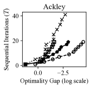
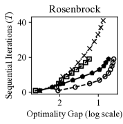
Figure 1: Comparison of the number of sequential iterations $T$ ($y$-axis) required by different methods to achieve the same optimality gap $F({\bm{\theta}})-\inf_{{\bm{\theta}}}F({\bm{\theta}})$ ($x$-axis) for various synthetic functions of $d=10^{5}$ and $\sigma^{2}=0$. The parallelism $N$ is set to 5 and each curve denotes the mean from five independent experiments.

Here we utilize synthetic functions to demonstrate the enhanced performance of our OptEx algorithm compared to existing baselines, including the standard FOO algorithm namely Vanilla baseline, FOO with parallelized line search namely LineSearch baseline where learning rate is scaled by $s\in[N]$ for every parallel process, and FOO with ideally parallelized iterations namely Target baseline which impractically utilizes the ground-truth gradient to obtain the inputs for parallelized iterations. Specifically, the Vanilla baseline is equivalent to Algo. 1 with parallelism of $N\,{=}\,1$; the LineSearch baseline is equivalent to Algo. 1 with ${\bm{\mu}}_{t}({\bm{\theta}}_{t,s-1})$ being $\nabla f({\bm{\theta}}_{t,0},{\bm{x}})$; the Target baseline is equivalent to Algo. 1 with ${\bm{\mu}}_{t}({\bm{\theta}}_{t,s-1})$ being $\nabla f({\bm{\theta}}_{t,s-1},{\bm{x}})$ and ${\bm{\theta}}_{t}={\bm{\theta}}_{t}^{\smash{(N)}}$. These synthetic functions and the experimental setup applied here are in Appx. B.1.

The results, depicted in Fig. 1 with $d=10^{5}$, $\sigma^{2}=0$, and $N=5$, reveal the efficacy of OptEx even for deterministic optimization (i.e., $\sigma^{2}=0$). Specifically, Fig. 1 demonstrates that OptEx consistently achieves a notable speedup, at least 2$\times$ that of Vanilla, when operating with a parallelism of $N=5$ to reach an equivalent level of optimality gap. This observation is in congruence with the result of Cor. 2. Of note, OptEx exhibits slight underperformance compared to Target, which is reasonable since Target can utilize the ground-truth gradient whereas OptEx relies on kernelized gradient estimation for parallelized iterations. This observation is in line with the insight from our iteration complexity analysis detailed in Thm. 2. Overall, the results in Fig. 1 have provided empirical support for the efficacy of our OptEx in expediting FOO, which substantiates our theoretical justifications in Sec. 5.

6.2 Reinforcement Learning

We proceed to compare our OptEx with previously established baselines as introduced in Sec. 6.1, engaging in various reinforcement learning tasks from the OpenAI Gym suite (Brockman et al., 2016), with the deployment of DQN agents (Mnih et al., 2015) where $d=830090$. The parallelism parameter is set at $N=4$. A detailed exposition of the experimental framework is provided in Appx. B.2. The encapsulation of our findings is presented in Fig. 2. As illustrated in Fig. 2, the integration of parallel computing techniques, including LineSearch, Target, and OptEx, demonstrably outperforms the traditional Vanilla method in terms of optimization efficiency. Importantly, amongst these methodologies, OptEx consistently demonstrates a more stable and superior efficiency enhancement across varying reinforcement learning endeavors, hence corroborating the efficacy of OptEx in improving the efficiency of established FOO algorithms.

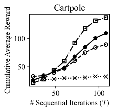
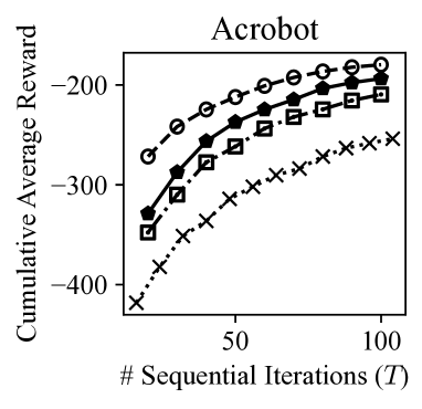
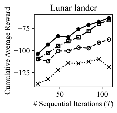
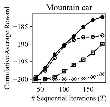
Figure 2: Comparison of the cumulative average reward ($y$-axis) achieved by applying different methods to train DQN on RL tasks when a varying number of sequential episodes $T$ is given ($x$-axis). The parallelism $N$ is set to 4 and each curve denotes the mean from three independent experiments.

6.3 Neural Network Training

Additionally, we examine the efficacy of our OptEx in expediting the optimization of deep neural networks, specifically for image classification and text autoregression tasks.

Image Classification.

We first compare our OptEx with the baselines introduced in Sec. 6.1 for the optimization of a 5-layer MLP model, featuring a complexity of $d=830090$ and a parallelism of $N=4$. This comparison was conducted using two distinct datasets: the MNIST dataset (LeCun et al., 2010) and the fashion MNIST dataset (Xiao et al., 2017). Comprehensive details regarding the experimental setup are provided in Appx. B.3, with the conclusive findings illustrated in Fig. 3. Intriguingly, as evidenced by Fig. 3, OptEx consistently outperforms Vanilla by a large margin in terms of both training and testing errors across the MNIST and fashion MNIST datasets, given an equal number of sequential iterations $T$. Remarkably, the efficiency of OptEx approaches that of the theoretically ideal algorithm Target, which is a notable achievement. In addition, OptEx exhibits enhanced stability compared to Target when $T$ is approximately 35 in Fig. 3. This stability is likely attributable to the reduced gradient estimation error that can be achieved by our innovative kernelized gradient estimation approach, as discussed in Sec. 4.1. Overall, these results emphatically underscore the capability of OptEx in significantly expedite FOO algorithms, even in the context of deep neural network optimization.

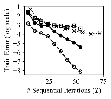
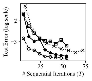
	(a) MNIST
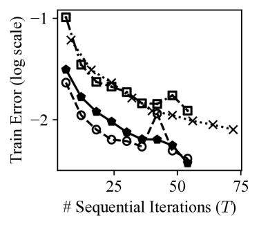
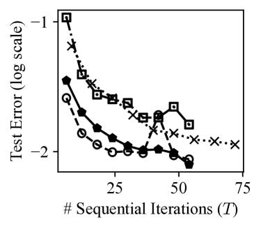
	(b) Fashion MNIST

Figure 3: Comparison of the train (left) and test (right) error (i.e., 1 - accuracy in log scale for $y$-axis) achieved by applying different methods to train MLP on MINIST and fashion MNIST datasets when a varying number of sequential iterations $T$ is given ($x$-axis). The parallelism $N$ is set to 4 and each curve denotes the mean from five independent experiments.

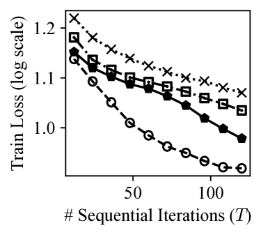
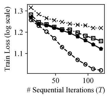
Figure 4: Comparison of the train loss ($y$-axis) achieved by applying different methods to train transformer on the text of “Harry Potter and the Sorcerer’s Stone” (left) and a subset of works of Shakespeare (right) when a varying number of sequential iterations $T$ is given ($x$-axis). The parallelism $N$ is set to 4 and each curve denotes the mean from three independent experiments.

Text Autoregression.

Finally, OptEx is compared against the baselines introduced in Sec.6.1 in optimizing an autoregressive transformer model (Hennigan et al., 2020) with a parameter size of $d\,{=}\,1626496$ and parallelism of $N\,{=}\,4$. We employ two distinct text datasets for this comparison: “Harry Potter and the Sorcerer’s Stone” and a curated collection of works from Shakespeare. The full experimental setting is detailed in Appx. B.3 and the pivotal results are showcased in Fig. 4. Remarkably, despite the complexity and difficulty of these training tasks, OptEx demonstrates a noticeable acceleration over the standard FOO algorithm (Vanilla), which still outperforms the LineSearch baseline. These results therefore again highlight the efficacy of our OptEx in expediting the training of neural networks. However, in these intricate scenarios, OptEx falls short of the theoretically ideal algorithm Target. This underperformance likely stems from the challenges inherent in precise gradient estimation within such complex models, underscoring the imperative for advanced kernel development for our kernelized gradient estimation in deep neural network training.

7 Conclusion

In conclusion, our first-order optimization expedited with approximately parallelized iterations (OptEx) framework emerges as a transformative approach in the realm of FOO, addressing its traditional inefficiencies by enabling parallelized iterations through innovative kernelized gradient estimation. This advancement not only breaks the iterative dependency barrier inherent in FOO, resulting in fewer necessary sequential iterations for convergence, but also provides theoretical underpinnings confirming the efficacy and reliability of the approach. Empirical validations across a spectrum of applications, from synthetic functions to complex neural network training tasks, further attest to the significant efficiency enhancements OptEx brings to computational domains, heralding an interesting direction for FOO.

Statement of the Potential Broader Impact

This paper presents work that aims to leverage parallel computing to expedite established FOO algorithms through approximately parallelized iterations. So, we do not see any potential societal consequences of our work that must be specifically highlighted here.

Appendix A Proofs

A.1 Proof of Proposition 4.1

Recall that we have defined ${\bm{k}}_{t}^{\top}({\bm{\theta}})\triangleq[k({\bm{\theta}},{\bm{\theta}}_{\tau})]_{\tau=1}^{N(t-1)}$, and ${\mathbf{K}}_{t}\triangleq[k({\bm{\theta}}_{\tau},{\bm{\theta}}_{\tau^{\prime}})]_{\tau=\tau^{\prime}=1}^{N(t-1)}$. Let $\otimes$ denote the Kronecker product, by introducing the fact that ${\mathbf{K}}(\cdot,\cdot)=k(\cdot,\cdot)\,{\mathbf{I}}$ into ${\mathbf{V}}_{t}^{\top}({\bm{\theta}})$ and ${\mathbf{U}}_{t}$ from the Gaussian process posterior (3), we have that

$${\mathbf{V}}^{\top}_{t}({\bm{\theta}})=\begin{bmatrix}k({\bm{\theta}},{\bm{\theta}}_{1}){\mathbf{I}}&\cdots&k({\bm{\theta}},{\bm{\theta}}_{\tau}){\mathbf{I}}&\cdots&k({\bm{\theta}},{\bm{\theta}}_{t-1}){\mathbf{I}}\end{bmatrix}={\bm{k}}_{t}^{\top}({\bm{\theta}})\otimes{\mathbf{I}}\ .$$ (9)

Similarly,

$${\mathbf{U}}_{t} =\begin{bmatrix}k({\bm{\theta}}_{1},{\bm{\theta}}_{1}){\mathbf{I}}&\cdots&k({\bm{\theta}}_{1},{\bm{\theta}}_{\tau^{\prime}}){\mathbf{I}}&\cdots&k({\bm{\theta}}_{1},{\bm{\theta}}_{t-1}){\mathbf{I}}\\ \vdots&\vdots&\vdots&\vdots&\vdots\\ k({\bm{\theta}}_{\tau},{\bm{\theta}}_{1}){\mathbf{I}}&\cdots&k({\bm{\theta}}_{\tau},{\bm{\theta}}_{\tau^{\prime}}){\mathbf{I}}&\cdots&k({\bm{\theta}}_{\tau},{\bm{\theta}}_{t-1}){\mathbf{I}}\\ \vdots&\vdots&\vdots&\vdots&\vdots\\ k({\bm{\theta}}_{t-1},{\bm{\theta}}_{1}){\mathbf{I}}&\cdots&k({\bm{\theta}}_{t-1},{\bm{\theta}}_{\tau^{\prime}}){\mathbf{I}}&\cdots&k({\bm{\theta}}_{t-1},{\bm{\theta}}_{t-1}){\mathbf{I}}\end{bmatrix}={\mathbf{K}}_{t}\otimes{\mathbf{I}}\ .$$ (10)

By introducing the results above into the posterior mean and variance in (3), we have

$${\bm{\mu}}_{t}({\bm{\theta}}) \stackrel{{\scriptstyle(a)}}{{=}}{\mathbf{V}}^{\top}_{t}({\bm{\theta}})\left({\mathbf{U}}_{t}+\sigma^{2}{\mathbf{I}}\right)^{-1}\mathrm{vec}({\mathbf{G}}_{t}^{\top})$$ (11)

$$\stackrel{{\scriptstyle(b)}}{{=}}\left({\bm{k}}_{t}^{\top}({\bm{\theta}})\otimes{\mathbf{I}}\right)\left({\mathbf{K}}_{t}\otimes{\mathbf{I}}+\sigma^{2}{\mathbf{I}}\right)^{-1}\mathrm{vec}({\mathbf{G}}_{t}^{\top})$$

$$\stackrel{{\scriptstyle(c)}}{{=}}\left({\bm{k}}_{t}^{\top}({\bm{\theta}})\otimes{\mathbf{I}}\right)\left[\left({\mathbf{K}}_{t}+\sigma^{2}{\mathbf{I}}\right)\otimes{\mathbf{I}}\right]^{-1}\mathrm{vec}({\mathbf{G}}_{t}^{\top})$$

$$\stackrel{{\scriptstyle(d)}}{{=}}\left({\bm{k}}_{t}^{\top}({\bm{\theta}})\otimes{\mathbf{I}}\right)\left[\left({\mathbf{K}}_{t}+\sigma^{2}{\mathbf{I}}\right)^{-1}\otimes{\mathbf{I}}\right]\mathrm{vec}({\mathbf{G}}_{t}^{\top})$$

$$\stackrel{{\scriptstyle(e)}}{{=}}\left(\left[{\bm{k}}_{t}^{\top}({\bm{\theta}})\left({\mathbf{K}}_{t}+\sigma^{2}{\mathbf{I}}\right)^{-1}\right]\otimes{\mathbf{I}}\right)\mathrm{vec}\left({\mathbf{G}}^{\top}_{t}\right)$$

$$\stackrel{{\scriptstyle(f)}}{{=}}\mathrm{vec}\left({\mathbf{G}}_{t}^{\top}\left[{\bm{k}}_{t}^{\top}({\bm{\theta}})\left({\mathbf{K}}_{t}+\sigma^{2}{\mathbf{I}}\right)^{-1}\right]^{\top}\right)$$

$$\stackrel{{\scriptstyle(g)}}{{=}}\left[\left({\bm{k}}_{t}^{\top}({\bm{\theta}})\left({\mathbf{K}}_{t}+\sigma^{2}{\mathbf{I}}\right)^{-1}\right){\mathbf{G}}_{t}\right]^{\top}$$

where $(c)$ come from the bi-linearity of the Kronecker product, i.e., $({\mathbf{A}}+{\mathbf{B}})\otimes{\mathbf{C}}={\mathbf{A}}\otimes{\mathbf{C}}+{\mathbf{B}}\otimes{\mathbf{C}}$ while $(d)$ is from the inverse of the Kronecker product, i.e., $\left({\mathbf{A}}\otimes{\mathbf{B}}\right)^{-1}={\mathbf{A}}^{-1}\otimes{\mathbf{B}}^{-1}$. In addition, $(e)$ is due to the mixed-product property of the Kronecker product, i.e., $({\mathbf{A}}\otimes{\mathbf{B}})({\mathbf{C}}\otimes{\mathbf{D}})=({\mathbf{A}}{\mathbf{C}})\otimes({\mathbf{B}}{\mathbf{D}})$, and $(f)$ results from the mixed Kronecker matrix-vector product of the Kronecker product, i.e., $({\mathbf{A}}\otimes{\mathbf{B}})\mathrm{vec}({\mathbf{C}})=\mathrm{vec}({\mathbf{B}}{\mathbf{C}}{\mathbf{A}}^{\top})$.

Similarly,

$${\bm{\Sigma}}_{t}^{2}({\bm{\theta}},{\bm{\theta}}^{\prime}) \stackrel{{\scriptstyle(a)}}{{=}}{\mathbf{K}}\left({\bm{\theta}},{\bm{\theta}}^{\prime}\right)-{\mathbf{V}}^{\top}_{t}({\bm{\theta}})\left({\mathbf{U}}_{t}+\sigma^{2}{\mathbf{I}}\right)^{-1}{\mathbf{\Phi}}_{n}\left({\bm{\theta}}^{\prime}\right)$$ (12)

$$\stackrel{{\scriptstyle(b)}}{{=}}k({\bm{\theta}},{\bm{\theta}}^{\prime}){\mathbf{I}}-\left(\left[{\bm{k}}_{t}^{\top}({\bm{\theta}})\left({\mathbf{K}}_{t}+\sigma^{2}{\mathbf{I}}\right)^{-1}\right]\otimes{\mathbf{I}}\right)\left({\bm{k}}_{t}({\bm{\theta}}^{\prime})\otimes{\mathbf{I}}\right)$$

$$\stackrel{{\scriptstyle(c)}}{{=}}k({\bm{\theta}},{\bm{\theta}}^{\prime}){\mathbf{I}}-\left({\bm{k}}_{t}^{\top}({\bm{\theta}})\left({\mathbf{K}}_{t}+\sigma^{2}{\mathbf{I}}\right)^{-1}{\bm{k}}_{t}({\bm{\theta}}^{\prime})\right){\mathbf{I}}$$

$$\stackrel{{\scriptstyle(d)}}{{=}}\left(k({\bm{\theta}},{\bm{\theta}}^{\prime})-{\bm{k}}_{t}^{\top}({\bm{\theta}})\left({\mathbf{K}}_{t}+\sigma^{2}{\mathbf{I}}\right)^{-1}{\bm{k}}_{t}({\bm{\theta}}^{\prime})\right){\mathbf{I}}$$

where $(b)$ comes from the result in (11), $(c)$ results from the mixed-product property of the Kronecker product and the fact that $\left({\bm{k}}_{t}^{\top}({\bm{\theta}})\left({\mathbf{K}}_{t}+\sigma^{2}{\mathbf{I}}\right)^{-1}{\bm{k}}_{t}({\bm{\theta}}^{\prime})\right)$ is a scalar. This finally concludes our proof.

A.2 Proof of Theorem 1

To begin with, we introduce the following lemmas:

Lemma A.1 ((Laurent and Massart, 2000)).

Let ${\bm{\zeta}}\sim{\mathcal{N}}({\bm{0}},{\mathbf{I}}_{d})$ and $\delta\in(0,1)$ then

$${\mathbb{P}}\left(\left\|{\bm{\zeta}}\right\|_{2}\leq\sqrt{d+2(\sqrt{d}+1)\ln(1/\delta)}\right)\geq 1-\delta\ .$$ (13)

Lemma A.2 (Lemma 2 in Appx. B of (Chowdhury & Gopalan, 2021)).

For any $\sigma\in{\mathbb{R}}$ and any matrix ${\mathbf{A}}$, the following hold

$${\mathbf{I}}-{\mathbf{A}}^{\top}\left({\mathbf{A}}{\mathbf{A}}^{\top}+\sigma^{2}{\mathbf{I}}\right)^{-1}{\mathbf{A}} =\sigma^{2}\left({\mathbf{A}}^{\top}{\mathbf{A}}+\sigma^{2}{\mathbf{I}}\right)^{-1}\ .$$ (14)

Lemma A.3 (Sherman-Morrison formula).

For any invertible square matrix ${\mathbf{A}}$ and column vectors ${\bm{u}},{\bm{v}}$, suppose ${\mathbf{A}}+{\bm{u}}{\bm{v}}^{\top}$ is invertible, then the following holds

$$\left({\mathbf{A}}+{\bm{u}}{\bm{v}}^{\top}\right)^{-1}={\mathbf{A}}^{-1}-\frac{{\mathbf{A}}^{-1}{\bm{u}}{\bm{v}}^{\top}{\mathbf{A}}^{-1}}{1+{\bm{v}}^{\top}{\mathbf{A}}^{-1}{\bm{u}}}\ .$$ (15)

Lemma A.4 (Non-Increasing Variance Norm).

Define variance ${\bm{\Sigma}}_{n}^{2}({\bm{\theta}})\triangleq{\bm{\Sigma}}_{n-1}^{2}({\bm{\theta}},{\bm{\theta}})$ with $n$ being the number of gradients employed to evaluate the mean and covariance in Prop. 4.1. Then for any ${\bm{\theta}}\in{\mathbb{R}}^{d}$ and $n\geq 1$,

$$\left\|{\bm{\Sigma}}_{n}^{2}({\bm{\theta}})\right\|\leq\left\|{\bm{\Sigma}}_{n-1}^{2}({\bm{\theta}})\right\|\ .$$ (16)

Proof.

We follow the idea in (Chowdhury & Gopalan, 2021) and (Shu et al., 2023a) to prove it. Specifically, we firstly define $k({\bm{\theta}},{\bm{\theta}}^{\prime})=\phi({\bm{\theta}})^{\top}\phi({\bm{\theta}}^{\prime})$ and ${\bm{\phi}}_{n}\triangleq[\phi({\bm{\theta}}_{i})]_{i=1}^{n}$. Then the matrix ${\mathbf{K}}_{n}$ in Prop. 4.1 can be reformulated as

$${\mathbf{K}}_{n}={\bm{\phi}}_{n}^{\top}{\bm{\phi}}_{n}\ ,$$ (17)

and based on the definition of ${\mathbf{\Phi}}_{n}\triangleq{\bm{\phi}}_{n}{\bm{\phi}}_{n}^{\top}+\sigma^{2}{\mathbf{I}}$,

$${\bm{\Sigma}}_{t}^{2}({\bm{\theta}}) \stackrel{{\scriptstyle(a)}}{{=}}\left(\phi({\bm{\theta}})^{\top}\phi({\bm{\theta}})-\phi({\bm{\theta}})^{\top}{\bm{\phi}}_{n}\left({\bm{\phi}}_{n}^{\top}{\bm{\phi}}_{n}+\sigma^{2}{\mathbf{I}}\right)^{-1}{\bm{\phi}}_{n}^{\top}\phi({\bm{\theta}})\right)\,{\mathbf{I}}$$ (18)

$$\stackrel{{\scriptstyle(b)}}{{=}}\left(\phi({\bm{\theta}})^{\top}\left({\mathbf{I}}-{\bm{\phi}}_{n}\left({\bm{\phi}}_{n}^{\top}{\bm{\phi}}_{n}+\sigma^{2}{\mathbf{I}}\right)^{-1}{\bm{\phi}}_{n}^{\top}\right)\phi({\bm{\theta}})\right)\,{\mathbf{I}}$$

$$\stackrel{{\scriptstyle(c)}}{{=}}\left(\sigma^{2}\phi({\bm{\theta}})^{\top}\left({\bm{\phi}}_{n}{\bm{\phi}}_{n}^{\top}+\sigma^{2}{\mathbf{I}}\right)^{-1}\phi({\bm{\theta}})\right)\,{\mathbf{I}}$$

$$\stackrel{{\scriptstyle(d)}}{{=}}\left(\sigma^{2}\phi({\bm{\theta}})^{\top}{\mathbf{\Phi}}_{n}^{-1}\phi({\bm{\theta}})\right)\,{\mathbf{I}}$$

where $(c)$ comes from Lemma A.2 by replacing the matrix ${\mathbf{A}}$ in Lemma A.2 with the matrix ${\bm{\phi}}_{n}^{\top}$.

As a result,

$${\bm{\Sigma}}_{n}^{2}({\bm{\theta}}) \stackrel{{\scriptstyle(a)}}{{=}}\left(\sigma^{2}\phi({\bm{\theta}})^{\top}{\mathbf{\Phi}}_{n}^{-1}\phi({\bm{\theta}})\right)\,{\mathbf{I}}$$ (19)

$$\stackrel{{\scriptstyle(b)}}{{=}}\left(\sigma^{2}\phi({\bm{\theta}})^{\top}\left({\bm{\phi}}_{n-1}{\bm{\phi}}_{n-1}^{\top}+\sigma^{2}{\mathbf{I}}+\phi({\bm{\theta}}_{n})\phi({\bm{\theta}}_{n})^{\top}\right)^{-1}\phi({\bm{\theta}})\right)\,{\mathbf{I}}$$

$$\stackrel{{\scriptstyle(c)}}{{=}}\left(\sigma^{2}\phi({\bm{\theta}})^{\top}\left({\mathbf{\Phi}}_{n-1}+\phi({\bm{\theta}}_{n})\phi({\bm{\theta}}_{n})^{\top}\right)^{-1}\phi({\bm{\theta}})\right)\,{\mathbf{I}}$$

$$\stackrel{{\scriptstyle(d)}}{{=}}\left(\sigma^{2}\phi({\bm{\theta}})^{\top}{\mathbf{\Phi}}_{n-1}^{-1}\phi({\bm{\theta}})-\sigma^{2}\left(1+\phi({\bm{\theta}}_{n})^{\top}{\mathbf{\Phi}}_{n-1}^{-1}\phi({\bm{\theta}}_{n})\right)^{-1}\phi({\bm{\theta}})^{\top}{\mathbf{\Phi}}_{n-1}^{-1}\phi({\bm{\theta}}_{n})\phi({\bm{\theta}}_{n})^{\top}{\mathbf{\Phi}}_{n-1}^{-1}\phi({\bm{\theta}})\right)\,{\mathbf{I}}$$

$$\stackrel{{\scriptstyle(e)}}{{=}}{\bm{\Sigma}}_{n-1}^{2}({\bm{\theta}})-\sigma^{2}\left(1+\phi({\bm{\theta}}_{n})^{\top}{\mathbf{\Phi}}_{n-1}^{-1}\phi({\bm{\theta}}_{n})\right)^{-1}\phi({\bm{\theta}})^{\top}{\mathbf{\Phi}}_{n-1}^{-1}\phi({\bm{\theta}}_{n})\phi({\bm{\theta}}_{n})^{\top}{\mathbf{\Phi}}_{n-1}^{-1}\phi({\bm{\theta}})\,{\mathbf{I}}$$

$$\stackrel{{\scriptstyle(f)}}{{\preccurlyeq}}{\bm{\Sigma}}_{n-1}^{2}({\bm{\theta}})$$

where $(b)$ is due to the fact that ${\mathbf{\Phi}}_{n}{\mathbf{\Phi}}_{n}^{\top}={\mathbf{\Phi}}_{n-1}{\mathbf{\Phi}}_{n-1}^{\top}+\phi({\bm{\theta}}_{n})\phi({\bm{\theta}}_{n})^{\top}$, and $(d)$ is from Lemma A.3. Finally, $(f)$ derives from the positive semi-definite property of ${\mathbf{\Phi}}_{n-1}^{-1}\phi({\bm{\theta}}_{t})\phi({\bm{\theta}}_{t})^{\top}{\mathbf{\Phi}}_{n-1}^{-1}$ and ${\mathbf{\Phi}}_{n-1}^{-1}$, leading to the conclusion of our proof. ∎

Lemma A.5 (lower Bound of Variance Norm).

Following the definition in Lemma A.4, for any ${\bm{\theta}}\in{\mathbb{R}}^{d}$ and $n\geq 1$,

$$\left\|{\bm{\Sigma}}_{n}^{2}({\bm{\theta}})\right\|\geq\frac{1}{(\kappa+1/\sigma^{2})}\left\|{\bm{\Sigma}}_{n-1}^{2}({\bm{\theta}})\right\|\ .$$ (20)

Proof.

Again, we follow the idea in (Chowdhury & Gopalan, 2021) and (Shu et al., 2023a) to prove it. we first prove the following inequality

$$\left\|{\mathbf{\Phi}}^{-1/2}_{n-1}\phi({\bm{\theta}}_{n})\phi({\bm{\theta}}_{n})^{\top}{\mathbf{\Phi}}^{-1/2}_{n-1}\right\| \stackrel{{\scriptstyle(a)}}{{=}}\left\|\phi({\bm{\theta}}_{n})^{\top}{\mathbf{\Phi}}^{-1/2}_{n-1}\right\|^{2}$$ (21)

$$\stackrel{{\scriptstyle(b)}}{{=}}\phi({\bm{\theta}}_{n})^{\top}{\mathbf{\Phi}}^{-1}_{n-1}\phi({\bm{\theta}}_{n})$$

$$\stackrel{{\scriptstyle(c)}}{{\leq}}\phi({\bm{\theta}}_{n})^{\top}{\mathbf{\Phi}}^{-1}_{n-2}\phi({\bm{\theta}}_{n})$$

$$\stackrel{{\scriptstyle(d)}}{{\leq}}\sigma^{2}\phi({\bm{\theta}}_{n})^{\top}\phi({\bm{\theta}}_{n})$$

$$\stackrel{{\scriptstyle(e)}}{{\leq}}\kappa\sigma^{2}$$

where $(c)$ comes from the fact that ${\mathbf{\Phi}}_{n-1}={\mathbf{\Phi}}^{-1}_{n-2}+\phi({\bm{\theta}}_{n-1}\phi({\bm{\theta}}_{n-1})^{\top}\succcurlyeq{\mathbf{\Phi}}_{n-2}\succcurlyeq\cdots\succcurlyeq\sigma^{2}{\mathbf{I}}$ and $(e)$ is due to the fact that $\phi({\bm{\theta}}_{n})^{\top}\phi({\bm{\theta}}_{n})=k({\bm{\theta}}_{n},{\bm{\theta}}_{n})\leq\kappa$.

Then, based on the reformulation of ${\bm{\Sigma}}_{n}^{2}({\bm{\theta}})$ in (19), we have that

$${\bm{\Sigma}}_{n}^{2}({\bm{\theta}}) \stackrel{{\scriptstyle(a)}}{{=}}\left(\sigma^{2}\phi({\bm{\theta}})^{\top}\left({\mathbf{\Phi}}_{n-1}+\phi({\bm{\theta}}_{n})\phi({\bm{\theta}}_{n})^{\top}\right)^{-1}\phi({\bm{\theta}})\right)\,{\mathbf{I}}$$ (22)

$$\stackrel{{\scriptstyle(b)}}{{=}}\left(\sigma^{2}\phi({\bm{\theta}})^{\top}{\mathbf{\Phi}}^{-1/2}_{n-1}\left({\mathbf{I}}+{\mathbf{\Phi}}^{-1/2}_{n-1}\phi({\bm{\theta}}_{n})\phi({\bm{\theta}}_{n})^{\top}{\mathbf{\Phi}}^{-1/2}_{n-1}\right)^{-1}{\mathbf{\Phi}}^{-1/2}_{n-1}\phi({\bm{\theta}})\right)\,{\mathbf{I}}$$

$$\stackrel{{\scriptstyle(c)}}{{\succcurlyeq}}\frac{\sigma^{2}}{1+\kappa\sigma^{2}}\phi({\bm{\theta}})^{\top}{\mathbf{\Phi}}^{-1}_{n-1}\phi({\bm{\theta}})\,{\mathbf{I}}$$

$$\stackrel{{\scriptstyle(d)}}{{=}}\frac{\sigma^{2}}{1+\kappa\sigma^{2}}{\bm{\Sigma}}_{n-1}^{2}({\bm{\theta}})$$

where $(c)$ comes from (21). This finally concludes our proof. ∎

Lemma A.6 (Information Gain).

Define ${\mathbf{G}}_{n}\triangleq\left[\nabla f({\bm{x}},{\bm{\theta}}_{i})\right]_{i=1}^{n}$, $\bm{\nabla}_{n}\triangleq\left[\nabla F({\bm{\theta}}_{i})\right]_{i=1}^{n}$, and ${\mathbf{K}}_{n}\triangleq\left[k({\bm{\theta}}_{i},{\bm{\theta}}_{j})\right]_{i,j=1}^{n}$. The information gain $I(\mathrm{vec}({\mathbf{G}}_{n});\mathrm{vec}(\bm{\nabla}_{n}))$ has the following form with Assump. 1, 2:

$$I(\mathrm{vec}({\mathbf{G}}_{n});\mathrm{vec}(\bm{\nabla}_{n}))=\frac{d}{2}\ln\left(\det({\mathbf{I}}+\sigma^{-2}{\mathbf{K}}_{n})\right)\ .$$ (23)

Proof.

Based on our Assump. 1, 2, the following holds respectively:

$$\mathrm{vec}({\mathbf{G}}_{n})\mid\mathrm{vec}(\bm{\nabla}_{n})\sim{\mathcal{N}}({\bm{0}},\sigma^{2}\,{\mathbf{I}}_{nd})\,,\ \text{and}\ \ \mathrm{vec}({\mathbf{G}}_{n})\sim\mathcal{GP}\left({\bm{0}},\left({\mathbf{K}}_{n}+\sigma^{2}{\mathbf{I}}_{n}\right)\otimes{\mathbf{I}}_{d}\right)\ .$$ (24)

Due to the fact that $H({\textnormal{z}})=\frac{1}{2}\ln(\det(2\pi e{\bm{\Sigma}}))$ if ${\textnormal{z}}\sim{\mathcal{N}}(\mu,{\bm{\Sigma}})$, the following holds

$$I(\mathrm{vec}({\mathbf{G}}_{n});\mathrm{vec}(\bm{\nabla}_{n})) \stackrel{{\scriptstyle(a)}}{{=}}H(\mathrm{vec}({\mathbf{G}}_{n}))-H(\mathrm{vec}({\mathbf{G}}_{n})\mid\mathrm{vec}(\bm{\nabla}_{n}))$$ (25)

$$\stackrel{{\scriptstyle(b)}}{{=}}\frac{1}{2}\ln\left(\det\left(2\pi e\left({\mathbf{K}}_{n}+\sigma^{2}{\mathbf{I}}_{n}\right)\otimes{\mathbf{I}}_{d}\right)\right)-\frac{1}{2}\ln\left(\det\left(2\pi e\sigma^{2}{\mathbf{I}}_{nd}\right)\right)$$

$$\stackrel{{\scriptstyle(c)}}{{=}}\frac{1}{2}\ln\left(\left[\det\left(2\pi e\left({\mathbf{K}}_{n}+\sigma^{2}{\mathbf{I}}_{n}\right)\right)\right]^{d}\left(\det\left({\mathbf{I}}_{d}\right)\right)^{n}\right)-\frac{1}{2}\ln\left(\det\left(2\pi e\sigma^{2}{\mathbf{I}}_{nd}\right)\right)$$

$$\stackrel{{\scriptstyle(d)}}{{=}}\frac{1}{2}\ln\left(\frac{\det(2\pi e({\mathbf{K}}_{n}+\sigma^{2}{\mathbf{I}}_{n}))}{\det(2\pi e\sigma^{2}{\mathbf{I}}_{n})}\right)^{d}$$

$$\stackrel{{\scriptstyle(e)}}{{=}}\frac{d}{2}\ln\left(\det({\mathbf{I}}+\sigma^{-2}{\mathbf{K}}_{n})\right)$$

where $(a)$ comes from the definition of information gain, $(b)$ derives from the results in (24), and $(c)$ is due to the fact that $\det({\mathbf{A}}\otimes{\mathbf{B}})=\left(\det({\mathbf{A}})\right)^{b}\left(\det({\mathbf{B}})\right)^{a}$ given the $a\times a$-dimensional matrix ${\mathbf{A}}$ and $b\times b$-dimensional matrix ${\mathbf{B}}$. In addition, $(e)$ follows from $\det({\mathbf{A}}{\mathbf{B}}^{-1})=\det({\mathbf{A}})/\det({\mathbf{B}})$. This then concludes our proof. ∎

Lemma A.7 (Sum of Variance).

Define the maximal information gain

$$\gamma_{n}\triangleq\max_{\{{\bm{\theta}}_{j}\}_{j=1}^{n}\subset{\mathbb{R}}^{d}}I(\mathrm{vec}({\mathbf{G}}_{n});\mathrm{vec}(\bm{\nabla}_{n}))\ ,$$ (26)

the following then holds

$$\frac{1}{n}\sum_{i=0}^{n-1}\left\|{\bm{\Sigma}}_{i}^{2}({\bm{\theta}})\right\|\leq\frac{2\sigma^{2}\gamma_{n}}{d}\ .$$ (27)

Proof.

To begin with, we show the following inequalities resulting from the matrix determinant lemma:

$$\det\left({\mathbf{\Phi}}_{i+1}\right) =\det\left({\mathbf{\Phi}}_{i}+\phi({\bm{\theta}})\phi({\bm{\theta}})^{\top}\right)$$ (28)

$$=\det\left({\mathbf{\Phi}}_{i}\right)\left(1+\phi({\bm{\theta}})^{\top}{\mathbf{\Phi}}_{i}^{-1}\phi({\bm{\theta}})\right)\ .$$

Given $\kappa\leq\sigma^{2}$, since $\left\|{\bm{\Sigma}}^{2}_{n}({\bm{\theta}})\right\|\leq\left\|{\bm{\Sigma}}^{2}_{n-1}({\bm{\theta}})\right\|\leq\cdots\leq\left\|{\bm{\Sigma}}^{2}_{0}({\bm{\theta}})\right\|=|k({\bm{\theta}},{\bm{\theta}})|\leq\kappa$ from Lemma A.4, we then have $\phi({\bm{\theta}})^{\top}{\mathbf{\Phi}}_{i}^{-1}\phi({\bm{\theta}})\leq 1$. As a result,

$$\frac{1}{2}\sum_{i=0}^{n-1}\left\|{\bm{\Sigma}}_{i}^{2}({\bm{\theta}})\right\| \stackrel{{\scriptstyle(a)}}{{=}}\sum_{i=0}^{n-1}\frac{1}{2}\sigma^{2}\phi({\bm{\theta}})^{\top}{\mathbf{\Phi}}_{i}^{-1}\phi({\bm{\theta}})$$ (29)

$$\stackrel{{\scriptstyle(b)}}{{\leq}}\sum_{i=0}^{n-1}\sigma^{2}\ln\left(1+\phi({\bm{\theta}})^{\top}{\mathbf{\Phi}}_{i}^{-1}\phi({\bm{\theta}})\right)$$

$$\stackrel{{\scriptstyle(c)}}{{=}}\sigma^{2}\sum_{i=0}^{n-1}\ln\left(\frac{\det({\mathbf{\Phi}}_{i+1})}{\det({\mathbf{\Phi}}_{i})}\right)$$

$$\stackrel{{\scriptstyle(d)}}{{=}}\sigma^{2}\ln\left(\frac{\det({\mathbf{\Phi}}_{n})}{\det({\mathbf{\Phi}}_{0})}\right)$$

$$\stackrel{{\scriptstyle(e)}}{{=}}\sigma^{2}\ln\left(\frac{\det({\bm{\phi}}_{n}{\bm{\phi}}_{n}^{\top}+\sigma^{2}{\mathbf{I}})}{\det(\sigma^{2}{\mathbf{I}})}\right)$$

$$\stackrel{{\scriptstyle(f)}}{{=}}\sigma^{2}\ln\left(\det(\sigma^{-2}{\bm{\phi}}_{n}{\bm{\phi}}_{n}^{\top}+{\mathbf{I}})\right)$$

$$\stackrel{{\scriptstyle(g)}}{{=}}\sigma^{2}\ln\left(\det({\mathbf{I}}+\sigma^{-2}{\bm{\phi}}_{n}^{\top}{\bm{\phi}}_{n})\right)$$

$$\stackrel{{\scriptstyle(h)}}{{\leq}}\frac{2\sigma^{2}\gamma_{n}}{d}$$

where $(a)$ follows from the reformulation of ${\bm{\Sigma}}^{2}_{i}({\bm{\theta}})$ in (18), $(b)$ results from the fact that $x/2\leq\ln(1+x)$ for any $x\in(0,1)$, $(c)$ derives from (28), $(d)$ is from the telescoping sum, $(e)$ is due to the fact that $\det({\mathbf{\Phi}}_{0})=\det(\sigma^{2}{\mathbf{I}})$, $(f)$ is from the fact that $\det({\mathbf{A}}{\mathbf{B}}^{-1})=\det({\mathbf{A}})/\det({\mathbf{B}})$, $(g)$ comes from the Sylvester’s determinant identity, i.e., $\det({\mathbf{\Phi}}_{i})=\det({\mathbf{K}}_{i}+\sigma^{2}{\mathbf{I}}_{i})$ according to the definition of ${\mathbf{\Phi}}_{i}$, and $(h)$ results from the fact that ${\mathbf{K}}_{n}={\bm{\phi}}_{n}^{\top}{\bm{\phi}}_{n}$ in (17), the conclusion in Lemma A.6, and the definition of $\gamma_{n}$.

Following the same idea, given $\kappa>\sigma^{2}$, we have

$$\frac{1}{2\kappa}\sum_{i=0}^{n-1}\left\|{\bm{\Sigma}}_{i}^{2}({\bm{\theta}})\right\| \stackrel{{\scriptstyle(a)}}{{=}}\sum_{i=0}^{n-1}\frac{\sigma^{2}}{2\kappa}\phi({\bm{\theta}})^{\top}{\mathbf{\Phi}}_{i}^{-1}\phi({\bm{\theta}})$$ (30)

$$\stackrel{{\scriptstyle(b)}}{{\leq}}\sum_{i=0}^{n-1}\ln\left(1+\frac{\sigma^{2}}{\kappa}\phi({\bm{\theta}})^{\top}{\mathbf{\Phi}}_{i}^{-1}\phi({\bm{\theta}})\right)$$

$$\stackrel{{\scriptstyle(c)}}{{\leq}}\sum_{i=0}^{n-1}\ln\left(1+\phi({\bm{\theta}})^{\top}{\mathbf{\Phi}}_{i}^{-1}\phi({\bm{\theta}})\right)$$

$$\stackrel{{\scriptstyle(d)}}{{\leq}}\frac{2\gamma_{n}}{d}\ .$$

Combining the results in (29) and (30), we conclude our proof by

$$\frac{1}{n}\sum_{i=0}^{n-1}\left\|{\bm{\Sigma}}_{i}^{2}({\bm{\theta}})\right\|\leq\frac{4\max\{\kappa,\sigma^{2}\}\gamma_{n}}{d\,n}\ .$$ (31)

∎

Proof of our Thm. 1. Since ${\bm{\Sigma}}_{n}^{-1}({\bm{\theta}})\left[{\bm{\mu}}_{n}({\bm{\theta}})-\nabla F({\bm{\theta}})\right]\sim{\mathcal{N}}({\bm{0}},{\mathbf{I}}_{d})$, according to Lemma A.1, for any $\delta\in(0,1)$ and $\alpha\triangleq d+2(\sqrt{d}+1)\ln(1/\delta)$, with a probability of at least $1-\delta$,

$$\left\|\nabla F({\bm{\theta}})-{\bm{\mu}}_{n}({\bm{\theta}})\right\| \stackrel{{\scriptstyle(a)}}{{\leq}}\left\|{\bm{\Sigma}}_{n}({\bm{\theta}})\right\|\left\|{\bm{\Sigma}}_{n}^{-1}({\bm{\theta}})\left[{\bm{\mu}}_{n}({\bm{\theta}})-\nabla F({\bm{\theta}})\right]\right\|$$ (32)

$$\stackrel{{\scriptstyle(b)}}{{\leq}}\sqrt{\alpha}\left\|{\bm{\Sigma}}^{2}_{n}({\bm{\theta}})\right\|^{1/2}$$

where $(a)$ is from Cauchy–Schwarz inequality and $(b)$ is from Lemma A.1. By introducing the results in Lemma A.5 and Lemma A.7 into the result above and letting $T_{0}=n+1$, we conclude our proof.

A.3 Proof of Theorem 2

In general, we follow the idea in (Liu et al., 2023) to give a high probability convergence for our OptEx algorithm. To begin with, we introduce the following definition and lemma.

Definition A.1 (Sub-Gaussian Random Variable).

A random variable X is $\sigma$-sub-Gaussian if $\mathbb{E}\left[\exp\left(\lambda^{2}{\textnormal{X}}^{2}\right)\right]\leq\exp\left(\lambda^{2}\sigma^{2}\right)\forall\lambda$ such that $|\lambda|\leq\frac{1}{\sigma}$.

Lemma A.8 (Bound for Sub-Gaussian Random Variable).

Suppose X is a $\sigma$-sub-Gaussian random variable, then for any $a\in{\mathbb{R}},0\leq b\leq\frac{1}{2\sigma}$,

$$\mathbb{E}\left[\exp\left(a{\textnormal{X}}+b^{2}{\textnormal{X}}^{2}\right)\right]\leq\exp\left((a^{2}+b^{2})\sigma^{2}+\frac{1}{4}\right)\ .$$ (33)

Proof.

$$\mathbb{E}\left[\exp\left(a{\textnormal{X}}+b^{2}{\textnormal{X}}^{2}\right)\right] \stackrel{{\scriptstyle(a)}}{{\leq}}\mathbb{E}\left[\exp\left(a^{2}\sigma^{2}+\frac{{\textnormal{X}}^{2}}{4\sigma^{2}}+b^{2}{\textnormal{X}}^{2}\right)\right]$$ (34)

$$\stackrel{{\scriptstyle(b)}}{{=}}\exp\left(a^{2}\sigma^{2}\right)\mathbb{E}\left[\exp\left(\left(\frac{1}{4\sigma^{2}}+b^{2}\right){\textnormal{X}}^{2}\right)\right]$$

$$\stackrel{{\scriptstyle(c)}}{{\leq}}\exp\left(a^{2}\sigma^{2}\right)\exp\left(\left(\frac{1}{4\sigma^{2}}+b^{2}\right)\sigma^{2}\right)$$

$$\stackrel{{\scriptstyle(d)}}{{=}}\exp\left((a^{2}+b^{2})\sigma^{2}+\frac{1}{4}\right)$$

where $(c)$ comes from the definition of $\sigma$-sub-Gaussian random variable. ∎

Proof of Thm. 2. Define

$$\sigma^{2}({\bm{\theta}}_{t,s})\triangleq\begin{cases}\left\|{\bm{\Sigma}}^{2}({\bm{\theta}}_{t,s},{\bm{\theta}}_{t,s})\right\|&\text{if }s<N-1\\ \qquad\quad\sigma^{2}&\text{if }s=N-1\ ,\end{cases}\qquad\bm{\varepsilon}({\bm{\theta}}_{t,s})\triangleq\begin{cases}\nabla F({\bm{\theta}}_{t,s})-\nabla{\bm{\mu}}_{t}({\bm{\theta}}_{t,s},{\bm{x}})&\text{if }s<N-1\\ \nabla F({\bm{\theta}}_{t,s})-\nabla f({\bm{\theta}}_{t,s},{\bm{x}})&\text{if }s=N-1\ ,\end{cases}$$ (35)

and

$${\textnormal{X}}_{t,s}\triangleq w\left(\eta(1-\eta L)\nabla F({\bm{\theta}}_{t,s-1})^{\top}\bm{\varepsilon}_{t}({\bm{\theta}}_{t,s-1})+\frac{\eta^{2}L}{2}\left\|\bm{\varepsilon}_{t}({\bm{\theta}}_{t,s-1})\right\|^{2}\right)-w^{2}\eta^{2}(1-\eta L)^{2}\left\|\nabla F({\bm{\theta}}_{t,s-1})\right\|^{2}\sigma^{2}({\bm{\theta}}_{t,s-1})\ .$$ (36)

According to our Lemma A.8 and the fact that each dimension of $\bm{\varepsilon}_{t}({\bm{\theta}}_{t,s})$ follows an independent Gaussian distribution given Assump. 2, the following holds

$$\mathbb{E}\left[\exp\left(\sum_{t=1}^{T}\sum_{s=1}^{N}{\textnormal{X}}_{t,s}\right)\right] \leq\exp\left(\sum_{t=1}^{T}\sum_{s=1}^{N}\left(w^{2}\eta^{2}(1-\eta L)^{2}\left\|\nabla F({\bm{\theta}}_{t,s-1})\right\|^{2}+\frac{w\eta^{2}L}{2}\right)\sigma^{2}({\bm{\theta}}_{t,s-1})\right.$$ (37)

$$\qquad\qquad\qquad\qquad\left.-\sum_{t=1}^{T}\sum_{s=1}^{N}w^{2}\eta^{2}(1-\eta L)^{2}\left\|\nabla F({\bm{\theta}}_{t,s-1})\right\|^{2}\sigma^{2}({\bm{\theta}}_{t,s-1})+\frac{1}{4}\right)$$

$$=\exp\left(\sum_{t=1}^{T}\sum_{s=1}^{N}\frac{w\eta^{2}L}{2}\sigma^{2}({\bm{\theta}}_{t,s-1})+\frac{1}{4}\right)\ .$$

Based on Markov inequality, we have that

$${\mathbb{P}}\left[\exp\left(\sum_{t=1}^{T}\sum_{s=1}^{N}{\textnormal{X}}_{t,s}\right)>\frac{1}{2\delta}\exp\left(\sum_{t=1}^{T}\sum_{s=1}^{N}\frac{w\eta^{2}L}{2}\sigma^{2}({\bm{\theta}}_{t,s-1})\right)\right]\leq\frac{\mathbb{E}\left[\exp\left(\sum_{t=1}^{T}\sum_{s=1}^{N}{\textnormal{X}}_{t,s}\right)\right]}{\exp\left(\sum_{t=1}^{T}\sum_{s=1}^{N}w\eta^{2}L\sigma^{2}({\bm{\theta}}_{t,s-1})/2\right)/(2\delta)}\leq\delta\ .$$ (38)

Therefore, with a probability of at least $1-\delta$,

$$\sum_{t=1}^{T}\sum_{s=1}^{N}{\textnormal{X}}_{t,s}\leq\sum_{t=1}^{T}\sum_{s=1}^{N}\frac{w\eta^{2}L}{2}\sigma^{2}({\bm{\theta}}_{t,s-1})+\ln\left(\frac{1}{2\delta}\right)\ ,$$ (39)

which leads to the following inequality with $w=w$

$$\sum_{t=1}^{T}\sum_{s=1}^{N}\left(\eta(1-\eta L)\nabla F({\bm{\theta}}_{t,s-1})^{\top}\bm{\varepsilon}_{t}({\bm{\theta}}_{t,s-1})+\frac{\eta^{2}L}{2}\left\|\bm{\varepsilon}_{t}({\bm{\theta}}_{t,s-1})\right\|^{2}\right)\leq$$ (40)

$$\qquad\qquad\qquad\sum_{t=1}^{T}\sum_{s=1}^{N}\left(w\eta^{2}(1-\eta L)^{2}\left\|\nabla F({\bm{\theta}}_{t,s-1})\right\|^{2}\sigma^{2}({\bm{\theta}}_{t,s-1})+\frac{\eta^{2}L}{2}\sigma^{2}({\bm{\theta}}_{t,s-1})\right)+\frac{1}{w}\ln\left(\frac{1}{2\delta}\right)\ .$$

Of note, for every proxy step based on SGD:

$$F({\bm{\theta}}_{t,s}) \stackrel{{\scriptstyle(a)}}{{\leq}}F({\bm{\theta}}_{t,s-1})+\nabla F({\bm{\theta}}_{t,s-1})^{\top}({\bm{\theta}}_{t,s}-{\bm{\theta}}_{t,s-1})+\frac{L}{2}\left\|{\bm{\theta}}_{t,s}-{\bm{\theta}}_{t,s-1}\right\|^{2}$$ (41)

$$\stackrel{{\scriptstyle(b)}}{{=}}F({\bm{\theta}}_{t,s-1})-\eta\nabla F({\bm{\theta}}_{t,s-1})^{\top}(\nabla F({\bm{\theta}}_{t,s-1})-\bm{\varepsilon}_{t}({\bm{\theta}}_{t,s-1}))+\frac{\eta^{2}L}{2}\left\|\nabla F({\bm{\theta}}_{t,s-1})-\bm{\varepsilon}_{t}({\bm{\theta}}_{t,s-1})\right\|^{2}$$

$$\stackrel{{\scriptstyle(c)}}{{=}}F({\bm{\theta}}_{t,s-1})+\eta(1-\eta L)\nabla F({\bm{\theta}}_{t,s-1})^{\top}\bm{\varepsilon}_{t}({\bm{\theta}}_{t,s-1})+\left(\frac{\eta^{2}L}{2}-\eta\right)\left\|\nabla F({\bm{\theta}}_{t,s-1})\right\|^{2}+\frac{\eta^{2}L}{2}\left\|\bm{\varepsilon}_{t}({\bm{\theta}}_{t,s-1})\right\|^{2}$$

where $(a)$ derives from the Lipschitz smoothness of function $F$ (i.e., Assump. 3), $(b)$ comes from the standard SGD update and the definition of $\bm{\varepsilon}_{t}({\bm{\theta}}_{t,s})$, and $(d)$ is a rearrangement of the results in $(c)$.

By introducing the results above into (41) and choosing $w^{-1}=2\beta\eta$ with $\beta\triangleq\max\{\kappa,\sigma^{2}\}$, we have

$$\sum_{t=1}^{T}\sum_{s=1}^{N}F({\bm{\theta}}_{t,s})$$ (42)

$$\stackrel{{\scriptstyle(a)}}{{\leq}} \sum_{t=1}^{T}\sum_{s=1}^{N}\left(F({\bm{\theta}}_{t,s-1})+\left(w\eta^{2}(1-\eta L)^{2}\sigma^{2}({\bm{\theta}}_{t,s-1})-\eta(1-\frac{\eta L}{2})\right)\left\|\nabla F({\bm{\theta}}_{t,s-1})\right\|^{2}+\frac{\eta^{2}L}{2}\sigma^{2}({\bm{\theta}}_{t,s-1})\right)+\frac{1}{w}\ln\left(\frac{1}{2\delta}\right)$$

$$\stackrel{{\scriptstyle(b)}}{{\leq}} \sum_{t=1}^{T}\sum_{s=1}^{N}\left(F({\bm{\theta}}_{t,s-1})+\left(\frac{1}{2}\eta(1-\eta L)^{2}-\eta(1-\frac{\eta L}{2})\right)\left\|\nabla F({\bm{\theta}}_{t,s-1})\right\|^{2}+\frac{\eta^{2}L}{2}\sigma^{2}({\bm{\theta}}_{t,s-1})\right)+2\beta\eta\ln\left(\frac{1}{2\delta}\right)$$

$$\stackrel{{\scriptstyle(c)}}{{\leq}} \sum_{t=1}^{T}\sum_{s=1}^{N}\left(F({\bm{\theta}}_{t,s-1})-\frac{\eta}{2}\left\|\nabla F({\bm{\theta}}_{t,s-1})\right\|^{2}+\frac{\eta^{2}L}{2}\sigma^{2}({\bm{\theta}}_{t,s-1})\right)+2\beta\eta\ln\left(\frac{1}{2\delta}\right)$$

where $(a)$ comes from $\eta\leq 1/L$, $(b)$ is due to the fact that $\sigma^{2}({\bm{\theta}}_{t,s-1})\leq\max\{\kappa,\sigma^{2}\}=\beta$ , and $(c)$ is due to the fact that

$$\frac{\eta}{2}(1-\eta L)^{2}-\eta(1-\frac{\eta L}{2}) =\frac{\eta}{2}\left(1-2\eta L+\eta^{2}L^{2}-2+\eta L\right)$$ (43)

$$=\frac{\eta}{2}\left(\eta^{2}L^{2}-\eta L-1\right)$$

$$\leq-\frac{\eta}{2}\ .$$

By rearranging the result in (42) and defining $\rho\triangleq(1-\frac{1}{N})\frac{4\beta\gamma_{T_{0}}}{\sigma^{2}T_{0}d}+\frac{1}{N}$, we have

$$\frac{1}{NT}\sum_{t=1}^{T}\sum_{s=1}^{N}\left\|\nabla F({\bm{\theta}}_{t,s-1})\right\|^{2} \leq\frac{2}{\eta}\left(F({\bm{\theta}}_{0})-F({\bm{\theta}}_{T})\right)+\frac{\eta L}{NT}\sum_{t=1}^{T}\sum_{s=1}^{N}\sigma^{2}({\bm{\theta}}_{t,s-1})+\frac{4\beta}{NT}\ln\left(\frac{1}{2\delta}\right)$$ (44)

$$\leq\frac{2}{\eta NT}\left(F({\bm{\theta}}_{0})-\inf_{{\bm{\theta}}}F({\bm{\theta}})\right)+\eta L\rho\sigma^{2}+\frac{4\beta}{NT}\ln\left(\frac{1}{2\delta}\right)$$

where the last inequality comes from the fact that $F({\bm{\theta}}_{T})\leq\inf_{{\bm{\theta}}}F({\bm{\theta}})$ and $\sigma^{2}({\bm{\theta}}_{t,s-1})\leq 4\beta\gamma_{T_{0}}/(T_{0}d)$ in (32).

By choosing $T\geq\frac{\Delta L}{NL\sigma^{2}\rho}$ and $\eta=\sqrt{\frac{\Delta}{NTL\sigma^{2}\rho}}$ where $\Delta\triangleq F({\bm{\theta}}_{0})-\inf_{{\bm{\theta}}}F({\bm{\theta}})$, we conclude our proof.

A.4 Proof of Theorem 3

We follow the idea in (Drori & Shamir, 2020) to prove our Thm. 3. We first introduce the following lemma:

Lemma A.9 (Lemma B.12 in (Shalev-Shwartz & Ben-David, 2014)).

Let ${\textnormal{X}}_{i}\sim{\mathcal{N}}(0,1)$ independently, ${\textnormal{Z}}\triangleq\sum_{i=1}^{n}{\textnormal{X}}_{i}^{2}$, and ${\epsilon}\in(0,1)$ then

$${\mathbb{P}}\left({\textnormal{Z}}\leq(1-{\epsilon})n\right)\leq\exp\left(-\frac{n{\epsilon}^{2}}{6}\right)\ .$$ (45)

Proof of Thm. 3. When $\eta\in\left[1/(\sqrt{NT}L),1/L\right]$, We consider the function

$$F({\bm{\theta}})=\frac{L}{2}\left\|{\bm{\theta}}\right\|^{2}$$ (46)

where ${\bm{\theta}}_{0}$ is initialized with ${\mathcal{N}}({\bm{0}},\frac{\Delta}{L}{\mathbf{I}})$.

We abuse $\bm{\varepsilon}({\bm{\theta}}_{\tau})$ to denote the $\bm{\varepsilon}({\bm{\theta}}_{t,s-1})$ defined in our (35). Based on the update rule of stochastic gradient descent, we then have that

$${\bm{\theta}}_{\tau} ={\bm{\theta}}_{\tau-1}-\eta\left(L{\bm{\theta}}_{\tau-1}+\bm{\varepsilon}({\bm{\theta}}_{\tau-1})\right)$$ (47)

$$=(1-\eta L){\bm{\theta}}_{\tau-1}-\eta\bm{\varepsilon}({\bm{\theta}}_{\tau-1})$$

$$=(1-\eta L)^{\tau}{\bm{\theta}}_{0}+\sum_{i=0}^{\tau-1}\eta(1-\eta L)^{\tau-i-1}\bm{\varepsilon}({\bm{\theta}}_{i})\ .$$

Since $\bm{\varepsilon}({\bm{\theta}}_{i})$ follows ${\mathcal{N}}({\bm{0}},\sigma^{2}({\bm{\theta}}_{i}))$ independently where we abuse $\sigma^{2}({\bm{\theta}}_{i})$ to denote the $\sigma^{2}({\bm{\theta}}_{t,s-1})$ defined in (35) and ${\bm{\theta}}_{0}$ is initialized with ${\mathcal{N}}({\bm{0}},\frac{\Delta}{L}{\mathbf{I}})$, we then have that

$${\bm{\theta}}_{\tau}\sim{\mathcal{N}}\left({\bm{0}},\left((1-\eta L)^{2\tau}\frac{\Delta}{L}+\sum_{i=0}^{\tau-1}\eta^{2}(1-\eta L)^{2(\tau-i-1)}\sigma^{2}({\bm{\theta}}_{i})\right){\mathbf{I}}\right)\ .$$ (48)

Let $\delta\in(0,1)$ and $\widetilde{\beta}\triangleq\min\{1/(1+1/\sigma^{2})^{T_{0}}\kappa,\sigma^{2}\}$, since $\left\|\nabla F({\bm{\theta}}_{\tau})\right\|^{2}=L^{2}\left\|{\bm{\theta}}_{\tau}\right\|^{2}$, by introducing the results above into Lemma A.9 with ${\epsilon}=1/2$ and $d\geq d_{0}\triangleq 24\ln(NT/\delta)$, with a probability of at least $1-\delta$,

$$\min_{\tau\in[NT]}\left\|\nabla F({\bm{\theta}}_{\tau})\right\|^{2} =\frac{1}{NT}\sum_{\tau=1}^{NT}\left\|\nabla F({\bm{\theta}}_{\tau})\right\|^{2}$$ (49)

$$\geq\frac{dL^{2}}{2}\left((1-\eta L)^{2\tau}\frac{\Delta}{L}+\sum_{i=0}^{\tau-1}\eta^{2}(1-\eta L)^{2(\tau-i-1)}\sigma^{2}({\bm{\theta}}_{i})\right)$$

$$\geq\frac{dL^{2}}{2}\left((1-\eta L)^{2\tau}\frac{\Delta}{L}+\sum_{i=0}^{\tau-1}\eta^{2}(1-\eta L)^{2(\tau-i-1)}\widetilde{\beta}\right)$$

$$=\frac{dL^{2}}{2}\left((1-\eta L)^{2\tau}\frac{\Delta}{L}+\frac{1-(1-\eta L)^{2\tau}}{1-(1-\eta L)^{2}}\eta^{2}\widetilde{\beta}\right)$$

$$=\frac{d}{2}\left((1-\eta L)^{2\tau}\Delta L+\left(1-(1-\eta L)^{2\tau}\right)\frac{\eta L\widetilde{\beta}}{2-\eta L}\right)$$

$$\geq\frac{d}{2}\min\left\{\Delta L,\frac{\eta L\widetilde{\beta}}{2-\eta L}\right\}$$

$$\geq\frac{d}{2}\min\left\{\Delta L,\frac{\widetilde{\beta}}{2\sqrt{NT}}\right\}$$

$$\geq\frac{d_{0}\min\left\{\Delta L,\widetilde{\beta}\right\}}{4\sqrt{NT}}\ .$$

When $\eta\in\left[0,1/(\sqrt{NT}L)\right]$, we consider the function

$$F({\bm{\theta}})=\frac{1}{4\max\left\{1/L,\sum_{\tau=1}^{NT}\eta\right\}}\left\|{\bm{\theta}}^{\top}{\bm{e}}_{1}\right\|^{2}$$ (50)

where ${\bm{\theta}}_{0}$ is initialized with ${\bm{\theta}}^{\top}_{0}=\left[\sqrt{d\Delta\max\left\{1/L,\sum_{\tau=1}^{NT}\eta\right\}},0,\cdots,0\right]$.

Similarly, we have

$${\bm{\theta}}_{\tau}=\left(1-\frac{1}{2\max\left\{1/L,\sum_{\tau=1}^{NT}\eta\right\}}\right)^{\tau}{\bm{\theta}}_{0}+\sum_{i=0}^{\tau-1}\eta\left(1-\frac{1}{2\max\left\{1/L,\sum_{\tau=1}^{NT}\eta\right\}}\right)^{\tau-i-1}\bm{\varepsilon}({\bm{\theta}}_{i})\ ,$$ (51)

and

$${\bm{\theta}}_{\tau}\sim{\mathcal{N}}\left(\left(1-\frac{1}{2\max\left\{1/L,\sum_{\tau=1}^{NT}\eta\right\}}\right)^{\tau}{\bm{\theta}}_{0},\left(\sum_{i=0}^{\tau-1}\eta^{2}\left(1-\frac{1}{2\max\left\{1/L,\sum_{\tau=1}^{NT}\eta\right\}}\right)^{2(\tau-i-1)}\sigma^{2}({\bm{\theta}}_{i})\right){\mathbf{I}}\right)\ .$$ (52)

Therefore, let ${\bm{\theta}}_{\tau}^{(1)}$ denote the first element of ${\bm{\theta}}_{\tau}$, we have

$$\mathbb{E}\left[{\bm{\theta}}_{\tau}^{(1)}\right] \stackrel{{\scriptstyle(a)}}{{=}}\left(1-\frac{1}{2\max\left\{1/L,\sum_{\tau=1}^{NT}\eta\right\}}\right)^{\tau}\sqrt{d\Delta\max\left\{1/L,\sum_{\tau=1}^{NT}\eta\right\}}$$ (53)

$$\stackrel{{\scriptstyle(b)}}{{\geq}}\sqrt{d\Delta\max\left\{1/L,\sum_{\tau=1}^{NT}\eta\right\}}\exp\left(\left(\ln\frac{1}{2}\right)\sum_{\tau=1}^{NT}\frac{\eta}{\max\left\{1/L,\sum_{\tau=1}^{NT}\eta\right\}}\right)$$

$$\stackrel{{\scriptstyle(c)}}{{\geq}}\frac{1}{2}\sqrt{d\Delta\max\left\{1/L,\sum_{\tau=1}^{NT}\eta\right\}}$$

where $(b)$ comes from the fact that $1-z/2\geq\exp(\ln(1/2)z)$ for all $z\in[0,1]$.

In addition, we have

$$\mathrm{var}\left[{\bm{\theta}}_{\tau}^{(1)}\right] =\sum_{i=0}^{\tau-1}\eta^{2}\left(1-\frac{1}{2\max\left\{1/L,\sum_{\tau=1}^{NT}\eta\right\}}\right)^{2(\tau-i-1)}\sigma^{2}({\bm{\theta}}_{i}^{(1)})$$ (54)

$$\leq\sum_{i=0}^{\tau-1}\eta^{2}\beta$$

$$=\frac{\beta}{L^{2}}$$

where $\beta\triangleq\max\{\kappa,\sigma^{2}\}$.

Let $\Psi$ denote the CDF of standard normal distribution, by choosing

$$d>d_{0}\triangleq\frac{16\beta/L^{2}\left(\Psi^{-1}\left(1-\frac{\delta}{NT}\right)\right)^{2}}{\Delta\max\left\{1/L,\sum_{\tau=1}^{NT}\eta\right\}}={\mathcal{O}}\left(\beta/(\Delta L^{2})\ln{NT/\delta}\right)\ ,$$ (55)

then

$${\mathbb{P}}\left(\frac{{\bm{\theta}}_{\tau}^{(1)}-\mathbb{E}\left[{\bm{\theta}}_{\tau}^{(1)}\right]}{\sqrt{\mathrm{var}\left[{\bm{\theta}}_{\tau}^{(1)}\right]}}\geq-\frac{\frac{1}{4}\sqrt{d\Delta\max\left\{1/L,\sum_{\tau=1}^{NT}\eta\right\}}}{\sqrt{\beta/L^{2}}}\right)$$ (56)

$$\geq {\mathbb{P}}\left(\frac{{\bm{\theta}}_{\tau}^{(1)}-\mathbb{E}\left[{\bm{\theta}}_{\tau}^{(1)}\right]}{\sqrt{\mathrm{var}\left[{\bm{\theta}}_{\tau}^{(1)}\right]}}\geq-\frac{\frac{1}{4}\sqrt{d\Delta\max\left\{1/L,\sum_{\tau=1}^{NT}\eta\right\}}}{\sqrt{\beta/L^{2}}}\right)$$

$$= 1-NT\delta\ .$$

That is, with a probability of at least $1-\delta/(NT)$,

$${\bm{\theta}}_{\tau}^{(1)}\geq\frac{1}{4}\sqrt{d\Delta\max\left\{1/L,\sum_{\tau=1}^{NT}\eta\right\}}\ .$$ (57)

Since $\left\|\nabla F({\bm{\theta}}_{\tau})\right\|^{2}=\left(\frac{1}{2\max\left\{1/L,\sum_{\tau=1}^{NT}\eta\right\}}\right)^{2}\left\|{\bm{\theta}}^{\top}{\bm{e}}_{1}\right\|^{2}$, we conclude our proof by applying union bound on (57) as below

$$\min_{\tau\in[NT]}\left\|\nabla F({\bm{\theta}}_{\tau})\right\|^{2} =\frac{1}{NT}\sum_{\tau=1}^{NT}\left\|\nabla F({\bm{\theta}}_{\tau})\right\|^{2}$$ (58)

$$\geq\frac{d_{0}\Delta}{4\max\left\{1/L,\sum_{\tau=1}^{NT}\eta\right\}}$$

$$\geq\frac{d_{0}\Delta L}{4\sqrt{NT}}$$

where the last inequality comes from the fact that $\eta\in[0,1/(\sqrt{NT}L)]$. This finally concludes our proof.

Appendix B Experiments

B.1 Optimization of Synthetic Functions

Let input ${\bm{\theta}}=[\theta_{i}]_{i=1}^{d}$, the Ackley and Levy function applied in our synthetic experiments are given below,

$$F({\bm{\theta}}) =-20\exp\left(-0.2\sqrt{\frac{1}{d}\sum_{i=1}^{d}\theta_{i}^{2}}\right)-\exp(\frac{1}{d}\sum_{i=1}^{d}\cos\left(2\pi\theta_{i}\right))+20+\exp(1),(\text{Ackley})$$ (59)

$$F({\bm{\theta}}) =\frac{1}{d}\sum_{i=1}^{d-1}100(\theta_{i+1}-\theta_{i})^{2}+(1-\theta_{i})^{2},(\text{Rosenbrock})$$

where $w_{i}=1+(\theta_{i}-1)/4$ for any $i=1,\cdots,d$. Note that Ackley function achieves its minimum (i.e., $\min F({\bm{\theta}})=0$) at ${\bm{x}}^{*}={\bm{0}}$, and Rosenbrock function achieves its minimum (i.e., $\min F({\bm{\theta}})=0$) at ${\bm{x}}^{*}={\bm{1}}$.

In this experiment, all the baselines introduced in Sec. 6.1 and our OptEx are based on Adam (Kingma & Ba, 2014) with a learning rate of 0.1, $\beta_{1}=0.9$, and $\beta_{2}=0.999$. As for OptEx, we employ a Matérn kernel-based gradient estimation, where $T_{0}=150$. In addition, a parallelism of $N=5$ is applied.

B.2 Optimization of Reinforcement Learning Tasks

Our experimental framework was constructed utilizing the Deep Q-Network (DQN) algorithm, as delineated by Mnih et al. (2015), and implemented within the OpenAI Gym environment (Brockman et al., 2016). This study explores the efficacy of various optimizer configurations across a suite of classical discrete control tasks offered by Gym, including but not limited to the cartpole and acrobot scenarios. Each trial was executed on an isolated CPU to ensure uniformity in computational conditions. The architecture of the DQN employed consists of dual fully connected layers, featuring either 64 or 128 neurons, the exact count is contingent upon the specific requirements of each task. Hyperparameters were meticulously calibrated across all experiments, setting the learning rate at 0.001, the reward discount factor at 0.95, and the batch size at 256, to maintain consistency and fairness in the evaluation process.

Performance evaluation of the optimizer-enhanced DQN agents was systematically conducted over a range of 100 to 200 episodes per game, employing an ${\epsilon}$-greedy policy with a minimum epsilon (${\epsilon}_{\min}$) of 0.1 and an epsilon decay rate (${\epsilon}_{\text{decay}}$) set at $2^{-1500}$. A preliminary warm-up phase, consisting of either 30 or 50 episodes depending on the task, was integrated to stabilize initial learning dynamics. This experimental design aimed to rigorously assess the convergence efficiency of diverse optimizers within a reinforcement learning (RL) context, ensuring that structural and parameter uniformity was preserved for each task under scrutiny. Particularly, all the baselines introduced in Sec. 6.1 and our OptEx are based on Adam (Kingma & Ba, 2014) with a learning rate of 0.001, $\beta_{1}=0.9$, and $\beta_{2}=0.999$. As for OptEx, we employ a Matérn kernel-based gradient estimation, where $T_{0}=150$. In addition, a parallelism of $N=4$ is applied.

B.3 Optimization of Neural Network Training

In this experiment, we apply a 5-layer MLP with a parameter size of $d=830090$ to train on MNIST (LeCun et al., 2010) and Fashion MNIST datasets (Xiao et al., 2017), and a simple transformer from Haiku library (Hennigan et al., 2020) with a parameter size of $d=1626496$ to train on “Harry Potter and the Sorcerer’s Stone” and a subset work from Shakespeare. In both tasks, all the baselines introduced in Sec. 6.1 and our OptEx are based on SGD (Robbins & Monro, 1951) with a learning rate of 0.01. As for OptEx, we employ a Matérn kernel-based gradient estimation, where $T_{0}=150$. In addition, a parallelism of $N=4$ is applied.

References

• Assran et al. (2020) Assran, M., Aytekin, A., Feyzmahdavian, H. R., Johansson, M., and Rabbat, M. G. Advances in asynchronous parallel and distributed optimization. Proc. IEEE, 2020.
• Brockman et al. (2016) Brockman, G., Cheung, V., Pettersson, L., Schneider, J., Schulman, J., Tang, J., and Zaremba, W. OpenAI Gym. arXiv:1606.01540, 2016.
• Chowdhury & Gopalan (2017) Chowdhury, S. R. and Gopalan, A. On kernelized multi-armed bandits. In Proc. ICML, 2017.
• Chowdhury & Gopalan (2021) Chowdhury, S. R. and Gopalan, A. No-regret algorithms for multi-task Bayesian optimization. In Proc. AISTATS, 2021.
• Dai et al. (2022) Dai, Z., Shu, Y., Low, B. K. H., and Jaillet, P. Sample-then-optimize batch neural Thompson sampling. In Proc. NeurIPS, 2022.
• Dai et al. (2023) Dai, Z., Shu, Y., Verma, A., Fan, F. X., Low, B. K. H., and Jaillet, P. Federated neural bandit. In Proc. ICLR, 2023.
• Dean et al. (2012) Dean, J., Corrado, G., Monga, R., Chen, K., Devin, M., Le, Q. V., Mao, M. Z., Ranzato, M., Senior, A. W., Tucker, P. A., Yang, K., and Ng, A. Y. Large scale distributed deep networks. In Proc. NIPS, 2012.
• Drori & Shamir (2020) Drori, Y. and Shamir, O. The complexity of finding stationary points with stochastic gradient descent. In Proc. ICML, 2020.
• Duchi et al. (2011) Duchi, J., Hazan, E., and Singer, Y. Adaptive subgradient methods for online learning and stochastic optimization. JMLR, 12(7), 2011.
• Goodfellow et al. (2016) Goodfellow, I. J., Bengio, Y., and Courville, A. Deep Learning. MIT Press, Cambridge, MA, USA, 2016.
• Harlap et al. (2018) Harlap, A., Narayanan, D., Phanishayee, A., Seshadri, V., Devanur, N., Ganger, G., and Gibbons, P. Pipedream: Fast and efficient pipeline parallel dnn training. arXiv preprint arXiv:1806.03377, 2018.
• He et al. (2019) He, F., Liu, T., and Tao, D. Control batch size and learning rate to generalize well: Theoretical and empirical evidence. In Proc. NeurIPS, 2019.
• Hennigan et al. (2020) Hennigan, T., Cai, T., Norman, T., Martens, L., and Babuschkin, I. Haiku: Sonnet for JAX, 2020. URL http://github.com/deepmind/dm-haiku.
• Huang et al. (2019) Huang, Y., Cheng, Y., Bapna, A., Firat, O., Chen, D., Chen, M. X., Lee, H., Ngiam, J., Le, Q. V., Wu, Y., and Chen, Z. GPipe: Efficient training of giant neural networks using pipeline parallelism. In Proc. NeurIPS, 2019.
• Johnson & Zhang (2013) Johnson, R. and Zhang, T. Accelerating stochastic gradient descent using predictive variance reduction. In Proc. NIPS, 2013.
• Kassraie & Krause (2022) Kassraie, P. and Krause, A. Neural contextual bandits without regret. In Proc. AISTATS, 2022.
• Kingma & Ba (2014) Kingma, D. P. and Ba, J. Adam: A method for stochastic optimization. In Proc. ICML, 2014.
• Krizhevsky et al. (2012) Krizhevsky, A., Sutskever, I., and Hinton, G. E. ImageNet classification with deep convolutional neural networks. In Proc. NIPS, 2012.
• Lan (2020) Lan, G. First-order and stochastic optimization methods for machine learning, volume 1. Springer, 2020.
• Laurent & Massart (2000) Laurent, B. and Massart, P. Adaptive estimation of a quadratic functional by model selection. Annals of Statistics, pp.  1302–1338, 2000.
• LeCun et al. (2010) LeCun, Y., Cortes, C., and Burges, C. MNIST handwritten digit database. ATT Labs [Online]. Available: http://yann.lecun.com/exdb/mnist, 2, 2010.
• Lederer et al. (2019) Lederer, A., Umlauft, J., and Hirche, S. Posterior variance analysis of Gaussian processes with application to average learning curves. arXiv:1906.01404, 2019.
• Liu et al. (2020) Liu, Y., Gao, Y., and Yin, W. An improved analysis of stochastic gradient descent with momentum. In Proc. NeurIPS, 2020.
• Liu et al. (2023) Liu, Z., Nguyen, T. D., Nguyen, T. H., Ene, A., and Nguyen, H. High probability convergence of stochastic gradient methods. In Proc. ICML, 2023.
• Luo et al. (2018) Luo, R., Wang, J., Yang, Y., Wang, J., and Zhu, Z. Thermostat-assisted continuously-tempered Hamiltonian Monte Carlo for bayesian learning. In Proc. NeurIPS, 2018.
• Mnih et al. (2015) Mnih, V., Kavukcuoglu, K., Silver, D., Rusu, A. A., Veness, J., Bellemare, M. G., Graves, A., Riedmiller, M., Fidjeland, A. K., Ostrovski, G., et al. Human-level control through deep reinforcement learning. nature, 518(7540):529–533, 2015.
• Nesterov (1983) Nesterov, Y. E. A method of solving a convex programming problem with convergence rate o$\backslash$bigl(k^2$\backslash$bigr). In Doklady Akademii Nauk, volume 269, pp.  543–547. Russian Academy of Sciences, 1983.
• Ostrovskii & Harchaoui (2018) Ostrovskii, D. and Harchaoui, Z. Efficient first-order algorithms for adaptive signal denoising. In Proc. ICML, 2018.
• Rasmussen & Williams (2006) Rasmussen, C. E. and Williams, C. K. I. Gaussian processes for machine learning. Adaptive computation and machine learning. MIT Press, 2006.
• Robbins & Monro (1951) Robbins, H. and Monro, S. A stochastic approximation method. The annals of mathematical statistics, pp.  400–407, 1951.
• Sebbouh et al. (2019) Sebbouh, O., Gazagnadou, N., Jelassi, S., Bach, F. R., and Gower, R. M. Towards closing the gap between the theory and practice of SVRG. In Proc. NeurIPS, 2019.
• Shalev-Shwartz & Ben-David (2014) Shalev-Shwartz, S. and Ben-David, S. Understanding Machine Learning - From Theory to Algorithms. Cambridge University Press, 2014.
• Shu et al. (2023a) Shu, Y., Dai, Z., Sng, W., Verma, A., Jaillet, P., and Low, B. K. H. Zeroth-order optimization with trajectory-informed derivative estimation. In Proc. ICLR, 2023a.
• Shu et al. (2023b) Shu, Y., Lin, X., Dai, Z., and Low, B. K. H. Federated zeroth-order optimization using trajectory-informed surrogate gradients. arXiv:2308.04077, 2023b.
• Srinivas et al. (2010) Srinivas, N., Krause, A., Kakade, S. M., and Seeger, M. W. Gaussian process optimization in the bandit setting: No regret and experimental design. In Proc. ICML, 2010.
• Sutton & Barto (2018) Sutton, R. S. and Barto, A. G. Reinforcement Learning: An Introduction. The MIT Press, second edition, 2018.
• Wu et al. (2021) Wu, Y., Luo, R., Zhang, C., Wang, J., and Yang, Y. Revisiting the characteristics of stochastic gradient noise and dynamics. arXiv:2109.09833, 2021.
• Xiao et al. (2017) Xiao, H., Rasul, K., and Vollgraf, R. Fashion-Mnist: A novel image dataset for benchmarking machine learning algorithms. arXiv:1708.07747, 2017.
• Yu & Zhu (2020) Yu, T. and Zhu, H. Hyper-parameter optimization: A review of algorithms and applications. arXiv:2003.05689, 2020.
• Zhou et al. (2018) Zhou, K., Shang, F., and Cheng, J. A simple stochastic variance reduced algorithm with fast convergence rates. In Proc. ICML, 2018.
• Zhuang et al. (2020) Zhuang, J., Tang, T., Ding, Y., Tatikonda, S., Dvornek, N. C., Papademetris, X., and Duncan, J. S. AdaBelief optimizer: Adapting stepsizes by the belief in observed gradients. In Proc. NeurIPS, 2020.
\appendixpage