Online Local False Discovery Rate Control:
A Resource Allocation Approach

Abstract

We consider the problem of online local false discovery rate (FDR) control where multiple tests are conducted sequentially, with the goal of maximizing the total expected number of discoveries. We formulate the problem as an online resource allocation problem with accept/reject decisions, which from a high level can be viewed as an online knapsack problem, with the additional uncertainty of random budget replenishment. We start with general arrival distributions and propose a simple policy that achieves a $O(\sqrt{T})$ regret. We complement the result by showing that such regret rate is in general not improvable. We then shift our focus to discrete arrival distributions. We find that many existing re-solving heuristics in the online resource allocation literature, albeit achieve bounded loss in canonical settings, may incur a $\Omega(\sqrt{T})$ or even a $\Omega(T)$ regret. With the observation that canonical policies tend to be too optimistic and over accept arrivals, we propose a novel policy that incorporates budget buffers. We show that small additional logarithmic buffers suffice to reduce the regret from $\Omega(\sqrt{T})$ or even $\Omega(T)$ to $O(\ln^{2}T)$. Numerical experiments are conducted to validate our theoretical findings. Our formulation may have wider applications beyond the problem considered in this paper, and our results emphasize how effective policies should be designed to reach a balance between circumventing wrong accept and reducing wrong reject in online resource allocation problems with uncertain budgets.

1 Introduction

Experimentation has long been recognized by both practitioners and scholars as a valuable method for making informed, statistically robust decisions under uncertainty. With its growing popularity across various industry sectors, the volume of experiments conducted has surged exponentially in recent decades. This expansion has been accompanied by a shift in the objectives of experimentation. Rather than solely seeking statistically rigorous outcomes for each experiment, researchers are increasingly interested in identifying a subset of tested entities that demonstrate potential utility. For instance, online platforms might conduct simultaneous tests on several policy options to pinpoint the most effective ones. Similarly, pharmaceutical companies may aim to identify specific genes closely associated with a certain disease. These situations involve the simultaneous testing of multiple hypotheses, and it requires approaches beyond the simple repetition of traditional statistical hypothesis testing techniques.

To tackle the challenges posed by multiple hypothesis testing, Benjamini and Hochberg, (1995) introduced the concept of the False Discovery Rate (FDR), which acts as an alternative to the Type I error rate in multiple testing scenarios. Usually, the null hypothesis represents a default position; rejecting this hypothesis is considered a discovery. A false discovery occurs if the null hypothesis is incorrectly rejected. The FDR is defined as the proportion of false discoveries out of all discoveries, thus offering a measure of the error rate among rejected hypotheses. Although the FDR concept is straightforward and intuitively appealing, its primary limitation is its conservative nature for assuming a worst-case scenario across all hypotheses.

To mitigate this limitation, Efron et al., (2001) proposed an empirical Bayesian approach to FDR, termed the Local False Discovery Rate (LFDR). This method enhances the traditional FDR by incorporating prior knowledge about the likelihood of each null hypothesis being true, thereby introducing flexibility to leverage domain-specific insights. The adoption of both FDR and LFDR metrics has been extensive and fruitful across various fields, including pharmaceutical research (Efron et al., 2001), online experimentation (Yang et al., 2017), and the management of public databases (Aharoni and Rosset, 2014).

In this study, we explore algorithmic solutions for online multiple hypothesis testing, where experimenters are required to make decisions regarding the rejection of null hypotheses in a sequential manner after each experiment is complete, without the benefit of future experimental results. We propose a novel view of point of studying this sequential hypothesis testing problem in an online resource allocation framework. The primary objective is to maximize the number of discoveries (rejections of the null hypothesis) while keeping the Local False Discovery Rate (LFDR) below a predetermined threshold. This scenario is particularly relevant to online experimentation in technology companies, where experiments are conducted asynchronously.

To be specific, we approach the problem through the lens of online resource allocation, where we formulate the problem as a knapsack problem with random replenishment of resources. By appealing the tool from operations research, we are able to propose several innovative policies that have theoretical near-optimal performance guarantees. Prior research in the field of online policy design for multiple testing has predominantly focused on controlling the FDR rather than the LFDR (see, e.g., Foster and Stine, 2008, Aharoni and Rosset, 2014), and their policies are heuristic in nature and lack theoretical performance guarantees.

Beyond the realm of online hypothesis testing, our framework and policies also shed new light on the area of online resource allocation. Whereas classical literature predominantly addresses the “initial budget” problem where the total budget is given initially, there is an absence of theoretical analysis concerning scenarios with resource replenishment. Such replenishment scenarios are ubiquitous in practical applications including inventory control with exogenous replenishment (Friend, 1960) and task scheduling with sustainable energy consumption (Yang et al., 2021). However, traditional policies which typically rely on deterministic linear programming or fluid dynamics approximations, as we will show in this work, falter in the face of replenishment, notwithstanding their commendable efficacy in conventional initial budget settings.

1.1 Main Contributions

Our contributions are mainly threefold.

1. We formulate the online multiple testing problem through the lens of online resource allocation where the random cost of each arrival can be negative or positive. The negative weights serve as a replenishment for the total budget. The goal for the experimenter is to maximize the number of rejections while keeping the LFDR below a pre-specified threshold. To the best of our knowledge, existing online LFDR/FDR control policies do not have related optimality guarantee. Meanwhile, our problem formulation may accomodate other applications as well, including inventory control and cloud computing.

2. For general arrival distributions, we propose a simple policy called the Static Greedy (SG) policy. This policy makes use of the solution from a deterministic optimization problem where the random cost is replaced by its expectations. For this policy, we prove that it achieves a $O(\sqrt{T})$ regret relative to the offline counterpart uniformly across a set of distributions. We accompany the result by showing that in general any online policy will suffer a $\Omega(\sqrt{T})$ loss.

3. We then dive into the scenario where the distribution of the arrival is discrete. For this case, we find out that many renowned policies in the online resource allocation literature will incur a $\Omega(\sqrt{T})$ (or even $\Omega(T)$) regret. Our analysis show that these policies tend to be over optimistic about future replenishment and may over accept arrivals even when the current budget level is low. This motivates us for the design of a new policy — the Logarithm Buffer (LB) policy — where an arrival is accepted only if the current budget is above a certain threshold. This threshold scales logarithmically with the total time horizon and is different for different type of arrivals. We prove that LB achieves a near-optimal performance with the regret growing at a rate of $O(\ln^{2}T)$. We also validates the performance of the SG and LB policy through numerical experiments, which shows clear improvement over existing policies.

1.2 Related Work

Our work is related to several areas of research in sequential hypothesis testing and online resource allocation.

Online false discovery rate (FDR) control.

The concept of False Discovery Rate (FDR) was initially introduced by Benjamini and Hochberg, (1995) for controlling type I errors in multiple hypothesis testing scenarios. The BH procedure developed in Benjamini and Hochberg, (1995) requires aggregating $p$-values for all the test, which is impossible since the hypotheses comes in a sequential manner in many application. Since then, many works have been focusing on developing online rules for controlling FDR. A generic algorithm called (generalized) $\alpha$-investing is proposed by Foster and Stine, (2008) and Aharoni and Rosset, (2014), and analyzed by Ramdas et al., (2017), Javanmard and Montanari, (2018). There are also works analyze other aspects of online multiple testing, like batching Zrnic et al., (2020), asynchronous testing Zrnic et al., (2021), etc. Our paper differs from this line of work in a way that we consider the local FDR as the metric, instead of the FDR which takes an expectation of tested data.

Multiple testing with local FDR control.

Efron et al., (2001) introduced the notion of local FDR from a Bayesian perspective, which has been widely applied in microarray data analysis (Efron et al.,, 2001) as well as genomics including genome-wide association studies (GWASs) and quantitative trait loci (QTL) analysis (Yang et al.,, 2013; Wen,, 2017; Lee et al.,, 2018). Despite empirical evidence suggesting its superior performance over traditional frequentist approaches to FDR control in these contexts, there is lack of algorithm and theoretical foundation elucidating its efficacy in power maximization under such constraints. Our work endeavors to bridge this gap by providing theoretical guarantees for local FDR control policies, benchmarking their performance in terms of regret against the hindsight optimal policy.

Online resource allocation with continuous distributions.

While being formulated into an online resource problem, our local FDR control framework resembles the stochastic online knapsack problems with continuous weights (Lueker,, 1998; Arlotto and Xie,, 2020; Jiang and Zhang,, 2020; Jiang et al.,, 2022). Despite near-optimal regret achieved by policies in the classic settings, the theoretical guarantees in these literature may no longer be valid due to the existence of replenishment. Moreover, these works make strong smoothness assumptions on the cost distribution, while our analysis for the general case does not rely on specific properties of the distribution.

Online resource allocation with discrete distributions.

When the cost distribution is discrete, a line of research closely related to ours investigated the impact of re-solving (see, e.g., Reiman and Wang, 2008, Jasin and Kumar, 2012, Jasin and Kumar, 2013, Bumpensanti and Wang, 2020, Banerjee and Freund, 2020, Vera and Banerjee, 2021, Zhu et al., 2023) in an asymptotic sense. We refer readers to Balseiro et al., (2023) for a survey paper on dynamic resource allocation problems. One related area is the two-sided stochastic online matching problems with abandonment and arrivals on both sides (Kendall,, 1951; Castro et al.,, 2020). Many of them relied on techniques concerning fluid and diffusion approximation and asymptotic analysis (Liu et al.,, 2015; Büke and Chen,, 2017). Another related class of problems is the online reusable resource allocation problem, where the resources used will be available again after a certain periods (Levi and Radovanović,, 2010; Chen et al.,, 2017; Lei and Jasin,, 2020; Rusmevichientong et al.,, 2020; Zhang and Cheung,, 2022). There are two main differences between our problem and the online reusable resource allocation problems. First, the replenishment in our case is exogenously given, which is independent of the decision making and in line with settings of the sequential testing in practice. Second, existing policies for stochastic online reusable resource allocation problems mostly used competitive ratio as measure despite the assumption of i.i.d. arrivals. The gap between online policies and the offline benchmark typically grow at the $O(\sqrt{T})$ rate as the initial budget scales up to infinity, while in our problem we show that the gap can be up to some log factors under the discrete distribution case.

1.3 Notations

For integer $n\geq 1,$ we denote $[n]=\{1,2,\dots,n\}$ as the set of integers from $1$ to $n$. For $x\in$, denote $\lceil x\rceil$ as the smallest integer not smaller than $x$ and $\lfloor x\rfloor$ as the largest integer not greater than $x$. For set $S$, denote $|S|$ as its cardinality. For two functions $f(T)$ and $g(T)$, we use $f(T)=O(g(T))$ if there exists constant $c_{1}>0$ such that $f(T)\leq c_{1}g(T)$ as $T\to+\infty$ and $f(T)=\Omega(g(T))$ if there exists constant $c_{2}>0$ such that $f(T)\geq c_{2}g(T)$ as $T\to+\infty$. We will point out explicitly if the constants above are absolute.

2 Problem Setup

Suppose we have an experimenter who manages $T$ experiments in a sequential manner through time horizon $t=1,2,\dots,T$. The goal for each of the $T$ experiments is to collect data and conduct a hypothesis testing. For the $t$-th experiment, we denote its null hypothesis by $H_{0}^{(t)}$ and its alternative by $H_{1}^{(t)}$. For instance, if the $t$-th experiment is an A/B testing for a new strategy, then the null hypothesis $H_{0}^{(t)}$ would be the treatment effect being zero, whereas the alternative $H_{1}^{(t)}$ could be the treatment effect being non-zero. In the following, we will use the term experiment and hypothesis testing task interchangeably.

For the $t$-th hypothesis testing task, we use an indicator $\gamma^{(t)}\in\{0,1\}$ to denote whether the null hypothesis $H_{0}^{(t)}$ is true or false. We assume $\gamma^{(t)}=0$ means $H_{0}^{(t)}$ is true and $\gamma^{(t)}=1$ represents that the alternative $H_{1}^{(t)}$ is true. In this paper, we adopt the Bayesian approach by assuming each $\gamma^{(t)}$ is a random variable which has the prior probability distribution as

$$\mathbb{P}(\gamma^{(t)}=0)=1-\mathbb{P}(\gamma^{(t)}=1)=q^{(t)},\quad t\in[T],$$

for some $q^{(t)}\in[0,1].$ The prior probability $q^{(t)}$ represents the experimenter’s domain knowledge about the likelihood of correctness of the $t$th experiment. A larger $q^{(t)}$ means the null hypothesis is more likely to be true. In the context of A/B testing, this usually means the tested strategy is more likely to be inefficient.

We assume the result of each experiment arrives in an online sequential way. At each time point $t$, the experimenter receives the result from the $t$-th experiment, which we assume is a summary statistics $Z^{(t)}\in\mathbb{R}$, and decides whether to reject the null $H_{0}^{(t)}$ based on $Z^{(t)}$. Here, $Z^{(t)}$ can be the $p$-value of the $t$-th hypothesis testing task, which is the formulation in online FDR control literature (see, e.g., Foster and Stine, 2008, Aharoni and Rosset, 2014, Javanmard and Montanari, 2018). However, it can be other summary statistics like the difference in outcome between treatment and control groups in the A/B testing scenario. We will use $X^{(t)}$ to represent the decision at time $t$ with $X^{(t)}=1$ meaning that $H_{0}^{(t)}$ is rejected (hence we have made a discovery) and $X^{(t)}=0$ meaning that $H_{0}^{(t)}$ is not rejected.

We allow the policy $\pi$ to be potentially randomized. Let the history up to time $t$ be defined as $\mathcal{H}^{(t)}=\sigma(\{Z^{(i)}\}_{i=1}^{t},\{X^{(i)}\}_{i=1}^{t})$, which is the $\sigma$-field generated by the summary statistics and the decision variables in the first $t$ time periods. At time $t$, an admissible policy makes the decision via a conditional probability distribution: $\pi^{(t)}(\cdot\mid\mathcal{H}^{(t-1)}\cup Z^{(t)})$. That is, $X^{(t)}$ is $\mathcal{H}^{(t-1)}\cup\{Z^{(t)},U^{(t)}\}$-measurable where $U^{(t)}$ is an independent uniform random variable on $[0,1]$. It is not difficult to see via induction that $X^{(t)}$ is essentially $\{Z^{(i)},U^{(i)}\}_{i=1}^{t}$-measurable. We use $\Pi$ to denote all admissible policies, including both randomized and deterministic policies.

If the experimenter does not consider the effect of multiple testing, she can make the decision of whether to reject the $t$-th experiment independently. The common practice is to first choose a type-I error rate $\alpha$, then obtain a corresponding rejection region $U_{\alpha}^{(t)}$ for the $t$-th experiment, and reject the null $H_{0}^{(t)}$ if the test statistics $Z^{(t)}\in U_{\alpha}^{(t)}$. However, while this approach can guarantee that the type-I error for any individual test is bounded by $\alpha$, there is no guarantee on the accuracy of the rejected tests as a whole. For example, under the “global null” where every null hypothesis is true and the $p$-values are uniformly distributed, this method will wrongly reject at least one hypothesis with high probability.

One way to mitigate the issue and to take the multiple testing into account is the Bonferroni correction, which will make rejection decisions at a type-I error rate of $\alpha/T$. While the Bonferroni correction can control the probability of making a single mistake, this comes with a over stringent rejection rule, resulting in low power of identifying the potential useful alternatives. In the next section, we will introduce the notion of Local False Discovery Rate (LFDR) (Efron et al., 2001, Efron and Tibshirani, 2002), which are ideal control objectives for multiple testing in the empirical Bayesian setting. The LFDR metric allows for a holistic control of error rate as well as powerful inference.

2.1 Local False Discovery Rate

The local false discovery rate is introduced by Efron et al., (2001) as a variant of false discovery rate Benjamini and Hochberg, (1995) in the empirical Bayesian setup. Because the null hypotheses usually represents the original situation, rejecting the null means that the experimenter has found something different from the status quo and is called a discovery. The False Discovery Proportion (FDP) at time $t$ is a random variable representing the proportion of the total discoveries that are false, i.e.,

$$\text{FDP}(t)=\frac{\sum_{i=1}^{t}X^{(i)}\mathbf{1}\{\mbox{$H_{0}^{(t)}$ is true}\}}{\sum_{i=1}^{t}X^{(i)}}=\frac{\sum_{i=1}^{t}\boldsymbol{(}1-\gamma^{(i)})X^{(i)}}{\sum_{i=1}^{t}X^{(i)}}.$$

Here, the term $\sum_{i=1}^{t}\boldsymbol{(}1-\gamma^{(i)})X^{(i)}$ is the total number of false discoveries, i.e., the number of rejections where the null hypothesis is true, and the denominator $\sum_{i=1}^{t}X^{(i)}$ is the total number of discoveries until time $t$. The FDP is a metric that can be viewed as an analogy for type-I error as they both control the probability of rejecting the null when the null is actually true. As a result, the experimenter would be hoping to make testing decisions with proper control of the FDP under a pre-determined level $\alpha$. However, as $\gamma^{(i)}$ are hidden variables and are never known, one can only control FDP in an expectation sense.

The local false discovery rate at time $t$ is defined as the posterior expectation of the FDP, which is the conditional expectation of FDP given the history $\mathcal{H}^{(t)}$,

$$\text{LFDR}(t)=\mathbb{E}\left[\text{FDP}(t)\mid\mathcal{H}^{(t)}\right].$$

The LFDR captures the posterior belief of the FDP after observing the experiment results. To make the LFDR more tractable, we will assume the tests are independent of one another.

Assumption 1 (Independent Experiment).

Given the summary statistics for the $i$-th experiment, the summary statistics from other experiment would be non-informative. That is, for any $i\neq j$, we have

$$\gamma^{(i)}\perp\!\!\!\perp Z^{(j)}\mid Z^{(i)}.$$

Assumption 1 states that once the outcome for the $i$-th experiment is known, the outcome of other experiments should be irrelevant for inferring the $i$-th hypothesis. This is true when the experiments are independent of one another and approximately true when the correlation between experiments are small. Assumption 1 enables us to further simplify the expression for LFDR for any admissible policy $\pi\in\Pi$ as

$$\text{LFDR}(t) =\frac{\sum_{i=1}^{t}\mathbb{E}[1-\gamma^{(i)}\mid\mathcal{H}^{(t)}]X^{(i)}}{\sum_{i=1}^{t}X^{(i)}}$$ (1)

$$=\frac{\sum_{i=1}^{t}\mathbb{E}[1-\gamma^{(i)}\mid\{Z^{(j)}\}_{j=1}^{i}]X^{(i)}}{\sum_{i=1}^{t}X^{(i)}}$$

$$=\frac{\sum_{i=1}^{t}\mathbb{P}(\gamma^{(i)}=0\mid{Z}^{(i)})X^{(i)}}{\sum_{i=1}^{t}X^{(i)}},$$

where the first equality holds because $X^{(i)}$ is $\mathcal{H}^{(t)}$-measurable for any $i\leq t$, the second equality holds because $X^{(j)}$ is $\{Z^{(k)},U^{(k)}\}_{k=1}^{j}$-measurable and $\gamma^{(i)}$ is independent with $\{U^{(j)}\}_{j=1}^{i}$, and the last equality comes from Assumption 1. The term $\mathbb{P}(\gamma^{(i)}=0\mid Z^{(i)})$ is the posterior probability that the $i$-th null hypothesis is correct.

2.2 The Online Decision-Making Problem

Given the definition of LFDR in (1), the goal for the experimenter is to maximize the total number of discoveries, while ensuring that the LFDR is below a pre-determined threshold $\alpha$ at any time period $t$. This can be seen as an analogue of controlling type-I error while maximizing power under the traditional single hypothesis testing case.

Notice that for the expression (1), the summary statistics $Z^{(i)}$ plays a part only in calculating the posterior probability $\mathbb{P}(\gamma^{(i)}=0\mid Z^{(i)})$. Thus, the decision making problem for the experimenter can be simplified as follows. At each time $t$, the experimenter observes the summary statistics $Z^{(t)}$ and calculates the posterior null probability $w^{(t)}:=\mathbb{P}(\gamma^{(t)}=0\mid Z^{(t)})\in[0,1]$. The experimenter then decides whether to reject the null hypothesis $H_{0}^{(t)}$ with the goal to maximize the total (expected) number of rejections (discoveries) while ensuring the LFDR is below a threshold $\alpha$ at any time period $t$. Thus, the final online decision-making problem is defined as:

$$\max_{\pi\in\Pi} \mathbb{E}\left[\sum_{t=1}^{T}X^{(t)}\right]$$ (2)

s.t. $$\text{LFDR}(t)=\frac{\sum_{i=1}^{t}w^{(i)}X^{(i)}}{\sum_{i=1}^{t}X^{(i)}}\leq\alpha,\quad\forall t\in[T]\quad(a.s.).$$

where the expectation is taken with respect to the randomness in the policy $\pi$ and the randomness in the posterior null probability $w^{(t)}$. Note that with a little modification on the constraint, we can reformulate $(2)$ as

$$\max_{\pi\in\Pi} \mathbb{E}\left[\sum_{t=1}^{T}X^{(t)}\right]$$ (3)

s.t. $$\sum_{i=1}^{t}a^{(i)}X^{(i)}\leq 0,\;\;\forall t\in[T]\;\;(a.s.).$$

where $a^{(i)}=w^{(i)}-\alpha$. We call the term $a^{(i)}$ the $\alpha$-cost (or simply cost) at time $i$ as an analogy for $\alpha$-wealth defined in Foster and Stine, (2008), since it is the posterior probability of making a mistake when rejecting the hypothesis adjusted by the target LFDR control level $\alpha$. We will also call the term $-\sum_{i=1}^{t}a^{(i)}X^{(i)}\triangleq B^{(t)}\geq 0$ as the $\alpha$-budget (or simply budget) at time $t$.

2.3 Discussion on the Formulation

The formulation (3) allow more applications than the local FDR control in the multiple testing scenario. It can be viewed as a knapsack problem, but with the incoming weights allowed to be negative. As a result of the negative weights, the initial budget in this case can be small (or even equal $0$) since there will be exogenous random replenishment (costs that are smaller than zero) in the future. This is in contrast with standard online knapsack problems where the initial budget has to scale linearly with $T$ for theoretical analysis. Furthermore, in our case the budget constraint at the final period does not imply the budget constraint in previous time periods. When the costs are all positive, if the total cost at the final period does not exceed the total budget, then automatically the total cost at any time period is within the budget. However, when the weights can be negative, this property no longer holds and a total of $T$ constraints have to be imposed explicitly in the formulation: the cumulative cost does not exceed the budget up to any time period $t$. These additional structures will lead to a set of unique theoretical features that are different from the classical online knapsack problem, as we will demonstrate in the following sections.

Below we state two operations examples where our model can also accommodate.

Inventory control with exogenous replenishment. For retailers or manufacturers, product demand from customers represents different amount of consumption (representing positive weights), while shipments from suppliers or production batches can possibly be exogenous replenishment (representing negative weights). An online policy can help in adjusting inventory levels dynamically and decide how to satisfy different types of requests, with the goal of maximizing the total number of accepted requests.

Task scheduling with sustainable energy consumption. In a computing environment featuring a single computational resource powered by electricity, we encounter a dynamic scenario where, at each time period, the system may receive either an energy replenishment (representing negative weights) or a computation request that consumes a certain amount of energy (representing positive weights). The replenishment could come from various sources, including grid electricity, backup generators, or even renewable energy sources integrated into the system’s supply chain. The requests, on the other hand, could range from data processing tasks, cloud-based services, to complex computational operations required by end-users or automated systems. The decision maker needs to effectively manage the balance between maximizing the total number of accepted computation requests and ensuring that the resource never runs out of energy.

3 Analysis Framework and General Cost Distributions

In the rest of the paper, we will delve into the scenario where the $\alpha$-cost $a^{(1)},\cdots,a^{(T)}$ are independent and identically distributed (i.i.d.) random variables sampled from a distribution $\mathcal{D}$. In alignment with the literature on online resource allocation, we will also call $a^{(t)}$ the arrivals. At each time $t$, accepting/rejecting the arrival $a^{(t)}$ would be equivalent to $X^{(t)}=1/0$ or rejecting/not rejecting the null $H_{0}^{(t)}$. In order to cause less confusion, we will only use the term arrivals, $\alpha$-cost and $\alpha$-budget without referring to the underlying multiple testing problem in the remainder of the text.

We first point out that the problem (3) can be solved by dynamic programming (DP). Let $h(t,p)$ denote the expected number of rejections if the experimenter starts at time $t$ and have $B$ as the budget in hand. Then the Bellman equation can be written as

$$h(t,B)=\mathbb{E}\left[\max\{h(t+1,B),1+h(t+1,B-a^{(t)})\}\right]$$ (DP)

with boundary condition

$$h(T,B)=0,\forall B\geq 0;\qquad h(t,B)=-\infty,\forall B<0.$$

The solution to (DP) is denoted as $f_{\mathcal{D}}^{T}(\textbf{DP}):=h(1,0)$. Solving (DP) requires discretization or enumeration on the state space of the budget $B$, which can be computationally hard. Moreover, the DP method does not offer enough intuition or insight on what properties or structures an effective policy should enjoy. The remainder of the paper is dedicated to proposing simple and intuitive policies that achieve near optimal performance. Moreover, we will try to characterize and understand how the online sequential nature of our problem deviates from its offline counterpart where we have knowledge to all arrivals in advance.

In this section, we consider the general $\alpha$-cost distributions and propose a policy that achieves a $O(\sqrt{T})$ performance gap to the best possible policy (the DP policy). In the next section, we will demonstrate that better performance can be achieved under discrete cost distributions.

3.1 Upper Bound Approximations

To evaluate the efficacy of our proposed model, we consider the following three offline upper bound approximations: the Deterministic Linear Programming (DLP), Hind-Sight Optimal for fixed constraint at the final period (HO_fix), and the Hind-Sight Optimal solution for any-time constraint (HO_any).

The DLP approach is a standard benchmark that replaces the sample-path constraint in (3) with its expectation, providing an upper bound for the objective function. The optimization problem for DLP is as follows:

$$f_{\mathcal{D}}^{T}(\text{{DLP}}):=\max_{x:[-\alpha,1-\alpha]\to[0,1]} T\cdot\mathbb{E}_{a\sim\mathcal{D}}[x(a)]$$ (DLP)

s.t. $$\mathbb{E}_{a\sim\mathcal{D}}[a\cdot x(a)]\leq 0.$$

Here, $x(a)$ can be interpreted as the expected frequency of rejecting an experiment with $\alpha$-cost $a$. So the objective function here is the expected rejected hypothesis and the constraint is that the expected $\alpha$-cost is negative.

The HO_fix approximation is designed as an oracle solution that optimally allocates resources with full knowledge of future outcomes subject to a fixed constraint in the final period. On a sample path $\mathcal{W}^{T}=\{w^{(1)},w^{(2)},\dots,w^{(T)}\}$, the optimization problem for HO_fix is defined as:

$$f(\textbf{HO\textsubscript{fix}}|\mathcal{W}^{T}):=\max_{(X^{(1)},\dots,X^{(t)})\in\{0,1\}^{T}} \quad\sum_{t=1}^{T}X^{(t)}$$ (HO_fix)

s.t. $$\quad\sum_{t=1}^{T}a^{(t)}X^{(t)}\leq 0.$$

A more stringent upper bound compared to HO_fix is to add $T-1$ additional constraints that account for LFDR control at any time period within the decision-making horizon. We call this upper bound HO_any. For HO_any on sample path $\mathcal{W}^{T}$, the optimization problem is expressed as:

$$f(\textbf{HO\textsubscript{any}}|\mathcal{W}^{T}):=\max_{(X^{(1)},\dots,X^{(t)})\in\{0,1\}^{T}} \quad\sum_{t=1}^{T}X^{(t)}$$ (HO_any)

s.t. $$\quad\sum_{i=1}^{t}a^{(i)}X^{(i)}\leq 0,\quad\forall t\in[T].$$

Furthermore, we denote

$$f_{\mathcal{D}}^{T}(\textbf{HO\textsubscript{fix}}) =\mathbb{E}\left[f(\textbf{HO\textsubscript{fix}}|\mathcal{W}^{T})\right]$$ (4)

$$f_{\mathcal{D}}^{T}(\textbf{HO\textsubscript{any}}) =\mathbb{E}\left[f(\textbf{HO\textsubscript{any}}|\mathcal{W}^{T})\right]$$

as the total expected number of accepted arrivals given by HO_fix and HO_any over all possible sample paths $\mathcal{W}^{T}$ where each $a^{(t)}=w^{(t)}-\alpha$ is sampled independently from a distribution $\mathcal{D}$. The following proposition shows the interrelationships among different offline upper bounds the approximations DLP, HO_fix, HO_any, DP become progressively tighter in a sequential order. The proof is simple and thus omitted.

Proposition 1.

For any distribution $\mathcal{D}$ and any $T$, we have

$$f_{\mathcal{D}}^{T}(\text{{DLP}})\geq f_{\mathcal{D}}^{T}(\textbf{HO\textsubscript{fix}})\geq f_{\mathcal{D}}^{T}(\textbf{HO\textsubscript{any}})\geq f_{\mathcal{D}}^{T}(\textbf{DP}).$$

3.2 Static Greedy Policy

In this section, we propose an intuitive policy called the Static Greedy (SG) policy designed for general cost distributions and also does not necessarily require the prior knowledge of the time horizon $T$.

To start with, consider solving the optimization problem $f_{\mathcal{D}}^{T}(\text{{DLP}})$. The optimal solution $x^{*}$ always enjoys special structures. Concretely, there exists a threshold $\bar{a}\geq 0$ such that $x^{*}(a)=1$ if $a<\bar{a}$ and $x^{*}(a)=0$ if $a>\bar{a}$. Meanwhile, as for $x^{*}(\bar{a})$, it is the maximum number in $[0,1]$ such that

$$\mathbb{E}\left[a^{(t)}\cdot\mathbbm{1}\{a^{(t)}<\bar{a}\}\right]+a\cdot x^{*}(\bar{a})\cdot\mathbb{P}(a^{(t)}=\bar{a})\leq 0.$$

Upon obtaining the solution $x^{*}(a)$, we can interpret $x^{*}(a)$ as the probability to accept an arrival with $\alpha$-cost $a$. In particular, we should always accept the arrival when its $\alpha$-cost is strictly lower than $\bar{a}$ and reject the arrival when its $\alpha$-cost is strictly higher than $\bar{a}$. As for those arrivals with $\alpha$-cost exactly equal to $\bar{a}$, we accept the arrival with probability $x^{*}(\bar{a})$. This is intuitive since it is always beneficial to reject the null with smaller $\alpha$-cost. If the distribution is continuous (that is, for any $a\in[-\alpha,1-\alpha]$, we have $\mathbb{P}(a^{(t)}=a)=0$), then in the optimal solution $x^{*}(a)$ is either $0$ or $1$. If the distribution has discrete parts, it can be the case that a fraction of experiments with $\alpha$-cost $\bar{a}$ should be accepted.

The above discussion motivates the Static Greedy (SG) policy described in Algorithm 1. Here, the budget $B^{(t)}$ at time $t$ is the margin between zero and the current accumulated $\alpha$-cost. To ensure the LFDR constraint, we can only accept the $t$-th arrival when its $\alpha$-cost is smaller than the budget.

0:  The distribution of $\alpha$-cost $a^{(t)}$, time horizon $T$.

1:  Obtain the optimal solution to (DLP) as $\{x^{*}(a)\}_{a\in[-\alpha,1-\alpha]}$. Let the boundary cost be $\bar{a}$. Let the initial budget $B^{(1)}=0$. Denote $x^{*}:=x^{*}(\bar{a})$

2:  for $t=1,2,\cdots$ do

3:     Observe the $\alpha$-cost $a^{(t)}$ at time $t$.

4:     if $a^{(t)}=\bar{a}$ then

5:        Sample an independent uniform random variable $u^{(t)}$

6:     end if

7:     Accept the arrival if and only one of the followings are satisfied:

$$\left\{\begin{matrix}&a^{(t)}\leq 0.&&\\ &0<a^{(t)}<\bar{a},&&B^{(t)}\geq a^{(t)}.\\ &a^{(t)}=\bar{a},&u^{(t)}\leq x^{*},&B^{(t)}\geq a^{(t)}.\end{matrix}\right.$$ (5)

8:     $B^{(t+1)}=B^{(t)}-a^{(t)}\mathbbm{1}\{a^{(t)}\text{ is accepted}\}$.

9:  end for

Algorithm 1 Static Greedy (SG)

Before we demonstrate the performance of SG, we introduce some additional notations. Let

$$A^{(t)}=a^{(t)}\left(\mathbbm{1}\{a^{(t)}<\bar{a}\}+\mathbbm{1}\{a^{(t)}=\bar{a},u^{(t)}\leq x^{*}\}\right)$$

be the cost depleted at time period $t$ if we have enough budget. Then we know that $A^{(1)},\cdots,A^{(T)}$ are i.i.d. random variables with distributions fully determined by $\mathcal{D}$. $A^{(1)}-\mathbb{E}[A^{(1)}],\cdots,A^{(T)}-\mathbb{E}[A^{(T)}]$ are i.i.d. random variables bounded within $[-\alpha,1-\alpha]$. Denote

$$\sigma_{\mathcal{D}}:=\mathbb{E}\left[|A^{(t)}-\mathbb{E}[A^{(t)}]|^{2}\right]^{1/2},\quad\rho_{\mathcal{D}}:=\mathbb{E}\left[|A^{(t)}-\mathbb{E}[A^{(t)}]|^{3}\right]^{1/3},\quad\kappa_{\mathcal{D}}:=\rho^{6}/\sigma^{6}.$$

Theorem 1 shows that the gap between SG and the most relaxed upper bound DLP grows at the rate of at most $\sqrt{T}$.

Theorem 1.

For any $T$ and any distribution $\mathcal{D}$ for the $\alpha$-cost, denote $f_{\mathcal{D}}^{T}(\text{{DLP}})$ and $f_{\mathcal{D}}^{T}(\textbf{SG})$ as the expected number of rejections under the DLP and SG policy. Then we have

$$f_{\mathcal{D}}^{T}(\text{{DLP}})-f_{\mathcal{D}}^{T}(\textbf{SG})=O\left(\kappa_{\mathcal{D}}\sqrt{T}\right),$$ (6)

where $O(\cdot)$ is hiding an absolute constant.

Combining Theorem 1 and Proposition 1, we immediately know that the gap between the SG policy and the offline any-time benchmark HO_any is at most $O(\sqrt{T})$ for any distribution $\mathcal{D}$ with bounded $\kappa_{\mathcal{D}}$. The next theorem shows that such rate cannot be improvable, even if we choose HO_any, the tightest offline upper bound in this paper, as the benchmark.

Theorem 2.

There exists a sequence of distributions $\{\mathcal{D}_{T}\}_{T\geq 1}$ such that for any $T$:

$$f_{\mathcal{D}_{T}}^{T}(\textbf{HO\textsubscript{any}})-f_{\mathcal{D}_{T}}^{T}(\textbf{DP})=\Omega\left(\sqrt{T}\right),$$ (7)

where in $\Omega(\cdot)$ we are hiding absolute constants.

To prove theorem 2, we essentially construct a series of discrete cost distributions $\{\mathcal{D}_{T}\}_{T\geq 1}$ such that for any $T$ we have $\kappa_{\mathcal{D}_{T}}=\Omega(1)$. Each discrete distribution consists of only three different values: a negative cost $-1/5$ with probability $1/2+1\sqrt{T}$; a low cost $1/5$ with probability $1/2-2\sqrt{T}$; a high cost $3/5$ with probability $1/\sqrt{T}$. We first show that it suffices to only consider policies that always accept arrivals with cost $-1/5$ or $1/5$. We then show that the total expected loss incurred by making wrong accept/reject decisions on the arrivals of $3/5$ scales at a rate of $\Omega(\sqrt{T})$. The probability scaling rate of $1/\sqrt{T}$ is critical — roughly speaking, it makes the budget $B^{(t)}$ lie within the scale of $\Theta(\sqrt{t})$ with high probability for suitably chosen $t$. More proof details of Theorem 2 will become clear in the next section after we build more comprehensive tools on analyzing the gap between any online policy and HO_any.

We should point out that Theorem 1 and 2 are uniformly valid result for any distribution $\mathcal{D}$. In the next section, we will show how the performance can be improved for a fixed discrete distribution $\mathcal{D}$.

4 Logarithmic Regret within Discrete Cost Distributions

In the previous section, we show that the simple SG policy suffices to achieve $O(\sqrt{T})$ regret loss compared to HO_any, and such rate is not improvable in general for any online policy. This motivates us to consider special cases where the regret loss can be further reduced. In this section, we consider the scenario where the distribution of $\alpha$-cost is discrete and finite. This scenario can be practical when (i) the experimenter discretizes the posterior null probability in to grids like $\{0\%,5\%,10\%,\dots,100\%\}$ and transforms the general distribution into a discrete one, or (ii) the summary statistics is essentially discrete. In applications such as inventory control and energy management, a discrete distribution corresponds to the situation when the number of types of demand or consumption is finite.

Somewhat surprisingly, we find that classical celebrated resolving-type policies, which are proven to achieve constant regret loss in traditional online resource allocation settings, may fail to achieve $\tilde{O}(1)$ regret loss in our problem. Built on the intuition behind such finding, we ultimately propose a simple and intuitive buffer policy that enjoys a logarithmic performance gap relative to the HO_any offline benchmark.

To start with, assume the state space for the $\alpha$-cost is $\{a_{-m},\ldots,a_{-1},a_{0},a_{1},\ldots,a_{n}\}$, where $m\geq 0,n>0$ and the sequence $\{a_{i}\}_{i=-m}^{n}$ satisfies $-\alpha\leq a_{-m}<\cdots<a_{0}\leq 0<a_{1}<\cdots<a_{n}\leq 1-\alpha$. For each index $i$, ranging from $-m$ to $n$, the probability that $a^{(t)}$ takes the value $a_{i}$ is denoted by $p_{i}=P(a^{(t)}=a_{i})$. Importantly, we assume, without loss of generality, that there is a nonzero probability for $a^{(t)}$ to be greater than $0$. If no $\alpha$-cost $a^{(t)}$ is above $0$, this becomes a trivial setting where the experimenter can accept all the arrivals and the LFDR constraint is always satisfied.

In Section 3.1, we have stated three offline benchmarks, DLP, HO_fix and HO_any, and showcase their relationship in Proposition 1. On the same route, we now demonstrate that the gap between any pair of the approximations can be as bad as $\Omega(\sqrt{T})$, even if under a simple discrete distribution.

Proposition 2.

There exists an instance $\mathcal{D}$ such that

$$\left\{\begin{aligned} &f_{\mathcal{D}}^{T}(\text{{DLP}})-f_{\mathcal{D}}^{T}(\textbf{HO\textsubscript{fix}})=\Omega\left({\sqrt{T}}\right),\\ &f_{\mathcal{D}}^{T}(\textbf{HO\textsubscript{fix}})-f_{\mathcal{D}}^{T}(\textbf{HO\textsubscript{any}})=\Omega\left({\sqrt{T}}\right).\end{aligned}\right.$$ (8)

The proof of Proposition 2 is completed using a simple random walk on the real line. We provide a proof sketch here, with details reserved for Appendix. Specifically, we set $a_{0}=-1$ and $a_{1}=1$, with probabilities $p_{0}=p_{1}=\frac{1}{2}$. Consequently, the closed-form solution for (DLP) is $x_{\text{{DLP}}}^{*}=\left(1,1\right)$, leading to $f_{\mathcal{D}}^{T}(\text{{DLP}})=T$.

Let $\Lambda^{[s,t]}(a\mid\mathcal{W}^{T}),a\in\{-1,1\}$ be the number of arrivals of $a$ at time $s,s+1,\dots,t$ conditioned on sample path $\mathcal{W}^{T}$. In the case of HO_fix, we can observe that the total number of accepted arrivals is

$$\Lambda^{[1,T]}(-1\mid\mathcal{W}^{T})+\min\{\Lambda^{[1,T]}(-1\mid\mathcal{W}^{T}),\Lambda^{[1,T]}(1\mid\mathcal{W}^{T})\}=T-2\left|\frac{T}{2}-\Lambda^{[1,T]}(1\mid\mathcal{W}^{T})\right|.$$

Given that $\Lambda^{[1,T]}(1|\mathcal{W}^{T})$ is distributed as $B(T,\frac{1}{2})$, a binomial distribution, we can deduce that:

$$f(\text{{DLP}})-f(\textbf{HO\textsubscript{fix}}) =2\mathbb{E}\left[\left|\frac{T}{2}-B(T,\frac{1}{2})\right|\right]=\Omega(\sqrt{T}),$$

as per the properties of binomial distributions.

Furthermore, in the context of a simple random walk, the first constraint in (HO_any) can be interpreted as follows: a walker starts at point $0$ and, from time $1$ to $T$, receives steps from the set $\{-1,+1\}$, deciding whether to accept each step. The walker cannot move right of 0, with the objective being to maximize the number of accepted steps. A greedy policy — where the walker rejects a step if and only if it is currently at zero and the step is $+1$ — can be shown is online optimal. It simplifies the process to a simple random walk with a wall at zero. We can show that $f(\textbf{HO\textsubscript{fix}}\mid\mathcal{W}^{T})-f(\textbf{HO\textsubscript{any}}\mid\mathcal{W}^{T})$ has the same distribution with the distance of the walker from zero at time $T$, whose expectation is $\Omega(\sqrt{T})$, leading to $f_{\mathcal{D}}^{T}(\textbf{HO\textsubscript{fix}})-f_{\mathcal{D}}^{T}(\textbf{HO\textsubscript{any}})=\Omega(\sqrt{T})$.

Proposition 2 elucidates that when employing DLP or HO_fix as benchmarks, one should not anticipate the online policy to attain a regret bound finer than $O(\sqrt{T})$. Given this understanding, the subsequent sections of this article will focus on comparing the performance of our policies with HO_any as the primary reference point.

4.1 Canonical re-solving heuristics may over accept

Before introducing our new policy, it is instructive to examine the state-of-the-art benchmark policies in the literature that employ the “re-solving” technique. This examination is crucial for contextualizing our proposed methodology within the existing body of knowledge.

0:   Cost $\{a_{i}\}_{i=-m}^{n}$, arrival probability $\{p_{i}\}_{i=-m}^{n}$, time horizon $T$, a function $g:[0,1]\to[0,1]$.

1:  Initialize re-solving time $\tau_{(0)}<\tau_{(1)}<\dots<\tau_{(K)}$

2:  for $u=0,1,\dots,K$ do

3:     Resolving the problem using current accumulated $\alpha$-cost, i.e., set

$$x^{u}=\operatorname{arg\leavevmode\nobreak\ max}\left\{\left.\sum_{i=-m}^{n}p_{i}x_{i}\right|\sum_{i=-m}^{n}a_{i}p_{i}x_{i}\leq B^{(\tau_{(u)})}/(T-\tau_{(u)}+1),\text{s.t.}\;0\leq x_{i}\leq 1,\forall i\in[n]\right\}$$

4:     for $t\in[\tau_{(u)},\tau_{(u+1)})$ do

5:        Observe arrival $a^{(t)}$ of type $i$

6:        if $B^{(t)}>a_{i}$ then

7:           Accept $a^{(t)}$ with probability $g(x_{i}^{u})$.

8:        end if

9:        $B^{(t+1)}=B^{(t)}-a^{(t)}\mathbbm{1}\{a^{(t)}\text{ is accepted}\}$

10:     end for

11:  end for

Algorithm 2 The Re-solving Framework

The “re-solving” technique stands as a significant strategy in the field of revenue management. It resolves the DLP approximation at a set of specific time points utilizing the information in the past and provides an updated control policy for the future. A general framework for this class of policy adapted to our problem is shown in Algorithm 2. In Algorithm 2, we first specify the resolving time step $\tau_{(0)}<\tau_{(1)}<\dots<\tau_{(K)}$ and then solve a variant of the (DLP) problem at $\tau_{(u)}$ as

$$x^{u}=\operatorname{arg\leavevmode\nobreak\ max}\left\{\sum_{i=-m}^{n}x_{i}\;\bigg{|}\;\sum_{i=-m}^{n}a_{i}x_{i}\leq B^{(\tau_{(u)})}/(T-\tau_{(u)}+1),\text{s.t.}\;0\leq x_{i}\leq p_{i},\forall i\in[n]\right\}$$

where $B^{(\tau_{(u)})}$ is the budget at time $\tau_{(u)}$. Here, $x_{i}$ can be interpreted as the accept probability for the type-$i$ arrival. In some cases, such probability is tweaked via a function $g(\cdot)$. Below are $4$ canonical policies from the literature.

• Frequent Resolving (FR). Jasin and Kumar, (2012) propose FR which re-solves the DLP problem at every time step and uses $x_{i}$ as the rejection probability for the next hypothesis. That is, $g(x_{i})=x_{i}$.

• Infrequent Resolving (IFR) and Frequent Resolving Thresholding (FRT). Bumpensanti and Wang, (2020) propose IFR where the DLP problem is resolved at a less frequent level. They use $x_{i}$ as the rejection probability, except that the $x_{i}$ are truncated to $0$ or $1$ when it’s close to $0$ or $1$. Bumpensanti and Wang, (2020) also propose a variant of IFR, called FRT, where the only difference is that the DLP problem is re-solved at every time step.

• Bayes Selector (Bayes). Vera and Banerjee, (2021) propose a policy called “Bayes Selector” which re-solves the DLP problem at every time step and sets the accept probability equals $g(x_{i})=\mathbbm{1}\{x_{i}\geq 1/2\}$.

Ideally, by using the most recent information, these policies would enjoy an improvement compared to policies like Algorithm 1 where only information at the start of the process is used. In fact, policies incorporating this technique have been shown to achieve an $O(1)$ regret in online revenue management problems (Jasin and Kumar,, 2012; Bumpensanti and Wang,, 2020; Vera and Banerjee,, 2021). However, despite their superior performance in network revenue management problems, these policies may encounter limitations in the problem considered here. The following proposition shows that in some instances, the regret of these policies compared to HO_any could be $\Omega(\sqrt{T})$, or even $\Omega(T)$. This is in contrast with Jasin and Kumar, (2012); Bumpensanti and Wang, (2020); Vera and Banerjee, (2021) in the network revenue management setting where an $O(1)$ regret is provable, suggesting that the any-time constraint for any $t\in[T]$ sets our problem significantly apart from classical ones.

Proposition 3.

There exists some $\mathcal{D}$ such that

$$f_{\mathcal{D}}^{T}(\textbf{HO\textsubscript{any}})-\max\left\{f_{\mathcal{D}}^{T}(\textbf{FR}),f_{\mathcal{D}}^{T}(\textbf{IFR}),f_{\mathcal{D}}^{T}(\textbf{FRT}),f_{\mathcal{D}}^{T}(\textbf{Bayes})\right\}=\Omega(\sqrt{T}).$$ (9)

Moreover, there exists some $\mathcal{D}$ such that

$$f_{\mathcal{D}}^{T}(\textbf{HO\textsubscript{any}})-f_{\mathcal{D}}^{T}(\textbf{Bayes})=\Omega(T).$$ (10)

We present only a succinct sketch of the proof idea here, with the comprehensive details reserved for Appendix. We construct two instances separately for (9) and (10). In the first instance, the DLP solution is degenerate, while in the second instance the DLP solution is non-degenerate. In both cases, any of the heuristics is reduced to the greedy policy that always accepts the arrival whenever the budget is able to cover the cost. The core proof idea is that the greedy policy incurs a non-negligible probability of dropping below a constant level at $t\in[T/4,T/2)$. In the first instance, the probability is $\Omega(1/\sqrt{t})$; in the second instance, the probability is $\Omega(1)$. However, whenever the budget drops below the constant level, we show that with a probability of $\Omega(1)$ the decision to accept the arrival at time $t$ is “wrong” (the precise meaning will be clear in Section 4.3). Summing over $t$ leads to the results.

Proposition 3 highlights the limitations of policies that directly utilize the solution of DLP in scenarios involving random replenishment, even when the resolving technique is employed. The core issue stems from the optimistic consideration of future replenishment, leading the policies to over accept arrivals even when the current budget level is relatively low. This observation underscores the necessity of implementing a buffer mechanism to preemptively mitigate such occurrences, ensuring that the allocation strategy does not radically accept too many arrivals in anticipation of potential replenishment.

4.2 Small buffers bring a logarithmic regret

In this section, enlightened by our previous finding that canonical re-solving heuristics may over accept higher cost arrivals, we now present our novel Logarithmic Buffer (LB) policy, detailed in Algorithm 3.

LB stratifies incoming arrivals into four distinct categories based on their impact on the resource budget. Recalling that $a_{-m}<\dots<a_{0}\leq 0<\dots<a_{n}$. Define

$$\Delta_{i}:=\sum_{j=-m}^{i}p_{j}a_{j}.$$

We categorize the arrivals as follows:

The first category consists of arrivals with $a_{i}\leq 0$, which effectively serve as a “replenishment” for the current budget. These arrivals are crucial in maintaining the balance of available resources and.

The second category includes arrivals with a “low cost”, characterized by their incremental expectation being lower than the expected replenishment (i.e. $\Delta_{i}<0$). For each $i$, we employ a carefully chosen value of $C_{i}\ln(T-t+1)$ as a budget buffer to prevent premature resource depletion. The additional $\ln(T-t+1)$ term seeks to balance between preventing over accept and preventing over reject. The constant $C_{i}$ is dependent on $\mathcal{D}$, and should not be too small such that the probability of over accept can be controlled. We would like to note that for the lowest cost type of arrival $a_{1}$, a buffer is not necessary because always accepting it does no harm.

The third category, referred to as the “boundary” arrivals, is identified by index $i=i_{0}+1$ such that $\Delta_{i_{0}}<0\leq\Delta_{i_{0}+1}$, as the incremental expectation of cost up to $i_{0}$ surpasses the replenishment. The decision rule is decided by both a probabilistic allocation as in the SG policy and the budget buffer.

The final category includes arrivals deemed as having “high cost”. Acceptance of these arrivals is contingent upon the remaining resources being greater than a threshold that decays linearly with the remaining time length, plus an additional logarithmic buffer. It is noteworthy that the linear threshold aligns with the principles of the Bayes policy applied in the online knapsack problem without replenishment in Vera and Banerjee, (2021). However, in our policy, this linear threshold is tweaked by a logarithmic buffer specifically applied to manage arrivals categorized as having excessively high costs.

0:   Cost $a_{-m},\dots,a_{n},$ arrival probability $p_{-m},\dots,p_{n}$, time horizon $T$.

1:  Initialize threshold coefficients $\{C_{i}\}_{i>1}$.

2:  Compute $i_{0}=\max_{i\leq n}\{\sum_{i=-m}^{i_{0}}p_{i}a_{i}<0\}$

3:  for $t=1,\dots,T$ do

4:     Observe arrival $a^{(t)}$ of type $i$.

5:     if $i=i_{0}+1$ then

6:        Sample an independent uniform random variable $u^{(t)}$.

7:     end if

8:     Accept the arrival if and only one of the followings are satisfied:

$$\left\{\begin{matrix}&i\leq 1.&&\\ &1<i\leq i_{0},&&B^{(t)}\geq C_{i}\ln(T-t+1).\\ &i=i_{0}+1,&u^{(t)}\leq x^{*},&B^{(t)}\geq C_{i}\ln(T-t+1).\\ &i>i_{0}+1,&&B^{(t)}\geq(\Delta_{i}-p_{i}a_{i}/2)(T-t+1)+C_{i}\ln(T-t+1).\end{matrix}\right.$$ (11)

9:     $B^{(t+1)}=B^{(t)}-a^{(t)}\mathbbm{1}\{a^{(t)}\text{ is accepted}\}$.

10:  end for

Algorithm 3 Logarithmic Buffer (LB)

We now characterize the performance of our LB policy in Theorem 3.

Theorem 3.

Take

$$C_{i}=\left\{\begin{matrix}|\Delta_{i_{0}-1}|^{-1}\triangleq C_{\textit{low}},&\text{if }1<i\leq i_{0}.\\ |\Delta_{i_{0}-1}|^{-1}+|\Delta_{i_{0}}|^{-1}\triangleq C_{\textit{mid}},&\text{if }i=i_{0}+1.\\ (p_{i}a_{i})^{-1},&\text{if }i>i_{0}+1.\end{matrix}\right.$$ (12)

We have

$$f_{\mathcal{D}}^{T}(\textbf{HO\textsubscript{any}})-f_{\mathcal{D}}^{T}(\textbf{LB})=O\left({\frac{\ln^{2}T}{\sigma_{\mathcal{D}}^{2}\Delta_{i_{0}}^{2}}+\sum_{i>i_{0}}\frac{\ln T}{p_{i}a_{i}^{2}}}\right)\asymp\ln^{2}T,$$

where in $O(\cdot)$ we are hiding an absolute constant.

In Theorem 3 there are two parts in the upper bound. The first part $O(\ln^{2}T/(\sigma_{\mathcal{D}}^{2}\Delta_{i_{0}}^{2}))$ is the regret incurred by wrongly accept or reject low-cost and boundary-cost arrivals. The remaining part is the regret incurred by wrongly accept or reject high-cost arrivals. This part is analogous to regret upper bounds of canonical re-solving heuristics in standard online knapsack problems (see, e.g., Bumpensanti and Wang, 2020, Vera and Banerjee, 2021). In a nutshell, Theorem 3 states that under some carefully chosen buffer parameters, the LB policy achieves an $\tilde{O}(1)$ regret. In fact, our proof further suggests that beyond the specifically chosen parameters in (12), as long as the buffer parameters are not too small:

$$C_{\textit{low}}\geq|\Delta_{i_{0}-1}|^{-1},\quad C_{\textit{mid}}-C_{\textit{low}}\geq|\Delta_{i_{0}}|^{-1},\quad C_{i}\geq(p_{i}a_{i})^{-1}\ (\forall i>i_{0}+1),$$ (13)

then Theorem 3 still holds, though the absolute constant term can be varying according to our choice of buffer values.

4.3 Main Idea of Proof

This section is dedicated to providing the main proof idea behind our main results on both regret lower bounds (Theorem 2 and Proposition 3) and upper bounds (Theorem 3).

We first introduce the definition of a mixed coupling of any online policy $\pi$ and the hindsight optimal policy HO_any, which shares similar spirits with those appeared in the revenue management literature (Jasin and Kumar,, 2012; Bumpensanti and Wang,, 2020; Vera and Banerjee,, 2021).

Definition 1.

For $1\leq t\leq T-1$, we define $\text{{MIX}}^{(t)}$ as the policy that applying an online policy $\pi$ in time $[1,t]$ and applying the offline optimal policy $\textbf{HO\textsubscript{any}}^{[t+1,T]}$ to the remaining time periods. Specially, define $\text{{MIX}}^{(0)}=\textbf{HO\textsubscript{any}}^{[1,T]}$ as the policy that applying hindsight optimal throughout the process and $\text{{MIX}}^{(T)}=\pi^{[1,T]}$ as the policy that applying $\pi$ throughout the process.

Note that here MIX is dependent on $\pi$. We do not explicitly write such dependence for sake of notation simplicity. By definition, it holds that $f(\text{{MIX}}^{(t-1)}\mid\mathcal{W}^{T})\geq f(\text{{MIX}}^{(t)}\mid\mathcal{W}^{T}),1\leq t\leq T$. We call $\pi$ makes a wrong decision at time $t$ if $f(\text{{MIX}}^{(t-1)}|\mathcal{W}^{T})>f(\text{{MIX}}^{(t)}|\mathcal{W}^{T})$. That is, a wrong decision happens if following $\pi$ until time $t$ can be inferior to following $\pi$ until $t-1$. We can thus decompose the regret (given any sample path $\mathcal{W}^{T}$) as follows:

$$f(\textbf{HO\textsubscript{any}}|\mathcal{W}^{T})-f(\pi|\mathcal{W}^{T})=\sum_{t=1}^{T}\left[{f(\text{{MIX}}^{(t-1)}|\mathcal{W}^{T})-f(\text{{MIX}}^{(t)}|\mathcal{W}^{T})}\right].$$ (14)

Analyzing the regret is equivalent to bounding each term $f(\text{{MIX}}^{(t-1)}|\mathcal{W}^{T})-f(\text{{MIX}}^{(t)}|\mathcal{W}^{T})$ — the incremental loss caused by making a wrong decision at time $t$ — and add them up altogether.

We now categorize a wrong decision into two types: wrong accept and wrong reject. We call that $\pi$ wrongly accepts $a^{(t)}$ if at time $t$ $\pi$ accepts $a^{(t)}$ and $f(\text{{MIX}}^{(t-1)}|\mathcal{W}^{T})>f(\text{{MIX}}^{(t)}|\mathcal{W}^{T})$ (or in other words, $\text{{MIX}}^{(t-1)}$ rejects $a^{(t)}$). We also call that $\pi$ wrongly rejects $a^{(t)}$ if at time $t$ $\pi$ rejects $a^{(t)}$ and $f(\text{{MIX}}^{(t-1)}|\mathcal{W}^{T})>f(\text{{MIX}}^{(t)}|\mathcal{W}^{T})$ (or in other words, $\text{{MIX}}^{(t-1)}$ accepts $a^{(t)}$). The following lemma relates the incremental loss with the events of wrong accept/reject.

Lemma 1.

For $1\leq t\leq T$, it holds that

$$\quad\ f(\text{{MIX}}^{(t-1)}|\mathcal{W}^{T})-f(\text{{MIX}}^{(t)}|\mathcal{W}^{T})$$

$$\geq\mathbbm{1}\{\pi\text{ wrongly accepts }a^{(t)}\}+\mathbbm{1}\{\pi\text{ wrongly rejects }a^{(t)}\},$$

$$\quad\ f(\text{{MIX}}^{(t-1)}|\mathcal{W}^{T})-f(\text{{MIX}}^{(t)}|\mathcal{W}^{T})$$

$$\leq\left((\kappa-1)\wedge(T-t)\right)\mathbbm{1}\{\pi\text{ wrongly accepts }a^{(t)}\}+\mathbbm{1}\{\pi\text{ wrongly rejects }a^{(t)}\},$$

where $\kappa:=\lceil a_{i_{0}}/a_{1}\rceil$.

From Lemma 1, by taking expectation over $\mathcal{W}^{T}$ we can obtain that

$$\quad\ \mathbb{P}\left({\pi\text{ wrongly accepts }a^{(t)}}\right)+\mathbb{P}\left({\pi\text{ wrongly rejects }a^{(t)}}\right)$$ (15)

$$\leq f_{\mathcal{D}}^{T}(\text{{MIX}}^{(t-1)})-f_{\mathcal{D}}^{T}(\text{{MIX}}^{(t)})$$

$$\leq(\kappa\wedge(T-t))\cdot\mathbb{P}\left({\pi\text{ wrongly accepts }a^{(t)}}\right)+\mathbb{P}\left({\pi\text{ wrongly rejects }a^{(t)}}\right).$$

(15) serves as simple but quite powerful inequalities to obtain both regret lower bounds and upper bounds. We detail them separately as follows.

The first inequality gives guidance to regret lower bounds. It suggests that the performance of a policy $\pi$ is intrinsically imposed by its ability to circumvent the probability of either wrong accept or wrong reject.

• Theorem 2 is proved by showing that there is an intrinsic trade-off between wrong accept and wrong reject — if we reduce the probability of wrong accept (reject), then the probability of wrong reject (accept) inevitably increases. We basically show that given $a^{(t)}$ realized as a high cost arrival, the sum of the two probabilities is essentially $\Omega(1)$. Since the probability of a high cost arrival is $1/\sqrt{T}$, the expected regret is at least $\Omega(\sqrt{T})$.

• Proposition 3 is proved by showing that any one of the listed canonical resolving heuristics, once reduced to a greedy policy, incurs a nontrivial probability of wrong accept. This again highlights the observation that canonical resolving heuristics tend to over accept arrivals. Specifically, (9) is proved by constructing an instance with the DLP optimal solution being degenerate and showing that the probability of wrong accept decays slowly at a $\Omega(1/\sqrt{t})$ rate. (10) is proved by constructing an instance with the DLP optimal solution being non-degenerate and showing that such probability is $\Omega(1)$, thus causing a linear regret.

The second inequality paves the way for regret upper bounds. It suggests that we can obtain a small regret if we manage to control both wrong accept and wrong reject. However, controlling the two types of wrong decisions can be quite different: a wrong reject only causes a loss of at most $1$, but a wrong accept can cause much more — wrongly accepting a high-cost arrival today may cause a loss of budget to accept multiple (may be as bad as $T-t$) small-cost arrivals in the future. Let’s take $\pi=\textbf{LB}$. The question is: how we can relate the probabilities of making a wrong decision at time $t$ to the budget $B^{(t)}$ and future arrivals after time $t$? It turns out that such probabilities are closely linked to the maximum of potentially drifted random walks, as is documented in Lemma 2.

Lemma 2.

For $1\leq t\leq T,$ we have

$$\quad\ \mathbb{P}(\textbf{LB}\text{ wrongly accepts }a^{(t)})$$

$$=\sum_{i=1}^{n}p_{i}\cdot\underset{:=\textit{PWA}_{i}^{(t)}}{\underbrace{\mathbb{P}\left({\textbf{LB}\text{ wrongly accepts }a^{(t)}|a^{(t)}=a_{i}}\right)}}$$

$$\leq\sum_{i=1}^{n}p_{i}\cdot\mathbb{P}\left({B^{(t)}-a_{i}<\max_{s\in[t+1,T]}\sum_{r=t+1}^{s}a^{(r)}\mathbbm{1}\{a^{(r)}<a_{i}\},B^{(t)}\geq\text{\rm Buffer}_{i}^{(t)}}\right)$$

and

$$\quad\ \mathbb{P}(\textbf{LB}\text{ wrongly rejects }a^{(t)})$$

$$=\sum_{i=1}^{n}p_{i}\cdot\underset{:=\textit{PWR}_{i}^{(t)}}{\underbrace{\mathbb{P}\left({\textbf{LB}\text{ wrongly rejects }a^{(t)}|a^{(t)}=a_{i}}\right)}}$$

$$\leq\sum_{i=1}^{n}p_{i}\cdot\mathbb{P}\left({B^{(t)}-a_{i}\geq\max_{s\in[t+1,T]}\sum_{r=t+1}^{s}a^{(r)}\mathbbm{1}\{a^{(r)}\leq a_{i}\},B^{(t)}<\text{\rm Buffer}_{i}^{(t)}}\right),$$

where $\text{\rm Buffer}_{i}^{(t)}$ is the buffer set as in (11).

The significance of Lemma 2 lies in the fact that it bridges the two types of wrong online decisions with the sequential structure of the offline sample path $\mathcal{W}^{T}$. The proof builds on a simple yet powerful observation of the structure of the optimal offline decision (induced by HO_any) for any $\mathcal{W}^{T}$: when we fully know the sample path, it is always feasible and no worse to delay an accept to the future if possible. Briefly speaking, Lemma 2 tells us that a wrong accept happens only if there exists some $s>t$ such that accepting all the arrivals from $t$ to $s$ with cost less than $a^{(t)}$ will completely deplete the current budget $B^{(t)}$. Meanwhile, a wrong reject happens only if for any $s>t$ accepting all the arrivals from $t$ to $s$ with cost no greater than $a^{(t)}$ will never exceed the current budget $B^{(t)}$.

With (14), Lemma 1, (15), Lemma 2 at hand, the remaining technical steps are completed via probability bounds and stochastic properties of drifted random walks and Lindley processes. Details are left to Appendix.

5 Numerical Experiments

In this section, we conduct numerical experiments to show the performance of our proposed policies. We will also use these experiments to validate the theoretical results in Section 3 and Section 4.

5.1 SG Policy in the Continuous Case

We first examine the performance of the SG policy proposed in Algorithm 1. We compare the SG policy with the greedy policy which always accepts an arrival whenever there is enough budget (i.e., whenever $B^{(t)}\geq a^{(t)}$). We take the distribution for the $\alpha$-cost $a^{(t)}$ to be a uniform distribution in $[-0.05,0.95]$, which represents the case when we require the LFDR to be less than $\alpha=0.05$ and the posterior null probability is uniform in $[0,1]$. We plot the regret of the each policy averaged across 100 sample paths with respect to the (DLP) upper bound. The result is shown in Figure 1.

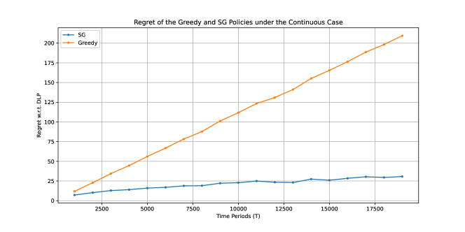
Figure 1: Regret with respect to (DLP) for the Greedy and SG policies.

As one can see from Figure 1, the SG policy achieves a significant lower regret compared to the greedy policy. Moreover, while the regret of the greedy policy grows linearly with time horizon $T$, the regret of the SG policy grows much slower, which echoes with Theorem 1 stating that the upper bound for the regret should grow at a $O(\sqrt{T})$ rate.

5.2 LB Policy in the Discrete Case

Then we study the performance of the LB policy (Algorithm 3) when the incoming $\alpha$-cost follows a discrete distribution. For the LB policy, we compare it with five policies, namely the Frequent Resolving (FR), Infrequent Resolving (IFR), Frequent Resolving with Threshold (FRT), Bayesian Selector (Bayes), and Static Greedy (SG). FR, IFR, FRT, and Bayes are four existing resolving heuristics introduced in Section 4.1, which have been proven to achieve a constant regret in canonical online resource allocation problems. SG is Algorithm 1 applied to the discrete case.

We conduct the experiment in two settings. In the first setting, we set the $\alpha$-cost taking values in $[-2,3,4]$ with probability $[0.6,0.3,0.1]$. One can easily scale the $\alpha$-cost to let it take values in $[-1,1]$ and we omit that for demonstration purpose. Here, the accumulated $\alpha$-cost equals to $\Delta_{1}=-1.2,\Delta_{2}=-0.3,\Delta_{3}=0.1$, which are all non-zero, for which we call the example the non-degenerate one. We report the regret of each of the six policy with respect to the (HO_any) upper bound averaged across 100 sample paths in Figure 2.

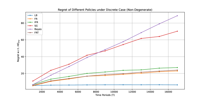
Figure 2: Regret with respect to the (HO_any) for different policies. Here, the $\alpha$-cost takes values in $[-2,3,4]$ with probability $[0.6,0.3,0.1]$.

In the second experiment, we let the $\alpha$-cost $a^{(t)}$ take values in $[-2,1,3,6,8]$ with probability $[0.5,0.1,0.1,0.1,0.2]$. Now the cumulative $\alpha$-cost becomes $\Delta_{1}=-1,\Delta_{2}=-0.9,\Delta_{3}=-0.6,\Delta_{4}=0,\Delta_{5}=1.6$. Note that now because $\Delta_{4}=0$, we call the case degenerate. The problem in this case is inherently harder than the previous one as it is easier for the policy to over-accept the low-cost arrivals, leaving little budgets for future high-cost arrivals. We demonstrate the regret of each of the five policy with respect to the (HO_any) upper bound averaged across 100 sample paths in Figure 3. Here, the regret of Bayes and FRT coincides as they both tend to reject high-cost arrivals more often.

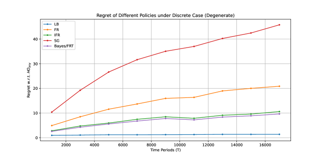
Figure 3: Regret with respect to the (HO_any) for different policies in the degenerate case. Here, the $\alpha$-cost takes values in $[-2,1,3,6,8]$ with probability $[0.5,0.1,0.1,0.1,0.2]$.

From Figure 2 and Figure 3, we make the following observations. (1) The regret of the LB policy remains the lowest and does not grow much with the time horizon. This validats Theorem 3 where we prove the regret grows at a rate of $O(\ln^{2}T)$. (2) The regret of all other policies grow at a faster rate, mostly at a $\Omega(\sqrt{T})$ rate, but some even grows linearly with respect to the time horizon (Bayes in the first setting). (3) The performance of some policies can be fragile to the cost distribution. For example, while Bayes performs well in the second setting, it has linear regret in the first one. Also, even though FR performs better in the non-degenerate case, it can have poor performance in the degenerate setting.

5.3 Lower Bound Validation

Finally, we conduct a small experiment to validate the lower bound we provide in Theorem 2. In particular, for each distribution $\mathcal{D}_{T}$ indexed by $T$, we let it take values in $[-1,1,3]$ with probability $[1/2+1/\sqrt{T},1/2-2/\sqrt{T},1/\sqrt{T}]$. Then we calculate the gap between the optimal dynamic programming solution (DP) and the (HO_any) upper bound. Essentially, (DP) is the best online policy one can get without referring to the future information, and so the gap demonstrate the inherent difficulty of the online problem with respect to the offline counterpart. We take the average of 1000 sample paths and plot the log-log plot of the gap relative to the time horizon in Figure 4.

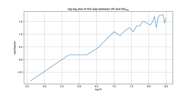
Figure 4: Gap between (HO_any) and (DP). Here, the $T$th distribution is $\mathcal{D}_{T}$, which takes values in $[-1,1,3]$ with probability $[1/2+1/\sqrt{T},1/2-2/\sqrt{T},1/\sqrt{T}]$.

From Figure 4, we can directly see that the $\log(\mbox{Regret})$ and the $\log t$ grows in a linear fashion with the slope being roughly $1/2$. This validates our proof in Theorem 2 that there exists a sequence of distribution such that the gap between the (DP) solution and the (HO_any) solution is $\Omega(\sqrt{T})$.

6 Conclusion

In this paper, we study the problem of optimal policy design for online multiple testing. The goal for the experimenter is to maximize the number of discoveries while ensuring the local false discovery rate is below a pre-specified threshold. We approach this problem through the lens of online resource allocation and formulate the problem as a knapsack problem with negative costs. Our investigation covers two main scenarios where the distribution of the incoming cost is either general or discrete.

For the general distribution, we propose the Static Greedy (SG) policy, showing it achieves a $O(\sqrt{T})$ regret with respect to the offline upper bound. For the discrete distribution, we propose the Logarithm Buffer (LB) policy that achieves a near-optimal regret of order $O(\ln^{2}T)$. Interestingly, existing state-of-the-art policies that achieve constant regrets in the network revenue management problem fail in our setting as they are shown to achieve $\Omega(\sqrt{T})$ or even $\Omega(T)$ regret. The cause if that these policies are too optimistic about future replenishment and can over accept arrivals.

Ongoing work involves extending our new techniques and results to the setting where each arrival at time $t$ is entitled with a reward $r^{(t)}$. Also, it is intriguing to see if we can obtain better instance-dependent regret bounds in the discrete case. We hope this work shed some light on both the online multiple testing problem and the online resource allocation problem with random replenishment. From the online testing perspective, this work may demonstrate the value of applying operations research tools for optimal policy design to improve the power of testing procedures. For the online resource allocation community, this work may provide some insights along with technical novelty to handling the problem where there is a random replenishment of resources. Through these dual lenses, we hope our study contribute to a deeper understanding of both domains, offering some insights that bridge theoretical rigor with practical applications.

Appendix A Proof of Main Results

A.1 Proof of Theorem 1

For simplicity of notation, we write $x^{*}=x^{*}(\bar{a})$ and $p^{*}=\mathbb{P}(A=\bar{a})$. By the design of SG, each time when $a^{(t)}=\bar{a}$, we sample an independent uniform random variable $u^{(t)}$ and accept $a^{(t)}$ if and only if $u^{(t)}\leq x^{*}$. Thus,

$$f_{\mathcal{D}}^{T}(\textbf{SG}) =\mathbb{E}\left[\sum_{t=1}^{T}\mathbbm{1}\{B^{(t)}\geq a^{(t)}\}\left(\mathbbm{1}\{a^{(t)}<\bar{a}\}+\mathbbm{1}\{a^{(t)}=\bar{a},u^{(t)}\leq x^{*}\}\right)\right]$$ (16)

Meanwhile, by the nature of SG, we know that

$$f_{\mathcal{D}}^{T}(\textbf{SG})=T\cdot\left(\mathbb{P}\left(A<\bar{a}\right)+p^{*}x^{*}\right)=\mathbb{E}\left[\sum_{t=1}^{T}\left(\mathbbm{1}\{a^{(t)}<\bar{a}\}+\mathbbm{1}\{a^{(t)}=\bar{a},u^{(t)}\leq x^{*}\}\right)\right].$$ (17)

Combining (16) and (17) we have

$$f_{\mathcal{D}}^{T}(\text{{DLP}})-f_{\mathcal{D}}^{T}(\textbf{SG}) =\mathbb{E}\left[\sum_{t=1}^{T}\mathbbm{1}\{B^{(t)}<a^{(t)}\}\left(\mathbbm{1}\{a^{(t)}<\bar{a}\}+\mathbbm{1}\{a^{(t)}=\bar{a},u^{(t)}\leq x^{*}\}\right)\right].$$ (18)

Define a new process $\{\tilde{B}^{(t)}\}_{t}$ as a “coupled” version of the process $\{B^{(t)}\}_{t}$ as follows. $\tilde{B}^{(1)}=B^{(1)}=0$. For general $t\geq 1$, we define

$$\tilde{B}^{(t+1)}=\max\left\{\tilde{B}^{(t)}-a^{(t)}\left(\mathbbm{1}\{a^{(t)}<\bar{a}\}+\mathbbm{1}\{a^{(t)}=\bar{a},u^{(t)}\leq x^{*}\}\right),0\right\}.$$ (19)

That is, for each sample path $\{a^{(t)}\}_{t}$ with $\{u^{(t)}\}_{t}$, in the “coupled” version regardless of the budget, in each time $t$ we always accept the arrival only it satisfies Line 5-8 in Algorithm 1 (here we also couple the random seed when we face $\bar{a}$). If the budget drops below $0$, we restart the budget level as $0$. We now show that for each sample path $\tilde{B}^{(t)}\leq B^{(t)}$ for any $t$ via induction. Apparently $\tilde{B}^{(1)}\leq B^{(1)}$. Suppose we have $\tilde{B}^{(t)}\leq B^{(t)}$. If at time $t$ the arrival $a^{(t)}$ is rejected by SG, then it implies $a^{(t)}>0$. We have $\tilde{B}^{(t+1)}\leq\tilde{B}^{(t)}\leq B^{(t)}=B^{(t+1)}$. If the arrival is accepted by SG, then we also have

$$\tilde{B}^{(t+1)} =\max\left\{\tilde{B}^{(t)}-a^{(t)}\left(\mathbbm{1}\{a^{(t)}<\bar{a}\}+\mathbbm{1}\{a^{(t)}=\bar{a},u^{(t)}\leq x^{*}\}\right),0\right\}$$

$$\leq\max\left\{B^{(t)}-a^{(t)}\left(\mathbbm{1}\{a^{(t)}<\bar{a}\}+\mathbbm{1}\{a^{(t)}=\bar{a},u^{(t)}\leq x^{*}\}\right),0\right\}$$

$$=\max\left\{B^{(t+1)},0\right\}$$

$$=B^{(t+1)}.$$

This leads to

$$\mathbbm{1}\left\{B^{(t)}<a^{(t)}\right\}\leq\mathbbm{1}\left\{\tilde{B}^{(t)}<a^{(t)}\right\}.$$ (20)

Define $X^{(t)}=-a^{(t)}\left(\mathbbm{1}\{a^{(t)}<\bar{a}\}+\mathbbm{1}\{a^{(t)}=\bar{a},u^{(t)}\leq x^{*}\}\right)$, then we know that $\{X^{(t)}-\mathbb{E}\left[X^{(t)}\right]\}_{t=1,\cdots}$ are i.i.d. random variables bounded within $[-1,1]$. By Proposition 6.2 in Asmussen et al., (2003), we have

$$\tilde{B}^{(t)}=\max\{0,X_{t-1},X_{t-1}+X_{t-2},\cdots,X_{t-1}+\cdots+X_{1}\}$$

is the maximum of the first $t$ positions of a random walk with a non-negative trend. By Lemma 6, we know that for any $a>0$,

$$\mathbb{P}(\tilde{B}^{(t)}<a)\leq O\left(\frac{a}{\sigma\sqrt{t}}+\frac{\kappa}{\sqrt{t}}\right).$$

Therefore,

$$\quad\ \mathbb{E}\left[\mathbbm{1}\{B^{(t)}<a^{(t)}\}\left(\mathbbm{1}\{a^{(t)}<\bar{a}\}+\mathbbm{1}\{a^{(t)}=\bar{a},u^{(t)}\leq x^{*}\}\right)\right]$$ (21)

$$\leq\mathbb{E}\left[\mathbbm{1}\{\tilde{B}^{(t)}<a^{(t)}\}\left(\mathbbm{1}\{a^{(t)}<\bar{a}\}+\mathbbm{1}\{a^{(t)}=\bar{a},u^{(t)}\leq x^{*}\}\right)\right]$$

$$=\mathbb{E}\left[\mathbb{E}\left[\mathbbm{1}\{\tilde{B}^{(t)}<a^{(t)}\}\big{|}a^{(t)}\right]\left(\mathbbm{1}\{a^{(t)}<\bar{a}\}+\mathbbm{1}\{a^{(t)}=\bar{a},u^{(t)}\leq x^{*}\}\right)\right]$$

$$=\mathbb{E}\left[O\left(\frac{a^{(t)}}{\sigma\sqrt{t}}+\frac{\kappa}{\sqrt{t}}\right)\left(\mathbbm{1}\{0<a^{(t)}<\bar{a}\}+\mathbbm{1}\{a^{(t)}=\bar{a},u^{(t)}\leq x^{*}\}\right)\right]$$

$$=O\left(\frac{\mathbb{E}\left[a^{(t)}\left(\mathbbm{1}\{0<a^{(t)}<\bar{a}\}+\mathbbm{1}\{a^{(t)}=\bar{a},u^{(t)}\leq x^{*}\}\right)\right]}{\sigma\sqrt{t}}\right)+O\left(\frac{\kappa}{\sqrt{t}}\right)$$

$$=O\left(\frac{\kappa}{\sqrt{t}}\right).$$

Note that $a^{(t)}$ is independent with $\tilde{B}^{(t)}$. In the last inequality, we use the following inequality:

$$\sigma \geq\sqrt{\mathbb{E}\left[|X^{(t)}-\mathbb{E}\left[X^{(t)}\right]|^{2}\left(\mathbbm{1}\{0<a^{(t)}<\bar{a}\}+\mathbbm{1}\{a^{(t)}=\bar{a},u^{(t)}\leq x^{*}\}\right)\right]}$$

$$\geq\sqrt{\mathbb{E}\left[|-a^{(t)}|^{2}\left(\mathbbm{1}\{0<a^{(t)}<\bar{a}\}+\mathbbm{1}\{a^{(t)}=\bar{a},u^{(t)}\leq x^{*}\}\right)\right]}$$

$$\geq\mathbb{E}\left[a^{(t)}\left(\mathbbm{1}\{0<a^{(t)}<\bar{a}\}+\mathbbm{1}\{a^{(t)}=\bar{a},u^{(t)}\leq x^{*}\}\right)\right]$$

Combining (18) and (21) yields

$$f_{\mathcal{D}}^{T}(\text{{DLP}})-f_{\mathcal{D}}^{T}(\textbf{SG})=\sum_{t=1}^{T}\mathbb{E}\left[O\left(\frac{\kappa}{\sqrt{t}}\right)\right]=O(\kappa\sqrt{T}).$$

A.2 Proof of Theorem 2

Consider $\mathcal{D}_{T}$ as the following discrete distribution:

$$a^{(t)}=\left\{\begin{matrix}&-1/5\triangleq a_{0}&\text{w.p. }1/2+1/\sqrt{T},\\ &1/5\triangleq a_{1}&\text{w.p. }1/2-2/\sqrt{T},\\ &3/5\triangleq a_{2}&\text{w.p. }1/\sqrt{T}.\end{matrix}\right.$$ (22)

Solving DLP yields $x^{*}(-1/5)=x^{*}(1/5)=x^{*}(3/5)=1$.

First, we point out that in the optimal online policy, every arrival of type $a_{1}$ will be accepted as long as the budget is positive. To prove this, it suffices to show that the probability of wrong accept is $0$. In fact, by Lemma 2, the probability of wrongly accept $a^{(t)}$ when $a^{(t)}=1$ can be written as

$$\textit{PWA}_{1}^{(t)} \leq\mathbb{P}\left({B^{(t)}-1<\max_{s\in[t+1,T]}\sum_{r=t+1}^{s}a^{(r)}\mathbbm{1}\{a^{(r)}<1\}}\right)$$

$$\leq\mathbb{P}\left({0<\max_{s\in[t+1,T]}\sum_{r=t+1}^{s}a^{(r)}\mathbbm{1}\{a^{(r)}<1\}}\right)$$

$$=0.$$

From now on we only consider policies that always accept $a^{(t)}$ if $a^{(t)}=a_{1}$. We now provide a property of $B^{(t)}$.

Claim 0.

There exists absolute constants $c_{1}$, $c_{2}$, $c_{3}$, $c_{4}$ such that for any fixed $t\in[T/4,T/2)$:

$$\mathbb{P}\left({a_{2}+c_{1}\sqrt{t}\leq B^{(t)}\leq c_{2}\sqrt{t}}\right)\geq c_{3}-c_{4}/\sqrt{t}.$$

Construct $\underline{B}^{(t)}$ as a “coupled” version of $B^{(t)}$: $\underline{B}^{(1)}=B^{(1)}=0,\underline{B}^{(t+1)}=\max\{\underline{B}^{(t)}-a^{(t)},0\}$. Following the similar argument in the proof of Theorem 1, we know that $\underline{B}^{(t)}$ is a sample path-wise lower bound of $B^{(t)}$, and that

$$\underline{B}^{(t)}=\max\{0,-a^{(t-1)},-a^{(t-1)}-a^{(t-2)},\cdots,-a^{(t-1)}-\cdots-a^{(1)}\}.$$

Let $c_{1}>0$ be some small positive constant to be determined, From Lemma 6, we know that

$$\mathbb{P}\left({B^{(t)}\leq a_{2}+c_{1}\sqrt{t}}\right)\leq\mathbb{P}\left({\underline{B}^{(t)}\leq a_{2}+c_{1}\sqrt{t}}\right)=O\left({\frac{a_{2}+c_{1}\sqrt{t}}{\sqrt{t-1}}+\frac{1}{\sqrt{t}}}\right)=O(c_{1})+O(1/\sqrt{t}),$$ (23)

where in $O(\cdot)$ we hiding absolute constants.

Construct $\overline{B}^{(t)}$ as a “coupled” version of $B^{(t)}$: $\overline{B}^{(1)}=B^{(1)}=0,\overline{B}^{(t+1)}=\max\{\overline{B}^{(t)}-a^{(t)}\mathbbm{1}\{a^{(t)}\leq a_{1}\},3\}$. Following the similar argument in the proof of Theorem 1, we know $\overline{B}^{(t)}$ is a sample path-wise upper bound of $B^{(t)}$, and

$$\overline{B}^{(t)} =\max\left\{3,3-a^{(t-1)}\mathbbm{1}\{a^{(t-1)}\leq a_{1}\},\cdots,3-a^{(t-1)}\mathbbm{1}\{a^{(t-1)}\leq a_{1}\}-\cdots-a^{(1)}\mathbbm{1}\{a^{(1)}\leq a_{1}\}\right\}$$

$$\leq\max\left\{3,3-a^{(t-1)}+\frac{a_{2}}{\sqrt{T}},\cdots,3-a^{(t-1)}-\cdots-a^{(1)}+\frac{(t-1)a_{2}}{\sqrt{T}}\right\}$$

$$\leq 3+\frac{t}{\sqrt{T}}+\max\left\{0,-a^{(t-1)},\cdots,-a^{(t-1)}-\cdots-a^{(1)}\right\}$$

$$\leq 4\sqrt{t}+\max\left\{0,-a^{(t-1)},\cdots,-a^{(t-1)}-\cdots-a^{(1)}\right\}$$

Let $c_{2}>4$ be some large positive constant to be determined. From Lemma 6, we know that

$$\quad\ \mathbb{P}\left({B^{(t)}\geq c_{2}\sqrt{t}}\right)$$ (24)

$$\leq\mathbb{P}\left({\overline{B}^{(t)}\geq c_{2}\sqrt{t}}\right)$$

$$\leq\mathbb{P}\left({\overline{B}^{(t)}-4\sqrt{t}\geq(c_{2}-4)\sqrt{t}}\right)$$

$$=O\left({\bar{\Phi}^{c}\left({\frac{(c_{2}-4)\sqrt{t}}{\sqrt{t-1}}}\right)+\frac{1}{\sqrt{t}}}\right)$$

$$=O(\bar{\Phi}^{c}(c_{2}-4))+O(1/\sqrt{t}),$$

where in $O(\cdot)$ we hiding absolute constants.

Therefore, combining (23) and (24) yields

$$\mathbb{P}\left({a_{2}+c_{1}\sqrt{t}\leq B^{(t)}\leq c_{2}\sqrt{t}}\right)=1-O\left({c_{1}+\bar{\Phi}^{c}(c_{2}-4)}\right)-O\left({1/\sqrt{t}}\right),$$

where in $O(\cdot)$ we are hiding absolute constants. It suffices to take $c_{1}$ to be small enough and $c_{2}$ to be large enough.

We then consider the loss incurred by wrongly accepting or rejecting arrivals of type $a_{2}$.

Claim 1.

For $1\leq t<T/2$, we have

$$\textit{PWA}_{2}^{(t)} \geq\mathbb{P}\left({\left.2B^{(t)}<\sum_{r=t+1}^{t+\lfloor T/2\rfloor}a^{(r)}\mathbbm{1}\{a^{(r)}<a_{2}\},\pi\text{ accepts }a^{(t)}\right|a^{(t)}=a_{2}}\right)$$

In fact, let’s assume the event in Claim 1 happens. This means that standing at time $t$ with budget $B^{(t)}$, from time $t+1$ to $t+\lfloor T/2\rfloor$, only accepting $-1/5$ and $1/5$ will reduce the budget to $-B^{(t)}$ (which is not feasible for an online policy). Now consider $\text{{MIX}}^{(t)}$ (remember in $\text{{MIX}}^{(t)}$ we follow $\pi$ until time $t$, and so in $\text{{MIX}}^{(t)}$ $a^{(t)}$ is accepted). The statement above indicates that in $\text{{MIX}}^{(t)}$ we accept a small number of arrivals of type $a_{1}$ during time $[t+1,t+\lfloor T/2\rfloor]$. In fact, at least $2$ of the arrivals of type $a_{1}$ during time $[t+1,t+\lfloor T/2\rfloor]$ must be rejected. Otherwise, the remaining budget at time $t+\lfloor T/2\rfloor+1$ is at most

$$B^{(t)}-\left({\sum_{r=t+1}^{t+\lfloor T/2\rfloor}a^{(r)}\mathbbm{1}\{a^{(r)}<a_{2}\}-1/5}\right)<1/5-B^{(t)}<0,$$

where in the last inequality we have used the fact that $B^{(t)}>1/5$ because $a^{(t)}$ is accepted. Now consider the following “modification” of $\text{{MIX}}^{(t)}$: instead of accepting $a^{(t)}=a_{2}$ at time $t$, we accept two more arrivals of type $a_{1}$ during time $[t+1,t+\lfloor T/2\rfloor]$. This will not violate the any-time constraint, since $a_{2}>2a_{1}$ and we postpone depleting the budget to later time periods. Apparently, this indicates that the total number of accepted requests induced by $\text{{MIX}}^{(t-1)}$ must be strictly larger than that of $\text{{MIX}}^{(t)}$ — accepting $a^{(t)}$ is a wrong decision.

Claim 2.

For $1\leq t<T/2$, we have

$$\textit{PWR}_{2}^{(t)}\geq\mathbb{P}\left({\left.B^{(t)}-a_{2}\leq\max_{s\in[t+1,T]}\sum_{r=t+1}^{s}a^{(r)},\pi\text{ rejects }a^{(t)}\right|a^{(t)}=a_{2}}\right)$$

In fact, let’s assume the event in Claim 2 happens. It indicates that always accepting the arrivals can never violate the any-time constraint. Therefore, rejecting $a^{(t)}$ is a wrong decision.

Now let’s bound the terms in Claim 1 and 2 separately. Fix $t\in[T/4,T/2)$.

$$\textit{PWA}_{2}^{(t)} \geq\mathbb{P}\left({\left.2B^{(t)}<\sum_{r=t+1}^{t+\lfloor T/2\rfloor}a^{(r)}\mathbbm{1}\{a^{(r)}<a_{2}\},\pi\text{ accepts }a^{(t)}\right|a^{(t)}=a_{2}}\right)$$ (25)

$$\geq\mathbb{P}\left({\left.2B^{(t)}<\sum_{r=t+1}^{t+\lfloor T/2\rfloor}a^{(r)}\mathbbm{1}\{a^{(r)}<a_{2}\},B^{(t)}\leq c_{2}\sqrt{t},\pi\text{ accepts }a^{(t)}\right|a^{(t)}=a_{2}}\right)$$

$$\geq\mathbb{P}\left({\left.2c_{2}\sqrt{t}<\sum_{r=t+1}^{t+\lfloor T/2\rfloor}a^{(r)}\mathbbm{1}\{a^{(r)}<a_{2}\},B^{(t)}\leq c_{2}\sqrt{t},\pi\text{ accepts }a^{(t)}\right|a^{(t)}=a_{2}}\right)$$

$$=\mathbb{P}\left({2c_{2}\sqrt{t}<\sum_{r=t+1}^{t+\lfloor T/2\rfloor}a^{(r)}\mathbbm{1}\{a^{(r)}<a_{2}\}}\right)\mathbb{P}\left({\left.B^{(t)}\leq c_{2}\sqrt{t},\pi\text{ accepts }a^{(t)}\right|a^{(t)}=a_{2}}\right)$$

$$\geq\mathbb{P}\left({\sum_{r=t+1}^{t+\lfloor T/2\rfloor}\left({a^{(r)}\mathbbm{1}\{a^{(r)}<a_{2}\}+a_{2}/\sqrt{T}}\right)>3c_{2}\sqrt{T}}\right)\mathbb{P}\left({\left.B^{(t)}\leq c_{2}\sqrt{t},\pi\text{ accepts }a^{(t)}\right|a^{(t)}=a_{2}}\right)$$

$$=\left({\Omega(1)-O(1/\sqrt{T})}\right)\mathbb{P}\left({\left.B^{(t)}\leq c_{2}\sqrt{t},\pi\text{ accepts }a^{(t)}\right|a^{(t)}=a_{2}}\right).$$

Note that in the last equality we have applied the Berry-Esseen theorem to give a lower bound for deviation of sum of i.i.d. random variables. In $\Omega(\cdot)$ and $O(\cdot)$ we are hiding absolute constants.

$$\textit{PWR}_{2}^{(t)} \geq\mathbb{P}\left({\left.B^{(t)}-a_{2}\geq\max_{s\in[t+1,T]}\sum_{r=t+1}^{s}a^{(r)},\pi\text{ rejects }a^{(t)}\right|a^{(t)}=a_{2}}\right)$$ (26)

$$\geq\mathbb{P}\left({\left.B^{(t)}-a_{2}\geq\max_{s\in[t+1,T]}\sum_{r=t+1}^{s}a^{(r)},B^{(t)}\geq a_{2}+c_{1}\sqrt{t},\pi\text{ rejects }a^{(t)}\right|a^{(t)}=a_{2}}\right)$$

$$\geq\mathbb{P}\left({\left.c_{1}\sqrt{t}\geq\max_{s\in[t+1,T]}\sum_{r=t+1}^{s}a^{(r)},B^{(t)}\geq a_{2}+c_{1}\sqrt{t},\pi\text{ rejects }a^{(t)}\right|a^{(t)}=a_{2}}\right)$$

$$=\mathbb{P}\left({c_{1}\sqrt{t}\geq\max_{s\in[t+1,T]}\sum_{r=t+1}^{s}a^{(r)}}\right)\mathbb{P}\left({\left.B^{(t)}\geq c_{1}\sqrt{t},\pi\text{ rejects }a^{(t)}\right|a^{(t)}=a_{2}}\right)$$

$$\geq\mathbb{P}\left({c_{1}\sqrt{T-t}/2\geq\max_{s\in[t+1,T]}\sum_{r=t+1}^{s}a^{(r)}}\right)\mathbb{P}\left({\left.B^{(t)}\geq c_{1}\sqrt{t},\pi\text{ rejects }a^{(t)}\right|a^{(t)}=a_{2}}\right)$$

$$=\left({\Omega(1)-O(1/\sqrt{T-t})}\right)\mathbb{P}\left({\left.B^{(t)}\geq c_{1}\sqrt{t},\pi\text{ rejects }a^{(t)}\right|a^{(t)}=a_{2}}\right).$$

Note that in the last equality we have applied Lemma 6. In $\Omega(\cdot)$ and $O(\cdot)$ we are hiding absolute constants.

Combining (25) and (26) we have for $t\in[T/4,T/2)$:

$$\quad\ \textit{PWA}_{2}^{(t)}+\textit{PWR}_{2}^{(t)}$$

$$\geq\left({\Omega(1)-O(1/\sqrt{T})}\right)\mathbb{P}\left({\left.B^{(t)}\leq c_{2}\sqrt{t},\pi\text{ accepts }a^{(t)}\right|a^{(t)}=a_{2}}\right)+$$

$$\quad\ \quad\ \left({\Omega(1)-O(1/\sqrt{T-t})}\right)\mathbb{P}\left({\left.B^{(t)}\geq a_{2}+c_{1}\sqrt{t},\pi\text{ rejects }a^{(t)}\right|a^{(t)}=a_{2}}\right)$$

$$=\left({\Omega(1)-O(1/\sqrt{T})}\right)\left(\mathbb{P}\left({\left.B^{(t)}\leq c_{2}\sqrt{t},\pi\text{ accepts }a^{(t)}\right|a^{(t)}=a_{2}}\right)+\right.$$

$$\quad\ \quad\ \quad\ \left.\mathbb{P}\left({\left.B^{(t)}\geq a_{2}+c_{1}\sqrt{t},\pi\text{ rejects }a^{(t)}\right|a^{(t)}=a_{2}}\right)\right)$$

$$=\left({\Omega(1)-O(1/\sqrt{T})}\right)\left(\mathbb{P}\left({\left.\pi\text{ accepts }a^{(t)}\right|a^{(t)}=a_{2}}\right)-\mathbb{P}\left({\left.B^{(t)}>c_{2}\sqrt{t},\pi\text{ accepts }a^{(t)}\right|a^{(t)}=a_{2}}\right)+\right.$$

$$\quad\ \quad\ \quad\ \left.\mathbb{P}\left({\left.\pi\text{ rejects }a^{(t)}\right|a^{(t)}=a_{2}}\right)-\mathbb{P}\left({\left.B^{(t)}<a_{2}+c_{1}\sqrt{t},\pi\text{ rejects }a^{(t)}\right|a^{(t)}=a_{2}}\right)\right)$$

$$\geq\left({\Omega(1)-O(1/\sqrt{T})}\right)\left(1-\mathbb{P}\left({\left.B^{(t)}>c_{2}\sqrt{t}\right|a^{(t)}=a_{2}}\right)-\mathbb{P}\left({\left.B^{(t)}<a_{2}+c_{1}\sqrt{t}\right|a^{(t)}=a_{2}}\right)\right)$$

$$=\left({\Omega(1)-O(1/\sqrt{T})}\right)\mathbb{P}\left({\left.a_{2}+c_{1}\sqrt{t}\leq B^{(t)}\leq c_{2}\sqrt{t}\right|a^{(t)}=a_{2}}\right)$$

$$=\left({\Omega(1)-O(1/\sqrt{T})}\right)\mathbb{P}\left({a_{2}+c_{1}\sqrt{t}\leq B^{(t)}\leq c_{2}\sqrt{t}}\right)$$

$$=\left({\Omega(1)-O(1/\sqrt{T})}\right)\left({\Omega(1)-O(1/\sqrt{t})}\right)$$

$$=\Omega(1)-O(1/\sqrt{T}).$$

In $\Omega(\cdot)$ and $O(\cdot)$ we are hiding absolute constants.

Now it’s time to wrap up. The total expected loss incurred by wrongly accepting or rejecting arrivals of type $a_{2}$ is at least

$$\quad\ \sum_{\frac{T}{4}\leq t<T/2}p_{2}\left({\textit{PWA}_{2}^{(t)}+\textit{PWR}_{2}^{(t)}}\right)$$

$$=\Omega(T)\cdot\frac{1}{\sqrt{T}}\cdot\left({\Omega(1)-O(1/\sqrt{T})}\right)$$

$$=\Omega(\sqrt{T}).$$

In $\Omega(\cdot)$ and $O(\cdot)$ we are hiding absolute constants.

A.3 Proof of Proposition 2

Consider the example $(a_{-1},a_{1})=(-1,1)$ and $(p_{-1},p_{1})=(-1,1)$, which is a simple random walk. In this case, by solving DLP, the DLP directly leads to $x_{\text{{DLP}}}^{(T)}=(T/2,T/2)$ nad $f(\text{{DLP}})=T$. Solving the offline problem (HO_any) leads to:

$$x_{\textbf{HO\textsubscript{fix}}}^{(T)}(-1|\mathcal{W}^{(T)}) =\Lambda^{[1,T]}(-1|\mathcal{W}^{(T)}),$$

$$x_{\textbf{HO\textsubscript{fix}}}^{(T)}(1|\mathcal{W}^{(T)}) =\min\{\Lambda^{[1,T]}(-1|\mathcal{W}^{(T)}),$$

$$\Lambda^{[1,T]}(1|\mathcal{W}^{(T)})\} =T-\max\{\Lambda^{[1,T]}(1|\mathcal{W}^{(T)})-\Lambda^{[1,T]}(-1|\mathcal{W}^{(T)}),0\}.$$

Note that the quantity $\left|\Lambda^{[1,T]}(-1|\mathcal{W}^{(T)})-\Lambda^{[1,T]}(1|\mathcal{W}^{(T)})\right|$ is the distance from zero at time $T$ of a simple random walk, which is well-known as $\Omega(\sqrt{T})$ (Durrett,, 2019).

Furthermore, in the context of a simple random walk, the first constraint in (HO_any) can be interpreted as follows: a walker starts at point 0 and, from time 1 to $T$, receives steps from the set $\{-1,+1\}$, deciding whether to accept each step. The walker cannot move right of 0, with the objective being to maximize the number of accepted steps. A greedy policy — where the walker rejects a step if and only if it is currently at zero and the step is $+1$ — simplifies the process to a simple random walk with a wall at zero. This is sometimes called The next lemma simplifies the difference $f(\textbf{HO\textsubscript{fix}}|\mathcal{W}^{(T)})-f(\textbf{HO\textsubscript{any}}|\mathcal{W}^{(T)})$ to a property of the reflected simple random walks. We then show that $f(\textbf{HO\textsubscript{fix}}|\mathcal{W}^{(T)})-f(\textbf{HO\textsubscript{any}}|\mathcal{W}^{(T)})$ has the same distribution with the distance of the walker from zero at time $T$.

Lemma 3.

Denote $D_{r}(T)$ as the distance of the walker from zero at time $T$ and $S_{r}(T)$ as the total length of time of the walker stopping at zero by time $T$, respectively in the random walk described above. Then we have

• $S_{r}(T)-D_{r}(T)=\Lambda^{[1,T]}(1|\mathcal{W}^{(T)})-\Lambda^{[1,T]}(-1|\mathcal{W}^{(T)})$;

• $f(\textbf{HO\textsubscript{fix}}|\mathcal{W}^{(T)})-f(\textbf{HO\textsubscript{any}}|\mathcal{W}^{(T)})=\min\{D_{r}(T),S_{r}(T)\}.$

By Lemma 3, it follows that

$$f(\textbf{HO\textsubscript{fix}}|\mathcal{W}^{(T)})-f(\textbf{HO\textsubscript{any}}|\mathcal{W}^{(T)})=D_{r}(T)-\max\{\Lambda^{[1,T]}(-1|\mathcal{W}^{(T)})-\Lambda^{[1,T]}(1|\mathcal{W}^{(T)}),0\}.$$

Thereforoe, it is enough to show that $\mathbb{E}\left[D_{r}(T)-\max\{\Lambda^{[1,T]}(-1|\mathcal{W}^{(T)})-\Lambda^{[1,T]}(1|\mathcal{W}^{(T)}),0\}\right]=\Omega(\sqrt{T})$.

Note that $D_{r}(t+1)=\max\{D_{r}(t)-a^{(t+1)},0\}=\max\{D_{r}(t)+\Lambda^{[t+1,t+1]}(-1|\mathcal{W}^{(T)})-\Lambda^{[t+1,t+1]}(1|\mathcal{W}^{(T)}),0\}$ by definition. If follows that $\{D_{r}(t)\}_{t=0}^{\infty}$ is a Lindley process. By Proposition 6.3 in Asmussen et al., (2003), we have

$$D_{r}(t+1)=\max\{ \Lambda^{[t+1,t+1]}(-1|\mathcal{W}^{(T)})-\Lambda^{[t+1,t+1]}(1|\mathcal{W}^{(T)}),\Lambda^{[t,t+1]}(-1|\mathcal{W}^{(T)})-\Lambda^{[t,t+1]}(1|\mathcal{W}^{(T)}),\dots,$$

$$\Lambda^{[1,t+1]}(-1|\mathcal{W}^{(T)})-\Lambda^{[1,t+1]}(1|\mathcal{W}^{(T)}),0\}.$$

Therefore, we only need to prove that

$$\mathbb{E}\left[\max_{t\in[T]}\{\Lambda^{[t,T]}(-1|\mathcal{W}^{(T)})-\Lambda^{[t,T]}(1|\mathcal{W}^{(T)}),0\}\right]-\mathbb{E}\left[\max\{\Lambda^{[1,T]}(-1|\mathcal{W}^{(T)})-\Lambda^{[1,T]}(1|\mathcal{W}^{(T)}),0\}\right]=\Omega(\sqrt{T}).$$

By the reflection principle of simple random walk (Durrett,, 2019), we have

$$\quad\ \mathbb{P}\left({\max_{t\in[T]}\{\Lambda^{[t,T]}(-1|\mathcal{W}^{(T)})-\Lambda^{[t,T]}(1|\mathcal{W}^{(T)}),0\}\geq a}\right)$$

$$=2\mathbb{P}\left({\max\{\Lambda^{[1,T]}(-1|\mathcal{W}^{(T)})-\Lambda^{[1,T]}(1|\mathcal{W}^{(T)}),0\}\geq a}\right),\quad\forall a>0.$$

Hence, it follows that

$$\mathbb{E}\left[\max_{t\in[T]}\{\Lambda^{[t,T]}(-1|\mathcal{W}^{(T)})-\Lambda^{[t,T]}(1|\mathcal{W}^{(T)}),0\}\right] \overset{(*)}{=}\sum_{a=1}^{\infty}\mathbb{P}\left({\max_{t\in[T]}\{\Lambda^{[t,T]}(-1|\mathcal{W}^{(T)})-\Lambda^{[t,T]}(1|\mathcal{W}^{(T)}),0\}\geq aa}\right)$$

$$=\sum_{a=1}^{\infty}2\mathbb{P}\left({\max\{\Lambda^{[1,T]}(-1|\mathcal{W}^{(T)})-\Lambda^{[1,T]}(1|\mathcal{W}^{(T)}),0\}\geq a}\right)$$

$$=2\mathbb{E}\left[\max_{t\in[T]}\{\Lambda^{[t,T]}(-1|\mathcal{W}^{(T)})-\Lambda^{[t,T]}(1|\mathcal{W}^{(T)}),0\}\right],$$

where $(*)$ uses the equation

$$\mathbb{E}\left[A\right]=\sum_{a=0}^{\infty}a\mathbb{P}(A=a)=\sum_{a^{\prime}=1}^{\infty}\mathbb{P}(A\geq a^{\prime}).$$

As a result, we get

$$\mathbb{E}\left[\max_{t\in[T]}\{\Lambda^{[t,T]}(-1|\mathcal{W}^{(T)})-\Lambda^{[t,T]}(1|\mathcal{W}^{(T)}),0\}\right]-\mathbb{E}\left[\max\{\Lambda^{[1,T]}(-1|\mathcal{W}^{(T)})-\Lambda^{[1,T]}(1|\mathcal{W}^{(T)}),0\}\right]$$

$$=\mathbb{E}\left[\max\{\Lambda^{[1,T]}(-1|\mathcal{W}^{(T)})-\Lambda^{[1,T]}(1|\mathcal{W}^{(T)}),0\}\right]$$

$$=\Omega(\sqrt{T}),$$

where the last equation is derived by the Central Limit Theorem (Durrett,, 2019).

A.4 Proof of Proposition 3

Instance (i): $a=[-1/2,1/2,1],p=[0.6,0.2,0.2]$.

Solving DLP yields $x^{*}=[1,1,1]$. Then the four policies all degenerate to the greedy policy, i.e. accept all arrivals whenever the budget is available. Following the proof of Theorem 3, we define $\text{{MIX}}^{(t)}$ as the policy that applying greedy policy in time $[1,t]$ and applying offline optimal policy $\textbf{HO\textsubscript{any}}^{([t+1,T])}$ to the remaining time periods. Specially, define $\text{{MIX}}^{(0)}=\textbf{HO\textsubscript{any}}^{([1,T])}$ as the policy that applying hindsight optimal throughout the process and $\text{{MIX}}^{(T)}=\text{Greedy}^{[1,T]}$ as the policy that applying the greedy policy throughout the process. We restate (14):

$$f(\textbf{HO\textsubscript{any}})-f(\textbf{FR})=\mathbb{E}\left[\sum_{t=1}^{T}\left[{f(\text{{MIX}}^{(t-1)}\big{|}\mathcal{W}^{(T)})-f(\text{{MIX}}^{(t)}\big{|}\mathcal{W}^{(T)})}\right]\right].$$ (27)

It directly follows from the definition of $f$ that

$$f(\text{{MIX}}^{(t-1)}\big{|}\mathcal{W}^{(T)})-f(\text{{MIX}}^{(t)}\big{|}\mathcal{W}^{(T)})$$

$$=\mathbbm{1}\{\text{{MIX}}^{(t)}\text{ wrongly accepts }a^{(t)}\}+\mathbbm{1}\{\text{{MIX}}^{(t)}\text{ wrongly rejects }a^{(t)}\}.$$

Therefore, we have

$$\quad\ \mathbb{E}\left[f(\text{{MIX}}^{(t-1)}\big{|}\mathcal{W}^{(T)})-f(\text{{MIX}}^{(t)}\big{|}\mathcal{W}^{(T)})\right]$$

$$\geq p_{2}\cdot\mathbb{P}(\text{{MIX}}^{(t)}\text{ wrongly accepts }a^{(t)}|a^{(t)}=a_{2})$$

$$=0.2\cdot\mathbb{P}(\underset{:=\textit{PWR}^{(t)}}{\underbrace{\text{{MIX}}^{(t)}\text{ wrongly accepts }a^{(t)}|a^{(t)}=1}}).$$

In order to give lower bound to the Now we construct a coupling random process $\{\tilde{B}^{(t)}\}_{t=0}^{T}$ such that $\tilde{B}^{(0)}=1$ and $\tilde{B}^{(t+1)}=\max\{B^{(t)}-a^{(t)},1\}$. By induction it is easy to verify that $\tilde{B}^{(t)}\geq B^{(t)},\forall t\geq 0$. By Proposition 6.2 in Asmussen et al., (2003), we have $\tilde{B}^{(t)}\sum\max\{-a^{(t)},-\sum_{s=t-1}^{t}a^{(s)},\dots,-\sum_{s=1}^{t}a^{(s)},1\}$. For $t\geq 2$, applying Lemma 6, there is probability of $\Omega(\frac{1}{\sqrt{t}})$ such that $\tilde{B}^{(t-2)}\leq 1$. Conditioned on this, we have $B^{(t-2)}\leq 1.$ There are three cases: $B^{(t-2)}=0$, $B^{(t-2)}=1/2$ and $B^{(t-2)}=1$. If $B^{(t-2)}=0$, then $B^{(t)}=1$ with probability $0.6*0.6$ of two consecutive arrival $a^{(t-2)}=a^{(t-1)}=-1/2$. Similarly for the other two cases, conditioned on $B^{(t-2)}\leq 1$, there are probability at least $0.2*0.2$ such that $B^{(t)}=1.$ Therefore, we have $\mathbb{P}(B^{(t)}=2)=\Omega(1/\sqrt{t})$. Conditioned on $B^{(t)}=2$, $[a^{(t)},a^{(t+1)},a^{(t+2)}]=[1,1/2,1/2]$ happens with probability $0.2^{3}$. When all the above events happen, it generates a wrong acceptance of $a^{(t)}=1$ because it follows a rejection of two arrivals of cost $1/2$. We then have $\mathbb{P}(\underset{:=\textit{PWR}^{(t)}}{\underbrace{\text{{MIX}}^{(t)}\text{ wrongly accepts }a^{(t)}|a^{(t)}=1}})=\Omega(1/\sqrt{t})$. Combining this result with (27) yields

$$f_{\mathcal{D}}^{T}(\textbf{HO\textsubscript{any}})-f_{\mathcal{D}}^{T}(\textbf{FR})=\Omega(\sum_{t=1}^{T}1/\sqrt{t})=\Omega(\sqrt{T}).$$

Instance (ii): $a=[-1/2,1/2,1],p=[0.5,0.4,0.1]$.

Solving DLP yields $x^{*}=[1,1,1/2]$. Then the Bayes algorithm degenerates to greedy policy, i.e. accept all arrivals when the budget is available. We construct the sequence $\{\tilde{B}^{(t)}\}_{t=0}^{T}$ with the same definition. In this case, since $a\cdot p^{\prime}>0$, applying Lemma 4 leads to $\mathbb{P}(\tilde{B}^{(t-2)}\leq 1)\geq c$ for some constant $c$ independent of $t$. Following a similar argument in instance (i), we have $\mathbb{P}(\underset{:=\textit{PWR}^{(t)}}{\underbrace{\text{{MIX}}^{(t)}\text{ wrongly accepts }a^{(t)}|a^{(t)}=1}})>c^{\prime}$ for some constant $c^{\prime}>0$ independent of $t$. Combining this result with (27) yields

$$f_{\mathcal{D}}^{T}(\textbf{HO\textsubscript{any}})-f_{\mathcal{D}}^{T}(\textbf{FR})=\Omega(T).$$

A.5 Proof of Theorem 3

We begin by giving several lemmas that help us to build up the proof. The first is about the large deviation of i.i.d. random variables (i.e. probability of deviation of order $t$ from partial sum of $t$ i.i.d. random variables).

Lemma 4 (Large deviation I).

Assume $\xi_{1},\dots,\xi_{t},\cdots$ are i.i.d. random variables on $[-1,1]$ with zero mean (i.e. $\mathbb{E}\left[\xi_{1}\right]=0$). Then for any $\epsilon>0,B\geq 0$, we have

$$\mathbb{P}\left({\exists t\geq 1\text{ s.t. }\sum_{s=1}^{t}\xi_{s}\geq B+\epsilon t}\right)\leq\exp\left({-2B\epsilon}\right),\quad\mathbb{P}\left({\exists t\geq 1\text{ s.t. }\sum_{s=1}^{t}\xi_{s}\leq-B-\epsilon t}\right)\leq\exp\left({-2B\epsilon}\right).$$ (28)

Lemma 5 (Large deviation II).

Assume $\xi_{1},\dots,\xi_{t},\cdots$ are i.i.d. random variables on $[-1,1]$ with zero mean (i.e. $\mathbb{E}\left[\xi_{1}\right]=0$). Then for any $t\geq 1$ and $\epsilon>0$, we have

$$\mathbb{P}\left({\exists 1\leq s\leq t\text{ s.t. }\sum_{r=1}^{s}\xi_{s}\geq\epsilon t}\right)\leq\exp\left({-\frac{\epsilon^{2}t}{2}}\right),\quad\mathbb{P}\left({\exists 1\leq s\leq t\text{ s.t. }\sum_{r=1}^{s}\xi_{s}\leq-\epsilon t}\right)\leq\exp\left({-\frac{\epsilon^{2}t}{2}}\right).$$ (29)

Finally, we introduce the following theorem proved in Nagaev, (1970) concerning moderate deviation of i.i.d. random variables, which gives an efficient bound to the maximum of partial sum of zero-mean i.i.d. random variables.

Theorem 4.

Assume $\xi_{1},\dots,\xi_{t}$ are i.i.d. mean zero random variables with $\rho^{3}=\mathbb{E}\left[|\xi_{s}|^{3}\right]<\infty$, $\sigma^{2}=\mathbb{E}\left[\xi_{s}^{2}\right]<\infty$. Then there exists an absolute constant $K$ such that

$$\sup_{0\leq x<\infty}\left|\mathbb{P}\left({\max_{1\leq s\leq t}\sum_{r=1}^{s}\xi_{r}\leq\sigma x\sqrt{t}}\right)-\left({\frac{2}{\pi}}\right)^{1/2}\int_{0}^{x}e^{-u^{2}/2}du\right|<\frac{K\rho^{6}}{\sigma^{6}\sqrt{t}}.$$

For $x\geq 0$, define

$$\bar{\Phi}(x)=\left({\frac{2}{\pi}}\right)^{1/2}\int_{0}^{x}e^{-u^{2}/2}du,\quad\bar{\Phi}^{c}(x)=1-\bar{\Phi}(x)=\left({\frac{2}{\pi}}\right)^{1/2}\int_{x}^{+\infty}e^{-u^{2}/2}du.$$

By setting $x=B/(\sigma\sqrt{t})$ in Theorem 4, we get

$$\frac{K\rho^{6}}{\sigma^{6}\sqrt{t}} >\left|\mathbb{P}\left({\max_{1\leq s\leq t}\sum_{r=1}^{s}\xi_{r}\leq B}\right)-\left({\frac{2}{\pi}}\right)^{1/2}\int_{0}^{B/(\sigma\sqrt{t})}e^{-u^{2}/2}du\right|$$

$$\geq\mathbb{P}\left({\max_{1\leq s\leq t}\sum_{r=1}^{s}\xi_{r}\leq B}\right)-\bar{\Phi}\left({\frac{B}{\sigma\sqrt{t}}}\right)$$

$$\geq\mathbb{P}\left({\max_{1\leq s\leq t}\sum_{r=1}^{s}\xi_{r}\leq B}\right)-\left({\frac{2}{\pi}}\right)^{1/2}B/(\sigma\sqrt{t}).$$

Meanwhile,

$$\frac{K\rho^{6}}{\sigma^{6}\sqrt{t}} >\left|\mathbb{P}\left({\max_{1\leq s\leq t}\sum_{r=1}^{s}\xi_{r}\leq B}\right)-\left({\frac{2}{\pi}}\right)^{1/2}\int_{0}^{B/(\sigma\sqrt{t})}e^{-u^{2}/2}du\right|$$

$$=\left|\left({\frac{2}{\pi}}\right)^{1/2}\int_{B/(\sigma\sqrt{t})}^{+\infty}e^{-u^{2}/2}du-\mathbb{P}\left({\max_{1\leq s\leq t}\sum_{r=1}^{s}\xi_{r}>B}\right)\right|$$

$$\geq\bar{\Phi}^{c}\left({\frac{B}{\sigma\sqrt{t}}}\right)-\mathbb{P}\left({\max_{1\leq s\leq t}\sum_{r=1}^{s}\xi_{r}\leq B}\right).$$

It immediately leads to the following lemma.

Lemma 6.

Assume $\xi_{1},\dots,\xi_{t}$ are i.i.d. random variables on $[-1,1]$ with zero mean (i.e. $\mathbb{E}\left[\xi_{1}\right]=0$). Let $\rho^{3}=\mathbb{E}\left[|\xi_{s}|^{3}\right]<\infty$, $\sigma^{2}=\mathbb{E}\left[\xi_{s}^{2}\right]<\infty$, $\kappa:=\rho^{6}/\sigma^{6}$. Then for any $B>0$, it holds that

$$\mathbb{P}\left({\max_{1\leq s\leq t}\sum_{r=1}^{s}\xi_{r}\leq B}\right) =O\left({\frac{B}{\sigma\sqrt{t}}+\frac{\kappa}{\sqrt{t}}}\right),$$

$$\mathbb{P}\left({\max_{1\leq s\leq t}\sum_{r=1}^{s}\xi_{r}\leq B}\right) =\Omega\left({\bar{\Phi}\left({\frac{B}{\sigma\sqrt{t}}}\right)-\frac{\kappa}{\sqrt{t}}}\right),\quad\mathbb{P}\left({\max_{1\leq s\leq t}\sum_{r=1}^{s}\xi_{r}>B}\right) =\Omega\left({\bar{\Phi}^{c}\left({\frac{B}{\sigma\sqrt{t}}}\right)-\frac{\kappa}{\sqrt{t}}}\right),$$

where in $O(\cdot)$ and $\Omega(\cdot)$ we are hiding absolute constants.

Case I: $i\leq i_{0}$.

In this case, the arrival is of “low cost” type ($\sum_{j=-m}^{i}a_{j}p_{j}<0$).

(i). Let’s first bound $\textit{PWA}_{i}^{(t)}$. We note that when $i=1$, following the proof of Theorem 2, we know that always accepting the lowest cost does no harm. We only consider the case when $i>1$. Note that $a^{(r)}\mathbbm{1}\{a^{(r)}<a_{i}\}$, $r=t+1,\cdots,T$ are i.i.d. random variables with expectation

$$\sum_{j=-m}^{i-1}a_{j}p_{j}\triangleq\Delta_{i-1}<0.$$

Then $a^{(r)}\mathbbm{1}\{a^{(r)}<a_{i}\}-\Delta_{i-1}$ are zero-mean i.i.d. random variables in $[-1,1]$. We can bound $\textit{PWA}_{i}^{(t)}$ by

$$\quad\ \mathbb{P}\left({B^{(t)}-a_{i}<\max_{s\in[t+1,T]}\sum_{r=t+1}^{s}a^{(r)}\mathbbm{1}\{a^{(r)}<a_{i}\},B^{(t)}\geq C_{\textit{low}}\ln(T-t+1)}\right)$$ (30)

$$\leq\mathbb{P}\left({C_{\textit{low}}\ln(T-t+1)-a_{i}<\max_{s\in[t+1,T]}\sum_{r=t+1}^{s}a^{(r)}\mathbbm{1}\{a^{(r)}<a_{i}\}}\right)$$

$$=\mathbb{P}\left({\exists s\in[t+1,T]:\sum_{r=t+1}^{s}\left({a^{(r)}\mathbbm{1}\{a^{(r)}<a_{i}\}-\Delta_{i-1}}\right)>C_{\textit{low}}\ln(T-t+1)-a_{i}-\Delta_{i-1}\cdot(s-t)}\right)$$

$$\leq\exp\left({2(C_{\textit{low}}\ln(T-t+1)-a_{i})\Delta_{i-1}}\right)$$

$$\leq e^{2}(T-t+1)^{2C\Delta_{i-1}}$$

where in the last inequality we use Lemma 4. When $C_{\textit{low}}\geq-\frac{1}{\Delta_{i_{0}-1}}$, we know that

$$e^{2}(T-t+1)^{2C\Delta_{i-1}}\leq e^{2}(T-t+1)^{-2\frac{\Delta_{i-1}}{\Delta_{i_{0}-1}}}=O\left({(T-t+1)^{-2}}\right),$$

where in $O(\cdot)$ we are hiding an absolute constant.

(ii). Let’s first bound $\textit{PWR}_{i}^{(t)}$. It suffices to bound $\mathbb{P}\left({B^{(t)}<C_{\textit{low}}\ln(T-t+1)}\right)$. We cover the event by two parts: (a) $B^{(s)}<C_{\textit{mid}}\ln(T-s+1)$ for $s=1,\dots,t$; (b) there exists $1\leq s\leq t$ such that $B^{(s)}\geq C_{\textit{mid}}\ln(T-s+1)$, and at any time $s^{\prime}\in(s,t]$, the budget is always below $C_{\textit{mid}}\ln(T-s^{\prime})$. Then

$$\quad\ \mathbb{P}(B^{(t)}<C_{\textit{low}}\ln(T-t+1))$$

$$=\mathbb{P}(B^{(t)}<C_{\textit{low}}\ln(T-t+1),\text{ (a) happens})+\mathbb{P}(B^{(t)}<C_{\textit{low}}\ln(T-t+1),\text{ (b) happens}).$$

Consider the situation when event (a) holds. It follows that only type $j\leq i_{0}$ will be accepted throughout time $1$ to $t$. Therefore, we have

$$C_{\textit{low}}\ln(T-t+1)>B^{(t)}=B^{(1)}-\sum_{s=1}^{t}a^{(s)}\mathbbm{1}\{\text{accept $a^{(s)}$}\}\geq-\sum_{s=1}^{t}a^{(s)}\mathbbm{1}\{a^{(s)}\leq a_{i_{0}}\}.$$

Using the fact that $a^{(s)}\mathbbm{1}\{a^{(s)}\leq a_{i_{0}}\}\ (s=1,\cdots,t)$ are i.i.d. random variables in $[-1,1]$ with expectation $\Delta_{i_{0}}$, we get

$$\quad\ \mathbb{P}(B^{(t)}<C_{\textit{low}}\ln(T-t+1),\text{ (a) happens})$$ (31)

$$\leq\mathbb{P}\left({C_{\textit{low}}\ln(T-t+1)\geq-\sum_{s=1}^{t}a^{(s)}\mathbbm{1}\{a^{(s)}\leq a_{i_{0}}\}}\right)$$

$$\leq\mathbb{P}\left({\sum_{s=1}^{t}\left({a^{(s)}\mathbbm{1}\{a^{(s)}\leq a_{i_{0}}\}-\Delta_{i_{0}}}\right)\geq-\Delta_{i_{0}}t-C_{\textit{low}}\ln(T-t+1)}\right)$$

$$\leq\exp\left({-\frac{\left({-\Delta_{i_{0}}t-C_{\textit{low}}\ln T}\right)_{+}^{2}}{2t}}\right).$$

The last inequality holds by the Hoeffding’s inequality.

Consider the situation when event (b) holds, without loss of generality, let $s<t$ be the largest time such that $B^{(s)}\geq C_{\textit{mid}}\ln(T-t+1)$. Then $B^{(r)}<C_{\textit{mid}}\ln(T-r+1)$ and for $s<r\leq t$. It is not difficult to observe that $B^{(s+1)}\geq C_{\textit{mid}}\ln(T-s)-a_{i_{0}+1}\geq C_{\textit{mid}}\ln(T-t+1)-a_{i_{0}+1}$. Thus,

$$(C_{\textit{mid}}-C_{\textit{low}})\ln(T-t+1)-a_{i_{0}+1}\leq B^{(s+1)}-B^{(t)}\leq\sum_{r=s+1}^{t}a^{(r)}\mathbbm{1}\{\text{accept $a^{(r)}$}\}\leq\sum_{r=s+1}^{t}a^{(r)}\mathbbm{1}\{a^{(r)}\leq a_{i_{0}}\}.$$

Therefore,

$$\quad\ \mathbb{P}(B^{(t)}<C_{\textit{low}}\ln(T-t+1),\text{ (b) happens})$$ (32)

$$\leq\mathbb{P}\left({\exists s\in[1,t):\sum_{r=s+1}^{t}a^{(r)}\mathbbm{1}\{a^{(r)}\leq a_{i_{0}}\}\geq(C_{\textit{mid}}-C)\ln(T-t+1)-a_{i_{0}+1}}\right)$$

$$\leq\mathbb{P}\left({\exists s:\sum_{r=1}^{s}a^{(t+1-r)}\mathbbm{1}\{a^{(t+1-r)}\leq a_{i_{0}}\}\geq(C_{\textit{mid}}-C)\ln(T-t+1)-a_{i_{0}+1}}\right)$$

$$\leq\mathbb{P}\left({\exists s:\sum_{r=1}^{s}(a^{(t+1-r)}\mathbbm{1}\{a^{(t+1-r)}\leq a_{i_{0}}\}-\Delta_{i_{0}})\geq(C_{\textit{mid}}-C)\ln(T-t+1)-a_{i_{0}+1}-\Delta_{i_{0}}s}\right)$$

$$\leq\exp\left({2\left({(C_{\textit{mid}}-C)\ln(T-t+1)-1}\right)\Delta_{i_{0}}}\right)$$

$$\leq e^{2}(T-t+1)^{2(C_{\textit{mid}}-C)\Delta_{i_{0}}}$$

where in the last inequality we use Lemma 4. When $C_{\textit{mid}}\geq C_{\textit{low}}-\frac{1}{\Delta_{i_{0}}}$, we know that

$$e^{2}(T-t+1)^{2(C_{\textit{mid}}-C)\Delta_{i_{0}}}\leq e^{2}(T-t+1)^{-2\frac{\Delta_{i_{0}}}{\Delta_{i_{0}}}}=O\left({(T-t+1)^{-2}}\right),$$

where in $O(\cdot)$ we are hiding an absolute constant.

Combining Lemma 2, (30), (31), (32) and letting

$$t_{0}=\left\lfloor\frac{4C_{\textit{low}}\ln T}{-\Delta_{i_{0}}}\right\rfloor,$$

the total loss incurred by wrongly accepting or rejecting the low-cost type of arrivals can be bounded by

$$\quad\ \sum_{t=1}^{T}\sum_{i=1}^{i_{0}-1}p_{i}(T-t)\cdot\textit{PWA}_{i}^{(t)}+\sum_{t=1}^{T}\sum_{i=1}^{i_{0}-1}p_{i}\cdot\textit{PWR}_{i}^{(t)}$$ (33)

$$\leq\sum_{t=1}^{T}(T-t)\cdot O\left({(T-t+1)^{-2}}\right)+t_{0}+\sum_{t=t_{0}+1}^{T}\left(\exp\left({-\frac{\left({-\Delta_{i_{0}}t-C_{\textit{low}}\ln T}\right)_{+}^{2}}{2t}}\right)+O\left({(T-t+1)^{-2}}\right)\right)$$

$$\leq O(\ln T)+O\left({\frac{\ln T}{\Delta_{i_{0}}\Delta_{i_{0}-1}}}\right)+\sum_{t=t_{0}+1}^{+\infty}\exp\left({-\frac{\Delta_{i_{0}}^{2}t}{8}}\right)+O(1)$$

$$\leq O\left({\frac{\ln T}{\Delta_{i_{0}}\Delta_{i_{0}-1}}+\frac{1}{\Delta_{i_{0}}^{2}}}\right).$$

Note that in $O(\cdot)$ we are hiding absolute constant terms.

Case II: $i=i_{0}+1$.

In this case, the arrival is of “boundary” type ($\Delta_{i_{0}}<0$ while $\Delta_{i_{0}+1}\geq 0$).

(i). Let’s first bound $\textit{PWA}_{i}^{(t)}$.

$$\quad\ \mathbb{P}\left({B^{(t)}-a_{i_{0}+1}<\max_{s\in[t+1,T]}\sum_{r=t+1}^{s}a^{(r)}\mathbbm{1}\{a^{(r)}<a_{i_{0}+1}\},B^{(t)}\geq C_{\textit{mid}}\ln(T-t+1)}\right)$$ (34)

$$\leq\mathbb{P}\left({\max_{s\in[t+1,T]}\sum_{r=t+1}^{s}a^{(r)}\mathbbm{1}\{a^{(r)}<a_{i_{0}+1}\}>C_{\textit{mid}}\ln(T-t+1)-a_{i_{0}+1}}\right)$$

$$=\mathbb{P}\left({\exists s\in(t,T]:\sum_{r=t+1}^{s}\left({a^{(r)}\mathbbm{1}\{a^{(r)}<a_{i_{0}+1}\}-\Delta_{i_{0}}}\right)>C_{\textit{low}}\ln(T-t+1)-a_{i_{0}+1}-\Delta_{i_{0}}\cdot(s-t)}\right)$$

$$\leq\exp\left({2\left({C_{\textit{mid}}\ln(T-t+1)-1)\Delta_{i_{0}}}\right)}\right)$$

$$\leq e^{2}(T-t+1)^{2C_{\textit{mid}}\Delta_{i_{0}}},$$

where in the last inequality we use Lemma 4. When $C_{\textit{mid}}\geq C_{\textit{low}}-\frac{1}{\Delta_{i_{0}}}\geq-\frac{1}{\Delta_{i_{0}}}$, we know that

$$e^{2}(T-t+1)^{2C_{\textit{mid}}\Delta_{i_{0}}}\leq e^{2}(T-t+1)^{-2\frac{\Delta_{i_{0}}}{\Delta_{i_{0}}}}=O\left({(T-t+1)^{-2}}\right),$$

where in $O(\cdot)$ we are hiding an absolute constant.

(ii). Let’s then bound $\textit{PWR}_{i}^{(t)}$, which is a more complicated case. By Lemma 2 we know that $\textit{PWR}_{i}^{(t)}$ can be bounded as follows:

$$\quad\ \mathbb{P}\left({B^{(t)}-a_{i}\geq\max_{s\in[t+1,T]}\sum_{r=t+1}^{s}a^{(r)}\mathbbm{1}\{a^{(r)}\leq a_{i}\},B^{(t)}<C_{\textit{mid}}\ln(T-t+1)}\right)$$ (35)

$$\leq\mathbb{P}\left({C_{\textit{mid}}\ln(T-t+1)-a_{i}\geq\max_{s\in[t+1,T]}\sum_{r=t+1}^{s}a^{(r)}\mathbbm{1}\{a^{(r)}\leq a_{i}\},B^{(t)}<C_{\textit{mid}}\ln(T-t+1)}\right)$$

$$=\mathbb{P}\left({C_{\textit{mid}}\ln(T-t+1)-a_{i}\geq\max_{s\in[t+1,T]}\sum_{r=t+1}^{s}a^{(r)}\mathbbm{1}\{a^{(r)}\leq a_{i}\}}\right)\cdot\mathbb{P}\left({B^{(t)}<C_{\textit{mid}}\ln(T-t+1)}\right).$$

By Lemma 6, we know that

$$\quad\ \mathbb{P}\left({C_{\textit{mid}}\ln(T-t+1)-a_{i}\geq\max_{s\in[t+1,T]}\sum_{r=t+1}^{s}a^{(r)}\mathbbm{1}\{a^{(r)}\leq a_{i}\}}\right)$$ (36)

$$\leq\mathbb{P}\left({C_{\textit{mid}}\ln(T-t+1)-a_{i}\geq\max_{s\in[t+1,T]}\sum_{r=t+1}^{s}a^{(r)}\mathbbm{1}\{a^{(r)}\leq a_{i},u^{(r)}\leq x^{*}\}}\right)$$

$$\leq O\left({\frac{1}{\sqrt{T-t}}\left(\frac{C_{\textit{mid}}\ln(T-t+1)}{\sigma}+\kappa\right)}\right)$$

It suffices to bound $\mathbb{P}\left({B^{(t)}<C_{\textit{mid}}\ln(T-t+1)}\right)$. Note that for any high cost type $a_{j}\ (j>i_{0}+1)$, its buffer is lower bounded by

$$\frac{p_{j}a_{j}}{2}(T-t+1)+C_{\textit{high}}\ln(T-t+1)\geq\frac{p_{j}a_{j}}{2}(T-t+1)+\frac{1}{p_{j}a_{j}}\ln(T-t+1)\geq\sqrt{2(T-t+1)\ln(T-t+1)}$$

We cover the event by two parts: (a) $B^{(s)}<\sqrt{2(T-s+1)\ln(T-s+1)}$ for $s=1,\dots,t$; (b) there exists $1\leq s\leq t$ such that $B^{(s)}\geq\sqrt{2(T-s+1)\ln(T-s+1)}$, and at any time $s^{\prime}\in(s,t]$, the budget is always below $\sqrt{2(T-s^{\prime}+1)\ln(T-s^{\prime}+1)}$. Then

$$\quad\ \mathbb{P}(B^{(t)}<C_{\textit{mid}}\ln(T-t+1))$$

$$=\mathbb{P}(B^{(t)}<C_{\textit{mid}}\ln(T-t+1),\text{ (a) happens})+\mathbb{P}(B^{(t)}<C_{\textit{mid}}\ln(T-t+1),\text{ (b) happens}).$$

Consider the situation when event (a) holds. It follows that only type $j\leq i_{0}$ will be accepted throughout time $1$ to $t$. Similar to the proof in Theorem 1, construct a new process $\{\tilde{B}^{(t)}\}_{t}$ as a “coupled” version of the process $\{B^{(t)}\}_{t}$ as follows. $\tilde{B}^{(1)}=B^{(1)}=0$. For general $t\geq 1$, we define

$$\tilde{B}^{(t+1)}=\max\left\{\tilde{B}^{(t)}-a^{(t)}\left(\mathbbm{1}\{a^{(t)}<a_{i}\}+\mathbbm{1}\{a^{(t)}=a_{i},u^{(t)}\leq x^{*}\}\right),0\right\}.$$

That is, for each sample path $\{a^{(t)}\}_{t}$ with $\{u^{(t)}\}_{t}$, in the “coupled” version regardless of the budget and the buffer, in each time $t$ we always accept the arrival as long as it is of low or middle type (here we also couple the random seed when we face $a_{i}$). If the budget drops below $0$, we restart the budget level as $0$. We can show that for each sample path $\tilde{B}^{(t)}\leq B^{(t)}$ for any $t$ via induction. Apparently $\tilde{B}^{(1)}\leq B^{(1)}$. Suppose we have $\tilde{B}^{(t)}\leq B^{(t)}$. If at time $t$ the arrival $a^{(t)}$ is rejected by LB, then it implies $a^{(t)}>0$. We have $\tilde{B}^{(t+1)}\leq\tilde{B}^{(t)}\leq B^{(t)}=B^{(t+1)}$. If the arrival is accepted by LB, then we also have

$$\tilde{B}^{(t+1)} =\max\left\{\tilde{B}^{(t)}-a^{(t)}\left(\mathbbm{1}\{a^{(t)}<a_{i}\}+\mathbbm{1}\{a^{(t)}=a_{i},u^{(t)}\leq x^{*}\}\right),0\right\}$$

$$\leq\max\left\{B^{(t)}-a^{(t)}\left(\mathbbm{1}\{a^{(t)}<a_{i}\}+\mathbbm{1}\{a^{(t)}=a_{i},u^{(t)}\leq x^{*}\}\right),0\right\}$$

$$=B^{(t+1)}.$$

This leads to

$$\quad\ \mathbb{P}(B^{(t)}<C_{\textit{mid}}\ln(T-t+1),\text{ (a) happens})$$ (37)

$$\leq\mathbb{P}(\tilde{B}^{(t)}<C_{\textit{mid}}\ln(T-t+1))$$

$$\leq O\left({\frac{C_{\textit{mid}}\ln(T-t+1)}{\sigma\sqrt{t}}+\frac{\kappa}{\sqrt{t}}}\right).$$

The last inequality holds by Lemma 6. Note that here we have utilized the fact that $\tilde{B}^{(t)}$ is the maximum of the first $t$ positions of a random walk $X^{(t-1)},X^{(t-2)},\cdots$, where

$$X^{(t)}=-a^{(t)}\left(\mathbbm{1}\{a^{(t)}<a_{i}\}+\mathbbm{1}\{a^{(t)}=a_{i},u^{(t)}\leq x^{*}\}\right)$$

is zero-mean, independent, and bounded within $[-1,1]$.

Consider the situation when event (b) holds, without loss of generality, let $s<t$ be the largest time such that $B^{(s)}\geq\sqrt{2(T-s+1)\ln(T-s+1)}$. Then $B^{(r)}<\sqrt{2(T-r+1)\ln(T-r+1)}$ for $s<r\leq t$. It is not difficult to observe that $B^{(s+1)}\geq\sqrt{2(T-s+1)\ln(T-s+1)}-a_{i_{0}+1}\geq\sqrt{2(T-s)\ln(T-s)}-1$. Thus,

$$\quad\ \sqrt{2(T-s)\ln(T-s)}-1-C_{\textit{mid}}\ln(T-t+1)$$

$$\leq B^{(s+1)}-B^{(t)}\leq\sum_{r=s+1}^{t}a^{(r)}\mathbbm{1}\{\text{accept $a^{(r)}$}\}\leq\sum_{r=s+1}^{t}a^{(r)}\mathbbm{1}\{a^{(r)}\leq a_{i_{0}}\}.$$

Meanwhile, when $t\leq T-(1+\sqrt{2})^{2}C_{\textit{mid}}^{2}\ln T$, we can observe that for any $s<t$:

$$\quad\ \sqrt{2(T-s)\ln(T-s)}-1-C_{\textit{mid}}\ln(T-t+1)$$

$$\geq\sqrt{2(T-s)\ln(T-s)}-1-(\sqrt{2}-1)\sqrt{\frac{T-t}{\ln T}}\ln(T-t+1)$$

$$\geq\sqrt{(t-s)\ln(T-s)}-1$$

Therefore,

$$\quad\ \mathbb{P}(B^{(t)}<C_{\textit{mid}}\ln(T-t+1),\text{ (b) happens})$$ (38)

$$\leq\mathbb{P}\left({\exists s\in[1,t):\sum_{r=s+1}^{t}a^{(r)}\mathbbm{1}\{a^{(r)}\leq a_{i_{0}},u^{(r)}\leq x^{*}\}\geq\sqrt{(t-s)\ln(T-s)}-1}\right)$$

$$\leq\sum_{s=1}^{+\infty}\mathbb{P}\left({\sum_{r=1}^{s}(a^{(t+1-r)}\mathbbm{1}\{a^{(t+1-r)}\leq a_{i_{0}},u^{(t+1-r)}\leq x^{*}\})\geq\sqrt{s\ln(s+T-t)}-1}\right)$$

$$\leq\sum_{s=1}^{t}\exp\left({-\frac{2(\sqrt{s\ln(s+T-t)}-1)_{+}^{2}}{s}}\right)$$

$$=\sum_{s=1}^{t}O\left((s+T-t)^{-2}\right)$$

$$=O((T-t)^{-1})$$

where in $O(\cdot)$ we are hiding absolute constants. In the last inequality we use Hoeffding’s inequality by noticing that $a^{(t+1-r)}\mathbbm{1}\{a^{(t+1-r)}\leq a_{i_{0}},u^{(t+1-r)}\leq x^{*}\}$ is bounded within $[-\alpha,1-\alpha]$.

Combining Lemma 2, (34), (35), (36), (37), (38) and letting

$$t_{\textit{mid}}=\left\lfloor T-(1+\sqrt{2})^{2}C_{\textit{mid}}^{2}\ln T\right\rfloor,$$

the total loss incurred by wrongly accepting or rejecting the middle-cost type of arrivals can be bounded by

$$\quad\ p_{i_{0}}\sum_{t=1}^{T}(T-t)\cdot\textit{PWA}_{i}^{(t)}+p_{i_{0}}\sum_{t=t_{\textit{mid}+1}}^{T}\textit{PWR}_{i}^{(t)}+p_{i_{0}}\sum_{t=1}^{t_{\textit{mid}}}\textit{PWR}_{i}^{(t)}$$ (39)

$$\leq p_{i_{0}}\sum_{t=1}^{T}(T-t)\cdot O\left({(T-t+1)^{-2}}\right)+p_{i_{0}}O\left({C_{\textit{mid}}^{2}\ln T}\right)+$$

$$\quad\quad p_{i_{0}}\sum_{t=1}^{t_{\textit{mid}}}O\left({\frac{1}{\sqrt{T-t}}\frac{C_{\textit{mid}}\ln(T-t+1)}{\sigma}\cdot\left({\frac{C_{\textit{mid}}\ln(T-t+1)}{\sigma\sqrt{t}}+\frac{\kappa}{\sqrt{t}}+\frac{1}{T-t}}\right)}\right)$$

$$=p_{i_{0}}\left({O(\ln T)+O(C_{\textit{mid}}^{2}\ln T)+O\left({\frac{C_{\textit{mid}}^{2}\ln^{2}T}{\sigma^{2}}}\right)+O\left({\frac{\kappa C_{\textit{mid}}\ln T}{\sigma}}\right)}\right)$$

$$=O\left({\frac{p_{i_{0}}\ln^{2}T}{\sigma^{2}\Delta_{i_{0}}^{2}}+\frac{p_{i_{0}}\kappa\ln T}{\sigma\Delta_{i_{0}}}}\right)$$

$$=O\left({\frac{p_{i_{0}}\ln^{2}T}{\sigma^{2}\Delta_{i_{0}}^{2}}}\right).$$

Note that in $O(\cdot)$ we are hiding absolute constant terms. The last equality holds because

$$\kappa=\frac{\mathbb{E}\left[|X^{(t)}-\mathbb{E}[X^{(t)}]|^{3}\right]^{2}}{\mathbb{E}\left[|X^{(t)}-\mathbb{E}[X^{(t)}]|^{2}\right]^{3}}=\frac{\mathbb{E}\left[|X^{(t)}|^{3}\right]^{2}}{\mathbb{E}\left[|X^{(t)}|^{2}\right]^{3}}\leq\frac{1}{\mathbb{E}\left[|X^{(t)}|^{2}\right]}\leq\frac{1}{\sigma\mathbb{E}\left[|X^{(t)}|\right]}\leq\frac{1}{\sigma\Delta}.$$

Case III: $i>i_{0}+1$.

In this case, the arrival is of high-cost type. Define

$$t_{i}=\left\lfloor T-\frac{16\ln T}{a_{i}^{2}p_{i}^{2}}\right\rfloor$$

(i). Let’s first bound $\textit{PWA}_{i}^{(t)}$. We have when $t\leq t_{i}$:

$$\quad\ \mathbb{P}\left({B^{(t)}-a_{i}<\max_{s\in[t+1,T]}\sum_{r=t+1}^{s}a^{(r)}\mathbbm{1}\{a^{(r)}<a_{i}\},B^{(t)}>\left({\Delta_{i-1}+\frac{a_{i}p_{i}}{2}}\right)(T-t+1)+C_{i}\ln(T-t+1)}\right)$$ (40)

$$\leq\mathbb{P}\left({\max_{s\in[t+1,T]}\sum_{r=t+1}^{s}a^{(r)}\mathbbm{1}\{a^{(r)}<a_{i}\}>\left({\Delta_{i-1}+\frac{a_{i}p_{i}}{2}}\right)(T-t+1)+C_{i}\ln(T-t+1)-a_{i}}\right)$$

$$\leq\mathbb{P}\left({\max_{s\in[t+1,T]}\sum_{r=t+1}^{s}\left({a^{(r)}\mathbbm{1}\{a^{(r)}<a_{i}\}-\Delta_{i-1}}\right)>\frac{a_{i}p_{i}}{2}(T-t+1)}\right)$$

$$\leq\exp\left({-\frac{a_{i}^{2}p_{i}^{2}(T-t)}{8}}\right),$$

where in the last inequality we use Lemma 5.

(ii). Let’s then bound $\textit{PWR}_{i}^{(t)}$. We have when $t\leq t_{i}$:

$$\quad\ \mathbb{P}\left({B^{(t)}-a_{i}>\max_{s\in[t+1,T]}\sum_{r=t+1}^{s}a^{(r)}\mathbbm{1}\{a^{(r)}\leq a_{i}\},B^{(t)}\leq\left({\Delta_{i}-\frac{a_{i}p_{i}}{2}}\right)(T-t+1)+\frac{\ln(T-t+1)}{a_{i}p_{i}}}\right)$$ (41)

$$\leq\mathbb{P}\left({\sum_{r=t+1}^{T}a^{(r)}\mathbbm{1}\{a^{(r)}\leq a_{i}\}<\left({\Delta_{i}-\frac{a_{i}p_{i}}{2}}\right)(T-t+1)+\frac{\ln(T-t+1)}{a_{i}p_{i}}}\right)$$

$$\leq\mathbb{P}\left({\sum_{r=t+1}^{T}\left({a^{(r)}\mathbbm{1}\{a^{(r)}\leq a_{i}\}-\Delta_{i}}\right)<\left({-\frac{a_{i}p_{i}}{4}}\right)(T-t)}\right)$$

$$\leq\exp\left({-\frac{a_{i}^{2}p_{i}^{2}(T-t)}{8}}\right),$$

where in the last inequality we use Hoeffding’s inequality.

Therefore, combining (40) and (41), the total expected loss incurred by wrongly accepting or rejecting a high-cost type $a_{i}$ can be bounded by

$$\begin{aligned} &\quad\ p_{i}\sum_{t=1}^{t_{i}}(T-t)\cdot\textit{PWA}_{i}^{(t)}+p_{i}\sum_{t=t_{i}+1}^{T}\textit{PWA}_{i}^{(t)}+p_{i}\sum_{t=1}^{t_{i}}\textit{PWR}_{i}^{(t)}+p_{i}\sum_{t=t_{i}+1}^{T}\textit{PWR}_{i}^{(t)}\\ &\leq p_{i}\sum_{t=1}^{T}(T-t)\cdot O\left({T^{-2}}\right)+p_{i}\cdot O\left({\frac{\ln T}{p_{i}^{2}a_{i}^{2}}}\right)+p_{i}\sum_{t=1}^{t_{i}}\exp\left({-\frac{a_{i}^{2}p_{i}^{2}(T-t)}{8}}\right)+p_{i}\cdot O\left({\frac{\ln T}{p_{i}^{2}a_{i}^{2}}}\right)\\ &=O\left({\frac{\ln T}{p_{i}a_{i}^{2}}}\right).\end{aligned},$$ (42)

where in $O(\cdot)$ we are hiding absolute constant terms.

Wrap-up.

To summarize, combining (33), (39), (42) yields

$$f_{\mathcal{D}}^{T}(\textbf{HO\textsubscript{any}})-f_{\mathcal{D}}^{T}(\textbf{LB})=O\left({\frac{\ln^{2}T}{\sigma^{2}\Delta_{i_{0}}^{2}}+\sum_{i>i_{0}}\frac{\ln T}{p_{i}a_{i}^{2}}}\right),$$

where in $O(\cdot)$ we are hiding absolute constants.

Appendix B Proof of Lemmas

B.1 Proof of Lemma 1

When $\text{{MIX}}^{(t-1)}$ and $\text{{MIX}}^{(t)}$ do the same action at time $t$, there is no gap between them since they follow the same policy after time $t$. Therefore, we only need to consider two cases at time $t$: (I) $\text{{MIX}}^{(t-1)}$ accepts, $\text{{MIX}}^{(t)}$ rejects; (II) $\text{{MIX}}^{(t-1)}$ rejects, $\text{{MIX}}^{(t)}$ accepts. In this case, note that either our Threshold policy or the hindsight optimal policy will never reject arrivals with non-positive weights, WLOG we assume $a^{(t)}>0$.

Case I: $\text{{MIX}}^{(t-1)}$ accepts, $\text{{MIX}}^{(t)}$ rejects.

In this case, since the budget $B^{(t+1)}=B^{(t)}$ for $\text{{MIX}}^{(t)}$ and $B^{(t+1)}=B^{(t)}-a^{(t)}<B^{(t)}$ for $\text{{MIX}}^{(t-1)}$, in the remaining time $t+1,\dots,T$, the one starting from $B^{(t+1)}$in $\text{{MIX}}^{(t)}$ can always choose the same action as that in $\text{{MIX}}^{(t-1)}$. Hence the gap in $f(\text{{MIX}}^{(t-1)}|\mathcal{W}^{T})-f(\text{{MIX}}^{(t)}|\mathcal{W}^{T})$ can only generate by the wrongly rejection of $a^{(t)}$. Hence

$$f(\text{{MIX}}^{(t-1)}|\mathcal{W}^{T})-f(\text{{MIX}}^{(t)}|\mathcal{W}^{T})\leq 1.$$

Case II: $\text{{MIX}}^{(t-1)}$ rejects, $\text{{MIX}}^{(t)}$ accepts.

In this case, following the similar construction strategy above, starting from $B^{(t+1)}$ generated by $\text{{MIX}}^{(t)},$ one can rejects the first $\kappa$ arrivals that $\text{{MIX}}^{(t-1)}$ accepts (if less than $\kappa$ accepted by $\text{{MIX}}^{(t-1)}$ the proof is already done). Then by definition the first one now has budget now less than the hindsight optimal one in $\text{{MIX}}^{(t-1)}$. Then it can follow the same action as the later and the gap

$$f(\text{{MIX}}^{(t-1)}|\mathcal{W}^{T})-f(\text{{MIX}}^{(t)}|\mathcal{W}^{T})\leq\kappa-1,$$

generated by the first $\kappa$ rejections minus the one extra acception of $a^{(t)}$.

B.2 Proof of Lemma 2

We follow the similar streamline in the proof of Lemma 1. We only need to consider two cases at time $t$: (I) $\text{{MIX}}^{(t-1)}$ accepts, $\text{{MIX}}^{(t)}$ rejects; (II) $\text{{MIX}}^{(t-1)}$ rejects, $\text{{MIX}}^{(t)}$ accepts. In this case, note that either our policy or the hindsight optimal policy will never reject arrivals with non-positive weights, WLOG we assume $a^{(t)}>0$. For notation brevity, we will hide $\mathcal{W}^{T}$ in $f(\cdot)$, but keep in mind that $f(\cdot)$ is dependent on the sample path $\mathcal{W}^{T}$.

Case I: $\text{{MIX}}^{(t-1)}$ accepts, $\text{{MIX}}^{(t)}$ rejects.

In this case, we have to prove that

$$\quad\ \mathbb{P}\left({f(\text{{MIX}}^{(t-1)})>f(\text{{MIX}}^{(t)})\big{|}a^{(t)}=a_{i}}\right)$$ (43)

$$\leq\mathbb{P}\left({B^{(t)}-a_{i}<\max_{s\in[t+1,T]}\sum_{r=t+1}^{s}a^{(r)}\mathbbm{1}\{a^{(r)}<a_{i}\},B^{(t)}\geq\text{\rm Buffer}_{i}}\right).$$

It is enough to show that, when the event $\{f(\text{{MIX}}^{(t-1)})>f(\text{{MIX}}^{(t)}),\text{{MIX}}^{(t)}\text{ accepts }a^{(t)}\big{|}a^{(t)}=a_{i}\}$ happens, at least one of the equations

$$B^{(t)}-a_{i}<\sum_{r=t+1}^{s}a^{(r)}\mathbbm{1}\{a^{(r)}<a_{i}\},s\in[t+1,T]$$

holds. Otherwise, consider the strategy induced by $\text{{MIX}}^{(t-1)}$. Denote $t^{\prime}+1\geq t+1$ as the first time that $\text{{MIX}}^{(t-1)}$ accepts $a^{(t^{\prime}+1)}\geq a^{(t)}$ (if $\text{{MIX}}^{(t-1)}$ never make such an accept, we take $t^{\prime}=T$). Then we have

$$\max_{s\in[t+1,t^{\prime}]}\sum_{r=t+1}^{s}a^{(r)}\mathbbm{1}\{\text{{MIX}}^{(t-1)}\text{ accepts }a^{(r)}\}\leq\max_{s\in[t+1,t^{\prime}]}\sum_{r=t+1}^{s}a^{(r)}\mathbbm{1}\{a^{(r)}<a_{i}\}\leq B^{(t)}-a_{i}.$$

Now given $a^{(t)}=a_{i}$, the decision maker can make the same decision as $\text{{MIX}}^{(t-1)}$ from time $t+1$ to $t^{\prime}-1$ and rejects $a^{(t^{\prime}+1)}$. Such a policy is valid because the any-time constraints before and at time $t^{\prime}$ are guaranteed by the equation above, and the any-time constraints after time $t^{\prime}$ are guaranteed by the fact that $a^{(t^{\prime}+1)}\geq a_{i}$. A contradiction. Therefore, we have

$$\quad\ \mathbb{P}\left({f(\text{{MIX}}^{(t-1)})>f(\text{{MIX}}^{(t)}),\text{{MIX}}^{(t)}\text{ accepts }a^{(t)}\big{|}a^{(t)}=a_{i}}\right)$$

$$\leq\mathbb{P}\left({B^{(t)}-a_{i}<\max_{s\in[t+1,t^{\prime}]}\sum_{r=t+1}^{s}a^{(r)}\mathbbm{1}\{a^{(r)}<a_{i}\},B^{(t)}\geq\text{\rm Buffer}_{i}\big{|}a^{(t)}=a_{i}}\right)$$

$$=\mathbb{P}\left({B^{(t)}-a_{i}<\max_{s\in[t+1,t^{\prime}]}\sum_{r=t+1}^{s}a^{(r)}\mathbbm{1}\{a^{(r)}<a_{i}\},B^{(t)}\geq\text{\rm Buffer}_{i}}\right)$$

In the last equality we use the fact that $a^{(t)}$ is independent of $B^{(t)}$ and $a^{(s)}\ (\forall s>t)$.

Case II: $\text{{MIX}}^{(t-1)}$ rejects, $\text{{MIX}}^{(t)}$ accepts.

In this case, we have to prove that

$$\quad\ \mathbb{P}\left({f(\text{{MIX}}^{(t-1)})>f(\text{{MIX}}^{(t)})\big{|}a^{(t)}=a_{i}}\right)$$ (44)

$$\leq\mathbb{P}\left({B^{(t)}-a_{i}\geq\max_{s\in[t+1,T]}\sum_{r=t+1}^{s}a^{(r)}\mathbbm{1}\{a^{(r)}\leq a_{i}\},B^{(t)}<\text{\rm Buffer}_{i}}\right).$$

We show that, when there is a gap generated by rejecting $a^{(t)}=a_{i}$, then the hindsight optimal policy from $t$ to $T$ in $\text{{MIX}}^{(t-1)}$ will accept all arrivals $a^{(s)}\leq a_{i},\forall s\in[t,T]$. Otherwise, assume that $t^{\prime}>t$ is the first time the hindsight optimal $\text{{MIX}}^{(t-1)}$ rejects $a^{(t^{\prime})}\leq a_{i}$. Knowing this, we can construct a new offline strategy by following the same decisions with $\text{{MIX}}^{(t-1)}$ in time $s\in[t+1,t^{\prime}-1]$ and rejecting $a^{(t)}=a_{i}$ while accepting $a^{(t^{\prime})}$. Because $a^{(t^{\prime})}\leq a^{(t)}=a_{i}$, accepting $a^{(t^{\prime})}$ is always valid because it has already rejected $a^{(t)}$. After time $t^{\prime}$ the new offline strategy can follow the same policy as $\text{{MIX}}^{(t-1)}$. There will be no gap, a contradiction. Therefore, $\text{{MIX}}^{(t-1)}$ must accept all arrivals $a^{(s)}\leq a^{(t)}=a_{i}\ (\forall s\in[t,T])$ and it holds that

$$\begin{aligned} B^{(t)}-a_{i}\geq\max_{s\in[t+1,T]}\sum_{r=t+1}^{s}a^{(r)}\mathbbm{1}\{a^{(r)}\leq a_{i}\}\end{aligned}.$$

Therefore, we have

$$\quad\ \mathbb{P}\left({f(\text{{MIX}}^{(t-1)})>f(\text{{MIX}}^{(t)}),\text{{MIX}}^{(t)}\text{ rejects }a^{(t)}\big{|}a^{(t)}=a_{i}}\right)$$

$$\leq\mathbb{P}\left({B^{(t)}-a_{i}\geq\max_{s\in[t+1,t^{\prime}]}\sum_{r=t+1}^{s}a^{(r)}\mathbbm{1}\{a^{(r)}\leq a_{i}\},B^{(t)}<\text{\rm Buffer}_{i}\big{|}a^{(t)}=a_{i}}\right)$$

$$=\mathbb{P}\left({B^{(t)}-a_{i}<\max_{s\in[t+1,t^{\prime}]}\sum_{r=t+1}^{s}a^{(r)}\mathbbm{1}\{a^{(r)}<a_{i}\},B^{(t)}<\text{\rm Buffer}_{i}}\right)$$

In the last equality we again use the fact that $a^{(t)}$ is independent of $B^{(t)}$ and $a^{(s)}\ (\forall s>t)$.

B.3 Proof of Lemma 3

We consider two cases: $\Lambda^{[1,T]}(-1|\mathcal{W}^{T})\geq\Lambda^{[1,T]}(1|\mathcal{W}^{T})$ and $\Lambda^{[1,T]}(-1|\mathcal{W}^{T})<\Lambda^{[1,T]}(1|\mathcal{W}^{T}).$ To begin with, we point out the basic fact that $f(\textbf{HO\textsubscript{any}}|\mathcal{W}^{T})=T-S_{r}(T)$, because under the simple random walk with “wall”, the only rejection happens when the walker is stopped by the wall at zero.

Case I: $\Lambda^{[1,T]}(-1|\mathcal{W}^{T})\geq\Lambda^{[1,T]}(1|\mathcal{W}^{T})$.

Figure 5: Random walk when $\Lambda^{[1,T]}(1|\mathcal{W}^{T})>\Lambda^{[1,T]}(-1|\mathcal{W}^{T})$.

We use coupling to prove the result. Consider two walkers $A,F$ starting from zero at time $0$, representing the policy HO_any,HO_fix, respectively. We then generate sample path $W{(T)}=(w^{(1)},\dots,w^{(T)})\in\{-1,+1\}^{T}$. Both walkers try to go right for one step at time $t$ if $w^{(t)}=1$ and go left otherwise. However, there is a wall at zero for $A$ and it must stay at zero when it aims to go right at zero. For $t\in[T]$, denote $Y_{\textbf{HO\textsubscript{any}}}^{(t)},Y_{\textbf{HO\textsubscript{fix}}}^{(t)}$ as their position at time $t$. It follows that $Y_{\textbf{HO\textsubscript{fix}}}^{(T)}=\Lambda^{[1,T]}(1|\mathcal{W}^{T})-\Lambda^{[1,T]}(-1|\mathcal{W}^{T})$ and $Y_{\textbf{HO\textsubscript{any}}}^{(T)}=-D_{r}(T)$. In this case, note that $Y_{\textbf{HO\textsubscript{fix}}}^{(t)}-Y_{\textbf{HO\textsubscript{any}}}^{(t)}$ is nondecreasing with $t$ by definition. The event $Y_{\textbf{HO\textsubscript{fix}}}^{(t+1)}-Y_{\textbf{HO\textsubscript{any}}}^{(t+1)}=Y_{\textbf{HO\textsubscript{fix}}}^{(t)}-Y_{\textbf{HO\textsubscript{any}}}^{(t)}+1$ happens if and only if $Y_{\textbf{HO\textsubscript{any}}}^{(t)}=0$ and $w^{(t+1)}=1$. Therefore, we have

$$Y_{\textbf{HO\textsubscript{fix}}}^{(T)}-Y_{\textbf{HO\textsubscript{any}}}^{(T)}=\sum_{t=0}^{T-1}\mathbbm{1}\{Y_{\textbf{HO\textsubscript{any}}}^{(t)}=0,w^{(t+1)=1}\}=S_{r}(T)$$

by definition of $S_{r}(T)$. Hence, $S_{r}(T)-D_{r}(T)=\Lambda^{[1,T]}(1|\mathcal{W}^{T})-\Lambda^{[1,T]}(-1|\mathcal{W}^{T})\geq 0$. Furthermore, note that $f(\textbf{HO\textsubscript{fix}}|\mathcal{W}^{T})=T-(\Lambda^{[1,T]}(1|\mathcal{W}^{T})-\Lambda^{[1,T]}(-1|\mathcal{W}^{T}))$ when $\Lambda^{[1,T]}(1|\mathcal{W}^{T})\geq\Lambda^{[1,T]}(-1|\mathcal{W}^{T})$. Then it follows that

$$\begin{aligned} &\quad\ f(\textbf{HO\textsubscript{fix}}|\mathcal{W}^{T})-f(\textbf{HO\textsubscript{any}}|\mathcal{W}^{T})\\ &=S_{r}(T)-(\Lambda^{[1,T]}(1|\mathcal{W}^{T})-\Lambda^{[1,T]}(-1|\mathcal{W}^{T}))\\ &=D_{r}(T)=\min\{D_{r}(T),S_{r}(T)\}.\end{aligned}.$$

Case II: $\Lambda^{[1,T]}(1|\mathcal{W}^{T})<\Lambda^{[1,T]}(-1|\mathcal{W}^{T})$.

Figure 6: Random walk when $\Lambda^{[1,T]}(1|\mathcal{W}^{T})<\Lambda^{[1,T]}(-1|\mathcal{W}^{T})$.

In this case, we do the same coupling and following the same deduction, we get

$$S_{r}(T)-D_{r}(T)=\Lambda^{[1,T]}(-|\mathcal{W}^{T})-\Lambda^{[1,T]}(-1|\mathcal{W}^{T})<0.$$

Note that $f(\textbf{HO\textsubscript{fix}}|\mathcal{W}^{T})=T$ in this case, we get

$$f(\textbf{HO\textsubscript{fix}}|\mathcal{W}^{T})-f(\textbf{HO\textsubscript{any}}|\mathcal{W}^{T})=S_{r}(T)=\min\{S_{r}(T),D_{r}(T)\}.$$

Combining the results above completes the proof.

B.4 Proof of Lemma 4

It suffices to prove the first inequality. Let $S_{t}=\sum_{s=1}^{t}(\xi_{s}-\epsilon)$. We first show that $M_{t}=\exp\left({2\epsilon S_{t}}\right)$ is a super-martingale with $\mathcal{F}_{t}=\sigma(\xi_{1},\cdots,\xi_{t})$. In fact,

$$\mathbb{E}\left[M_{t}|\mathcal{F}_{t-1}\right] =M_{t-1}\cdot\mathbb{E}\left[\exp\left({2\epsilon(\xi_{t}-\epsilon)}\right)\right]$$

$$\leq M_{t-1}\exp\left({-2\epsilon^{2}}\right)\cdot\mathbb{E}\left[\exp\left({\frac{1}{2}(2\epsilon)^{2}\cdot\frac{(1-(-1))^{2}}{4}}\right)\right]$$

$$=M_{t-1}.$$

Here, in the inequality we use the fact that a random variable bounded by $[a,b]$ is $\frac{(b-a)^{2}}{4}$-subGaussian. Define $\tau$ as the stopping time that $S_{t}$ first arrives at or above $B$. It suffices to bound $\mathbb{P}(\tau<+\infty)$. By optional sampling theorem, for any $t\geq 1$, we have

$$1=\mathbb{E}\left[M_{\tau\wedge 0}\right]\geq\mathbb{E}\left[M_{\tau\wedge t}\right]\geq\mathbb{P}(\tau\leq t)\cdot\exp\left({2\epsilon B}\right).$$

Since $t$ can be arbitrary, we can get $\mathbb{P}(\tau<+\infty)\leq\exp\left({-2B\epsilon}\right)$.

B.5 Proof of Lemma 5

It suffices to prove the first inequality. Let $S_{t}=\sum_{s=1}^{t}\xi_{s}$. We first show that $M_{t}=\exp\left({\epsilon S_{t}-\epsilon^{2}t/2}\right)$ is a super-martingale with $\mathcal{F}_{t}=\sigma(\xi_{1},\cdots,\xi_{t})$. In fact,

$$\mathbb{E}\left[M_{t}|\mathcal{F}_{t-1}\right] =M_{t-1}\cdot\mathbb{E}\left[\exp\left({\epsilon\xi_{t}-\frac{\epsilon^{2}}{2}}\right)\right]$$

$$\leq M_{t-1}\exp\left({-\frac{\epsilon^{2}}{2}}\right)\cdot\mathbb{E}\left[\exp\left({\frac{1}{2}\epsilon^{2}\cdot\frac{(1-(-1))^{2}}{4}}\right)\right]$$

$$=M_{t-1}.$$

Here, in the inequality we use the fact that a random variable bounded by $[a,b]$ is $\frac{(b-a)^{2}}{4}$-subGaussian. Define $\tau$ as the stopping time that $S_{s}$ first arrives at or above $\epsilon t$. It suffices to bound $\mathbb{P}(\tau\leq t)$. By optional sampling theorem, for any $t\geq 1$, we have

$$1=\mathbb{E}\left[M_{\tau\wedge 0}\right]\geq\mathbb{E}\left[M_{\tau\wedge t}\right]\geq\mathbb{P}(\tau\leq t)\cdot\exp\left({\epsilon^{2}t-\frac{\epsilon^{2}}{2}t}\right)\geq\mathbb{P}(\tau\leq t)\cdot\exp\left({\frac{\epsilon^{2}}{2}t}\right).$$

Thus, we can get $\mathbb{P}(\tau\leq t)\leq\exp\left({-\epsilon^{2}t/2}\right)$.

References

• Aharoni and Rosset, (2014) Aharoni, E. and Rosset, S. (2014). Generalized $\alpha$-investing: definitions, optimality results and application to public databases. Journal of the Royal Statistical Society Series B: Statistical Methodology, 76(4):771–794.
• Arlotto and Xie, (2020) Arlotto, A. and Xie, X. (2020). Logarithmic regret in the dynamic and stochastic knapsack problem with equal rewards. Stochastic Systems, 10(2):170–191.
• Asmussen et al., (2003) Asmussen, S., Asmussen, S., and Asmussen, S. (2003). Applied probability and queues, volume 2. Springer.
• Balseiro et al., (2023) Balseiro, S. R., Besbes, O., and Pizarro, D. (2023). Survey of dynamic resource-constrained reward collection problems: Unified model and analysis. Operations Research.
• Banerjee and Freund, (2020) Banerjee, S. and Freund, D. (2020). sc. In Abstracts of the 2020 SIGMETRICS/Performance Joint International Conference on Measurement and Modeling of Computer Systems, pages 1–2.
• Benjamini and Hochberg, (1995) Benjamini, Y. and Hochberg, Y. (1995). Controlling the false discovery rate: a practical and powerful approach to multiple testing. Journal of the Royal statistical society: series B (Methodological), 57(1):289–300.
• Büke and Chen, (2017) Büke, B. and Chen, H. (2017). Fluid and diffusion approximations of probabilistic matching systems. Queueing Systems, 86:1–33.
• Bumpensanti and Wang, (2020) Bumpensanti, P. and Wang, H. (2020). A re-solving heuristic with uniformly bounded loss for network revenue management. Management Science, 66(7):2993–3009.
• Castro et al., (2020) Castro, F., Nazerzadeh, H., and Yan, C. (2020). Matching queues with reneging: a product form solution. Queueing Systems, 96(3-4):359–385.
• Chen et al., (2017) Chen, Y., Levi, R., and Shi, C. (2017). Revenue management of reusable resources with advanced reservations. Production and Operations Management, 26(5):836–859.
• Durrett, (2019) Durrett, R. (2019). Probability: theory and examples, volume 49. Cambridge university press.
• Efron and Tibshirani, (2002) Efron, B. and Tibshirani, R. (2002). Empirical bayes methods and false discovery rates for microarrays. Genetic epidemiology, 23(1):70–86.
• Efron et al., (2001) Efron, B., Tibshirani, R., Storey, J. D., and Tusher, V. (2001). Empirical bayes analysis of a microarray experiment. Journal of the American statistical association, 96(456):1151–1160.
• Foster and Stine, (2008) Foster, D. P. and Stine, R. A. (2008). $\alpha$-investing: a procedure for sequential control of expected false discoveries. Journal of the Royal Statistical Society Series B: Statistical Methodology, 70(2):429–444.
• Friend, (1960) Friend, J. (1960). Stock control with random opportunities for replenishment. Journal of the Operational Research Society, 11(3):130–136.
• Jasin and Kumar, (2012) Jasin, S. and Kumar, S. (2012). A re-solving heuristic with bounded revenue loss for network revenue management with customer choice. Mathematics of Operations Research, 37(2):313–345.
• Jasin and Kumar, (2013) Jasin, S. and Kumar, S. (2013). Analysis of deterministic lp-based booking limit and bid price controls for revenue management. Operations Research, 61(6):1312–1320.
• Javanmard and Montanari, (2018) Javanmard, A. and Montanari, A. (2018). Online rules for control of false discovery rate and false discovery exceedance. The Annals of statistics, 46(2):526–554.
• Jiang et al., (2022) Jiang, J., Ma, W., and Zhang, J. (2022). Degeneracy is ok: Logarithmic regret for network revenue management with indiscrete distributions. arXiv preprint arXiv:2210.07996.
• Jiang and Zhang, (2020) Jiang, J. and Zhang, J. (2020). Online resource allocation with stochastic resource consumption. arXiv preprint arXiv:2012.07933.
• Kendall, (1951) Kendall, D. G. (1951). Some problems in the theory of queues. Journal of the Royal Statistical Society: Series B (Methodological), 13(2):151–173.
• Lee et al., (2018) Lee, Y., Luca, F., Pique-Regi, R., and Wen, X. (2018). Bayesian multi-snp genetic association analysis: Control of fdr and use of summary statistics. BioRxiv, page 316471.
• Lei and Jasin, (2020) Lei, Y. and Jasin, S. (2020). Real-time dynamic pricing for revenue management with reusable resources, advance reservation, and deterministic service time requirements. Operations Research, 68(3):676–685.
• Levi and Radovanović, (2010) Levi, R. and Radovanović, A. (2010). Provably near-optimal lp-based policies for revenue management in systems with reusable resources. Operations Research, 58(2):503–507.
• Liu et al., (2015) Liu, X., Gong, Q., and Kulkarni, V. G. (2015). Diffusion models for double-ended queues with renewal arrival processes. Stochastic Systems, 5(1):1–61.
• Lueker, (1998) Lueker, G. S. (1998). Average-case analysis of off-line and on-line knapsack problems. Journal of Algorithms, 29(2):277–305.
• Nagaev, (1970) Nagaev, S. (1970). On the speed of convergence of the distribution of maximum sums of independent random variables. Theory of Probability & Its Applications, 15(2):309–314.
• Ramdas et al., (2017) Ramdas, A., Yang, F., Wainwright, M. J., and Jordan, M. I. (2017). Online control of the false discovery rate with decaying memory. Advances in neural information processing systems, 30.
• Reiman and Wang, (2008) Reiman, M. I. and Wang, Q. (2008). An asymptotically optimal policy for a quantity-based network revenue management problem. Mathematics of Operations Research, 33(2):257–282.
• Rusmevichientong et al., (2020) Rusmevichientong, P., Sumida, M., and Topaloglu, H. (2020). Dynamic assortment optimization for reusable products with random usage durations. Management Science, 66(7):2820–2844.
• Vera and Banerjee, (2021) Vera, A. and Banerjee, S. (2021). The bayesian prophet: A low-regret framework for online decision making. Management Science, 67(3):1368–1391.
• Wen, (2017) Wen, X. (2017). Robust bayesian fdr control using bayes factors, with applications to multi-tissue eqtl discovery. Statistics in Biosciences, 9:28–49.
• Yang et al., (2017) Yang, F., Ramdas, A., Jamieson, K. G., and Wainwright, M. J. (2017). A framework for multi-a (rmed)/b (andit) testing with online fdr control. Advances in Neural Information Processing Systems, 30.
• Yang et al., (2021) Yang, F., Thangarajan, A. S., Ramachandran, G. S., Joosen, W., and Hughes, D. (2021). Astar: Sustainable energy harvesting for the internet of things through adaptive task scheduling. ACM Transactions on Sensor Networks (TOSN), 18(1):1–34.
• Yang et al., (2013) Yang, Z., Li, Z., and Bickel, D. R. (2013). Empirical bayes estimation of posterior probabilities of enrichment: a comparative study of five estimators of the local false discovery rate. BMC bioinformatics, 14(1):1–12.
• Zhang and Cheung, (2022) Zhang, X. and Cheung, W. C. (2022). Online resource allocation for reusable resources. arXiv preprint arXiv:2212.02855.
• Zhu et al., (2023) Zhu, F., Liu, S., Wang, R., and Wang, Z. (2023). Assign-to-seat: Dynamic capacity control for selling high-speed train tickets. Manufacturing & Service Operations Management, 25(3):921–938.
• Zrnic et al., (2020) Zrnic, T., Jiang, D., Ramdas, A., and Jordan, M. (2020). The power of batching in multiple hypothesis testing. In International Conference on Artificial Intelligence and Statistics, pages 3806–3815. PMLR.
• Zrnic et al., (2021) Zrnic, T., Ramdas, A., and Jordan, M. I. (2021). Asynchronous online testing of multiple hypotheses. The Journal of Machine Learning Research, 22(1):1585–1623.