Cutoff phenomenon in nonlinear recombinations

Abstract.

We investigate a quadratic dynamical system known as nonlinear recombinations. This system models the evolution of a probability measure over the Boolean cube, converging to the stationary state obtained as the product of the initial marginals. Our main result reveals a cutoff phenomenon for the total variation distance in both discrete and continuous time. Additionally, we derive the explicit cutoff profiles in the case of monochromatic initial distributions. These profiles are different in the discrete and continuous time settings. The proof leverages a pathwise representation of the solution in terms of a fragmentation process associated to a binary tree. In continuous time, the underlying binary tree is given by a branching random process, thus requiring a more elaborate probabilistic analysis.

AMS 2010 subject classifications: Primary 82C20, 60K35; Secondary 60J80.
Keywords: Nonlinear recombinations; Mixing time; Cutoff; Branching process.

1. Introduction

The study of the cutoff phenomenon in high dimensional Markov chains has emerged as an intriguing area of research in recent decades. This phenomenon captures the abrupt convergence to stationarity, characterized by the total variation distance from equilibrium behaving as an approximate step function as the dimension approaches infinity [7, 12]. While a conclusive theoretical framework is yet to be established, the pursuit of a theory regarding cutoff phenomena has paved the way for substantial progress in deepening our comprehension of finite Markov chains’ convergence to equilibrium; see, e.g., [11, 13, 19].

The analogous phenomenon in the context of nonlinear evolutions such as nonlinear Markov chains has received comparatively little attention. This can be attributed to the inherent challenges associated with analyzing convergence to stationarity in nonlinear dynamical systems. To illustrate these difficulties, it is worth noting that even fundamental properties such as the monotonicity of the total variation distance over time, a common feature in linear systems, are not readily available in nonlinear evolutions. As a consequence, it seems that developing a nonlinear counterpart to the analysis of mixing times will require some significant innovations.

In this paper, we explore the matter in the simple context of the quadratic system known as nonlinear recombinations. The model has its roots in the classical Hardy-Weinberg model of genetic recombination [8, 9, 20], and has been more recently revisited within the general context of quadratic reversible dynamical systems [3, 17, 18], which provide a combinatorial counterpart to well studied evolutions such as the Boltzmann equation from kinetic theory. The state of the system at time $t$ is a probability vector over the Boolean cube, interpreted as the distribution of genotypes at time $t$ in a given population, and the evolution is dictated by a simple quadratic recombination mechanism to be described shortly below. The nonlinear dynamics converges to the product distribution in which all bits are independent, with marginal probabilities at each position given by those in the initial distribution at time zero. Quantitative statements about the convergence to stationarity in total variation distance were previously obtained in [17] for the discrete time model and in [2] for the continuous time case. In this paper we provide a more detailed analysis of the convergence, and demonstrate the presence of a cutoff phenomenon in both discrete and continuous time models.

1.1. Discrete time dynamics

Fix $n\in{\mathbb{N}}$, let $\Omega=\{-1,1\}^{n}$ denote the Boolean cube, and let $\mathcal{P}(\Omega)$ denote the set of probability measures on $\Omega$. We write $[n]=\{1,\dots,n\}$ for the set of coordinates and $A\subset[n]$ for a generic subset thereof. Given $A\subset[n]$ and $\mu\in\mathcal{P}(\Omega)$, $\mu_{A}$ denotes the marginal of $\mu$ on $A$, that is the push forward of $\mu$ for the natural projection $\sigma\mapsto\sigma_{A}$ of $\Omega$ onto $\{-1,1\}^{A}$. Given $\mu,\nu\in\mathcal{P}(\Omega)$ and $A\subset[n]$, the recombination of $\mu,\nu$ at $A$ is defined as the measure $\mu_{A}\otimes\nu_{A^{c}}\in\mathcal{P}(\Omega)$ obtained by taking the product of the marginals $\mu_{A},\nu_{A^{c}}$, where $A^{c}=[n]\setminus A$ denotes the complement of $A$. We then consider the averaged uniform recombination of $\mu,\nu$, defined as

$$\mu\circ\nu=2^{-n}\sum_{A\subset[n]}\mu_{A}\otimes\nu_{A^{c}},$$ (1.1)

which yields a commutative product in $\mathcal{P}(\Omega)$. In analogy with kinetic theory, we sometimes refer to it as the collision product. Note that $\mu\circ\nu$ may be interpreted as follows. Let $\sigma,\sigma^{\prime}\in\Omega$ denote two independent random arrays with distribution $\mu,\nu$ respectively, let $A\subset[n]$ be chosen uniformly at random and call $\eta,\eta^{\prime}\in\Omega$ the new pair of arrays obtained by swapping the content of the original ones on the set $A$, that is $\eta:=\sigma_{A}\sigma^{\prime}_{A^{c}}$ and $\eta^{\prime}:=\sigma^{\prime}_{A}\sigma_{A^{c}}$. Then $\mu\circ\nu$ is the distribution of $\eta$.

The discrete time dynamics is defined as follows. For every initial state $\mu\in\mathcal{P}(\Omega)$, the state at time $t\in{\mathbb{N}}$ is given by the recursive relations

$$\mu_{t}=\mu_{t-1}\circ\mu_{t-1}\,,\qquad\mu_{0}=\mu.$$ (1.2)

We shall also write $\mu_{t}=T_{t}(\mu)$, $t\in{\mathbb{N}}$, so that $T_{t}$ defines a nonlinear semigroup acting on $\mathcal{P}(\Omega)$: $T_{0}={\rm Id}$, $T_{t+s}=T_{t}T_{s}=T_{s}T_{t}$, for integers $t,s\geq 0$.

It is not difficult to see that one has convergence in $\mathcal{P}(\Omega)$, namely that

$$T_{t}(\mu)\longrightarrow\pi_{\mu},\qquad t\to\infty,$$ (1.3)

where $\pi_{\mu}:=\otimes_{i=1}^{n}\mu_{\{i\}}$ is the product measure on $\Omega$ with the same marginals as $\mu$. Indeed, each recombination preserves the single site marginals and the repeated recombinations produce a fragmentation process, which eventually outputs the fully fragmented distribution $\pi_{\mu}$. We note that the equilibrium distribution depends on the initial state $\mu$, through its marginal distributions, reflecting the conservation law associated to the recombination mechanism. To quantify the distance from equilibrium we use the total variation norm

$$D(\mu,t)=\|T_{t}(\mu)-\pi_{\mu}\|_{\rm TV},$$ (1.4)

where the TV distance between two measures $\mu,\nu\in\mathcal{P}(\Omega)$ is defined, as usual, by

$$\|\mu-\nu\|_{\rm TV}=\,\max_{E\subset\Omega}\,|\mu(E)-\nu(E)|.$$ (1.5)

It is worth noting that, in contrast with the case of ordinary Markov chains, the distance $D(\mu,t)$, for a fixed $\mu\in\mathcal{P}(\Omega)$, is not necessarily a monotone function of $t$. We refer to Remark 2.7 for counterexamples and a more detailed discussion of this point. As observed in [17], however, for all $\mu\in\mathcal{P}(\Omega)$ one has

$$D(\mu,t)\leq\tfrac{1}{2}n(n-1)2^{-t}\,.$$ (1.6)

The above estimate can be obtained by considering the event, in the fragmentation process alluded to above, that full fragmentation has not yet occurred at time $t$. Indeed, at each step, for each $1\leq i<j\leq n$, there is a probability $1/2$ that sites $i$ and $j$ get separated by the uniform random choice of $A\subset[n]$, namely that $i\in A$ and $j\in A^{c}$ or viceversa. Therefore, by a union bound, the probability that there exists an unseparated pair of sites at time $t$ satisfies the estimate (1.6). In fact, a similar argument provides an upper bound for more general nonlinear recombinations where the uniform distribution $2^{-n}$ in (1.1) is replaced by a generic distribution $\nu$ over subsets $A\subset[n]$, see [17, Theorem 5]. The estimate (1.6) predicts that $2\log_{2}n+O(1)$ steps suffice to obtain a small distance to equilibrium. This estimate is rather tight, in the sense that, if $\mu=\frac{1}{2}\mathbf{1}_{-}+\frac{1}{2}\mathbf{1}_{+}$ is the monochromatic distribution (all $+1$ or all $-1$ with equal probabilities) then, as shown in [17, Theorem 11], one has $D(\mu,t)\geq 1/4$ at time $\frac{1}{2}\log_{2}n-C$ for some constant $C>0$. Closing the gap between these two bounds, and determining the precise asymptotic behavior of the distance to equilibrium, remained an open problem. A remark after [17, Theorem 11], suggests that the correct behavior at leading order should be $\log_{2}n$. Noting that the random time associated to full fragmentation can be shown to be concentrated around $2\log_{2}n$, this says in particular that convergence should occur precisely at one half of the fragmentation time. Our findings confirm this prediction in a strong sense, and establish the cutoff phenomenon for the nonlinear recombination dynamics defined above. For simplicity of exposition, we state and prove our result in the setting of balanced initial conditions. The result however holds in greater generality, as we discuss in Section 2.5.

We define balanced distributions as the measures with symmetric marginals, that is we consider the set

$$\mathcal{B}_{n}:=\{\mu\in\mathcal{P}(\Omega):\;\forall i\in[n],\;\;\mu(\sigma_{i}=\pm 1)=1/2\}.$$

and define

$$D_{n}(t):=\max_{\mu\in\mathcal{B}_{n}}\|T_{t}(\mu)-\pi\|_{\rm TV},$$ (1.7)

where $\pi$ is now the uniform distribution over $\Omega$. It is not hard to check that $D_{n}(\cdot)$ defined in (1.7) is a non increasing function for each $n\in{\mathbb{N}}$.

Theorem 1.1.

There exists a constant $c>0$ such that, for every integer $n\geq 1$ and every $t\geq 1$, setting $s:=n2^{-t}$, one has

$$D_{n}(t)\leq s\,,$$ (1.8)

$$D_{n}(t)\geq 1-2e^{-cs}\,.$$ (1.9)

In particular, if $t_{n,\lambda}=\lfloor\log_{2}n+\lambda\rfloor$, $\lambda\in{\mathbb{R}}$, then

$$\lim_{\lambda\to\infty}\limsup_{n\to\infty}D_{n}(t_{n,\lambda})=0,$$ (1.10)

$$\lim_{\lambda\to-\infty}\liminf_{n\to\infty}D_{n}(t_{n,\lambda})=1.$$ (1.11)

In the above statement and in the remainder of the paper we use the notation $\lfloor u\rfloor$ for the integer part. In the language of Markov chain mixing, equations (1.10) and (1.11) state that the discrete time nonlinear recombination exhibits cutoff at time $\log_{2}n$ with window size $O(1)$. While Theorem 1.1 settles the issue for the cutoff phenomenon, it does not specify the precise profile of the function $D_{n}(\cdot)$ within the cutoff window, that is when $|t-\log_{2}n|=O(1)$. One reason why this profile is difficult to determine is that the worst initial condition (the one for which the $\max$ in (1.7) is attained) varies when $t$ fluctuates within the cutoff window. On the other hand, our asymptotics (1.8) and (1.9) are in a sense “sharp up to constant” in the limit when $s\to 0$ and $s\to\infty$ respectively (see the discussion in Section 1.3 and Lemma 2.3). We content ourselves with the profile of convergence to equilibrium in the monochromatic case, that is when the initial distribution is either all $+1$ or all $-1$ with probability $1/2$. In this case we adopt the notation

$$\bar{D}_{n}(t):=\|T_{t}(\mu)-\pi\|_{\rm TV},\qquad\mu=\tfrac{1}{2}\,\mathbf{1}_{-}+\tfrac{1}{2}\,\mathbf{1}_{+},$$ (1.12)

where $\pi$ is the uniform distribution over $\Omega$. For all $s>0$, write

$$\varphi(s):=\|\mathcal{N}(0,1+s)-\mathcal{N}(0,1)\|_{\rm TV},$$ (1.13)

for the total variation distance between two centered normal random variables with variance $1+s$ and $1$ respectively.

Theorem 1.2.

If $(t_{n})$ is a sequence of integers such that $\lim_{n\to\infty}n2^{-t_{n}}=s$, then

$$\lim_{n\to\infty}\bar{D}_{n}(t_{n})=\varphi(s).$$ (1.14)

The above result says that for $n$ large if $t=\lfloor\log_{2}n+\lambda\rfloor$ then $\bar{D}_{n}(t)=\varphi(2^{-\lambda})+o(1)$; see Figure 1.1 (however, since $t$ is an integer, only a discrete $n$-dependent set of values for $\lambda$ can be attained).

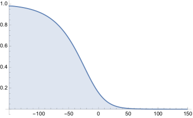
Figure 1.1. Plot of the cutoff profile $\varphi\big{(}2^{-\lambda}\big{)}$ for $\lambda\in[-150,150]$.

1.2. Continuous time dynamics

We turn to the analysis of the continuous time version of nonlinear recombinations. Given an initial state $\mu\in\mathcal{P}(\Omega)$, we define $S_{t}(\mu)\in\mathcal{P}(\Omega)$, $t\geq 0$, by the differential equation

$$\frac{d}{dt}\,S_{t}(\mu)=S_{t}(\mu)\circ S_{t}(\mu)\,-\,S_{t}(\mu)\,,\qquad S_{0}(\mu)=\mu,$$ (1.15)

where the symbol ‘$\circ$’ is defined by the averaged uniform recombination in (1.1). It can be checked that for each $\mu\in\mathcal{P}(\Omega)$ there exists a unique solution to the above Cauchy problem, see e.g. [1] for more general statements in this direction. We will actually provide an explicit construction of such a solution. Thus, equation (1.15) defines a nonlinear semigroup acting on $\mathcal{P}(\Omega)$: $S_{0}={\rm Id}$, $S_{t+s}=S_{t}S_{s}=S_{s}S_{t}$, for all $t,s\geq 0$, which is the natural continuous time analog of the semigroup $T_{t}$, $t\in{\mathbb{N}}$, defined in (1.2).

We stress, however, that in contrast with linear Markov chains, the continuous time evolution here cannot be obtained by a simple randomization of the number of steps taken by the discrete time dynamics. This is due to the fact that the collision product defined by (1.1) does not have the associative property. For instance, in general one has

$$(\mu\circ\mu)\circ(\mu\circ\mu)\neq((\mu\circ\mu)\circ\mu)\circ\mu.$$

Therefore, the “collision history”, not only the number of collisions, affects the final distribution. In fact, as we will see, solutions to the continuous time equation (1.15) admit an explicit representation in terms of a growing random binary rooted tree $\{\mathcal{T}_{t},t>0\}$, which records the history of all collisions contributing to the final state. This is equivalent to the classical representation of the solution of the Boltzmann equation in terms of Wild sums and McKean trees [5, 15, 16, 21]. The continuous model displays a behavior which is quite different from the discrete one: the value of the mixing time as well as the shape of the profile of convergence to equilibrium are changed.

As in the discrete time model, one has the convergence

$$S_{t}(\mu)\longrightarrow\pi_{\mu},\qquad t\to\infty,$$ (1.16)

to the product measure $\pi_{\mu}$ with the same marginals as the initial state $\mu$. Quantitative bounds for the speed of convergence have been obtained for the relative entropy and for the total variation distance [2, 3]. In particular, for any $\mu\in\mathcal{P}(\Omega)$ one has

$$\|S_{t}(\mu)-\pi_{\mu}\|_{\rm TV}\leq\tfrac{1}{2}\,n(n-1)\,e^{-t/2},\qquad t>0,$$ (1.17)

see Remark 3.4. Thus, a time $t=4\log n+O(1)$ is sufficient to achieve a small TV distance, regardless of the initial state. Here, we prove that the optimal location is actually $2\log n$ and show that the dynamics displays a cutoff phenomenon. Again, for simplicity, we restrict to balanced initial states $\mu\in\mathcal{B}_{n}$, and define

$$d_{n}(t):=\max_{\mu\in\mathcal{B}_{n}}\|S_{t}(\mu)-\pi\|_{\rm TV},$$ (1.18)

where $\pi$ is the uniform distribution over $\Omega$.

Theorem 1.3.

There exist a constant $c>0$ such that, for all integer $n\geq 1$ and all $t>0$, setting $r:=ne^{-t/2}$, one has

$$d_{n}(t)\leq r$$ (1.19)

$$d_{n}(t)\geq 1-2\exp\left(-c\min(\sqrt{r(1\vee\log(1/t))},n)\right)$$ (1.20)

In particular, if $t_{n,\lambda}:=2\log n+\lambda$, with $\lambda\in{\mathbb{R}}$, then

$$\lim_{\lambda\to\infty}\limsup_{n\to\infty}d_{n}(t_{n,\lambda})=0$$ (1.21)

$$\lim_{\lambda\to-\infty}\liminf_{n\to\infty}d_{n}(t_{n,\lambda})=1$$ (1.22)

We remark that (1.19) is entirely analogous to the upper bound in discrete time (1.8). On the other hand, the lower bound (1.20), which is in some sense optimal as discussed in Remark 3.8, displays a different asymptotics with respect to (1.9). Moreover, we note that the logarithmic term in $1/t$ in the exponent allows us to capture some nontrivial behavior for the time window $t\in(0,1)$ during which $d_{n}(t)$ drops from $1-2^{-n}$ to $1-e^{-\Theta(\sqrt{n})}$.

As for the analog of Theorem 1.2, we obtain the following cutoff profile in the case of monochromatic initial states. In analogy with (1.12), we write $\bar{d}_{n}(t)$ for the distance to stationarity when $\mu=\frac{1}{2}\mathbf{1}_{-}+\frac{1}{2}\mathbf{1}_{+}$.

Theorem 1.4.

If $t_{n,\lambda}=2\log n+\lambda$, with $\lambda\in{\mathbb{R}}$, then $\bar{d}_{n}(\cdot)$ satisfies

$$\lim_{n\to\infty}\bar{d}_{n}(t_{n,\lambda})=f(\lambda)\,,$$ (1.23)

where $f:\mathbb{R}\mapsto[0,1]$ is a decreasing continuous function with $f(\lambda)\to 1$, as $\lambda\to-\infty$, and $f(\lambda)\to 0$, as $\lambda\to\infty$.

As we will see, the function $f$ appearing in Theorem 1.4 admits the following more explicit representation: there exists a positive random variable $W$, with expected value $\mathbf{E}[W]=1$, such that

$$f(\lambda)=\big{\|}\mathcal{N}(0,1)-\mathbf{E}\big{[}\mathcal{N}(0,1+e^{-\lambda/2}W)\big{]}\big{\|}_{\rm TV},$$ (1.24)

that is $f(\lambda)$ is the total variation distance between the standard normal and a mixture of normal distributions, defined as the expected value of the centered normal with random variance $1+e^{-\lambda/2}W$. Note that if $W$ is replaced deterministically by $1$, then one recovers the profile $\varphi(e^{-\lambda/2})$, a rescaled version of the discrete time result in Theorem 1.2. In a sense, the random variable $W$ serves as a witness to the presence of additional randomness within the collision history in the continuous time setting, see Proposition 3.9.

We conclude this introduction with some of the ideas involved in the proofs of the results presented so far, and with some further comments and open questions.

1.3. Ideas of proof, comments, and open problems

We start with the observation that, in discrete time, by the definitions (1.1) and (1.2), $\mu_{t}=T_{t}(\mu)$ can be viewed graphically as the average of the distribution at the root of a rooted regular binary tree with depth $t$, where each internal node represents a random collision and the $2^{t}$ leaves of the tree are assigned i.i.d. samples from $\mu$, which we denote by $\xi=\{\xi(x),\,x=1,\dots,2^{t}\}$, and the distribution at each internal node $u$ is computed as the collision product of the two distributions at the children of $u$. Indeed, the case $t=1$ was discussed after (1.1), and the case of general $t$ is obtained by recursion, see Lemma 2.1. Thus we write $\mu_{t}={\mathbb{E}}[\mu_{t}^{\xi}]$, where $\mu^{\xi}_{t}$ is the conditional distribution at the root given the realization $\xi$. Equivalently, we view $\xi$ as a random environment, and the measure $\mu^{\xi}_{t}$ as a quenched distribution. By convexity, an upper bound is obtained by estimating the TV distance by the average of the quenched $L^{2}$ norm:

$$\|\mu_{t}-\pi\|_{\rm TV}=\tfrac{1}{2}\,\|{\mathbb{E}}\,(h^{\xi}_{t}-1)\|_{L^{1}(\pi)}\leq\tfrac{1}{2}\,{\mathbb{E}}\,\|\hat{h}^{\xi}_{t}-1\|_{L^{2}(\pi)}\,,$$ (1.25)

where $h^{\xi}_{t}=\,\text{\rm d}\mu^{\xi}_{t}/\,\text{\rm d}\pi$ is the relative density, $\hat{h}^{\xi}_{t}=h^{\xi}_{t}+g^{\xi}$ for any function $g^{\xi}$ such that ${\mathbb{E}}[g^{\xi}]=0$, and $\|\cdot\|_{L^{p}(\pi)}$ denotes the norm in $L^{p}(\Omega,\pi)$. The proof of the upper bound in Theorem 1.1 then proceeds with an estimation of the quenched $L^{2}$ norm featuring in (1.25), which in turn is obtained by an expansion of the shifted density $\hat{h}^{\xi}_{t}$ for a suitable choice of $g^{\xi}$.

Before discussing the proof of the lower bound in Theorem 1.1, it is convenient to address first the profile result in Theorem 1.2. The proof of this is based on showing that for the monochromatic $\mu$, if $\sigma\in\Omega$ is uniformly distributed, then $h(\sigma)=\mu_{t}(\sigma)/\pi(\sigma)$, the density of $\mu_{t}$ with respect to $\pi$, is well approximated, as $n\to\infty$ and $n2^{-t}\to s$, by the random variable

$$\frac{1}{\sqrt{s+1}}\,\exp{\left(\frac{s\big{(}\sum_{i=1}^{n}\sigma_{i}\big{)}^{2}}{2n(s+1)}\right)}.$$ (1.26)

Once this is achieved, the representation in terms of normal random variables appearing in (1.14) follows by using the CLT to replace $(\sum_{i}\sigma_{i})^{2}/n$ by the square of a standard normal.

The function $\varphi(s)$ in Theorem 1.2 satisfies $\varphi(s)=\frac{s}{\sqrt{2e\pi}}+o(s)$ as $s\to 0$, see Appendix A. This shows that the upper bound (1.8) captures the optimal linear dependence in $s$, as $s$ becomes small. On the other hand, $1-\varphi(s)=\frac{\sqrt{\log s}}{\sqrt{2\pi s}}(1+o(1))$ as $s\to\infty$, see again Appendix A. Therefore, the lower bound (1.9) cannot be achieved by the monochromatic distribution $\mu$ when $s$ is large. Indeed, the proof of the lower bound in Theorem 1.1 will use an initial condition $\mu$ consisting of a suitable product of monochromatic distributions on distinct blocks, which achieves a better lower bound than the monochromatic distribution on a single block. The analysis for this product measure is based on the detailed knowledge of the monochromatic case gathered within the proof of Theorem 1.2.

The strategy of proof in the continuous time setting is similar, with the crucial difference that in the graphical construction mentioned above the deterministic binary tree must be replaced by a random binary tree $\mathcal{T}_{t}$ encoding the collision history. The tree $\mathcal{T}_{t}$ can be defined, recursively, as follows: at time zero there is only one node, the root; after an exponentially distributed random time with mean $1$, the root gives rise to two new particles; independently, each newly created particle repeats the same random splitting, and so on. $\mathcal{T}_{t}$ represents the resulting random tree at time $t$, and the distribution $S_{t}(\mu)$ is calculated as an average over the realization of $\mathcal{T}_{t}$ of the distribution obtained at the root when each internal node is assigned the distribution given by the collision product of the distributions assigned to its two children, and the leaves are assigned the distribution $\mu$, see Lemma 3.1. We let $L(\mathcal{T}_{t})$ denote the set of leaves of $\mathcal{T}_{t}$ and write $|x|$ for the depth of a leaf $x\in L(\mathcal{T}_{t})$, which is defined as the number of splittings along the path from the root to $x$. An important role in the analysis of the continuous time dynamics is played by the process defined as

$$W_{t}=e^{t/2}\sum_{x\in L(\mathcal{T}_{t})}4^{-|x|}\,,\qquad t\geq 0.$$ (1.27)

Using size-biasing, and a spinal representation in the spirit of [6, 10, 14], the process $W_{t}$ will be shown to define a uniformly integrable martingale, converging to a positive random variable $W_{\infty}$ with mean $\mathbf{E}[W_{\infty}]=1$. In a sense that will be made more precise by our results later on, one can say that the order parameter $s=n2^{-t}$, governing the cutoff transition in the discrete time dynamics, must be replaced in the continuous time setting by the random variable

$$ne^{-t/2}W_{t}\,\longrightarrow\,rW_{\infty}.$$

In particular, the random variable $W$ appearing in the limiting profile function in Theorem 1.4 is precisely $W_{\infty}$.

As anticipated, there are no conceptual difficulties in extending our cutoff result to more general settings where balanced distributions $\mu\in\mathcal{B}_{n}$ are replaced by arbitrary probability distributions $\mu$ on $\Omega$, provided that one assumes that the family of measures $\mu$ considered is such that the marginals $\mu(\sigma_{i}=1)$ are uniformly bounded away from $0$ and $1$. We give some more detailed comments in Section 2.5 below. Moreover, we believe that a cutoff phenomenon should continue to hold even for more general state spaces, that is when $\Omega=\{-1,+1\}^{n}$ is replaced by ${\mathbb{X}}^{n}$, with ${\mathbb{X}}$ a generic finite alphabet, and all marginals are assumed to be uniformly nondegenerate.

Finally, let’s address some open questions that naturally emerge from the preceding discussion. A first question concerns the existence of a cutoff phenomenon for nonlinear recombinations where the uniform choice of $A$ in the single recombination step (1.1) is replaced by a more general distribution $\nu$ over subsets of $[n]$. The speed of convergence in such models can be related to the probability, under $\nu$, of separating any two given sites at each step, which gives the natural analog of (1.4) and (1.17), see [17] for the discrete time, and [2] for the continuous time. We believe that a cutoff phenomenon should occur for such cases as well, but our proofs make explicit use of the uniformity in (1.1). A second problem concerns the analysis of more general quadratic systems with nontrivial interactions in the stationary distribution, see [3, 18] for the definition of a general framework for quadratic reversible dynamical systems in combinatorial settings. A particular example is the nonlinear dynamics for Ising systems, obtained by a modification of the one step recombination (1.1) where the content swap on the set $A$ is accepted or rejected, in such a way that the dynamics converges to the Ising distribution on a given interaction graph. This may be seen as a nonlinear version of the usual Metropolis algorithm. In the high-temperature regime, tight bounds on the speed of convergence for these models were recently derived [4]. Drawing an analogy with the known cutoff results for high-temperature spin systems [13], we conjecture a similar cutoff phenomenon in the nonlinear version as well.

2. Discrete time

We start with a representation of the distribution $\mu_{t}=T_{t}(\mu)$ at time $t\in{\mathbb{N}}$, valid for any $\mu\in\mathcal{P}(\Omega)$. This representation is convenient since it provides, conditionally given some random environment $\xi$ to be defined below, an independence between the $n$ bits.

2.1. Graphical construction and fragmentation

By definition, the solution $\mu_{t}=T_{t}(\mu)$, of the dynamical system (1.2) admits the following simple graphical interpretation. Consider the rooted regular binary tree with depth $t$, and assign to each node $u$ a distribution $\nu_{u}\in\mathcal{P}(\Omega)$ in such a way that each of the $2^{t}$ leaves is assigned the distribution $\mu$ and the distribution at each internal node $u$ is computed as the collision product of the two distributions at the children of $u$. Then $\mu_{t}$ is the distribution at the root of the tree, see Figure 2.1 for the case $t=2$.

Figure 2.1. $T_{2}(\mu)$ is the distribution at the root of the binary tree with depth $2$.

It is useful to have a pathwise implementation of this graphical construction. Set $N:=2^{t}$, and let $\xi(1),\dots,\xi(N)$ denote $N$ independent random variables with law $\xi(x)\sim\mu$ for every leaf $x\in\{1,\ldots,N\}$. Define

$$q^{\xi}(i):=\frac{1}{N}\sum_{x=1}^{N}\xi_{i}(x),\qquad i\in[n],$$ (2.1)

where $\xi_{i}(x)\in\{-1,+1\}$ denotes the $i$-th bit in the string $\xi(x)\in\Omega$. The next lemma expresses $\mu_{t}$ as an average ${\mathbb{E}}[\mu_{t}^{\xi}]$, where ${\mathbb{E}}$ denotes the expectation w.r.t. the random variables $\xi=\{\xi(x),\,x=1,\dots,N\}$, and the quenched measure $\mu_{t}^{\xi}$ is a product of $n$ Bernoulli random variables each with marginal

$$\mu_{t}^{\xi}(\sigma_{i}=\pm 1)=(1\pm q^{\xi}(i))/2.$$

Lemma 2.1.

For any $\mu\in\mathcal{P}(\Omega)$, we have $\mu_{t}={\mathbb{E}}[\mu_{t}^{\xi}]$, where

$$\mu^{\xi}_{t}(\sigma)=2^{-n}\prod_{i=1}^{n}(1+\sigma_{i}q^{\xi}(i)).$$ (2.2)

Proof.

We start by observing that for every $t\in{\mathbb{N}}$, $\mu\in\mathcal{P}(\Omega)$,

$$\mu_{t}=\frac{1}{N^{n}}\sum_{\begin{subarray}{c}(A_{1},\dots,A_{N}):\\ \sqcup A_{i}=[n]\end{subarray}}\mu_{A_{1}}\otimes\mu_{A_{2}}\otimes\dots\otimes\mu_{A_{N}},$$ (2.3)

where the sum is taken over all partitions of $[n]$ into $N=2^{t}$ disjoint sets (which are allowed to be empty). The case $t=1$ is just the definition of uniform recombination (1.1) and the case $t\geq 2$ follows by induction since if $(A_{1},\dots,A_{N})$, $(A^{\prime}_{1},\dots,A^{\prime}_{N})$ are two independent uniformly random partitions of $[n]$ into $N$ disjoint sets, and $A\subset[n]$ is taken independently and uniformly at random, then

$$(A_{1}\cap A,\dots,A_{N}\cap A,A^{\prime}_{1}\cap A^{c},\dots,A^{\prime}_{N}\cap A^{c})$$ (2.4)

yields a uniformly random partition of $[n]$ into $2N$ disjoint sets.

A way to sample such a partition uniformly at random amongst the $N^{n}$ possibilities is to assign to each $i\in[n]$ independently a uniformly random number $U_{i}$ in $[N]=\{1,\dots,N\}$ and define

$$A_{x}:=\{i\in[n]\ :U_{i}=x\},\qquad x=1,\dots,N.$$ (2.5)

We denote the associated probability by $P$, and write $E$ for the corresponding expectation. With this definition, (2.3) becomes

$$\mu_{t}=E\left[\mu_{A_{1}}\otimes\mu_{A_{2}}\otimes\dots\otimes\mu_{A_{N}}\right].$$ (2.6)

Thus, if $\xi(x)=(\xi_{1}(x),\dots,\xi_{n}(x))$, $x\in[N]$, are IID with distribution $\mu$, then for any $\sigma\in\Omega$, using Fubini Theorem

$$\begin{split}\mu_{t}(\sigma)&=\textstyle{E\left[\prod_{x=1}^{N}\mu_{A_{x}}(\sigma_{A_{x}})\right]}\\ &=E\left[{\mathbb{P}}\left[\forall x\in[N],\ \forall i\in A_{x},\ \xi_{i}(x)=\sigma_{i}\right]\right]\\ &={\mathbb{E}}\left[P\left[\forall x\in[N],\ \forall i\in A_{x},\ \xi_{i}(x)=\sigma_{i}\right]\right]\\ &={\mathbb{E}}\left[P\left[\forall i\in[n],\ \xi_{i}(U_{i})=\sigma_{i}\right]\right].\end{split}$$ (2.7)

Therefore, $\mu_{t}={\mathbb{E}}[\mu^{\xi}_{t}]$, where the quenched probability $\mu^{\xi}_{t}$ coincides with the distribution of $(\xi_{i}(U_{i}))^{n}_{i=1}$ given $\xi$. Since, conditionally on $\xi$, the $\xi_{i}(U_{i})$, $i\in[n]$, are independent and $\xi_{i}(U_{i})=\pm 1$ with probability $(1\pm q^{\xi}(i))/2$, this proves (2.2). ∎

The above lemma can be summarized as follows. If each leaf $x\in[N]$ is assigned the configuration $\xi(x)$, where the $(\xi(x))$ are IID with law $\mu$ and each $i\in[n]$ is assigned the leaf $U_{i}$, where the $(U_{i})$ are IID uniform in $[N]$, then the configuration at the root given by $\sigma=(\xi_{1}(U_{1}),\dots,\xi_{n}(U_{n}))$ has law $\mu_{t}$. Conditionally on the variables $(U_{i})$ the vector $\sigma$ has the law $\mu_{A_{1}}\otimes\dots\otimes\mu_{A_{N}}$, where the subsets $A_{x}$ are given in (2.5). The partition $(A_{x})$ can be seen as the result of a fragmentation of the set $[n]$ at time $t$. More precisely, we define a discrete time fragmentation process $\mathcal{A}_{t}$ such that $\mathcal{A}_{0}=[n]$, and if $\mathcal{A}_{t}=(A_{x})^{2^{t}}_{x=1}$, then $\mathcal{A}_{t+1}=(A^{\prime}_{y})^{2^{t+1}}_{y=1}$ is obtained by replacing each $A_{x}$ by the two sets $A_{x}\cap A$ and $A_{x}\cap A^{c}$ , where $A$ is a uniformly random subset of $[n]$. Note that at each time $t$ this gives a uniformly random partition of $[n]$ into $N=2^{t}$ subsets. We may define the fragmentation time $\tau_{\rm frag}$ as the first time $t$ such that all subsets in $\mathcal{A}_{t}$ are either empty or a singleton. This coincides with the first time such that for all indexes $1\leq i<\ell\leq n$, one has $i$ and $\ell$ in different subsets of the partition. By the above construction one sees that conditionally on $\{\tau_{\rm frag}\leq t\}$, the random vector $\sigma$ at the root at time $t$ is a product of independent bits, and is thus distributed according to $\pi_{\mu}$. It follows that

$$\|\mu_{t}-\pi\|_{\rm TV}\leq{\mathbb{P}}(\tau_{\rm frag}>t)\leq\tfrac{1}{2}n(n-1)2^{-t}\,,$$ (2.8)

where we use a union bound over pairs $1\leq i<\ell\leq n$ and the fact that for a given such pair, the probability to have $i$ and $\ell$ in the same set of the partition $\mathcal{A}_{t}$ at time $t$ is exactly $2^{-t}$. Moreover, it is not hard to see that $\tau_{\rm frag}$ is actually concentrated around $2\log_{2}n$, that is the function $t\mapsto{\mathbb{P}}(\tau_{\rm frag}>t)$ has a cutoff behavior at $t=2\log_{2}n$ with an $O(1)$ window.

2.2. Upper bound for discrete time

We provide now a better strategy, which allows us to prove the upper bound (1.8) on the TV distance. This improves the bound given in (2.8) by a factor $n$, thus achieving the optimal bound $\log_{2}n+O(1)$ for the cutoff time. The next lemma establishes the upper bound in Theorem 1.1.

Lemma 2.2.

For every $n,t\in{\mathbb{N}}$, for all $\mu\in\mathcal{B}_{n}$,

$$\|\mu_{t}-\pi\|_{\rm TV}\leq n2^{-t}\;.$$ (2.9)

Proof.

From Lemma 2.1 we have $\mu_{t}={\mathbb{E}}[\mu_{t}^{\xi}]$, where $\mu_{t}^{\xi}\in\mathcal{P}(\Omega)$ has density

$$h^{\xi}_{t}(\sigma)=\frac{\,\text{\rm d}\mu^{\xi}_{t}}{\,\text{\rm d}\pi}(\sigma)=\prod_{i=1}^{n}(1+\sigma_{i}q^{\xi}(i)).$$ (2.10)

Using ${\mathbb{E}}\left[q^{\xi}(i)\right]=0$ for all $i\in[n]$, we obtain

$$\|\mu_{t}-\pi\|_{\rm TV} =\tfrac{1}{2}\,\|{\mathbb{E}}\,(h^{\xi}_{t}-1)\|_{L^{1}(\pi)}$$

$$=\tfrac{1}{2}\,\textstyle{\|{\mathbb{E}}\,(h^{\xi}_{t}-\sum^{n}_{i=1}\sigma_{i}q^{\xi}(i)-1)\|_{L^{1}(\pi)}}$$

$$\leq\tfrac{1}{2}\,\textstyle{{\mathbb{E}}\,\|h^{\xi}_{t}-\sum^{n}_{i=1}\sigma_{i}q^{\xi}(i)-1\|_{L^{1}(\pi)}}\,.$$ (2.11)

On the one hand, using at the last line that $\sigma_{i}$ are IID centered r.v. under $\pi$

$$\textstyle{\|h^{\xi}_{t}-\sum^{n}_{i=1}\sigma_{i}q^{\xi}(i)-1\|_{L^{1}(\pi)}}$$ (2.12)

$$\qquad\leq\int h^{\xi}_{t}d\pi+1+\int\textstyle{\left|\sum^{n}_{i=1}\sigma_{i}q^{\xi}(i)\right|d\pi}$$ (2.13)

$$\qquad\leq 2+\left(\int\textstyle{\left(\sum_{i=1}^{n}\sigma_{i}q^{\xi}(i)\right)^{2}\,\text{\rm d}}\pi\right)^{1/2}=2+\textstyle{\langle q^{\xi},q^{\xi}\rangle^{1/2}}\;,$$ (2.14)

where we use the notation $\langle x,y\rangle=\sum_{i=1}^{n}x(i)y(i)$. On the other hand, writing $\hat{h}^{\xi}_{t}=h^{\xi}_{t}-\sum^{n}_{i=1}\sigma_{i}q^{\xi}(i)$, we estimate

$$\textstyle{\|h^{\xi}_{t}-\sum^{n}_{i=1}\sigma_{i}q^{\xi}(i)-1\|^{2}_{L^{1}(\pi)}} \leq\|\hat{h}^{\xi}_{t}-1\|^{2}_{L^{2}(\pi)}=\int\left(\hat{h}^{\xi}_{t}\right)^{2}\!\,\text{\rm d}\pi\,-\,1$$ (2.15)

$$=\prod_{i=1}^{n}\left(1+q^{\xi}(i)^{2}\right)-\sum^{n}_{i=1}q^{\xi}(i)^{2}-1$$ (2.16)

$$\leq e^{\langle q^{\xi},q^{\xi}\rangle}-\langle q^{\xi},q^{\xi}\rangle-1\;.$$ (2.17)

Using the inequality

$$\min\left\{\left(e^{\langle q^{\xi},q^{\xi}\rangle}-\langle q^{\xi},q^{\xi}\rangle-1\right)^{1/2},2+\langle q^{\xi},q^{\xi}\rangle^{1/2}\right\}\leq 2\langle q^{\xi},q^{\xi}\rangle\;,$$ (2.18)

we have thus shown that

$$\|\mu_{t}-\pi\|_{\rm TV}\leq{\mathbb{E}}\left[\langle q^{\xi},q^{\xi}\rangle\right]=n{\mathbb{E}}\left[(q^{\xi}(1))^{2}\right]=n2^{-t}\,.$$ (2.19)

∎

The previous result establishes an upper bound on $D_{n}(t)$ which, for large $t$ or equivalently for small $s=n2^{-t}$, is asymptotically sharp up to constant (cf. the discussion in Section 1.3 or Section 2.4 below). However it does not yield any information about the case $t$ small or equivalently $s$ large. The following lemma fills this gap by providing a bound, which captures the decay of the distance to equilibrium at times $t=\log_{2}n-K$ for large constants $K$. It is in a sense quite close to the asymptotic lower bound (1.9) which we will obtain in Section 2.4, as the two only differ by the constant that appears in the exponential.

Lemma 2.3.

For every $n,t\in{\mathbb{N}}$, setting $s:=n2^{-t}$, and for all $\mu\in\mathcal{B}_{n}$,

$$\|\mu_{t}-\pi\|_{\rm TV}\leq 1-\tfrac{1}{2}\,e^{-2s},\qquad s\geq\log(2)/2.$$ (2.20)

Proof.

We proceed as in the previous proof but instead of using only Schwarz’ inequality to bound the $L^{1}(\pi)$ norm by the $L^{2}(\pi)$ norm, we use the following finer inequality, whose proof is given in Appendix B, namely

$$\tfrac{1}{2}\,\|f-1\|_{L^{1}(\pi)}\leq\phi\left(\|f-1\|_{L^{2}(\pi)}\right),$$ (2.21)

with

$$\phi(x)=\begin{cases}x/2,&\text{ if }x\leq 1,\\ \frac{x^{2}}{1+x^{2}}\quad&\text{ if }x\geq 1.\end{cases}$$

Note that

$$\|h^{\xi}_{t}-1\|^{2}_{L^{2}(\pi)}=\int\left(h^{\xi}_{t}\right)^{2}\!\,\text{\rm d}\pi\,-\,1=\prod_{i=1}^{n}\left(1+q^{\xi}(i)^{2}\right)-1\leq e^{\langle q^{\xi},q^{\xi}\rangle}-1.$$ (2.22)

Using monotonicity of $\phi$ and (2.21),

$$\|\mu_{t}-\pi\|_{\rm TV}\leq{\mathbb{E}}\left[\phi\left(\sqrt{e^{\langle q^{\xi},q^{\xi}\rangle}-1}\,\right)\right].$$ (2.23)

Moreover, ${\mathbb{E}}\left[\langle q^{\xi},q^{\xi}\rangle\right]=n2^{-t}=s$, and therefore, by Markov’s inequality,

$${\mathbb{P}}\left(\langle q^{\xi},q^{\xi}\rangle\geq 2s\right)\leq\frac{1}{2}\,.$$

Since $\phi$ is non-decreasing and bounded by $1$, and provided $2s\geq\log 2$, we obtain

$$\|\mu_{t}-\pi\|_{\rm TV} \leq{\mathbb{E}}\left[\mathbf{1}_{\langle q^{\xi},q^{\xi}\rangle\geq 2s}+(1-\mathbf{1}_{\langle q^{\xi},q^{\xi}\rangle\geq 2s})\phi\left(\sqrt{e^{2s}-1}\,\right)\right]$$

$$\leq{\mathbb{P}}\big{(}\langle q^{\xi},q^{\xi}\rangle\geq 2s\big{)}+\big{(}1-{\mathbb{P}}\big{(}\langle q^{\xi},q^{\xi}\rangle\geq 2s\big{)}\big{)}(1-e^{-2s})$$

$$\leq 1-\tfrac{1}{2}\,e^{-2s}.$$

∎

2.3. Explicit profile for monochromatic initial states

Here we prove Theorem 1.2. We take the monochromatic distribution $\mu=\tfrac{1}{2}\,\mathbf{1}_{-}+\tfrac{1}{2}\,\mathbf{1}_{+}$ as initial state. Using the notation from Lemma 2.1, we note that now $q^{\xi}(i)$ does not depend on $i$. We let $\bar{q}^{\xi}$ denote this common value, and write $\rho_{t}$ for the probability density

$$\rho_{t}(\sigma)=\frac{\,\text{\rm d}\mu_{t}}{\,\text{\rm d}\pi}(\sigma)={\mathbb{E}}\left[h^{\xi}_{t}\right]={\mathbb{E}}\left[\prod_{i=1}^{n}(1+\sigma_{i}\bar{q}^{\xi})\right].$$ (2.24)

Proposition 2.4.

If $t_{n}\in{\mathbb{N}}$ is such that $\lim_{n\to\infty}n2^{-t_{n}}=s$ for some $s>0$, then for any bounded continuous function $F:{\mathbb{R}}_{+}\mapsto{\mathbb{R}}$,

$$\lim_{n\to\infty}\int F(\rho_{t_{n}}(\sigma))\pi(\,\text{\rm d}\sigma)=\int\frac{e^{-\frac{z^{2}}{2}}}{\sqrt{2\pi}}\,F\left(\gamma_{s}(z)\right)\,\text{\rm d}z,$$ (2.25)

with

$$\gamma_{s}(z):=\frac{e^{\frac{sz^{2}}{2(s+1)}}}{\sqrt{s+1}}\;,\quad z\in\mathbb{R}\;.$$ (2.26)

The asserted convergence can be interpreted as convergence in distribution of $\rho_{t_{n}}$ viewed as a r.v. on $(\Omega,\pi)$ towards $\gamma_{s}$ viewed as a r.v. on $(\mathbb{R},\mathcal{N}(0,1))$. As a consequence, we can restrict ourselves to smoother functions $F$ in the proof (we will take Lipschitz bounded functions).

Let us first observe that Proposition 2.4 implies Theorem 1.2.

Proof of Theorem 1.2.

By definition (1.13) and since $\gamma_{s}$ is the relative density of $\mathcal{N}(0,1+s)$ with respect to $\mathcal{N}(0,1)$, one has

$$\varphi(s)=\|\mathcal{N}(0,1+s)-\mathcal{N}(0,1)\|_{{\rm TV}}=\frac{1}{2}\int\frac{e^{-\frac{z^{2}}{2}}}{\sqrt{2\pi}}\left|\gamma_{s}(z)-1\right|\,\text{\rm d}z.$$

Thus, we need to prove that for $t_{n}\in{\mathbb{N}}$ such that $\lim_{n\to\infty}n2^{-t_{n}}=s$,

$$\begin{split}\lim_{n\to\infty}\int\left|\rho_{t_{n}}(\sigma)-1\right|\pi(\,\text{\rm d}\sigma)=\int\frac{e^{-\frac{z^{2}}{2}}}{\sqrt{2\pi}}\left|\gamma_{s}(z)-1\right|\,\text{\rm d}z.\end{split}$$ (2.27)

Since the map $F:x\mapsto 1+x-|x-1|$ is bounded and continuous on $\mathbb{R}_{+}$, Proposition 2.4 yields

$$\lim_{n\to\infty}\int\left[(1+\rho_{t_{n}}(\sigma))-|\rho_{t_{n}}(\sigma)-1|\right]\pi(\,\text{\rm d}\sigma)$$ (2.28)

$$\qquad\qquad=\int\frac{e^{-\frac{z^{2}}{2}}}{\sqrt{2\pi}}\left[\left(1+\gamma_{s}(z)\right)-\left|\gamma_{s}(z)-1\right|\right]\,\text{\rm d}z.$$ (2.29)

Since $\int(1+\rho_{t_{n}}(\sigma))\pi(\,\text{\rm d}\sigma)=2=\int\frac{e^{-\frac{z^{2}}{2}}}{\sqrt{2\pi}}\left(1+\gamma_{s}(z)\right)\,\text{\rm d}z$, (2.27) follows. ∎

Proof of Proposition 2.4.

Without loss of generality, we can assume $F$ Lipschitz and bounded. To prove (2.25) we are going to show that $\rho_{t_{n}}(\sigma)$ is well approximated by

$$\gamma_{s}(\bar{\sigma}_{n})=\frac{e^{\frac{s\,\bar{\sigma}_{n}^{2}}{2(s+1)}}}{\sqrt{s+1}},\qquad\bar{\sigma}_{n}:=\frac{1}{\sqrt{n}}\sum_{i=1}^{n}\sigma_{i}\,.$$ (2.30)

That is, we show that

$$\lim_{n\to\infty}\int\left|F(\rho_{t_{n}}(\sigma))-F(\gamma_{s}(\bar{\sigma}_{n}))\right|\pi(\,\text{\rm d}\sigma)=0.$$ (2.31)

Once (2.31) is available, it is sufficient to prove (2.25) with $\rho_{t_{n}}(\sigma)$ replaced by $\gamma_{s}(\bar{\sigma}_{n})$, that is

$$\lim_{n\to\infty}\int F(\gamma_{s}(\bar{\sigma}_{n}))\pi(\,\text{\rm d}\sigma)=\int\frac{e^{-\frac{z^{2}}{2}}}{\sqrt{2\pi}}\,F\left(\gamma_{s}(z)\right)\,\text{\rm d}z.$$ (2.32)

However, since $F\circ\gamma_{s}$ is bounded and continuous, the above convergence follows simply from the fact that $\bar{\sigma}_{n}$ converges in distribution, under $\pi$, to a standard Gaussian.

We are left with the proof of (2.31). Observing that

$$\prod_{i=1}^{n}(1+\sigma_{i}\bar{q}^{\xi})^{2}=(1+\bar{q}^{\xi})^{\sqrt{n}{\bar{\sigma}_{n}}}(1-\bar{q}^{\xi})^{-\sqrt{n}{\bar{\sigma}_{n}}}\left(1-(\bar{q}^{\xi})^{2}\right)^{n},$$

one has

$$\rho_{t_{n}}(\sigma)={\mathbb{E}}\left[e^{\alpha_{n}^{\xi}\bar{\sigma}_{n}+\beta_{n}^{\xi}}\right],$$ (2.33)

where

$$\alpha_{n}^{\xi}:=\frac{\sqrt{n}}{2}\log\left(\frac{1+\bar{q}^{\xi}}{1-\bar{q}^{\xi}}\right),\quad\beta_{n}^{\xi}:=\frac{n}{2}\log\left(1-(\bar{q}^{\xi})^{2}\right),$$ (2.34)

with adequate convention for the special case $\bar{q}^{\xi}=1$. The key observation for the proof is the following joint convergence in distribution

$$\lim_{n\to\infty}(\alpha^{\xi}_{n},\beta^{\xi}_{n})\stackrel{{\scriptstyle(d)}}{{=}}\left(Z_{s},-\frac{1}{2}Z_{s}^{2}\right),$$ (2.35)

where $Z_{s}\sim\mathcal{N}(0,s)$. Indeed, (2.35) is a direct consequence of an expansion of the logarithm in (2.34), using $n2^{-t_{n}}\to s$ and the convergence in distribution of

$$\sqrt{2^{t_{n}}}\bar{q}^{\xi}=\frac{1}{\sqrt{2^{t_{n}}}}\sum_{x=1}^{2^{t_{n}}}\xi_{1}(x)$$

to a standard gaussian.

If in (2.33) we replace formally the variables $\alpha_{n}^{\xi},\beta_{n}^{\xi}$ by their limits, then the computation of a gaussian integral gives the desired result, namely that $\rho_{t_{n}}$ is well approximated by (2.30). At this point, to conclude the proof there are two issues one has to consider: (a) we need more than convergence in distribution to replace $\alpha^{\xi}_{n}$ and $\beta^{\xi}_{n}$ in the expectation, (b) the fact that the space in which $\sigma$ lives depends on $n$ makes passing to the limit more tricky. Given $a\in{\mathbb{R}}$, we set

$$g_{n}(a,\bar{q}^{\xi}):=e^{\alpha_{n}^{\xi}a+\beta_{n}^{\xi}}.$$

Note that $\alpha_{n}^{\xi}$ and $\beta_{n}^{\xi}$ only depend on $\bar{q}^{\xi}$ so that this definition makes sense. Note the dependence on $n$ is also hidden in the fact that $\xi$ depends on $t=t_{n}$. An important observation is the following

Lemma 2.5.

If $\lim_{n\to\infty}n2^{-t_{n}}=s$, then for all $a\in{\mathbb{R}}$,

$$\lim_{n\to\infty}{\mathbb{E}}\left[g_{n}(a,\bar{q}^{\xi})\right]=\frac{1}{\sqrt{s+1}}e^{\frac{sa^{2}}{2(s+1)}}=\gamma_{s}(a),$$ (2.36)

and the convergence is uniform on the interval $a\in[-A,A]$ for any $A>0$.

The proof of Lemma 2.5 will be given below. We can now conclude the proof of (2.31). To that end, it suffices to show that for any given $A>0$

$$\limsup_{n\to\infty}\int\Big{|}F(\rho_{t_{n}}(\sigma))-F(\gamma_{s}(\bar{\sigma}_{n}))\Big{|}\mathbf{1}_{\{|\bar{\sigma}_{n}|\leq A\}}\pi(\,\text{\rm d}\sigma)=0\;,$$ (2.37)

and that

$$\lim_{A\to\infty}\limsup_{n\to\infty}\int\Big{|}F(\rho_{t_{n}}(\sigma))-F(\gamma_{s}(\bar{\sigma}_{n}))\Big{|}\mathbf{1}_{\{|\bar{\sigma}_{n}|>A\}}\pi(\,\text{\rm d}\sigma)=0\;.$$ (2.38)

We start with the latter. By Hoeffding’s inequality

$$\pi(\{|\bar{\sigma}_{n}|>A\})\leq 2e^{-A^{2}/2}\;,\quad A>0\;.$$

Since $F$ is bounded, we easily deduce (2.38).

On the other hand, since $\rho_{t_{n}}(\sigma)$ coincides with ${\mathbb{E}}\left[g_{n}(a,\xi)\right]$ evaluated at $a=\bar{\sigma}_{n}$, (2.37) follows from Lemma 2.5 and the fact that $F$ is Lipschitz. ∎

Proof of Lemma 2.5.

We claim that for any $A>0$,

$$\sup_{|a|\leq A}\sup_{n\geq 1}\max\left\{\|g_{n}(a,\cdot)\|_{\infty},\|\partial_{a}g_{n}(a,\cdot)\|_{\infty}\right\}<\infty$$ (2.39)

Indeed, computing the derivative in $\bar{q}^{\xi}$ of $g_{n}(a,\bar{q}^{\xi})$ shows that it is maximized at $\bar{q}^{\xi}=a/\sqrt{n}$ and from this, we deduce the bound on $\|g_{n}(a,\cdot)\|_{\infty}$. Regarding the bound on $\partial_{a}g_{n}(a,\cdot)$, we observe that $|\partial_{a}g_{n}(a,\bar{q}^{\xi})|\leq\max\{g_{n}(a+1,\bar{q}^{\xi});g_{n}(a-1,\bar{q}^{\xi})\}$.

As a consequence of the bound (2.39), we deduce that for $a\in[-A,A]$, the map $g_{n}(a,\cdot)$ coincides with $g_{n}(a,\cdot)\wedge M$ for some positive constant $M$. The latter is a continuous bounded function of $\alpha_{n}^{\xi}$ and $\beta_{n}^{\xi}$, so the convergence in law (2.35) implies that

$$\lim_{n\to\infty}{\mathbb{E}}\left[g_{n}(a,\bar{q}^{\xi})\right]={\mathbb{E}}\left[e^{aZ_{s}-\frac{1}{2}Z_{s}^{2}}\right]=\frac{1}{\sqrt{s+1}}e^{\frac{s\,a^{2}}{2(s+1)}}.$$ (2.40)

The bound on the derivative in $a$ of $g_{n}(a,\bar{q}^{\xi})$ proven above suffices to deduce that $a\mapsto{\mathbb{E}}\left[g_{n}(a,\bar{q}^{\xi})\right]$ is equicontinuous on $[-A,A]$. From this property, we deduce that the convergence (2.40) holds uniformly. ∎

We conclude with some remarks on the asymptotic behavior in the regime where $n2^{-t}\to\infty$. For instance, when $t\in{\mathbb{N}}$ is fixed one has the following behavior.

Lemma 2.6.

If $t\in{\mathbb{N}}$ is fixed, and $\mu=\frac{1}{2}\mathbf{1}_{+}+\frac{1}{2}\mathbf{1}_{-}$, then

$$\lim_{n\to\infty}\|\mu_{t}-\pi\|_{\rm TV}=1-\binom{2^{t}}{2^{t-1}}\,2^{-2^{t}}.$$ (2.41)

Proof.

From Lemma 2.1,

$$\|\mu_{t}-\pi\|_{\rm TV}\leq{\mathbb{E}}\left[\big{\|}\mu^{\xi}_{t}-\pi\big{\|}_{\rm TV}\right].$$ (2.42)

Since we are in the monochromatic case, under $\mu^{\xi}_{t}$, the $(\sigma_{i})$ are IID $\{-1,1\}$ valued Bernoulli variables with parameter $\frac{1+\bar{q}^{\xi}}{2}$. In particular $\mu^{\xi}_{t}=\pi$ if $\bar{q}^{\xi}=0$. Hence we have

$${\mathbb{E}}\left[\big{\|}\mu^{\xi}_{t}-\pi\big{\|}_{\rm TV}\right]\leq{\mathbb{P}}[\bar{q}^{\xi}\neq 0]=1-\binom{2^{t}}{2^{t-1}}\,2^{-2^{t}}.$$ (2.43)

In order to prove a matching lower bound, consider the event

$$A_{t}:=\textstyle{\left\{\left|\sum^{n}_{i=1}\sigma_{i}\right|\geq n2^{-t}\right\}}.$$

Then,

$$\|\mu_{t}-\pi\|_{\rm TV}\geq\mu_{t}(A_{t})-\pi(A_{t}) ={\mathbb{E}}\left[\mu^{\xi}_{t}(A_{t})\right]-\pi(A_{t})$$ (2.44)

$$\geq{\mathbb{E}}\left[\mathbf{1}_{\{\bar{q}^{\xi}\neq 0\}}(1-\mu^{\xi}_{t}(A_{t}^{c}))\right]-\pi(A_{t})\;.$$ (2.45)

By Hoeffding’s inequality, we know that $\pi(A_{t})\leq 2e^{-n2^{-2t}/2}$. On the other hand, note that $\bar{q}_{\xi}$ takes its values in the set $\{2k2^{-t}:k=-2^{t-1},\ldots,2^{t-1}\}$. Consequently, assuming $\bar{q}^{\xi}\neq 0$, we have $|\bar{q}^{\xi}|\geq 2^{1-t}$ and therefore Hoeffding’s inequality yields

$$\mu^{\xi}_{t}(A_{t}^{c})\leq\mu^{\xi}_{t}\left(|\textstyle{\sum^{n}_{i=1}}\sigma_{i}-n\bar{q}^{\xi}|\geq n2^{-t}\right)\leq 2e^{-n2^{-2t}/2}\;.$$ (2.46)

Hence we have

$$\|\mu_{t}-\pi\|_{\rm TV}\geq{\mathbb{P}}[\bar{q}^{\xi}\neq 0]-4e^{-n2^{-2t}/2},$$ (2.47)

which concludes our proof. ∎

Remark 2.7.

Lemma 2.6 shows in particular that the distance to equilibrium is far from being monotone for monochromatic initial states, see Figure 2.2. Indeed, in the limit of $n$ large, it drops from $1$ to $1/2$ in one step, it is macroscopically increasing during the first few subsequent steps and then it gradually increases to $1$ before entering the cutoff window $t_{n,\lambda}=\lfloor\log_{2}n+\lambda\rfloor$, $\lambda\in{\mathbb{R}}$, where it settles to the cutoff profile as stated in Theorem 1.2.

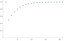
Figure 2.2. Plot of the function in the right hand side of (2.41) expressing the total variation distance after $t$ steps, started from the monochromatic distribution, in the limit $n\to\infty$.

Remark 2.8.

We observe that, with minor modifications, the argument in Lemma 2.6 can be extended to obtain the following statement: if $1\ll 2^{t}\ll\sqrt{n}$, then

$$\|\mu_{t}-\pi\|_{\rm TV}=1-\frac{1}{\sqrt{\pi 2^{t}}}(1+o(1)).$$ (2.48)

On the other hand, with a bit of extra work, the argument in the proof of Theorem 1.2, combined with the asymptotics $\varphi(s)=1-\frac{\sqrt{\log s}}{\sqrt{2\pi s}}(1+o(1))$, as $s\to\infty$, see Appendix A, can be seen to imply that if $\sqrt{n}\ll 2^{t}\ll n$, then we have

$$\|\mu_{t}-\pi\|_{\rm TV}=1-\frac{\sqrt{\log(n/2^{t})}}{\sqrt{2\pi(n/2^{t})}}(1+o(1))$$ (2.49)

2.4. Lower bound for discrete time

The lower bound we obtained in Theorem 1.2 for the monochromatic state is of order $s$ when $s$ is small. More precisely, as shown in Appendix A

$$\varphi(s)=\frac{s}{\sqrt{2e\pi}}\,(1+o(1)),\qquad s\downarrow 0\,,$$

which matches up to constant with the upper bound we found in Theorem 1.1. However, for large values of $s$,

$$\varphi(s)=1-\frac{\sqrt{\log s}}{\sqrt{2\pi s}}\,(1+o(1))\,,\qquad s\to\infty\,,$$

which is very different from (2.20), see Appendix A. It turns out that non monochromatic initial condition obtained by taking products of monochromatic distributions can produce something much closer to (2.20).

Proposition 2.9.

There exists $c>0$ such that for every $n\geq 1$ and $t\geq 1$, setting $s=n2^{-t}$, we have

$$D_{n}(t)\geq 1-2e^{-cs}\,.$$ (2.50)

Combining Lemma 2.2 and Proposition 2.9, we obtain Theorem 1.1.

Proof.

First of all, assume that the result holds under the further restriction that $s\geq 80$. Then, one can diminish the value of $c$ in such a way that $1-2e^{-cs}$ is negative for all $s\in[0,80]$ so that the asserted bound trivially holds for these $s$. We can therefore assume that $s\geq 80$.
We split the set $[n]$ of coordinates into groups of cardinality $p:=80\times 2^{t}$ and, if $n$ is not a multiple of $p$, an additional group of cardinality strictly less than $p$. We let $\alpha=\lfloor s/80\rfloor$ denote the number of group of cardinality $p$ that one obtains in this manner, note that $\alpha\geq 1$ since we work with $s\geq 80$. Thus, it is sufficient to find a measure $\mu$ and an event $A$ which are such that

$$\pi(A)\leq e^{-c\alpha}\;\;\text{ and }\;\;\mu_{t}(A^{c})\leq e^{-c\alpha}\,.$$

We let $\Xi_{i}$ denote the squared magnetization of the $i$-th group.

$$\Xi_{i}:=\left(\sum_{j=(i-1)p+1}^{ip}\sigma_{j}\right)^{2}.$$ (2.51)

We set

$$X_{i}:=\mathbf{1}_{\{\Xi_{i}\geq 20p\}},\quad Z:=\sum_{i=1}^{\alpha}X_{i}\quad\text{ and }A:=\left\{Z\geq\frac{\alpha}{15}\right\}.$$ (2.52)

Finally we set $\mu=(\nu_{p})^{\otimes\alpha}\otimes\nu_{n-p\alpha}$, where $\nu_{k}$ denotes the monochromatic measure $\frac{1}{2}(\mathbf{1}_{+}+\mathbf{1}_{-})$ on $\{-1,1\}^{k}$. That is to say that under $\mu$ the spin configuration is monochromatic on each block of size $p$, but the spins given to blocks are IID. Let us first estimate $\pi(A)$. We have by Markov’s inequality

$$\pi(\Xi_{1}\geq 20p)\leq\frac{\pi(\Xi_{1})}{20p}=\frac{1}{20}.$$ (2.53)

(where we used the short hand notation $\nu(f)=\int f\,\text{\rm d}\nu$). Since the $(\Xi_{i})_{i}$ are IID under ${\mathbb{P}}$, $Z$ is a sum of IID Bernoulli variables with parameter smaller than $1/20$ and hence a standard large deviation computation yields the existence of a universal constant $c>0$ such that $\pi(A)\leq e^{-c\alpha}.$

Under the measure $\mu_{t}$ the variables $(\Xi_{i})^{\alpha}_{i=1}$ are still IID, since block independence is preserved through the iterations. We have

$$\mu_{t}\left(\Xi_{1}\right)=p(p-1)2^{-t}+p=80(p-1)+p\geq 40p.$$ (2.54)

To compute the second moment, we simply expand the product and compute the expectation of each type of term appearing in the expansion and the number of times they appear. This yields

$$\mu_{t}\left(\Xi^{2}_{1}\right)=p(p-1)(p-2)(p-3)\mu_{t}\left(\sigma_{1}\sigma_{2}\sigma_{3}\sigma_{4}\right)\\ +6p(p-1)(p-2)\mu_{t}\left(\sigma^{2}_{1}\sigma_{2}\sigma_{3}\right)+4p(p-1)\mu_{t}\left(\sigma^{3}_{1}\sigma_{2}\right)\\ +3p(p-1)\mu_{t}\left(\sigma^{2}_{1}\sigma^{2}_{2}\right)+p\mu_{t}\left(\sigma^{4}_{1}\right).$$ (2.55)

and thus

$$\mu_{t}\left(\Xi^{2}_{1}\right)=p(p-1)(p-2)(p-3)\left(3\times 4^{-t}(1-2^{-t})+8^{-t}\right)\\ +\left[6p(p-1)(p-2)+4p(p-1)\right]2^{-t}+[3(p-1)p+p].$$ (2.56)

Simplifying a couple of terms we obtain

$$\mu_{t}\left(\Xi^{2}_{1}\right)\leq 3p^{2}(p-1)^{2}4^{-t}+6p^{2}(p-1)2^{-t}+3p^{2}=3\mu_{t}(\Xi_{1})^{2}$$ (2.57)

Hence using Paley-Zygmund’s Inequality we have

$$\mu_{t}\left(\Xi_{1}\geq 20p\right)\geq\mu_{t}\left(\Xi_{1}\geq\frac{1}{2}\mu_{t}(\Xi_{1})\right)\geq\frac{\mu_{t}(\Xi_{1})^{2}}{4\mu_{t}(\Xi^{2}_{1})}=\frac{1}{12}.$$ (2.58)

The variables $(X_{i})_{i=1}^{\alpha}$ thus dominate IID Bernoulli with parameter $1/12$, therefore by a standard large deviation computation there exists a universal constant $c>0$ such that $\mu_{t}\left(A^{c}\right)\leq e^{-c\alpha}$, which concludes the proof. ∎

2.5. Remarks on more general initial distributions

The proofs given above can be extended with minor modifications to prove the cutoff result (1.10)-(1.11) beyond the case of balanced initial distributions. Let us give the details of this result in the case where $\mu\in\mathcal{P}(\Omega)$ has marginals $\mu(\sigma_{i}=+1)=p$ and $\mu(\sigma_{i}=-1)=1-p$, for some fixed $p\in(0,1)$.
In order to simplify the notation, it is convenient to take the spins $\sigma_{i}$ as elements of $\{-\sqrt{\frac{p}{1-p}},\sqrt{\frac{1-p}{p}}\}$ rather than $\{-1,1\}$ so that

$$\mu\left(\sigma_{i}=\sqrt{\frac{1-p}{p}}\,\right)=p\quad\text{and}\quad\mu\left(\sigma_{i}=-\sqrt{\frac{p}{1-p}}\,\right)=1-p.$$ (2.59)

Clearly, renaming the values of the spin has no effect on the results. Note that $\sigma_{i}$ has variance $1$ under $\mu$. Note also that Lemma 2.1 holds for any $\mu\in\mathcal{P}(\Omega)$, and thus $\mu_{t}={\mathbb{E}}[\mu_{t}^{\xi}]$, with $\mu_{t}^{\xi}$ the measure with density

$$h^{\xi}_{t}(\sigma)=\frac{\,\text{\rm d}\mu^{\xi}_{t}}{\,\text{\rm d}\pi}(\sigma)=\prod_{i=1}^{n}\left(1+\sigma_{i}q^{\xi}(i)\right)\,,$$ (2.60)

where $\pi$ denotes the product measure with marginals as in (2.59), and $q^{\xi}$ is defined as before, see (2.1).
Then, the proof presented in the balanced case can be adapted to this setting and allows us to establish a cutoff phenomenon. In particular, the proof of Lemma 2.2 applies verbatim and yields

$$\|\mu_{t}-\pi\|_{\rm TV}\leq{\mathbb{E}}\left[\langle q^{\xi},q^{\xi}\rangle\right]=n{\mathbb{E}}\left[(q^{\xi}(1))^{2}\right]=n2^{-t}\,.$$

Similarly, one can follow the proof of Theorem 1.2 provided one takes

$$\alpha_{n}^{\xi} :=\sqrt{np(1-p)}\log\left(\frac{1+\sqrt{\frac{1-p}{p}}\bar{q}^{\xi}}{1-\sqrt{\frac{p}{1-p}}\bar{q}^{\xi}}\right),$$

$$\beta_{n}^{\xi} :=n\bigg{(}p\log\left(1+\sqrt{\frac{1-p}{p}}\bar{q}^{\xi}\right)+(1-p)\log\left(1-\sqrt{\frac{p}{1-p}}\bar{q}^{\xi}\right)\bigg{)}\;.$$

It is elementary to check that (2.35) still holds in this context, and the subsequent arguments apply. The conclusion is that the same profile result in the statement (1.14) holds for all fixed $p\in(0,1)$ as $n\to\infty$. In particular, one has a lower bound on the total variation distance, and thus the cutoff displayed in (1.10)-(1.11) holds for all fixed $p\in(0,1)$. We note that while the upper bound applies without restrictions on $p$, some degree of nondegeneracy of $p$ as $n\to\infty$ is needed for the argument in the lower bound.

Moreover, the cutoff result holds also in the non-homogeneous case $\mu(\sigma_{i}=+1)=p_{i}$ and $\mu(\sigma_{i}=-1)=1-p_{i}$, as long as $p_{i}\in[\delta,1-\delta]$ for some fixed $\delta\in(0,1/2)$. The proof of the upper bound goes exactly as above, with the only modification that the $p$ in (2.59) now depends on $i$. For the lower bound more work is required since one has to introduce a non-homogeneous analogue of the monochromatic distribution. We omit the details to maintain a more concise presentation.

Furthermore, we believe that a similar cutoff result also holds in the more general setting where the Boolean cube is replaced by an arbitrary product space ${\mathbb{X}}^{n}$, where ${\mathbb{X}}$ is a finite set, provided that the marginals $\mu_{\{i\}}$ are given by probability vectors with uniformly positive entries. However, we do not address this general problem in the present work.

3. Continuous time

We start with a graphical construction for the solution $\mu_{t}=S_{t}(\mu)$ of the continuous time equation (1.15). In analogy with the discussion in Section 2.1, this involves a binary tree and a fragmentation process. The main difference is that the tree itself is given by a branching random process.

3.1. Graphical construction and fragmentation in continuous time

Tree considerations

We define the infinite rooted binary tree as $\mathbb{T}:=\{\emptyset\}\bigsqcup_{k\geq 1}\{0,1\}^{k}$ ($\bigsqcup$ being used to denote the disjoint union), and for $x\in{\mathbb{T}}$ we let $|x|$ denote the length of the sequence $x$. We equip $\mathbb{T}$ with the order $\preccurlyeq$ by saying that $x\preccurlyeq y$, if $|x|\leq|y|$ and $y$ can be written as $(x,z)$ for some $z\in\{0,1\}^{|y|-|x|}$ (with some slight abuse of notation $(x,z)$ denotes the concatenation of the two sequences). A finite rooted binary tree is a finite subset $\gamma$ of $\mathbb{T}$ which satisfies the following:

1. For any $x\in\gamma$ and any $y\in\mathbb{T}$, if $y\preccurlyeq x$ then $y\in\gamma$.

2. For any $x\in\gamma$ either $\{(x,0),(x,1)\}\subset\gamma$ or $\{(x,0),(x,1)\}\cap\gamma=\emptyset$.

The set of maximal elements in $\gamma$ (for $\preccurlyeq$) that is, its leaves, is denoted by

$$L(\gamma):=\{x\in\gamma\ :\ \nexists y\in\gamma,\ x\preccurlyeq y\}.$$ (3.1)

Given a finite rooted binary tree $\gamma$ and $x\in\gamma$, we define $\gamma^{x}$, the subtree of $\gamma$ rooted at $x$, by

$$\gamma^{x}:=\{y\in{\mathbb{T}}\ :\ (x,y)\in\gamma\}.$$ (3.2)

Thus, if $\gamma\neq\{\emptyset\}$, then $\gamma^{0},\gamma^{1}$ denote, respectively, the “left” and “right” subtrees of $\gamma$ after the first splitting.

Finite binary tree and measure recombination

For any finite binary rooted tree $\gamma$, and any $\mu\in\mathcal{P}(\Omega)$, we define the distribution $p(\gamma,\mu)$ as follows. Assign to each node $u$ of $\gamma$ a distribution $\nu_{u}\in\mathcal{P}(\Omega)$ in such a way that each of the leaves is assigned the distribution $\mu$ and the distribution at each internal node $u$ is computed as the collision product of the two distributions at the children of $u$. Then $p(\gamma,\mu)$ is the distribution at the root of the tree, see Figure 3.1 for an example.

Figure 3.1. A possible tree $\gamma$ with 4 leaves, and the corresponding distribution at the root $p(\gamma,\mu)=((\mu\circ\mu)\circ\mu)\circ\mu.$

The fragmentation process

We consider a process $(\mathcal{T}_{t})_{t\geq 0}$ taking values in the set of finite rooted binary trees which we define as follows. We start with $\mathcal{T}_{0}=\{\emptyset\}$. Then each leaf of the tree is equipped with a clock that rings after an exponentially distributed random time of mean one. When a clock rings on a leaf $x$ at time $t$ the vertices $(x,0)$ and $(x,1)$ are added to $\mathcal{T}_{t}$ ($x$ gives birth to two new leaves). Equivalently, the process $\mathcal{T}_{t}$ can be seen as the result of first passage percolation on a complete binary rooted tree: We consider $(\mathcal{E}_{x})_{x\in{\mathbb{T}}}$ to be a collection of exponential random variables of mean one. To each vertex we associate a time $\tau_{x}:=\sum_{y\preccurlyeq x:y\neq x}\mathcal{E}_{y},$ and define

$$\mathcal{T}_{t}:=\{x\in\mathbb{T}\ :\tau_{x}\leq t\}$$ (3.3)

We denote by $\mathbf{P}$ the probability measure under which $\mathcal{T}_{t}$ is defined, and write $\mathbf{E}$ for the corresponding expectation.

Lemma 3.1.

Let $(\mathcal{T}_{t})$ be the branching process defined above. Then, for any $\mu\in\mathcal{P}(\Omega)$, the solution to (1.15) is given by

$$\mu_{t}=\mathbf{E}\left[p(\mathcal{T}_{t},\mu)\right].$$ (3.4)

Proof.

We set $\rho_{t}:=\mathbf{E}\left[p(\mathcal{T}_{t},\mu)\right]$ clearly we have $\rho_{0}=\mu$ so we only need to show that $\rho_{t}$ satisfies (1.15). Setting $\nu_{t}(\gamma):=\mathbf{P}\left[\mathcal{T}_{t}=\gamma\right]$ we have

$$\rho_{t}=\sum_{\gamma}\nu_{t}(\gamma)p(\gamma,\mu)=\nu_{t}(\emptyset)+\sum_{\gamma\neq\{\emptyset\}}\nu_{t}(\gamma)p(\gamma,\mu)\,.$$ (3.5)

Observe that by definition of $\mathcal{T}_{t}$ one has (recall the notation (3.2))

$$\nu_{t}(\{\emptyset\})=e^{-t}\quad\text{ and }\quad\partial_{t}\nu_{t}(\gamma)=\mathbf{1}_{\{\gamma\neq\{\emptyset\}\}}\nu_{t}(\gamma^{0})\nu_{t}(\gamma^{1})-\nu_{t}(\gamma)\,.$$ (3.6)

By construction if $\gamma\neq\{\emptyset\}$, one has that $p(\gamma,\mu)=p(\gamma^{0},\mu)\circ p(\gamma^{1},\mu)$. Thus differentiating (3.5) and using (3.6) we obtain

$$\begin{split}\partial\rho_{t}&=-e^{-t}+\sum_{\gamma\neq\{\emptyset\}}\left[\nu_{t}(\gamma^{0})\nu_{t}(\gamma^{1})p(\gamma^{0},\mu)\circ p(\gamma^{1},\mu)-\nu_{t}(\gamma)p(\gamma,\mu)\right]\\ &=-e^{-t}+\sum_{\gamma^{\prime},\gamma^{\prime\prime}}\nu_{t}(\gamma^{\prime})\nu_{t}(\gamma^{\prime\prime})p(\gamma^{\prime},\mu)\circ p(\gamma^{\prime\prime},\mu)-\sum_{\gamma\neq\{\emptyset\}}\nu_{t}(\gamma)p(\gamma,\mu)\\ &=\rho_{t}\circ\rho_{t}-\rho_{t}\,,\end{split}$$

where the sum in $\gamma^{\prime},\gamma^{\prime\prime}$ runs over all finite binary rooted trees. This concludes the proof. ∎

We turn to a pathwise description of the above construction. Recalling (3.1), given a finite binary rooted tree $\gamma$ we let $U_{i}$, $i\in[n]$ be IID random variables taking values in $L(\gamma)$ with distribution given by

$$P_{\gamma}(U_{i}=x)=2^{-|x|}\,,\qquad x\in L(\gamma).$$ (3.7)

Since $\sum_{x\in L(\gamma)}2^{-|x|}=1$ for any $\gamma$, $P_{\gamma}$ is indeed a probability measure. Considering a random walk that starts at the root of $\gamma$ and climbs the tree left or right with equal probability at each step, $P_{\gamma}$ is the law of the leaf at which this random random walk ends. Equivalently, if we let $\mathcal{U}$ be a uniform random variable in $[0,1]$ and let $x=x_{\gamma}(\mathcal{U})$ be the unique element of $L(\gamma)$ such that first $|x|$ digits in the dyadic expansion of $\mathcal{U}$ (which naturally encodes a random walk on ${\mathbb{T}}$) are given by $x$, then $P_{\gamma}$ is the law of $x_{\gamma}(\mathcal{U})$.

Next, using $(U_{i})_{i\in[n]}$, we define a random partition $(A_{x})_{x\in L(\gamma)}$ of $[n]$, by setting

$$A_{x}:=\{i\in[n]\,:\ U_{i}=x\}.$$ (3.8)

We call again $P_{\gamma}$ the law of the random partition of $[n]$ obtained in this way, and write $E_{\gamma}$ for the expectation with respect to $P_{\gamma}$.

Lemma 3.2.

For any finite binary rooted tree $\gamma$, for any $\mu\in\mathcal{P}(\Omega)$,

$$p(\gamma,\mu)=E_{\gamma}\left[\bigotimes_{x\in L(\gamma)}\mu_{A_{x}}\right].$$ (3.9)

Proof.

We are going to prove (3.9) by induction on the height $\max_{x\in L(\gamma)}|x|$ of the tree $\gamma$. The case $\gamma=\{\emptyset\}$ is immediate. For any $\gamma\neq\{\emptyset\}$, recall that we have $p(\gamma,\mu)=p(\gamma^{0},\mu)\circ p(\gamma^{1},\mu)$. Assuming, inductively, the validity of (3.9) for $\gamma^{0}$ and $\gamma^{1}$, if $A$ is a uniformly random subset of $[n]$, one has

$$p(\gamma,\mu)=E\left[\left(\bigotimes_{x\in L(\gamma^{0})}\mu_{A_{x}\cap A}\right)\otimes\left(\bigotimes_{y\in L(\gamma^{1})}\mu_{A^{\prime}_{y}\cap A}\right)\right],$$

where $(A_{x})_{x\in L(\gamma^{0})}$ and $(A^{\prime}_{y})_{y\in L_{(\gamma^{1})}}$ denote the partitions distributed according to $P_{\gamma^{0}}$ and $P_{\gamma^{1}}$ respectively, and the expectation $E$ is with respect to the independent triple $(A,(A_{x}),(A^{\prime}_{y}))$. On the other hand, it is not hard to see that if $(A,(A_{x}),(A^{\prime}_{y}))$ is as above, then

$$((A^{\prime}_{x}\cap A)_{x\in L(\gamma^{0})},(A^{\prime}_{y}\cap A^{c})_{y\in L(\gamma^{1})})$$

has (after an adequate relabelling which makes it a sequence indexed by $L(\gamma)$) the distribution $P_{\gamma}$ defined by (3.7)-(3.8). ∎

Finally we consider $\xi=(\xi(x),x\in{\mathbb{T}})$ a field of IID random variables with law $\mu$ and let ${\mathbb{P}}$ denote the associated distribution. Then for a finite binary rooted tree $\gamma$ we define

$$\mu^{\xi}_{\gamma}(\sigma)=2^{-n}\prod_{i=1}^{n}(1+\sigma_{i}q^{\xi,\gamma}(i))\,,$$ (3.10)

where

$$q^{\xi,\gamma}(i):=\sum_{x\in L(\gamma)}2^{-|x|}\xi_{i}(x).$$ (3.11)

Repeating the argument of Lemma 2.1, we see that the probability $\mu^{\xi}_{\gamma}$ can be sampled by first sampling $(U_{i})_{i\in[n]}$ IID with law $P_{\gamma}$ and then setting $\sigma_{i}=\xi_{i}(U_{i})$. Hence as a consequence of Lemma 3.2 we have $p(\gamma,\mu)={\mathbb{E}}\left[\mu^{\xi}_{\gamma}\right]$ and thus Lemma 3.1 yields

$$\mu_{t}={\mathbb{E}}\otimes\mathbf{E}\left[\mu^{\xi}_{\mathcal{T}_{t}}\right].$$ (3.12)

3.2. The martingale $W_{t}$, size-biasing and spinal decomposition

We consider the random variable

$$W_{t}=e^{t/2}\sum_{x\in L(\mathcal{T}_{t})}4^{-|x|}\,,\qquad t\geq 0.$$ (3.13)

and let $\mathcal{F}_{t}:=\sigma\left(\mathcal{T}_{s},s\leq t\right)$, $t\geq 0$ be the natural filtration associated to $\mathcal{T}_{t}$, $t\geq 0$. Recalling the definition (3.7) and the discussion and notation introduced below it, we have

$$W_{t}=E_{\mathcal{T}_{t}}\left[e^{t/2}2^{-|U_{1}|}\right]=\int^{1}_{0}e^{t/2}2^{-|x_{\mathcal{T}_{t}}(u)|}\,\text{\rm d}u.$$ (3.14)

We set $X_{t}(u):=x_{\mathcal{T}_{t}}(u)$. Now the important observation is that for any fixed $u\in[0,1]$, the process $(|X_{t}(u)|)_{t\geq 0}$ is an intensity $1$ Poisson process. Indeed from the construction presented in the last paragraph, given $u$ (which fixes an infinite path in ${\mathbb{T}}$ to be followed), the time spacings between the increments of $|X_{t}(u)|$ are IID exponentials. Furthermore the construction, and the memoryless property of exponential variables, implies that $|X_{t+s}(u)|-|X_{t}(u)|$ is independent of $\mathcal{F}_{t}$. From the above observation we obtain that for every $u\in[0,1]$, $t,s\geq 0$,

$$\mathbf{E}\left[e^{(t+s)/2}2^{-|X_{t+s}(u)|}\ |\ \mathcal{F}_{t}\right]=e^{t/2}2^{-|X_{t}(u)|}.$$ (3.15)

Integrating over $[0,1]$ we obtain $\mathbf{E}\left[W_{t+s}\,|\,\mathcal{F}_{t}\right]=W_{t}$ a.s. for all $t,s\geq 0$. Summarizing, one has the following

Proposition 3.3.

The process $(W_{t})_{t\geq 0}$ is a martingale for the filtration $\mathcal{F}_{t}$. In particular,

$$\mathbf{E}\left[\sum_{x\in L(\mathcal{T}_{t})}4^{-|x|}\right]=e^{-t/2}\,.$$

Remark 3.4.

Using (3.4), (3.9) and the last proposition, we can deduce the upper bound (1.17). Indeed, for any finite binary tree $\gamma$, let $F_{\gamma}$ be the event where full fragmentation has occurred, that is, where every $A_{x}$, $x\in L(\gamma)$, is either a singleton or empty. Then a union bound shows that

$$\|p(\gamma,\mu)-\pi_{\mu}\|_{\rm TV}\leq P_{\gamma}(F^{c}_{\gamma})\leq\frac{1}{2}n(n-1)\sum_{x\in L(\gamma)}4^{-|x|}\;.$$

Consequently,

$$\|S_{t}(\mu)-\pi_{\mu}\|_{\rm TV} \leq\mathbf{E}\left[\|p(\mathcal{T}_{t},\mu)-\pi_{\mu}\|_{\rm TV}\right]$$

$$\leq\mathbf{E}[P_{\mathcal{T}_{t}}(F^{c}_{\mathcal{T}_{t}})]\leq\tfrac{1}{2}\,n(n-1)e^{-t/2}.$$

Being a nonnegative martingale, $W_{t}$ converges a.s.  to a limit $W_{\infty}$. We are going to prove now that $W_{t}$ is uniformly integrable, so that ${\mathbb{E}}[W_{\infty}]=1$ and hence the limit is non-trivial. For this we rely on the study of the size biased measure $\widetilde{\mathbf{P}}_{t}$ defined by $\,\text{\rm d}\widetilde{\mathbf{P}}_{t}=W_{t}\,\text{\rm d}\mathbf{P}$. From (3.14) we have

$$\mathbf{P}_{t}=\int^{1}_{0}\widetilde{\mathbf{P}}_{t,u}\,\text{\rm d}u\quad\text{ where }\quad\,\text{\rm d}\widetilde{\mathbf{P}}_{t,u}=e^{t/2}2^{-|X_{t}(u)|}\,\text{\rm d}\mathbf{P}.$$ (3.16)

Informally, the change of measure $\mathbf{P}\to\widetilde{\mathbf{P}}_{t,u}$ has the effect of slowing the exponential clocks along the path in ${\mathbb{T}}$ which starts from the root and follows the dyadic expansion of $u$. We denote this path by $(u_{i})_{i\geq 0}$ and refer to it as the spine. Note that the change of measure $\mathbf{P}\to\widetilde{\mathbf{P}}_{t,u}$ has no effect on the distribution of the clocks for vertices outside the spine $(\mathcal{E}_{x})_{x\in{\mathbb{T}}\setminus\{u_{i}\}_{i\geq 0}}$, which remain independent exponential variables that are indendent of the process $(|X_{s}(u)|)_{s\geq 0}$: by construction $|X_{t}(u)|_{t\geq 0}$ is a function of $(\mathcal{E}_{u_{i}})_{i\geq 0}$ and is therefore independent of $(\mathcal{E}_{x})_{x\in{\mathbb{T}}\setminus\{u_{i}\}_{i\geq 0}}$. It is then easy to describe the distribution of $(|X_{s}(u)|)_{s\geq 0}$ under $\widetilde{\mathbf{P}}_{t,u}$. It is an inhomogeneous Poisson process which has intensity $1/2$ on $[0,t]$ and $1$ on $(t,\infty)$, cf. Appendix C for a proof of this fact. Using this description we prove the following

Lemma 3.5.

The martingale $(W_{t})_{t\geq 0}$ is uniformly integrable.

Proof.

We are going to show that ${\mathbb{E}}[W^{1+\theta}_{t}]$ is uniformly bounded in $t$ for some $\theta\in(0,1)$. We have

$${\mathbb{E}}\left[W^{1+\theta}_{t}\right]=\int^{1}_{0}\widetilde{\mathbf{E}}_{t,u}\left[W^{\theta}_{t}\right]\,\text{\rm d}u,$$ (3.17)

where $\widetilde{\mathbf{E}}_{t,u}$ denotes the expectation with respect to $\widetilde{\mathbf{P}}_{t,u}$. Recalling (3.3), we set $T_{i}:=\tau_{u_{i}}$. We also introduce $v_{i+1}$ as the element of $\mathbb{T}$ which is such that $u_{i+1}$ and $v_{i+1}$ are the two children of $u_{i}$. By definition for any $t\geq 0$, we have $t\in[T_{|X_{t}(u)|-1},T_{|X_{t}(u)|})$. We then rewrite (3.13) as follows

$$W_{t}=e^{t/2}\left(4^{-|X_{t}(u)|}+\sum_{i=0}^{|X_{u}(t)|-1}\sum_{y\in L(\mathcal{T}^{v_{i+1}}_{t})}4^{-i-1-|y|}\right).$$ (3.18)

so that using subadditivity

$$W^{\theta}_{t}\leq e^{\theta t/2}\left(4^{-\theta|X_{t}(u)|}+\sum_{i=0}^{|X_{u}(t)|-1}\left(\sum_{y\in L(\mathcal{T}^{v_{i+1}}_{t})}4^{-i-1-|y|}\right)^{\theta}\,\right).$$ (3.19)

By construction, under $\widetilde{\mathbf{P}}_{t,u}$ conditionally given $(X_{s}(u))_{s\in[0,t]}$, for $i\leq|X_{u}(t)|-1$ the subtree $(\mathcal{T}^{v_{i+1}}_{t})$ is distributed like $\mathcal{T}_{t-T_{i}}$ under $\mathbf{P}$. Hence, using Jensen’s inequality and Proposition 3.3,

$$\widetilde{\mathbf{E}}_{t,u}\left[\left(\sum_{y\in\mathcal{T}^{v_{i+1}}_{t}}4^{-|y|}\right)^{\theta}\,\Big{|}\,(X_{s}(u))_{s\in[0,t]}\right]\\ \leq\widetilde{\mathbf{E}}_{t,u}\left[\sum_{y\in\mathcal{T}^{v_{i+1}}_{t}}4^{-|y|}\ |\ (X_{s}(u))_{s\in[0,t]}\right]^{\theta}=e^{\theta(T_{i}-t)/2}.$$ (3.20)

Therefore,

$$\widetilde{\mathbf{E}}_{t,u}\left[W^{\theta}_{t}\right]\leq\widetilde{\mathbf{E}}_{t,u}\left[e^{\theta t/2}4^{-\theta|X_{t}(u)|}+\sum_{i=0}^{|X_{u}(t)|-1}4^{(-i-1)\theta}e^{\frac{\theta T_{i}}{2}}\right].$$ (3.21)

By the observation in Appendix C, one has $\widetilde{\mathbf{E}}_{t,u}\left[e^{\theta t/2}4^{-\theta|X_{t}(u)|}\right]=e^{\frac{t}{2}(\theta+4^{-\theta}-1)}$, which is bounded uniformly in $t$ if $\theta\in[0,1/2]$. On the other hand we have

$$\widetilde{\mathbf{E}}_{t,u}\left[\sum_{i=0}^{|X_{u}(t)|-1}4^{(-i-1)\theta}e^{\theta\frac{T_{i}}{2}}\right]\leq\sum_{i=0}^{\infty}4^{(-i-1)\theta}\widetilde{\mathbf{E}}_{\infty}\left[e^{\frac{\theta T_{i}}{2}}\right],$$ (3.22)

where under $\widetilde{\mathbf{E}}_{\infty}$, the variables $T_{i}$ are sums of IID exponential with mean $2$. Since $\widetilde{\mathbf{E}}_{\infty}\left[e^{\frac{\theta T_{i}}{2}}\right]=(1-\theta)^{-i}$, the sum in (3.22) is bounded provided $4^{\theta}(1-\theta)>1$. This is satisfied for instance for $\theta=1/4$. ∎

The following result provides some information about the distribution of $W_{t}$ and is proved in Appendix D.

Lemma 3.6.

There exist constants $c,C>0$ such that for every $t\in(0,\infty]$ and $\varepsilon\in(0,1)$

$$\exp\left(-\frac{C(1\vee\log(1/t))}{\varepsilon}\right)\leq\mathbf{P}\left(W_{t}\leq\varepsilon\right)\leq 2\exp\left(-\frac{c(1\vee\log(1/t))}{\varepsilon}\right).$$ (3.23)

In particular, $\mathbf{P}(W_{\infty}>0)=1.$

3.3. Upper bound for continuous time

Before we proceed with the upper bound, let us state and prove an identity which is important for what follows:

$$\mathbf{E}\otimes{\mathbb{E}}\left[\sum_{i=1}^{n}q^{\xi,\mathcal{T}_{t}}(i)^{2}\right]=n\,e^{-t/2}.$$ (3.24)

Indeed, the $q^{\xi,\mathcal{T}_{t}}(i)$, $i\in[n]$, as defined in (3.11), have the same laws, and therefore

$${\mathbb{E}}\left[\sum_{i=1}^{n}q^{\xi,\mathcal{T}_{t}}(i)^{2}\right]=n{\mathbb{E}}\left[q^{\xi,\mathcal{T}_{t}}(1)^{2}\right]=n\sum_{x\in L(\mathcal{T}_{t})}4^{-|x|}=ne^{-t/2}W_{t}.$$ (3.25)

To compute the above expectation we used that $\xi_{1}(x)$, $x\in L(\mathcal{T}_{t})$ are IID $\{\pm 1\}$-valued r.v. with mean $0$. Using Proposition 3.3, we obtain the desired result (3.24).

Lemma 3.7.

For every integer $n\geq 1$, $t\geq 0$ and $\mu\in\mathcal{B}_{n}$, setting $r:=ne^{-t/2}$,

$$\|\mu_{t}-\pi\|_{\rm TV}\leq r\,.$$ (3.26)

Moreover, there exists a constant $C>0$ such that

$$\|\mu_{t}-\pi\|_{\rm TV}\leq 1-\frac{1}{2}e^{-C\sqrt{r(1\vee\log(1/t))}}.$$ (3.27)

Remark 3.8.

Note that we always have $\|\mu_{t}-\pi\|_{\rm TV}\leq 1-2^{-n}$, so that (3.27) is not optimal for very small values of $t$ (when $\log(1/t)$ is of order $n$). On the other hand this bound is in a sense optimal for $t\geq e^{-1/n}$, see Proposition 3.13.

Proof.

Repeating the exact same steps as in the proof of Lemma 2.2, we obtain

$$\|\mu_{t}-\pi\|_{\rm TV}\leq\mathbf{E}\otimes{\mathbb{E}}\left[\langle q^{\xi,\mathcal{T}_{t}},q^{\xi,\mathcal{T}_{t}}\rangle\right]\;.$$

The statement (3.26) then follows by (3.24).

To prove (3.27), we first observe that from (3.26), we only need to worry about the case where $r\geq 1/2$. Secondly using Remark 3.8, we only need to prove the result when $\log(1/t)\leq n$. We proceed by combining the ideas used in the proof of Lemma 2.3 with Lemma 3.6. We have

$$\|\mu_{t}-\pi\|_{\rm TV}\leq\mathbf{P}\otimes{\mathbb{P}}\left[\phi\left(\sqrt{e^{\langle q^{\xi,\mathcal{T}_{t}},q^{\xi,\mathcal{T}_{t}}\rangle}-1}\right)\right]$$

$$\leq\mathbf{P}\otimes{\mathbb{P}}\left(\langle q^{\xi,\mathcal{T}_{t}},q^{\xi,\mathcal{T}_{t}}\rangle\geq 2r\varepsilon\right)+\mathbf{E}\otimes{\mathbb{E}}\left[\mathbf{1}_{\{\langle q^{\xi,\mathcal{T}_{t}},q^{\xi,\mathcal{T}_{t}}\rangle<2r\varepsilon\}}\phi\left(\sqrt{e^{\langle q^{\xi,\mathcal{T}_{t}},q^{\xi,\mathcal{T}_{t}}\rangle}-1}\right)\right]$$

$$\leq 1-\mathbf{P}\otimes{\mathbb{P}}\left(\langle q^{\xi,\mathcal{T}_{t}},q^{\xi,\mathcal{T}_{t}}\rangle<2r\varepsilon\right)+\phi\left(\sqrt{e^{2r\varepsilon}-1}\right)\mathbf{P}\otimes{\mathbb{P}}\left(\langle q^{\xi,\mathcal{T}_{t}},q^{\xi,\mathcal{T}_{t}}\rangle<2r\varepsilon\right)$$

$$\leq 1-\left(1-\phi\left(\sqrt{e^{2r\varepsilon}-1}\right)\right)\mathbf{P}\otimes{\mathbb{P}}\left(\langle q^{\xi,\mathcal{T}_{t}},q^{\xi,\mathcal{T}_{t}}\rangle<2r\varepsilon\right)\;.$$

From (3.25) we have ${\mathbb{E}}\left[\langle q^{\xi,\mathcal{T}_{t}},q^{\xi,\mathcal{T}_{t}}\rangle\right]=rW_{t}$, so that by Markov’s Inequality

$${\mathbb{P}}\left(\langle q^{\xi,\mathcal{T}_{t}},q^{\xi,\mathcal{T}_{t}}\rangle<2rW_{t}\right)=1-{\mathbb{P}}\left(\langle q^{\xi,\mathcal{T}_{t}},q^{\xi,\mathcal{T}_{t}}\rangle\geq 2rW_{t}\right)\geq 1/2.$$

Therefore, for any $\varepsilon\in(0,1)$,

$$\mathbf{P}\otimes{\mathbb{P}}\left(\langle q^{\xi,\mathcal{T}_{t}},q^{\xi,\mathcal{T}_{t}}\rangle<2r\varepsilon\right)\geq\mathbf{P}\otimes{\mathbb{P}}\left(W_{t}\leq\varepsilon\ ;\ \langle q^{\xi,\mathcal{T}_{t}},q^{\xi,\mathcal{T}_{t}}\rangle<2rW_{t}\right)\geq\frac{1}{2}{\mathbb{P}}\left(W_{t}\leq\varepsilon\right).$$

Hence for any $\varepsilon>0$ we have

$$\|\mu_{t}-\pi\|_{\rm TV}\leq 1-\frac{1}{2}\mathbf{P}\left(W_{t}\leq\varepsilon\right)\left(1-\phi\left(\sqrt{e^{2\varepsilon r}-1}\right)\right).$$ (3.28)

We chose $\varepsilon=\sqrt{\frac{1\vee\log(1/t)}{3r}}$. Note that $\varepsilon<1$ if $t\geq 1$ since we assumed $r\geq 1/2$. If instead $t<1$, then $\varepsilon\leq\sqrt{\frac{e^{1/2}\log(1/t)}{3n}}<1$ because of our assumption $\log(1/t)\leq n$. We can thus apply Lemma 3.6 and recalling that $\phi(x)=x^{2}/(1+x^{2})$ for $x\geq 1$, we obtain the desired result.

∎

3.4. Profile for monochromatic initial states

We now prove Theorem 1.4. We take the monochromatic distribution $\mu=\tfrac{1}{2}\,\mathbf{1}_{-}+\tfrac{1}{2}\,\mathbf{1}_{+}$ as initial state and rely on the construction of Section 3.1. More precisely given a process $(\mathcal{T}_{t},t\geq 0)$ and IID r.v. $(\xi(x),x\in{\mathbb{T}})$ with law $\mu$ we use the representation (3.12) for $\mu_{t}$. Note that for this choice of $\mu$, the value of ${q}^{\xi,\mathcal{T}_{t}}(i)$ from (3.11) does not depend on $i$. Letting $\bar{q}^{\xi,\mathcal{T}_{t}}$ denote their common value, we have

$$\rho_{t}(\sigma):=\frac{\,\text{\rm d}\mu_{t}}{\,\text{\rm d}\pi}(\sigma)=\mathbf{E}\otimes{\mathbb{E}}\left[\prod_{i=1}^{n}\left(1+\sigma_{i}\bar{q}^{\xi,\mathcal{T}_{t}}\right)\right].$$ (3.29)

In analogy with the discrete time case, we have the following convergence in distribution. Recall that $W_{\infty}$ denotes the limit of the martingale $W_{t}$ associated with the process $\mathcal{T}_{t}$ (cf. Proposition 3.3).

Proposition 3.9.

Given $r>0$, if $t_{n}:=2\log(n/r)$, then for any bounded continuous function $F:{\mathbb{R}}_{+}\mapsto{\mathbb{R}}$,

$$\lim_{n\to\infty}\int F(\rho_{t_{n}}(\sigma))\pi(\,\text{\rm d}\sigma)=\int\frac{e^{-\frac{z^{2}}{2}}}{\sqrt{2\pi}}\,F\left(\mathbf{E}\left[\gamma_{rW_{\infty}}(z)\right]\right)\,\text{\rm d}z\;,$$ (3.30)

where $\gamma_{rW_{\infty}}$, denotes the function defined in (2.26) with $s=rW_{\infty}$.

Before proving Proposition 3.9 we show how to use it to prove our profile result in continuous time.

Proof of Theorem 1.4.

We are going to prove that

$$\begin{split}\lim_{n\to\infty}\int\left|\rho_{t_{n}}(\sigma)-1\right|\pi(\,\text{\rm d}\sigma)=\int\frac{e^{-\frac{z^{2}}{2}}}{\sqrt{2\pi}}\left|\mathbf{E}\left[\gamma_{rW_{\infty}}(z)\right]-1\right|\,\text{\rm d}z.\end{split}$$ (3.31)

Note that this establishes (1.23) with the representation (1.24), where $W=W_{\infty}$.

Since the map $F:x\mapsto 1+x-|x-1|$ is bounded and continuous on $\mathbb{R}_{+}$, Proposition 3.9 yields

$$\lim_{n\to\infty}\int\left[(1+\rho_{t_{n}}(\sigma))-|\rho_{t_{n}}(\sigma)-1|\right]\pi(\,\text{\rm d}\sigma)$$ (3.32)

$$\qquad\qquad=\int\frac{e^{-\frac{z^{2}}{2}}}{\sqrt{2\pi}}\left[\left(1+\mathbf{E}\Big{[}\gamma_{rW_{\infty}}(z)\Big{]}\right)-\left|\mathbf{E}\left[\gamma_{rW_{\infty}}(z)\right]-1\right|\right]\,\text{\rm d}z.$$ (3.33)

Since $\int(1+\rho_{t_{n}}(\sigma))\pi(\,\text{\rm d}\sigma)=2=\int\frac{e^{-\frac{z^{2}}{2}}}{\sqrt{2\pi}}\left(1+\mathbf{E}\left[\gamma_{rW_{\infty}}(z)\right]\right)\,\text{\rm d}z$, (3.31) follows. ∎

The proof of Proposition 3.9 follows the same line of argument as its discrete counterpart, Proposition 2.4, however some steps need some additional work: for the sake of clarity, we thus provide a rather complete proof.

Proof of Proposition 3.9.

The convergence in the statement can be interpreted as convergence in distribution of the r.v. $\rho_{t_{n}}$ under $\pi$ towards the r.v. $\mathbf{E}\gamma_{rW_{\infty}}(Z)$ under $Z\sim\mathcal{N}(0,1)$. Without loss of generality, we can assume that $F:\mathbb{R}_{+}\to\mathbb{R}$ is Lipschitz and bounded. We then set

$$G(a):=\mathbf{E}[\gamma_{rW_{\infty}}(a)]\;,\quad a\in\mathbb{R}\;.$$

It is not hard to check that $G$ is continuous. Assume that

$$\lim_{n\to\infty}\Big{|}\int F(\rho_{t_{n}}(\sigma))\pi(\,\text{\rm d}\sigma)-\int F\circ G(\bar{\sigma}_{n})\pi(\,\text{\rm d}\sigma)\Big{|}=0\;,$$ (3.34)

where $\bar{\sigma}_{n}:=\frac{1}{\sqrt{n}}\sum_{i=1}^{n}\sigma_{i}$. With this convergence at hand, it only remains to show that

$$\lim_{n\to\infty}\int F\circ G(\bar{\sigma}_{n})\pi(\,\text{\rm d}\sigma)=\int\frac{e^{-\frac{z^{2}}{2}}}{\sqrt{2\pi}}F\circ G(z)\,\text{\rm d}z\;.$$ (3.35)

Since $F\circ G$ is bounded and continuous, this convergence follows simply from the fact that $\bar{\sigma}_{n}$ converges in distribution, under $\pi$, to a standard Gaussian.

We are left with the proof of (3.34). As in the discrete case, we observe that

$$h^{\xi,\mathcal{T}_{t}}(\sigma):=\prod_{i=1}^{n}(1+\sigma_{i}\bar{q}^{\xi,\mathcal{T}_{t}})=e^{\alpha_{n}^{\xi,\mathcal{T}_{t}}\bar{\sigma}_{n}+\beta_{n}^{\xi,\mathcal{T}_{t}}},$$

where

$$\alpha_{n}^{\xi,\mathcal{T}_{t}}:=\frac{\sqrt{n}}{2}\log\left(\frac{1+\bar{q}^{\xi,\mathcal{T}_{t}}}{1-\bar{q}^{\xi,\mathcal{T}_{t}}}\right),\quad\beta_{n}^{\xi,\mathcal{T}_{t}}:=\frac{n}{2}\log\left(1-(\bar{q}^{\xi,\mathcal{T}_{t}})^{2}\right),$$ (3.36)

with an adequate convention for the special case $\bar{q}^{\xi,\mathcal{T}_{t_{n}}}=1$.

We need the following convergence in distribution, which is slightly more delicate than its discrete counterpart since one has to take into account the randomness coming from the tree.

Lemma 3.10.

Under ${\mathbb{P}}\otimes\mathbf{P}$, the pair $(\alpha_{n}^{\xi,\mathcal{T}_{t_{n}}},\beta^{\xi,\mathcal{T}_{t_{n}}}_{n})$ converges in distribution towards the pair $(Y_{r},-\frac{1}{2}Y_{r})$, where $Y_{r}=\sqrt{W_{\infty}}Z_{r}$, and $Z_{r}\sim\mathcal{N}(0,r)$ is independent of $W_{\infty}$.

Proof of Lemma 3.10.

Using Taylor’s expansion in the expressions (3.36), and the fact that $\sqrt{n}e^{-t_{n}/4}=\sqrt{r}$ the result boils down to proving

$$\lim_{t\to\infty}e^{t/4}\bar{q}^{\xi,\mathcal{T}_{t}}\stackrel{{\scriptstyle(d)}}{{=}}Y_{1}.$$ (3.37)

Recall that $\bar{q}^{\xi,\mathcal{T}_{t}}=\sum_{x\in L(\mathcal{T}_{t})}2^{-|x|}\xi_{1}(x).$ In order to prove (3.37) we compute the corresponding Fourier transform. Averaging first w.r.t. to the IID variables $\xi(x)$ we obtain that for all $b\in\mathbb{R}$

$${\mathbb{E}}\left[e^{ibe^{t/4}\bar{q}^{\xi,\mathcal{T}_{t}}}\right]=\exp\Big{(}\textstyle{\sum_{x\in L(\mathcal{T}_{t})}}\log\cos\left(be^{t/4}2^{-|x|}\right)\Big{)}\;.$$

Now we claim that we have the following convergence in probability

$$\lim_{t\to\infty}\max_{x\in L(\mathcal{T}_{t})}2^{-|x|}e^{t/4}=0.$$ (3.38)

This implies via the use of Taylor expansion the following convergence in probability

$$\lim_{t\to\infty}\sum_{x\in L(\mathcal{T}_{t})}\log\cos(be^{t/4}2^{-|x|})=-\lim_{t\to\infty}\sum_{x\in L(\mathcal{T}_{t})}\frac{1}{2}b^{2}e^{t/2}4^{-|x|}=-\frac{1}{2}b^{2}W_{\infty}.$$ (3.39)

The Dominated Convergence Theorem then yields that for all $b\in\mathbb{R}$

$$\lim_{t\to\infty}\mathbf{E}\otimes{\mathbb{E}}\left[e^{ibe^{t/4}q^{\xi,\mathcal{T}_{t}}}\right]=\mathbf{E}\left[\exp\left(-\tfrac{1}{2}b^{2}W_{\infty}\right)\right]\;.$$

To conclude the proof we just need to justify (3.38). Repeating the proof of Proposition 3.3, for any given $\lambda\geq 2$ one has

$$\mathbf{E}\left[\sum_{x\in L(\mathcal{T}_{t})}\lambda^{-|x|}e^{t(1-\frac{2}{\lambda})}\right]=1.$$

Thus, by Markov’s inequality we have

$$\mathbf{P}\left[\exists x\in L(\mathcal{T}_{t}),|x|\leq m\right]\leq\lambda^{m}e^{-t(1-\frac{2}{\lambda})}.$$ (3.40)

This implies (3.38) provided

$$\frac{1}{4}\frac{\log\lambda}{\log 2}<1-\frac{2}{\lambda}\;,$$

which holds true with $\lambda=8\log 2$ for instance. ∎

Given $a\in{\mathbb{R}}$, we set $G_{n}(a):=\mathbf{E}\otimes{\mathbb{E}}\left[e^{\alpha_{n}^{\xi,\mathcal{T}_{t_{n}}}a+\beta_{n}^{\xi,\mathcal{T}_{t_{n}}}}\right]$ so that

$$\rho_{t_{n}}(\sigma)=G_{n}(\bar{\sigma}_{n}).$$ (3.41)

The next lemma follows from the same arguments as in the proof of Lemma 2.5.

Lemma 3.11.

For all $a\in\mathbb{R}$,

$$\lim_{n\to\infty}G_{n}(a)=G(a)\;,$$ (3.42)

and the convergence is uniform on the interval $[-A,A]$ for any $A>0$.

We can now conclude the proof of (3.34). We show that for any given $A>0$,

$$\limsup_{n\to\infty}\int\Big{|}F(\rho_{t_{n}}(\sigma))-F\circ G(\bar{\sigma}_{n})\Big{|}\mathbf{1}_{\{|\bar{\sigma}_{n}|\leq A\}}\pi(\,\text{\rm d}\sigma)=0\;,$$ (3.43)

and that

$$\lim_{A\to\infty}\limsup_{n\to\infty}\int\Big{|}F(\rho_{t_{n}}(\sigma))-F\circ G(\bar{\sigma}_{n})\Big{|}\mathbf{1}_{\{|\bar{\sigma}_{n}|>A\}}\pi(\,\text{\rm d}\sigma)=0\;.$$ (3.44)

The latter follows as in (2.38). To prove (3.43), since $F$ is Lipschitz, it suffices to show that for any given $A>0$

$$\limsup_{n\to\infty}\int\Big{|}\rho_{t_{n}}(\sigma)-G(\bar{\sigma}_{n})\Big{|}\mathbf{1}_{\{|\bar{\sigma}_{n}|\leq A\}}\pi(\,\text{\rm d}\sigma)=0\;.$$ (3.45)

Since $\rho_{t_{n}}(\sigma)=G_{n}(\bar{\sigma}_{n})$, Lemma 3.11 allows us to conclude. ∎

Remark 3.12.

If we set for all $a\in\mathbb{R}$, $G_{n}(a,\mathcal{T}_{t}):={\mathbb{E}}\left[e^{\alpha_{n}^{\xi,\mathcal{T}_{t}}a+\beta_{n}^{\xi,\mathcal{T}_{t}}}\right]$ and we define the random probability measure on $\Omega$ $\nu_{n}(\sigma):=G_{n}(\bar{\sigma}_{n},\mathcal{T}_{t_{n}})\pi(\sigma)\;,$ then almost surely

$$\lim_{n\to\infty}\|\nu_{n}-\pi\|_{\rm TV}=\varphi\big{(}rW_{\infty}\big{)}\;.$$

Note that $\mu_{t_{n}}=\mathbf{E}[\nu_{n}]\;,$ so that $\|\mu_{t_{n}}-\pi\|_{\rm TV}\leq\mathbf{E}\big{[}\|\nu_{n}-\pi\|_{\rm TV}\big{]}\;.$ Passing to the limit we thus get

$$\frac{1}{2}\int\frac{e^{-\frac{z^{2}}{2}}}{\sqrt{2\pi}}\left|\mathbf{E}\left[\gamma_{rW_{\infty}}(z)\right]-1\right|\,\text{\rm d}z\leq\mathbf{E}\left[\varphi\big{(}rW_{\infty}\big{)}\right]\;.$$

When $r=e^{-\lambda/2}$, the left hand side above is precisely the function $f(\lambda)$ in (1.24).

3.5. Lower bound for continuous time

Proposition 3.13.

There exists $C>0$ and $n_{0}$ such that for every $n\geq n_{0}$ and $t\geq e^{-\frac{n}{10^{4}}}$, setting $r=ne^{-t/2}$, one has

$$D_{n}(t)\geq 1-2e^{-c\sqrt{r(1\vee\log(1/t))}}\,.$$ (3.46)

For a comment on the restriction for $t$ we refer the reader to Remark 3.8. Note also that Lemma 3.7 and Proposition 3.13 complete the proof of Theorem 1.3.

Proof.

The proof follows the same plan as that of Proposition 2.9. We split the set of coordinates into groups of size $p:=\lfloor\sqrt{80n}e^{t/4}(1\vee\log(1/t))^{-1/2}\rfloor$, with a leftover and let $\alpha:=\lfloor n/p\rfloor$ denote the number of blocks thus obtained. The result is equivalent to showing that (for a different $c>0$) $D_{n}(t)\geq 1-2e^{-c\alpha}$. If $\alpha<1$ this trivially holds provided $c$ is small enough. We thus assume that $\alpha\geq 1$. In the remainder of the computation we neglect the effect of integer rounding for better readability. We are going to find a measure $\mu$ and an event $A$ such that

$$\pi(A)\leq e^{-c\alpha}\;\;\text{ and }\;\;\mu_{t}(A^{c})\leq e^{-c\alpha}.$$ (3.47)

We let $\Xi_{i}$ denote the squared magnetization of the $i$-th group.

$$\Xi_{i}:=\left(\sum_{j=(i-1)p+1}^{ip}\sigma_{j}\right)^{2}.$$ (3.48)

We set

$$X_{i}:=\mathbf{1}_{\{\Xi_{i}\geq 20p\}},\quad Z:=\sum_{i=1}^{\alpha}X_{i}\quad\text{ and }A:=\left\{Z\geq\frac{\alpha}{15}\right\}.$$ (3.49)

Finally we let the initial condition be monochromatic in each block and independent between blocks, that is $\mu=(\nu_{p})^{\otimes\alpha}\otimes\nu_{n-p\alpha}$. As shown in the proof of Proposition 2.9 we have $\pi(A)\leq e^{-c\alpha}.$

Now, under the measure $\mu_{t}$ the variables $(\Xi_{i})^{\sqrt{r}}_{i=1}$ are not IID, for this reason, recalling (3.12), we rather consider $\mu_{\mathcal{T}_{t}}$ defined by $\mu_{\mathcal{T}_{t}}:={\mathbb{E}}\left[\mu^{\xi}_{\mathcal{T}_{t}}\right]$. It follows that (neglecting the effect of integer rounding)

$$\mu_{t}(A^{c})=\mathbf{E}\left[\mu_{\mathcal{T}_{t}}(A^{c})\right]\leq\mathbf{P}\left[W_{t}<\frac{(1\vee\log(1/t))}{\alpha}\right]+\mathbf{E}\left[\mu_{\mathcal{T}_{t}}(A^{c})\mathbf{1}_{\{W_{t}\geq\frac{(1\vee\log(1/t))}{\alpha}\}}\right]\,.$$ (3.50)

Due to our assumption $\log(1/t)\leq n/10^{4}$, one has $\frac{(1\vee\log(1/t))}{\alpha}<1$. By Lemma 3.6 there exists $c>0$ such that

$$\mathbf{P}\left[W_{t}<\frac{(1\vee\log(1/t))}{\alpha}\right]\leq e^{-c\alpha}.$$ (3.51)

It remains thus to estimate the second term. We compute the first two moments of $\Xi_{1}$ under $\mu_{\mathcal{T}_{t}}$. We have

$$\mu_{\mathcal{T}_{t}}\left(\Xi_{1}\right)=p(p-1)\sum_{x\in L(\mathcal{T}_{t})}4^{-|x|}+p=p(p-1)e^{-t/2}W_{t}+p=(p-1)\frac{r}{\alpha}W_{t}+p.$$ (3.52)

Hence on the event $\{W_{t}\geq\frac{(1\vee\log(1/t))}{\alpha}\}$ we have (note that by definition $p\geq 2$)

$$\mu_{\mathcal{T}_{t}}\left(\Xi_{1}\right)\geq\frac{(p-1)r(1\vee\log(1/t))}{\alpha^{2}}=80(p-1)\geq 40p.$$ (3.53)

Next, we compute the second moment. Recalling (2.55),

$$\mu_{\mathcal{T}_{t}}\left(\Xi^{2}_{1}\right)=p(p-1)(p-2)(p-3)\mu_{\mathcal{T}_{t}}\left(\sigma_{1}\sigma_{2}\sigma_{3}\sigma_{4}\right)\\ +6p(p-1)(p-2)\mu_{\mathcal{T}_{t}}\left(\sigma^{2}_{1}\sigma_{2}\sigma_{3}\right)+4p(p-1)\mu_{\mathcal{T}_{t}}\left(\sigma^{3}_{1}\sigma_{2}\right)\\ +3p(p-1)\mu_{\mathcal{T}_{t}}\left(\sigma^{2}_{1}\sigma^{2}_{2}\right)+p\mu_{\mathcal{T}_{t}}\left(\sigma^{4}_{1}\right).$$ (3.54)

and then

$$\mu_{\mathcal{T}_{t}}\left(\Xi^{2}_{1}\right)=p(p-1)(p-2)(p-3)\left(3\sum_{\begin{subarray}{c}x,y\in L(\mathcal{T}_{t})\\ x\neq y\end{subarray}}4^{-|x|}4^{-|y|}+\sum_{x\in L(\mathcal{T}_{t})}16^{-|x|}\right)\\ +\left[6p(p-1)(p-2)+4p(p-1)\right]\sum_{x\in L(\mathcal{T}_{t})}4^{-|x|}+[3(p-1)p+p].$$ (3.55)

Therefore,

$$\left(3\sum_{\begin{subarray}{c}x,y\in L(\mathcal{T}_{t})\\ x\neq y\end{subarray}}4^{-|x|}4^{-|y|}+\sum_{x\in L(\mathcal{T}_{t})}16^{-|x|}\right)\leq 3\sum_{x,y\in L_{t}(\mathcal{T})}4^{-|x|-|y|}=3e^{-t}W^{2}_{t},$$ (3.56)

and hence,

$$\begin{split}\mu_{\mathcal{T}_{t}}\left(\Xi^{2}_{1}\right)&\leq 3p(p-1)(p-2)(p-3)e^{-t}W^{2}_{t}\\ &\quad+\left[6p(p-1)(p-2)+4p(p-1)\right]e^{-t/2}W_{t}+3p^{2}\\ &\leq 3p^{2}(p-1)^{2}e^{-t}W^{2}_{t}+6p^{2}(p-1)e^{-t/2}W_{t}+3p^{2}\\ &=3\left[(p-1)\frac{r}{\alpha}W_{t}+p\right]^{2}.\end{split}$$ (3.57)

Thus, by Paley-Zygmund’s inequality, on the event $\{W_{t}\geq\frac{(1\vee\log(1/t))}{\alpha}\}$, using (3.53),

$$\mu_{\mathcal{T}_{t}}\left(\Xi_{1}\geq 20p\right)\geq\mu_{\mathcal{T}_{t}}\left(\Xi_{1}\geq\frac{1}{2}\mu_{\mathcal{T}_{t}}(\Xi_{1})\right)\geq\frac{\mu_{\mathcal{T}_{t}}(\Xi_{1})^{2}}{4\mu_{\mathcal{T}_{t}}\left(\Xi^{2}_{1}\right)}=\frac{1}{12}.$$ (3.58)

The variables $(X_{i})_{i=1}^{\alpha}$ thus dominate IID Bernoulli with parameter $1/12$, therefore by a standard large deviation computation there exists a universal constant $c>0$ such that

$$\mu_{\mathcal{T}_{t}}\left(A^{c}\right)\mathbf{1}_{\{W_{t}\geq\frac{(1\vee\log(1/t))}{\alpha}\}}\leq e^{-c\alpha},$$ (3.59)

which concludes the proof. ∎

Acknowledgements: H.L. acknowledges the support of a productivity grant from CNPq and of a CNE grant from FAPERj. C.L. was partially funded by the ANR project Smooth ANR-22-CE40-0017. P.C. and C.L. thank IMPA for hospitality and financial support during their in visit in 2022 where this work was initiated.

Appendix A Gaussian computations

We compute the asymptotics of $\varphi(s)=\|\mathcal{N}(0,1+s)-\mathcal{N}(0,1)\|_{\rm TV}$ as $s\downarrow 0$ or $s\uparrow+\infty$. Let $z_{s}$ be the unique positive real at which the densities of $\mathcal{N}(0,1)$ and $\mathcal{N}(0,1+s)$ meet.

In the regime $s\downarrow 0$, $z_{s}=1+o(1)$ and we obtain

$$\varphi(s) ={\mathbb{P}}(\mathcal{N}(0,1+s)\notin[-z_{s},z_{s}])-{\mathbb{P}}(\mathcal{N}(0,1)\notin[-z_{s},z_{s}])$$

$$=2\,{\mathbb{P}}(\mathcal{N}(0,1+s)>z_{s})-2{\mathbb{P}}(\mathcal{N}(0,1)>z_{s})$$

$$=2\,{\mathbb{P}}\Big{(}z_{s}/\sqrt{1+s}<\mathcal{N}(0,1)<z_{s}\Big{)}$$

$$=2\,\int_{z_{s}/\sqrt{1+s}}^{z_{s}}\frac{e^{-\frac{x^{2}}{2}}}{\sqrt{2\pi}}dz\;.$$

A simple computation then shows that

$$\varphi(s)=\frac{s}{\sqrt{2e\pi}}(1+o(1))\;.$$

In the regime $s\uparrow+\infty$, we have $z_{s}=\sqrt{\log s}(1+o(1))$ as $s\uparrow+\infty$. We thus get

$$\varphi(s) ={\mathbb{P}}(-z_{s}\leq\mathcal{N}(0,1)\leq z_{s})-{\mathbb{P}}(-z_{s}\leq\mathcal{N}(0,1+s)\leq z_{s})$$

$$=1-{\mathbb{P}}(|\mathcal{N}(0,1)|>z_{s})-{\mathbb{P}}(|\mathcal{N}(0,1)|\leq\frac{z_{s}}{\sqrt{1+s}})\;.$$

We then compute

$${\mathbb{P}}(|\mathcal{N}(0,1)|>z_{s})\leq\frac{2}{\sqrt{2\pi s\log s}}\;,$$

while

$${\mathbb{P}}(|\mathcal{N}(0,1)|\leq\frac{z_{s}}{\sqrt{1+s}})=\frac{1}{\sqrt{2\pi}}\frac{z_{s}}{\sqrt{1+s}}(1+o(1))=\frac{\sqrt{\log s}}{\sqrt{2\pi s}}(1+o(1))\;,$$

so that

$$1-\varphi(s)=\frac{\sqrt{\log s}}{\sqrt{2\pi s}}(1+o(1))\;,\quad s\uparrow+\infty\;.$$

Appendix B A tricky inequality

The next lemma proves the inequality (2.21).

Lemma B.1.

Let $\pi$ be a probability measure on some measurable space $(\Omega,\mathcal{A})$. Let $f:\Omega\to{\mathbb{R}}_{+}$ be a density w.r.t. $\pi$. Then

$$\tfrac{1}{2}\,\|f-1\|_{L^{1}(\pi)}\leq\phi\left(\|f-1\|_{L^{2}(\pi)}\right)$$ (B.1)

where

$$\phi(x)=\begin{cases}\frac{x}{2},&\text{ if }x\leq 1,\\ \frac{x^{2}}{1+x^{2}}\quad&\text{ if }x\geq 1.\end{cases}$$

The reader can check that the proof below implies that the inequality is sharp in the sense that if $\pi$ has no atom, then for any value $x>0$, it is possible to find some density function $f$ such that $\|f-1\|_{L^{2}(\pi)}=x$ and (B.1) is an equality.

Proof.

We recall that $\|f-1\|_{\rm TV}=\tfrac{1}{2}\|f-1\|_{L^{1}(\pi)}$. We are going to prove the (equivalent) inverse inequality, that is

$$\|f-1\|_{L^{2}(\pi)}\geq\phi^{-1}\left(\|f-1\|_{\rm TV}\right)\;,$$ (B.2)

where

$$\phi^{-1}(u)=\begin{cases}2u,&\text{ if }u\leq 1/2,\\ \sqrt{\frac{u}{1-u}}\quad&\text{ if }u\geq 1/2.\end{cases}$$

Assume that the inequality holds for functions that assume only two values, i.e. functions of the form

$$f=(1+a)\mathbf{1}_{A}+\left(1-\frac{a\pi(A)}{1-\pi(A)}\right)\mathbf{1}_{A^{c}}$$ (B.3)

where necessarily $a\in[0,\frac{1-\pi(A)}{\pi(A)}]$ and $A\in\mathcal{A}$. Then for a generic density function $f$, we introduce the density function $\bar{f}$ by setting

$$\bar{f}=\frac{\int f\mathbf{1}_{\{f\geq 1\}}\,\text{\rm d}\pi}{\int\mathbf{1}_{\{f\geq 1\}}\,\text{\rm d}\pi}\mathbf{1}_{\{f\geq 1\}}+\frac{\int f\mathbf{1}_{\{f<1\}}\,\text{\rm d}\pi}{\int\mathbf{1}_{\{f\geq 1\}}\,\text{\rm d}\pi}\mathbf{1}_{\{f<1\}}.$$ (B.4)

It is straightforward to check that

$$\|f-1\|_{\rm TV}=\|\bar{f}-1\|_{\rm TV}\quad\text{ and }\quad\|f-1\|_{L^{2}(\pi)}\geq\|\bar{f}-1\|_{L^{2}(\pi)}\;.$$

Since the density function $\bar{f}$ only takes two values, it satisfies the inequality of the statement and we deduce that

$$\|f-1\|_{L^{2}(\pi)}\geq\|\bar{f}-1\|_{L^{2}(\pi)}\geq\phi^{-1}\left(\|f-1\|_{\rm TV}\right)=\phi^{-1}\left(\|f-1\|_{\rm TV}\right)\;,$$

as required. We are left with checking the inequality in the case where $f$ is of the form (B.3).
In that case we have

$$\|f-1\|_{\rm TV}=a\pi(A)$$ (B.5)

and

$$\|f-1\|_{L^{2}(\pi)}=\sqrt{\frac{a^{2}\pi(A)}{1-\pi(A)}}=\frac{\|f-1\|_{\rm TV}}{\sqrt{\pi(A)(1-\pi(A))}}.$$ (B.6)

The above mentionned constraint on the parameter $a$ implies that $\pi(A)\leq 1-\|f-1\|_{\rm TV}$. Consequently

$$\|f-1\|_{L^{2}(\pi)}\geq\min_{u\in[0,1-\|f-1\|_{\rm TV}]}\frac{\|f-1\|_{\rm TV}}{\sqrt{u(1-u)}}.$$ (B.7)

The minimum is attained at $u=1/2$ if $\|f-1\|_{\rm TV}\leq 1/2$ and at $u=1-\|f-1\|_{\rm TV}$ otherwise. Hence we obtain the desired inequality (B.2). ∎

Appendix C Poissonian computations

Let $X$ and $Y$ be two Poisson processes of intensity $1$ and $1/2$ respectively. Fix $t>0$. We aim at proving that for every measurable and bounded map $G$ defined on the Skorohod’s space of càdlàg processes on $[0,t]$, the following identity holds

$${\mathbb{E}}\left[e^{t/2}2^{-X_{t}}G(X)\right]={\mathbb{E}}\left[G(Y)\right]\;.$$

To that end, it suffices to prove that for any integer $k\geq 1$, for all $0=t_{0}\leq t_{1}<\ldots<t_{k}=t$ and all $q_{1},\ldots,q_{k}\in\mathbb{R}$

$${\mathbb{E}}\left[e^{t/2}2^{-X_{t}}\prod_{j=1}^{k}e^{-q_{j}X_{t_{j}}}\right]=\prod_{j=1}^{k}\exp\left(\frac{1}{2}(t_{j}-t_{j-1})(e^{-q_{1}-\ldots-q_{j}}-1)\right)\;.$$

Set $\tilde{q}_{j}:=q_{j}$ for all $j<k$ and $\tilde{q}_{k}:=q_{k}+\log 2$. Using the independence and stationarity of the increments of a Poisson process, we find

$${\mathbb{E}}\left[e^{t/2}2^{-X_{t}}\prod_{j=1}^{k}e^{-q_{j}X_{t_{j}}}\right] =e^{t/2}{\mathbb{E}}\left[\prod_{j=1}^{k}e^{-(\tilde{q}_{j}+\ldots+\tilde{q}_{k})(X_{t_{j}}-X_{t_{j-1}})}\right]$$

$$=e^{t/2}\prod_{j=1}^{k}\exp\left((t_{j}-t_{j-1})(e^{-\tilde{q}_{j}-\ldots-\tilde{q}_{k}}-1)\right)$$

$$=e^{t/2}\prod_{j=1}^{k}\exp\left((t_{j}-t_{j-1})(\frac{1}{2}e^{-{q}_{j}-\ldots-{q}_{k}}-1)\right)$$

Since $e^{t/2}=\prod_{j=1}^{k}\exp(\frac{1}{2}(t_{j}-t_{j-1}))$, we easily conclude. ∎

Appendix D Proof of Lemma 3.6

We start with the upper bound. The martingale property together with Markov’s inequality show that $\mathbf{P}(W_{\infty}\leq 2\varepsilon\ |\ W_{t}\leq\varepsilon)\geq 1/2$ and therefore

$$\mathbf{P}\left(W_{t}\leq\varepsilon\right)\leq 2{\mathbb{P}}\left(W_{\infty}\leq 2\varepsilon\right).$$

We will use the above estimate when $t>1$, in which case we can further assume that $\varepsilon$ is sufficiently small. For any $k\in{\mathbb{N}}$, a.s.

$$W_{\infty}\geq 4^{-k}\sum_{i=1}^{2^{k}}W^{(i)}_{\infty},$$ (D.1)

where $(W^{(i)}_{\infty})_{i=1}^{2^{k}}$ are the limits of the martingales corresponding to the trees rooted at the $2^{k}$ leaves of generation $k$ in the tree ${\mathbb{T}}$. Hence

$$\mathbf{P}\left(W_{\infty}\leq 2^{-(k+1)}\right)\leq\mathbf{P}\left(\sum_{i=1}^{2^{k}}W^{(i)}_{\infty}\leq 2^{k-1}\right).$$ (D.2)

The variables $(W^{(i)}_{\infty})_{i=1}^{2^{k}}$ are IID with the same distribution as $W_{\infty}$. Since $\mathbf{E}[W_{\infty}]=1$, the above is a large deviation event for a sequence of IID random variables and thus has a probability smaller that $\exp(-c2^{k})$ for some constant $c>0$. Hence, taking e.g. $k$ such that $2^{k}\varepsilon\in[1/8,1/4]$, the previous estimates are sufficient to prove the desired upper bound in Lemma 3.6 for all $t>1$, and all $\varepsilon\in(0,1)$.

When $t\in(0,1]$, then $W_{t}<1$ if and only if there has been a splitting at the root at time $t$. Therefore,

$$\mathbf{P}[W_{t}<1]=\mathbf{P}[\tau_{\emptyset}<t]=1-e^{-t}.$$ (D.3)

For the remainder of the proof we can assume that $\varepsilon\leq\varepsilon_{0}$ sufficiently small since (D.3) allows us to deal with $\varepsilon\in[\varepsilon_{0},1)$, by tuning the constant in the inequality appropriately. We notice that since $W_{t}=e^{t/2}E_{\mathcal{T}_{t}}[2^{-|U_{1}|}]$, by Markov’s inequality $W_{t}\leq\varepsilon$ only if

$$P_{\mathcal{T}_{t}}\left[e^{t/2}2^{-|U_{1}|}\leq 4\varepsilon\right]\geq\frac{3}{4}.$$

The above implies that a portion at least $3/4$ of the vertices at generation ${\bf h}_{\varepsilon,t}:=\lceil-\log_{2}(4\varepsilon)+\frac{t}{2\log 2}\rceil$ have to be in $\mathcal{T}_{t}$. This implies in particular (recall (3.3)) that the exponential clocks corresponding to the parents of those vertices are smaller than $t$, or in other words that

$$\#\{x\in{\mathbb{T}}\ :\ |x|={\bf h}_{\varepsilon,t}-1\text{ and }\mathcal{E}_{x}\leq t\}\geq 3\times 2^{{\bf h}_{\varepsilon,t}-3}.$$ (D.4)

To conclude we only need to prove that

$$\mathbf{P}\left[\#\{x\in{\mathbb{T}}\ :\ |x|={\bf h}_{\varepsilon,t}-1\text{ and }\mathcal{E}_{x}\leq t\}\geq 3\times 2^{{\bf h}_{\varepsilon,t}-3}\right]\leq e^{-\frac{c(1\vee\log(1/t))}{\varepsilon}}.$$ (D.5)

First observe that by Cramér’s Theorem (the cardinality to estimate is a sum of Bernoulli variables of parameter $1-e^{-t}$, and note that $3/4>1-e^{-1}$) we have

$$\mathbf{P}\left[\#\{x\in{\mathbb{T}}\ :\ |x|={\bf h}_{\varepsilon,t}-1\text{ and }\mathcal{E}_{x}\leq 1\}\geq 3\times 2^{{\bf h}_{\varepsilon,t}-3}\right]\leq e^{-c2^{{\bf h}_{\varepsilon,t}}}\leq e^{-\frac{c^{\prime}}{\varepsilon}},$$ (D.6)

for suitable constants $c,c^{\prime}>0$. Thus, to conclude we only need to prove that (D.5) holds for sufficiently small values of $t$. In that case, we observe that $\#\{x\in{\mathbb{T}}\ :\ |x|={\bf h}_{\varepsilon,t}-1\text{ and }\mathcal{E}_{x}\leq t\}$ is a Binomial r.v. with parameters $4N$ and $1-e^{-t}$, where $N=2^{{\bf h}_{\varepsilon,t}-3}$, and we thus use the following rough bound on the binomial distribution:

$$\mathbf{P}\left[\mathrm{Bin}(1-e^{-t},4N)\geq 3N\right]\leq\binom{4N}{3N}(1-e^{-t})^{3N}\leq e^{3N\left(\log t\right)+CN},$$ (D.7)

for a suitable constant $C$. This ends the proof of the upper bound in Lemma 3.6.

For the lower-bound, we start with the case $t\in(0,1]$. We consider the event $A^{(t)}_{k}$ that for generations numbered from $0$ to $k-1$, the splitting times are smaller than $t2^{|x|-k}$, that is to say, the root splits after a time smaller than $t2^{-k}$, its descendent split after an additional time smaller than $(t2^{1-k}$ etc…). Using $1-e^{-t}\geq t/2$ for $t\in[0,1]$,

$$\mathbf{P}(A^{(t)}_{k})=\prod_{i=0}^{k-1}(1-e^{-t2^{i-k}})^{2^{i}} \geq t^{2^{k}-1}2^{-\sum_{i=0}^{k-1}(k+1-i)2^{i}}$$

$$\geq t^{2^{k}-1}2^{-2^{k+1}\sum_{j\geq 0}j2^{-j}}\leq t^{2^{k}-1}2^{-c2^{k+1}}\;,$$

for some constant $c>0$. On the event $A^{(t)}_{k}$, $\mathcal{T}_{t}$ has a complete $k$-th generation. Therefore,

$$W_{t}\leq e^{1/2}2^{-k}.$$ (D.8)

Choosing $k=k_{\varepsilon}$ such that $e^{1/2}2^{-k}\in(\varepsilon/2,\varepsilon]$ we obtain that for $t\leq 1$,

$$\mathbf{P}[W_{t}\leq\varepsilon]\geq\mathbf{P}(A_{k})\geq\exp\left(-c^{\prime}(\log(1/t)+1)2^{k}\right)$$ (D.9)

and we can conclude using the fact that $2^{k}$ is of order $\varepsilon^{-1}$. This settles the lower bound for $t\in(0,1]$.

When $t>1$, using the martingale property at time $1$ and Markov’s inequality,

$$\mathbf{P}\left[W_{t}\leq\varepsilon\ |\ A^{(1)}_{k}\right]\geq 1-\frac{e^{1/2}2^{-k}}{\varepsilon}.$$ (D.10)

Hence for every $k\geq 0$

$$\mathbf{P}\left[W_{t}\leq\varepsilon\right]\geq P(A^{(1)}_{k})\left(1-\frac{e^{1/2}2^{-k}}{\varepsilon}\right).$$ (D.11)

and we conclude by taking e.g. $k=k^{\prime}_{\varepsilon}\geq 1$ such that $e^{1/2}2^{-{k^{\prime}_{\varepsilon}}}\in(\frac{9\varepsilon}{20},\frac{9\varepsilon}{10}]$. This ends the proof of the lower bound in Lemma 3.6. ∎

References

- [1] Ellen Baake, Michael Baake, and Majid Salamat. The general recombination equation in continuous time and its solution. Discrete and Continuous Dynamical Systems, 36(1):63–95, 2015.
- [2] Pietro Caputo and Daniel Parisi. Nonlinear recombinations and generalized random transpositions. Preprint arXiv:2207.04775, 2022.
- [3] Pietro Caputo and Alistair Sinclair. Entropy production in nonlinear recombination models. Bernoulli, 24(4B):3246–3282, 2018.
- [4] Pietro Caputo and Alistair Sinclair. Nonlinear dynamics for the Ising model. arXiv:2305.18788, 2023.
- [5] E.A. Carlen, M.C. Carvalho, and E. Gabetta. Central limit theorem for Maxwellian molecules and truncation of the Wild expansion. Comm. Pure Appl. Math., 53(3):370–397, 2000.
- [6] Brigitte Chauvin and Alain Rouault. KPP equation and supercritical branching brownian motion in the subcritical speed area. application to spatial trees. Probability theory and related fields, 80(2):299–314, 1988.
- [7] Persi Diaconis. The cutoff phenomenon in finite Markov chains. Proceedings of the National Academy of Sciences, 93(4):1659–1664, 1996.
- [8] Hilda Geiringer. On the probability theory of linkage in Mendelian heredity. Ann. Math. Statistics, 15:25–57, 1944.
- [9] G.H. Hardy. Mendelian proportions in a mixed population. Science, 28:49–50, 1908.
- [10] Andreas E Kyprianou. Travelling wave solutions to the KPP equation: alternatives to Simon Harris’ probabilistic analysis. In Annales de l’Institut Henri Poincare (B) Probability and Statistics, volume 40, pages 53–72. Elsevier, 2004.
- [11] Hubert Lacoin. Mixing time and cutoff for the adjacent transposition shuffle and the simple exclusion. The Annals of Probability, pages 1426–1487, 2016.
- [12] David A Levin and Yuval Peres. Markov chains and mixing times, volume 107. American Mathematical Soc., 2017.
- [13] Eyal Lubetzky and Allan Sly. Universality of cutoff for the Ising model. The Annals of Probability, 45(6A):3664–3696, 2017.
- [14] Russell Lyons, Robin Pemantle, and Yuval Peres. Conceptual proofs of criteria for mean behavior of branching processes. The Annals of Probability, pages 1125–1138, 1995.
- [15] Henry P McKean Jr. Speed of approach to equilibrium for Kac’s caricature of a Maxwellian gas. Archive for rational mechanics and analysis, 21(5):343–367, 1966.
- [16] Henry P. McKean Jr. An exponential formula for solving Boltzmann’s equation for a Maxwellian gas. Journal of Combinatorial Theory, 2(3):358–382, 1967.
- [17] Yuval Rabani, Yuri Rabinovich, and Alistair Sinclair. A computational view of population genetics. Random Structures & Algorithms, 12(4):313–334, 1998.
- [18] Yuri Rabinovich, Alistair Sinclair, and Avi Wigderson. Quadratic dynamical systems. In Proceedings of the 33rd Annual IEEE Symposium on Foundations of Computer Science (FOCS), pages 304–313. IEEE, 1992.
- [19] Justin Salez. Cutoff for non-negatively curved Markov chains. Journal of the European Mathematical Society, 2023.
- [20] Wilhelm Weinberg. Über den Nachweis der Vererbung beim Menschen. Jarheshefte des Vereins für vaterländische Naturkunde in Württemberg, 64:368–382, 1908.
- [21] E Wild. On Boltzmann’s equation in the kinetic theory of gases. In Mathematical Proceedings of the cambridge Philosophical society, volume 47, pages 602–609. Cambridge University Press, 1951.