A soluble model for synchronized rhythmic activity in ant colonies

Abstract

Synchronization is one of the most striking instances of collective behavior, occurring in many natural phenomena. For example, in some ant species, ants are inactive within the nest most of the time, but their bursts of activity are highly synchronized and involve the entire nest population. Here we revisit a simulation model that generates this synchronized rhythmic activity through autocatalytic behavior, i.e., active ants can activate inactive ants, followed by a period of rest. We derive a set of delay differential equations that accurately describe the simulations for large ant colonies. Analysis of the fixed-point solutions, complemented by numerical integration of the equations, indicates the existence of stable limit-cycle solutions when the rest period is greater than a threshold and the event of spontaneous activation of inactive ants is very unlikely, so that most of the arousal of ants is done by active ants. Furthermore, we argue that the synchronized rhythmic activity observed in the simulations for small (but realistic) colony sizes is a finite-size effect.

I Introduction

Perhaps the most remarkable example of self-organization in nature is the endogenous (i.e., not driven by an external signal) synchronization observed in abiotic oscillatory chemical reactions Nicolis_1977 and in community ecology May_1975 ; Sumpter_2010 , where reactants and individuals have no intrinsic activity rhythm. Much of our understanding of synchronization, however, comes from the study of coupled oscillators, where each oscillator has its own intrinsic natural frequency Strogatz_1993 ; Strogatz_2000 .

A well known and documented case of endogenous synchronization, at least within the entomological community, is the activity bursts of individuals in colonies of some ant species Franks_1990 ; Cole_1991 ; Doering_2022 . For example, ants of the species Leptothorax acervorums are inactive within the nest for about 72% of the time, but their bursts of activity are highly synchronized, occurring about three or four times per hour and involving the entire nest population Franks_1990 . We use the terms nest and colony interchangeably because all individuals in a colony share food in a nest, but only a few go out to collect it. The care of the brood is the main task of the worker ants within the nest.

There have been two major attempts to provide a mathematical model for the emergence of these short-term activity cycles. The first assumes that they are caused by the need for energy (food) to meet the needs of the nest Hemerik_1990 . In particular, in this approach the rate of increase of the energy level $E$ is assumed to be proportional to the number of active ants $A$ inside the nest, but the rate of increase of $A$ is determined by an ad hoc nonlinear function of $A$ and $E$, specifically designed to produce stable limit cycles and thus of difficult biological justification Hemerik_1990 . We will not consider this model here. The second approach, which we call the autocatalytic ant colony model Goss_1988 , builds on the well-established experimental fact that ants can be stimulated by nest mates to become active after a refractory rest period Franks_1990 ; Cole_1991 ; Doering_2022 . Numerical analyses of the autocatalytic ant colony model using Monte Carlo simulations Goss_1988 and of a simpler variant using process algebra Tofts_1992 indicate that the model seems to be capable of generating synchronized periodic activity.

Here we derive a set of delay differential equations that accurately describe the Monte Carlo simulations of the autocatalytic ant colony model in the limit of very large colony size. Analysis of the stability of the fixed-point solutions shows that stable limit-cycle solutions appear when the rest period is greater than a threshold and the event of spontaneous activation of inactive ants is very unlikely, so that most of the arousal of ants is done by active ants. Our finding that the range of model parameters for which limit-cycle solutions exist is very limited weakens the conjecture that the short-term activity cycles have no adaptive value, being an inevitable result of the interaction between ants Cole_1991 . Furthermore, we argue that the synchronized periodic activity observed in the Monte Carlo simulations of colonies of size $N=50$ Goss_1988 is a finite-size effect: the large stochastic fluctuations due to the small colony size prevent the decrease in amplitude of the damped oscillations that would eventually lead the dynamics to equilibrium.

II Autocatalytic ant colony model

Following the seminal work that introduced the autocatalytic ant colony model Goss_1988 , we consider a colony of $N$ ants, where each ant can be in one of three possible states: inactive, activatable inactive, and active. Once an ant becomes inactive, it remains in that state for a fixed period $\tau$, which we call the rest period. When the rest period is over, the inactive ant becomes an activatable inactive ant. An activatable inactive ant can either become active spontaneously with a rate of $\alpha$ or, more importantly, can be activated by an active ant. Hence the positive feedback or autocatalytic property of the model. The effectiveness of the autocatalytic activation is determined by the parameter $\beta$. An active ant becomes inactive at a rate of $\mu$. The use of the same rest period for all ants is a simplification of the model, as it has been observed that the duration of rest periods varies between species and can be highly variable within the same species. However, agent-based simulations where this assumption is relaxed yield results similar to the uniform rest period scenario Doering_2022 .

The asynchronous Monte Carlo simulation of the ant colony from time $t$ to $t+\delta t$ is as follows. At time $t$, we pick an ant at random, say ant $i$, and check its state. Suppose ant $i$ is inactive. If it has been at rest for a time less than $\tau$, it remains inactive at time $t+\delta t$, but if it has been at rest for a time equal to $\tau$, it becomes activatable inactive at time $t+\delta t$. At this point we can see that the time step $\delta t$ must be a divisor of the rest period $\tau$. Next, assume that ant $i$ is activatable inactive at time $t$. Then it becomes active at time $t+\delta t$ with probability $\alpha$. Finally, suppose that ant $i$ is active. Then there are two actions that take place sequentially. First, ant $i$ randomly chooses another ant in the colony, say ant $j$: if ant $j$ is activatable inactive then ant $j$ becomes active at time $t+\delta t$ with probability $\beta$. Second, with probability $\mu$, ant $i$ becomes inactive at time $t+\delta t$. As usual in such an asynchronous update scheme, we choose the time increment as $\delta t=1/N$, so that during the increment from $t$ to $t+1$ exactly $N$, though not necessarily different, ants are selected for action and update. Thus, the product $N\tau$ must be an integer. Next we will give an alternative justification for this choice of the time step $\delta t$.

To avoid misinterpretation of the update rules described above, it is convenient to specify the model in a more formal way. Let us first introduce some notation: $a_{i}(t)$, $b_{i}(t)$, and $s_{i}(t)$ are the probabilities that ant $i$ is active, activatable inactive, and inactive, respectively, at time $t$. Obviously, $a_{i}(t)+b_{i}(t)+s_{i}(t)=1$.

The probability $a_{i}(t+\delta t)$ that ant $i$ is active at time $t+\delta t$ is given by the sum of the probabilities of the next four (exclusive) events.

1. Ant $i$ is selected for update and is active at time $t$ and remains active. The probability of this event is $1/N\times a_{i}(t)\times(1-\mu)$.

2. Ant $i$ is selected for update and is activatable inactive at time $t$ and becomes spontaneously active. The probability of this event is $1/N\times b_{i}(t)\times\alpha$.

3. Ant $i$ is active at time $t$ and any ant except ant $i$ is selected for update. The probability of this event is $a_{i}(t)\times(N-1)/N$.

4. Ant $i$ is activatable inactive at time $t$ and an active ant is selected for update, which then activates ant $i$. The probability of this event is $b_{i}(t)\times A(t)/N\times 1/(N-1)\times\beta$, where $A(t)$ is the number of active ants at time $t$.

Adding the probabilities of these events yields

$$a_{i}(t+\delta t)=a_{i}(t)-\mu\frac{1}{N}a_{i}(t)+\alpha\frac{1}{N}b_{i}(t)+\beta\frac{1}{N}b_{i}(t)\frac{A(t)}{N-1}.$$ (1)

Now we consider the more difficult derivation of the probability $b_{i}(t+\delta t)$ that ant $i$ is activatable inactive at time $t+\delta t$. This probability is given by the sum of the probabilities of the next five (exclusive) events.

1. Ant $i$ is selected for update and is activatable inactive at time $t$ and does not become active spontaneously. The probability of this event is $1/N\times b_{i}(t)\times(1-\alpha)$.

2. Ant $i$ is activatable inactive at time $t$ and any inactive ant or any activatable inactive ant except ant $i$ is selected for update. The probability of this event is $b_{i}(t)\times[S(t)+B(t)-1]/N$, where $S(t)$ and $B(t)$ are the number of inactive and activatable inactive ants, respectively, at time $t$.

3. Ant $i$ is activatable inactive at time $t$ and an active ant is selected for update, but this ant does not select ant $i$ for activation. The probability of this event is $b_{i}(t)\times A(t)/N\times(N-2)/(N-1)$.

4. Ant $i$ is activatable inactive at time $t$ and an active ant is selected for update and this ant selects ant $i$ for activation, but the activation fails. The probability of this event is $b_{i}(t)\times A(t)/N\times 1/(N-1)\times(1-\beta)$.

5. Ant $i$ was active and was selected for update at time $t-\tau$ when it became inactive. The probability of this event is $a_{i}(t-\tau)\times 1/N\times\mu$.

Adding all these probabilities yields

$$b_{i}(t+\delta t)=b_{i}(t)-\frac{1}{N}b_{i}(t)\left(\alpha+\beta\frac{A(t)}{N-1}\right)+\mu\frac{1}{N}a_{i}(t-\tau),$$ (2)

where we have used $A(t)+B(t)+S(t)=N$. The equation for $s_{i}(t+\delta t)$ can now be obtained using normalization.

To finish setting up the model, we note that $a_{i}(t+\delta t)-a_{i}(t)$ and $b_{i}(t+\delta t)-b_{i}(t)$ must be proportional to $\delta t$, which is the case if we set $\delta t=1/N$. Finally, taking the limit $N\to\infty$, we find

$$\frac{da_{i}}{dt}=-\mu a_{i}(t)+\alpha b_{i}(t)+\beta b_{i}(t)\rho_{a},$$ (3)

$$\frac{db_{i}}{dt}=-\alpha b_{i}(t)-\beta b_{i}(t)\rho_{a}+\mu a_{i}(t-\tau),$$ (4)

$$\frac{ds_{i}}{dt}=\mu\left[a_{i}(t)-a_{i}(t-\tau)\right]$$ (5)

with the normalization $a_{i}(t)+b_{i}(t)+s_{i}(t)=1$ for $i=1,\ldots,N$ and

$$\rho_{a}=\lim_{N\to\infty}\frac{A(t)}{N}.$$ (6)

Note that the coupling between different ants is due to the term $\rho_{a}$. This is clear if we rewrite $A(t)$ using an indicator function, viz., $A(t)=\sum_{j=1}^{N}\chi_{j}$ where $\chi_{j}=1$ if ant $j$ is active and $\chi_{j}=0$ otherwise.

III Mean-field equations

Assuming that individual ants are indistinguishable, we can write $a_{i}(t)=a(t)$, $b_{i}(t)=b(t)$ and $s_{i}(t)=s(t)$ for $i=1,\ldots N$, so that $a(t)$ can be interpreted as the expected number of active ants at time $t$. If we equate this expected value with the fraction of active ants at time $t$, i.e., with the ratio $\rho_{a}$, we obtain a closed set of equations for the colony dynamics. This is the usual mean-field approximation of statistical physics (see, e.g., Huang_1963 ), which in our case becomes exact in the limit $N\to\infty$ due to the law of large numbers Feller_1968 . A similar interpretation holds for the fraction of inactive $s(t)$ and activatable inactive $b(t)$ ants. Henceforth, we will omit the qualifier mean or expected when referring to the fraction of ants in different states, since we will assume that $N$ is sufficiently large for the mean-field approximation to be valid. Rewriting the equations (3), (4) and (5) using this approximation yields

$$\frac{da}{dt} = -\mu a(t)+b(t)\left[\alpha+\beta a(t)\right]$$ (7)

$$\frac{db}{dt} = -b(t)\left[\alpha+\beta a(t)\right]+\mu a(t-\tau)$$ (8)

$$\frac{ds}{dt} = \mu\left[a(t)-a(t-\tau)\right]$$ (9)

with $a(t)+b(t)+s(t)=1$. Although $s(t)$ does not appear in the equations for $a(t)$ and $b(t)$, Eq. (9) will be crucial in determining the fixed-point solutions, as we will see next. We can set $\beta=1$ without loss of generality by measuring all other parameters in units of $\beta$ and rescaling the time accordingly. However, this is only done in the numerical analysis.

In this paper we use the initial conditions $a(t)=0$ for $t\in[-\tau,0)$, $a(0)=1$, $b(0)=0$ and $s(0)=0$, but this choice does not affect our results since the fixed point solutions of the mean-field equations do not depend on the initial conditions. In particular, for this choice we get $a(t)=\exp(-\mu t)$, $b(t)=0$ and $s(t)=1-\exp(-\mu t)$ for $t\in[0,\tau]$.

Before analyzing the fixed-point solutions, it is instructive to compare the numerical solution of the mean-field equations with the Monte Carlo simulations. Figure 1 shows the time evolution of the fraction of active ants for a colony of size $N=50$ and rest period $\tau=49$. This is very close to the rest period $\tau=50$ used in the original simulation of the ant colony model Goss_1988 . In fact, there are no noticeable differences between the simulation results or the numerical solutions for these two choices of rest period. The reason why we do not use $\tau=50$ will become clear later when we discuss the stability of the fixed-point solutions. The bursts of activity occurring at intervals roughly equal to the rest period $\tau$ were interpreted as evidence of synchronized periodic activity Goss_1988 . This pattern, and in particular the amplitude of the activity peaks, remains unchanged as we follow the Monte Carlo dynamics further in time. This result is in stark contrast to the numerical solution of the mean-field equations, which show a damped oscillation that eventually leads to a fixed point. This discrepancy is of course due to the small population size used in the simulations.

In fact, Fig. 2 shows that the results of a single run of the Monte Carlo simulation with $N=5000$ ants agree very well with the predictions of the mean-field equations except in the asymptotic time limit, when instead of converging to a stable equilibrium, the simulation keeps oscillating forever around the fixed point. However, the amplitude of the oscillations decreases with increasing $N$ (compare Fig. 1 for $N=50$ with Fig. 2 for $N=5000$), so that these oscillations are nothing more than stochastic fluctuations due to the finite size of the populations used in the simulations. These results raise the question of whether the autocatalytic ant colony model exhibits truly periodic solutions in the limit of infinitely large populations. The answer to this question requires a study of the fixed point solutions of equations (7)-(9).

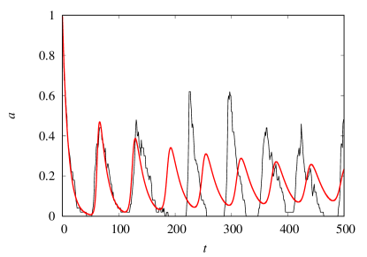
Figure 1: Time evolution of the fraction of active ants $a(t)$ for a population of size $N=50$ and rest period $\tau=49$. The jagged thin curve is the result of a single run of the Monte Carlo simulation and the smooth thick curve is the numerical solution of the mean-field equations. The other parameters are $\mu=1/10$, $\alpha=1/500$ and $\beta=1$. The initial conditions are $a(t)=0$ for $t\in[-\tau,0)$, $a(0)=1$, $b(0)=0$ and $s(0)=0$.

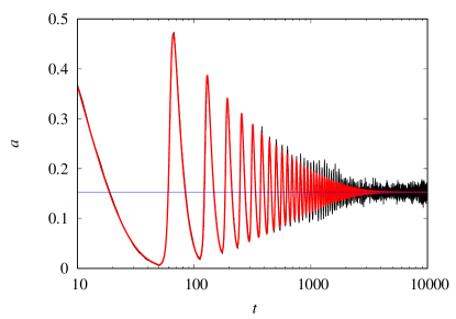
Figure 2: Time evolution of the fraction of active ants $a(t)$ for a population of size $N=5000$ and rest period $\tau=49$. The jagged thin curve is the result of a single run of the Monte Carlo simulation and the smooth thick curve is the numerical solution of the mean-field equations. The other parameters are $\mu=1/10$, $\alpha=1/500$ and $\beta=1$. The fixed point is $a^{*}\approx 0.153$ (thin horizontal line), $b^{*}\approx 0.099$ and $s^{*}\approx 0.748$. The initial conditions are $a(t)=0$ for $t\in[-\tau,0)$, $a(0)=1$, $b(0)=0$ and $s(0)=0$.

IV Fixed point analysis

The fixed point or equilibrium solutions $a^{*}=a(t)$, $b^{*}=b(t)$ and $s^{*}=s(t)$ are obtained by setting the time derivatives to zero in the mean-field equations (7), (8) and (9). The difficulty here is that this procedure yields only one equation, viz.,

$$b^{*}=\frac{\mu a^{*}}{\alpha+\beta a^{*}},$$ (10)

and so we need one more equation to determine the equilibrium solution unambiguously, since $a^{*}+b^{*}+s^{*}=1$. The missing equation is found by integrating Eq. (9) from $0$ to $n\tau$ where $n$ is an integer,

$$\int_{0}^{n\tau}\frac{ds}{dt}dt=\mu\left[\int_{0}^{n\tau}a(t)dt-\int_{0}^{n\tau}a(t-\tau)dt\right],$$ (11)

which, after some elementary manipulations, can be rewritten as

$$s(n\tau)-s(0)=\mu\left[\int_{n\tau-\tau}^{n\tau}a(t)dt-\int_{-\tau}^{0}a(t)dt\right].$$ (12)

Now, taking the limit $n\to\infty$ and assuming that the dynamics reach the equilibrium solution, we get

$$s^{*}-s(0)=\mu\left[\tau a^{*}-\int_{-\tau}^{0}a(t)dt\right].$$ (13)

We recall that for $t\in[-\tau,0)$ the fraction of active ants $a(t)$ is given by the initial conditions, which in turn determines the fraction of inactive ants at $t=0$, viz., $s(0)=\mu\int_{-\tau}^{0}a(t)dt$. Therefore,

$$s^{*}=\mu\tau a^{*}$$ (14)

regardless of the initial conditions. Using equations (10) and (14) together with the normalization condition gives the equation for the fraction of active ants at equilibrium,

$$\beta(1+\mu\tau)(a^{*})^{2}+\left[\alpha(1+\mu\tau)+\mu-\beta\right]a^{*}-\alpha=0.$$ (15)

This quadratic equation always has real roots: one negative and the other positive less than $1$, so the fixed points are physical (i.e., $a^{*}$, $b^{*}$ and $s^{*}$ are positive and less than $1$) for all parameter settings. As a good approximation, we can write $a^{*}\approx 1/\mu\tau$, $b^{*}\approx 1/\alpha\tau$ and $s^{*}\approx 1-(\mu+\alpha)/\mu\alpha\tau$, which holds for $\mu\tau\gg 1$.

To study the stability of the fixed point solutions Murray_2007 , we must first linearize equations (7) and (9) about the equilibrium $a^{*}$ and $s^{*}$ by writing

$$a(t) = a^{*}+\epsilon_{a}(t)$$ (16)

$$s(t) = s^{*}+\epsilon_{s}(t),$$ (17)

where the small perturbations $\epsilon_{a}$ and $\epsilon_{s}$ obey the linear equations

$$\frac{d\epsilon_{a}}{dt} = \left(-\mu+\beta-\alpha-2\beta a^{*}-\beta s^{*}\right)\epsilon_{a}(t)-\left(\alpha+\beta a^{*}\right)\epsilon_{s}(t)$$

$$\frac{d\epsilon_{s}}{dt} = \mu\left[\epsilon_{a}(t)-\epsilon_{a}(t-\tau)\right].$$ (19)

The next step is to look for solutions of the form $\epsilon_{a}(t)=\epsilon_{a}(0)e^{\lambda t}$ and $\epsilon_{s}(t)=\epsilon_{s}(0)e^{\lambda t}$, where $\epsilon_{a}(0)\ll 1$ and $\epsilon_{s}(0)\ll 1$ are constants. These solutions exist if the eigenvalues $\lambda$ satisfy the transcendental equation

$$\lambda\left(\lambda+X\right)+\left(1-e^{-\lambda\tau}\right)Y=0,$$ (20)

where $X=\mu-\beta+\alpha+\beta a^{*}(2+\mu\tau)$ and $Y=\mu(\alpha+\beta a^{*})$ are auxiliary variables. Setting $\lambda=u+iv$ we get the following equations for the real and imaginary parts of $\lambda$,

$$u^{2}-v^{2}+uX+Y = Ye^{-u\tau}\cos(v\tau)$$ (21)

$$-v(2u+X) = Ye^{-u\tau}\sin(v\tau).$$ (22)

It is clear from these equations that if $v$ is a solution, then so is $-v$, so we can consider $v>0$ without loss of generality. Note that $u=v=0$ (i.e., $\lambda=0$) is a solution. There is another solution with $u=0$ but $v>0$ which will prove to be important in determining the stability of the fixed point solutions as well as the period of the small amplitude oscillations. By squaring and summing these equations, we can write $v$ in terms of $u$ by solving the quadratic equation

$$w^{2}+w\left[2u(u+X)+X^{2}-2Y\right]$$

$$+\left[u(u+X)+Y\right]^{2}-Y^{2}e^{-2u\tau} = 0$$ (23)

with $w=w(u)=v^{2}$. So $u$ is given by the roots of $f(x)$, where

$$f(x)=(2x+X)\sqrt{w}+Ye^{-x\tau}\sin(\tau\sqrt{w})$$ (24)

and $w=w(x)$ are the solutions of Eq. (IV) with $u$ replaced by $x$. Recall that the fixed point solution is unstable if $u=\mbox{Re}(\lambda)>0$.

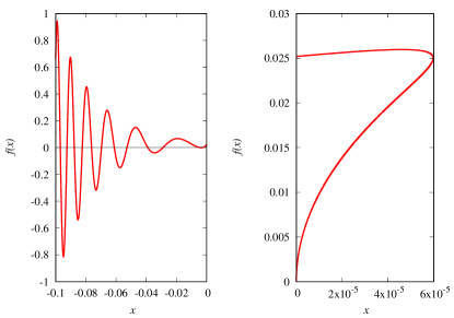
Figure 3: Function $f(x)$ whose roots are the real part of the eigenvalue $\lambda$ for the rest period $\tau=40$. There are infinitely many negative roots (left panel) but no positive roots (right panel) so the fixed point $a^{*}\approx 0.180$, $b^{*}\approx 0.099$, $s^{*}\approx 0.721$ is stable. The parameters are $\mu=1/10$, $\alpha=1/500$ and $\beta=1$.

Figure 3 shows the function $f(x)$ defined in Eq, (24) for $\tau=40$. There are infinitely many negative roots, but no positive roots, so the fixed point is stable. For $x<0$, the quadratic equation (IV) has only one positive solution. The other solution is negative and therefore not physical. For $x>0$, the two solutions of equation (IV) are positive, so $f(x)$ has two branches. For large $x>0$, the quadratic equation (IV) has no real roots. From now on we will focus only on the region $x\geq 0$, since a positive root of $f(x)$ would imply the instability of the fixed point.

Figure 4 shows $f(x)$ for several values of the rest period $\tau$. The results show that a positive root first appears when $x=0$ is a double root of $f(x)$, i.e. when the two branches of $f(x)$ coincide at $x=0$. More specifically, if we set $x=0$ in equation (IV) we get that the first branch is determined by the solution $w=0$, which gives $f(0)=0$, and the second branch is determined by $w=2Y-X^{2}$, which gives $f(0)=g(\tau)$, where

$$g(\tau)=X\sqrt{2Y-X^{2}}+Y\sin(\tau\sqrt{2Y-X^{2}}).$$ (25)

Imposing $g(\tau)=0$ gives an equation for the value of $\tau=\tau_{c}$ at which the fixed point solution becomes unstable. This is still quite a formidable equation, since the auxiliary variables $X=X(\tau)$ and $Y=Y(\tau)$ have a complicated dependence on $\tau$ through the fixed point $a^{*}$. Next, we show how to solve it numerically.

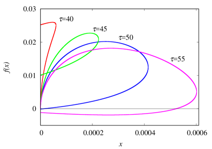
Figure 4: Function $f(x)$ whose roots are the real part of the eigenvalue $\lambda$ for rest period $\tau=40$, $45$, $50$ and $55$ as indicated. The parameters are $\mu=1/10$, $\alpha=1/500$ and $\beta=1$.

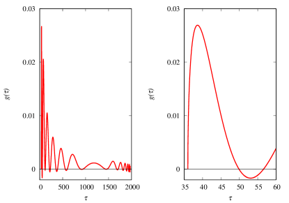
Figure 5: Function $g(\tau)$ whose smallest root within the open interval $(\tau_{l},\tau_{u})$ gives the critical rest period $\tau_{c}$ for $\mu=1/10$, $\alpha=1/500$ and $\beta=1$. The left panel shows $g(\tau)$ in the entire domain $\tau\in\left[35.98,1972.20\right]$ and the right panel zooms in on the region around the root $\tau_{c}\approx 49.902$.

Figure 5 shows the function $g(\tau)$ for the same values of the parameters $\alpha$ and $\mu$ used so far. We recall that $g(\tau)$ gives the values of $f(0)$ obtained with the solution $v^{2}=w=2Y-X^{2}$ shown in Fig. 4. Thus the domain of $g(\tau)$ is determined by the values of $\tau$ for which $w\geq 0$. We find numerically that, for the parameters used in this figure, this condition is satisfied in the interval $\tau\in\left[\tau_{l},\tau_{u}\right]$ where $\tau_{l}\approx 35.98$ and $\tau_{u}\approx 1972.20$. Note that $g(\tau_{l})=g(\tau_{u})=0$, but the root $\tau=\tau_{l}$ does not give $\tau_{c}$ because $\lim_{x\to 0^{+}}f(x)>0$ for $\tau\approx\tau_{l}$, as shown in Fig. 4 and in the right panel of Fig. 5. In words, $f(x)$ does not become negative when $\tau$ deviates from $\tau_{l}$. In fact, these figures show that $\tau_{c}$ is given by the smallest root of $g(\tau)$ within the open interval $\left(\tau_{l},\tau_{u}\right)$. In particular, we find $\tau_{c}\approx 49.902$ (or $\mu\tau_{c}\approx 4.99$). Thus, the rest period $\tau=50$ used in the original simulations of the autocatalytic ant colony model Goss_1988 gives truly periodic solutions in the limit of infinitely large populations, but because of its proximity to $\tau_{c}$ the amplitude of the oscillations is too small to be observed numerically.

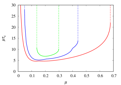
Figure 6: Scaled critical rest period above which the fixed point solutions are unstable as function of the inactivation probability $\mu$ for (bottom to top) $\alpha=1/500$, $1/50$ and $1/20$. As usual, $\beta=1$. The dashed vertical lines indicate the lower $\mu_{l}$ and upper $\mu_{u}$ bounds of the region of existence of period solutions for a given $\alpha$. For $\alpha=1/500$ we have $\mu_{l}\approx 0.0047$. Note the discontinuities in the derivative of $\tau_{c}$ at some singular points.

Figure 6 shows how the critical rest period $\tau_{c}$ is affected by the parameters $\mu$ and $\alpha$, which we previously held fixed. The results show the complexity of the problem. It turns out that the regime of periodic solutions exists only in a limited region of the parameter space. For a fixed $\alpha$, there is an upper bound $\mu_{u}$ on the inactivation probability beyond which the fixed-point solution is stable, regardless of how large the rest period $\tau$ is. Note that $\tau_{c}$ does not diverge at $\mu=\mu_{u}$: the transition line simply ends at this upper bound because $g(\tau)$ has no roots except the domain extremes $\tau_{l}$ and $\tau_{u}$. The same happens for the lower bound $\mu_{l}$, below which the fixed point solution is stable. Most interestingly, increasing $\alpha$ decreases the range of parameters where the periodic solutions exist, until these solutions disappear altogether at $\alpha=\alpha_{c}$. In other words, for $\alpha>\alpha_{c}\approx 0.0589$ the fixed point solutions are stable regardless of the values of $\mu$ and $\tau$.

In order to understand the results summarized in Fig. 6, let us look at the case $\alpha=1/20$ in more detail. Figure 7 shows what happens for $\mu$ in the vicinity of $\mu_{l}$ and $\mu_{u}$ and indicates how these parameters can be calculated by finding the double root of $g(\tau)$. In fact, near these extremes, this pattern of variation of $g(\tau$) occurs for all values of $\alpha$, so we can use the criterion that $g(\tau)$ becomes negative, leading to the appearance of an eigenvalue with a positive real part, by a double root to determine the region in parameter space where the periodic solutions exist. In practice, this criterion boils down to determining whether the minimum of $g(\tau)$ is positive or negative. We just note that for small $\alpha$, the pattern shown in Fig. 7 appears only very close to $\mu_{l}$.

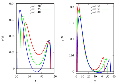
Figure 7: Function $g(\tau)$ whose smallest root within the open interval $(\tau_{l},\tau_{u})$ gives the critical rest period $\tau_{c}$ for $\alpha=1/20$ and $\beta=1$. The left panel shows the results for (top to bottom at $\tau=70$) $\mu=0.13$, $0.135$ and $0.14$. The double root occurs at $\mu=\mu_{l}\approx 0.1374$ and $\tau_{c}\approx 79.43$. The right panel shows the results for (top to bottom at $\tau=40$) $\mu=0.32$, $0.30$ and $0.28$. The double root occurs at $\mu=\mu_{u}\approx 0.298$ and $\tau_{c}\approx 33.62$.

Figure 8 shows the region in the parameter space $(\mu,\alpha)$ where the fixed-point solutions are unstable for some choices of the rest period $\tau$. Outside this region, the fixed-point solutions are stable, regardless of the value of $\tau$. The key parameter here is the spontaneous activation probability $\alpha$, which acts as a noise that disturbs the synchrony resulting from the autocatalytic activation of the ants by contact between active and activatable inactive ants. As already pointed out, the maximum amount of noise compatible with synchronization is $\alpha=\alpha_{c}\approx 0.0589$, obtained for $\mu\approx 0.21$. Interestingly, this disruptive effect of spontaneous activation is enhanced by either increasing or decreasing the probability of inactivation $\mu$, as already shown in Fig. 6. Of course, for large $\mu$, an active ant is likely to become inactive before it finds an activatable inactive ant, reducing the effectiveness of the autocatalytic activation synchronization mechanism. For small $\mu$, there are so many active ants at any time that the synchronizing effect of the rest period $\tau$ becomes ineffective: whenever an ant wakes up, it is activated.

Figure 8: Values of the inactivation probability $\mu$ and the spontaneous activation probability $\alpha$ (shaded region) for which the fixed-point solutions are unstable for some values of the rest period $\tau$ and the delay differential equations exhibit periodic solutions. As usual, $\beta=1$.

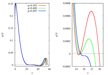
Figure 9: Function $g(\tau)$ whose smallest root within the open interval $(\tau_{l},\tau_{u})$ gives the critical rest period $\tau_{c}$ for $\alpha=1/50$ and $\beta=1$. The left panel shows the results in the entire domain for $\mu=0.395$, $0.400$ and $0.405$ and the right panel zooms in on the vicinity of $\tau_{c}$.

Another curious feature shown in Fig. 6 is the existence of singular points where the derivatives of $\tau_{c}$ with respect to $\mu$ are discontinuous. The scale of the figure obscures this phenomenon somewhat, but it will become more conspicuous when we consider the periodic solutions near $\tau_{c}$. The singularity is due to a change in the character of the smallest root of $g(\tau)$ as shown in Fig. 9 for $\alpha=1/50$. What happens is that for some value of $\mu\in\left(0.4,0.405\right)$, $\tau_{c}$ is given by a triple root, and merging the three smallest roots (excluding the lower extreme $\tau_{l}$) of $g(\tau)$ yields a root that behaves differently than the smallest root before the merge. The point here is that these singularities are not artifacts of the numerical procedure used to find the roots of $g(\tau)$, but, unlike the phenomenon that gives rise to $\mu_{l}$ and $\mu_{u}$, they have no implications on the nature of the asymptotic solutions of the mean-field equations.

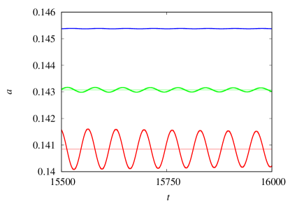
Figure 10: Fraction of active ants $a(t)$ for rest period (top to bottom) $\tau=52,53$ and $54$. The other parameters are $\mu=1/10$, $\alpha=1/500$ and $\beta=1$. The fixed point solutions are stable for $\tau<49.902$. The thin horizontal lines indicate the unstable fixed point $a^{*}$, given by Eq. (15). The initial conditions are $a(t)=0$ for $t\in[-\tau,0)$, $a(0)=1$, $b(0)=0$ and $s(0)=0$.

V Periodic solutions

The first important result about the periodic solutions of the system of delay differential equations (7)-(9) is that the period $T$ must be different from $\tau$, otherwise $s(t)$ would not be periodic. The second is that the amplitude of the oscillations becomes arbitrarily small as $\tau$ approaches $\tau_{c}$ for $\mu$ and $\alpha$ fixed, as shown in Fig. 10 for $\mu=1/10$ and $\alpha=1/500$. The oscillations for $\tau=52$ are barely noticeable on the already narrow scale of the figure, which is why we claim that the oscillations observed in the original simulations of the model for $\tau=50$ are a finite-size artifact Goss_1988 . However, this result allows to estimate the period $T$ for $\tau\approx\tau_{c}$, where the model is described by the linear equations (IV) and (19). In fact, in this case the period is simply $T=2\pi/v$ where $v>0$ is the imaginary part of the eigenvalue $\lambda$ when its real part $u$ vanishes. We recall that the condition $u=0$, which implies $v=\sqrt{2Y-X^{2}}$, determines the critical rest period $\tau_{c}$, as shown in Fig. 4.

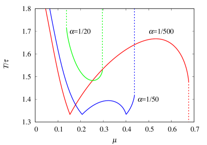
Figure 11: Ratio between the period $T$ of the periodic solutions and the rest period at $\tau=\tau_{c}$ for $\alpha=1/500$, $1/50$ and $1/20$ as indicated. As usual, $\beta=1$. The dashed vertical lines indicate the lower $\mu_{l}$ and upper $\mu_{u}$ bounds of the region of existence of period solutions for a given $\alpha$.

Figure 11 shows the ratio $T/\tau$ for the periodic solutions near $\tau=\tau_{c}$. Recall that the periodic solutions exist only in the interval $\left[\mu_{l},\mu_{u}\right]$. Note that both $T$ and $\tau_{c}$ vary with $\mu$ and $\alpha$, which explains the complexity of the results (the plot of $\mu T$ versus $\mu$ is very similar to Fig. 6), but the rest period is clearly the natural scale for measuring the period of the oscillations. In particular, we find $T>\tau$, as expected. In fact, an ant should go through three stages in a cycle: inactive, which takes exactly a time $\tau$, activatable inactive, which takes time $1/(\alpha+\beta a^{*})$ on average, and active, which takes time $1/\mu$ on average. So the period $T$ must be greater than the the rest period $\tau$. The singularities that were barely noticeable in Fig. 6 are now very prominent, but they do not seem to have any physically relevant implications.

VI Discussion

The autocatalytic ant colony model generates periodic synchronized rhythms thanks to the synergy between two key components, viz. the activation of activatable inactive ants by active ants, whose strength is determined by the parameter $\beta$, and the rest period $\tau$ of inactive ants. None of these components alone can produce periodic solutions to the mean-field equations (7)-(9) describing an ant colony of infinite size. In fact, on the one hand, Fig. 6 shows that there is a minimum value of the rest period $\tau_{c}>0$ above which the periodic solutions appear, so that a sufficiently large rest period is a necessary condition for observing periodic synchronized rhythms in the model. On the other hand, Fig. 8 shows that for small values of $\beta$, which correspond to large values of $\alpha$, there are no periodic solutions to the mean-field equations, regardless of the value of the rest period $\tau$. As a matter of fact, this figure shows that the range of parameters for which the periodic solutions exist is very limited. We note that in the original simulations of the model using a colony of size $N=50$, unsynchronized activity was reported when the rest period $\tau$ was too short relative to the activity period ($1/\mu$) or when the activation coefficient $\beta$ was too low Goss_1988 .

We emphasize that our only analytical evidence for considering the periodic solutions as stable limit cycles, i.e., when perturbed, the solution returns to the original periodic solution in the limit $t\to\infty$ and the periodic behavior is independent of the initial conditions, is the instability of the fixed-point solutions (the real part of the eigenvalues $\lambda$ given by Eq. (20) are positive). This contrasts with the periodic solutions of conservative systems, for which the real part of the eigenvalues of the community matrix are zero and the phase space trajectories are closed orbits depending on the initial conditions Murray_2007 . Since this evidence is certainly not conclusive, we complemented it with an extensive numerical study of the mean-field equations, which showed that when the fixed-point solutions are unstable, the periodic solutions are indeed the only attractors of the dynamics.

The neatness of the autocatalytic ant colony model Goss_1988 makes it easy to implement through Monte Carlo simulations, but the results are not easy to interpret without knowledge of the nature of the equilibrium solutions. Our main contribution is the derivation of mean-field delay differential equations, which are exact in the limit $N\to\infty$, but give a good fit to the simulation results already for colony sizes on the order of a few thousand ants, as shown in Fig. 2. A standard, but rather complicated, analysis of the equilibrium solutions of these equations indicates that both the unsynchronized and synchronized activity patterns observed in the short-time simulations for small $N$ are fluctuations due to finite-size effects. In fact, these fluctuations make it virtually impossible to distinguish true periodic solutions from damped oscillations that eventually settle to a fixed point, as shown in Figs. 1 and 2. In particular, the reported unsynchronized activity patterns Goss_1988 are fluctuations around stable fixed points. Note, however, that the colony sizes used in the laboratory experiments range from $7$ to $250$ ants, so the small $N$ simulations are probably more realistic than our mean-field formulation. The large finite-size fluctuations make it very difficult to elucidate the role of the model parameters and, in particular, to appreciate the various threshold phenomena associated with the instability of the fixed-point solutions.

Finally, we note that there is no consensus biological explanation for the existence of short-term activity cycles in colonies of some ant species. Although there are suggestions that these cycles promote more efficient brood care Goss_1988 , another explanation is that they are inevitable results of interactions between ants, without any adaptive significance, i.e., they are epiphenomena Cole_1991 . However, our analysis shows that the periodic solutions are far from inevitable and exist only in a small region of the parameter space. Of course, these parameters may be subject to selective pressures, an issue that can be addressed using a group selection approach, similar to what has been done to evolve response thresholds Bonabeau_1998 in the context of division of labor Duarte_2012 ; Fontanari_2023 . Indeed, this seems to be a natural context for considering the activity cycles of ant colonies, where there is only a distinction between inactivity and movement activity, which is a prerequisite for other types of behavior Cole_1991 .

References

References

- (1) G. Nicolis, I. Prigogine, Self-Organization in Nonequilibrium Systems: From Dissipative Structures to Order Through Fluctuations, Wiley, New York, 1977.
- (2) R.M. May, Stability and Complexity in Model Ecosystems, Princeton University Press, Princeton, 1975.
- (3) D.J.T. Sumpter, Collective Animal Behavior, Princeton University Press, Princeton, 2010.
- (4) S.H. Strogatz, I. Stewart, Coupled oscillators and biological synchronization, Sci. Amer. 269 (1993) 102–109.
- (5) S.H. Strogatz, From Kuramoto to Crawford: exploring the onset of synchronization in populations of coupled oscillators, Phys. Nonlinear Phenom. 143 (2000) 1–20.
- (6) N.R. Franks, S. Bryant, R.Griffiths, L. Hemerik, Synchronization of the behaviour within nests of the ant Leptothorax acervorum (Fabricuis) –I. Discoveringt he phenomenon and its relation to the level of starvation, Bull. Math. Biol. 52 (1990) 597–612.
- (7) B.J. Cole, Short-Term Activity Cycles in Ants: Generation of Periodicity by Worker Interaction, Am. Nat. 137 (1991) 244–259.
- (8) G.N. Doering, B. Drawert, C. Lee, J.N. Pruitt, L.R. Petzold, K. Dalnoki-Veress, Noise resistant synchronization and collective rhythm switching in a model of animal group locomotion, R. Soc. Open Sci. 9 (2022) 211908.
- (9) L. Hemerik, N.R. Franks, N. Britton, Synchronization of the behaviour within nests of the ant Leptothorax acervorum (Fabricius) – II. Modelling the phenomenon and predictions from the model, Bull. Math. Biol. 52 (1990) 613–628.
- (10) S. Goss, J.L. Deneubourg, Autocatalysis as a source of synchronised rhythmical activity in social insects, Insectes Soc. 35 (1988) 310–315.
- (11) C. Tofts, M. Hatcher, N.R. Franks, The Autosynchronization of the Ant Leptothorax acervorum (Fabricius): Theory, Testability and Experiment, J. Theor. Biol. 157 (1992) 71–82.
- (12) K. Huang, Statistical Mechanics, John Willey & Sons, New York, 1963.
- (13) W. Feller, An Introduction to Probability Theory and Its Applications, Vol. 1, Third Edition, Wiley, New York, 1968.
- (14) J.D. Murray, Mathematical Biology: I. An Introduction, Springer, New York, 2007, pp. 17–21.
- (15) E. Bonabeau, G. Theraulaz, J.L. Deneubourg, Fixed response thresholds and the regulation of division of labor in insect societies, Bull. Math. Biol. 60 (1998) 753–807.
- (16) A. Duarte, I. Pen, L. Keller, F.J. Weissing, Evolution of self-organized division of labor in a response threshold model, Behav. Ecol. Sociobiol. 66 (2012) 947–957.
- (17) J.F. Fontanari, V.M. Oliveira, P.R.A. Campos, Evolving division of labor in a response threshold model, https://doi.org/10.48550/arXiv.2308.07122